STA 260: Statistics and Probability II - University of Torontonosedal/sta260/sta260-chap6.pdf · The Method of Distribution Functions The Method of Transformations The Method of Moment-Generating

Chapter 6. Function of Random Variables

STA 260: Statistics and Probability II

Al Nosedal.University of Toronto.

Winter 2018

Al Nosedal. University of Toronto. STA 260: Statistics and Probability II


1 Chapter 6. Function of Random VariablesThe Method of Distribution FunctionsThe Method of TransformationsThe Method of Moment-Generating FunctionsOrder StatisticsBivariate Transformation MethodAppendix



”If you can’t explain it simply, you don’t understand it wellenough”

Albert Einstein.



The Method of Distribution FunctionsThe Method of TransformationsThe Method of Moment-Generating FunctionsOrder StatisticsBivariate Transformation MethodAppendix

Example

Let (Y1,Y2) denote a random sample of size n = 2 from theuniform distribution on the interval (0, 1). Find the probabilitydensity function for U = Y1 + Y2.




Solution

The density function for each Yi is

f (y) =

{1 0 ≤ y ≤ 10 elsewhere

Therefore, because we have a random sample, Y1 and Y2 areindependent, and

f (y1, y2) = f (y1)f (y2)

{1 0 ≤ y1 ≤ 1, 0 ≤ y2 ≤ 10 elsewhere

We wish to find FU(u) = P(U ≤ u).




Joint pdf

0.0 0.2 0.4 0.6 0.8 1.0

0.0

0.2

0.4

0.6

0.8

1.0

0.0

0.2

0.4

0.6

0.8

1.0

y1

y2f(y1,

y2)

●●

●●




Solution

The region y1 + y2 ≤ u for 0 ≤ u ≤ 1.

●●●●●●●●●●●●●●●●●●●●●●●●●●●●●●●●●●●●●●●●●●●●●●●●●●●●●●●●●●●●●●●●●●●●●●●●●●●●●●●●●●●●●●●●●●●●●●●●●●●●●

0.0 0.2 0.4 0.6 0.8 1.0

0.0

0.2

0.4

0.6

0.8

1.0

y1

y2

●

y1 + y2 < 1




Solution

The solution, FU(u), 0 ≤ u ≤ 1, could be acquired directly by usingelementary geometry.FU(u) = (area of triangle)(height) = u2

2 (1) = u2

2 .




Solution

The region y1 + y2 ≤ u for 1 < u ≤ 2.

●●●●●●●●●●●●●●●●●●●●●●●●●●●●●●●●●●●●●●●●●●●●●●●●●●●●●●●●●●●●●●●●●●●●●●●●●●●●●●●●●●●●●●●●●●●●●●●●●●●●●

0.0 0.2 0.4 0.6 0.8 1.0

0.0

0.2

0.4

0.6

0.8

1.0

y1

y2

●

●

●

●

y2 < u − y1




Solution

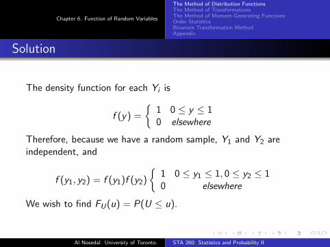
The solution, FU(u), 1 < u ≤ 2, could be acquired directly by usingelementary geometry, or using Calculus.

FU(u) = 1− (area of triangle)(height)

= 1−[

(2− u)(2− u)

2

](1)

= 1−[

2− 2u +u2

2

]= −1 + 2u − u2

2




Solution

It should be clear at this point thatIf u < 0, FU(u) = 0.If u > 2 FU(u) = 1.




Solution

To summarize,

FU(u) =

0 u ≤ 0u2/2 0 < u ≤ 1(−u2/2) + 2u − 1 1 < u ≤ 21 u > 2




Solution

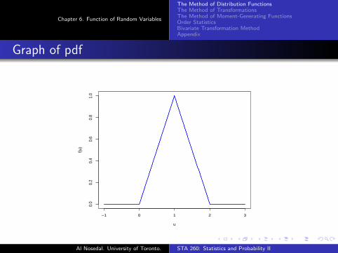
The density function fU(u) can be obtained by differentiatingFU(u). Thus,

fU(u) =d FU(u)

du=

0 u ≤ 0u 0 ≤ u ≤ 12− u 1 < u ≤ 20 u > 2




Graph of pdf

−1 0 1 2 3

0.0

0.2

0.4

0.6

0.8

1.0

u

f(u)




Example

Consider the case U = h(Y ) = Y 2, where Y is a continuousrandom variable with distribution function FY (y) and densityfunction fY (y). Find the probability density function for U.




Solution

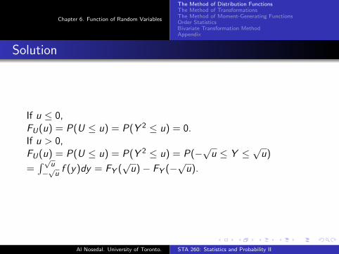
If u ≤ 0,FU(u) = P(U ≤ u) = P(Y 2 ≤ u) = 0.If u > 0,FU(u) = P(U ≤ u) = P(Y 2 ≤ u) = P(−

√u ≤ Y ≤

√u)

=∫ √u−√uf (y)dy = FY (

√u)− FY (−

√u).




Solution

On differentiating with respect to u, we see that

fU(u) =

{1

2√u

[fY (√u) + fY (−

√u)] u > 0

0 otherwise




Exercise 6.7

Suppose that Z has a standard Normal distribution.a. Find the density function of U = Z 2.b. Does U have a gamma distribution? What are the values of αand β?c. What is another name for the distribution of U?




Solution

Let FZ (z) and fZ (z) denote the standard Normal distribution anddensity functions respectively.a. FU(u) = P(U ≤ u) = P(Z 2 ≤ u) = P(−

√u ≤ Z ≤

√u)

= FZ (√u)− FZ (−

√u).

The density function for U is thenfU(u) = F

′U(u) = 1

2√ufZ (√u) + 1

2√ufZ (−

√u), u ≥ 0.




Solution

Recalling that fZ (z) = 1√2πe−

z2

2 , we find

fU(u) = 12√u

1√2πe−

u2 + 1

2√u

1√2πe−

u2

fU(u) = 1√π√

2u−1/2e−u/2, u > 0.




Solution

b. U has a gamma distribution with α = 1/2 and β = 2 (recallthat Γ(1/2) =

√π).

c. This is the chi-square distribution with one degree of freedom.




Weibull density function

The Weibull density function is given by

f (y) =

{1αmym−1e−y

m/α y > 0,0, elsewhere,

where α and m are positive constants. This density function isoften used as a model for the lengths of life of physical systems.




Exercise 6.27

Let Y have an exponential distribution with mean β. Prove thatW =

√Y has a Weibull density with α = β and m = 2.




Solution

Let W =√Y . The random variable Y is exponential so

fY (y) = 1β e−y/β.

Step 1. Then, Y = W 2.Step 2. dy

dw = 2w .Step 3. Then,

fW (w) = fY (w2)|2w | =(

1β e−w2/β

)(2w) = 2

βwe−w2/β, w ≥ 0,

which is Weibull with m = 2.




Exercise 6.28

Let Y have a uniform (0, 1) distribution. Show that W = −2ln(Y )has an exponential distribution with mean 2.




Solution

Step 1. Then, Y = e−w/2.Step 2. dy

dw = −12 e−w/2.

Step 3. Then, fW (w) = fY (e−w/2)|−12 e−w/2| = 1

2e−w/2,w > 0.




Exercise 6.29 a.

The speed of a molecule in a uniform gas at equilibrium is arandom variable V whose density function is given byf (v) = av2e−bv

2, v > 0, where b = m/2kT and k ,T , and m

denote Boltzmann’s constant, the absolute temperature, and themass of the molecule, respectively.Derive the distribution of W = mV 2/2, the kinetic energy of themolecule.




Solution

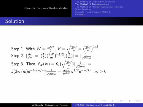
Step 1. With W = mV 2

2 , V =√

2Wm =

(2Wm

)1/2.

Step 2. | dvdw | = |( 12 )( 2W

m )−1/2)( 2m )| = | 1√

2mw|.

Step 3. Then, fW (w) = fV (√

2Wm )| 1√

2mw| =

a(2w/m)e−b(2w/m) 1√2mw

= a√

2m3/2w

1/2e−w/kT , w > 0.




Solution

The above expression looks like a Gamma density with α = 3/2and β = kT . Thus, the constant a must be chosen so that

a√

2

m3/2=

1

Γ(3/2)(KT )3/2.

So,

fW (w) =1

Γ(3/2)(KT )3/2w1/2e−w/kT .




Example

Let Z be a Normally distributed random variable with mean 0 andvariance 1. Use the method of moment-generating functions tofind the probability distribution of Z 2.




Solution

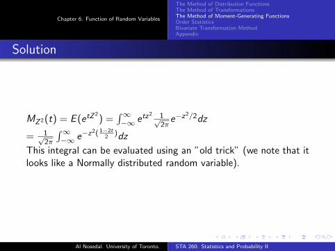
MZ2(t) = E (etZ2) =

∫∞−∞ etz

2 1√2πe−z

2/2dz

= 1√2π

∫∞−∞ e−z

2( 1−2t2

)dz

This integral can be evaluated using an ”old trick” (we note that itlooks like a Normally distributed random variable).




Solution

We realize that e−z2( (1−2t)

2) is proportional to a Normal with µ = 0

and σ2 = 1/(1− 2t), then

MZ2(t) =√

2π√

1/(1−2t)√2π

∫∞−∞

1√2π√

1/(1−2t)e−z

2( 1−2t2

)dz

MZ2(t) =√

11−2t = (1− 2t)−1/2 (Note. This is valid provided

that t < 1/2).(1− 2t)−1/2 is the moment-generating function for agamma-distributed random variable with α = 1/2 and β = 2.Hence, Z 2 has a χ2 distribution with ν = 1 degree of freedom.




Exercise 6.40

Suppose that Y1 and Y2 are independent, standard Normal randomvariables. Find the probability distribution of U = Y 2

1 + Y 22 .




Solution

MU(t) = E [eUt ] = E [e(Y 21 +Y 2

2 )t ]

= E [eY21 teY

22 t ] (by independence)

= E [eY21 t ]E [eY

22 t ]

= MY 21

(t)MY 22

(t)

= [(1− 2t)−1/2][(1− 2t)−1/2] = (1− 2t)−2/2.

Because moment-generating functions are unique, U has a χ2

distribution with 2 degrees of freedom.




Comment about last example

Note that (1− 2t)−2/2 = (1− 2t)−1 which is themoment-generating function of an exponential random variablewith parameter β = 2. Which is the right probability distribution?χ2 with 2 df? Exponential with β = 2? Let us write the pdf foreach of them.Exponential pdf with β = 2.f (y) = 1

2e−y/2, 0 < y <∞.

Chi-square pdf with ν = 2.

f (y) = y2/2−1

22/2Γ(2/2)e−y/2 = 1

2e−y/2, 0 < y <∞.

They are the same!




Example

Let Y1 and Y2 be independent, Normal random variables, eachwith mean µ and variance σ2. Let a1 and a2 denote knownconstants. Find the density function of the linear combinationU = a1Y1 + a2Y2.




Solution

The mgf for a Normal distribution with parameters µ and σ ism(t) = eµt+σ2t2/2.

MU(t) = E [eUt ] = E [e(a1Y1+a2Y2)t ]

= E [e(a1Y1)te(a2Y2)t ] (by independence)

= E [e(a1Y1)t ]E [e(a2Y2)t ]

= MY1(a1t)MY2(a2t)

= [eµa1t+σ2(a1t)2/2][eµa2t+σ2(a2t)2/2]

= eµt(a1+a2)+σ2(a21+a2

2)t2/2

This is the mgf for a Normal variable with mean µ(a1 + a2) andvariance σ2(a2

1 + a22).




Example

Let Y1 and Y2 be independent, Normal random variables, each withmean µ and variance σ2. Find the density function of Y = Y1+Y2

2 .




Solution

From our previous example and making a1 = a2 = 12 , we have that

Y has a Normal distribution with mean µ and variance σ2/2.




Exercise 6.59

Show that if Y1 has a χ2 distribution with ν1 degrees of freedomand Y2 has a χ2 distribution with ν2 degrees of freedom, thenU = Y1 + Y2 has a χ2 distribution with ν1 + ν2 degrees offreedom, provided that Y1 and Y2 are independent.




Exercise 6.72 a.

Let Y1 and Y2 be independent and uniformly distributed over theinterval (0, 1). Find the probability density function ofU = min(Y1,Y2).




Solution

Let U = min(Y1,Y2).FU(u) = P(U ≤ u) = 1− P(U > u). Now, let us find P(U > u).P(U > u) = P(min(Y1,Y2) > u) = [P(Y1 > u)][P(Y2 > u)]P(U > u) = [1− P(Y1 ≤ u)][1− P(Y2 ≤ u)]P(U > u) = [1− u]2

Therefore, FU(u) = P(U ≤ u) = 1− [1− u]2.Finally, fU(u) = d

duFU(u) = −2(1− u)(−1) = 2(1− u), 0 < u < 1.




Exercise 6.73 a.

Let Y1 and Y2 be independent and uniformly distributed over theinterval (0, 1). Find the probability density function ofU2 = max(Y1,Y2).




Solution

Let U = max(Y1,Y2).FU(u) = P(U ≤ u) = P(max(Y1,Y2) ≤ u)= P(Y1 ≤ u)P(Y2 ≤ u) = (u)(u) = u2.Therefore, FU(u) = u2.Finally, fU(u) = d

duFU(u) = 2u, 0 < u < 1.




Example

Let Y1,Y2, ...,Yn be independent, uniformly distributed randomvariables on the interval [0, θ]. Find the pdf of Y(n).




Solution

Let U = max(Y1,Y2, ...,Yn).FU(u) = P(U ≤ u) = P(max(Y1,Y2, ...,Yn) ≤ u)= P(Y1 ≤ u)P(Y2 ≤ u)...P(Yn ≤ u) = (u/θ)(u/θ)...(u/θ).Therefore, FU(u) = (u/θ)n.

Finally, fU(u) = dduFU(u) = nun−1

θn , 0 ≤ u ≤ θ.




Example

The values x1 = 0.62, x2 = 0.98, x3 = 0.31, x4 = 0.81, andx5 = 0.53 are the n = 5 observed values of five independent trialsof an experiment with pdf f (x) = 2x , 0 < x < 1. The observedorder statistics arey1 = 0.31 < y2 = 0.53 < y3 = 0.62 < y4 = 0.81 < y5 = 0.98.Recall that the middle observation in the ordered arrangement,here y3 = 0.62 is called the sample median and the difference ofthe largest and the smallest herey5 − y1 = 0.98− 0.31 = 0.67,is called the sample range.




If X1,X2, ...,Xn are observations of a random sample of size n froma continuous-type distribution, we let the random variablesY1 < Y2 < ... < Yn

denote the order statistics of that sample. That is,Y1 = smallest of X1,X2, ...,Xn,Y2 = second smallest of X1,X2, ...,Xn,. . .

Yn = largest of X1,X2, ...,Xn.




Example

Let Y1 < Y2 < Y3 < Y4 < Y5 be the order statistics of a randomsample X1,X2,X3,X4,X5 of size n = 5 from the distribution withpdf f (x) = 2x , 0 < x < 1. Consider P(Y4 ≤ 1/2).




Example (cont.)

For the event Y4 ≤ 1/2 to occur, at least four of the randomvariables X1,X2,X3,X4,X5 must be less than 1/2.Thus if the event Xi ≤ 1/2, i = 1, 2, ..., 5, is called ”success” wemust have at least four successes in the five mutually independenttrials, each of which has probability of success

P(Xi ≤ 1

2

)=∫ 1/2

0 2xdx =(

12

)2= 1

4Thus,P(y4 ≤ 1

2

)=(5

4

) (14

)4 (34

)+(

14

)5= 0.0156




Example (cont.)

In general, if 0 < y < 1, then the distribution function of Y4 is

G (y) = P(Y4 ≤ y) =

(5

4

)(y2)4 (

1− y2)

+(y2)5

since this represents the probability of at least four ”successes” infive independent trials, each of which has probability of success

P(Xi ≤ y) =

∫ y

02xdx = y2.




Example (cont.)

The pdf of Y4 is therefore, for 0 < y < 1,

g(y) = G′(y) =

(5

4

)4(y2)3(2y)(1−y2)+

(5

4

)(y2)4(−2y)+5(y2)4(2y)

g(y) =5!

3!1!(y2)3(1− y2)(2y), 0 < y < 1.

Note that in this example, the cumulative distribution function ofeach X is FX (x) = x2 when 0 < x < 1. Thus

g(y) =5!

3!1![FX (y)]3(1− FX (y)]f (y), 0 < y < 1.




Theorem 6.5

Let Y1,Y2, ...,Yn be independent identically distributed continuousrandom variables with common distribution function F (y) andcommon density function f (y). If Y(k) denotes the kth-orderstatistic, then the density function of Y(k) is given by

g(k)(yk) =n!

(k − 1)!(n − k)[F (yk)]k−1[1− F (yk)]n−k f (yk),

∞ < yk <∞




Bivariate Transformation Method

Let X1 and X2 be jointly continuous random variables with jointprobability density function fX1, X2 . It is sometimes necessary toobtain the joint distribution of the random variables Y1 and Y2,which arise as functions of X1 and X2. Specifically, suppose thatY1 = g1(X1,X2) and Y2 = g2(X1,X2) for some functions g1 andg2. Assume that the functions g1 and g2 satisfy the followingconditions:1. The equations y1 = g1(x1, x2) and y2 = g2(x1, x2) can beuniquely solved for x1 and x2 in terms of y1 and y2 with solutionsgiven by, say, x1 = h1(y1, y2), x2 = h2(y1, y2).




Bivariate Transformation Method

2. The functions g1 and g2 have continuous partial derivatives atall points (x1, x2) and are such that the following 2× 2 determinant

J(x1, x2) = det

[∂g1∂x1

∂g1∂x2

∂g2∂x1

∂g2∂x2

]6= 0

at all points (x1, x2).Under these two conditions it can be shown that the randomvariables Y1 and Y2 are jointly continuous with joint densityfunction given byfY1, Y2(y1, y2) = fX1, X2(x1, x2)|J(x1, x2)|−1,where x1 = h1(y1, y2), x2 = h2(y1, y2) and |J(x1, x2)| is theabsolute value of the Jacobian.

(We will not prove this result, but it follows from Calculus resultsused for change of variables in multiple integration.)




Example

Let (X , Y ) denote a random point in the plane and assume thatthe rectangular coordinates X and Y are independent standardrandom Normal random variables. We are interested in the jointdistribution of R and Θ, the polar coordinate representation of thispoint (see Figure below).




Figure

0.0 0.5 1.0 1.5 2.0 2.5

0.0

0.5

1.0

1.5

2.0

2.5

X

YR

Θ

●




Example

Letting r = g1(x , y) =√x2 + y2 and θ = g2(x , y) = tan−1

( yx

),

we see that∂g1∂x = x√

x2+y2

∂g1∂y = y√

x2+y2

∂g2∂x = 1

1+(y/x)2

(− y

x2

)= −y

x2+y2

∂g2∂y = 1

x[1+(y/x)2]= x

x2+y2




Example

HenceJ = x2

(x2+y2)3/2 + y2

(x2+y2)3/2 = 1√x2+y2

= 1r .

As the joint density function of X and Y is

fX , Y (x , y) =1

2πe−(x2+y2)/2

we see that the joint density function of R =√

x2 + y2,Θ = tan−1(y/x), is given by

fR, Θ(r , θ) =1

2πre−r

2/2 0 < θ < 2π, 0 < r <∞.




Example

As this joint density factors into the marginal densities for R andΘ, we obtain that R and Θ are independent random variables, withΘ being uniformly distributed over (0, 2π) and R having theRayleigh distribution with density

fR(r) = re−r2/2 0 < r <∞.




Example

If we wanted the joint distribution of R2 and Θ, then, as thetransformation d = h1(x , y) = x2 + y2 andθ = h2(x , y) = tan−1(y/x) has a Jacobian

J = det

[2x 2y−y

x2+y2x

x2+y2

]= 2

we see that

fD, Θ(d , θ) =1

2e−d/2 1

2π0 < d <∞, 0 < θ < 2π.

Therefore, R2 and Θ are independent, with R2 having anexponential distribution with parameter β = 2.




We would like to show why Γ(1/2) =√π. First, we integrate a

standard Normal random variable over its entire domain.

1√2π

∫ ∞−∞

e−z2/2dz = 1

Notice that the integrand above is symmetric around 0. Thus,∫ ∞0

e−z2/2dz =

√2π

2=√π/2

Now, let w = z2

2 , which implies that dz = (2w)−1/2dw . Then∫ ∞0

e−z2/2dz =

∫ ∞0

(2w)−1/2e−wdw =√π/2




Our last equation is equivalent to∫ ∞0

(w)−1/2e−wdw =√π

Next, we multiply the last integral by a ”one”

Γ(1/2)

∫ ∞0

1

Γ(1/2)(w)−1/2e−wdw =

√π

We notice that the last integral equals one (we are integrating aGamma distribution over its entire domain). Therefore

Γ(1/2)(1) =√π




Homework?

Let X1 and X2 be jointly continuous random variables withprobability density function fX1,X2 . Let Y1 = X1 + X2,Y2 = X1 − X2. Find the joint density function of Y1 and Y2 interms of fX1,X2 .


Documents

STA 260: Statistics and Probability II - University of Torontonosedal/sta260/sta260-chap6.pdf · The Method of Distribution Functions The Method of Transformations The Method of Moment-Generating