Embed Size (px)
Citation preview

Session Number: Parallel Session 2A
Time: Monday, August 23, PM
Paper Prepared for the 31st General Conference of
The International Association for Research in Income and Wealth
St. Gallen, Switzerland, August 22-28, 2010
The Decomposition of a House Price index into Land and Structures
Components: A Hedonic Regression Approach
W. Erwin Diewert, Jan de Haan and Rens Hendriks
For additional information please contact:
Name: W. Erwin Diewert
Affiliation: University of British Columbia
Email Address: [email protected]
This paper is posted on the following website: http://www.iariw.org

1
The Decomposition of a House Price index into Land and Structures Components:
A Hedonic Regression Approach
W. Erwin Diewert, Jan de Haan and Rens Hendriks,1 Revised May 26, 2010
Discussion Paper 10-01,
Department of Economics,
The University of British Columbia,
Vancouver, Canada, V6T 1Z1.
email: [email protected]
Abstract
The paper uses hedonic regression techniques in order to decompose the price of a house
into land and structure components using readily available real estate sales data for a
Dutch city. In order to get sensible results, it proved necessary to use a nonlinear
regression model using data that covered multiple time periods. It also proved to be
necessary to impose some monotonicity restrictions on the price of land and structures.
The results of the additive model were compared with the results of a traditional
logarithmic hedonic regression model.
Key Words
Property price indexes, hedonic regressions, repeat sales method, rolling year indexes,
Fisher ideal indexes.
Journal of Economic Literature Classification Numbers
C2, C23, C43, D12, E31, R21.
1 A preliminary version of this paper was presented at the Economic Measurement Group Workshop, 2009,
December 9-11, Crowne Plaza Hotel, Coogee Beach, Sydney, Australia. Revised January 28, 2010. W.
Erwin Diewert: Department of Economics, University of British Columbia, Vancouver B.C., Canada, V6T
1Z1 (e-mail: [email protected]); Jan de Haan, Statistics Netherlands (email: [email protected]) and Rens
Hendriks, Statistics Netherlands (email: [email protected] ). The authors thank Christopher O‟Donnell,
Alice Nakamura and Keith Woolford for helpful comments. The authors gratefully acknowledge the
financial support from the Centre for Applied Economic Research at the University of New South Wales,
the Australian Research Council (LP0347654 and LP0667655) and the Social Science and Humanities
Research Council of Canada. None of the above individuals and institutions are responsible for the content
of this paper.

2
1. Introduction
Our goal in this paper is to use readily available multiple listing data on sales of
residential properties and to somehow decompose the sales price of each property into a
land component and a structures component. We will use the data pertaining to the sales
of detached houses in a small Dutch city for 10 quarters, starting in January 1998.
In section 2, we will consider a very simple hedonic regression model where we use
information on only three characteristics of the property: the lot size, the size of the
structure and the (approximate) age of the structure. We run a separate hedonic regression
for each quarter which lead to estimated prices for land and structures for each quarter.
These estimated characteristics prices can then be into land and structures prices covering
the 10 quarters of data in our sample. We postulate that the value of a residential property
is the sum of two components: the value of the land which the structure sits on plus the
value of the residential structure. Thus our approach to the valuation of a residential
property is essentially a crude cost of production approach. Note that the overall value of
the property is assumed to be the sum of these two components.
In section 3, we generalize the model explained in section 2 to allow for the observed fact
that the per unit area price of a property tends to decline as the size of the lot increases (at
least for large lots). We use a simple linear spline model with 2 break points. Again, a
separate hedonic regression is run for each period and the results of these separate
regressions were linked together to provide separate land and structures price indexes
(along with an overall price index that combined these two components).
The models described in sections 2 and 3 were not very successful. The problem is the
variability in the data and this volatility leads to a tendency for the regression models to
fit the outliers, leading to volatile estimates for the price of land and structures. Thus in
section 4, we note that since the median price of the houses sold in each quarter never
declined, it is likely that the underlying separate land and structures prices also did not
decline over our sample period. Thus we imposed this monotonicity restriction on our
nonlinear regression model by using squared coefficients and nonlinear regression
techniques in one big regression using all 10 quarters of data. We obtained reasonable
estimates for the land and structures components using this technique.

3
Buoyed by the success of our quarterly model, we implemented the model using monthly
data instead of quarterly data in section 5. This is more challenging since we had only 30
to 60 observations for each month. However, the monthly model also worked reasonably
well and when we aggregated the monthly results into quarterly results, we obtained
quarterly results which were similar to the results obtained in section 4.
In section 6, we decided to compare our quarterly results with a more traditional hedonic
regression model for residential properties. In this more traditional approach, the log of
the property price is regressed on either the logs of the main characteristics of the
property (the land area and the floor space area) or on the levels of the main
characteristics, with dummy variables to represent quarter to quarter price change. We
found that the log-log regression fit the data much better than the log-levels regression
and the overall index of prices generated by the log-log regression was quite close to our
overall index of prices generated by the cost of production model explained in section 4.
However, when we used the log-log model to generate separate price index series for
land and for structures, the results did not seem to be credible.
Section 7 concludes with an agenda for further research on this topic.
2. Model 1: A Very Simple Model
Hedonic regression models are frequently used to obtain constant quality price indexes
for owner occupied housing.2 Although there are many variants of the technique, the
basic model regresses the logarithm of the sale price of the property on the price
determining characteristics of the property and a time dummy variable is added for each
period in the regression (except the base period). Once the estimation has been
completed, these time dummy coefficients can be exponentiated and turned into an
index.3
Since hedonic regression methods assume that information on the characteristics of the
properties sold is available, the data can be stratified and a separate regression can be run
for each important class of property. Thus hedonic regression methods can be used to
produce a family of constant quality price indexes for various types of property.4
A real estate property has two important price determining characteristics:5
2 See for example, Crone, Nakamura and Voith (2000) (2009) Diewert, Nakamura and Nakamura (2009),
Gouriéroux and Laferrère (2009), Hill, Melser and Syed (2009) and Li, Prud‟homme and Yu (2006). 3 An alternative approach to the time dummy hedonic method is to estimate separate hedonic regressions
for both of the periods compared; i.e., for the base and current period. See Haan (2008) (2009) and Diewert,
Heravi and Silver (2009) for discussions and comparisons between these alternative approaches. 4 This property of the hedonic regression method also applies to stratification methods. The main difference
between the two methods is that continuous variables can appear in hedonic regressions (like the area of the
structure and the area of the lot size) whereas stratification methods can only work with discrete ranges for
the independent variables in the regression. Typically, hedonic regressions are more parsimonious; i.e.,
they require fewer parameters to explain the data as opposed to stratification methods. 5 A third important characteristic is the location of the property; i.e., how far is the property from shopping
centers, places of employment, hospitals and good schools; does the property have a view; is the property
subject to noise or particulate pollution and so on. The presence or lack of these amenities will affect the

4
The land area of the property and
The livable floor space area of the structure.
For some purposes, it would be very useful to decompose the overall price of a property
into additive components that reflected the value of the land that the structure sits on and
the value of the structure. The purpose of the present paper is to determine whether a
hedonic regression technique could provide such a decomposition.
Diewert (2007) suggested some possible hedonic regression models that might lead to
additive decompositions of an overall property price into land and structures
components.6 We will now outline his suggested model (with a few modifications).
If we momentarily think like a property developer who is planning to build a structure on
a particular property, the total cost of the property after the structure is completed will be
equal to the floor space area of the structure, say S square meters, times the building cost
per square meter, say, plus the cost of the land, which will be equal to the cost per
square meter, say, times the area of the land site, L. Now think of a sample of
properties of the same general type, which have prices vnt in period t
7 and structure areas
Snt and land areas Ln
t for n = 1,...,N(t), and these prices are equal to costs of the above
type plus error terms nt which we assume have means 0. This leads to the following
hedonic regression model for period t where t and
t are the parameters to be estimated
in the regression:8
(1) vnt =
tLn
t +
tSn
t + n
t ; n = 1,...,N(t); t = 1,...,T.
Note that the two characteristics in our simple model are the quantities of land Lnt and the
quantities of structure Snt associated with the sale of property n in period t and the two
constant quality prices in period t are the price of a square meter of land t and the price
of a square meter of structure floor space t. Finally, note that separate linear regressions
can be run of the form (1) for each period t in our sample.
price of land in the neighbourhood and thus it is important to stratify the sample in order to control for
these neighbourhood effects. In our example, the Dutch town of “A” is small enough and homogeneous
enough so that these neighbourhood effects can be neglected. 6 Two other recent studies that followed up on Diewert‟s suggested approach are by Koev and Santos Silva
(2008) and Statistics Portugal (2009). 7 Note that we have labeled these property prices as vn
0 to emphasize that these are values of the property
and we need to decompose these values into two price and two quantity components, where the
components are land and structures. 8 In order to obtain homoskedastic errors, it would be preferable to assume multiplicative errors in equation
(1) since it is more likely that expensive properties have relatively large absolute errors compared to very
inexpensive properties. However, following Koev and Santos Silva (2008), we think that it is preferable to
work with the additive specification (1) since we are attempting to decompose the aggregate value of
housing (in the sample of properties that sold during the period) into additive structures and land
components and the additive error specification will facilitate this decomposition.

5
The hedonic regression model defined by (1) is the simplest possible one but it is a bit too
simple since it neglects the fact that older structures will be worth less than newer
structures due to the depreciation of the structure. Thus suppose in addition to
information on the selling price of property n at time period t, vnt, the land area of the
property Lnt and the structure area Sn
t, we also have information on the age of the
structure at time t, say Ant. Then if we assume a straight line depreciation model, a more
realistic hedonic regression model than that defined by (1) above is the following model:
(2) vnt =
tLn
t +
t(1
tAn
t)Sn
t + n
t ; n = 1,...,N(t); t = 1,...,T
where the parameter t reflects the depreciation rate as the structure ages one additional
period. Thus if the age of the structure is measured in years, we would expect t to be
between 1 and 2%.9 Note that (2) is now a nonlinear regression model whereas (1) was a
simple linear regression model. Both models (1) and (2) can be run period by period; it is
not necessary to run one big regression covering all time periods in the data sample. The
period t price of land will the estimated coefficient for the parameter t and the price of a
unit of a newly built structure for period t will be the estimate for t. The period t quantity
of land for property n is Lnt and the period t quantity of structure for property n,
expressed in equivalent units of a new structure, is (1 tAn
t)Sn
t where Sn
t is the floor
space area of property n in period t.
We implemented the above model (2) using real estate sales data on the sales of detached
houses for a small city (population is around 60,000) in the Netherlands, City A, for 10
quarters, starting in January 1998 (so our T = 10). The data that we used can be described
as follows:
vnt is the selling price of property n in quarter t in units of 10,000 Euros where t =
1,...,10;
Lnt is the area of the plot for the sale of property n in quarter t in units of 100
meters squared;10
Snt is the living space area of the structure for the sale of property n in quarter t in
units of 100 meters squared;
Ant is the (approximate) age (in decades) of the structure on property n in period
t.11
There were 1404 observations in our 10 quarters of data on sales of detached houses in
City A. The sample means for the data were as follows: v = 11.198, L = 2.5822, S =
1.2618 and A = 1.1859. Thus the sample of houses sold at the average price of 111,980
Euros, the average plot size was 258.2 meters squared, the average living space in the
9 This estimate of depreciation will be an underestimate of “true” structure depreciation because it will not
account for major renovations or additions to the structure. 10
We chose units of measurement in order to scale the data to be small in magnitude in order to facilitate
the nonlinear regression package used, which was Shazam. 11
The original data were coded as follows: if the structure was built 1960-1970, the observation was
assigned the dummy variable BP = 5; 1971-1980, BP=6; 1981-1990, BP=7; 1991-2000, BP=8. Our Age
variable A was set equal to 8 BP. Thus for a recently built structure n in quarter t, Ant = 0.

6
structure was 126.2 meters squared and the average age was approximately 12.6 years.
The sample median price was 95,918 Euros.
The results of our 10 nonlinear regressions of the type defined by (2) above are
summarized in Table 1 below. The Adjusted Structures Quantities in quarter t, ASt, is
equal to the sum over the properties sold n in that quarter adjusted into new structure
units, n (1 tAn
t)Sn
t.
Table 1: Estimated Land Prices t, Structure Prices
t, Decade Depreciation Rates
t, Land Quantities L
t and Adjusted Structures Quantities AS
t
Quarter t
t
t L
t AS
t
1 1.52015 5.13045 0.10761 380.1 177.5
2 1.40470 6.33087 0.15918 426.9 166.4
3 1.83006 5.13292 0.13410 248.6 111.2
4 1.71757 5.56902 0.14427 285.2 122.0
5 0.70942 8.23225 0.12613 390.2 158.4
6 0.26174 9.94447 0.09959 419.4 168.7
7 2.12605 6.27949 0.13258 368.9 136.5
8 1.71496 7.29677 0.13092 347.3 136.2
9 1.47354 7.86387 0.10507 356.7 156.4
10 2.68556 6.21736 0.18591 402.1 161.6
It can be seen that the decade depreciation rates t are in the 10 to 18% range which is not
unreasonable but the volatility in these rates is not consistent with our a priori expectation
of a stable rate. Unfortunately, our estimated land and structures prices are not at all
reasonable: the price of land sinks to a very low level in quarter 6 while the price of
structures peaks in this quarter. Thus it appears that either or model is incorrect or that
our sample is too small and we are fitting the errors to some extent.
It is of some interest to compare the above land and structures prices with the mean and
median prices for houses in the sample for each quarter. These prices were normalized to
equal 1 in quarter 1 and are listed as PMean and PMedian in Table 2 below. The land and
structures prices in Table 1, t and
t, were also normalized to equal 1 in quarter 1 and
are listed as PL and PS in Table 2. Finally, we used the price data in Table 1, t and
t,
along with the corresponding quantity data, Lt and AS
t, in Table 1 in order to calculate a
“constant quality” chained Fisher house price index, which is listed as PF in Table 2.
Table 2: Quarterly Mean, Median and Predicted Fisher Housing Prices and the
Price of Land and Structures
Quarter PMean PMedian PF PL PS
1 1.00000 1.00000 1.00000 1.00000 1.00000
2 1.11935 1.07727 1.10689 0.92406 1.23398
3 1.07982 1.11666 1.08649 1.20387 1.00048
7
4 1.13171 1.13636 1.10735 1.12987 1.08548
5 1.20659 1.24242 1.13521 0.46668 1.60459
6 1.31463 1.32424 1.20389 0.17218 1.93832
7 1.36667 1.33333 1.33644 1.39858 1.22397
8 1.43257 1.43939 1.32944 1.12816 1.42225
9 1.41027 1.44242 1.32764 0.96934 1.53278
10 1.45493 1.51515 1.47253 1.76665 1.21185
Note that the median price increases in each quarter while the mean price drops (slightly)
in quarters 3 and 9. It can be seen that the overall Fisher housing price index PF is
roughly equal to the mean and median price indexes but again, the separate price series
for housing land PL and for housing structures PS are not realistic.
The series in Table 2 are graphed in Chart 1 below.
Chart 1: Quarterly Mean, Median and Predicted Fisher Housing Prices and the
Price of Land and Structures Using Model 1
It can be seen that while the overall predicted Fisher house price index is not too far
removed from the median and mean house price indexes, the separate land and structures
components of the overall index are not at all sensible.
One possible problem with our highly simplified house price model is that our model
makes no allowance for the fact that larger sized plots tend to sell for an average price
that is below the price for medium and smaller sized plots. Thus in the following section,
we will generalize the model (2) to take into account this empirical regularity.
3. Model 2: The Use of Linear Splines on Lot Size
0
0.5
1
1.5
2
2.5
1 2 3 4 5 6 7 8 9 10
PMean PMedian PFisher PLand PStructures

8
We broke up our 1404 observations into 3 groups of property sales:
Sales involving lot sizes less than or equal to 200 meters squared (Group S);
Sales involving lot sizes between 200 and 400 meters squared (Group M) and
Sales involving lot sizes greater than 400 meters squared (Group L).
For an observation n in period t that was associated with a small lot size, our regression
model was essentially the same as in (2) above; i.e., the following estimating equation
was used:
(3) vnt = S
tLn
t +
t(1
tAn
t)Sn
t + n
t ; t = 1,...,T; n belongs to Group S
where the unknown parameters to be estimated are t,
t and
t. For an observation n in
period t that was associated with a medium lot size, the following estimating equation
was used:12
(4) vnt = S
t (2) + M
t (Ln
t 2) +
t(1
tAn
t)Sn
t + n
t ; t = 1,...,T; n belongs to Group
M
where we have now added a fourth parameter to be estimated, Mt. Finally, for an
observation n in period t that was associated with a large lot size, the following
estimating equation was used:
(5) vnt = S
t (2) + M
t (4 2) + L
t (Ln
t 4) +
t(1
tAn
t)Sn
t + n
t ;
t = 1,...,T; n belongs to Group L
where we have now added a fifth parameter to be estimated, Lt. Thus for small lots, the
value of an extra marginal addition of land in quarter t is St, for medium lots, the value
of an extra marginal addition of land in quarter t is Mt and for large lots, the value of an
extra marginal addition of land in quarter t is Lt. These pricing schedules are joined
together so that the cost of an extra unit of land increases with the size of the lot in a
continuous fashion.13
The above model can readily be put into a nonlinear regression
format for each period using dummy variables to indicate whether an observation is in
Group S, M or L.
The results of our 10 nonlinear regressions of the type defined by (3)-(5) above are
summarized in Table 3 below.
12
Recall that we are measuring land in 100‟s of square meters instead of in squared meters. 13
Thus if we graphed the total cost C of a lot as a function of the plot size L in period t, the resulting cost
curve would be made up of three linear segments whose endpoints are joined. The first line segment starts
at the origin and has the slope St, the second segment starts at L = 2 and runs to L = 4 and has the slope
Mt and the final segment starts at L = 4 and has the slope L
t.
9
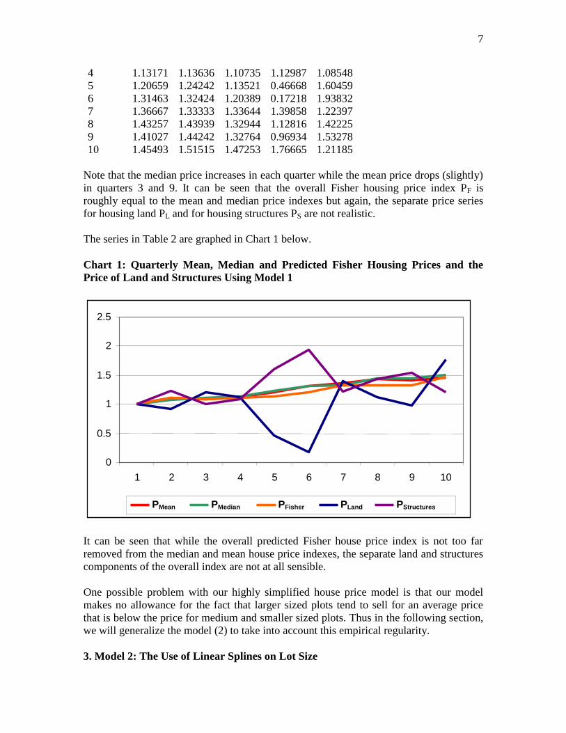
Table 3: Marginal Land Prices for Small, Medium and Large Lots, the Price of
Structures t and Decade Depreciation Rates
t
Quarter St
t L
t
t
t
1 0.31648 3.30552 0.87617 6.17826 0.06981
2 0.79113 2.96475 0.78643 6.44827 0.13999
3 1.77147 2.57100 1.27783 4.96547 0.12411
4 0.49927 3.48688 1.02879 6.61768 0.09022
5 0.59573 3.01473 0.44064 7.39286 0.13002
6 0.08365 3.81462 0.2504 8.38993 0.09269
7 1.09346 4.12335 1.26155 6.84204 0.09168
8 2.44028 3.06473 1.29751 5.71713 0.14456
9 2.00417 3.88380 0.88777 6.38234 0.14204
10 3.04236 3.33855 2.30271 5.49038 0.20080
Obviously, the estimated prices are not sensible; in particular, it is not likely that the cost
of an extra unit of land for a large plot could be negative in quarter 6!
Looking at the median price of a house over the 10 quarters in our sample, it was noted
earlier that the median price never fell over the sample period. This fact suggests that we
should impose this condition on all of our prices; i.e., we should set up a nonlinear
regression where the marginal prices of land never fall from quarter to quarter and where
the price of a square meter of a new structure also never falls. We will do this in the
following section and we will also impose a single depreciation rate over our sample
period, rather than allowing the depreciation rate to fluctuate from quarter to quarter.
4. Model 3: The Use of Monotonicity Restrictions on the Price of Land and
Structures
For the model to be described in this section, the data for all 10 quarters were run in one
big nonlinear regression. The equations that describe the model in quarter 1 are the same
as equations (3), (4) and (5) in the previous section except that the quarter one
depreciation rate parameter, 1, is replaced by the parameter , which will be used in all
subsequent quarters. For the remaining quarters, equations (3), (4) and (5) can still be
used except that the parameters St, M
t, L
t and
t are set equal to their quarter 1
counterparts plus a sum of squared parameters where one squared parameter is added
each period; i.e., St, M
t, L
t and
t are reparameterized as follows:
(6) St = S
1 + (S2)
2 + ... + (St)
2 ; t = 2,3,...,T;
(7) Mt = M
1 + (M2)
2 + ... + (Mt)
2 ; t = 2,3,...,T;
(8) Lt = L
1 + (L2)
2 + ... + (Lt)
2 ; t = 2,3,...,T;
(9) t =
1 + (2)
2 + ... + (t)
2 ; t = 2,3,...,T;
(10) t = ; t = 2,3,....T.

10
Thus our new parameters S2,...,St; M2,...,Mt; L2,...,Lt and 2,...,t and their squares
enter equations (6)-(9). It can be seen that this reparameterization will prevent the
marginal price of each type of land from falling and it will also impose monotonicity on
the price of structures.
The results of the above reparameterized model were as follows: the quarter 1 estimated
parameters were S1 = 0.56040 (0.24451), M
1 = 3.4684 (0.11304), L
1 = 0.33729
(0.04310), 1 = 6.2987 (0.39094) and = 0.11512 (0.006664), (standard errors in
brackets) with an R2 of .8439. Thus the overall decade depreciation rate was a very
reasonable 11.5% and the other parameters seemed to be reasonable in magnitude as well.
The only mild surprise was the fact that, at the beginning of the sample period, the
marginal valuation of land for small plots was 0.5604 while the marginal valuation for
medium plots was 3.4684 which was over 6 times as big. Thus small plots of land
suffered a discount in price per meter squared as compared to medium plots of land, at
least at the beginning of the sample period.14
Of the 36 squared parameters that pertain to
quarters 2 to 10, 23 were set equal to 0 by the nonlinear regression and only 13 were
nonzero with only 8 of these nonzero parameters having t statistics greater than 2. The
quarter by quarter values of the parameters St M
t L
t and
t defined by (6)-(9) are
reported in Table 4 below.
Table 4: Marginal Prices of Land for Small, Medium and Large Plots and New
Construction Prices by Quarter
Quarter St
t L
t
t
1 0.56040 3.46843 0.33729 6.29869
2 0.56040 3.46843 0.33729 6.42984
3 0.69803 3.46843 0.33729 6.42984
4 0.69803 3.46843 0.33729 6.72520
5 0.75139 3.46843 0.33729 6.80488
6 1.16953 3.46843 0.33729 6.80488
7 1.45453 3.62075 1.10353 6.80488
8 1.52233 3.62075 1.10353 6.80488
9 1.67159 3.62075 1.10353 6.80488
10 1.80029 3.62075 1.85418 6.80488
The above results look reasonable. The imputed price of new construction, t, was
approximately equal to 6.3 to 6.8 over the sample period (this translates into a price of
630 to 680 Euros per meter squared of structure floor space).15
The imputed value of land
14
This may not be a “genuine” effect; it is likely that the quality of construction is lower on small plots as
compared to the quality of medium and larger plots and since we are not taking this possibility into account
in our model, the lower average quality of structures on small plots may show up as a lower price of land
for small plots. We note also that by the end of the sample period, the difference in price was greatly
reduced. 15
Thus the imputed structures value of a new house with a floor space area of 125 meters squared would be
approximately 78,000 to 85,000 Euros.

11
for a small lot grew from 56 Euros per meter squared in the first quarter of 1998 to 180
Euros per meter squared in the second quarter of 2000. The imputed marginal value of
land16
for a lot size in the range of 200 to 400 meters squared grew very slowly from 347
Euros per meter squared to 362 Euros per meter squared over the same period. Finally,
the imputed marginal value of land17
for a lot size greater than 400 meters squared grew
very rapidly from 34 Euros per meter squared to 185 Euros per meter squared over the
sample period.
It is possible to work out the total imputed value of structures transacted in each quarter,
VSt, and divide this quarterly value by the total quantity of structures (converted into
equivalent new structure units), QSt, in order to obtain an average price of structures, PS
t.
Similarly, we can add up all of the imputed values for small, medium and large plot sizes
for each quarter t, say VLSt, VLM
t and VLL
t, and then add up the total quantity of land
transacted in each of the three classes of property, say QLSt, QLM
t and QLL
t. Finally, we
can form quarterly unit value prices for each of the three classes of property, PLSt, PLM
t
and PLLt, by dividing each value series by the corresponding quantity series. The resulting
price and quantity series are listed in Table 5 below.
Table 5: Average Prices for New Structures, Small, Medium and Large Plots and
Total Quantities Transacted per Quarter of Structures and the Three Types of Plot
Size
Quarter PSt
PLSt
PLMt PLL
t QS
t QLS
t QLM
t QLL
t
1 6.29869 0.56040 1.30977 1.17342 175.3 157.0 150.9 72.2
2 6.42984 0.56040 1.45836 1.43272 178.6 141.7 150.5 134.7
3 6.42984 0.69803 1.34450 1.42435 114.4 86.5 104.4 57.8
4 6.72520 0.69803 1.40970 1.25648 126.2 98.4 118.4 68.4
5 6.80488 0.75139 1.50785 1.22108 160.7 111.5 166.3 112.3
6 6.80488 1.16953 1.80168 1.37578 165.2 99.3 190.3 129.8
7 6.80488 1.45453 2.07368 1.97986 139.7 103.6 134.4 130.9
8 6.80488 1.52233 2.10779 1.84929 138.8 89.6 155.3 102.4
9 6.80488 1.67159 2.18339 1.92254 154.8 114.4 151.9 90.4
10 6.80488 1.80029 2.32405 2.38487 179.3 123.4 207.8 71.0
Note that the price of new structures series, PSt, and the price of land for small plots, PLS
t,
in Table 5 coincides with the series of values for t and S
t listed in Table 4. However,
the average prices for land in medium size plots, PLMt, and for large size plots, PLL
t, listed
in Table 5 no longer coincide with the corresponding marginal prices Mt and L
t listed in
Table 4. This is understandable since we have used splines to model how the price of a
meter squared of land varies as the lot size varies. Note that PLMt shows a much greater
rate of price increase over the sample period than the corresponding marginal price series
Mt, which hardly changed over the sample period. This is due to the fact that our model
16
This is our estimate of the value of an extra square meter of land above the threshold of 200 meters
squared (and below the threshold of 400 meters squared). 17
This is our estimate of the value of an extra square meter of land above the threshold of 400 meters
squared.

12
prices the first 200 meters squared of a medium sized lot at the average price of a small
lot and the price of small lots increased quite rapidly over the sample period. Another
striking feature of Table 5 is the tendency for the prices of land for small, medium and
large lots to equalize over time; i.e., at the beginning of the sample period, the price per
meter squared of a small lot was 56 Euros, for a medium lot, 131 Euros and for a large lot,
117 Euros but by the end of the sample period, the prices were 180 Euros, 232 Euros and
238 Euros, which was a considerable relative compression in the dispersion of these
prices. A final feature of Table 5 that should be mentioned is the tremendous volatility in
the quantities transacted in each quarter.
The four price series, PSt, PLS
t, PLM
t and PLL
t, were all normalized to equal unity in quarter
1 and they are plotted in Chart 2 below.
Chart 2: Prices For Structures PSt and for Three Sizes of Plot PLS
t, PLM
t and PLL
t
The data listed in Table 5 were further aggregated. We constructed a chained Fisher
aggregate for the three land series and the resulting aggregate land price and quantity
series, PLt and QL
t, are listed in Table 6 below along with the structures price and quantity
series (normalized so that the price equals 1 in quarter 1), PSt and QS
t. Finally, a chained
Fisher aggregate for structures and the three land series was constructed and the resulting
aggregate price and quantity series, Pt and Q
t, are also listed in Table 6.
Table 6: Aggregate Quarterly Price and Quantity Series for Housing
Quarter Pt PL
t PS
t Q
t QL
t QS
t
1 1.00000 1.00000 1.00000 1474.7 370.3 1104.3
2 1.04762 1.12142 1.02082 1565.6 438.6 1124.8
3 1.04778 1.12192 1.02082 972.1 252.3 720.6
4 1.07911 1.10969 1.06771 1084.5 289.8 794.9
0
0.5
1
1.5
2
2.5
3
3.5
1 2 3 4 5 6 7 8 9 10
PS PLS PLM PLL

13
5 1.10135 1.15701 1.08036 1421.3 407.7 1012.3
6 1.18041 1.42615 1.08036 1492.7 447.0 1040.9
7 1.29081 1.79379 1.08036 1270.1 383.9 880.0
8 1.28785 1.78392 1.08036 1240.6 366.1 874.3
9 1.31420 1.87589 1.08036 1331.6 371.3 975.0
10 1.36883 2.07249 1.08036 1530.3 421.9 1129.7
Finally, Chart 3 below plots the aggregate house price series Pt, the land price series PL
t
and the structures price series PSt from Table 6 above along with the quarterly mean price
series PMeant and median series PMedian
t.
Chart 3: Quarterly Mean Price PMeant, Median Price PMedian
t, Constant Quality
Housing Price Pt, Land Price PL
t and New Structures Price PS
t
From Chart 3, it is evident that our estimated constant quality price of housing for City A
grew more slowly than the corresponding mean and median series. The major
explanatory factor for this difference is probably due to the fact that the average age of
the structure in the quarterly sample tended to fall as time marched on.18
We have used only 3 characteristics of the property sales: the age of the structure, the
area of the land and the floor space area of the house. Real estate data bases generally
have information on many other characteristics of the house and these characteristics
could be integrated into the above hedonic framework.
18
The time series of average age by quarter in our sample was as follows: 1.38, 1.30, 1.24, 1.06, 1.19, 1.21,
1.16, 1.10, 0.957 and 1.18. The average amount of land tended to increase a bit over time; the quarterly
averages were as follows: 2.30, 2.60, 2.35, 2.48, 2.69, 2.80, 2.75, 2.78, 2.57 and 2.50. The average structure
size transacted by quarter was fairly steady: 1.26, 1.28, 1.26, 1.24, 1.28, 1.27, 1.20, 1.26, 1.24 and 1.29.
0
0.5
1
1.5
2
2.5
1 2 3 4 5 6 7 8 9 10
PMean PMedian P PL PS

14
In the following section, we will attempt to implement the model explained in this section
using monthly data in place of quarterly data.
5. A Monthly Model Using Monotonicity Restrictions
Before we repeat the Tables that were listed in the previous section using monthly data
instead of quarterly data, it is useful to list the descriptive statistics that describe the
monthly data. Thus in Table 7 below, we list various averages for the 30 months of data
in our sample as well as N, the number of observations in each month, which range from
a low of 26 in month 9 to a high of 63 in month 3.
Table 7: Descriptive Statistics for the Monthly Data
Month N Mean Median L S A fS fM fL
1 55 8.81447 7.4874 2.24109 1.27873 1.45455 0.63636 0.30909 0.05455
2 47 8.59045 7.4420 2.31872 1.21979 1.34043 0.61702 0.34043 0.04255
3 63 9.32068 7.7143 2.34635 1.28254 1.33333 0.57143 0.36508 0.06349
4 46 9.55868 7.7188 2.31326 1.30609 1.26087 0.56522 0.34783 0.08696
5 57 9.60040 7.9412 2.37298 1.24860 1.19298 0.63158 0.26316 0.10526
6 61 10.73692 9.4386 3.03672 1.29590 1.44262 0.45902 0.34426 0.19672
7 42 10.60333 8.4290 2.65738 1.28452 1.11905 0.47619 0.40476 0.11905
8 38 8.74363 8.1680 2.10316 1.24711 1.36842 0.52632 0.42105 0.05263
9 26 9.46656 8.4516 2.19615 1.25500 1.26923 0.65385 0.26923 0.07692
10 37 8.94806 8.1680 2.30027 1.18405 1.24324 0.54054 0.43243 0.02703
11 41 10.96991 8.6218 2.79439 1.27293 1.00000 0.53659 0.34146 0.12195
12 37 10.35631 8.8487 2.31162 1.26081 0.94595 0.54054 0.37838 0.08108
13 51 10.44940 9.3025 2.98471 1.23941 1.43137 0.47059 0.47059 0.05882
14 40 10.12645 8.1680 2.35350 1.28575 1.07500 0.62500 0.25000 0.12500
15 54 11.60774 10.4256 2.66296 1.30981 1.03704 0.40741 0.48148 0.11111
16 40 11.18432 11.1176 2.61050 1.25925 1.35000 0.45000 0.50000 0.05000
17 53 11.49708 9.5385 3.04830 1.27453 1.05660 0.45283 0.37736 0.16981
18 57 12.40321 10.7319 2.69088 1.28018 1.26316 0.38596 0.50877 0.10526
19 46 12.09197 10.3258 2.69978 1.23217 1.26087 0.47826 0.36957 0.15217
20 37 12.28354 9.9378 2.74324 1.18595 1.05405 0.56757 0.29730 0.13514
21 51 12.29845 10.0966 2.80902 1.18529 1.15686 0.45098 0.39216 0.15686
22 36 11.45179 10.4483 2.53528 1.19500 1.41667 0.47222 0.47222 0.05556
23 43 12.75577 10.1647 2.88791 1.27116 1.09302 0.51163 0.34884 0.13953
24 46 13.93129 11.9968 2.86565 1.31087 0.84783 0.36957 0.52174 0.10870
25 36 12.96740 10.8226 2.76778 1.28361 0.80556 0.52778 0.33333 0.13889
26 50 12.95475 10.8453 2.68940 1.24160 1.04000 0.48000 0.44000 0.08000
27 53 12.05086 10.5504 2.31226 1.21755 0.98113 0.52830 0.41509 0.05660
28 61 12.17228 10.7773 2.32656 1.26246 1.21311 0.54098 0.40984 0.04918
29 50 13.33456 10.6638 2.69700 1.31660 1.22000 0.42000 0.48000 0.10000
30 50 13.71641 12.7625 2.50760 1.30640 1.10000 0.44000 0.50000 0.06000
It can be seen that the monthly means and medians no longer steadily trend upwards;
there are now many ups and downs in these series. The L and S series are the monthly
average amounts of land and structures (in 100s of square meters) sold in each month.
15
There are large fluctuations in some of these averages: L ranges from a low of 2.10 to a
high of 3.05 while S ranges from 1.18 to 1.32. The average age in decades, A, ranges
from a low of 0.81 to 1.45. The fraction of small lots transacted in a given month, fS,
ranges from a low of 0.370 to a high of 0.654; the fraction of medium sized lots
transacted in a given month, fM, ranges from a low of 0.250 to a high of 0.522 and the
fraction of large lots transacted in a given month, fL, ranges from a low of 0.027 to a high
of 0.197. Given the magnitude of these fluctuations, it can be seen that it is unreasonable
to expect the mean and median series to give a good approximation to pure price change
because the underlying monthly characteristics are changing so dramatically from month
to month (and so the mean and median series embody quantity effects as well as price
effects).
The model described in the previous section was rerun using the monthly data so that we
now have 30 monthly time periods in place of the old 10 quarterly time periods. The
number of parameters to be estimated has skyrocketed to 121 from the old 41 parameters.
The results for the monthly model were as follows: the month 1 estimated parameters
were S1 = 0.60606 (0.23277), M
1 = 3.3440 (0.11841), L
1 = 0.32289 (0.04100),
1 =
6.1899 (0.40215) and = 0.11603 (0.00717) (standard errors in brackets) with an R2
of .8509. Recall that the corresponding quarterly model parameters for quarter 1 were:
S1 = 0.56040 (0.24451), M
1 = 3.4684 (0.11304), L
1 = 0.33729 (0.04310),
1 = 6.2987
(0.39094) and = 0.11512 (0.00666), (standard errors in brackets) with an R2 of .8439.
Thus the monthly model has generated parameter estimates that are quite similar to the
quarterly model. Of the 116 squared parameters that pertain to months 2 to 30, 97 were
set equal to 0 by the nonlinear regression and only 19 were nonzero with 7 of these
nonzero parameters having t statistics greater than 2. The month by month values of the
parameters St M
t L
t and
t defined by (6)-(9) are reported in Table 8 below.
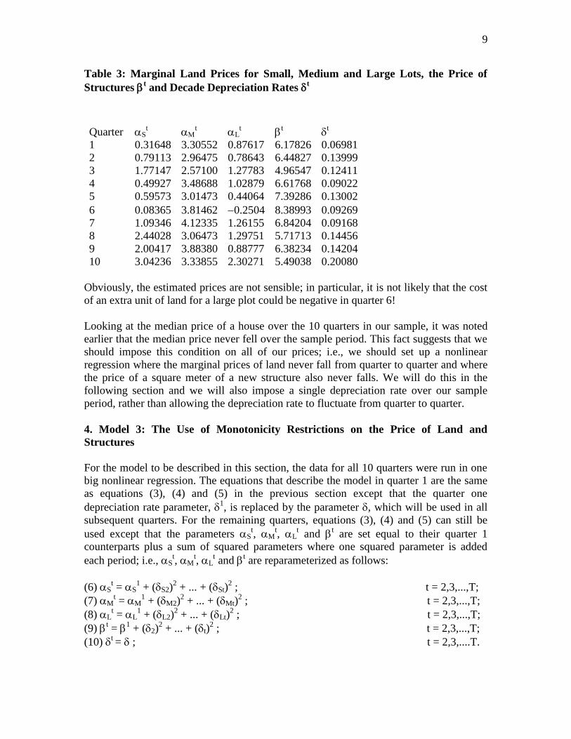
Table 8: Marginal Prices of Land for Small, Medium and Large Plots and New
Construction Prices by Month
Month St
t L
t
t
1 0.60606 3.34397 0.32289 6.18992
2 0.60606 3.34397 0.32289 6.27455
3 0.60606 3.34397 0.32289 6.30662
4 0.60606 3.34397 0.32289 6.30662
5 0.73532 3.34397 0.32289 6.30662
6 0.73532 3.34397 0.32289 6.30662
7 0.79559 3.34397 0.32289 6.30662
8 0.79559 3.34397 0.32289 6.30662
9 0.79559 3.34397 0.32289 6.30662
10 0.79559 3.34397 0.32289 6.30662
11 0.79559 3.34397 0.32289 6.74011
12 0.79559 3.34397 0.32289 6.74011
13 0.79559 3.34397 0.32289 6.74011
14 0.79559 3.34397 0.32289 6.74011
15 0.95792 3.34397 0.32289 6.74633

16
16 0.97205 3.34397 0.32289 6.74633
17 0.97205 3.34397 0.32289 6.74633
18 1.41488 3.64341 1.05297 6.74633
19 1.41488 3.64341 1.05297 6.74633
20 1.54421 3.64341 1.05297 6.74633
21 1.54421 3.64341 1.05297 6.74633
22 1.54421 3.64341 1.05297 6.74633
23 1.54421 3.64341 1.05297 6.74633
24 1.62185 3.64341 1.05297 6.74633
25 1.62185 3.64341 1.05297 6.74633
26 1.64154 3.64341 1.48534 6.74633
27 1.74104 3.64341 1.48534 6.74633
28 1.74104 3.64341 1.83463 6.74633
29 1.74104 3.64341 1.83463 6.74633
30 1.95408 3.79082 3.60152 6.74633
25 1.62185 3.64341 1.05297 6.74633
26 1.64154 3.64341 1.48534 6.74633
27 1.74104 3.64341 1.48534 6.74633
28 1.74104 3.64341 1.83463 6.74633
29 1.74104 3.64341 1.83463 6.74633
30 1.95408 3.79082 3.60152 6.74633
Comparing the entries in Table 8 with the corresponding quarterly entries in Table 4, it
can be seen that the monthly results agree fairly well with the quarterly results with the
exception of the sudden surge in the marginal price for large lots in month 30 of Table 8
from 1.83 in month 29 to 3.60 in month 30. This discrepancy could be due to the fact that
the fraction of large lots sold is rather small and so the estimate of the marginal price of
large lots is particularly uncertain. Another possible explanation for the large surge in the
marginal price for large lots in both the quarterly and monthly models is the fact that
nonparametric time series models tend to be unreliable at the endpoints of the sample
period because there is a tendency for the model to fit the errors at the endpoints. Our
model is very close to being a nonparametric time series model since it has many free
parameters for each time period and thus, it may be subject to this type of bias.19
As in the previous section, it is possible to work out the total imputed value of structures
transacted in each month, VSt, and divide this monthly value by the total quantity of
structures (converted into equivalent new structure units), QSt, in order to obtain an
average price of structures, PSt. Similarly, we can add up all of the imputed values for
small, medium and large plot sizes for each month t, say VLSt, VLM
t and VLL
t, and then
add up the total quantity of land transacted in each of the three classes of property, say
QLSt, QLM
t and QLL
t. Finally, we can form monthly unit value prices for each of the three
classes of property, PLSt, PLM
t and PLL
t, by dividing each value series by the
corresponding quantity series. The resulting (average) price and quantity series are listed
in Table 9 below.
19
This hypothesis could be checked by adding some additional months of data to the original sample.

17
Table 9: Average Prices for New Structures, Small, Medium and Large Plots and
Total Quantities Transacted per Month of Structures and the Three Types of Plot
Size
Month PSt
PLSt
PLMt PLL
t QS
t QLS
t QLM
t QLL
t
1 6.18992 0.60606 1.34892 1.23190 58.3 54.8 46.7 21.8
2 6.27455 0.60606 1.19025 0.88222 48.7 44.7 40.7 23.6
3 6.30662 0.60606 1.36185 1.31034 68.1 57.5 63.5 26.8
4 6.30662 0.60606 1.39050 1.54612 51.3 40.0 44.8 21.6
5 6.30662 0.73532 1.54738 1.47993 61.1 56.1 43.6 35.6
6 6.30662 0.73532 1.57825 1.38603 65.9 45.7 62.0 77.5
7 6.30662 0.79559 1.42916 1.31151 46.7 31.0 45.3 35.3
8 6.30662 0.79559 1.30271 1.70519 40.0 29.9 40.0 10.1
9 6.30662 0.79559 1.48092 1.45265 27.5 25.6 19.1 12.4
10 6.30662 0.79559 1.43238 0.97532 37.6 31.7 42.7 10.7
11 6.74011 0.79559 1.51717 1.17130 46.5 34.3 39.1 41.2
12 6.74011 0.79559 1.39970 1.59412 46.5 35.8 40.7 18.3
13 6.74011 0.79559 1.54564 0.77613 52.7 38.0 68.0 46.3
14 6.74011 0.79559 1.47085 1.58783 44.9 39.3 27.2 27.6
15 6.74633 0.95792 1.59816 1.46394 62.9 34.3 71.1 38.5
16 6.74633 0.97205 1.71434 1.15279 42.7 28.5 58.2 17.7
17 6.74633 0.97205 1.60087 1.25917 59.8 36.6 54.4 70.6
18 6.74633 1.41488 1.97969 1.90646 62.6 34.2 77.7 41.5
19 6.74633 1.41488 2.06124 2.04227 48.8 34.5 47.9 41.8
20 6.74633 1.54421 2.18701 1.91885 38.6 34.2 31.7 35.6
21 6.74633 1.54421 2.11170 1.97373 52.1 34.9 54.8 53.6
22 6.74633 1.54421 2.04024 1.69432 35.7 27.5 44.5 19.2
23 6.74633 1.54421 2.14576 1.83314 48.2 34.7 42.1 47.4
24 6.74633 1.62185 2.23240 1.93694 54.8 27.3 68.8 35.7
25 6.74633 1.62185 2.09679 1.87980 41.9 30.1 31.4 38.2
26 6.74633 1.64154 2.22615 2.01935 55.4 37.6 62.2 34.7
27 6.74633 1.74104 2.20914 2.31150 57.4 46.7 58.4 17.5
28 6.74633 1.74104 2.23174 2.39151 65.9 56.1 67.4 18.5
29 6.74633 1.74104 2.25524 2.29521 56.7 31.8 65.8 37.2
30 6.74633 1.95408 2.56009 3.02895 56.5 35.5 74.6 15.3
Comparing the monthly prices in Table 9 with their quarterly counterparts in Table 5, it
can be seen that the prices of structures and the (average) prices of small lots are very
similar in the two tables. However, there are some substantial differences between the
quarterly and monthly average prices of medium and large lots. Moreover, in both tables,
it can be seen that there are some fluctuations in the average prices of medium and large
lots, with the fluctuations being quite substantial in the case of monthly prices. These
fluctuations are due to the smaller sample sizes in the monthly model compared to the
quarterly model and to the nature of our spline model for the cost of land. The marginal
price of land for an extra unit of land for a medium lot is greater than the marginal price
for an extra unit of land for a small lot. Thus if the average size of a medium lot increases

18
going from one period to the next, then the average price for medium lots will increase.
Similarly, the marginal price of land for large lots is less than the marginal price for
medium lots. Thus if the average size of a large lot increases going from one period to the
next, then the average price for large lots will decrease. Since monthly sample sizes can
be small for medium and large lots, substantial fluctuations in the average size of lots
sold in each month within these two categories of lot size will lead to substantial
fluctuations in the average prices for these two types of lot.20
This type of fluctuation can
be controlled by making the lot size ranges smaller so that divergences between marginal
and average prices within each lot size category would be reduced.21
Another method for
controlling these spline model induced fluctuations would be to drop the spline model for
the price of land and simply have one price of land for all lot sizes. However, we are
reluctant to do this since our results for the Dutch city “A” indicate that the price levels
and trends for the different sized lots differed substantially.
A final method for controlling spline model induced fluctuations in the price of land
would be to value the entire stock of detached houses in the city using our model. Since
the stock of houses changes very little from month to month, this would eliminate large
fluctuations in the average amount of land for medium and large lots.22
We note that our model could serve many purposes. As indicated in the above paragraph,
the model could be used to provide up to date valuations for the entire stock of detached
houses in the city, provided that we had information on the age, land area and floor space
area for each house in the city. The model could also be used to value new additions to
the city‟s housing stock provided that information on the age, land area and floor space
area for each newly constructed house in the city was available.23
The data listed in Table 9 were further aggregated. We constructed a chained Fisher
aggregate for the three land series and the resulting aggregate land price and quantity
series, PLt and QL
t, are listed in Table 10 below along with the structures price and
quantity series (normalized so that the price equals 1 in quarter 1), PSt and QS
t. Finally, a
20
Analogous fluctuations for small lots (and for structures) cannot occur because for these commodities,
average and marginal prices coincide. 21
A possible problem with this strategy is that the sample sizes within each category of lot would decline
and become zero in some cases. However, this is not necessarily a problem since our spline model does not
really require that the sample size within each lot size category be nonzero; i.e., our spline model shifts the
entire schedule of lot size costs up (or down if we entered the squared terms in equations (6)-(8) into the
model with negative signs instead of positive signs) and we do not require actual transactions in a given
period for all possible lot sizes. Thus the main cost of increasing the number of spline segments appears to
be the fact that a large number of additional parameters would have to be estimated. 22
This is our preferred method for controlling price fluctuations due to the changing composition of the
houses sold from period to period. However, this method requires information on the total stock of housing
for the neighbourhood under consideration. Alternatively, one could simply use the characteristics of a
“representative” dwelling unit for the neighbourhood. 23
If the country uses the acquisitions approach to the treatment of housing in a Consumer Price Index
where only the price of the new structure is to enter the index, then it can be seen that our suggested model
could be very useful in this context. For a review of alternative ways of treating housing in a CPI, see
Diewert (2002; 611-121) (2007).

19
chained Fisher aggregate for structures and the three land series were constructed and the
resulting aggregate price and quantity series, Pt and Q
t, are also listed in Table 10.
Table 10: Aggregate Monthly Price and Quantity Series for Housing
Month Pt PL
t PS
t Q
t QL
t QS
t
1 1.00000 1.00000 1.00000 483.6 123.0 360.6
2 0.97671 0.87263 1.01367 411.5 110.4 301.5
3 1.02074 1.02282 1.01885 574.1 153.0 421.6
4 1.03527 1.07812 1.01885 428.5 111.3 317.7
5 1.05917 1.16874 1.01885 516.4 138.1 378.5
6 1.05293 1.14866 1.01885 621.4 208.0 407.7
7 1.03402 1.08904 1.01885 416.1 124.6 289.1
8 1.04220 1.11502 1.01885 331.2 83.4 247.5
9 1.04970 1.14454 1.01885 229.0 58.3 170.5
10 1.02374 1.04618 1.01885 326.5 92.5 233.1
11 1.09622 1.12517 1.08888 408.6 119.8 287.5
12 1.11565 1.19293 1.08888 383.7 96.0 287.9
13 1.07571 1.06179 1.08888 489.5 161.3 326.3
14 1.13645 1.27653 1.08888 367.4 90.2 277.7
15 1.155 1.34473 1.08989 543.1 150.7 389.5
16 1.15423 1.34156 1.08989 377.5 110.3 264
17 1.1492 1.32413 1.08989 535.3 159.8 370.3
18 1.29115 1.80736 1.08989 544.8 155.6 387.3
19 1.31333 1.8846 1.08989 428.2 123.6 302.3
20 1.32546 1.92648 1.08989 339.9 98.9 238.7
21 1.32357 1.92014 1.08989 473.8 143.4 322.8
22 1.28999 1.80714 1.08989 315.1 91.8 220.7
23 1.31473 1.89256 1.08989 422.7 121.9 298.1
24 1.34044 1.98243 1.08989 475.2 134.7 339.4
25 1.3194 1.90712 1.08989 355.3 97.7 259.2
26 1.3477 2.00881 1.08989 477.8 134.5 342.9
27 1.37051 2.09286 1.08989 465.4 119.8 355.2
28 1.37623 2.11508 1.08989 535.5 138.1 408.2
29 1.37396 2.10695 1.08989 488.8 137.3 350.8
30 1.47345 2.46897 1.08989 466.9 124.2 349.8
10 1.36883 2.07249 1.08036 1530.3 421.9 1129.7
Comparing the monthly price series in Table 10 with the corresponding quarterly price
series in Table 6, it can be seen that they are reasonably close except that monthly price
of land averaged over the last 3 months is 2.23 which is somewhat above the
corresponding quarterly land index for the last quarter which was 2.07. The monthly
price of structures for the last 3 months was steady at 1.09 which corresponds closely to
the quarterly price of structures for the last quarter, which was 1.08. As mentioned above,
we believe the quarterly results are likely to be more reliable.

20
Chart 4 below plots the monthly aggregate house price series Pt, the land price series PL
t
and the structures price series PSt from Table 10 above along with the monthly mean
price series PMeant and median series PMedian
t.
Chart 4: Monthly Mean Price PMeant, Median Price PMedian
t, Constant Quality
Housing Price Pt, Land Price PL
t and New Structures Price PS
t
From Chart 4, it is evident that our estimated constant quality price of housing for City A
grew more slowly than the corresponding mean and median series. As was the case with
the quarterly Chart 3, the major explanatory factor for this difference is due to the fact
that the average age of the structure in the sample tended to fall as time marched on.
It is of interest to take the monthly data from Table 9 and aggregate these data into
quarterly unit value prices and the corresponding quarterly quantities. This was done,
generating three aggregated quarterly land price and quantity series and the aggregated
quarterly structures price series, APSt. These three aggregated land price series were then
aggregated into an overall aggregated quarterly price series APLt using chained Fisher
aggregation. Finally, the three aggregated land price series and the aggregated constant
quality structures series APSt were aggregated into an overall aggregated quarterly
housing price index, APt, which is listed in Table 11 below along with APL
t and APS
t. For
comparison purposes, the corresponding quarterly price series for housing, land and
structures, Pt, PL
t and PS
t, from Table 6 in section 4 (i.e., the estimates from the original
quarterly regression model) are also listed in Table 11.
Table 11: Quarterly Price Series for Housing Pt, Land PL
t and for Structures PS
t
and Aggregated Quarterly Price Series for Housing APt, Land APL
t and for
Structures APSt from the Monthly Model
0
0.5
1
1.5
2
2.5
3
1 2 3 4 5 6 7 8 9 10 11 12 13 14 15 16 17 18 19 20 21 22 23 24 25 26 27 28 29 30
PMean PMedian P PL PS

21
Quarter APt APL
t APS
t P
t PL
t PS
t
1 1.00000 1.00000 1.00000 1.00000 1.00000 1.00000
2 1.05456 1.18206 1.00763 1.04762 1.12141 1.02082
3 1.04880 1.16087 1.00763 1.04778 1.12192 1.02082
4 1.08160 1.14810 1.05693 1.07912 1.10971 1.06771
5 1.10979 1.19665 1.07728 1.10135 1.15704 1.08036
6 1.17932 1.43075 1.07788 1.18040 1.42616 1.08036
7 1.29550 1.81536 1.07788 1.29081 1.79380 1.08036
8 1.29277 1.80633 1.07788 1.28785 1.78395 1.08036
9 1.31920 1.89783 1.07788 1.31421 1.87592 1.08036
10 1.37667 2.10340 1.07788 1.36883 2.07254 1.08036
The above series are graphed in Chart 5 below.
Chart 5: Quarterly Constant Quality Housing Price Pt, Land Price PL
t and New
Structures Price PSt and the Corresponding Quarterly Aggregates Generated by the
Monthly Model, APt, APL
t and APS
t
It can be seen that the original quarterly overall house price index series, P
t, coincides so
closely with the corresponding aggregated series from the monthly model, APt, that the
two series can barely be distinguished from each other in Chart 5. Similarly the original
quarterly constant quality structures price index, PSt, can barely be distinguished from its
aggregated counterpart from the monthly model, APSt. Finally, the original quarterly
0
0.5
1
1.5
2
2.5
1 2 3 4 5 6 7 8 9 10
AP APL APS P PL PS
22
series for land, PLt, lies slightly below its monthly aggregated counterpart, APL
t. Our
conclusion is that the monthly and quarterly hedonic regression models are in fairly close
agreement with each other. Both models seem to give sensible results.
It can be seen that the logic behind our functional form assumptions for our hedonic
regression model come from the supplier perspective; i.e., we justified our model from
the perspective of a builder who buys a lot at a given price per squared meter and then
builds a structure on the lot at another price per squared meter of floor space of the
structure.24
But it is important to justify a hedonic regression model from a consumer or
purchaser perspective as well25
and in the following section, we explore such an approach.
6. Hedonic Regressions for Housing from a Consumer Perspective
A very simple way to justify a hedonic regression model from a consumer perspective is
to postulate that households have the same (cardinal) utility function, f(z1,z2), that
aggregates the amounts of two relevant characteristics, z1 > 0 and z2 > 0, into the overall
utility of the “model” with characteristics z1, z2 into the scalar welfare measure, f(z1,z2).
Thus households will prefer model 1 with characteristics z11,z2
1 to model 2 with
characteristics z12,z2
2 if and only if f(z1
1,z2
1) > f(z1
2,z2
2).
26 Thus having more of every
characteristic is always preferred by households. The next assumption that we make is
that in period t, there is a positive generic price for all models, t, such that the
household‟s willingness to pay, Wt(z1,z2), for a model with characteristics z1 and z2 is
equal to the generic model price t times the utility generated by the model, f(z1,z2); i.e.,
we have for each model n with characteristics z1nt, z2n
t that is purchased in period t, the
following willingness to pay for model n:27
(11) Wt(z1n
t,z2n
t) =
t f(z1n
t,z2n
t).
In order to relate the above model to sales in the Dutch city of “A”, identify the first
characteristic with the size of the land area of the house n sold in period t, Lnt, and the
24
Thorsnes (1997) also takes a producer perspective but he assumed that developers have a CES production
function for housing services that are produced by combining land and structures inputs whereas we simply
assume that structures and land can be separately combined in an additive fashion. 25
Purchaser preferences for properties are perhaps more important than producer costs of production since
a property will not be purchased unless the utility of the property to the buyer is equal to or greater than its
cost. On the other hand, developers will not build new houses unless they cover their costs of production,
which argues for the importance of the producer perspective to hedonic regression models. Rosen (1974)
argues for the importance of both sides of the market. In terms of Rosen‟s analysis of the determinants of
the hedonic surface, for the production of new houses, we would argue that we are in his Case 1 where cost
conditions are identical across firms and thus the hedonic surface is determined by the supply side of the
market; see Rosen (1974; 50-51). 26
It is natural to impose some regularity conditions on the characteristics aggregator function f like
continuity, monotonicity (if each component of the vector z1 is strictly greater than the corresponding
component of z2, then f(z
1) > f(z
2) and f(0,0) = 0. The hedonic housing model presented in this section is
essentially a variant of McMillen‟s (2003) model. 27
For more elaborate justifications for household based hedonic regression models, see Muellbauer (1974)
and Diewert (2003).

23
second characteristic with the quality adjusted (for the age of the structure) size of the
structure, ASnt, so that
(12) ASnt (1 A)Sn
t
where Snt is the unadjusted size of the structure, is the depreciation rate for structures
and A is the age of the structure. Finally, set the willingness to pay for the housing unit,
Wt(Ln
t,(1 A)Sn
t), equal to the selling price of the property, vn
t and we have the
following hedonic regression model:
(13) vnt =
t f(Ln
t,(1 A)Sn
t).
There remain the problems of choosing a stochastic specification for the hedonic
regression model (12) and of choosing a functional form for the hedonic utility function f.
The simplest choices for f(L,AS) are that (i) f is a linear function of L and AS or (ii) f has
a Cobb-Douglas functional form. These two choices lead to the following hedonic
regression models after adding mean zero error terms nt to each choice:
28
(14) vnt =
t(Ln
t + (1 An
t)Sn
t) + n
t ; n = 1,...,N(t); t = 1,...,T;
(15) lnvnt = ln
t + + lnLn
t + ln[(1 An
t)Sn
t] + n
t ; n = 1,...,N(t); t = 1,...,T.
In order to identify all of the parameters, we require a normalization on the hedonic
prices t. It is natural to set
t equal to one in the first period:
(16) 1 = 1.
It can be seen that the hedonic regression model defined by (14) and (16) is essentially a
reparameterization of our first simple regression model explained in section 2 above
(with some additional restrictions on the parameters). However, the Cobb-Douglas model
defined by (15) and (16) is a new model and we will use our 10 quarters of data in order
to estimate the nine time dummy parameters, 2,
3, ... ,
10, and the 4 remaining
parameters, , , and . This model is essentially a standard log-log time dummy
hedonic regression model.29
The results of the above Cobb-Douglas model were as follows: the quarter 1 estimated
parameters were = 1.7662 (0.016564), = 0.49941 (0.011127), = 0.50163 (0.024201)
and = 0.12609 (0.0072004) (standard errors in brackets) with an R2 of 0.8244.
30 The
parameters ln2, ln
3,..., ln
10 were 0.0376, 0.0265, 0.0034, 0.0496, 0.0669, 0.0554,
28
Note that the linear f(L,AS) that is defined in (14) is linearly homogeneous in the variables L and AS.
The Cobb-Douglas f that is defined in (15) will be linearly homogeneous if + = 1. McMillen‟s (2003)
hedonic housing model that uses a consumer perspective is essentially the Cobb-Douglas model defined by
(15). 29
The only unusual feature of this model is the nonlinearity that arises from the use of quality adjusted
structures as a characteristic rather than the use of unadjusted structures and age as explanatory variables. 30
Recall that in the quarterly model estimated in section 4, the R2 was .8439 and the estimated depreciation
rate was 0.11512 which is a bit lower than our present estimated decade depreciation rate of 0.12609.

24
0.0217, 0.0161 and 0.0314 respectively and the standard errors for all of these time
dummy variables was very close to 0.02. Thus the estimate for the quarter 4 time dummy,
ln4, turned out to be negative but it was not significantly negative since the t statistic
was only 0.15.
The most interesting feature of our quarterly log-log regression is that our estimated
Cobb-Douglas hedonic aggregator function exhibited virtually constant returns to scale
in the two characteristics; i.e., our parameter estimates for and summed to 1.00104.31
Our estimated time dummy variables were exponentiated and are reported as the t series
in Table 12 below.32
These estimated overall house price indexes can be compared with
our earlier estimates listed in Table 6 above; see the series Pt listed there. It can be seen
that the correspondence between t and our earlier price series for housing P
t is fairly
close; see Chart 6 below.
We now encounter a problem with the log-log hedonic regression model as compared to
the linear hedonic regression model explained in section 4 above: the linear model
generated separate estimates for the price of land and for the price of quality adjusted
structures whereas the present model does not seem to be able to generate these separate
estimates for the price of land and structures. However, it is possible to use the log-log
model (or any other hedonic model based on a hedonic utility function f(z1,z2)) in order to
generate imputed estimates for the price of land, Lt, and for quality adjusted structures,
St. The basic idea is to take the consumer‟s period t willingness to pay function,
Wt(z1,z2), and differentiate it with respect to z1 and z2. These two partial derivatives will
give us estimates of the consumer‟s increase in well being in period t, valued at the
period t price for the hedonic aggregate, due to a marginal increase in the quantities of z1
and z2; i.e., we will have imputed prices for extra units of z1 and z2 in period t. Thus we
define Lt and S
t as follows:
(17) Lt W
t(z1
t*,z2
t*)/z1 =
tf(z1
t*,z2
t*)/z1 ; t = 1,...,T ;
(18) St W
t(z1
t*,z2
t*)/z2 =
tf(z1
t*,z2
t*)/z2 ; t = 1,...,T
where z1t*
and z2t*
are the average amounts of land and quality adjusted structures for the
properties sold in period t; see the last two columns of Table 12 for a listing of these
average quantities for our sample of 10 quarters of data. Note that the average amount of
land series is more volatile than the average quantity of quality adjusted structures series.
We use (17) and (18) to generate imputed price series for land and quality adjusted
structures, using our estimated coefficients for , and in order to form an estimated
31
We also estimated the log-linear variant of a hedonic regression; i.e., our estimating equation for this
model was lnvnt =
t(Ln
t + (1 An
t)Sn
t) + n
t. Our Dutch data did not support this model at all; the final
log likelihood for this model was only 226.33 as compared to the final log likelihood for the log-log model
of 587.27. The R2 for the log-linear model was only 0.7064 as compared to the R
2 of 0.8244 for the log-log
model. Both the log-linear and the log-log model have the same dependent variables so their log likelihoods
and R2 can be compared.
32 We set
1 = 1.
25
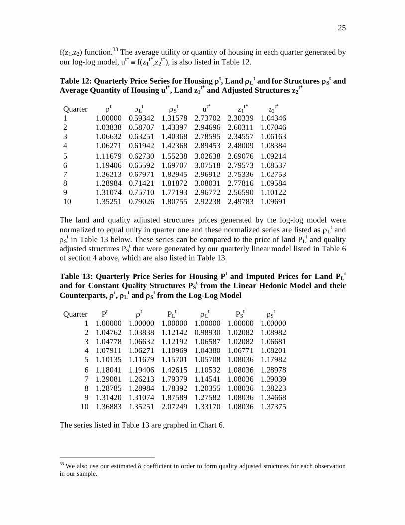
f(z1,z2) function.33
The average utility or quantity of housing in each quarter generated by
our log-log model, ut*
f(z1t*
,z2t*
), is also listed in Table 12.
Table 12: Quarterly Price Series for Housing t, Land L
t and for Structures S
t and
Average Quantity of Housing ut*
, Land z1t*
and Adjusted Structures z2t*
Quarter t
Lt S
t u
t* z1
t* z2
t*
1 1.00000 0.59342 1.31578 2.73702 2.30339 1.04346
2 1.03838 0.58707 1.43397 2.94696 2.60311 1.07046
3 1.06632 0.63251 1.40368 2.78595 2.34557 1.06163
4 1.06271 0.61942 1.42368 2.89453 2.48009 1.08384
5 1.11679 0.62730 1.55238 3.02638 2.69076 1.09214
6 1.19406 0.65592 1.69707 3.07518 2.79573 1.08537
7 1.26213 0.67971 1.82945 2.96912 2.75336 1.02753
8 1.28984 0.71421 1.81872 3.08031 2.77816 1.09584
9 1.31074 0.75710 1.77193 2.96772 2.56590 1.10122
10 1.35251 0.79026 1.80755 2.92238 2.49783 1.09691
The land and quality adjusted structures prices generated by the log-log model were
normalized to equal unity in quarter one and these normalized series are listed as Lt and
St in Table 13 below. These series can be compared to the price of land PL
t and quality
adjusted structures PSt that were generated by our quarterly linear model listed in Table 6
of section 4 above, which are also listed in Table 13.
Table 13: Quarterly Price Series for Housing Pt and Imputed Prices for Land PL
t
and for Constant Quality Structures PSt from the Linear Hedonic Model and their
Counterparts, t, L
t and S
t from the Log-Log Model
Quarter Pt
t PL
t L
t PS
t S
t
1 1.00000 1.00000 1.00000 1.00000 1.00000 1.00000
2 1.04762 1.03838 1.12142 0.98930 1.02082 1.08982
3 1.04778 1.06632 1.12192 1.06587 1.02082 1.06681
4 1.07911 1.06271 1.10969 1.04380 1.06771 1.08201
5 1.10135 1.11679 1.15701 1.05708 1.08036 1.17982
6 1.18041 1.19406 1.42615 1.10532 1.08036 1.28978
7 1.29081 1.26213 1.79379 1.14541 1.08036 1.39039
8 1.28785 1.28984 1.78392 1.20355 1.08036 1.38223
9 1.31420 1.31074 1.87589 1.27582 1.08036 1.34668
10 1.36883 1.35251 2.07249 1.33170 1.08036 1.37375
The series listed in Table 13 are graphed in Chart 6.
33
We also use our estimated coefficient in order to form quality adjusted structures for each observation
in our sample.

26
Looking at Table 13 and Chart 6, it can be seen that our overall estimates of house price
inflation from the linear hedonic model, Pt, and from the log-log hedonic model,
t, are
very close to each other. However, the two hedonic models produce very different
estimates of land and structures inflation: the estimates of land price inflation from the
linear model, PLt, are well above the corresponding log-log estimates, L
t, whereas the
estimates of structures price inflation from the linear model, PSt, are well below the
corresponding log-log estimates, St. The question naturally arises: which set of estimates
is closer to the “truth”?
Chart 6: Quarterly Price Series for Housing Pt and Imputed Prices for Land PL
t and
for Constant Quality Structures PSt and their Counterparts,
t, L
t and S
t
We believe that the estimates from the linear model are more credible. Evidently, there
was a bit of a house price “bubble” in the Netherlands during these 10 quarters. The log-
log model attributes more than half of the bubble to increases in the price of structures
whereas the linear model attributes most of the bubble to increases in the price of land. A
look at construction prices in the Netherlands shows that construction prices did not
increase dramatically during these 10 quarters starting at the first quarter of 1998.34
Thus
the linear model is more consistent with the actual pattern of construction prices and the
price of raw land during this period. One could argue that this is irrelevant: what counts
are household, or more generally, purchasers valuations of the characteristics and these
34
The Statistics Netherlands (national) Construction Price Index for new dwellings for the same period
took on the following values (with Q1 in 1998 normalized to equal unity): 100, 100.4, 100.4, 100.8, 101.0,
101.7, 102.7, 103.1, 104.5,105.1.
0
0.5
1
1.5
2
2.5
1 2 3 4 5 6 7 8 9 10
P PL L PS S

27
valuations do not have to coincide with market prices for units of the characteristics
purchased separately. However, a situation where a purchaser‟s valuation of an extra unit
of land is well below the market price of land and where the valuation of an extra unit of
structure is well above the market price of building that extra unit should not persist
indefinitely: there will be a tendency for purchasers to buy houses with more floor space
and less land in order to move their marginal willingness to pay for land and structures
closer to the corresponding market prices for land and structures.
7. Conclusion
Our tentative conclusion at this point is that hedonic regression techniques can be used in
order to decompose the selling prices of properties into their land and structure
components but it is not a completely straightforward exercise. In particular,
monotonicity restrictions on the parameters will generally have to be imposed on the
model in order to obtain sensible results35
We found that our model worked fairly well on
monthly data as well as on quarterly data. Our results also indicate that stable coefficients
cannot be obtained using just data for one quarter. An open question is: how many
quarters (or months) of data do we need to run in the one big nonlinear regression in
order to obtain stable imputed prices for land and structures?
Here is a list of topics where further research is required:
Can we adapt our method into a rolling year method; i.e., we use only the data for
a full year plus one additional time period and use the results to update our
previous series?36
We did not eliminate any outliers in our preliminary research. Do we get similar
results if outliers are eliminated?37
Is it worthwhile to consider more characteristics?
How does our suggested method compare to the repeat sales method38
(using the
same data set)?
Can our method be generalized to deal with the sales of condominiums and
duplexes?39
35
In our data set, it was reasonable to assume that prices never declined. However, at times, real estate
prices do decline and thus when it is suspected that a decline is taking place at a certain time period, the
algebra associated with equations (6)-(9) must be suitably modified. 36
This rolling year and updating methodology has been investigated in the context of scanner data and it
seems likely that it would work in the present context as well; see Ivancic, Diewert and Fox (2009) and de
Haan and van der Grient (2009). 37
About 15-20% of our observations could be classified as outliers; i.e., the predicted sale price differs
from the actual sale price by more than 20,000 Euros. We did run a quarterly regression that eliminated
outliers and obtained similar results to our results in section 4. 38
The repeat sales method is due to Bailey, Muth and Nourse (1963), who saw their procedure as a
generalization of the matched model methodology that was used by the early pioneers in the construction of
real estate price indexes like Wyngarden (1927) and Wenzlick (1952). Case and Shiller (1989) further
modified the repeat sales method. 39
In the case of condominium sales, there are some subtle problems associated with the allocation of the
common land area of the structure to the individual units in the apartment block.

28
References
Bailey, M.J., R.F. Muth and H.O. Nourse (1963), “A Regression Method for Real Estate
Price Construction”, Journal of the American Statistical Association 58, 933-942.
Case, K.E. and R.J. Shiller (1989), “The Efficiency of the Market for Single Family
Homes”, The American Economic Review 79, 125-137.
Crone, T.M., L.I. Nakamura and R. Voith (2000), “Measuring Housing Services
Inflation”, Journal of Economic and Social Measurement 26, 153-171.
Crone, T.M., L.I. Nakamura and R.P. Voith (2009), “Hedonic Estimates of the Cost of
Housing Services: Rental and Owner Occupied Units”, pp. 67-84 in Price and
Productivity Measurement, Volume 1: Housing, W.E. Diewert, B.M. Balk, D.
Fixler, K.J. Fox and A.O. Nakamura (eds.), Trafford Press.
Diewert, W.E. (2002), “Harmonized Indexes of Consumer Prices: Their Conceptual
Foundations”, Swiss Journal of Economics and Statistics 138:4, 547-637.
Diewert, W.E. (2003), “Hedonic Regressions: A Consumer Theory Approach”, pp. 317-
348 in Scanner Data and Price Indexes, R.C. Feenstra and M.D. Shapiro (eds.),
Studies in Income and Wealth 64, Chicago: University of Chicago.
Diewert, W.E. (2007), “The Paris OECD-IMF Workshop on Real Estate Price Indexes:
Conclusions and Future Directions”, Discussion Paper 07-01, Department of
Economics, University of British Columbia, Vancouver, British Columbia,
Canada, V6T 1Z1.
Diewert, W.E., S. Heravi and M. Silver (2009), “Hedonic Imputation versus Time
Dummy Hedonic Indexes”, pp. 161-196 in Price Index Concepts and
Measurement, W.E. Diewert, J.S. Greenlees and C.R. Hulten (eds.), Studies in
Income and Wealth 70, Chicago: University of Chicago Press.
Diewert, W.E., A.O. Nakamura and L.I. Nakamura (2009), “The Housing Bubble and a
New Approach to Accounting for Housing in A CPI”, Journal of Housing
Economics 18, 156-171.
Gouriéroux, C. and A. Laferrère (2009), “Managing Hedonic House Price Indexes: The
French Experience”, Journal of Housing Economics 18, 206-213.
Haan, J. de (2008), “Hedonic Price Indexes: A Comparison of Imputation, Time Dummy
and Other Approaches”, Centre for Applied Economic Research Working Paper
2008/01, Faculty of Economics and Commerce, University of New South Wales,
Sydney, Australia.

29
Haan, J. de (2009), “Comment on Hedonic Imputation versus Time Dummy Hedonic
Indexes”, pp. 196-200 in Price Index Concepts and Measurement, W.E. Diewert,
J.S. Greenlees and C.R. Hulten (eds.), Studies in Income and Wealth 70, Chicago:
University of Chicago Press.
Haan, J. de and H. van der Grient (2009), “Eliminating Chain Drift in Price Indexes
Based on Scanner Data”, unpublished paper.
Hill, R.J., D. Melser and I. Syed (2009), “Measuring a Boom and Bust: The Sydney
Housing Market 2001-2006”, Journal of Housing Economics 18, 193-205.
Ivancic, L., W.E. Diewert and K.J. Fox (2009), “Scanner Data, Time Aggregation and the
Construction of Price Indexes”, Discussion Paper 09-09, Department of
Economics, University of British Columbia, Vancouver, Canada, V6T 1Z1.
http://www.econ.ubc.ca/diewert/dp0909.pdf
Koev, E. and J.M.C. Santos Silva (2008), “Hedonic Methods for Decomposing House
Price Indices into Land and Structure Components”, unpublished paper,
Department of Economics, University of Essex, England, October.
Li, W., M. Prud‟homme and K. Yu (2006), “Studies in Hedonic Resale Housing Price
Indexes”, paper presented at the OECD-IMF Workshop on Real Estate Price
Indexes held in Paris, November 6-7, 2006.
http://www.oecd.org/dataoecd/2/25/37583404.pdf
Malpezzi, S., L. Ozanne and T. Thibodeau (1987), “Microeconomic Estimates of
Housing Depreciation”, Land Economics 63, 372-385.
McMillen, D.P. (2003), “The Return of Centralization to Chicago: Using Repeat Sales to
Identify Changes in House Price Distance Gradients”, Regional Science and
Urban Economics 33, 287-304.
Muellbauer, J. (1974), “Household Production Theory, Quality and the „Hedonic
Technique‟”, American Economic Review 64, 977-994.
Rosen, S. (1974), “Hedonic Prices and Implicit Markets: Product Differentiation in Pure
Competition”, Journal of Political Economy 82, 34-55.
Statistics Portugal (Instituto Nacional de Estatistica) (2009), “Owner-Occupied Housing:
Econometric Study and Model to Estimate Land Prices, Final Report”, paper
presented to the Eurostat Working Group on the Harmonization of Consumer
Price Indices”, March 26-27, Luxembourg: Eurostat.

30
Thorsnes, P. (1997), “Consistent Estimates of the Elasticity of Substitution between Land
and Non-Land Inputs in the Production of Housing”, Journal of Urban Economics
42, 98-108.
Wenzlick, R. (1952), “As I See the Fluctuations in the Selling Prices of Single Family
Residences”, The Real Estate Analyst 21 (December 24), 541-548.
Wyngarden, H. (1927), An Index of Local Real Estate Prices, Michigan Business Studies
Volume 1, Number 2, Ann Arbor: University of Michigan.