Embed Size (px)
Citation preview

ST 520Statistical Principles of Clinical Trials
Lecture Notes
(Modified from Dr. A. Tsiatis’ Lecture Notes)
Daowen Zhang
Department of Statistics
North Carolina State University
c©2009 by Anastasios A. Tsiatis and Daowen Zhang

TABLE OF CONTENTS ST 520, A. Tsiatis and D. Zhang
Contents
1 Introduction 1
1.1 Scope and objectives . . . . . . . . . . . . . . . . . . . . . . . . . . . . . . . . . . 1
1.2 Brief Introduction to Epidemiology . . . . . . . . . . . . . . . . . . . . . . . . . . 2
1.3 Brief Introduction and History of Clinical Trials . . . . . . . . . . . . . . . . . . . 12
2 Phase I and II clinical trials 18
2.1 Phases of Clinical Trials . . . . . . . . . . . . . . . . . . . . . . . . . . . . . . . . 18
2.2 Phase II clinical trials . . . . . . . . . . . . . . . . . . . . . . . . . . . . . . . . . 20
2.2.1 Statistical Issues and Methods . . . . . . . . . . . . . . . . . . . . . . . . . 21
2.2.2 Gehan’s Two-Stage Design . . . . . . . . . . . . . . . . . . . . . . . . . . . 28
2.2.3 Simon’s Two-Stage Design . . . . . . . . . . . . . . . . . . . . . . . . . . . 29
3 Phase III Clinical Trials 35
3.1 Why are clinical trials needed . . . . . . . . . . . . . . . . . . . . . . . . . . . . . 35
3.2 Issues to consider before designing a clinical trial . . . . . . . . . . . . . . . . . . 36
3.3 Ethical Issues . . . . . . . . . . . . . . . . . . . . . . . . . . . . . . . . . . . . . . 39
3.4 The Randomized Clinical Trial . . . . . . . . . . . . . . . . . . . . . . . . . . . . . 40
3.5 Review of Conditional Expectation and Conditional Variance . . . . . . . . . . . . 43
4 Randomization 49
4.1 Design-based Inference . . . . . . . . . . . . . . . . . . . . . . . . . . . . . . . . . 49
4.2 Fixed Allocation Randomization . . . . . . . . . . . . . . . . . . . . . . . . . . . . 53
4.2.1 Simple Randomization . . . . . . . . . . . . . . . . . . . . . . . . . . . . . 56
4.2.2 Permuted block randomization . . . . . . . . . . . . . . . . . . . . . . . . . 57
4.2.3 Stratified Randomization . . . . . . . . . . . . . . . . . . . . . . . . . . . . 59
4.3 Adaptive Randomization Procedures . . . . . . . . . . . . . . . . . . . . . . . . . 66
4.3.1 Efron biased coin design . . . . . . . . . . . . . . . . . . . . . . . . . . . . 66
4.3.2 Urn Model (L.J. Wei) . . . . . . . . . . . . . . . . . . . . . . . . . . . . . . 67
4.3.3 Minimization Method of Pocock and Simon . . . . . . . . . . . . . . . . . 67
i

TABLE OF CONTENTS ST 520, A. Tsiatis and D. Zhang
4.4 Response Adaptive Randomization . . . . . . . . . . . . . . . . . . . . . . . . . . 70
4.5 Mechanics of Randomization . . . . . . . . . . . . . . . . . . . . . . . . . . . . . . 71
5 Some Additional Issues in Phase III Clinical Trials 74
5.1 Blinding and Placebos . . . . . . . . . . . . . . . . . . . . . . . . . . . . . . . . . 74
5.2 Ethics . . . . . . . . . . . . . . . . . . . . . . . . . . . . . . . . . . . . . . . . . . 75
5.3 The Protocol Document . . . . . . . . . . . . . . . . . . . . . . . . . . . . . . . . 77
6 Sample Size Calculations 81
6.1 Hypothesis Testing . . . . . . . . . . . . . . . . . . . . . . . . . . . . . . . . . . . 81
6.2 Deriving sample size to achieve desired power . . . . . . . . . . . . . . . . . . . . 87
6.3 Comparing two response rates . . . . . . . . . . . . . . . . . . . . . . . . . . . . . 88
6.3.1 Arcsin square root transformation . . . . . . . . . . . . . . . . . . . . . . . 92
7 Comparing More Than Two Treatments 96
7.1 Testing equality using independent normally distributed estimators . . . . . . . . 97
7.2 Testing equality of dichotomous response rates . . . . . . . . . . . . . . . . . . . . 98
7.3 Multiple comparisons . . . . . . . . . . . . . . . . . . . . . . . . . . . . . . . . . . 102
7.4 K-sample tests for continuous response . . . . . . . . . . . . . . . . . . . . . . . . 109
7.5 Sample size computations for continuous response . . . . . . . . . . . . . . . . . . 112
7.6 Equivalency Trials . . . . . . . . . . . . . . . . . . . . . . . . . . . . . . . . . . . 113
8 Causality, Non-compliance and Intent-to-treat 118
8.1 Causality and Counterfactual Random Variables . . . . . . . . . . . . . . . . . . . 118
8.2 Noncompliance and Intent-to-treat analysis . . . . . . . . . . . . . . . . . . . . . . 122
8.3 A Causal Model with Noncompliance . . . . . . . . . . . . . . . . . . . . . . . . . 124
9 Survival Analysis in Phase III Clinical Trials 131
9.1 Describing the Distribution of Time to Event . . . . . . . . . . . . . . . . . . . . . 132
9.2 Censoring and Life-Table Methods . . . . . . . . . . . . . . . . . . . . . . . . . . 136
9.3 Kaplan-Meier or Product-Limit Estimator . . . . . . . . . . . . . . . . . . . . . . 140
ii

TABLE OF CONTENTS ST 520, A. Tsiatis and D. Zhang
9.4 Two-sample Tests . . . . . . . . . . . . . . . . . . . . . . . . . . . . . . . . . . . . 144
9.5 Power and Sample Size . . . . . . . . . . . . . . . . . . . . . . . . . . . . . . . . . 149
9.6 K-Sample Tests . . . . . . . . . . . . . . . . . . . . . . . . . . . . . . . . . . . . . 157
9.7 Sample-size considerations for the K-sample logrank test . . . . . . . . . . . . . . 160
10 Early Stopping of Clinical Trials 164
10.1 General issues in monitoring clinical trials . . . . . . . . . . . . . . . . . . . . . . 164
10.2 Information based design and monitoring . . . . . . . . . . . . . . . . . . . . . . . 167
10.3 Type I error . . . . . . . . . . . . . . . . . . . . . . . . . . . . . . . . . . . . . . . 171
10.3.1 Equal increments of information . . . . . . . . . . . . . . . . . . . . . . . . 175
10.4 Choice of boundaries . . . . . . . . . . . . . . . . . . . . . . . . . . . . . . . . . . 177
10.4.1 Pocock boundaries . . . . . . . . . . . . . . . . . . . . . . . . . . . . . . . 178
10.4.2 O’Brien-Fleming boundaries . . . . . . . . . . . . . . . . . . . . . . . . . . 179
10.5 Power and sample size in terms of information . . . . . . . . . . . . . . . . . . . . 181
10.5.1 Inflation Factor . . . . . . . . . . . . . . . . . . . . . . . . . . . . . . . . . 184
10.5.2 Information based monitoring . . . . . . . . . . . . . . . . . . . . . . . . . 188
10.5.3 Average information . . . . . . . . . . . . . . . . . . . . . . . . . . . . . . 189
10.5.4 Steps in the design and analysis of group-sequential tests with equal incre-ments of information . . . . . . . . . . . . . . . . . . . . . . . . . . . . . . 193
iii

CHAPTER 1 ST 520, A. TSIATIS and D. Zhang
1 Introduction
1.1 Scope and objectives
The focus of this course will be on the statistical methods and principles used to study disease
and its prevention or treatment in human populations. There are two broad subject areas in
the study of disease; Epidemiology and Clinical Trials. This course will be devoted almost
entirely to statistical methods in Clinical Trials research but we will first give a very brief intro-
duction to Epidemiology in this Section.
EPIDEMIOLOGY: Systematic study of disease etiology (causes and origins of disease) us-
ing observational data (i.e. data collected from a population not under a controlled experimental
setting).
• Second hand smoking and lung cancer
• Air pollution and respiratory illness
• Diet and Heart disease
• Water contamination and childhood leukemia
• Finding the prevalence and incidence of HIV infection and AIDS
CLINICAL TRIALS: The evaluation of intervention (treatment) on disease in a controlled
experimental setting.
• The comparison of AZT versus no treatment on the length of survival in patients with
AIDS
• Evaluating the effectiveness of a new anti-fungal medication on Athlete’s foot
• Evaluating hormonal therapy on the reduction of breast cancer (Womens Health Initiative)
PAGE 1

CHAPTER 1 ST 520, A. TSIATIS and D. Zhang
1.2 Brief Introduction to Epidemiology
Cross-sectional study
In a cross-sectional study the data are obtained from a random sample of the population at one
point in time. This gives a snapshot of a population.
Example: Based on a single survey of a specific population or a random sample thereof, we
determine the proportion of individuals with heart disease at one point in time. This is referred to
as the prevalence of disease. We may also collect demographic and other information which will
allow us to break down prevalence broken by age, race, sex, socio-economic status, geographic,
etc.
Important public health information can be obtained this way which may be useful in determin-
ing how to allocate health care resources. However such data are generally not very useful in
determining causation.
In an important special case where the exposure and disease are dichotomous, the data from a
cross-sectional study can be represented as
D D
E n11 n12 n1+
E n21 n22 n2+
n+1 n+2 n++
where E = exposed (to risk factor), E = unexposed; D = disease, D = no disease.
In this case, all counts except n++, the sample size, are random variables. The counts
(n11, n12, n21, n22) have the following distribution:
(n11, n12, n21, n22) ∼ multinomial(n++, P [DE], P [DE], P [DE], P [DE]).
With this study, we can obtain estimates of the following parameters of interest
prevalence of disease P [D] (estimated byn+1
n++)
probability of exposure P [E] (estimated byn1+
n++
)
PAGE 2

CHAPTER 1 ST 520, A. TSIATIS and D. Zhang
prevalence of disease among exposed P [D|E] (estimated byn11
n1+)
prevalence of disease among unexposed P [D|E] (estimated byn21
n2+)
...
We can also assess the association between the exposure and disease using the data from a
cross-sectional study. One such measure is relative risk, which is defined as
ψ =P [D|E]
P [D|E].
It is easy to see that the relative risk ψ has the following properties:
• ψ > 1 ⇒ positive association; that is, the exposed population has higher disease probability
than the unexposed population.
• ψ = 1 ⇒ no association; that is, the exposed population has the same disease probability
as the unexposed population.
• ψ < 1 ⇒ negative association; that is, the exposed population has lower disease probability
than the unexposed population.
Of course, we cannot state that the exposure E causes the disease D even if ψ > 1, or vice versa.
In fact, the exposure E may not even occur before the event D.
Since we got good estimates of P [D|E] and P [D|E]
P [D|E] =n11
n1+, P [D|E] =
n21
n2+,
the relative risk ψ can be estimated by
ψ =P [D|E]
P [D|E]=n11/n1+
n21/n2+
.
Another measure that describes the association between the exposure and the disease is the
odds ratio, which is defined as
θ =P [D|E]/(1 − P [D|E])
P [D|E]/(1 − P [D|E]).
Note that P [D|E]/(1 − P [D|E]) is called the odds of P [D|E]. It is obvious that
PAGE 3

CHAPTER 1 ST 520, A. TSIATIS and D. Zhang
• ψ > 1 ⇐⇒ θ > 1
• ψ = 1 ⇐⇒ θ = 1
• ψ < 1 ⇐⇒ θ < 1
Given data from a cross-sectional study, the odds ratio θ can be estimated by
θ =P [D|E]/(1 − P [D|E])
P [D|E]/(1 − P [D|E])=n11/n1+/(1 − n11/n1+)
n21/n2+/(1 − n21/n2+)=n11/n12
n21/n22=n11n22
n12n21.
It can be shown that the variance of log(θ) has a very nice form given by
var(log(θ)) =1
n11+
1
n12+
1
n21+
1
n22.
The point estimate θ and the above variance estimate can be used to make inference on θ. Of
course, the total sample size n++ as well as each cell count have to be large for this variance
formula to be reasonably good.
A (1 − α) confidence interval (CI) for log(θ) (log odds ratio) is
log(θ) ± zα/2[Var(log(θ))]1/2.
Exponentiating the two limits of the above interval will give us a CI for θ with the same confidence
level (1 − α).
Alternatively, the variance of θ can be estimated (by the delta method)
Var(θ) = θ2[
1
n11+
1
n12+
1
n21+
1
n22
],
and a (1 − α) CI for θ is obtained as
θ ± zα/2[Var(θ)]1/2.
For example, if we want a 95% confidence interval for log(θ) or θ, we will use z0.05/2 = 1.96 in
the above formulas.
From the definition of the odds-ration, we see that if the disease under study is a rare one, then
P [D|E] ≈ 0, P [D|E] ≈ 0.
PAGE 4

CHAPTER 1 ST 520, A. TSIATIS and D. Zhang
In this case, we have
θ ≈ ψ.
This approximation is very useful. Since the relative risk ψ has a much better interpretation
(and hence it is easier to communicate with biomedical researchers using this measure), in stud-
ies where we cannot estimate the relative risk ψ but we can estimate the odds-ratio θ (see
retrospective studies later), if the disease under studied is a rare one, we can approximately
estimate the relative risk by the odds-ratio estimate.
Longitudinal studies
In a longitudinal study, subjects are followed over time and single or multiple measurements of
the variables of interest are obtained. Longitudinal epidemiological studies generally fall into
two categories; prospective i.e. moving forward in time or retrospective going backward in
time. We will focus on the case where a single measurement is taken.
Prospective study: In a prospective study, a cohort of individuals are identified who are free
of a particular disease under study and data are collected on certain risk factors; i.e. smoking
status, drinking status, exposure to contaminants, age, sex, race, etc. These individuals are
then followed over some specified period of time to determine whether they get disease or not.
The relationships between the probability of getting disease during a certain time period (called
incidence of the disease) and the risk factors are then examined.
If there is only one exposure variable which is binary, the data from a prospective study may be
summarized as
D D
E n11 n12 n1+
E n21 n22 n2+
Since the cohorts are identified by the researcher, n1+ and n2+ are fixed sample sizes for each
group. In this case, only n11 and n21 are random variables, and these random variables have the
PAGE 5

CHAPTER 1 ST 520, A. TSIATIS and D. Zhang
following distributions:
n11 ∼ Bin(n1+, P [D|E]), n21 ∼ Bin(n2+, P [D|E]).
From these distributions, P [D|E]) and P [D|E] can be readily estimated by
P [D|E] =n11
n1+
, P [D|E] =n21
n2+
.
The relative risk ψ and the odds-ratio θ defined previously can be estimated in exactly the same
way (have the same formula). So does the variance estimate of the odds-ratio estimate.
One problem of a prospective study is that some subjects may drop out from the study before
developing the disease under study. In this case, the disease probability has to be estimated
differently. This is illustrated by the following example.
Example: 40,000 British doctors were followed for 10 years. The following data were collected:
Table 1.1: Death Rate from Lung Cancer per 1000 person years.
# cigarettes smoked per day death rate
0 .07
1-14 .57
15-24 1.39
35+ 2.27
For presentation purpose, the estimated rates are multiplied by 1000.
Remark: If we denote by T the time to death due to lung cancer, the death rate at time t is
defined by
λ(t) = limh→0
P [t ≤ T < t+ h|T ≥ t]
h.
Assume the death rate λ(t) is a constant λ, then it can be estimated by
λ =total number of deaths from lunge cancer
total person years of exposure (smoking) during the 10 year period.
In this case, if we are interested in the event
D = die from lung cancer within next one year | still alive now,
PAGE 6

CHAPTER 1 ST 520, A. TSIATIS and D. Zhang
or statistically,
D = [t ≤ T < t+ 1|T ≥ t],
then
P [D] = P [t ≤ T ≤ t+ 1|T ≥ t] = 1 − e−λ ≈ λ, if λ is very small.
Roughly speaking, assuming the death rate remains constant over the 10 year period for each
group of doctors, we can take the rate above divided by 1000 to approximate the probability of
death from lung cancer in one year. For example, the estimated probability of dying from lung
cancer in one year for British doctors smoking between 15-24 cigarettes per day at the beginning
of the study is P [D] = 1.39/1000 = 0.00139. Similarly, the estimated probability of dying from
lung cancer in one year for the heaviest smokers is P [D] = 2.27/1000 = 0.00227.
From the table above we note that the relative risk of death from lung cancer between heavy
smokers and non-smokers (in the same time window) is 2.27/0.07 = 32.43. That is, heavy smokers
are estimated to have 32 times the risk of dying from lung cancer as compared to non-smokers.
Certainly the value 32 is subject to statistical variability and moreover we must be concerned
whether these results imply causality.
We can also estimate the odds-ratio of dying from lung cancer in one year between heavy smokers
and non-smokers:
θ =.00227/(1− .00227)
.00007/(1− .00007)= 32.50.
This estimate is essentially the same as the estimate of the relative risk 32.43.
Retrospective study: Case-Control
A very popular design in many epidemiological studies is the case-control design. In such a
study individuals with disease (called cases) and individuals without disease (called controls)
are identified. Using records or questionnaires the investigators go back in time and ascertain
exposure status and risk factors from their past. Such data are used to estimate relative risk as
we will demonstrate.
Example: A sample of 1357 male patients with lung cancer (cases) and a sample of 1357 males
without lung cancer (controls) were surveyed about their past smoking history. This resulted in
PAGE 7

CHAPTER 1 ST 520, A. TSIATIS and D. Zhang
the following:
smoke cases controls
yes 1,289 921
no 68 436
We would like to estimate the relative risk ψ or the odds-ratio θ of getting lung cancer between
smokers and non-smokers.
Before tackling this problem, let us look at a general problem. The above data can be represented
by the following 2 × 2 table:
D D
E n11 n12
E n21 n22
n+1 n+2
By the study design, the margins n+1 and n+2 are fixed numbers, and the counts n11 and n12 are
random variables having the following distributions:
n11 ∼ Bin(n+1, P [E|D]), n12 ∼ Bin(n+2, P [E|D]).
By definition, the relative risk ψ is
ψ =P [D|E]
P [D|E].
We can estimate ψ if we can estimate these probabilities P [D|E] and P [D|E]. However, we
cannot use the same formulas we used before for cross-sectional or prospective study to estimate
them.
What is the consequence of using the same formulas we used before? The formulas would lead
to the following incorrect estimates:
P [D|E] =n11
n1+=
n11
n11 + n12(incorrect!)
P [D|E] =n21
n2+=
n21
n21 + n22(incorrect!)
PAGE 8

CHAPTER 1 ST 520, A. TSIATIS and D. Zhang
Since we choose n+1 and n+2, we can fix n+2 at some number (say, 50), and let n+1 grow (sample
more cases). As long as P [E|D] > 0, n11 will also grow. Then P [D|E] −→ 1. Similarly
P [D|E] −→ 1. Obviously, these are NOT sensible estimates.
For example, if we used the above formulas for our example, we would get:
P [D|E] =1289
1289 + 921= 0.583 (incorrect!)
P [D|E] =68
68 + 436= 0.135 (incorrect!)
ψ =P [D|E]
P [D|E]=
0.583
0.135= 4.32 (incorrect!).
This incorrect estimate of the relative risk will be contrasted with the estimate from the correct
method.
We introduced the odds-ratio before to assess the association between the exposure (E) and the
disease (D) as follows:
θ =P [D|E]/(1 − P [D|E])
P [D|E]/(1 − P [D|E])
and we stated that if the disease under study is a rare one, then
θ ≈ ψ.
Since we cannot directly estimate the relative risk ψ from a retrospective (case-control) study
due to its design feature, let us try to estimate the odds-ratio θ.
For this purpose, we would like to establish the following equivalence:
θ =P [D|E]/(1 − P [D|E])
P [D|E]/(1 − P [D|E])
=P [D|E]/P [D|E]
P [D|E]/P [D|E]
=P [D|E]/P [D|E]
P [D|E]/P [D|E].
By Bayes’ theorem, we have for any two events A and B
P [A|B] =P [AB]
P [B]=P [B|A]P [A]
P [B].
PAGE 9

CHAPTER 1 ST 520, A. TSIATIS and D. Zhang
Therefore,
P [D|E]
P [D|E]=
P [E|D]P [D]/P [E]
P [E|D]P [D]/P [E]=P [E|D]/P [E]
P [E|D]/P [E]
P [D|E]
P [D|E]=
P [E|D]P [D]/P [E]
P [E|D]P [D]/P [E]=P [E|D]/P [E]
P [E|D]/P [E],
and
θ =P [D|E]/P [D|E]
P [D|E]/P [D|E]
=P [E|D]/P [E|D]
P [E|D]/P [E|D]
=P [E|D]/(1 − P [E|D])
P [E|D]/(1 − P [E|D]).
Notice that the quantity in the right hand side is in fact the odds-ratio of being exposed between
cases and controls, and the above identity says that the odds-ratio of getting disease between
exposed and un-exposed is the same as the odds-ratio of being exposed between cases and
controls. This identity is very important since by design we are able to estimate the odds-ratio
of being exposed between cases and controls since we are able to estimate P [E|D] and E|D] from
a case-control study:
P [E|D] =n11
n+1, P [E|D] =
n12
n+2.
So θ can be estimated by
θ =P [E|D]/(1 − P [E|D])
P [E|D]/(1 − P [E|D])=n11/n+1/(1 − n11/n+1)
n12/n+2/(1 − n12/n+2)=n11/n21
n12/n22
=n11n22
n12n21
,
which has exactly the same form as the estimate from a cross-sectional or prospective study.
This means that the odds-ratio estimate is invariant to the study design.
Similarly, it can be shown that the variance of log(θ) can be estimated by the same formula we
used before
Var(log(θ)) =1
n11+
1
n12+
1
n21+
1
n22.
Therefore, inference on θ or log(θ) such as constructing a confidence interval will be exactly the
same as before.
Going back to the lung cancer example, we got the following estimate of the odds ratio:
θ =1289 × 436
921 × 68= 8.97.
PAGE 10

CHAPTER 1 ST 520, A. TSIATIS and D. Zhang
If lung cancer can be viewed as a rare event, we estimate the relative risk of getting lung cancer
between smokers and non-smokers to be about nine fold. This estimate is much higher than the
incorrect estimate (4.32) we got on page 9.
Pros and Cons of a case-control study
• Pros
– Can be done more quickly. You don’t have to wait for the disease to appear over time.
– If the disease is rare, a case-control design can give a more precise estimate of relative
risk with the same number of patients than a prospective design. This is because the
number of cases, which in a prospective study is small, would be over-represented by
design in a case control study. This will be illustrated in a homework exercise.
• Cons
– It may be difficult to get accurate information on the exposure status of cases and
controls. The records may not be that good and depending on individuals’ memory
may not be very reliable. This can be a severe drawback.
PAGE 11

CHAPTER 1 ST 520, A. TSIATIS and D. Zhang
1.3 Brief Introduction and History of Clinical Trials
The following are several definitions of a clinical trial that were found in different textbooks and
articles.
• A clinical trial is a study in human subjects in which treatment (intervention) is initiated
specifically for therapy evaluation.
• A prospective study comparing the effect and value of intervention against a control in
human beings.
• A clinical trial is an experiment which involves patients and is designed to elucidate the
most appropriate treatment of future patients.
• A clinical trial is an experiment testing medical treatments in human subjects.
Historical perspective
Historically, the quantum unit of clinical reasoning has been the case history and the primary
focus of clinical inference has been the individual patient. Inference from the individual to the
population was informal. The advent of formal experimental methods and statistical reasoning
made this process rigorous.
By statistical reasoning or inference we mean the use of results on a limited sample of patients to
infer how treatment should be administered in the general population who will require treatment
in the future.
Early History
1600 East India Company
In the first voyage of four ships– only one ship was provided with lemon juice. This was the only
ship relatively free of scurvy.
Note: This is observational data and a simple example of an epidemiological study.
PAGE 12

CHAPTER 1 ST 520, A. TSIATIS and D. Zhang
1753 James Lind
“I took 12 patients in the scurvy aboard the Salisbury at sea. The cases were as similar as I
could have them... they lay together in one place... and had one common diet to them all...
To two of them was given a quart of cider a day, to two an elixir of vitriol, to two vinegar, to
two oranges and lemons, to two a course of sea water, and to the remaining two the bigness of
a nutmeg. The most sudden and visible good effects were perceived from the use of oranges and
lemons, one of those who had taken them being at the end of six days fit for duty... and the
other appointed nurse to the sick...
Note: This is an example of a controlled clinical trial.
Interestingly, although the trial appeared conclusive, Lind continued to propose “pure dry air” as
the first priority with fruit and vegetables as a secondary recommendation. Furthermore, almost
50 years elapsed before the British navy supplied lemon juice to its ships.
Pre-20th century medical experimenters had no appreciation of the scientific method. A common
medical treatment before 1800 was blood letting. It was believed that you could get rid of an
ailment or infection by sucking the bad blood out of sick patients; usually this was accomplished
by applying leeches to the body. There were numerous anecdotal accounts of the effectiveness of
such treatment for a myriad of diseases. The notion of systematically collecting data to address
specific issues was quite foreign.
1794 Rush Treatment of yellow fever by bleeding
“I began by drawing a small quantity at a time. The appearance of the blood and its effects upon
the system satisfied me of its safety and efficacy. Never before did I experience such sublime joy
as I now felt in contemplating the success of my remedies... The reader will not wonder when I
add a short extract from my notebook, dated 10th September. “Thank God”, of the one hundred
patients, whom I visited, or prescribed for, this day, I have lost none.”
Louis (1834): Lays a clear foundation for the use of the numerical method in assessing therapies.
“As to different methods of treatment, if it is possible for us to assure ourselves of the superiority
of one or other among them in any disease whatever, having regard to the different circumstances
PAGE 13
CHAPTER 1 ST 520, A. TSIATIS and D. Zhang
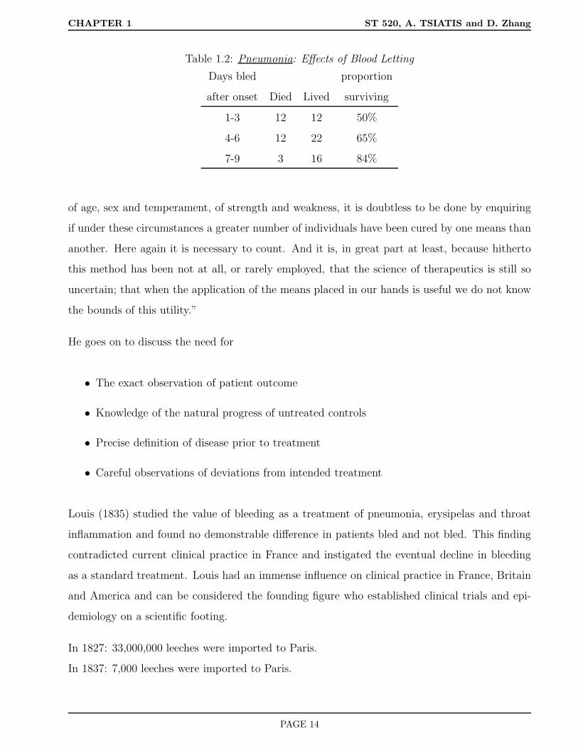
Table 1.2: Pneumonia: Effects of Blood Letting
Days bled proportion
after onset Died Lived surviving
1-3 12 12 50%
4-6 12 22 65%
7-9 3 16 84%
of age, sex and temperament, of strength and weakness, it is doubtless to be done by enquiring
if under these circumstances a greater number of individuals have been cured by one means than
another. Here again it is necessary to count. And it is, in great part at least, because hitherto
this method has been not at all, or rarely employed, that the science of therapeutics is still so
uncertain; that when the application of the means placed in our hands is useful we do not know
the bounds of this utility.”
He goes on to discuss the need for
• The exact observation of patient outcome
• Knowledge of the natural progress of untreated controls
• Precise definition of disease prior to treatment
• Careful observations of deviations from intended treatment
Louis (1835) studied the value of bleeding as a treatment of pneumonia, erysipelas and throat
inflammation and found no demonstrable difference in patients bled and not bled. This finding
contradicted current clinical practice in France and instigated the eventual decline in bleeding
as a standard treatment. Louis had an immense influence on clinical practice in France, Britain
and America and can be considered the founding figure who established clinical trials and epi-
demiology on a scientific footing.
In 1827: 33,000,000 leeches were imported to Paris.
In 1837: 7,000 leeches were imported to Paris.
PAGE 14

CHAPTER 1 ST 520, A. TSIATIS and D. Zhang
Modern clinical trials
The first clinical trial with a properly randomized control group was set up to study streptomycin
in the treatment of pulmonary tuberculosis, sponsored by the Medical Research Council, 1948.
This was a multi-center clinical trial where patients were randomly allocated to streptomycin +
bed rest versus bed rest alone.
The evaluation of patient x-ray films was made independently by two radiologists and a clinician,
each of whom did not know the others evaluations or which treatment the patient was given.
Both patient survival and radiological improvement were significantly better on streptomycin.
The field trial of the Salk Polio Vaccine
In 1954, 1.8 million children participated in the largest trial ever to assess the effectiveness of
the Salk vaccine in preventing paralysis or death from poliomyelitis.
Such a large number was needed because the incidence rate of polio was about 1 per 2,000 and
evidence of treatment effect was needed as soon as possible so that vaccine could be routinely
given if found to be efficacious.
There were two components (randomized and non-randomized) to this trial. For the non-
randomized component, one million children in the first through third grades participated. The
second graders were offered vaccine whereas first and third graders formed the control group.
There was also a randomized component where .8 million children were randomized in a double-
blind placebo-controlled trial.
The incidence of polio in the randomized vaccinated group was less than half that in the control
group and even larger differences were seen in the decline of paralytic polio.
The nonrandomized group supported these results; however non-participation by some who were
offered vaccination might have cast doubt on the results. It turned out that the incidence of polio
among children (second graders) offered vaccine and not taking it (non-compliers) was different
than those in the control group (first and third graders). This may cast doubt whether first and
third graders (control group) have the same likelihood for getting polio as second graders. This is
PAGE 15

CHAPTER 1 ST 520, A. TSIATIS and D. Zhang
a basic assumption that needs to be satisfied in order to make unbiased treatment comparisons.
Luckily, there was a randomized component to the study where the two groups (vaccinated)
versus (control) were guaranteed to be similar on average by design.
Note: During the course of the semester there will be a great deal of discussion on the role of
randomization and compliance and their effect on making causal statements.
Government sponsored studies
In the 1950’s the National Cancer Institute (NCI) organized randomized clinical trials in acute
leukemia. The successful organization of this particular clinical trial led to the formation of two
collaborative groups; CALGB (Cancer and Leukemia Group B) and ECOG (Eastern Cooperative
Oncology Group). More recently SWOG (Southwest Oncology Group) and POG (Pediatrics
Oncology Group) have been organized. A Cooperative group is an organization with many
participating hospitals throughout the country (sometimes world) that agree to conduct common
clinical trials to assess treatments in different disease areas.
Government sponsored clinical trials are now routine. As well as the NCI, these include the
following organizations of the National Institutes of Health.
• NHLBI- (National Heart Lung and Blood Institute) funds individual and often very large
studies in heart disease. To the best of my knowledge there are no cooperative groups
funded by NHLBI.
• NIAID- (National Institute of Allergic and Infectious Diseases) Much of their funding now
goes to clinical trials research for patients with HIV and AIDS. The ACTG (AIDS Clinical
Trials Group) is a large cooperative group funded by NIAID.
• NIDDK- (National Institute of Diabetes and Digestive and Kidney Diseases). Funds large
scale clinical trials in diabetes research. Recently formed the cooperative group TRIALNET
(network 18 clinical centers working in cooperation with screening sites throughout the
United States, Canada, Finland, United Kingdom, Italy, Germany, Australia, and New
Zealand - for type 1 diabetes)
PAGE 16

CHAPTER 1 ST 520, A. TSIATIS and D. Zhang
Pharmaceutical Industry
• Before World War II no formal requirements were made for conducting clinical trials before
a drug could be freely marketed.
• In 1938, animal research was necessary to document toxicity, otherwise human data could
be mostly anecdotal.
• In 1962, it was required that an “adequate and well controlled trial” be conducted.
• In 1969, it became mandatory that evidence from a randomized clinical trial was necessary
to get marketing approval from the Food and Drug Administration (FDA).
• More recently there is effort in standardizing the process of drug approval worldwide. This
has been through efforts of the International Conference on Harmonization (ICH).
website: http://www.pharmweb.net/pwmirror/pw9/ifpma/ich1.html
• There are more clinical trials currently taking place than ever before. The great majority
of the clinical trial effort is supported by the Pharmaceutical Industry for the evaluation
and marketing of new drug treatments. Because the evaluation of drugs and the conduct,
design and analysis of clinical trials depends so heavily on sound Statistical Methodology
this has resulted in an explosion of statisticians working for th Pharmaceutical Industry
and wonderful career opportunities.
PAGE 17
CHAPTER 2 ST 520, A. TSIATIS and D. Zhang
2 Phase I and II clinical trials
2.1 Phases of Clinical Trials
The process of drug development can be broadly classified as pre-clinical and clinical. Pre-
clinical refers to experimentation that occurs before it is given to human subjects; whereas,
clinical refers to experimentation with humans. This course will consider only clinical research.
It will be assumed that the drug has already been developed by the chemist or biologist, tested
in the laboratory for biologic activity (in vitro), that preliminary tests on animals have been
conducted (in vivo) and that the new drug or therapy is found to be sufficiently promising to be
introduced into humans.
Within the realm of clinical research, clinical trials are classified into four phases.
• Phase I: To explore possible toxic effects of drugs and determine a tolerated dose for
further experimentation. Also during Phase I experimentation the pharmacology of the
drug may be explored.
• Phase II: Screening and feasibility by initial assessment for therapeutic effects; further
assessment of toxicities.
• Phase III: Comparison of new intervention (drug or therapy) to the current standard of
treatment; both with respect to efficacy and toxicity.
• Phase IV: (post marketing) Observational study of morbidity/adverse effects.
These definitions of the four phases are not hard and fast. Many clinical trials blur the lines
between the phases. Loosely speaking, the logic behind the four phases is as follows:
A new promising drug is about to be assessed in humans. The effect that this drug might have
on humans is unknown. We might have some experience on similar acting drugs developed in
the past and we may also have some data on the effect this drug has on animals but we are not
sure what the effect is on humans. To study the initial effects, a Phase I study is conducted.
Using increasing doses of the drug on a small number of subjects, the possible side effects of the
drug are documented. It is during this phase that the tolerated dose is determined for future
PAGE 18

CHAPTER 2 ST 520, A. TSIATIS and D. Zhang
experimentation. The general dogma is that the therapeutic effect of the drug will increase with
dose, but also the toxic effects will increase as well. Therefore one of the goals of a Phase I study
is to determine what the maximum dose should be that can be reasonably tolerated by most
individuals with the disease. The determination of this dose is important as this will be used in
future studies when determining the effectiveness of the drug. If we are too conservative then we
may not be giving enough drug to get the full therapeutic effect. On the other hand if we give
too high a dose then people will have adverse effects and not be able to tolerate the drug.
Once it is determined that a new drug can be tolerated and a dose has been established, the
focus turns to whether the drug is good. Before launching into a costly large-scale comparison
of the new drug to the current standard treatment, a smaller feasibility study is conducted to
assess whether there is sufficient efficacy (activity of the drug on disease) to warrant further
investigation. This occurs during phase II where drugs which show little promise are screened
out.
If the new drug still looks promising after phase II investigation it moves to Phase III testing
where a comparison is made to a current standard treatment. These studies are generally large
enough so that important treatment differences can be detected with sufficiently large probability.
These studies are conducted carefully using sound statistical principles of experimental design
established for clinical trials to make objective and unbiased comparisons. It is on the basis of
such Phase III clinical trials that new drugs are approved by regulatory agencies (such as FDA)
for the general population of individuals with the disease for which this drug is targeted.
Once a drug is on the market and a large number of patients are taking it, there is always the
possibility of rare but serious side effects that can only be detected when a large number are
given treatment for sufficiently long periods of time. It is important that a monitoring system
be in place that allows such problems, if they occur, to be identified. This is the role of Phase
IV studies.
A brief discussion of phase I studies and designs and Pharmacology studies will be given based
on the slides from Professor Marie Davidian, an expert in pharmacokinetics. Slides on phase I
and pharmacology will be posted on the course web page.
PAGE 19

CHAPTER 2 ST 520, A. TSIATIS and D. Zhang
2.2 Phase II clinical trials
After a new drug is tested in phase I for safety and tolerability, a dose finding study is sometimes
conducted in phase II to identify a lowest dose level with good efficacy (close to the maximum
efficacy achievable at tolerable dose level). In other situations, a phase II clinical trial uses a
fixed dose chosen on the basis of a phase I clinical trial. The total dose is either fixed or may
vary depending on the weight of the patient. There may also be provisions for modification of
the dose if toxicity occurs. The study population are patients with a specified disease for which
the treatment is targeted.
The primary objective is to determine whether the new treatment should be used in a large-scale
comparative study. Phase II trials are used to assess
• feasibility of treatment
• side effects and toxicity
• logistics of administration and cost
The major issue that is addressed in a phase II clinical trial is whether there is enough evidence
of efficacy to make it worth further study in a larger and more costly clinical trial. In a sense this
is an initial screening tool for efficacy. During phase II experimentation the treatment efficacy
is often evaluated on surrogate markers; i.e on an outcome that can be measured quickly and
is believed to be related to the clinical outcome.
Example: Suppose a new drug is developed for patients with lung cancer. Ultimately, we
would like to know whether this drug will extend the life of lung cancer patients as compared to
currently available treatments. Establishing the effect of a new drug on survival would require a
long study with relatively large number of patients and thus may not be suitable as a screening
mechanism. Instead, during phase II, the effect of the new drug may be assessed based on tumor
shrinkage in the first few weeks of treatment. If the new drug shrinks tumors sufficiently for a
sufficiently large proportion of patients, then this may be used as evidence for further testing.
In this example, tumor shrinkage is a surrogate marker for overall survival time. The belief is
that if the drug has no effect on tumor shrinkage it is unlikely to have an effect on the patient’s
PAGE 20

CHAPTER 2 ST 520, A. TSIATIS and D. Zhang
overall survival and hence should be eliminated from further consideration. Unfortunately, there
are many instances where a drug has a short term effect on a surrogate endpoint but ultimately
may not have the long term effect on the clinical endpoint of ultimate interest. Furthermore,
sometimes a drug may have beneficial effect through a biological mechanism that is not detected
by the surrogate endpoint. Nonetheless, there must be some attempt at limiting the number of
drugs that will be considered for further testing or else the system would be overwhelmed.
Other examples of surrogate markers are
• Lowering blood pressure or cholesterol for patients with heart disease
• Increasing CD4 counts or decreasing viral load for patients with HIV disease
Most often, phase II clinical trials do not employ formal comparative designs. That is, they do
not use parallel treatment groups. Often, phase II designs employ more than one stage; i.e. one
group of patients are given treatment; if no (or little) evidence of efficacy is observed, then the
trial is stopped and the drug is declared a failure; otherwise, more patients are entered in the
next stage after which a final decision is made whether to move the drug forward or not.
2.2.1 Statistical Issues and Methods
One goal of a phase II trial is to estimate an endpoint related to treatment efficacy with sufficient
precision to aid the investigators in determining whether the proposed treatment should be
studied further.
Some examples of endpoints are:
• proportion of patients responding to treatment (response has to be unambiguously defined)
• proportion with side effects
• average decrease in blood pressure over a two week period
A statistical perspective is generally taken for estimation and assessment of precision. That
is, the problem is often posed through a statistical model with population parameters to be
estimated and confidence intervals for these parameters to assess precision.
PAGE 21

CHAPTER 2 ST 520, A. TSIATIS and D. Zhang
Example: Suppose we consider patients with esophogeal cancer treated with chemotherapy prior
to surgical resection. A complete response is defined as an absence of macroscopic or microscopic
tumor at the time of surgery. We suspect that this may occur with 35% (guess) probability using
a drug under investigation in a phase II study. The 35% is just a guess, possibly based on similar
acting drugs used in the past, and the goal is to estimate the actual response rate with sufficient
precision, in this case we want the 95% confidence interval to be within 15% of the truth.
As statisticians, we view the world as follows: We start by positing a statistical model; that is,
let π denote the population complete response rate. We conduct an experiment: n patients with
esophogeal cancer are treated with the chemotherapy prior to surgical resection and we collect
data: the number of patients who have a complete response.
The result of this experiment yields a random variable X, the number of patients in a sample of
size n that have a complete response. A popular model for this scenario is to assume that
X ∼ binomial(n, π);
that is, the random variable X is distributed with a binomial distribution with sample size n and
success probability π. The goal of the study is to estimate π and obtain a confidence interval.
I believe it is worth stepping back a little and discussing how the actual experiment and the
statistical model used to represent this experiment relate to each other and whether the implicit
assumptions underlying this relationship are reasonable.
Statistical Model
What is the population? All people now and in the future with esophogeal cancer who would
be eligible for the treatment.
What is π? (the population parameter)
If all the people in the hypothetical population above were given the new chemotherapy, then π
would be the proportion who would have a complete response. This is a hypothetical construct.
Neither can we identify the population above or could we actually give them all the chemotherapy.
Nonetheless, let us continue with this mind experiment.
PAGE 22

CHAPTER 2 ST 520, A. TSIATIS and D. Zhang
We assume the random variable X follows a binomial distribution. Is this reasonable? Let us
review what it means for a random variable to follow a binomial distribution.
X being distributed as a binomial b(n, π) means that X corresponds to the number of successes
(complete responses) in n independent trials where the probability of success for each trial is
equal to π. This would be satisfied, for example, if we were able to identify every member of the
population and then, using a random number generator, chose n individuals at random from our
population to test and determine the number of complete responses.
Clearly, this is not the case. First of all, the population is a hypothetical construct. Moreover,
in most clinical studies the sample that is chosen is an opportunistic sample. There is gen-
erally no attempt to randomly sample from a specific population as may be done in a survey
sample. Nonetheless, a statistical perspective may be a useful construct for assessing variability.
I sometimes resolve this in my own mind by thinking of the hypothetical population that I can
make inference on as all individuals who might have been chosen to participate in the study
with whatever process that was actually used to obtain the patients that were actually studied.
However, this limitation must always be kept in mind when one extrapolates the results of a
clinical experiment to a more general population.
Philosophical issues aside, let us continue by assuming that the posited model is a reasonable
approximation to some question of relevance. Thus, we will assume that our data is a realization
of the random variable X, assumed to be distributed as b(n, π), where π is the population
parameter of interest.
Reviewing properties about a binomial distribution we note the following:
• E(X) = nπ, where E(·) denotes expectation of the random variable.
• V ar(X) = nπ(1 − π), where V ar(·) denotes the variance of the random variable.
• P (X = k) =
n
k
πk(1−π)n−k, where P (·) denotes probability of an event, and
n
k
=
n!k!(n−k)!
• Denote the sample proportion by p = X/n, then
– E(p) = π
PAGE 23
CHAPTER 2 ST 520, A. TSIATIS and D. Zhang
– V ar(p) = π(1 − π)/n
• When n is sufficiently large, the distribution of the sample proportion p = X/n is well
approximated by a normal distribution with mean π and variance π(1 − π)/n:
p ∼ N(π, π(1 − π)/n).
This approximation is useful for inference regarding the population parameter π. Because of the
approximate normality, the estimator p will be within 1.96 standard deviations of π approxi-
mately 95% of the time. (Approximation gets better with increasing sample size). Therefore the
population parameter π will be within the interval
p± 1.96π(1 − π)/n1/2
with approximately 95% probability. Since the value π is unknown to us, we approximate using
p to obtain the approximate 95% confidence interval for π, namely
p± 1.96p(1 − p)/n1/2.
Going back to our example, where our best guess for the response rate is about 35%, if we want
the precision of our estimator to be such that the 95% confidence interval is within 15% of the
true π, then we need
1.96(.35)(.65)
n1/2 = .15,
or
n =(1.96)2(.35)(.65)
(.15)2= 39 patients.
Since the response rate of 35% is just a guess which is made before data are collected, the exercise
above should be repeated for different feasible values of π before finally deciding on how large
the sample size should be.
Exact Confidence Intervals
If either nπ or n(1−π) is small, then the normal approximation given above may not be adequate
for computing accurate confidence intervals. In such cases we can construct exact (usually
conservative) confidence intervals.
PAGE 24
CHAPTER 2 ST 520, A. TSIATIS and D. Zhang
We start by reviewing the definition of a confidence interval and then show how to construct an
exact confidence interval for the parameter π of a binomial distribution.
Definition: The definition of a (1− α)-th confidence region (interval) for the parameter π is as
follows:
For each realization of the data X = k, a region of the parameter space, denoted by C(k) (usually
an interval) is defined in such a way that the random region C(X) contains the true value of
the parameter with probability greater than or equal to (1 − α) regardless of the value of the
parameter. That is,
PπC(X) ⊃ π ≥ 1 − α, for all 0 ≤ π ≤ 1,
where Pπ(·) denotes probability calculated under the assumption that X ∼ b(n, π) and ⊃ denotes
“contains”. The confidence interval is the random interval C(X). After we collect data and obtain
the realization X = k, then the corresponding confidence interval is defined as C(k).
This definition is equivalent to defining an acceptance region (of the sample space) for each value
π, denoted as A(π), that has probability greater than equal to 1− α, i.e.
PπX ∈ A(π) ≥ 1 − α, for all 0 ≤ π ≤ 1,
in which case C(k) = π : k ∈ A(π).
We find it useful to consider a graphical representation of the relationship between confidence
intervals and acceptance regions.
PAGE 25
CHAPTER 2 ST 520, A. TSIATIS and D. Zhang
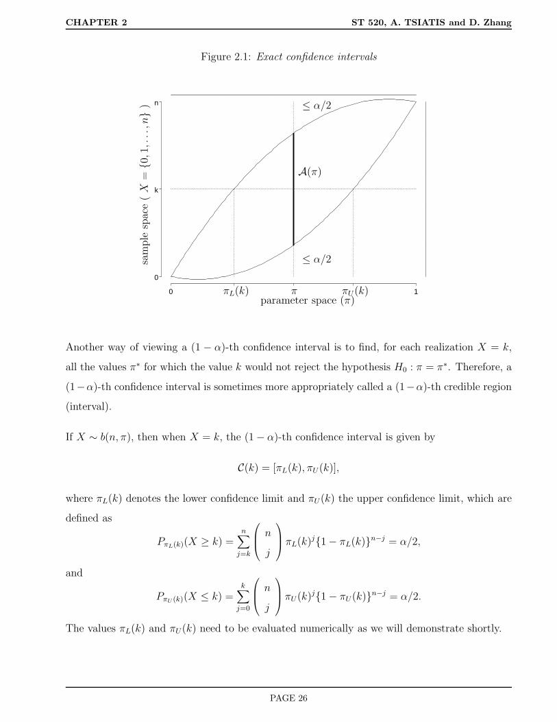
Figure 2.1: Exact confidence intervals
0 1
0
k
n
sam
ple
spac
e(X
=0,1,...,n
) ≤ α/2
≤ α/2
A(π)
πL(k) πU(k)parameter space (π)
π
Another way of viewing a (1 − α)-th confidence interval is to find, for each realization X = k,
all the values π∗ for which the value k would not reject the hypothesis H0 : π = π∗. Therefore, a
(1−α)-th confidence interval is sometimes more appropriately called a (1−α)-th credible region
(interval).
If X ∼ b(n, π), then when X = k, the (1 − α)-th confidence interval is given by
C(k) = [πL(k), πU(k)],
where πL(k) denotes the lower confidence limit and πU(k) the upper confidence limit, which are
defined as
PπL(k)(X ≥ k) =n∑
j=k
n
j
πL(k)j1 − πL(k)n−j = α/2,
and
PπU (k)(X ≤ k) =k∑
j=0
n
j
πU(k)j1 − πU(k)n−j = α/2.
The values πL(k) and πU(k) need to be evaluated numerically as we will demonstrate shortly.
PAGE 26

CHAPTER 2 ST 520, A. TSIATIS and D. Zhang
Remark: Since X has a discrete distribution, the way we define the (1−α)-th confidence interval
above will yield
PπC(X) ⊃ π > 1 − α
(strict inequality) for most values of 0 ≤ π ≤ 1. Strict equality cannot be achieved because of
the discreteness of the binomial random variable.
Example: In a Phase II clinical trial, 3 of 19 patients respond to α-interferon treatment for
multiple sclerosis. In order to find the exact confidence 95% interval for π for X = k, k = 3, and
n = 19, we need to find πL(3) and πU (3) satisfying
PπL(3)(X ≥ 3) = .025; PπU (3)(X ≤ 3) = .025.
Many textbooks have tables for P (X ≤ c), where X ∼ b(n, π) for some n’s and π’s. Alternatively,
P (X ≤ c) can be obtained using statistical software such as SAS or R. Either way, we see that
πU(3) ≈ .40. To find πL(3) we note that
PπL(3)(X ≥ 3) = 1 − PπL(3)(X ≤ 2).
Consequently, we must search for πL(3) such that
PπL(3)(X ≤ 2) = .975.
This yields πL(3) ≈ .03. Hence the “exact” 95% confidence interval for π is
[.03, .40].
In contrast, the normal approximation yields a confidence interval of
3
19± 1.96
(319
× 1619
19
)1/2
= [−.006, .322].
PAGE 27

CHAPTER 2 ST 520, A. TSIATIS and D. Zhang
2.2.2 Gehan’s Two-Stage Design
Discarding ineffective treatments early
If it is unlikely that a treatment will achieve some minimal level of response or efficacy, we may
want to stop the trial as early as possible. For example, suppose that a 20% response rate is the
lowest response rate that is considered acceptable for a new treatment. If we get no responses in
n patients, with n sufficiently large, then we may feel confident that the treatment is ineffective.
Statistically, this may be posed as follows: How large must n be so that if there are 0 responses
among n patients we are relatively confident that the response rate is not 20% or better? If
X ∼ b(n, π), and if π ≥ .2, then
Pπ(X = 0) = (1 − π)n ≤ (1 − .2)n = .8n.
Choose n so that .8n = .05 or n ln(8) = ln(.05). This leads to n ≈ 14 (rounding up). Thus, with
14 patients, it is unlikely (≤ .05) that no one would respond if the true response rate was greater
than 20%. Thus 0 patients responding among 14 might be used as evidence to stop the phase II
trial and declare the treatment a failure.
This is the logic behind Gehan’s two-stage design. Gehan suggested the following strategy: If
the minimal acceptable response rate is π0, then choose the first stage with n0 patients such that
(1 − π0)n0 = .05; n0 =
ln(.05)
ln(1 − π0);
if there are 0 responses among the first n0 patients then stop and declare the treatment a failure;
otherwise, continue with additional patients that will ensure a certain degree of predetermined
accuracy in the 95% confidence interval.
If, for example, we wanted the 95% confidence interval for the response rate to be within ±15%
when a treatment is considered minimally effective at π0 = 20%, then the sample size necessary
for this degree of precision is
1.96(.2 × .8
n
)1/2
= .15, or n = 28.
In this example, Gehan’s design would treat 14 patients initially. If none responded, the treatment
would be declared a failure and the study stopped. If there was at least one response, then another
14 patients would be treated and a 95% confidence interval for π would be computed using the
data from all 28 patients.
PAGE 28

CHAPTER 2 ST 520, A. TSIATIS and D. Zhang
2.2.3 Simon’s Two-Stage Design
Another way of using two-stage designs was proposed by Richard Simon. Here, the investigators
must decide on values π0, and π1, with π0 < π1 for the probability of response so that
• If π ≤ π0, then we want to declare the drug ineffective with high probability, say 1 − α,
where α is taken to be small.
• If π ≥ π1, then we want to consider this drug for further investigation with high probability,
say 1 − β, where β is taken to be small.
The values of α and β are generally taken to be between .05 and .20.
The region of the parameter space π0 < π < π1 is the indifference region.
0 1
Drug is ineffective Indifference region Drug is effective
π0 π1
π = response rate
A two-stage design would proceed as follows: Integers n1, n, r1, r, with n1 < n, r1 < n1, and
r < n are chosen (to be described later) and
• n1 patients are given treatment in the first stage. If r1 or less respond, then declare the
treatment a failure and stop.
• If more than r1 respond, then add (n− n1) additional patients for a total of n patients.
• At the second stage, if the total number that respond among all n patients is greater than
r, then declare the treatment a success; otherwise, declare it a failure.
PAGE 29

CHAPTER 2 ST 520, A. TSIATIS and D. Zhang
Statistically, this decision rule is the following: Let X1 denote the number of responses in the
first stage (among the n1 patients) and X2 the number of responses in the second stage (among
the n− n1 patients). X1 and X2 are assumed to be independent binomially distributed random
variables, X1 ∼ b(n1, π) and X2 ∼ b(n2, π), where n2 = n− n1 and π denotes the probability of
response. Declare the treatment a failure if
(X1 ≤ r1) or (X1 > r1) and (X1 +X2 ≤ r),
otherwise, the treatment is declared a success if
(X1 > r1) and (X1 +X2) > r).
Note: If n1 > r and if the number of patients responding in the first stage is greater than r,
then there is no need to proceed to the second stage to declare the treatment a success.
According to the constraints of the problem we want
P (declaring treatment success|π ≤ π0) ≤ α,
or equivalently
P(X1 > r1) and (X1 +X2 > r)|π = π0 ≤ α︸ ︷︷ ︸; (2.1)
Note: If the above inequality is true when π = π0, then it is true when π < π0.
Also, we want
P (declaring treatment failure|π ≥ π1) ≤ β,
or equivalently
P(X1 > r1) and (X1 +X2 > r)|π = π1 ≥ 1 − β. (2.2)
Question: How are probabilities such as P(X1 > r1) and (X1 +X2 > r)|π computed?
Since X1 and X2 are independent binomial random variables, then for any integer 0 ≤ m1 ≤ n1
and integer 0 ≤ m2 ≤ n2, the
P (X1 = m1, X2 = m2|π) = P (X1 = m1|π) × P (X2 = m2|π)
=
n1
m1
πm1(1 − π)n1−m1
n2
m2
πm2(1 − π)n2−m2
.
PAGE 30

CHAPTER 2 ST 520, A. TSIATIS and D. Zhang
We then have to identify the pairs (m1, m2) where (m1 > r1) and (m1 + m2) > r, find the
probability for each such (m1, m2) pair using the equation above, and then add all the appropriate
probabilities.
We illustrate this in the following figure:
Figure 2.2: Example: n1 = 8, n = 14, X1 > 3, and X1 +X2 > 6
0 2 4 6 8
01
23
45
6
X1
X2
As it turns out there are many combinations of (r1, n1, r, n) that satisfy the constraints (2.1) and
(2.2) for specified (π0, π1, α, β). Through a computer search one can find the “optimal design”
among these possibilities, where the optimal design is defined as the combination (r1, n1, r, n),
satisfying the constraints (2.1) and (2.2), which gives the smallest expected sample size when
PAGE 31

CHAPTER 2 ST 520, A. TSIATIS and D. Zhang
π = π0.
The expected sample size for a two stage design is defined as
n1P (stopping at the first stage) + nP (stopping at the second stage).
For our problem, the expected sample size is given by
n1P (X1 ≤ r1|π = π0) + P (X1 > r|π = π0) + nP (r1 + 1 ≤ X1 ≤ r|π = π0).
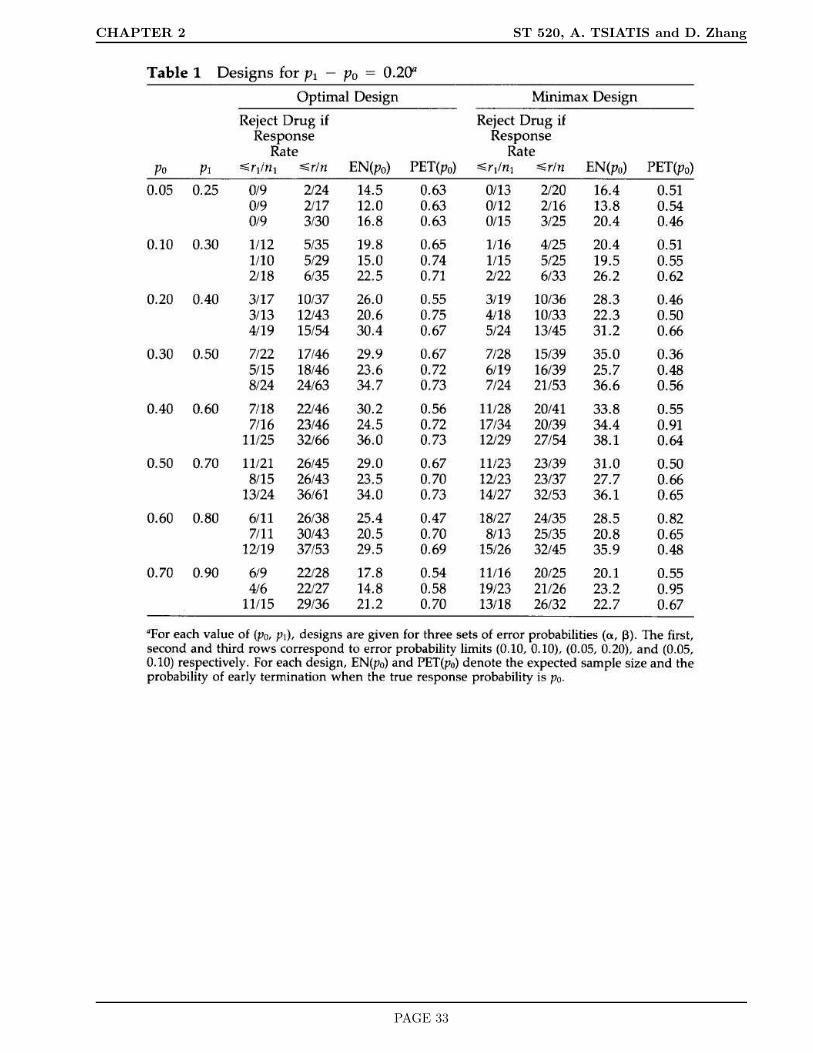
Optimal two-stage designs have been tabulated for a variety of (π0, π1, α, β) in the article
Simon, R. (1989). Optimal two-stage designs for Phase II clinical trials. Controlled Clinical
Trials. 10: 1-10.
The tables are given on the next two pages.
PAGE 32
CHAPTER 2 ST 520, A. TSIATIS and D. Zhang
PAGE 33

CHAPTER 2 ST 520, A. TSIATIS and D. Zhang
PAGE 34
CHAPTER 3 ST 520, A. TSIATIS and D. Zhang
3 Phase III Clinical Trials
3.1 Why are clinical trials needed
A clinical trial is the clearest method of determining whether an intervention has the postulated
effect. It is very easy for anecdotal information about the benefit of a therapy to be accepted
and become standard of care. The consequence of not conducting appropriate clinical trials can
be serious and costly. As we discussed earlier, because of anecdotal information, blood-letting
was common practice for a very long time. Other examples include
• It was believed that high concentrations of oxygen was useful for therapy in premature
infants until a clinical trial demonstrated its harm
• Intermittent positive pressure breathing became an established therapy for chronic obstruc-
tive pulmonary disease (COPD). Much later, a clinical trial suggested no major benefit for
this very expensive procedure
• Laetrile (a drug extracted from grapefruit seeds) was rumored to be the wonder drug
for Cancer patients even though there was no scientific evidence that this drug had any
biological activity. People were so convinced that there was a conspiracy by the medical
profession to withhold this drug that they would get it illegally from “quacks” or go to
other countries such as Mexico to get treatment. The use of this drug became so prevalent
that the National Institutes of Health finally conducted a clinical trial where they proved
once and for all that Laetrile had no effect. You no longer hear about this issue any more.
• The Cardiac Antiarhythmia Suppression Trial (CAST) documented that commonly used
antiarhythmia drugs were harmful in patients with myocardial infarction
• More recently, against common belief, it was shown that prolonged use of Hormone Re-
placement Therapy for women following menopause may have deleterious effects.
PAGE 35

CHAPTER 3 ST 520, A. TSIATIS and D. Zhang
3.2 Issues to consider before designing a clinical trial
David Sackett gives the following six prerequisites
1. The trial needs to be done
(i) the disease must have either high incidence and/or serious course and poor prognosis
(ii) existing treatment must be unavailable or somehow lacking
(iii) The intervention must have promise of efficacy (pre-clinical as well as phase I-II evi-
dence)
2. The trial question posed must be appropriate and unambiguous
3. The trial architecture is valid. Random allocation is one of the best ways that treatment
comparisons made in the trial are valid. Other methods such as blinding and placebos
should be considered when appropriate
4. The inclusion/exclusion criteria should strike a balance between efficiency and generaliz-
ibility. Entering patients at high risk who are believed to have the best chance of response
will result in an efficient study. This subset may however represent only a small segment
of the population of individuals with disease that the treatment is intended for and thus
reduce the study’s generalizibility
5. The trial protocol is feasible
(i) The protocol must be attractive to potential investigators
(ii) Appropriate types and numbers of patients must be available
6. The trial administration is effective.
Other issues that also need to be considered
• Applicability: Is the intervention likely to be implemented in practice?
• Expected size of effect: Is the intervention “strong enough” to have a good chance of
producing a detectable effect?
PAGE 36

CHAPTER 3 ST 520, A. TSIATIS and D. Zhang
• Obsolescence: Will changes in patient management render the results of a trial obsolete
before they are available?
Objectives and Outcome Assessment
• Primary objective: What is the primary question to be answered?
– ideally just one
– important, relevant to care of future patients
– capable of being answered
• Primary outcome (endpoint)
– ideally just one
– relatively simple to analyze and report
– should be well defined; objective measurement is preferred to a subjective one. For
example, clinical and laboratory measurements are more objective than say clinical
and patient impression
• Secondary Questions
– other outcomes or endpoints of interest
– subgroup analyses
– secondary questions should be viewed as exploratory
∗ trial may lack power to address them
∗ multiple comparisons will increase the chance of finding “statistically significant”
differences even if there is no effect
– avoid excessive evaluations; as well as problem with multiple comparisons, this may
effect data quality and patient support
PAGE 37
CHAPTER 3 ST 520, A. TSIATIS and D. Zhang
Choice of Primary Endpoint
Example: Suppose we are considering a study to compare various treatments for patients with
HIV disease, then what might be the appropriate primary endpoint for such a study? Let us
look at some options and discuss them.
The HIV virus destroys the immune system; thus individuals infected are susceptible to various
opportunistic infections which ultimately leads to death. Many of the current treatments are
designed to target the virus either trying to destroy it or, at least, slow down its replication.
Other treatments may target specific opportunistic infections.
Suppose we have a treatment intended to attack the virus directly, Here are some possibilities
for the primary endpoint that we may consider.
1. Increase in CD4 count. Since CD4 count is a direct measure of the immune function and
CD4 cells are destroyed by the virus, we might expect that a good treatment will increase
CD4 count.
2. Viral RNA reduction. Measures the amount of virus in the body
3. Time to the first opportunistic infection
4. Time to death from any cause
5. Time to death or first opportunistic infection, whichever comes first
Outcomes 1 and 2 may be appropriate as the primary outcome in a phase II trial where we want
to measure the activity of the treatment as quickly as possible.
Outcome 4 may be of ultimate interest in a phase III trial, but may not be practical for studies
where patients have a long expected survival and new treatments are being introduced all the
time. (Obsolescence)
Outcome 5 may be the most appropriate endpoint in a phase III trial. However, the other
outcomes may be reasonable for secondary analyses.
PAGE 38

CHAPTER 3 ST 520, A. TSIATIS and D. Zhang
3.3 Ethical Issues
A clinical trial involves human subjects. As such, we must be aware of ethical issues in the design
and conduct of such experiments. Some ethical issues that need to be considered include the
following:
• No alternative which is superior to any trial intervention is available for each subject
• Equipoise–There should be genuine uncertainty about which trial intervention may be
superior for each individual subject before a physician is willing to allow their patients to
participate in such a trial
• Exclude patients for whom risk/benefit ratio is likely to be unfavorable
– pregnant women if possibility of harmful effect to the fetus
– too sick to benefit
– if prognosis is good without interventions
Justice Considerations
• Should not exclude a class of patients for non medical reasons nor unfairly recruit patients
from poorer or less educated groups
This last issue is a bit tricky as “equal access” may hamper the evaluation of interventions. For
example
• Elderly people may die from diseases other than that being studied
• IV drug users are more difficult to follow in AIDS clinical trials
PAGE 39

CHAPTER 3 ST 520, A. TSIATIS and D. Zhang
3.4 The Randomized Clinical Trial
The objective of a clinical trial is to evaluate the effects of an intervention. Evaluation implies
that there must be some comparison either to
• no intervention
• placebo
• best therapy available
Fundamental Principle in Comparing Treatment Groups
Groups must be alike in all important aspects and only differ in the treatment which each group
receives. Otherwise, differences in response between the groups may not be due to the treatments
under study, but can be attributed to the particular characteristics of the groups.
How should the control group be chosen
Here are some examples:
• Literature controls
• Historical controls
• Patient as his/her own control (cross-over design)
• Concurrent control (non-randomized)
• Randomized concurrent control
The difficulty in non-randomized clinical trials is that the control group may be different prog-
nostically from the intervention group. Therefore, comparisons between the intervention and
control groups may be biased. That is, differences between the two groups may be due to factors
other than the treatment.
PAGE 40
CHAPTER 3 ST 520, A. TSIATIS and D. Zhang
Attempts to correct the bias that may be induced by these confounding factors either by design
(matching) or by analysis (adjustment through stratified analysis or regression analysis) may not
be satisfactory.
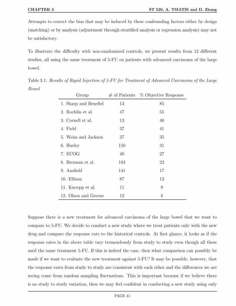
To illustrate the difficulty with non-randomized controls, we present results from 12 different
studies, all using the same treatment of 5-FU on patients with advanced carcinoma of the large
bowel.
Table 3.1: Results of Rapid Injection of 5-FU for Treatment of Advanced Carcinoma of the Large
Bowel
Group # of Patients % Objective Response
1. Sharp and Benefiel 13 85
2. Rochlin et al. 47 55
3. Cornell et al. 13 46
4. Field 37 41
5. Weiss and Jackson 37 35
6. Hurley 150 31
7. ECOG 48 27
8. Brennan et al. 183 23
9. Ansfield 141 17
10. Ellison 87 12
11. Knoepp et al. 11 9
12. Olson and Greene 12 8
Suppose there is a new treatment for advanced carcinoma of the large bowel that we want to
compare to 5-FU. We decide to conduct a new study where we treat patients only with the new
drug and compare the response rate to the historical controls. At first glance, it looks as if the
response rates in the above table vary tremendously from study to study even though all these
used the same treatment 5-FU. If this is indeed the case, then what comparison can possibly be
made if we want to evaluate the new treatment against 5-FU? It may be possible, however, that
the response rates from study to study are consistent with each other and the differences we are
seeing come from random sampling fluctuations. This is important because if we believe there
is no study to study variation, then we may feel confident in conducting a new study using only
PAGE 41

CHAPTER 3 ST 520, A. TSIATIS and D. Zhang
the new treatment and comparing the response rate to the pooled response rate from the studies
above. How can we assess whether these differences are random sampling fluctuations or real
study to study differences?
Hierarchical Models
To address the question of whether the results from the different studies are random samples
from underlying groups with a common response rate or from groups with different underlying
response rates, we introduce the notion of a hierarchical model. In a hierarchical model, we
assume that each of the N studies that were conducted were from possibly N different study
groups each of which have possibly different underlying response rates π1, . . . , πN . In a sense, we
now think of the world as being made of many different study groups (or a population of study
groups), each with its own response rate, and that the studies that were conducted correspond
to choosing a small sample of these population study groups. As such, we imagine π1, . . . , πN to
be a random sample of study-specific response rates from a larger population of study groups.
Since πi, the response rate from the i-th study group, is a random variable, it has a mean and
and a variance which we will denote by µπ and σ2π. Since we are imagining a super-population
of study groups, each with its own response rate, that we are sampling from, we conceptualize
µπ and σ2π to be the average and variance of these response rates from this super-population.
Thus π1, . . . , πN will correspond to an iid (independent and identically distributed) sample from
a population with mean µπ and variance σ2π. I.e.
π1, . . . , πN , are iid with E(πi) = µπ, var(πi) = σ2π, i = 1, . . . , N.
This is the first level of the hierarchy.
The second level of the hierarchy corresponds now to envisioning that the data collected from
the i-th study (ni, Xi), where ni is the number of patients treated in the i-th study and Xi is
the number of complete responses among the ni treated, is itself a random sample from the i-th
study group whose response rate is πi. That is, conditional on ni and πi, Xi is assumed to follow
a binomial distribution, which we denote as
Xi|ni, πi ∼ b(ni, πi).
This hierarchical model now allows us to distinguish between random sampling fluctuation and
real study to study differences. If all the different study groups were homogeneous, then there
PAGE 42

CHAPTER 3 ST 520, A. TSIATIS and D. Zhang
should be no study to study variation, in which case σ2π = 0. Thus we can evaluate the degree
of study to study differences by estimating the parameter σ2π.
In order to obtain estimates for σ2π, we shall use some classical results of conditional expectation
and conditional variance. Namely, if X and Y denote random variables for some probability
experiment then the following is true
E(X) = EE(X|Y )
and
var(X) = Evar(X|Y ) + varE(X|Y ).
Although these results are known to many of you in the class; for completeness, I will sketch out
the arguments why the two equalities above are true.
3.5 Review of Conditional Expectation and Conditional Variance
For simplicity, I will limit myself to probability experiments with a finite number of outcomes.
For random variables that are continuous one needs more complicated measure theory for a
rigorous treatment.
Probability Experiment
Denote the result of an experiment by one of the outcomes in the sample space Ω = ω1, . . . , ωk.For example, if the experiment is to choose one person at random from a population of sizeN with
a particular disease, then the result of the experiment is Ω = A1, . . . , AN where the different A’s
uniquely identify the individuals in the population, If the experiment were to sample n individuals
from the population then the outcomes would be all possible n-tuple combinations of these N
individuals; for example Ω = (Ai1, . . . , Ain), for all i1, . . . , in = 1, . . . , N . With replacement
there are k = Nnth combinations; without replacement there are k = N×(N−1)×. . .×(N−n+1)
combinations of outcomes if order of subjects in the sample is important, and k =
N
n
combinations of outcomes if order is not important.
Denote by p(ω) the probability of outcome ω occurring, where∑
ω∈Ω p(ω) = 1.
PAGE 43
CHAPTER 3 ST 520, A. TSIATIS and D. Zhang
Random variable
A random variable, usually denoted by a capital Roman letter such as X, Y, . . . is a function that
assigns a number to each outcome in the sample space. For example, in the experiment where
we sample one individual from the population
X(ω)= survival time for person ω
Y (ω)= blood pressure for person ω
Z(ω)= height of person ω
The probability distribution of a random variable X is just a list of all different possible
values that X can take together with the corresponding probabilities.
i.e. (x, P (X = x)), for all possible x, where P (X = x) =∑
ω:X(ω)=x p(ω).
The mean or expectation of X is
E(X) =∑
ω∈Ω
X(ω)p(ω) =∑
x
xP (X = x),
and the variance of X is
var(X) =∑
ω∈Ω
X(ω) −E(X)2p(ω) =∑
x
x−E(X)2P (X = x)
= EX − E(X)2 = E(X2) − E(X)2.
Conditional Expectation
Suppose we have two random variablesX and Y defined for the same probability experiment, then
we denote the conditional expectation of X, conditional on knowing that Y = y, by E(X|Y = y)
and this is computed as
E(X|Y = y) =∑
ω:Y (ω)=y
X(ω)p(ω)
P (Y = y).
The conditional expectation of X given Y , denoted by E(X|Y ) is itself a random variable which
assigns the value E(X|Y = y) to every outcome ω for which Y (ω) = y. Specifically, we note
that E(X|Y ) is a function of Y .
PAGE 44

CHAPTER 3 ST 520, A. TSIATIS and D. Zhang
Since E(X|Y ) is itself a random variable, it also has an expectation given by EE(X|Y ). By
the definition of expectation this equals
EE(X|Y ) =∑
ω∈Ω
E(X|Y )(ω)p(ω).
By rearranging this sum, first within the partition ω : Y (ω) = y, and then across the partitions
for different values of y, we get
EE(X|Y ) =∑
y
∑ω:Y (ω)=y X(ω)p(ω)
P (Y = y)
P (Y = y)
=∑
ω∈Ω
X(ω)p(ω) = E(X).
Thus we have proved the very important result that
EE(X|Y ) = E(X).
Conditional Variance
There is also a very important relationship involving conditional variance. Just like conditional
expectation. the conditional variance of X given Y , denoted as var(X|Y ), is a random variable,
which assigns the value var(X|Y = y) to each outcome ω, where Y (ω) = y, and
var(X|Y = y) = E[X −E(X|Y = y)2|Y = y] =∑
ω:Y (ω)=y
X(ω) −E(X|Y = y)2 p(ω)
p(Y = y).
Equivalently,
var(X|Y = y) = E(X2|Y = y) − E(X|Y = y)2.
It turns out that the variance of a random variable X equals
var(X) = Evar(X|Y ) + varE(X|Y ).
This follows because
Evar(X|Y ) = E[E(X2|Y ) − E(X|Y )2] = E(X2) − E[E(X|Y )2] (3.1)
and
varE(X|Y ) = E[E(X|Y )2] − [EE(X|Y )]2 = E[E(X|Y )2] − E(X)2 (3.2)
PAGE 45

CHAPTER 3 ST 520, A. TSIATIS and D. Zhang
Adding (3.1) and (3.2) together yields
Evar(X|Y ) + varE(X|Y ) = E(X2) − E(X)2 = var(X),
as desired.
If we think of partitioning the sample space into regions ω : Y (ω) = y for different values of
y, then the formula above can be interpreted in words as
“the variance of X is equal to the mean of the within partition variances of X plus the variance
of the within partition means of X”. This kind of partitioning of variances is often carried out
in ANOVA models.
Return to Hierarchical Models
Recall
Xi|ni, πi ∼ b(ni, πi), i = 1, . . . , N
and
π1, . . . , πN are iid (µπ, σ2π).
Let pi = Xi/ni denote the sample proportion that respond from the i-th study. We know from
properties of a binomial distribution that
E(pi|πi, ni) = πi
and
var(pi|πi, ni) =πi(1 − πi)
ni.
Note: In our conceptualization of this problem the probability experiment consists of
1. Conducting N studies from a population of studies
2. For each study i we sample ni individuals at random from the i-th study group and count
the number of responses Xi
3. Let us also assume that the sample sizes n1, . . . , nN are random variables from some dis-
tribution.
PAGE 46

CHAPTER 3 ST 520, A. TSIATIS and D. Zhang
4. The results of this experiment can be summarized by the iid random vectors
(πi, ni, Xi), i = 1, . . . , N.
In actuality, we don’t get to see the values πi, i = 1, . . . , N . They are implicitly defined, yet very
important in the description of the model. Often, the values πi are referred to as random effects.
Thus, the observable data we get to work with are
(ni, Xi), i = 1, . . . , N.
Using the laws of iterated conditional expectation and variance just derived, we get the following
results:
E(pi) = EE(pi|ni, πi) = E(πi) = µπ, (3.3)
var(pi) = Evar(pi|ni, πi) + varE(pi|ni, πi)
= E
πi(1 − πi)
ni
+ var(πi)
= E
πi(1 − πi)
ni
+ σ2
π. (3.4)
Since the random variables pi, i = 1, . . . , N are iid, an unbiased estimator for E(pi) = µπ is
given by the sample mean
p = N−1N∑
i=1
pi,
and an unbiased estimator of the variance var(pi) is the sample variance
s2p =
∑Ni=1(pi − p)2
N − 1.
One can also show, using properties of a binomial distribution, that a conditionally unbiased
estimator for πi(1−πi)ni
, conditional on ni and πi, is given by pi(1−pi)ni−1
; that is
E
pi(1 − pi)
ni − 1|ni, πi
=πi(1 − πi)
ni
.
I will leave this as a homework exercise for you to prove.
Since pi(1−pi)ni−1
, i = 1, N are iid random variables with mean
E
pi(1 − pi)
ni − 1
= E
[E
pi(1 − pi)
ni − 1|ni, πi
]
PAGE 47

CHAPTER 3 ST 520, A. TSIATIS and D. Zhang
= E
πi(1 − πi)
ni
,
this means that we can obtain an unbiased estimator for E
πi(1−πi)ni
by using
N−1N∑
i=1
pi(1 − pi)
ni − 1.
Summarizing these results, we have shown that
• s2p =
∑N
i=1(pi−p)2
N−1is an unbiased estimator for var(pi) which by (3.4) equals
E
πi(1 − πi)
ni
+ σ2
π
• We have also shown that N−1∑Ni=1
pi(1−pi)ni−1
is an unbiased estimator for
E
πi(1 − πi)
ni
Consequently, by subtraction, we get that the estimator
σ2π =
∑Ni=1(pi − p)2
N − 1
−N−1
N∑
i=1
pi(1 − pi)
ni − 1
is an unbiased estimator for σ2π.
Going back to the example given in Table 3.1, we obtain the following:
• ∑Ni=1(pi − p)2
N − 1= .0496
•N−1
N∑
i=1
pi(1 − pi)
ni − 1= .0061
• Hence
σ2π = .0496 − .0061 = .0435
Thus the estimate for study to study standard deviation in the probability of response is given
by
σπ =√.0435 = .21.
This is an enormous variation clearly indicating substantial study to study variation.
PAGE 48

CHAPTER 4 ST 520, A. TSIATIS and D. Zhang
4 Randomization
In a randomized clinical trial, the allocation of treatment to patients is carried out using a chance
mechanism so that neither the patient nor the physician knows in advance which treatment will
be assigned. Each patient in the clinical trial has the same opportunity of receiving any of the
treatments under study.
Advantages of Randomization
• Eliminates conscious bias
– physician selection
– patient self selection
• Balances unconscious bias between treatment groups
– supportive care
– patient management
– patient evaluation
– unknown factors affecting outcome
• Groups are alike on average
• Provides a basis for standard methods of statistical analysis such as significance tests
4.1 Design-based Inference
On this last point, randomization allows us to carry out design-based inference rather than model-
based inference. That is, the distribution of test statistics are induced by the randomization itself
rather than assumptions about a super-population and a probability model. Let me illustrate
through a simple example. Suppose we start by wanting to test the sharp null hypothesis.
Under the sharp null hypothesis, it will be assumed that all the treatments being compared
would yield exactly the same response on all the patients in a study. To test this hypothesis,
patients are randomly allocated to the different treatments and their responses are observed.
PAGE 49
CHAPTER 4 ST 520, A. TSIATIS and D. Zhang
To illustrate, suppose we are comparing two treatments and assign 2 of 4 total patients at random
to treatment A and the other 2 to treatment B. Our interest is to see whether one treatment
affects response more than the other. Let’s assume the response is some continuous measurement
which we denote by Y . For example, Y might be the difference in blood pressure one week after
starting treatment.
We will evaluate the two treatments by computing a test statistic corresponding to the difference
in the average response in patients receiving treatment A and the average response in patients
receiving treatment B. If the sharp null hypothesis were true, then we would expect, on average,
the test statistic to be approximately zero; that is the average response for patients receiving
treatment A should be approximately the same as the average response for patients receiving
treatment B. Thus, a value of the test statistic sufficiently far from zero could be used as evidence
against the null hypothesis. P-values will be used to measure the strength of the evidence. The
p-value is the probability that our test statistic could have taken on a value “more extreme”
than that actually observed, if the experiment were repeated, under the assumption that the null
hypothesis is true. If the p-value is sufficiently small, say < .05 or < .025, then we use this as
evidence to reject the null hypothesis.
Main message: In a randomized experiment, the probability distribution of the test statistic
under the null hypothesis is induced by the randomization itself and therefore there is no need
to specify a statistical model about a hypothetical super-population.
We will illustrate this point by our simple example. Let us denote the responses for the two
patients receiving treatment A as y1 and y2 and the responses for the two patients receiving
treatment B as y3 and y4. Thus the value of the test statistic based on this data is given by
T =(y1 + y2
2
)−(y3 + y4
2
).
How do we decide whether this statistic gives us enough evidence to reject the sharp null hy-
pothesis? More specifically, how do we compute the p-value?
Answer: Under the sharp null hypothesis, the permutational probability distribution of our test
static, induced by the randomization, can be evaluated, see Table 4.1.
PAGE 50

CHAPTER 4 ST 520, A. TSIATIS and D. Zhang
Table 4.1: Permutational distribution under sharp null
patient 1 2 3 4
response y1 y2 y3 y4 Test statistic T
possible A A B B(
y1+y2
2
)−(
y3+y4
2
)= t1
treatment A B A B(
y1+y3
2
)−(
y2+y4
2
)= t2
assignments A B B A(
y1+y4
2
)−(
y2+y3
2
)= t3
each B A A B(
y2+y3
2
)−(
y1+y4
2
)= t4
equally B A B A(
y2+y4
2
)−(
y1+y3
2
)= t5
likely B B A A(
y3+y4
2
)−(
y1+y2
2
)= t6
Under the sharp null hypothesis, the test statistic T (i.e. difference in the two means) can take
on any of the six values t1, . . . , t6, corresponding to the
4
2
= 6 combinations, each with
probability 1/6. The value of the test statistic actually observed; in this case t1, can be declared
sufficiently large by gauging it according to the probability distribution induced above. That is,
we can compute P (T ≥ t1|sharp null hypothesis), in this case by just counting the number of tj
for j = 1, . . . , 6 that are greater than or equal to t1 and dividing by six.
Clearly, no one would launch into a comparative trial with only four patients. We used this
example for ease of illustration to enumerate the permutational distribution. Nonetheless, for
a larger experiment such an enumeration is possible and the permutational distribution can be
computed exactly or approximated well by computer simulation.
Note: In the above example, we were implicitly testing the null hypothesis against the one-
sided alternative that treatment A was better than treatment B. In this case, larger values of
T give more evidence against the null hypothesis. If we, instead, were interested in testing the
null hypothesis against a two-sided alternative; that is, that one treatment is different than the
other, then large values of the absolute value of T (|T |) would be more appropriate as evidence
against the null hypothesis. For a two-sided alternative the p-value would be computed as
P (|T | ≥ t1|sharp null hypothesis). Because of the symmetry in the permutational distribution
of T about zero, this means that the p-value for a two-sided test would be double the p-value for
the one-sided test (provided the p-value for the one-sided test was less than .5).
PAGE 51
CHAPTER 4 ST 520, A. TSIATIS and D. Zhang
Remark: In evaluating the probability distribution above, we conditioned on the individuals
chosen in the experiment. That is, we took their responses as fixed quantities. Randomness was
induced by the chance assignment of treatments to individuals which in turn was used to derive
the probability distribution of the test statistic.
Contrast this with the usual statistical model which may be used in such an experiment:
Y1, Y2 are iid N(µ1, σ2)
Y3, Y4 are iid N(µ2, σ2)
and we are testing the null hypothesis
H0 : µ1 = µ2.
The null hypothesis above would be tested using the t-test, where H0 is rejected when the test
statistic
T =YA − YB
sp(n−1A + n−1
B )1/2
H0∼ tnA+nB−2,
is sufficiently large or the p-value computed using a t-distribution with nA + nB − 2 degrees of
freedom.
Personal Comment: The use of the permutational distribution for inference about treatment
efficacy is limiting. Ultimately, we are interested in extending our results from an experimental
sample to some larger population. Therefore, in my opinion, the importance of randomization
is not the ability to validly use model free statistical tests as we have just seen, but rather, it
allows us to make causal inference. That is, the results of a randomized clinical trial can be
used to infer causation of the intervention on the disease outcome.
This is in contrast to non-randomized clinical trials or epidemiological experiments where only
associational inference can be made.
There will be discussion of these points later in the semester.
Disadvantages of Randomization
• Patients or physician may not care to participate in an experiment involving a chance
mechanism to decide treatment
PAGE 52

CHAPTER 4 ST 520, A. TSIATIS and D. Zhang
• May interfere with physician patient relationship
• Part of the resources are expended in the control group; i.e. If we had n patients eligible
for a study and had good and reliable historical control data, then it is more efficient to
put all n patients on the new treatment and compare the response rate to the historical
controls rather than randomizing the patients into two groups, say, n/2 patients on new
treatment and n/2 on control treatment and then comparing the response rates among
these two randomized groups.
How Do We Randomize?
4.2 Fixed Allocation Randomization
This scheme, which is the most widely used, assigns interventions to the participants with a
prespecified probability which is not altered as the study progresses.
Suppose we are considering two treatments. We want to assign patients to one treatment with
probability π and to the other treatment with probability 1 − π. Often π is chosen to be .5.
In some cases, studies have been conducted with unequal allocation probabilities. Let us examine
the consequences of the choice of randomization probability from a statistical perspective.
Suppose there are n individuals available for study and we allocate nπ ≈ n1 patients to treatment
“1” and n(1 − π) ≈ n2 patients to treatment “2”, with n1 + n2 = n. Say, for example, that the
goal of the clinical trial is to estimate the difference in mean response between two treatments;
i.e. we want to estimate
µ2 − µ1,
where µ1 and µ2 denote the population mean response for treatments 1 and 2 respectively.
Remark: As always, some hypothetical population is being envisioned as the population we are
interested in making inference on. If every individual in this population were given treatment 1,
then the mean response (unknown to us) is denoted by µ1; whereas, if every individual in this
hypothetical population were given treatment 2, then the mean response (again unknown to us)
PAGE 53

CHAPTER 4 ST 520, A. TSIATIS and D. Zhang
is denoted by µ2. The n1 and n2 patients that are to be randomized to treatments 1 and 2 are
thought of as independent random samples chosen from this hypothetical super-population.
An estimator for the treatment difference is given by
Y2 − Y1,
where Y1 is the sample average response of the n1 patients assigned treatment 1 and Y2 is the
sample average response of the n2 patients assigned treatment 2. Let us also assume that the
population variance of response is the same for the two treatments; i.e. σ21 = σ2
2 = σ2. This may
be reasonable if we don’t have any a-priori reason to think these variances are different. The
variance of our estimator is given as
var(Y2 − Y1) = var(Y2) + var(Y1) = σ2(
1
n1+
1
n2
).
Question: Subject to the constraint that n = n1+n2, how do we find the most efficient estimator
for µ2 − µ1? That is, what treatment allocation minimizes the variance of our estimator? i.e.
σ2(
1
n1
+1
n2
)= σ2
1
nπ+
1
n(1 − π)
=σ2
n
1
π(1 − π)
.
The answer is the value of 0 ≤ π ≤ 1 which maximizes π(1−π) = π−π2. Using simple calculus,
we take the derivative with respect to π and set it equal to zero to find the maximum. Namely,
d(π − π2)
dπ= 1 − 2π = 0; π = .5.
This is guaranteed to be a maximum since the second derivative
d2(π − π2)
dπ2= −2.
Thus, to get the most efficient answer we should randomize with equal probability. However, as
we will now demonstrate, the loss of efficiency is not that great when we use unequal allocation.
For example, if we randomize with probability 2/3, then the variance of our estimator would be
σ2
n
1
(2/3)(1/3)
=
4.5σ2
n
instead ofσ2
n
1
(1/2)(1/2)
=
4σ2
n,
PAGE 54

CHAPTER 4 ST 520, A. TSIATIS and D. Zhang
with equal allocation.
Another way of looking at this relationship is to compute the ratio between the sample sizes
of the equal allocation design and the unequal allocation design that yield the same accuracy.
For example, if we randomize with probability 2/3, then to get the same accuracy as the equal
allocation design, we would need4.5σ2
n(π=2/3)
=4σ2
n(π=1/2)
,
where n(π=2/3) corresponds to the sample size for the design with unequal allocation, π = 2/3 in
this case, and n(π=1/2), the sample size for the equal allocation design. It is clear that to get the
same accuracy we needn(π=2/3)
n(π=1/2)
=4.5
4= 1.125.
That is, equal allocation is 12.5% more efficient than a 2:1 allocation scheme; i.e. we need to
treat 12.5% more patients with an unequal allocation (2:1) design to get the same statistical
precision as with an equal allocation (1:1) design.
Some investigators have advocated putting more patients on the new treatment. Some of the
reason given include:
• better experience on a drug where there is little information
• efficiency loss is slight
• if new treatment is good (as is hoped) more patients will benefit
• might be more cost efficient
Some disadvantages are:
• might be difficult to justify ethically; It removes equipoise for the participating clinician
• new treatment may be detrimental
PAGE 55

CHAPTER 4 ST 520, A. TSIATIS and D. Zhang
4.2.1 Simple Randomization
For simplicity, let us start by assuming that patients will be assigned to one of two treatments
A or B. The methods we will describe will generalize easily to more than two treatments. In
a simple randomized trial, each participant that enters the trial is assigned treatment A or B
with probability π or 1 − π respectively, independent of everyone else. Thus, if n patients are
randomized with this scheme, the number of patients assigned treatment A is a random quantity
following a binomial distribution ∼ b(n, π).
This scheme is equivalent to flipping a coin (where the probability of a head is π) to determine
treatment assignment. Of course, the randomization is implemented with the aid of a computer
which generates random numbers uniformly from 0 to 1. Specifically, using the computer, a
sequence of random numbers are generated which are uniformly distributed between 0 and 1 and
independent of each other. Let us denote these by U1, . . . , Un where Ui are iid U [0, 1]. For the
i-th individual entering the study we would assign treatment as follows:
If
Ui ≤ π then assign treatment A
Ui > π then assign treatment B.
It is easy to see that P (Ui ≤ π) = π, which is the desired randomization probability for treatment
A. As we argued earlier, most often π is chosen as .5.
Advantages of simple randomization
• easy to implement
• virtually impossible for the investigators to guess what the next treatment assignment
will be. If the investigator could break the code, then he/she may be tempted to put
certain patients on preferred treatments thus invalidating the unbiasedness induced by the
randomization
• the properties of many statistical inferential procedures (tests and estimators) are estab-
lished under the simple randomization assumption (iid)
PAGE 56

CHAPTER 4 ST 520, A. TSIATIS and D. Zhang
Disadvantages
• The major disadvantage is that the number of patients assigned to the different treatments
are random. Therefore, the possibility exists of severe treatment imbalance.
– leads to less efficiency
– appears awkward and may lead to loss of credibility in the results of the trial
For example, with n = 20, an imbalance of 12:8 or worse can occur by chance with 50% probability
even though π = .5. The problem is not as severe with larger samples. For instance if n = 100,
then a 60:40 split or worse will occur by chance with 5% probability.
4.2.2 Permuted block randomization
One way to address the problem of imbalance is to use blocked randomization or, more
precisely, permuted block randomization.
Before continuing, we must keep in mind that patients enter sequentially over time as they become
available and eligible for a study. This is referred to as staggered entry. Also, we must realize that
even with the best intentions to recruit a certain fixed number of patients, the actual number
that end up in a clinical trial may deviate from the intended sample size. With these constraints
in mind, the permuted block design is often used to achieve balance in treatment assignment. In
such a design, as patients enter the study, we define a block consisting of a certain number and
proportion of treatment assignments. Within each block, the order of treatments is randomly
permuted.
For illustration, suppose we have two treatments, A and B, and we choose a block size of 4,
with two A’s and two B’s. For each block of 4 there are
4
2
or 6 possible combinations of
treatment assignments.
PAGE 57

CHAPTER 4 ST 520, A. TSIATIS and D. Zhang
These are
A A B B
A B A B
A B B A
B A A B
B A B A
B B A A
The randomization scheme, to be described shortly, chooses one of these six possibilities with
equal probability (i.e. 1/6) and proceeds as follows. The first four patients entering the trial
are assigned in order to treatments A and B according to the permutation chosen. For the
next block of 4, another combination of treatment assignments is chosen at random from the six
permutations above and the next four patients are assigned treatments A or B in accordance.
This process continues until the end of the study.
It is clear that by using this scheme, the difference in the number of patients receiving A versus
B can never exceed 2 regardless when the study ends. Also after every multiple of four patients,
the number on treatments A and B are identical.
Choosing random permutations
This can be done by choosing a random number to associate to each of the letters “AABB” of a
block and then assigning, in order, the letter ranked by the corresponding random number. For
example
Treatment random number rank
A 0.069 1
A 0.734 3
B 0.867 4
B 0.312 2
In the example above the treatment assignment from this block is “ABAB”; that is, A followed by
PAGE 58
CHAPTER 4 ST 520, A. TSIATIS and D. Zhang
B followed by A followed by B. The method just described will guarantee that each combination
is equally likely of being chosen.
Potential problem
If the block size b is known in advance, then the clinician may be able to guess what the next
treatment will be. Certainly, the last treatment in a block will be known if the previous treat-
ments have already been assigned. He/she may then be able to bias the results by putting
patients that are at better or worse prognosis on the known treatment. This problem can be
avoided by varying the blocking number at random. For example, the blocking number may be
2,4,6, chosen at random with, say, each with probability 1/3. Varying the block sizes at random
will make it difficult (not impossible) to break the treatment code.
4.2.3 Stratified Randomization
The response of individuals often depends on many different characteristics of the patients (other
than treatment) which are often called prognostic factors. Examples of prognostic factors are
age, gender, race, white blood count, Karnofsky status. etc. Although randomization balances
prognostic factors “on average” between the different treatments being compared in a study,
imbalances may occur by chance.
If patients with better prognosis end up by luck in one of the treatment arms, then one might
question the interpretability of the observed treatment differences. One strategy, to minimize
this problem, is to use blocked randomization within strata formed by different combinations
of prognostic factors defined a-priori. For example, suppose that age and gender are prognostic
factors that we want to control for in a study. We define strata by breaking down our population
into categories defined by different combinations of age and gender.
PAGE 59

CHAPTER 4 ST 520, A. TSIATIS and D. Zhang
Age
Gender 40-49 50-59 60-69
Male
Female
In the illustration above, a total of six strata were formed by the 3×2 combinations of categories
of these two variables.
In a stratified blocked randomization scheme, patients are randomized using block sizes equal
to b (b/2 on each treatment for equal allocation) within each stratum. With this scheme there
could never be a treatment imbalance greater than b/2 within any stratum at any point in the
study.
Advantages of Stratified Randomization
• Makes the treatment groups appear similar. This can give more credibility to the results
of a study
• Blocked randomization within strata may result in more precise estimates of treatment
difference; but one must be careful to conduct the appropriate analysis
Illustration on the effect that blocking within strata has on the precision
of estimators
Suppose we have two strata, which will be denoted by the indicator variable S, where
S =
1 = strata 1
0 = strata 0.
There are also two treatments denoted by the indicator variable X, where
X =
1 = treatment A
0 = treatment B.
Let Y denote the response variable of interest. For this illustration, we take Y to be a continuous
random variable; for example, the drop in log viral RNA after three months of treatment for HIV
PAGE 60

CHAPTER 4 ST 520, A. TSIATIS and D. Zhang
disease. Consider the following model, where for the i-th individual in our sample, we assume
Yi = µ+ αSi + βXi + ǫi. (4.1)
Here α denotes the magnitude of effect that strata has on the mean response, β denotes the
magnitude of effect that treatment has on the mean response, and the ǫi, i = 1, . . . , n denote
random errors which are taken to be iid random variables with mean zero and variance σ2.
Let n individuals be put into a clinical trial to compare treatments A and B and denote by
nA, the number of individuals assigned to treatment A; i.e. nA =∑n
i=1Xi and nB the number
assigned to treatment B, nB = n− nA.
Let YA be the average response for the sample of individuals assigned to treatment A and YB
the similar quantity for treatment B:
YA =∑
Xi=1
Yi/nA,
YB =∑
Xi=0
Yi/nB.
The objective of the study is to estimate treatment effect given, in this case, by the parameter
β. We propose to use the obvious estimator YA − YB to estimate β.
Some of the patients from both treatments will fall into strata 1 and the others will fall into
strata 0. We represent this in the following table.
Table 4.2: Number of observations falling into the different strata by treatment
Treatment
strata A B total
0 nA0 nB0 n0
1 nA1 nB1 n1
total nA nB n
Because of (4.1), we get
YA =∑
Xi=1
Yi/nA
PAGE 61

CHAPTER 4 ST 520, A. TSIATIS and D. Zhang
=∑
Xi=1
(µ+ αSi + βXi + ǫi)/nA
= (nAµ+ α∑
Xi=1
Si + β∑
Xi=1
Xi +∑
Xi=1
ǫi)/nA
= (nAµ+ αnA1 + βnA +∑
Xi=1
ǫi)/nA
= µ+ αnA1
nA
+ β + ǫA,
where ǫA =∑
Xi=1 ǫi/nA. Similarly,
YB = µ+ αnB1
nB+ ǫB,
where ǫB =∑
Xi=0 ǫi/nB. Therefore
YA − YB = β + α(nA1
nA− nB1
nB
)+ (ǫA − ǫB). (4.2)
Stratified randomization
Let us first consider the statistical properties of the estimator for treatment difference if we
used permuted block randomization within strata with equal allocation. Roughly speaking, the
number assigned to the two treatments, by strata, would be
nA = nB = n/2
nA1 = nB1 = n1/2
nA0 = nB0 = n0/2.
Remark: The counts above might be off by b/2, where b denotes the block size, but when n is
large this difference is inconsequential.
Substituting these counts into formula (4.2), we get
YA − YB = β + (ǫA − ǫB).
Note: The coefficient for α cancelled out.
Thus the mean of our estimator is given by
E(YA − YB) = Eβ + (ǫA − ǫB) = β + E(ǫA) − E(ǫB) = β,
PAGE 62

CHAPTER 4 ST 520, A. TSIATIS and D. Zhang
which implies that the estimator is unbiased. The variance of the estimator is given by
var(YA − YB) = var(ǫA) + var(ǫB) = σ2(
2
n+
2
n
)
4σ2
n. (4.3)
Simple randomization
With simple randomization the counts nA1 conditional on nA and nB1 conditional on nB follow
a binomial distribution. Specifically,
nA1|nA, nB ∼ b(nA, θ) (4.4)
and
nB1|nA, nB ∼ b(nB, θ), (4.5)
where θ denotes the proportion of the population in stratum 1. In addition, conditional on
nA, nB, the binomial variables nA1 and nB1 are independent of each other.
The estimator given by (4.2) has expectation equal to
E(YA − YB) = β + αE(nA1
nA
)−E
(nB1
nB
)+ E(ǫA − ǫB). (4.6)
Because of (4.4)
E(nA1
nA
)= E
E(nA1
nA
|nA
)= E
(nAθ
nA
)= θ.
Similarly
E(nB1
nB
)= θ.
Hence,
E(YA − YB) = β;
that is, with simple randomization, the estimator YA − YB is an unbiased estimator of the
treatment difference β.
In computing the variance, we use the formula for iterated conditional variance; namely
var(YA − YB) = Evar(YA − YB|nA, nB) + varE(YA − YB|nA, nB).
PAGE 63

CHAPTER 4 ST 520, A. TSIATIS and D. Zhang
As demonstrated above, E(YA − YB|nA, nB) = β, thus varE(YA − YB|nA, nB) = var(β) = 0.
Thus we need to compute Evar(YA − YB|nA, nB). Note that
var(YA − YB|nA, nB)
= varβ + α
(nA1
nA− nB1
nB
)+ (ǫA − ǫB)|nA, nB
= α2var
(nA1
nA|nA
)+ var
(nB1
nB|nB
)+ var(ǫA|nA) + var(ǫB|nB)
= α2
θ(1 − θ)
nA+θ(1 − θ)
nB
+
(σ2
nA+σ2
nB
)
= σ2 + α2θ(1 − θ)(
1
nA+
1
nB
).
Therefore
var(YA − YB) = Evar(YA − YB|nA, nB)
= σ2 + α2θ(1 − θ)E(
1
nA+
1
nB
)
= σ2 + α2θ(1 − θ)E(
1
nA
+1
n− nA
),
where nA ∼ b(n, 1/2).
We have already shown that(
1nA
+ 1n−nA
)≥ 4
n. Therefore, with simple randomization the
variance of the estimator for treatment difference; namely
var(YA − YB) = σ2 + α2θ(1 − θ)E(
1
nA+
1
n− nA
)
is greater than the variance of the estimator for treatment difference with stratified randomiza-
tion; namely
var(YA − YB) =4σ2
n.
Remark: In order to take advantage of the greater efficiency of the stratified design, one has to
recognize that the variance for (YA − YB) is different when using a stratified design versus simple
randomization. Since many of the statistical tests and software are based on assumptions that
the data are iid, this point is sometimes missed.
For example, suppose we used a permuted block design within strata but analyzed using a t-test
(the test ordinarily used in conjunction with simple randomization). The t-test is given by
YA − YB
sP
(1
nA+ 1
nB
)1/2,
PAGE 64

CHAPTER 4 ST 520, A. TSIATIS and D. Zhang
where
s2P =
∑Xi=1(Yi − YA)2 +
∑Xi=0(Yi − YB)2
nA + nB − 2
.
It turns out that s2P is an unbiased estimator for σ2 + α2θ(1 − θ) as it should be for simple
randomization. However, with stratified randomization, we showed that the variance of (YA−YB)
is 4σ2
n.
Therefore the statistic
YA − YB
sP
(1
nA+ 1
nB
)1/2≈ YA − YB
σ2 + α2θ(1 − θ)1/2(
2n
+ 2n
)1/2,
has variance4σ2/n
4σ2 + α2θ(1 − θ)/n =σ2
σ2 + α2θ(1 − θ)≤ 1.
Hence the statistic commonly used to test differences in means between two populations
YA − YB
sP
(1
nA+ 1
nB
)1/2,
does not have a t-distribution if used with a stratified design and α 6= 0 (i.e. some strata effect).
In fact, it has a distribution with smaller variance. Thus, if this test were used in conjunction
with a stratified randomized design, then the resulting analysis would be conservative.
The correct analysis would have considered the strata effect in a two-way analysis of variance
ANOVA which would then correctly estimate the variance of the estimator for treatment effect.
In general, if we use permuted block randomization within strata in the design, we
need to account for this in the analysis.
In contrast, if we used simple randomization and the two-sample t-test, we would be making
correct inference. Even so, we might still want to account for the effect of strata post-hoc in the
analysis to reduce the variance and get more efficient estimators for treatment difference. Some
of these issues will be discussed later in the course.
Disadvantage of blocking within strata
One can inadvertently counteract the balancing effects of blocking by having too many strata.
As we consider more prognostic factors to use for balance, we find that the number of strata
PAGE 65

CHAPTER 4 ST 520, A. TSIATIS and D. Zhang
grow exponentially. For example, with 10 prognostic factors, each dichotomized, we would have
210 = 1024 strata. In the most extreme case, suppose we have so many strata that there is no
more than one patient per stratum. The result is then equivalent to having simple randomization
and blocking would have no impact at all. Generally, we should use few strata relative to the
size of the clinical trial. That is, most blocks should be filled because unfilled blocks permit
imbalances.
4.3 Adaptive Randomization Procedures
This is where the rule for allocation to different treatments may vary according to the results
from prior patients already in the study. Baseline adaptive procedures attempt to balance the
allocation of patients to treatment overall and/or by prognostic factors. Some examples are
4.3.1 Efron biased coin design
Choose an integer D, referred to as the discrepancy, and a probability φ less than .5. For example,
we can take D = 3 and φ = .25. The allocation scheme is as follows. Suppose at any point
in time in the study the number of patients on treatment A and treatment B are nA and nB
respectively. The next patient to enter the study will be randomized to treatment A or B with
probability πA or 1 − πA, where
πA = .5 if |nA − nB| ≤ D
πA = φ if nA − nB > D
πA = 1 − φ if nB − nA > D
The basic idea is that as soon as the treatments become sufficiently imbalanced favoring one
treatment, then the randomization is chosen to favor the other treatment in an attempt to
balance more quickly while still incorporating randomization so that the physician can never be
certain of the next treatment assignment,
A criticism of this method is that design-based inference is difficult to implement. Personally, I
don’t think this issue is of great concern because model-based inference is generally the accepted
PAGE 66

CHAPTER 4 ST 520, A. TSIATIS and D. Zhang
practice. However, the complexity of implementing this method may not be worthwhile.
4.3.2 Urn Model (L.J. Wei)
In this scheme we start with 2m balls in an urn; m labeled A and m labeled B. When the first
patient enters the study you choose a ball at random from the urn and assign that treatment. If
you chose an A ball, you replace that ball in the urn and add an additional B ball. If you chose
a B ball then you replace it and add an additional A ball. Continue in this fashion. Clearly,
the reference to an urn is only for conceptualization, such a scheme would be implemented by a
computer.
Again, as soon as imbalance occurs in favor of one treatment, the chances become greater to get
the other treatment in an attempt to balance more quickly. This scheme makes it even more
difficult than the biased coin design for the physician to guess what treatment the next patient
will be assigned to. Again, design-based inference is difficult to implement, but as before, this
may not be of concern for most clinical trial statisticians.
Both the biased coin design and the urn model can be implemented within strata.
4.3.3 Minimization Method of Pocock and Simon
This is almost a deterministic scheme for allocating treatment with the goal of balancing many
prognostic factors (marginally) by treatment. Suppose there are K prognostic factors, indexed
by i = 1, . . . , K and each prognostic factor is broken down into ki levels, then the total number
of strata is equal to k1 × . . . × kK . This can be a very large number, in which case, permuted
block randomization within strata may not be very useful in achieving balance. Suppose, instead,
we wanted to achieve some degree of balance for the prognostic factors marginally rather than
within each stratum (combination of categories from all prognostic factors). Pocock and Simon
suggested using a measure of marginal discrepancy where the next patient would be assigned to
whichever treatment that made this measure of marginal discrepancy smallest. Only in the case
where the measure of marginal discrepancy was the same for both treatments would the next
patient be randomized to one of the treatments with equal probability.
PAGE 67

CHAPTER 4 ST 520, A. TSIATIS and D. Zhang
At any point in time in the study, let us denote by nAij the number of patients that are on
treatment A for the j-th level of prognostic factor i. An analogous definition for nBij .
Note: If nA denotes the total number on treatment A, then
nA =ki∑
j=1
nAij; for all i = 1, . . . , K.
Similarly,
nB =ki∑
j=1
nBij ; for all i = 1, . . . , K.
The measure of marginal discrepancy is given by
MD = w0|nA − nB| +K∑
i=1
wi(ki∑
j=1
|nAij − nBij |).
The weights w0, w1, . . . , wK are positive numbers which may differ according to the emphasis you
want to give to the different prognostic factors. Generally w0 = K,w1 = . . . = wK = 1.
The next patient that enters the study is assigned either treatment A or treatment B according
to whichever makes the subsequent measure of marginal discrepancy smallest. In case of a tie,
the next patient is randomized with probability .5 to either treatment. We illustrate with an
example. For simplicity, consider two prognostic factors, K=2, the first with two levels, k1 = 2
and the second with three levels k2 = 3. Suppose after 50 patients have entered the study, the
marginal configuration of counts for treatments A and B, by prognostic factor, looks as follows:
Treatment A Treatment B
PF1 PF1
PF2 1 2 Total PF2 1 2 Total
1 * 13 1 * 12
2 9 2 6
3 4 3 6
Total 16 10 26 Total 14 10 24
If we take the weights to be w0 = 2 and w1 = w2 = 1, then the measure of marginal discrepancy
at this point equals
MD = 2|26 − 24| + 1(|16 − 14| + |10 − 10|) + 1(|13 − 12| + |9 − 6| + |4 − 6|) = 12.
PAGE 68

CHAPTER 4 ST 520, A. TSIATIS and D. Zhang
Suppose the next patient entering the study is at the second level of PF1 and the first level of
PF2. Which treatment should that patient be randomized to?
If the patient were randomized to treatment A, then the result would be
Treatment A Treatment B
PF1 PF1
PF2 1 2 Total PF2 1 2 Total
1 14 1 12
2 9 2 6
3 4 3 6
Total 16 11 27 Total 14 10 24
and the measure of marginal discrepancy
MD = 2|27 − 24| + 1(|16 − 14| + |11 − 10|) + 1(|14 − 12| + |9 − 6| + |4 − 6|) = 16.
Whereas, if that patient were assigned to treatment B, then
Treatment A Treatment B
PF1 PF1
PF2 1 2 Total PF2 1 2 Total
1 13 1 13
2 9 2 6
3 4 3 6
Total 16 10 26 Total 14 11 25
and the measure of marginal discrepancy
MD = 2|26 − 25| + 1(|16 − 14| + |10 − 11|) + 1(|13 − 13| + |9 − 6| + |4 − 6|) = 10.
Therefore, we would assign this patient to treatment B.
Note that design-based inference is not even possible since the allocation is virtually deterministic.
PAGE 69

CHAPTER 4 ST 520, A. TSIATIS and D. Zhang
4.4 Response Adaptive Randomization
In response adaptive schemes, the responses of the past participants in the study are used to
determine the treatment allocation for the next patient. Some examples are
Play-the-Winner Rule (Zelen)
• First patient is randomized to either treatment A or B with equal probability
• Next patient is assigned the same treatment as the previous one if the previous patient’s
response was a success; whereas, if the previous patient’s response is a failure, then the
patient receives the other treatment. The process calls for staying with the winner until a
failure occurs and then switching.
For example,
Patient ordering
Treatment 1 2 3 4 5 6 7 8
A S F S S F
B S S F
Urn Model (L.J. Wei)
The first patient is assigned to either treatment by equal probability. Then every time there is
a success on treatment A add r A balls into the urn, when there is a failure on treatment A add
r B balls. Similarly for treatment B. The next patient is assigned to whichever ball is drawn at
random from this urn.
Response adaptive allocation schemes have the intended purpose of maximizing the number of
patients in the trial that receive the superior treatment.
Difficulties with response adaptive allocation schemes
• Information on response may not be available immediately.
PAGE 70
CHAPTER 4 ST 520, A. TSIATIS and D. Zhang
• Such strategies may take a greater number of patients to get the desired answer. Even
though more patients on the trial may be getting the better treatment, by taking a longer
time, this better treatment is deprived from the population at large who may benefit.
• May interfere with the ethical principle of equipoise.
• Results may not be easily interpretable from such a design.
ECMO trial
To illustrate the last point, we consider the results of the ECMO trial which used a play-the-
winner rule.
Extracorporeal membrane oxygenator was a promising treatment for a neonatal population suf-
fering from respiratory insufficiency. This device oxygenates the blood to compensate for the
lung’s inability or inefficiency in achieving this task. Because the mortality rate was very high
for this population and because of the very promising results of ECMO it was decided to use a
play-the-winner rule.
The first child was randomized to the control group and died. The next 10 children were assigned
ECMO and all survived at which point the trial was stopped and ECMO declared a success.
It turned out that after further investigation, the first child was the sickest of all the children
studied. Controversy ensued and the study had to be repeated using a more traditional design.
Footnote on page 73 of the textbook FFD gives further references.
4.5 Mechanics of Randomization
The following formal sequence of events should take place before a patient is randomized into a
phase III clinical trial.
• Patient requires treatment
• Patient is eligible for the trial. Inclusion and exclusion criteria should be checked immedi-
ately. For a large multi-center trial, this may be done at a central registration office
PAGE 71

CHAPTER 4 ST 520, A. TSIATIS and D. Zhang
• Clinician is willing to accept randomization
• Patient consent is obtained. In the US this is a legal requirement
• Patient formally entered into the trial
After a patient and his/her physician agree to participate in the trial then
• Each patient must be formally identified. This can be done by collecting some minimal
information; i.e. name, date of birth, hospital number. This information should be kept
on a log (perhaps at a central office) and given a trial ID number for future identification.
This helps keep track of the patient and it helps guard against investigators not giving the
allocated treatment.
• The treatment assignment is obtained from a randomization list. Most often prepared in
advance
(a) The randomization list could be transferred to a sequence of sealed envelopes each
containing the name of the next treatment on the card. The clinician opens the
envelope when a patient has been formerly registered onto the trial
(b) If the trial is double-blind then the pharmacist preparing the drugs needs to be in-
volved. They prepare the sequence of drug packages according to the randomization
list.
(c) For a multi-center trial, randomization is carried out by the central office by phone or
by computer.
(d) For a double-blind multi-center trial, the randomization may need to be decentralized
to each center according to (b). However, central registration is recommended.
Documentation
• A confirmation form needs to be filled out after treatment assignment which contains name,
trial number and assigned treatment. If randomization is centralized then this confirmation
form gets sent from the central office to the physician. If it is decentralized then it goes
from physician to central office.
PAGE 72

CHAPTER 4 ST 520, A. TSIATIS and D. Zhang
• An on-study form is then filled out containing all relevant information prior to treatment
such as previous therapies, personal characteristics (age, race, gender, etc.), details about
clinical conditions and certain laboratory tests (e.g. lung function for respiratory illness)
All of these checks and balances must take place quickly but accurately prior to the patient
commencing therapy.
PAGE 73

CHAPTER 5 ST 520, A. TSIATIS and D. Zhang
5 Some Additional Issues in Phase III Clinical Trials
5.1 Blinding and Placebos
Even in a randomized trial the comparison of treatments may be distorted if the patients and
those responsible for administering the treatment and evaluation know which treatment is being
used. These problems can be avoided in some cases by making the trial double blind, whereby,
neither patient, physician nor evaluator are aware which treatment the patient is receiving.
• The patient— If the patient knows he/she is receiving a new treatment then this may result
in psychological benefit. The degree of psychological effect depends on the type of disease
and the nature of treatments. One should not underestimate the importance of psychology
for patients with disease. Whether it is asthma, cancer, heart disease, etc, the manner in
which patients are informed of therapy has a profound effect on subsequent performance.
• The treatment team—(anyone who participates in the treatment or management of the
patient). Patients known to be receiving a new therapy may be treated differently than
those on standard treatment. Such difference in ancillary care may affect the response.
• The evaluator— It is especially important that the individual or individuals evaluating
response be objective. A physician who has pre-conceived ideas how a new treatment
might work may introduce bias in his/her evaluation of the patient response if they know
the treatment that the patient received.
The biases above may be avoided with proper blinding. However, blinding treatments takes
a great deal of care and planning. If the treatment is in the form of pills, then the pills for
the different treatments should be indistinguishable; i.e the same size, color, taste, texture.
If no treatment is to be used as the control group then we may consider using a placebo for
patients randomized to the control group. A placebo is a pill or other form of treatment which is
indistinguishable from the active treatment but contains no active substance. (sugar pill, saline,
etc.) If you are comparing two active treatments each, say, with pills that cannot be made to
be similar, then we may have to give each patient two pills; one active pill for one treatment
PAGE 74

CHAPTER 5 ST 520, A. TSIATIS and D. Zhang
and a placebo pill for the other treatment. (This can become overwhelming if we are comparing
different combinations of drugs).
It has been well documented that there is a placebo effect. That is, there have been randomized
studies conducted that gave some patients placebo and the other patients nothing with the
placebo group responding significantly better. Consequently, in a randomized clinical trial which
compares a new drug to a placebo control, we are actually testing whether the active drug has
effect equal to or greater than a placebo effect.
One must realize that although the principles of blinding are good, they are not feasible in some
trials. For example, if we are comparing surgery versus chemotherapy in a cancer clinical trial,
there is no way to blind these treatments. In such cases we must be as careful as possible to
choose endpoints that are as objective as possible. For example, time to death from any cause.
5.2 Ethics
Clinical trials are ethical in the setting of uncertainty.
PAGE 75

CHAPTER 5 ST 520, A. TSIATIS and D. Zhang
The Hippocratic Oath
I swear by Apollo the physician, by Aesculapius, Hygeia and Panacea, and I take to witness all
the gods, all the goddesses, to keep according to my ability and my judgment the following Oath:
To consider dear to me as my parents him who taught me this art; to live in common with him
and if necessary to share my goods with him; to look upon his children as my own brothers, to
teach them this art if they so desire without fee or written promise; to impart to my sons and the
sons of the master who taught me and the disciples who have enrolled themselves and have agreed
to the rules of the profession, but to these alone, the precepts and the instruction. I will prescribe
regimen for the good of my patients according to my ability and my judgment and never do harm
to anyone. To please no one will I prescribe a deadly drug, nor give advice which may cause his
death. Nor will I give a woman a pessary to procure abortion. But I will preserve the purity of
my life and my art. I will not cut for stone, even for patients in whom disease is manifest; I
will leave this operation to be performed by practitioners (specialists in this art). In every house
where I come I will enter only for the good of my patients, keeping myself far from all intentional
ill-doing and all seduction, and especially from the pleasures of love with women or men, be they
free or slaves. All that may come to my knowledge in the exercise of my profession or outside of
my profession or in daily commerce with men, which ought not to be spread abroad, I will keep
secret and I will never reveal. If I keep this oath faithfully, may I enjoy life and practice my art,
respected by all men and in all times; but if I swerve from it or violate it, may the reverse be my
lot.
PAGE 76

CHAPTER 5 ST 520, A. TSIATIS and D. Zhang
Even today physicians may take the Hippocratic oath although it is not repeated in full. Clearly
many of the issues, such as abortion, surgery for kidney stones, use of deadly drugs, no longer
apply. Nor does the pledge for “free instruction” still apply.
Ethical considerations have been addressed by the Nuremberg Code and Helsinki Declaration
(see the class website for more details)
In the United States, the Congress established the National Commission for the Protection of
Human Subjects of Biomedical and Behavioral Research as part of the National Research Act.
This act required the establishment of an Institutional Review Board (IRB) for all research
funded in whole or in part by the federal government. These were later modified to require IRB
approval for all drugs or products regulated by the Food and Drug Administration (FDA).
IRB’s must have at least five members with expertise relevant to safeguarding the rights and
welfare of patients participating in biomedical research. At least one should be a scientist, and at
least one must not be affiliated with the institution. The IRB should be made up of individuals
with diverse racial, gender and cultural backgrounds. The scope of the IRB includes, but is not
limited to consent procedures and research design.
IRB’s approve human research studies that meet specific prerequisites.
(1) The risks to the study participants are minimized
(2) The risks are reasonable in relation to the anticipated benefit
(3) The selection of study patients is equitable
(4) Informed consent is obtained and appropriately documented for each participant
(5) There are adequate provisions for monitoring data collected to ensure the safety of the
study participants
(6) The privacy of the participants and confidentiality of the data are protected
5.3 The Protocol Document
Definition: The protocol is a scientific planning document for a medical study on human sub-
PAGE 77

CHAPTER 5 ST 520, A. TSIATIS and D. Zhang
jects. It contains the study background, experimental design, patient population, treatment and
evaluation details, and data collection procedures.
Purposes
(1) To assist investigators in thinking through the research
(2) To ensure that both patient and study management are considered at the planning stage
(3) To provide a sounding board for external comments
(4) To orient the staff for preparation of forms and processing procedures
(5) To provide a document which can be used by other investigators who wish to confirm
(replicate) the results
I will hand out two protocols in class. One is from the Womens Health Initiative (WHI) and one
from the Cancer and Leukemia Group B (CALGB) study 8541.
In the WHI study, the clinical trial will evaluate the benefits and risks of Hormone Replacement
Therapy (HRT), Dietary Modification, DM, and supplementation with calcium/vitamin D (CaD)
on the overall health of postmenopausal women. Health will be assessed on the basis of quality
of life measurements, cause-specific morbidity and mortality, and total mortality.
CALGB 8541 is a study of different regimen of adjuvant CAF (combination of Cyclophosphamide,
Adriamycin and 5 Fluorouracil (5-FU)) as treatment for women with pathological stage II, node
positive breast cancer. Specifically, intensive CAF for four cycles versus low dose CAF for four
cycles versus standard dose CAF for six cycles will be compared in a three arm randomized
clinical trial.
Protocols generally have the following elements:
1. Schema. Depicts the essentials of a study design.
WHI: page 18
CALGB 8541: page 1
PAGE 78

CHAPTER 5 ST 520, A. TSIATIS and D. Zhang
2. Objectives The objectives should be few in number and should be based on specific
quantifiable endpoints
WHI: pages 14-15 and pages 22-24
CALGB 8541: page 3
3. Project background This section should give the referenced medical/historical back-
ground for therapy of these patients.
WHI: pages 2-13
CALGB 8541: pages 1-3
This generally includes
– standard therapy
– predecessor studies (phase I and II if appropriate)
– previous or concurrent studies of a similar nature
– moral justification of the study
4. Patient Selection A clear definition of the patient population to be studied. This should
include clear, unambiguous inclusion and exclusion criteria that are verifiable at the time
of patient entry. Each item listed should be verified on the study forms.
WHI: pages 24-28
CALGB 8541: pages 4-5
5. Randomization/Registration Procedures This section spells out the mechanics of
entering a patient into the study
WHI: pages 29-38
CALGB 8541: pages 5-7
6. Treatment Administration and Patient Management How the treatment is to be
administered needs to be specified in detail. All practical eventualities should be taken
into account, at least, as much as possible. Protocols should not be written with only the
study participants in mind. Others may want to replicate this therapy such as community
hospitals that were not able to participate in the original study.
WHI: pages 18-22 and 44-49
CALGB 8541: pages 7-20
PAGE 79

CHAPTER 5 ST 520, A. TSIATIS and D. Zhang
7. Study parameters This section gives the schedule of the required and optional investi-
gations/tests.
WHI: pages 38-39
CALGB 8541: page 20
8. Statistical Considerations
WHI: pages 52-55 and an extensive appendix (not provided)
CALGB 8541: pages 22-23
– Study outline, stratification and randomization
– Sample size criteria: Motivation for the sample size and duration of the trial needs to
be given. This can be based on type I and type II error considerations in a hypothesis
testing framework or perhaps based on the desired accuracy of a confidence interval.
– Accrual estimates
– Power calculations
– Brief description of the data analysis that will be used
– Interim monitoring plans
9. Informed Consent The consent form needs to be included.
For both WHI and CALGB 8541 these are in an appendix (not included)
The informed consent should include
– an explanation of the procedures to be followed and their purposes
– a description of the benefits that might reasonably be expected
– a description of the discomforts and risks that could reasonably be expected
– a disclosure of any appropriate alternative procedures that might be advantageous
– a statement that the subject is at liberty to abstain from participation in the study
and is free to withdraw at any time
10. Study Management Policy This section includes how the study will be organized and
managed, when the data will be summarized and the details of manuscript development
and publication
WHI: pages 58-61
CALGB 8541: Was not included
PAGE 80

CHAPTER 6 ST 520, A. TSIATIS and D. Zhang
6 Sample Size Calculations
One of the major responsibilities of a clinical trial statistician is to aid the investigators in
determining the sample size required to conduct a study. The most common procedure for
determining the sample size involves computing the minimum sample size necessary in order that
important treatment differences be determined with sufficient accuracy. We will focus primarily
on hypothesis testing.
6.1 Hypothesis Testing
In a hypothesis testing framework, the question is generally posed as a decision problem regarding
a parameter in a statistical model:
Suppose a population parameter corresponding to a measure of treatment difference using the
primary endpoint is defined for the study. This parameter will be denoted by ∆. For example,
if we are considering the mean response of some continuous variable between two treatments, we
can denote by µ1, the population mean response for treatment 1 and µ2, the mean response on
treatment 2. We then denote by
∆ = µ1 − µ2
the measure of treatment difference. A clinical trial will be conducted in order to make inference
on this population parameter. If we take a hypothesis testing point of view, then we would
consider the following decision problem: Suppose treatment 2 is currently the standard of care
and treatment 1 is a new treatment that has shown promise in preliminary testing. What we
want to decide is whether we should recommend the new treatment or stay with the standard
treatment. As a starting point we might say that if, in truth, ∆ ≤ 0 then we would want to
stay with the standard treatment; whereas, if, in truth, ∆ > 0, then we would recommend that
future patients go on the new treatment. We refer to ∆ ≤ 0 as the null hypothesis “H0” and
∆ > 0 as the alternative hypothesis “HA”. The above is an example of a one-sided hypothesis
test. In some cases, we may be interested in a two-sided hypothesis test where we test the null
hypothesis H0 : ∆ = 0 versus the alternative HA : ∆ 6= 0.
In order to make a decision on whether to choose the null hypothesis or the alternative hypothesis,
PAGE 81

CHAPTER 6 ST 520, A. TSIATIS and D. Zhang
we conduct a clinical trial and collect data from a sample of individuals. The data from n
individuals in our sample will be denoted generically as (z1, . . . , zn) and represent realizations of
random vectors (Z1, . . . , Zn). The Zi may represent a vector of random variables for individual
i; e.g. response, treatment assignment, other covariate information.
As statisticians, we posit a probability model that describes the distribution of (Z1, . . . , Zn) in
terms of population parameters which includes ∆ (treatment difference) as well as other param-
eters necessary to describe the probability distribution. These other parameters are referred to
as nuisance parameters. We will denote the nuisance parameters by the vector θ. As a simple
example, let the data for the i-th individual in our sample be denoted by Zi = (Yi, Ai), where
Yi denotes the response (taken to be some continuous measurement) and Ai denotes treatment
assignment, where Ai can take on the value of 1 or 2 depending on the treatment that patient i
was assigned. We assume the following statistical model: let
(Yi|Ai = 2) ∼ N(µ2, σ2)
and
(Yi|Ai = 1) ∼ N(µ2 + ∆, σ2),
i.e. since ∆ = µ1 − µ2, then µ1 = µ2 + ∆. The parameter ∆ is the test parameter (treatment
difference of primary interest) and θ = (µ2, σ2) are the nuisance parameters.
Suppose we are interested in testing H0 : ∆ ≤ 0 versus HA : ∆ > 0. The way we generally
proceed is to combine the data into a summary test statistic that is used to discriminate between
the null and alternative hypotheses based on the magnitude of its value. We refer to this test
statistic by
Tn(Z1, . . . , Zn).
Note: We write Tn(Z1, . . . , Zn) to emphasize the fact that this statistic is a function of all the
data Z1, . . . , Zn and hence is itself a random variable. However, for simplicity, we will most often
refer to this test statistic as Tn or possibly even T .
The statistic Tn should be constructed in such a way that
(a) Larger values of Tn are evidence against the null hypothesis in favor of the alternative
PAGE 82

CHAPTER 6 ST 520, A. TSIATIS and D. Zhang
(b) The probability distribution of Tn can be evaluated (or at least approximated) at the
border between the null and alternative hypotheses; i.e. at ∆ = 0.
After we conduct the clinical trial and obtain the data, i.e. the realization (z1, . . . , zn) of
(Z1, . . . , Zn), we can compute tn = Tn(z1, . . . , zn) and then gauge this observed value against
the distribution of possible values that Tn can take under ∆ = 0 to assess the strength of
evidence for or against the null hypothesis. This is done by computing the p-value
P∆=0(Tn ≥ tn).
If the p-value is small, say, less than .05 or .025, then we use this as evidence against the null
hypothesis.
Note:
1. Most test statistics used in practice have the property that P∆(Tn ≥ x) increases as ∆
increases, for all x. In particular, this would mean that if the p-value P∆=0(Tn ≥ tn) were
less than α at ∆ = 0, then the probability P∆(Tn ≥ tn) would also be less than α for all ∆
corresponding to the null hypothesis H0 : ∆ ≤ 0.
2. Also, most test statistics are computed in such a way that the distribution of the test
statistic, when ∆ = 0, is approximately a standard normal; i.e.
Tn(∆=0)∼ N(0, 1),
regardless of the values of the nuisance parameters θ.
For the problem where we were comparing the mean response between two treatments, where
response was assumed normally distributed with equal variance by treatment, but possibly dif-
ference means, we would use the two-sample t-test; namely,
Tn =Y1 − Y2
sY
(1n1
+ 1n2
)1/2,
where Y1 denotes the sample average response among the n1 individuals assigned to treatment
1, Y2 denotes the sample average response among the n2 individuals assigned to treatment 2,
PAGE 83
CHAPTER 6 ST 520, A. TSIATIS and D. Zhang
n = n1 + n2 and the sample variance is
s2Y =
∑n1
j=1(Y1j − Y1)2 +
∑n2
j=1(Y2j − Y2)2
(n1 + n2 − 2)
.
Under ∆ = 0, the statistic Tn follows a central t distribution with n1 +n2 −2 degrees of freedom.
If n is large (as it generally is for phase III clinical trials), this distribution is well approximated
by the standard normal distribution.
If the decision to reject the null hypothesis is based on the p-value being less that α (.05 or .025
generally), then this is equivalent to rejecting H0 whenever
Tn ≥ Zα,
where Zα denotes the 1 − α-th quantile of a standard normal distribution; e.g. Z.05 = 1.64 and
Z.025 = 1.96. We say that such a test has level α.
Remark on two-sided tests: If we are testing the null hypothesis H0 : ∆ = 0 versus the
alternative hypothesis HA : ∆ 6= 0 then we would reject H0 when the absolute value of the test
statistic |Tn| is sufficiently large. The p-value for a two-sided test is defined as P∆=0(|Tn| ≥ tn),
which equals P∆=0(Tn ≥ tn)+P∆=0(Tn ≤ −tn). If the test statistic Tn is distributed as a standard
normal when ∆ = 0, then a level α two-sided test would reject the null hypothesis whenever the
p-value is less than α; or equivalently
|Tn| ≥ Zα/2.
The rejection region of a test is defined as the set of data points in the sample space that
would lead to rejecting the null hypothesis. For one sided level α tests, the rejection region is
(z1, . . . , zn) : Tn(z1, . . . , zn) ≥ Zα,
and for two-sided level α tests, the rejection region is
(z1, . . . , zn) : |Tn(z1, . . . , zn)| ≥ Zα/2.
Power
In hypothesis testing, the sensitivity of a decision (i.e. level-α test) is evaluated by the probability
of rejecting the null hypothesis when, in truth, there is a clinically important difference. This is
PAGE 84

CHAPTER 6 ST 520, A. TSIATIS and D. Zhang
referred to as the power of the test. We want power to be large; generally power is chosen to be
.80, .90, .95. Let us denote by ∆A the clinically important difference. This is the minimum value
of the population parameter ∆ that is deemed important to detect. If we are considering a one-
sided hypothesis test, H0 : ∆ ≤ 0 versus HA : ∆ > 0, then by defining the clinically important
difference ∆A, we are essentially saying that the region in the parameter space ∆ = (0,∆A) is
an indifference region. That is, if, in truth, ∆ ≤ 0, then we would want to conclude that the
null hypothesis is true with high probability (this is guaranteed to be greater than or equal to
(1 − α) by the definition of a level-α test). However, if, in truth, ∆ ≥ ∆A, where ∆A > 0 is
the clinically important difference, then we want to reject the null hypothesis in favor of the
alternative hypothesis with high probability (probability greater than or equal to the power).
These set of constraints imply that if, in truth, 0 < ∆ < ∆A, then either the decision to reject or
not reject the null hypothesis may plausibly occur and for such values of ∆ in this indifference
region we would be satisfied by either decision.
Thus the level of a one-sided test is
P∆=0(falling into the rejection region) = P∆=0(Tn ≥ Zα),
and the power of the test is
P∆=∆A(falling into the rejection region) = P∆=∆A
(Tn ≥ Zα).
In order to evaluate the power of the test we need to know the distribution of the test statistic
under the alternative hypothesis. Again, in most problems, the distribution of the test statistic
Tn can be well approximated by a normal distribution. Under the alternative hypothesis
TnHA=(∆A,θ)∼ N(φ(n,∆A, θ), σ
2∗(∆A, θ)).
In other words, the distribution of Tn under the alternative hypothesis HA follows a normal
distribution with non zero mean which depends on the sample size n, the alternative ∆A and the
nuisance parameters θ. We denote this mean by φ(n,∆A, θ). The standard deviation σ∗(∆A, θ)
may also depend on the parameters ∆A and θ.
Remarks
1. Unlike the null hypothesis, the distribution of the test statistic under the alternative hypothesis
also depends on the nuisance parameters. Thus during the design stage, in order to determine the
PAGE 85

CHAPTER 6 ST 520, A. TSIATIS and D. Zhang
power of a test and to compute sample sizes, we need to not only specify the clinically important
difference ∆A, but also plausible values of the nuisance parameters.
2. It is often the case that under the alternative hypothesis the standard deviation σ∗(∆A, θ)
will be equal to (or approximately equal) to one. If this is the case, then the mean under the
alternative φ(n,∆A, θ) is referred to as the non-centrality parameter.
For example, when testing the equality in mean response between two treatments with normally
distributed continuous data, we often use the t-test
Tn =Y1 − Y2
sY
(1n1
+ 1n2
)1/2≈ Y1 − Y2
σY
(1n1
+ 1n2
)1/2,
which is approximately distributed as a standard normal under the null hypothesis. Under the
alternative hypothesis HA : µ1 −µ2 = ∆ = ∆A, the distribution of Tn will also be approximately
normally distributed with mean
EHA(Tn) ≈ E
Y1 − Y2
σY
(1n1
+ 1n2
)1/2
=µ1 − µ2
σY
(1n1
+ 1n2
)1/2=
∆A
σY
(1n1
+ 1n2
)1/2,
and variance
varHA(Tn) =
var(Y1) + var(Y2)σ2
Y
(1n1
+ 1n2
) =σ2
Y
(1n1
+ 1n2
)
σ2Y
(1n1
+ 1n2
) = 1.
Hence
TnHA∼ N
∆A
σY
(1n1
+ 1n2
)1/2, 1
.
Thus
φ(n,∆A, θ) =∆A
σY
(1n1
+ 1n2
)1/2, (6.1)
and
σ∗(∆A, θ) = 1. (6.2)
Hence
∆A
σY
(1
n1+ 1
n2
)1/2
is the non-centrality parameter.
Note: In actuality, the distribution of Tn is a non-central t distribution with n1 +n2 − 2 degrees
of freedom and non-centrality parameter
∆A
σY
(1
n1+ 1
n2
)1/2
. However, with large n this is well
approximated by the normal distribution given above.
PAGE 86
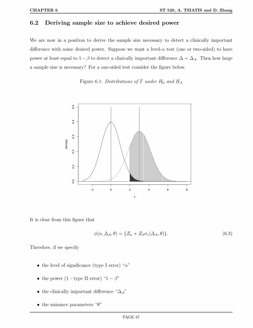
CHAPTER 6 ST 520, A. TSIATIS and D. Zhang
6.2 Deriving sample size to achieve desired power
We are now in a position to derive the sample size necessary to detect a clinically important
difference with some desired power. Suppose we want a level-α test (one or two-sided) to have
power at least equal to 1−β to detect a clinically important difference ∆ = ∆A. Then how large
a sample size is necessary? For a one-sided test consider the figure below.
Figure 6.1: Distributions of T under H0 and HA
−2 0 2 4 6 8
0.0
0.1
0.2
0.3
0.4
0.5
x
Den
sity
It is clear from this figure that
φ(n,∆A, θ) = Zα + Zβσ∗(∆A, θ). (6.3)
Therefore, if we specify
• the level of significance (type I error) “α”
• the power (1 - type II error) “1 − β”
• the clinically important difference “∆A”
• the nuisance parameters “θ”
PAGE 87

CHAPTER 6 ST 520, A. TSIATIS and D. Zhang
then we can find the value n which satisfies (6.3).
Consider the previous example of normally distributed response data where we use the t-test
to test for treatment differences in the mean response. If we randomize patients with equal
probability to the two treatments so that n1 = n2 ≈ n/2, then substituting (6.1) and (6.2) into
(6.3), we get∆A
σY
(4n
)1/2= (Zα + Zβ),
or
n1/2 =
(Zα + Zβ)σY × 2
∆A
n =
(Zα + Zβ)2σ2
Y × 4
∆2A
.
Note: For two-sided tests we use Zα/2 instead of Zα.
Example
Suppose we wanted to find the sample size necessary to detect a difference in mean response of
20 units between two treatments with 90% power using a t-test (two-sided) at the .05 level of
significance. We expect the population standard deviation of response σY to be about 60 units.
In this example α = .05, β = .10, ∆A = 20 and σY = 60. Also, Zα/2 = Z.025 = 1.96, and
Zβ = Z.10 = 1.28. Therefore,
n =(1.96 + 1.28)2(60)2 × 4
(20)2≈ 378 (rounding up),
or about 189 patients per treatment group.
6.3 Comparing two response rates
We will now consider the case where the primary outcome is a dichotomous response; i.e. each
patient either responds or doesn’t respond to treatment. Let π1 and π2 denote the population
response rates for treatments 1 and 2 respectively. Treatment difference is denoted by ∆ = π1−π2.
We wish to test the null hypothesis H0 : ∆ ≤ 0 (π1 ≤ π2) versus HA : ∆ > 0 (π1 > π2). In
some cases we may want to test the null hypothesis H0 : ∆ = 0 against the two-sided alternative
HA : ∆ 6= 0.
PAGE 88

CHAPTER 6 ST 520, A. TSIATIS and D. Zhang
A clinical trial is conducted where n1 patients are assigned treatment 1 and n2 patients are
assigned treatment 2 and the number of patients who respond to treatments 1 and 2 are denoted
by X1 and X2 respectively. As usual, we assume
X1 ∼ b(n1, π1)
and
X2 ∼ b(n2, π2),
and that X1 and X2 are statistically independent. If we let π1 = π2 +∆, then the distribution of
X1 and X2 is characterized by the test parameter ∆ and the nuisance parameter π2. If we denote
the sample proportions by p1 = X1/n1 and p2 = X2/n2, then we know from the properties of a
binomial distribution that
E(p1) = π1, var(p1) =π1(1 − π1)
n1,
E(p2) = π2, var(p2) =π2(1 − π2)
n2
.
This motivates the test statistic
Tn =p1 − p2
p(1 − p)
(1n1
+ 1n2
)1/2,
where p is the combined sample proportion for both treatments; i.e. p = (X1 +X2)/(n1 + n2).
Note: The statistic T 2n is the usual chi-square test used to test equality of proportions.
We can also write
p =p1n1 + p2n2
n1 + n2= p1
(n1
n1 + n2
)+ p2
(n2
n1 + n2
).
As such, p is an approximation (consistent estimator) for
π1
(n1
n1 + n2
)+ π2
(n2
n1 + n2
)= π,
where π is a weighted average of π1 and π2. Thus
Tn ≈ p1 − p2π(1 − π)
(1n1
+ 1n2
)1/2.
PAGE 89

CHAPTER 6 ST 520, A. TSIATIS and D. Zhang
The mean and variance of this test statistic under the null hypothesis ∆ = 0 (border of the null
and alternative hypotheses for a one-sided test) are
E∆=0(Tn) ≈ E∆=0
p1 − p2π(1 − π)
(1n1
+ 1n2
)1/2
=E∆=0(p1 − p2)
π(1 − π)
(1n1
+ 1n2
)1/2= 0,
var∆=0(Tn) ≈ var∆=0(p1) + var∆=0(p2)π(1 − π)
(1n1
+ 1n2
) =
π1(1−π1)
n1+ π2(1−π2)
n2
π(1 − π)
(1n1
+ 1n2
) .
But since π1 = π2 = π, we get var∆=0(Tn) = 1.
Because the distribution of sample proportions are approximately normally distributed, this
will imply that the distribution of the test statistic, which is roughly a linear combination of
independent sample proportions, will also be normally distributed. Since the normal distribution
is determined by its mean and variance, this implies that,
Tn(∆=0)∼ N(0, 1).
For the alternative hypothesis HA : ∆ = π1 − π2 = ∆A,
EHA(Tn) ≈ (π1 − π2)
π(1 − π)
(1n1
+ 1n2
)1/2=
∆Aπ(1 − π)
(1n1
+ 1n2
)1/2,
and using the same calculations for the variance as we did above for the null hypothesis we get
varHA(Tn) ≈
π1(1−π1)
n1+ π2(1−π2)
n2
π(1 − π)
(1n1
+ 1n2
) .
When n1 = n2 = n/2, we get some simplification; namely
π = (π1 + π2)/2 = (π2 + ∆A/2)
and
varHA(Tn) =
π1(1 − π1) + π2(1 − π2)
2π(1 − π).
Note: The variance under the alternative is not exactly equal to one, although, if π1 and π2 are
not very different, then it is close to one.
Consequently, with equal treatment allocation,
TnHA∼ N
∆Aπ(1 − π) 4
n
1/2,π1(1 − π1) + π2(1 − π2)
2π(1 − π)
.
PAGE 90

CHAPTER 6 ST 520, A. TSIATIS and D. Zhang
Therefore,
φ(n,∆A, θ) =∆A
π(1 − π) 4
n
1/2,
and
σ2∗ =
π1(1 − π1) + π2(1 − π2)
2π(1 − π),
where π1 = π2 + ∆A.
Using formula (6.3), the sample size necessary to have power at least (1−β) to detect an increase
of ∆A, or greater, in the population response rate of treatment 1 above the population response
rate for treatment 2, using a one-sided test at the α level of significance is
n1/2∆A
4π(1 − π)1/2= Zα + Zβ
π1(1 − π1) + π2(1 − π2)
2π(1 − π)
1/2
.
Hence
n =
Zα + Zβ
π1(1−π1)+π2(1−π2)
2π(1−π)
1/22
4π(1 − π)
∆2A
. (6.4)
Note: For two-sided tests we replace Zα by Zα/2.
Example: Suppose the standard treatment of care (treatment 2) has a response rate of about .35
(best guess). After collaborations with your clinical colleagues, it is determined that a clinically
important difference for a new treatment is an increase in .10 in the response rate. That is, a
response rate of .45 or larger. If we are to conduct a clinical trial where we will randomize patients
with equal allocation to either the new treatment (treatment 1) or the standard treatment, then
how large a sample size is necessary to detect a clinically important difference with 90% power
using a one-sided test at the .025 level of significance?
Note for this problem
• α = .025, Zα = 1.96
• β = .10 (power = .9), Zβ = 1.28
• ∆A = .10
• π2 = .35, π1 = .45, π = .40
PAGE 91

CHAPTER 6 ST 520, A. TSIATIS and D. Zhang
Substituting these values into (6.4) we get
n =
1.96 + 1.28
.45×.55+.35×.65
2×.40×.60
1/22
4 × .40 × .60
(.10)2≈ 1, 004,
or about 502 patients on each treatment arm.
6.3.1 Arcsin square root transformation
Since the binomial distribution may not be well approximated by a normal distribution, especially
when n is small (not a problem in most phase III clinical trials) or π is near zero or one,
other approximations have been suggested for deriving test statistics that are closer to a normal
distribution. We will consider the arcsin square root transformation which is a variance stabilizing
transformation. Before describing this transformation, I first will give a quick review of the
delta method for deriving distributions of transformations of estimators that are approximately
normally distributed.
Delta Method
Consider an estimator γn of a population parameter γ such that
γn ∼ N(γ,σ2
γ
n).
Roughly speaking, this means that
E(γn) ≈ γ
and
var(γn) ≈σ2
γ
n.
Consider the variable f(γn), where f(·) is a smooth monotonic function, as an estimator for f(γ).
Using a simple Taylor series expansion of f(γn) about f(γ), we get
f(γn) = f(γ) + f ′(γ)(γn − γ) + (small remainder term),
where f ′(γ) denotes the derivative df(γ)dγ
. Then
Ef(γn) ≈ Ef(γ) + f ′(γ)(γn − γ)
PAGE 92

CHAPTER 6 ST 520, A. TSIATIS and D. Zhang
= f(γ) + f ′(γ)E(γn − γ) = f(γ).
and
varf(γn) ≈ varf(γ) + f ′(γ)(γn − γ)
= f ′(γ)2var(γn) = f ′(γ)2
(σ2
γ
n
).
Thus
f(γn) ∼ N
(f(γ), f ′(γ)2
(σ2
γ
n
)).
Take the function f(·) to be the arcsin square root transformation; i.e
f(x) = sin−1(x)1/2.
If y = sin−1(x)1/2, then sin(y) = x1/2. The derivative dydx
is found using straightforward calculus.
That is,dsin(y)
dx=dx1/2
dx,
cos(y)dy
dx=
1
2x−1/2.
Since cos2(y) + sin2(y) = 1, this implies that cos(y) = 1 − sin2(y)1/2 = (1 − x)1/2. Therefore.
(1 − x)1/2 dy
dx=
1
2x−1/2,
ordy
dx=
1
2x(1 − x)−1/2 = f ′(x).
If p = X/n is the sample proportion, where X ∼ b(n, π), then var(p) = π(1−π)n
. Using the delta
method, we get that
varsin−1(p)1/2 ≈ f ′(π)2
π(1 − π)
n
,
=[1
2π(1 − π)−1/2
]2 π(1 − π)
n
,
=
1
4π(1 − π)
π(1 − π)
n
=
1
4n.
Consequently,
sin−1(p)1/2 ∼ N(sin−1(π)1/2,
1
4n
).
Note: The variance of sin−1(p)1/2 does not involve the parameter π, thus the term “variance
stabilizing”.
PAGE 93

CHAPTER 6 ST 520, A. TSIATIS and D. Zhang
The null hypothesis H0 : π1 = π2 is equivalent to H0 : sin−1(π1)1/2 = sin−1(π2)
1/2. This suggests
that another test statistic which could be used to test H0 is given by
Tn =sin−1(p1)
1/2 − sin−1(p2)1/2
(1
4n1+ 1
4n2
)1/2.
The expected value of Tn is
E(Tn) =Esin−1(p1)
1/2 −Esin−1(p2)1/2
(1
4n1+ 1
4n2
)1/2≈ sin−1(π1)
1/2 − sin−1(π2)1/2
(1
4n1+ 1
4n2
)1/2.
and the variance of Tn is
var(Tn) =varsin−1(p1)
1/2 − sin−1(p2)1/2(
14n1
+ 14n2
) =varsin−1(p1)
1/2 + varsin−1(p2)1/2(
14n1
+ 14n2
)
≈(
14n1
+ 14n2
)
(1
4n1+ 1
4n2
) = 1.
In addition to the variance stabilizing property of the arcsin square root transformation for the
sample proportion of a binomial distribution, this transformed sample proportion also has distri-
bution which is closer to a normal distribution. Since the test statistic Tn is a linear combination
of independent arcsin square root transformations of sample proportions, the distribution of Tn
will also be well approximated by a normal distribution. Specifically,
TnH0∼ N(0, 1)
TnHA∼ N
sin−1(π1)
1/2 − sin−1(π2)1/2
(1
4n1+ 1
4n2
)1/2, 1
.
If we take n1 = n2 = n/2, then the non-centrality parameter equals
φ(n,∆A, θ) = n1/2∆A,
where ∆A, the clinically important treatment difference, is parameterized as
∆A = sin−1(π1)1/2 − sin−1(π2)
1/2.
Consequently, if we parameterize the problem by considering the arcsin square root transfor-
mation, and use the test statistic above, then with equal treatment allocation, the sample size
necessary to detect a clinically important treatment difference of ∆A in the arcsin square root
PAGE 94

CHAPTER 6 ST 520, A. TSIATIS and D. Zhang
of the population proportions with power (1 − β) using a test (one-sided) at the α level of
significance, is derived by using (6.3); yielding
n1/2∆A = (Zα + Zβ),
n =(Zα + Zβ)2
∆2A
.
Remark: Remember to use radians rather than degrees in computing the arcsin or inverse of
the sine function. Some calculators give the result in degrees where π = 3.14159 radians is equal
to 180 degrees; i.e. radians=degrees
180× 3.14159.
If we return to the previous example where we computed sample size based on the proportions
test, but now instead use the formula for the arc sin square root transformation we would get
n =(1.96 + 1.28)2
sin−1(.45)1/2 − sin−1(.35)1/22=
(1.96 + 1.28)2
(.7353 − .6331)2= 1004,
or 502 patients per treatment arm. This answer is virtually identical to that obtained using
the proportions test. This is probably due to the relatively large sample sizes together with
probabilities being bounded away from zero or one where the normal approximation of either
the sample proportion of the arcsin square root of the sample proportion is good.
PAGE 95

CHAPTER 7 ST 520, A. TSIATIS and D. Zhang
7 Comparing More Than Two Treatments
Suppose we randomize patients to K > 2 treatments and are interested in testing whether there
are treatment differences in response. We proceed by positing the null hypothesis that there are
no treatment differences and then test this null hypothesis against the alternative hypothesis
that there exist some difference in response among the treatments.
Let us first consider the case where the response is dichotomous; i.e. the patient either responds
or doesn’t respond to treatment. Let π1, . . . , πK denote the population response rates for the K
treatments under study. The null hypothesis of no treatment differences is given by
H0 : π1 = π2 = . . . = πK .
The alternative hypothesis HA : states that the K population response rates “the π’s” are not
all equal.
To decide between H0 and HA, we conduct an experiment where we allocate n1, . . . , nK individ-
uals on each of the K treatments respectively and count the number that respond to each of the
treatments. Therefore, the data from such a clinical trial can be viewed as realizations of the
independent random variables X1, . . . , XK , where
Xi ∼ b(ni, πi), i = 1, . . . , K.
Each of the population response rates πi are estimated using the sample proportions pi =
Xi/ni, i = 1, . . . , K.
The strategy for decision making is to combine the data from such an experiment into a test
statistic for which larger values would provide increasing evidence against the null hypothesis.
In addition, the distribution of this test statistic, under the null hypothesis, is necessary in order
to gauge how extreme (evidence against H0) the observed data are compared to what may have
occurred by chance if the null hypothesis were true.
We begin by by first giving some general results regarding estimators that are normally dis-
tributed which will be used later for constructing test statistics.
PAGE 96

CHAPTER 7 ST 520, A. TSIATIS and D. Zhang
7.1 Testing equality using independent normally distributed estima-
tors
For i = 1, . . . , K, let the estimator θi be an unbiased estimator for the parameter θi which has a
normal distribution; i.e.
θi ∼ N(θi, σ2i ).
Assume σ2i is either known or can be estimated well (consistently) using the data.
Suppose we have K independent estimators θ1, . . . , θK of θ1, . . . , θK respectively such that
θi ∼ N(θi, σ2i ), i = 1, . . . , K.
If we assume that θ1 = . . . = θK (i.e. similar to a K-sample null hypothesis), then the weighted
estimator
ˆθ =
∑Ki=1wiθi∑Ki=1wi
, wi =1
σ2i
is the best unbiased estimator for the common value θ.
Remark: By best, we mean that among all functions of θ1, . . . , θK that are unbiased estimators
of θ, ˆθ (defined above) has the smallest variance.
In addition, when θ1 = . . . = θK ,, then the random variable
K∑
i=1
wi(θi − ˆθ)2 (7.1)
is distributed as a central chi-square distribution with K − 1 degrees of freedom. If the θi, i =
1, . . . , K are not all equal, thenK∑
i=1
wi(θi − ˆθ)2 (7.2)
is distributed as a non-central chi-square distribution with K − 1 degrees of freedom and non-
centrality parameter equal toK∑
i=1
wi(θi − θ)2, (7.3)
where
θ =
∑Ki=1wiθi∑Ki=1wi
.
Note: The non-centrality parameter is based on on the true population parameters.
PAGE 97

CHAPTER 7 ST 520, A. TSIATIS and D. Zhang
7.2 Testing equality of dichotomous response rates
How do the results above help us in formulating test statistics? Returning to the problem of
dichotomous response, the null hypothesis is
H0 : π1 = . . . = πK .
This is equivalent to
H0 : sin−1√π1 = . . . = sin−1√πK .
We showed in chapter 6 that if pi = Xi/ni is the sample proportion responding to treatment i,
then
sin−1√pi ∼ N(sin−1√πi,
1
4ni
).
Letting
• sin−1√pi take the role of θi
• sin−1√πi take the role of θi
• 14ni
be σ2i ; hence wi = 4ni
then by (7.1), the test statistic
Tn =K∑
i=1
4ni(sin−1√pi − Ap)
2, (7.4)
where
Ap =
∑Ki=1 nisin
−1√pi∑Ki=1 ni
,
is distributed as a central chi-square distribution with K − 1 degrees of freedom under the null
hypothesis H0.
This test statistic is a reasonable measure for assessing the strength of evidence of the alternative
hypothesis. If the population response rates πi, i = 1, . . . , K are all the same, then we would
expect the sample proportions pi to also be close to each other; in which case the test statistic
Tn would be near zero. The more different the pi’s are from each other the greater Tn would be.
Consequently, a reasonable strategy would be to reject the null hypothesis when the statistic Tn
PAGE 98

CHAPTER 7 ST 520, A. TSIATIS and D. Zhang
is sufficiently large. The degree of evidence is obtained by gauging the observed value of the test
statistic to the chi-square distribution with K − 1 degrees of freedom. If we denote by χ2α;K−1,
the (1−α)-th quantile of the central chi-square distribution with K−1 degrees of freedom, then
a test at the α-th level of significance can be obtained by rejecting H0 when
Tn ≥ χ2α;K−1.
Power and sample size calculations
In order to assess the power of the test, we need to know the distribution of the test statistic
under the alternative hypothesis. Suppose we entertain a specific alternative hypothesis that we
believe is clinically important to detect (more about this later). Say,
HA : π1 = π1A, . . . , πK = πKA,
where the πiA’s are not all equal. Using (7.2), the distribution of Tn is a non-central chi-square
with K − 1 degrees of freedom and non-centrality parameter given by (7.3), which in this case
equals
φ2 =K∑
i=1
4ni(sin−1√πiA − AπA)2, (7.5)
where
AπA =
∑Ki=1 nisin
−1√πiA∑Ki=1 ni
.
The level-α test rejects H0 when Tn ≥ χ2α;K−1. Therefore, the power of the test to detect HA
is the probability that a non-central chi-square distribution, with K − 1 degrees of freedom and
non-centrality parameter φ2, given by (7.5), exceed the value χ2α;K−1. See illustration below.
There are tables and/or computer packages available to carry out these probability calculations.
Sample size calculations
Suppose we allocate patients to each of the K treatments equally. Thus, on average, n1 = . . . =
nK = n/K, where n denotes the total sample size. In that case, the non-centrality parameter
(7.5) equals
φ2 =4n
K
K∑
i=1
(sin−1√πiA − AπA)2
, (7.6)
PAGE 99

CHAPTER 7 ST 520, A. TSIATIS and D. Zhang
Figure 7.1: Distributions of Tn under H0 and HA
0 5 10 15 20
0.00
0.05
0.10
0.15
0.20
0.25
x
Den
sity
nc=0nc=2
0 5 10 15 20
0.00
0.05
0.10
0.15
0.20
0.25
x
Den
sity
nc=0nc=5
where
AπA = K−1K∑
i=1
sin−1√πiA.
Note: AπA is just a simple averages of the sin−1√πiAs for the alternative of interest.
Let us define by
φ2(α, β,K − 1),
the value of the non-centrality parameter necessary so that a non-central chi-square distributed
random variable with K−1 degrees of freedom and non-centrality parameter φ2(α, β,K−1) will
exceed the value χ2α;K−1 with probability (1 − β). Values for φ2(α, β,K − 1) are given in tables
or derived from software packages for different values of α, β and degrees of freedom K − 1. For
illustration, we have copied a subset of such tables that we will use later in examples.
Thus, if we want a level-α test of the null hypothesis H0 : π1 = . . . = πK to have power (1 − β)
to detect the alternative hypothesis HA : π1 = π1A, . . . , πK = πKA (not all equal), then we need
the non-centrality parameter
4n
K
K∑
i=1
(sin−1√πiA − AπA)2
= φ2(α, β,K − 1),
PAGE 100
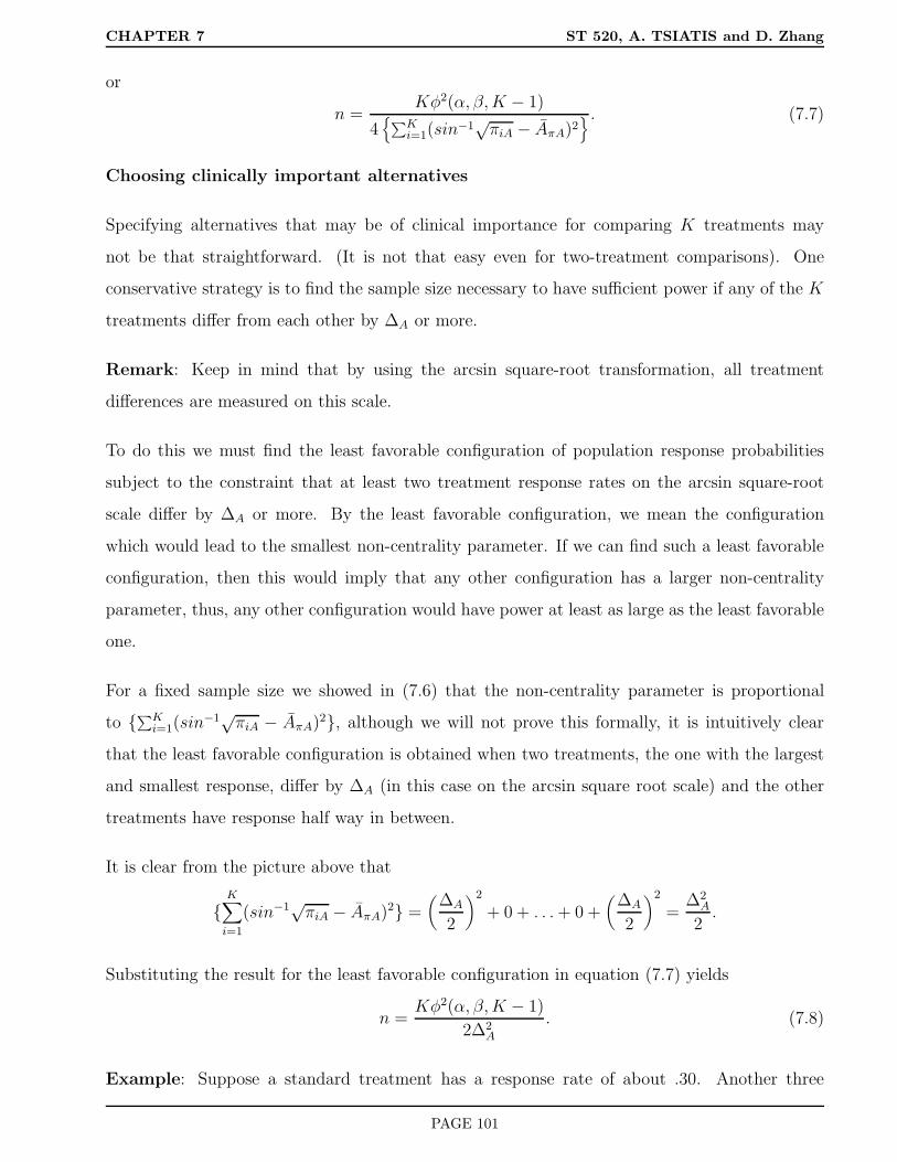
CHAPTER 7 ST 520, A. TSIATIS and D. Zhang
or
n =Kφ2(α, β,K − 1)
4∑K
i=1(sin−1√πiA − AπA)2
. (7.7)
Choosing clinically important alternatives
Specifying alternatives that may be of clinical importance for comparing K treatments may
not be that straightforward. (It is not that easy even for two-treatment comparisons). One
conservative strategy is to find the sample size necessary to have sufficient power if any of the K
treatments differ from each other by ∆A or more.
Remark: Keep in mind that by using the arcsin square-root transformation, all treatment
differences are measured on this scale.
To do this we must find the least favorable configuration of population response probabilities
subject to the constraint that at least two treatment response rates on the arcsin square-root
scale differ by ∆A or more. By the least favorable configuration, we mean the configuration
which would lead to the smallest non-centrality parameter. If we can find such a least favorable
configuration, then this would imply that any other configuration has a larger non-centrality
parameter, thus, any other configuration would have power at least as large as the least favorable
one.
For a fixed sample size we showed in (7.6) that the non-centrality parameter is proportional
to ∑Ki=1(sin
−1√πiA − AπA)2, although we will not prove this formally, it is intuitively clear
that the least favorable configuration is obtained when two treatments, the one with the largest
and smallest response, differ by ∆A (in this case on the arcsin square root scale) and the other
treatments have response half way in between.
It is clear from the picture above that
K∑
i=1
(sin−1√πiA − AπA)2 =(
∆A
2
)2
+ 0 + . . .+ 0 +(
∆A
2
)2
=∆2
A
2.
Substituting the result for the least favorable configuration in equation (7.7) yields
n =Kφ2(α, β,K − 1)
2∆2A
. (7.8)
Example: Suppose a standard treatment has a response rate of about .30. Another three
PAGE 101

CHAPTER 7 ST 520, A. TSIATIS and D. Zhang
treatments have been developed and it is decided to compare all of them in a head to head
randomized clinical trial. Equal allocation of patients to the four treatments is used so that
approximately n1 = n2 = n3 = n4 = n/4. We want the power of a test, at the .05 level of
significance, to be at least 90% if any of the other treatments has a response rate greater than
or equal to .40. What should we choose as the sample size?
For this example:
• α = .05
• 1 − β = .90, or β = .10
• K=4
• ∆A = sin−1√.40 − sin−1
√.30 = .1051
• φ2(.05, .10, 3) = 14.171 (derived from the tables provided)
Therefore by (7.8), we get
n =4 × 14.171
2(.1051)2= 2567,
or about 2567/4 = 642 patients per treatment arm.
7.3 Multiple comparisons
If we had done a two-treatment comparison for the previous example, and wanted 90% power
to detect a difference from .30 to .40 in response rate at the .05 (two-sided) level of significance,
then the sample size necessary is
n =2 × 10.507
2(.1051)2= 952,
or 476 patients per treatment arm.
For a four-treatment comparison, we needed 642 patients per treatment arm under similar pa-
rameter and sensitivity specifications. Why is there a difference and what are the implications
of this difference?
PAGE 102

CHAPTER 7 ST 520, A. TSIATIS and D. Zhang
We first note that when we test four treatments simultaneously, we can make six different pairwise
comparisons; i.e.
1 vs 2, 1 vs 3, 1 vs 4, 2 vs 3, 2 vs 4, 3 vs 4.
If each of these comparisons were made using separate studies, each at the same level and power
to detect the same alternative, then six studies would be conducted, each with 952 patients, or
952×6 = 5, 712 total patients. This is in contrast to the 2,567 patients used in the four-treatment
comparison.
This brings up the controversial issue regarding multiple comparisons. When conducting a clinical
trial with K treatments, K > 2, there are
K
2
possible pairwise comparisons that can be
made. If each comparison was made at the α level of significance, then even if the global null
hypothesis were true; (i.e. in truth, all treatments had exactly the same response rate), the
probability of finding at least one significant difference will be greater than α. That is, there is
an inflated study-wide type I error that is incurred due to the multiple comparisons.
Let’s be more specific. Denote by Tnij the test statistic used to compare treatment i to treatment
j, i < j, i, j = 1, . . . , K. There are
K
2
such pairwise treatment comparisons, each using the
test statistic
Tnij =2(sin−1√pi − sin−1√pj)
(1ni
+ 1nj
)1/2.
For a two-sample comparison, the level α test (two-sided) would reject the hypothesis H0ij : πi =
πj if
|Tnij| ≥ Zα/2,
That is,
PH0ij(|Tnij| ≥ Zα/2) = α.
However, if we made all possible pairwise treatment comparisons then the event of finding at
least one significant result is⋃
i<j, i,j=1,...,K
(|Tnij| ≥ Zα/2).
PAGE 103

CHAPTER 7 ST 520, A. TSIATIS and D. Zhang
It is clear that
PH0
⋃
i<j, i,j=1,...,K
(|Tnij| ≥ Zα/2) > PH0ij(|Tnij| ≥ Zα/2) = α.
If we are concerned about this issue and want to control the overall study-wide type I error
rate, then we would require greater evidence of treatment difference before declaring a pairwise-
treatment comparison to be significant. One simple, albeit conservative, strategy is to use Bon-
ferroni correction. This follows by noting that
PH0⋃
i<j
(|Tnij| ≥ c ≤∑
i<j
PH0ij(|Tnij | ≥ c).
There are
K
2
= K(K − 1)/2 elements in the sum on the right hand side of the formula
above. Therefore, if we choose the constant “c” so that each of the probabilities in the sum is
equal to
α/
K
2
,
then we are ensured that the probability on the left will be less than or equal to α. Since under
the null hypothesis Tnij follows a standard normal distribution, we choose
c = Zα/K(K−1).
Hence, with a Bonferroni correction, we would declare a pairwise treatment comparison (say
treatment i versus treatment j) significant if
|Tnij| ≥ Zα/K(K−1).
Using this as the convention, the probability of declaring any treatment pairwise comparison
significant under the null hypothesis is
PH0⋃
i<j
(|Tnij| ≥ Zα/K(K−1) ≤∑
i<j
PH0ij(|Tnij| ≥ Zα/K(K−1)) =
K
2
×2α/K(K−1) = α.
Example: If we were comparing four treatments, there would be six possible treatment compar-
isons. Using the Bonferroni method we would declare any such pairwise comparison significant
PAGE 104
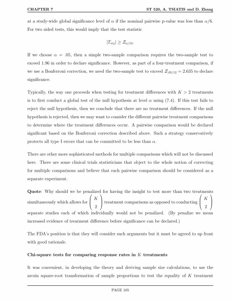
CHAPTER 7 ST 520, A. TSIATIS and D. Zhang
at a study-wide global significance level of α if the nominal pairwise p-value was less than α/6.
For two sided tests, this would imply that the test statistic
|Tnij | ≥ Zα/12.
If we choose α = .05, then a simple two-sample comparison requires the two-sample test to
exceed 1.96 in order to declare significance. However, as part of a four-treatment comparison, if
we use a Bonferroni correction, we need the two-sample test to exceed Z.05/12 = 2.635 to declare
significance.
Typically, the way one proceeds when testing for treatment differences with K > 2 treatments
is to first conduct a global test of the null hypothesis at level α using (7.4). If this test fails to
reject the null hypothesis, then we conclude that there are no treatment differences. If the null
hypothesis is rejected, then we may want to consider the different pairwise treatment comparisons
to determine where the treatment differences occur. A pairwise comparison would be declared
significant based on the Bonferroni correction described above. Such a strategy conservatively
protects all type I errors that can be committed to be less than α.
There are other more sophisticated methods for multiple comparisons which will not be discussed
here. There are some clinical trials statisticians that object to the whole notion of correcting
for multiple comparisons and believe that each pairwise comparison should be considered as a
separate experiment.
Quote: Why should we be penalized for having the insight to test more than two treatments
simultaneously which allows for
K
2
treatment comparisons as opposed to conducting
K
2
separate studies each of which individually would not be penalized. (By penalize we mean
increased evidence of treatment difference before significance can be declared.)
The FDA’s position is that they will consider such arguments but it must be agreed to up front
with good rationale.
Chi-square tests for comparing response rates in K treatments
It was convenient, in developing the theory and deriving sample size calculations, to use the
arcsin square-root transformation of sample proportions to test the equality of K treatment
PAGE 105
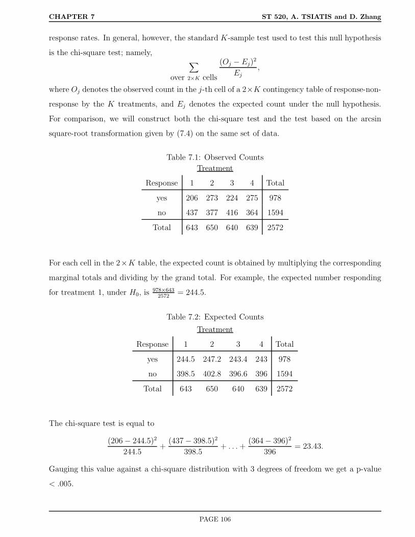
CHAPTER 7 ST 520, A. TSIATIS and D. Zhang
response rates. In general, however, the standard K-sample test used to test this null hypothesis
is the chi-square test; namely,∑
over 2×K cells
(Oj − Ej)2
Ej
,
where Oj denotes the observed count in the j-th cell of a 2×K contingency table of response-non-
response by the K treatments, and Ej denotes the expected count under the null hypothesis.
For comparison, we will construct both the chi-square test and the test based on the arcsin
square-root transformation given by (7.4) on the same set of data.
Table 7.1: Observed Counts
Treatment
Response 1 2 3 4 Total
yes 206 273 224 275 978
no 437 377 416 364 1594
Total 643 650 640 639 2572
For each cell in the 2×K table, the expected count is obtained by multiplying the corresponding
marginal totals and dividing by the grand total. For example, the expected number responding
for treatment 1, under H0, is 978×6432572
= 244.5.
Table 7.2: Expected Counts
Treatment
Response 1 2 3 4 Total
yes 244.5 247.2 243.4 243 978
no 398.5 402.8 396.6 396 1594
Total 643 650 640 639 2572
The chi-square test is equal to
(206 − 244.5)2
244.5+
(437 − 398.5)2
398.5+ . . .+
(364 − 396)2
396= 23.43.
Gauging this value against a chi-square distribution with 3 degrees of freedom we get a p-value
< .005.
PAGE 106

CHAPTER 7 ST 520, A. TSIATIS and D. Zhang
Using the same set of data we now construct the K-sample test (7.4) using the arcsin square-root
transformation.
Treatment i pi sin−1√pi
1 206/643=.32 .601
2 273/650=.42 .705
3 224/640=.35 .633
4 275/639=.43 .715
Ap =643 × .601 + 650 × .705 + 640 × .633 + 639 × .715
2572= .664,
and
Tn = 4643(.601− .664)2 + 650(.705 − .664)2 + 640(.633 − .664)2 + 639(.715 − .664)2 = 23.65.
Note: This is in good agreement with the chi-square test which, for the same set of data, gave
a value of 23.43. This agreement will occur when sample sizes are large as often is the case in
phase III clinical trials.
Example of pairwise comparisons
Suppose the data above were the results of a clinical trial. Now that we’ve established that it is
unlikely that the global null hypothesis H0 is true (p-value < .005), i.e. we reject H0, we may
want to look more carefully at the individual pairwise treatment differences.
Additionally, you are told that treatment 1 was the standard control and that treatments 2, 3
and 4 are new promising therapies. Say, that, up front in the protocol, it was stated that the
major objectives of this clinical trial were to compare each of the new treatments individually to
the standard control. That is, to compare treatments 1 vs 2, 1 vs 3, and 1 vs 4. If we want to
control the overall experimental-wide error rate to be .05 or less, then one strategy is to declare
any of the above three pairwise comparisons significant if the two-sided p-value were less than
.05/3=.0167. With a two-sided test, we would declare treatment j significantly different than
treatment 1, for j = 2, 3, 4 if the two-sample test
|Tn1j | ≥ Z.0167/2 = 2.385, j = 2, 3, 4.
PAGE 107

CHAPTER 7 ST 520, A. TSIATIS and D. Zhang
Remark: The exact same considerations would be made using a one-sided test at the .025 level
of significance. The only difference is that we would reject when Tnij ≥ 2.385. We must be
careful in defining Tn1j that the sign is such that large values are evidence against the one-sided
null hypothesis of interest.
With that in mind, we consider the test based on the arcsin square-root transformation
Tn1j = 2
(n1nj
n1 + nj
)1/2
(sin−1√pj − sin−1√p1).
Substituting the data above we get
Tn12 = 2(
643 × 650
643 + 650
)1/2
(.705 − .601) = 3.73∗
Tn13 = 2(
643 × 640
643 + 640
)1/2
(.633 − .601) = 1.14
Tn14 = 2(
643 × 639
643 + 639
)1/2
(.715 − .601) = 4.08∗
Thus we conclude that treatments 2 and 4 are significant better than treatment 1 (the standard
control).
Suppose all four treatments were experimental, in which case, all six pairwise comparisons are of
interest. To account for multiple comparisons, we would declare a pairwise comparison significant
if the two-sided p-value were less than .05/6=.0083. Thus we would reject the null hypothesis
H0ij : πi = πj when
|Tnij| ≥ Z.0083/2 = 2.635.
Note: the comparisons of treatments 1 vs 2 and 1 vs 4 would still be significant with this more
stringent criterion.
Rounding out the remaining pairwise comparisons we get
|Tn23| = |2(
650 × 640
650 + 640
)1/2
(.705 − .633)| = 2.59
|Tn24| = |2(
650 × 639
650 + 639
)1/2
(.705 − .715)| = 0.36
PAGE 108

CHAPTER 7 ST 520, A. TSIATIS and D. Zhang
|Tn34| = |2(
640 × 639
640 + 639
)1/2
(.633 − .715)| = 2.94 ∗ .
Clearly, treatments 2 and 4 are the better treatments, certainly better than control. The only
controversial comparison is treatment 2 versus treatment 3, where, we may not be able to conclude
that treatment 2 is significantly better than treatment 3 because of the conservativeness of the
Bonferroni correction
7.4 K-sample tests for continuous response
For a clinical trial where we randomize patients to one of K > 2 treatments and the primary
outcome is a continuous measurement, then our primary interest may be to test for differences in
the mean response among the K treatments. Data from such a clinical trial may be summarized
as realizations of the iid random vectors
(Yi, Ai), i = 1, . . . , n,
where Yi denotes the response (continuously distributed) for the i-th individual and Ai denotes
the treatment (1, 2, . . . , K) that the i-th individual was assigned. Let us denote the treatment-
specific mean and variance of response by
E(Yi|Ai = j) = µj, j = 1, . . . , K
and
var(Yi|Ai = j) = σ2Y j , j = 1, . . . , K.
Note:
1. Often, we make the assumption that the treatment-specific variances are equal; i.e. σ2Y 1 =
. . . = σ2Y K = σ2
Y , but this assumption is not necessary for the subsequent development.
2. Moreover, it is also often assumed that the treatment-specific distribution of response is
normally distributed with equal variances; i.e.
(Yi|Ai = j) ∼ N(µj , σ2Y ), j = 1, . . . , K
Again, this assumption is not necessary for the subsequent development.
PAGE 109

CHAPTER 7 ST 520, A. TSIATIS and D. Zhang
Our primary focus will be on testing the null hypothesis
H0 : µ1 = . . . = µK .
Let us redefine our data so that (Yij, i = 1, . . . , nj, j = 1, . . . , K) denotes the response for the i-th
individual within treatment j, and nj denotes the number of individuals in our sample assigned
to treatment j (n =∑K
j=1 nj). From standard theory we know that the treatment-specific sample
mean
Yj =nj∑
i=1
Yij/nj
is an unbiased estimator for µj and that asymptotically
Yj ∼ N(µj ,σ2
Y j
nj), j = 1, . . . , K.
Remark: If the Y ’s are normally distributed, then the above result is exact. However, with the
large sample sizes that are usually realized in phase III clinical trials, the asymptotic approxi-
mation is generally very good.
Also, we know that the treatment-specific sample variance
s2Y j =
∑nj
i=1(Yij − Yj)2
nj − 1
is an unbiased estimator for σ2Y j , and that asymptotically
Yj ∼ N(µj ,s2
Y j
nj), j = 1, . . . , K.
Remark: If the treatment specific variances are all equal, then the common variance is often
estimated using the pooled estimator
s2Y =
∑Kj=1
∑nj
i=1(Yij − Yj)2
n−K.
Returning to the general results of section 7.1 of the notes, we let
• Yj take the role of θj
• µj take the role of θj
PAGE 110

CHAPTER 7 ST 520, A. TSIATIS and D. Zhang
• s2
Y j
njtake the role of σ2
j ; hence wj =nj
s2
Y j
Using (7.1), we construct the test statistic
Tn =K∑
j=1
wj(Yj − ¯Y )2, (7.9)
where
¯Y =
∑Kj=1wjYj∑K
j=1wj
,
and wj =nj
s2
Y j.
For the case where we are willing to assume equal variances, we get that
Tn =
∑Kj=1 nj(Yj − ¯Y )2
s2Y
, (7.10)
where
¯Y =
∑Kj=1 njYj
n.
Under the null hypothesis H0, Tn is approximately distributed as a chi-square distribution with
K − 1 degrees of freedom. Under the alternative hypothesis
HA : µ1 = µ1A, . . . , µK = µKA
where the µjA’s are not all equal, Tn is approximately distributed as a non-central chi-square
distribution with K − 1 degrees of freedom and non-centrality parameter
φ2 =K∑
j=1
wj(µjA − µA)2, (7.11)
where
µA =
∑Kj=1wjµjA∑K
j=1wj
,
and wj =nj
σ2
Y j.
Assuming equal variances, we get the simplification
φ2 =
∑Kj=1 nj(µjA − µA)2
σ2Y
, (7.12)
where
µA =
∑Kj=1 njµjA
n.
PAGE 111

CHAPTER 7 ST 520, A. TSIATIS and D. Zhang
Remark: In the special case where the response data are exactly normally distributed with equal
treatment-specific variances, the test statistic Tn given by (7.10), under the null hypothesis, has a
distribution which is exactly equal to K−1 times a central F distribution with K−1 numerator
degrees of freedom and n−K denominator degrees of freedom. That is
Tn/(K − 1) =
∑Kj=1 nj(Yj − ¯Y )2/(K − 1)
s2Y
has an F distribution under the null hypothesis. This is exactly the test statistic that is used
for testing the equality of means in a one-way ANOVA model.
However, when the sample size n is large, we can use the test statistic given by (7.9), based on an
asymptotic chi-square distribution, to test H0 without making either the normality assumption
or the assumption of equal variances.
7.5 Sample size computations for continuous response
Let us consider the case where patients are allocated equally to the K treatments so that
n1 = . . . = nK = n/K,
and, for design purposes, we assume that the treatment specific variances are all equal which we
posit to be the value σ2Y . The question is how do we compute the sample size that is necessary to
have power (1−β) to detect an alternative where any two treatments population mean responses
may differ by ∆A or more? Using considerations almost identical to those used for testing equality
of response rates for dichotomous outcomes, we can find the least favorable configuration which
after substituting into (7.12), yields the non-centrality parameter
n∆2A
2Kσ2Y
. (7.13)
Hence, to obtain the desired power of (1 − β), we need
n∆2A
2Kσ2Y
= φ2(α, β,K − 1),
or
n =2Kσ2
Y φ2(α, β,K − 1)
∆2A
. (7.14)
Example:
PAGE 112

CHAPTER 7 ST 520, A. TSIATIS and D. Zhang
We expand on the example used for two-sample comparisons given on page 84 of the notes, but
now we consider K = 4 treatments. What is the sample size necessary to detect a significant
difference with 90% power or greater if any pairwise difference in mean treatment response is at
least 20 units using the K-sample test above at the .05 level of significance? We posit that the
standard deviation of response, assumed equal for all treatments, is σY = 60 units. Substituting
into formula (7.14), we get that
n =2 × 4 × (60)2 × 14.171
(20)2≈ 1020,
or about 1021/4=255 patients per treatment arm.
Remark: The 255 patients per arm represents an increase of 35% over the 189 patients per arm
necessary in a two-sample comparison (see page 84 of notes). This percentage increase is the
same as when we compare response rates for a dichotomous outcome with 4 treatments versus
2 treatments. This is not a coincidence, but rather, has to do with the relative ratio of the
non-centrality parameters for a test with 3 degrees of freedom versus a test with 1 degree of
freedom.
7.6 Equivalency Trials
The point of view we have taken thus far in the course is that of proving the superiority of one
treatment over another. It may also be the case that there already exists treatments that have
been shown to have benefit and work well. For example, a treatment may have been proven
to be significantly better than placebo in a clinical trial and has been approved by the FDA
and is currently on the market. However, there still may be room for other treatments to be
developed that may be equally effective. This may be the case because the current treatment or
treatments may have some undesirable side-effects, at least for some segment of the population,
who would like to have an alternative. Or perhaps, the cost of the current treatments are high
and some new treatments may be cheaper. In such cases, the company developing such a drug
would like to demonstrate that their new product is equally effective to those already on the
market or, at least, has beneficial effect compared to a placebo. The best way to prove that
the new product has biological effect is to conduct a placebo-controlled trial and demonstrate
superiority over the placebo using methods we have discussed. However, in the presence of
PAGE 113

CHAPTER 7 ST 520, A. TSIATIS and D. Zhang
established treatments that have already been proven effective, such a clinical trial would be
un-ethical. Consequently, the new treatment has to be compared to one that is already known
to be effective. The comparison treatment is referred to as an active or positive control.
The purpose of such a clinical trial would not necessarily be to prove that the new drug is better
than the positive control but, rather, that it is equivalent in some sense. Because treatment com-
parisons are based on estimates obtained from a sample of data and thus subject to variation, we
can never be certain that two products are identically equivalent in their efficacy. Consequently, a
new drug is deemed equivalent to a positive control if it can be proved with high probability that
it has response at least within some tolerable limit of the positive control. Of course the tricky
issue is to determine what might be considered a tolerable limit for purposes of equivalency. If
the positive control was shown to have some increase in mean response compared to placebo, say
∆∗, then one might declare a new drug equivalent to the positive control if it can be proved that
the mean response of the new drug is within ∆∗/2 of the mean response of the positive control
or better with high probability. Conservatively, ∆∗ may be chosen as the lower confidence limit
derived from the clinical trial data that compared the positive control to placebo. Let us assume
that the tolerable limit has been defined, usually, by some convention, or in negotiations of a
company with the regulatory agency. Let us denote the tolerable limit by ∆A.
Remark: In superiority trials we denoted by ∆A, the clinically important difference that we
wanted to detect with desired power. For equivalency trials, ∆A refers to the tolerable limit.
Let us consider the problem where the primary response is a dichotomous outcome. (Identical
arguments for continuous response outcomes can be derived analogously). Let π2 denote the
population response rate for the positive control, and π1 be the population response rate for the
new treatment.
Evaluating equivalency is generally stated as a one-sided hypothesis testing problem; namely,
H0 : π1 ≤ π2 − ∆A versus HA : π1 > π2 − ∆A.
If we denote by the parameter ∆ the treatment difference π1 − π2, then the null and alternative
hypotheses are
H0 : ∆ ≤ −∆A versus HA : ∆ > −∆A.
The null hypothesis corresponds to the new treatment being inferior to the positive control. This
PAGE 114

CHAPTER 7 ST 520, A. TSIATIS and D. Zhang
is tested against the alternative hypothesis that the new treatment is at least equivalent to the
positive control. As always, we need to construct a test statistic, Tn, which, when large, would
provide evidence against the null hypothesis and whose distribution at the border between the
null and alternative hypotheses (i.e. when π1 = π2 − ∆A) is known. Letting p1 and p2 denote
the sample proportion that respond on treatments 1 and 2 respectively, an obvious test statistic
to test H0 versus HA is
Tn =p1 − p2 + ∆A√
p1(1−p1)n1
+ p2(1−p2)n2
,
where n1 and n2 denote the number of patients allocated to treatments 1 and 2 respectively.
This test statistic was constructed so that at the border of the null and alternative hypotheses;
i.e. when π1 = π2 −∆A, the distribution of Tn will be approximately a standard normal; that is
Tn(π1=π2−∆A)∼ N(0, 1).
Clearly, larger values of Tn give increasing evidence that the null hypothesis is not true in favor
of the alternative hypothesis. Thus, for a level α test, we reject when
Tn ≥ Zα.
With this strategy, one is guaranteed with high probability (≥ 1 − α) that the drug will not be
approved if, in truth, it is not at least equivalent to the positive control.
Remark: Notice that we didn’t use the arcsin square-root transformation for this problem. This
is because the arcsin square-root is a non-linear transformation; thus, a fixed difference of ∆A in
response probabilities between two treatments (hypothesis of interest) does not correspond to a
fixed difference on the arcsin square-root scale.
Sample size calculations for equivalency trials
In computing sample sizes for equivalency trials, one usually considers the power, i.e the prob-
ability of declaring equivalency, if, in truth, π1 = π2. That is, if, in truth, the new treatment
has a response rate that is as good or better than the positive control, then we want to declare
equivalency with high probability, say (1 − β). To evaluate the power of this test to detect the
alternative (π1 = π2), we need to know the distribution of Tn when π1 = π2.
PAGE 115

CHAPTER 7 ST 520, A. TSIATIS and D. Zhang
Because
Tn =(p1 − p2 + ∆A)√p1(1−p1)
n1+ p2(1−p2)
n2
≈ p1 − p2 + ∆A√π1(1−π1)
n1+ π2(1−π2)
n2
,
straightforward calculations can be used to show that
E(Tn)(π1=π2=π)≈ ∆A√
π(1 − π)(
1n1
+ 1n2
) ,
and
var(Tn)(π1=π2=π)≈ 1.
Hence
Tn(π1=π2=π)∼ N
∆A√π(1 − π)
(1n1
+ 1n2
) , 1
,
and the non-centrality parameter equals
φ(·) =∆A√
π(1 − π)(
1n1
+ 1n2
) .
If n1 = n2 = n/2, then
φ(·) =∆A√
π(1 − π)(
4n
) .
To get the desired power, we solve
∆A√π(1 − π)
(4n
) = Zα + Zβ
or
n =(Zα + Zβ)2 × 4π(1 − π)
∆2A
. (7.15)
Generally, it requires larger sample sizes to establish equivalency because the tolerable limit ∆A
that the regulatory agency will agree to is small. For example, a pharmaceutical company has
developed a new drug that they believe has similar effects to drugs already approved and decides
to conduct an equivalency trial to get approval from the FDA to market the new drug. Suppose
the clinical trial that was used to demonstrate that the positive control was significantly better
than placebo had a 95% confidence interval for ∆ (treatment difference) that ranged from .10-
.25. Conservatively, one can only be relatively confident that this new treatment has a response
rate that exceeds the response rate of placebo by .10. Therefore the FDA will only allow a new
PAGE 116

CHAPTER 7 ST 520, A. TSIATIS and D. Zhang
treatment to be declared equivalent to the positive control if the company can show that their
new drug has a response rate that is no worse than the response rate of the positive control
minus .05. Thus they require a randomized two arm equivalency trial to compare the new drug
to the positive control with a type I error of α = .05. The response rate of the positive control is
about .30. (This estimate will be used for planning purposes). The company believes their drug
is similar but probably not much better than the positive control. Thus, they want to have good
power, say 90%, that they will be successful (i.e. be able to declare equivalency by rejecting H0)
if, indeed, their drug was equally efficacious. Thus they use formula (7.15) to derive the sample
size
n =(1.64 + 1.28)2 × 4 × .3 × .7
(.05)2= 2864,
or 1432 patients per treatment arm.
PAGE 117

CHAPTER 8 ST 520, A. TSIATIS and D. Zhang
8 Causality, Non-compliance and Intent-to-treat
8.1 Causality and Counterfactual Random Variables
Throughout the course, we’ve repeatedly said that randomization allows us to make causal
statements regarding the effect of treatment on the primary response of interest. In this section,
we will be more formal. The actual definition of cause and effect has been hotly debated over
the years especially by philosophers. We will take a particular point of view using what are
called counterfactual random variables. As usual, we consider a super-population of individuals
that we are interested in and assume that the participants in a clinical trial represent a random
sample from this population. For concreteness, let us consider a clinical trial which will compare
a new treatment (treatment 1) to no treatment or placebo (treatment 0).
We define the counterfactual random variable Y ∗1 to denote the response (may be a binary
or continuous outcome) that a randomly selected individual from our population if, possibly
contrary to fact, that individual received treatment 1 (new treatment). Similarly, we define the
counterfactual random variable Y ∗0 to denote the response that a randomly selected individual
from our population if, possibly contrary to fact, that individual received treatment 0 (placebo).
We imagine the existence of both random variables (Y ∗0 , Y
∗1 ) even though in actuality it would
be impossible to observe both responses on any given individual. Thus the term counterfactual
or “contrary to fact”. At the individual level, we say that treatment causes the effect Y ∗1 − Y ∗
0 .
Clearly, if an individual knew their response to both treatment and placebo, then he/she would
choose whichever gave the better response. Of course, this is not possible at the individual level
but perhaps we can look at this question at the population level. That is, we will consider the
population mean causal effect; namely ∆ = E(Y ∗1 −Y ∗
0 ) = E(Y ∗1 )−E(Y ∗
0 ). If ∆ is positive, then
on average the response on treatment 1 will be better than on treatment 0. At the individual
level this will not necessarily imply that any specific individual will be guaranteed to benefit,
but on average, the population as a whole will benefit.
Knowledge of the average causal effect at the population level, if it can be obtained or estimated, is
still useful at the individual level. Say, for example, it has been proved that ∆ is positive; i.e. that
on average treatment 1 is better than treatment 0, then in the absence of any additional a-priori
knowledge that would distinguish one individual from the other, the best treatment choice for any
PAGE 118

CHAPTER 8 ST 520, A. TSIATIS and D. Zhang
individual in the population is treatment 1. If there are additional pre-treatment characteristics
that can distinguish individuals from each other; say, covariates X (e.g. age, gender, race,
etc.), then we would be interested in knowing or estimating the conditional expectation ∆(x) =
E(Y ∗1 − Y ∗
0 |X = x). If such a relationship were known, then the best choice for an individual
whoseX characteristics were equal to x, without any other additional knowledge of the individual,
would be to choose treatment 1 if ∆(x) > 0 and to choose treatment 0 if ∆(x) < 0. The question
then becomes whether we can estimate the average causal treatment effect ∆ or the average
causal treatment effect conditional on X = x, ∆(x), from a sample of individuals in a clinical
trial.
The data that we actually get to observe from a clinical trial can be summarized by (Yi, Ai, Xi), i =
1, . . . , n, where, for a randomly selected individual i from our population, Ai = (0, 1) denotes
the treatment assignment, Yi denotes the response and Xi denotes any additional characteristics,
(prognostic factors) that are collected on the individual prior to treatment assignment (baseline
characteristics). We will refer to these as the observable random variables. We distinguish here
between the observed response Yi for the i-th individual and the counterfactual responses Y ∗1i, Y
∗0i.
We will, however, make the reasonable assumption that
Yi = Y ∗1iI(Ai = 1) + Y ∗
0iI(Ai = 0), (8.1)
where I(·) denotes the indicator function of an event; that is, if the event is true this function
equals 1, otherwise, it equals 0. In words, assumption (8.1) means that the observed response Yi
equals the counterfactual response Y ∗1i if the i-th individual were assigned treatment 1; whereas,
the observed response would equal the counterfactual response Y ∗0i if the i-th individual were
assigned treatment 0.
Traditional statistical methods and models allow us to make associational relationships regarding
the probability distribution of the observable random variables. For example, we can posit
regression models that allow us to estimate relationships such as E(Yi|Ai, Xi). However, these
associational relationships are not the causal relationships that we argue are the important
parameters of interest. Thus, the question is under what conditions or assumptions can we
estimate causal parameters such as ∆ or ∆(x), from the sample of observable data. This is
where randomization plays a key role. Since the assignment of treatment to the patient in a
randomized study is made using a random number generator, it is completely independent of
PAGE 119
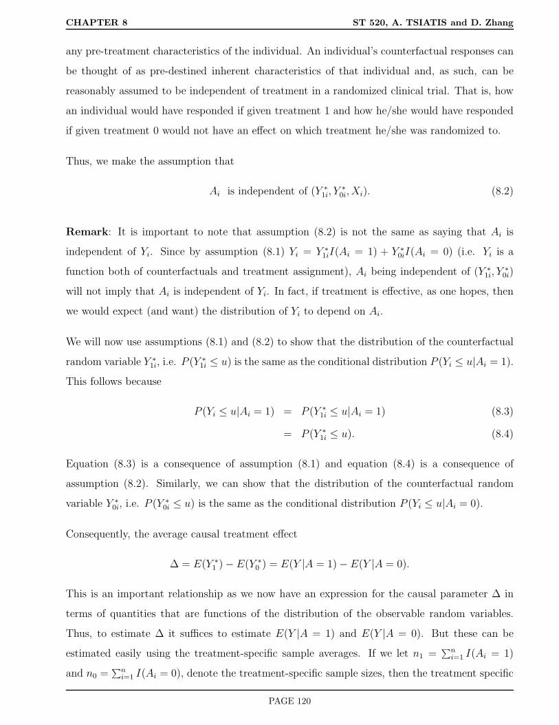
CHAPTER 8 ST 520, A. TSIATIS and D. Zhang
any pre-treatment characteristics of the individual. An individual’s counterfactual responses can
be thought of as pre-destined inherent characteristics of that individual and, as such, can be
reasonably assumed to be independent of treatment in a randomized clinical trial. That is, how
an individual would have responded if given treatment 1 and how he/she would have responded
if given treatment 0 would not have an effect on which treatment he/she was randomized to.
Thus, we make the assumption that
Ai is independent of (Y ∗1i, Y
∗0i, Xi). (8.2)
Remark: It is important to note that assumption (8.2) is not the same as saying that Ai is
independent of Yi. Since by assumption (8.1) Yi = Y ∗1iI(Ai = 1) + Y ∗
0iI(Ai = 0) (i.e. Yi is a
function both of counterfactuals and treatment assignment), Ai being independent of (Y ∗1i, Y
∗0i)
will not imply that Ai is independent of Yi. In fact, if treatment is effective, as one hopes, then
we would expect (and want) the distribution of Yi to depend on Ai.
We will now use assumptions (8.1) and (8.2) to show that the distribution of the counterfactual
random variable Y ∗1i, i.e. P (Y ∗
1i ≤ u) is the same as the conditional distribution P (Yi ≤ u|Ai = 1).
This follows because
P (Yi ≤ u|Ai = 1) = P (Y ∗1i ≤ u|Ai = 1) (8.3)
= P (Y ∗1i ≤ u). (8.4)
Equation (8.3) is a consequence of assumption (8.1) and equation (8.4) is a consequence of
assumption (8.2). Similarly, we can show that the distribution of the counterfactual random
variable Y ∗0i, i.e. P (Y ∗
0i ≤ u) is the same as the conditional distribution P (Yi ≤ u|Ai = 0).
Consequently, the average causal treatment effect
∆ = E(Y ∗1 ) − E(Y ∗
0 ) = E(Y |A = 1) − E(Y |A = 0).
This is an important relationship as we now have an expression for the causal parameter ∆ in
terms of quantities that are functions of the distribution of the observable random variables.
Thus, to estimate ∆ it suffices to estimate E(Y |A = 1) and E(Y |A = 0). But these can be
estimated easily using the treatment-specific sample averages. If we let n1 =∑n
i=1 I(Ai = 1)
and n0 =∑n
i=1 I(Ai = 0), denote the treatment-specific sample sizes, then the treatment specific
PAGE 120
CHAPTER 8 ST 520, A. TSIATIS and D. Zhang
sample averages
Y1 =n∑
i=1
YiI(Ai = 1)/n1; Y0 =n∑
i=1
YiI(Ai = 0)/n0,
are unbiased estimators for E(Y |A = 1) and E(Y |A = 0) respectively. Thus, an unbiased
estimator for the causal treatment effect ∆ can be derived from a randomized study using
∆ = Y1 − Y0.
Remark: The above arguments make formal what is intuitively obvious; that is, we can use the
difference in the treatment-specific sample averages in a randomized clinical trial to estimate the
true population treatment effect.
Similar arguments can also be used to show that in a randomized trial
∆(x) = E(Y ∗1 − Y ∗
0 |X = x) = E(Y |A = 1, X = x) − E(Y |A = 0, X = x).
Thus, to estimate ∆(x), it suffices to estimate the conditional mean of the observable random
variables E(Y |A,X). This can be accomplished, say, by positing a model (either linear or
nonlinear with or without interaction terms)
E(Y |A,X) = µ(A,X, β),
in terms of unknown parameters β. For example, if X is a single covariate, we might consider a
linear model with treatment-covariate interactions such as
µ(A,X, β) = β0 + β1A + β2X + β3AX. (8.5)
From a sample of data (Yi, Ai, Xi), i = 1, . . . , n we can estimate the parameters β in our model
using standard statistical techniques such as least squares or weighted least squares. If we denote
the estimator by β, then the estimate for ∆(x) is given by
∆(x) = µ(1, x, β) − µ(0, x, β).
For example, if we used model (8.5), then
∆(x) = (β0 + β1 + β2x+ β3x) − (β0 + β2x) = β1 + β3x.
PAGE 121
CHAPTER 8 ST 520, A. TSIATIS and D. Zhang
8.2 Noncompliance and Intent-to-treat analysis
The arguments outlined above assume that patients receive and take the treatment (or control)
to which they are randomized. In many clinical trials, if not most, this is rarely the case. There
is almost always some form of noncompliance from the intended treatment regimen.
Some reasons for a departure from the ideal treatment schedule are:
• A refusal by the patient to start or continue the assigned treatment, perhaps because of
side effects or a belief that the treatment is ineffective
• A failure to comply with detailed instructions, for example, drug dosage, or to attend
examinations when requested to do do
• A change of treatment imposed by the physician for clinical reasons, usually occurrence of
adverse effects or deterioration of patient’s health
• An administrative error. In its most extreme form this may be the implementation of the
wrong treatment.
How should we analyze the data when there is noncompliance? Some strategies that have been
proposed and is a source of much debate between clinicians and statisticians include
• Intent-to-Treat Analysis (As randomized)
Everyone is included in the analysis and the comparison of treatments is based on the
difference of the average response between the randomized groups ignoring the fact that
some patients were non-compliant.
• As-treated analysis
This type of analysis takes on various forms, but the general idea is to compare only
those patients who fully complied with their assigned treatment regimen and exclude non
compliers from the analysis.
PAGE 122

CHAPTER 8 ST 520, A. TSIATIS and D. Zhang
General Dogma of Clinical Trials
The exclusion of patients from the analysis should not allow the potential of bias in the treatment
comparisons. Thus, exclusions based on post-randomization considerations, such as noncompli-
ance, are not allowed for the primary analysis.
To illustrate some of the difficulties that can result from noncompliance, we consider some results
from a study conducted by the Coronary Drug Project which was published in the New England
Journal of Medicine, October, 1980, 303: 1038-1041. This study was a double-blind placebo-
controlled clinical trial comparing Clofibrate to Placebo.
Table 8.1: Intent-to-Treat Analysis
Clofibrate Placebo
5 year mortality .18 .19
rate
number of patients 1065 2695
Table 8.2: Clofibrate Patients Only
Adherence 5 year Number
(% of capsules taken) mortality rate patients
Poor (< 80%) .25 357
Good (> 80%) .15 708
p-value=.001
Table 8.3: Clofibrate and Placebo Patients
Clofibrate Placebo
5 year number 5 year number
Adherence mortality patients mortality patients
Poor (< 80%) .25 357 .28 882
Good (> 80%) .15 708 .15 1813
PAGE 123
CHAPTER 8 ST 520, A. TSIATIS and D. Zhang
It is clear from this data that patients who comply are prognostically different from those who
do not comply. Therefore, analyzing the data according to as-treated may lead to severe biases
because we cannot separate out the prognostic effect of noncompliance from the prognostic effect
of treatment. An intent-to-treat analysis does not suffer from this type of potentially biased
exclusions; nonetheless, we intuitively realize that when some patients do not comply with the
intended treatment then an intent-to-treat analysis would diminish the effect of a treatment. Let
us look at this issue a bit more carefully with the use of counterfactual modeling.
8.3 A Causal Model with Noncompliance
We consider the following simple example for illustrative purposes.
• A randomized study is conducted where patients are randomized with equal probability to
active drug (treatment 1) or placebo (control) (treatment 0)
• Response is dichotomous; i.e. a patient either responds or not
• The main goal of the clinical trial is to estimate the difference in the probability of response
between active drug and placebo
• Patients may not comply with their assigned treatment
• For simplicity, we assume that everyone either takes their assigned treatment or not (partial
compliance is not considered)
• A simple assay can be conducted on patients that were randomized to receive active drug
to see if they complied or not
• Patients assigned to placebo do not have access to the study drug
• Compliance cannot be determined for patients randomized to placebo
Counterfactual and observable random variables
The problem above can be conceptualized as follows:
PAGE 124

CHAPTER 8 ST 520, A. TSIATIS and D. Zhang
Let the counterfactual random variables (Y ∗1 , Y
∗0 ) denote the response (1 if they respond, 0 if they
don’t respond) of a randomly selected individual in our population if they received treatment 1 or
treatment 0 respectively. Also let C denote the counterfactual random variable corresponding to
whether or not a randomly selected individual in our population would comply or not C = (1, 0)
if offered the new treatment. We refer to this as a counterfactual random variable because we
will not know the compliance status if offered new treatment for patients randomized to placebo.
Some of the population parameters associated with these counterfactuals are
• A complier (COM) and a noncomplier (NC) refer only to patients complying or not if
offered active drug
• θ = P (C = 1) denotes the population probability of complying
• πCOM1 = P (Y ∗
1 = 1|C = 1) denotes the population probability of response among compliers
if given active drug,
• πNC1 = P (Y ∗
1 = 1|C = 0) denotes the population probability of response among noncom-
pliers if given active drug
• πCOM0 = P (Y ∗
0 = 1|C = 1) denotes the population probability of response among compliers
if given placebo
• πNC0 = P (Y ∗
0 = 1|C = 0) denotes the population probability of response among noncom-
pliers if given placebo
Table 8.4: Hypothetical Population
COMPLIERS NONCOMPLIERS
θ (1 − θ)
Treatment πCOM1 πNC
1
Placebo πCOM0 πNC
0
Difference ∆COM ∆NC
As we argued previously, it is not reasonable to assume that (Y ∗1 , Y
∗0 ) are independent of C.
Thus, we would not expect πCOM1 = πNC
1 or πCOM0 = πNC
0 .
PAGE 125

CHAPTER 8 ST 520, A. TSIATIS and D. Zhang
Using this notation and some simple probability calculations we get that
E(Y ∗1 ) = P (Y ∗
1 = 1) = πCOM1 θ + πNC
1 (1 − θ) = π1
and
E(Y ∗0 ) = P (Y ∗
0 = 1) = πCOM0 θ + πNC
0 (1 − θ) = π0.
Therefore, the average causal treatment effect equals
∆ = E(Y ∗1 ) − E(Y ∗
0 ) = π1 − π0 = ∆COMθ + ∆NC(1 − θ).
The question is whether we can estimate these counterfactual parameters using the data we get to
observe from a randomized clinical trial when there is noncompliance. We denote the observable
data as (Y,A,AC), where A = (1, 0) denotes the treatment that a patient is randomized to. C
will denote the indicator of compliance which is only observed for patients randomized to active
treatment. Thus the possible values that (A,AC) can take are
• (0, 0) corresponding to a patient randomized to placebo
• (1, 1) corresponding to a patient randomized to active treatment who complies
• (1, 0) corresponding to a patient randomized to active treatment who does not comply
Finally, the observable random variable Y = (0, 1) denotes the observed response.
Remark: In our scenario, if a patient is randomized to placebo, then that patient will not
receive active treatment; whereas, if a patient is randomized to active treatment, then he/she
will receive active treatment only if he/she complies; otherwise if the patient doesn’t comply,
then he/she will not receive active treatment.
The above considerations lead to the following reasonable assumptions:
Y = Y ∗0 I(A = 0) + Y ∗
1 I(A = 1, C = 1) + Y ∗0 I(A = 1, C = 0)
and because of randomization
A is independent of (Y ∗1 , Y
∗0 , C).
PAGE 126

CHAPTER 8 ST 520, A. TSIATIS and D. Zhang
Because of these assumptions, we can equate some of the parameters regarding the distribution
of the observable random variables to the parameters of the distribution of the counterfactual
random variables.
Namely,
P (C = 1|A = 1) = P (C = 1) = θ
P (Y = 1|A = 0) = P (Y ∗0 = 1|A = 0) = P (Y ∗
0 = 1) = π0
P (Y = 1|A = 1, C = 1) = P (Y ∗1 = 1|A = 1, C = 1) = P (Y ∗
1 = 1|C = 1) = πCOM1
P (Y = 1|A = 1, C = 0) = P (Y ∗0 = 1|A = 1, C = 0) = P (Y ∗
0 = 1|C = 0) = πNC0
Note: All the probabilities above can be estimated using the corresponding sample proportions
in a clinical trial.
Interestingly, since we can get estimates of π0, πNC0 and θ, then we can use the relationship that
π0 = πCOM0 θ + πNC
0 (1 − θ)
to get that
πCOM0 =
π0 − πNC0 (1 − θ)
θ.
In fact, the only counterfactual probability that cannot be estimated is πNC1 as it is impossible
to deduce the proportion of noncompliers who would have responded if forced to take treatment.
Intent-to-treat analysis
In an intent-to-treat analysis, where we compare the response rate among patients randomized
to active drug to the response rate among patients randomized to placebo, we are estimating
∆ITT = P (Y = 1|A = 1) − p(Y = 1|A = 0).
Again, by the assumptions made and some probability calculations we get
PAGE 127
CHAPTER 8 ST 520, A. TSIATIS and D. Zhang
P (Y = 1|A = 1) = P (Y = 1|A = 1, C = 1)P (C = 1|A = 1)
+ P (Y = 1|A = 1, C = 0)P (C = 0|A = 1)
= P (Y ∗1 = 1|A = 1, C = 1)P (C = 1|A = 1) + P (Y ∗
0 = 1|A = 1, C = 0)P (C = 0|A = 1)
= P (Y ∗1 = 1|C = 1)P (C = 1) + P (Y ∗
0 = 1|C = 0)P (C = 0)
= πCOM1 θ + πNC
0 (1 − θ) (8.6)
Also
P (Y = 1|A = 0) = P (Y ∗0 = 1|A = 0) = P (Y ∗
0 = 1) = π0 = πCOM0 θ + πNC
0 (1 − θ). (8.7)
Subtracting (8.7) from (8.6) we get that
∆ITT = P (Y = 1|A = 1) − P (Y = 1|A = 0) = (πCOM1 − πCOM
0 )θ,
or
∆ITT = ∆COMθ. (8.8)
Recall that
∆COM = P (Y ∗1 = 1|C = 1) − P (Y ∗
0 = 1|C = 1) = E(Y ∗1 − Y ∗
0 |C = 1)
is the difference in the mean counterfactual responses between treatment and placebo among
patients that would comply with treatment. As such, ∆COM is a causal parameter and some
argue that it is the causal parameter of most interest since the patients that will benefit from a
new treatment are those who will comply with the new treatment. Equation (8.8) makes it clear
that the intention-to-treat analysis will yield an estimator which diminishes a causal treatment
effect. In fact, since we are able to estimate the parameter θ, the probability of complying if
offered the new treatment, then the causal parameter ∆COM can be identified using parameters
from the observable random variables; namely
∆COM =P (Y = 1|A = 1) − P (Y = 1|A = 0)
P (C = 1|A = 1). (8.9)
Since all the quantities on the right hand side of (8.9) are easily estimated from the data of a
clinical trial, this means we can estimate the causal parameter ∆COM .
PAGE 128
CHAPTER 8 ST 520, A. TSIATIS and D. Zhang
Remarks
• If the null hypothesis of no treatment effect is true; namely
H0 : ∆COM = ∆NC = ∆ = 0
– The intent to treat analysis, which estimates (∆COMθ), gives an unbiased estimator
of treatment difference (under H0) and can be used to compute a valid test of the null
hypothesis
• If we were interested in estimating the causal parameter ∆COM , the difference in response
rate between treatment and placebo among compliers only, then
– the intent to treat analysis gives an underestimate of this population causal effect
• Since there are no data available to estimate πNC1 , we are not able to estimate ∆NC or ∆
As-treated analysis
In one version of an as treated analysis we compare the response rate of patients randomized to
receive active drug who comply to all patients randomized to receive placebo. That is, we
compute
∆AT = πCOM1 − π0.
Since π0 = πCOM0 θ + πNC
0 (1 − θ), after some algebra we get that
∆AT = ∆ + (πCOM1 − πNC
1 )(1 − θ),
where ∆ denotes the average causal treatment effect. This makes clear that when there is
noncompliance, (θ < 1), the as-treated analysis will yield an unbiased estimate of the average
causal treatment effect only if πCOM1 = πNC
1 . As we’ve argued previously, this assumption is not
generally true and hence the as-treated analysis can result in biased estimation even under the
null hypothesis.
Some Additional Remarks about Intention-to-Treat (ITT) Analyses
• By not allowing any exclusions, we are preserving the integrity of randomization
PAGE 129

CHAPTER 8 ST 520, A. TSIATIS and D. Zhang
• With the use of ITT, we are comparing the policy of using treatment A where possible to
the policy of using treatment B (control) where possible
• If the intended treatments are alway used, there is of course no problem
• If the treatments are rarely used, then the clinical trial will carry little information about
the true effect of A versus B, but a great deal of information about the difficulties to use
them
• The approach of comparing policies of intentions rather than rigorously standardized regi-
mens may be a more realistic statement of the purpose of the investigation
– This is the pragmatic approach to a clinical trial
– As compared to the explanatory approach which looks for a measure of effectiveness
rather than efficacy.
• The estimate of the causal effect ∆COM is larger than the intent-to-treat estimator ∆ITT ,
but it also has proportionately larger standard deviation. Thus use of this estimator as
a basis for a test of the null hypothesis yields the same significance level as a standard
intent-to-treat analysis
PAGE 130

CHAPTER 9 ST 520, A. TSIATIS and D. Zhang
9 Survival Analysis in Phase III Clinical Trials
In chronic disease clinical trials; e.g. Cancer, AIDS, Cardiovascular disease, Diabetes, etc., the
primary endpoint is often time to an event, such as time to death, time to relapse of disease, etc.
For such clinical trials the major focus is to compare the distribution of time to event among
competing treatments.
Typically, the clinical trials occur over a finite period of time and consequently the time to event
is not ascertained on all the patients in the study. This results in censored data. In addition,
since patients enter the clinical trial at different calendar times (staggered entry), the length
of follow-up varies by the individual. The combination of censoring and differential follow-up
creates some unusual difficulties in the analysis of such data that do not allow standard statistical
techniques to be used. Because of this, a whole new research area in Statistics has emerged to
study such problems. This is called Survival Analysis or Censored Survival Analysis. A
brief introduction of Survival Analysis will be given in this chapter, but for a more thorough
study of this area I recommend the course in Applied Survival Analysis offered every Spring
semester and for individuals interested in a more rigorous treatment of the subject there is a
course on Advanced Survival Analysis offered every other year.
In survival analysis, the endpoint of interest is time to an event which we denote by the positive
random variable T . Some examples include
• survival time (time from birth to death)
• time from treatment of lung cancer to death among patients with lung cancer
• among patients with an infection that are treated with an antibiotic, the time from treat-
ment until eradication of infection
In order to be unambiguous, the start and end of the event must be clearly identified.
PAGE 131

CHAPTER 9 ST 520, A. TSIATIS and D. Zhang
9.1 Describing the Distribution of Time to Event
We will describe some different, but equivalent, ways to define the distribution of the random
variable, T , “time to event.”
• The distribution function:
F (t) = P (T ≤ t);
• The survival function:
S(t) = P (T ≥ t);
The right-continuous version of the survival function will be denoted by
S(t−) = P (T > t) = 1 − F (t).
Remark: For the most part, we will assume that T is a continuous random variable in which
case S(t−) = S(t) = 1 − F (t). We will also assume that T has a density function
f(t) =dF (t)
dt= −dS(t)
dt.
Clearly:
F (t) =∫ t
0f(u)du,
and
S(t) =∫ ∞
tf(u)du.
Hazard rate
The hazard rate is a useful way of defining the distribution of a survival time which can also be
used to describe the aging of a population. We motivate the definition of a hazard rate by first
introducing “mortality rate” or discrete hazard rate.
The mortality rate at time t (where t is usually taken to be an integer of some unit of time; i.e.
day, week, month, year, etc.) is the proportion of the population who fail between times t and
(t+ 1) among individuals alive (who have not failed) at time t.
m(t) = P (t ≤ T < t+ 1|T ≥ t).
PAGE 132

CHAPTER 9 ST 520, A. TSIATIS and D. Zhang
Figure 9.1: A typical mortality pattern for human
age (years)
m(t
)
0 20 40 60 80 100
In a human population, the mortality rate has a pattern like
The hazard rate λ(t) is the limit of the mortality rate or the instantaneous rate of failure at time
t given the individual is alive at time t. That is,
λ(t) = limh→0
P (t ≤ T < t+ h|T ≥ t)
h
.
This can be expressed as
λ(t) = limh→0
P (t ≤ T < t+ h)/h
P (T ≥ t)
=f(t)
S(t)
=−dS(t)
dt
S(t)=
−d logS(t)dt
.
Integrating both sides of the equation above, we get
− logS(t) =∫ t
0λ(u)du = Λ(t),
where Λ(t) is defined as the cumulative hazard function. Consequently,
S(t) = exp−∫ t
0λ(u)du
= exp −Λ(t) .
Note: Although the mortality rate is a probability, the hazard rate is NOT a probability; thus
it can take on any positive value unlike a mortality rate which must be bounded by 1.
PAGE 133
CHAPTER 9 ST 520, A. TSIATIS and D. Zhang
The mortality rate
m(t) =P (T ≥ t) − P (T ≥ t+ 1)
P (T ≥ t)
= 1 − P (T ≥ t+ 1)
P (T ≥ t)
= 1 − exp−Λ(t+ 1)exp−Λ(t)
= 1 − exp−∫ t+1
tλ(u)du
.
Notice that if the probability of an event occurring in a single time unit is small and the hazard
rate doesn’t change quickly within that time unit, then the hazard rate is approximately the
same as the mortality rate. To see this, note that
m(t) = 1 − exp−∫ t+1
tλ(u)du
≈ 1 −
1 −
∫ t+1
tλ(u)du
=∫ t+1
tλ(u)du ≈ λ(t).
Also, by definition, the hazard rate depends on the time scale being used. Therefore, at the same
point in time the hazard rate in days is 1/365 times the hazard rate in years.
Because of the one-to-one relationships that were previously derived, the distribution of a con-
tinuous survival time T can be defined by any of the following:
S(t), F (t), f(t), λ(t).
Exponential distribution
If the hazard rate is constant over time
λ(t) = λ, then
S(t) = exp−∫ t
0λ(u)du
= exp(−λt).
This is an exponential distribution with hazard equal to λ. Sometimes this is referred to as the
negative exponential.
It is sometimes useful to plot the log survival probability over time. This is because − logS(t) =
Λ(t).
PAGE 134

CHAPTER 9 ST 520, A. TSIATIS and D. Zhang
Figure 9.2: The survival function of an exponential distribution on two scales
t
S(t
)
0.2
0.4
0.6
0.8
1.0
Survival function on orignal scale
t
log(
S(t
))
-3.0
-2.0
-1.0
0.0
Survival function on a log scale
If T follows an exponential distribution with hazard rate λ, then the the median survival time
m : P (T ≥ m) = .5; exp(−λm) = .5;m = − log(.5)/λ,= log(2)/λ = .6931/λ,
and the mean survival time
E(T ) =∫ ∞
0tλ exp(−λt)dt = λ−1.
Other parametric models commonly used
Weibull distribution
The hazard function of the Weibull distribution is given by
λ(t) = λtγ−1; λ, γ > 0.
This is a two-parameter model with the scale parameter λ and the shape parameter γ. This
model allows us to consider hazard functions which increase or decrease over time according to
the choice of γ.
S(t) = exp(−λtγ)γ
.
Gompertz-Makeham distribution
This distribution is useful for modeling the hazard function of human populations especially later
in life. The hazard function is given by
λ(t) = θ + βeγt.
PAGE 135
CHAPTER 9 ST 520, A. TSIATIS and D. Zhang
Must be careful to choose θ, β, γ so that λ(t) ≥ 0 and if we also want a proper distribution, i.e.
S(t) → 0 as t→ ∞ then
Λ(∞) = ∞.
Other popular distributions include the log normal distribution where
log(T ) ∼ N(µ, σ2),
and the gamma distribution whose density
f(t) is proportional to tρe−λt.
Remark: In most clinical trials applications and research in survival analysis it has become
common practice to use non-parametric and semi-parametric models where the shape of the
distribution function is left unspecified.
9.2 Censoring and Life-Table Methods
Two important issues in clinical trials where the primary endpoint of interest is time to an event
which are different than most studies:
1. Some individuals are still alive (event of interest has not occurred) at the time of analysis.
This results in right censored data.
2. The length of follow-up varies due to staggered entry.
This is illustrated in the schematic shown in the next page.
The time to event of interest in most clinical trials is the time from entry into the study until
death (right-hand panel).
In addition to censoring occurring because of insufficient follow-up, it may also occur for other
reasons such as
• loss to follow-up (patient drops out of the study, stops coming to the clinic or moves away)
PAGE 136

CHAPTER 9 ST 520, A. TSIATIS and D. Zhang
Figure 9.3: Illustration of censored data
x x
x x
x x
x o
Study Calendar Studystarts time ends
0
x
o
o
o
Patient time (measured from entry to study)
• death from other causes
(competing risks; e.g. gets run over by a bus)
The above are examples of what is called random right censoring. That is, we conceptualize a
random variable (possibly unobserved) corresponding to the potential time that an individual
may be censored. This censoring time is a random variable which varies by individual. Random
right censoring creates unique difficulties which does not allow the use of standard inferential
techniques. This is illustrated in the following example from a study of 146 patients with previous
history of heart disease treated with a new anti-hypertensive drug. The study was carried out
over a ten year period and the data are grouped into one year intervals.
PAGE 137

CHAPTER 9 ST 520, A. TSIATIS and D. Zhang
Year since Number at risk Number dying Number censored
entry into study at beginning of interval in interval in interval
0-1 146 27 3
1-2 116 18 10
2-3 88 21 10
3-4 57 9 3
4-5 45 1 3
5-6 41 2 11
6-7 28 3 5
7-8 20 1 8
8-9 11 2 1
9-10 8 2 6
Question: Estimate the five-year mortality rate? Two naive estimators are as follows:
1. 76 deaths in 5 years146 individuals = .521, S(5) = .479
2.76 deaths in 5 years146 - 29 (withdrawn)
= .650, S(5) = .350.
Estimator 1. corresponds to censoring on the right; that is, if everyone that was withdrawn in
the first 5 years was withdrawn exactly at 5 years, then this approach would give an unbiased
estimator. Since this isn’t what happened, this estimator is too optimistic.
In contrast, estimator 2. would be appropriate if everyone that was withdrawn in the first 5
years was withdrawn immediately at time “0”. If this were the case then this approach would
yield an unbiased estimator. Since this isn’t what happened, this estimator is too pessimistic.
The more appropriate method uses life-table estimates, illustrated as follows:
Assume censoring occurs at the right of each yearly interval
PAGE 138

CHAPTER 9 ST 520, A. TSIATIS and D. Zhang
Time nr d w mR = d/nr 1 −mR SR = Π(1 −mR)
0-1 146 27 3 .185 .815 .815
1-2 116 18 10 .155 .845 .689
2-3 88 21 10 .239 .761 .524
3-4 57 9 3 .158 .842 .441
4-5 45 1 3 .022 .978 .432
5 year survival estimate = .432
5 year mortality rate estimate = .568
Assume censoring occurs at the left of each interval
time nr d w mL = d/(nr − w) 1 −mL S = Π(1 −mL)
0-1 146 27 3 .189 .811 .811
1-2 116 18 10 .170 .830 .673
2-3 88 21 10 .269 .731 .492
3-4 57 9 3 .167 .833 .410
4-5 45 1 3 .024 .976 .400
5 year survival estimate = .400
5 year mortality rate = .600
We note that the naive estimator for the five year survival probability ranged from .35 to .479,
whereas the life-table estimates ranged from .40 to .432 depending on whether we assumed
censoring occurred on the left or right of each interval.
More than likely, censoring occurred during the interval. Thus SL and SR are under and over
estimates respectively. A compromise would be to use
m = d/(nr − w/2) in the tables above.
This is what is referred to as the life-table estimate and for this example leads to the estimate
of the 5 year survival probability S(5) = .417.
Since the life-table estimator is an estimator for the underlying population survival probability
based on a sample of data, it is subject to variability. To assess the variability of this estimator,
PAGE 139
CHAPTER 9 ST 520, A. TSIATIS and D. Zhang
the standard error can be computed using Greenwood’s formulas as follows:
seS(t) = S(t)
t∑
j=1
dj
(nrj − wj/2)(nrj − dj − wj/2)
1/2
.
With sufficiently large sample sizes this estimator is approximately normally distributed; in which
case, the (1 − α)th confidence interval for S(t) can be approximated by
S(t) ±Zα/2[seS(t)],
where Zα/2 is the (1 − α/2) quantile of the standard normal distribution.
In our example
time nr d w S d(nr−w/2)(nr−d−w/2)
∑ d(n−w/2)(n−d−w/2)
se
0-1 146 27 3 .813 .00159 .00159 .032
1-2 118 18 10 .681 .00168 .00327 .039
2-3 88 21 10 .509 .00408 .00735 .044
3-4 57 9 3 .426 .00345 .01084 .044
4-5 45 1 3 .417 .00054 .01138 .044
The 95% confidence interval for S(5) is given as .417 ± 1.96(.044) = (.331 − .503).
9.3 Kaplan-Meier or Product-Limit Estimator
We notice in our previous example that the bias that occurs in estimating the survival distribution
by incorrectly assuming that censoring occurs at the left or right of each interval was decreased
when the interval was taken to be smaller (i.e. 1 year intervals as opposed to 5 year intervals).
If the data were not grouped (i.e. we know the exact times to death or censoring), then this
suggests that we may want to apply the life-table estimator using many intervals with small
interval widths. The limit of the life-table estimator when the intervals are taken so small that at
most only one observation occurs within any interval is called the product-limit estimator which
is also the same as the Kaplan-Meier estimator. Kaplan and Meier (1958) derived the estimator
based on likelihood principles. We believe it is more instructive and intuitive to consider this
estimator as the limit of the life-table estimator.
PAGE 140
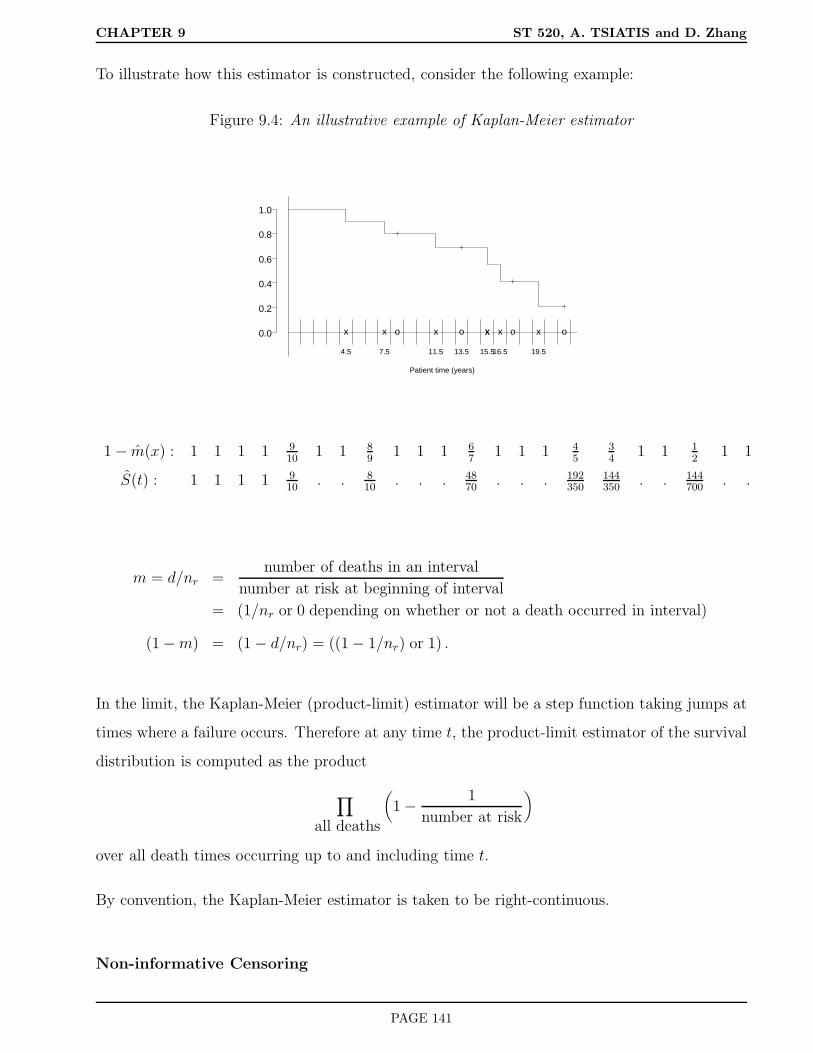
CHAPTER 9 ST 520, A. TSIATIS and D. Zhang
To illustrate how this estimator is constructed, consider the following example:
Figure 9.4: An illustrative example of Kaplan-Meier estimator
0.0
0.2
0.4
0.6
0.8
1.0
x
4.5
x
7.5
o x
11.5
o x
13.5
x
15.5
x
16.5
o x
19.5
o
Patient time (years)
1 − m(x) : 1 1 1 1 910
1 1 89
1 1 1 67
1 1 1 45
34
1 1 12
1 1
S(t) : 1 1 1 1 910
. . 810
. . . 4870
. . . 192350
144350
. . 144700
. .
m = d/nr =number of deaths in an interval
number at risk at beginning of interval
= (1/nr or 0 depending on whether or not a death occurred in interval)
(1 −m) = (1 − d/nr) = ((1 − 1/nr) or 1) .
In the limit, the Kaplan-Meier (product-limit) estimator will be a step function taking jumps at
times where a failure occurs. Therefore at any time t, the product-limit estimator of the survival
distribution is computed as the product
∏
all deaths
(1 − 1
number at risk
)
over all death times occurring up to and including time t.
By convention, the Kaplan-Meier estimator is taken to be right-continuous.
Non-informative Censoring
PAGE 141

CHAPTER 9 ST 520, A. TSIATIS and D. Zhang
In order that life-table estimators give unbiased results, there is an implicit assumption that
individuals who are censored have the same risk of subsequent failure as those who are alive and
uncensored. The risk set at any point in time (individuals still alive and uncensored) should
be representative of the entire population alive at the same time in order that the estimated
mortality rates reflect the true population mortality rates.
Some notation and software
In describing censored survival data, it is useful to conceptualize two latent random variables
(possibly unobserved) corresponding to the failure time and censoring time. For the i-th individ-
ual we will denote these by Ti and Ci respectively. Specifically, Ti represents the survival time
if that individual was followed until death; whereas, Ci corresponds to the time measured from
their entry into the study until they were censored in the hypothetical situation that they could
not die. For example, Ci may be the time from entry into the study until the time the final
analysis was conducted. However, if the individual could be lost to follow-up, then the variable
Ci would have to account for that possibility as well. In any case, Ci corresponds to the time
that an individual would have been censored in a study if their death could be prevented.
In contrast to these latent variables, the variables we actually get to observe for the i-th individual
are denoted by (Ui,∆i), where Ui denotes the observed time on study (i.e. the time to death or
censoring, and ∆i denotes the failure indicator taking on the value 1 if the patient is observed
to die and the value 0 if the patient is censored. In terms of the latent variables we assume
Ui = min(Ti, Ci) and ∆i = I(Ti ≤ Ci).
The main objective of a clinical trial is to make inference about the probability distribution of the
latent survival time Ti even though this variable is not always observed due to censoring. In the
one-sample problem we are interested in estimating the survival distribution S(t) = P (Ti ≥ t)
using a sample of observable data
(Ui,∆i), i = 1, . . . , n.
If we define the number of individuals at risk at any time t by
n(t) =n∑
i=1
I(Ui ≥ t),
that is, the number of individuals in our sample who neither died or were censored by time t,
PAGE 142

CHAPTER 9 ST 520, A. TSIATIS and D. Zhang
then the Kaplan-Meier estimator is given by
KM(t) =∏
i:Ui≤t
n(Ui) − 1
n(Ui)
∆i
.
This is the Kaplan-Meier estimator when there are no tied survival times in our sample. More
generally, if we denote by
d(t) =n∑
i=1
I(Ui = t,∆i = 1),
the number of observed deaths in our sample at time t, thus allowing the possibility that d(t) ≥ 2
in cases where survival times are tied, then we can write the Kaplan-Meier estimator as
KM(t) =∏
death times u≤t
1 − d(u)
n(u)
.
The standard error of the Kaplan-Meier estimator is also taken as the limit in Greenwood’s
formula, Namely,
seKM(t) = KM(t)
∑
death times u≤t
d(u)
n(u)n(u) − d(u)
1/2
.
Proc lifetest in SAS
Many statistical packages, including SAS, have software available for censored survival analysis.
For example, the above Kaplan-Meier estimator can be obtained using the following SAS program:
Data example;input survtime censcode;cards;4.5 17.5 18.5 011.5 113.5 015.5 116.5 117.5 019.5 121.5 0
;
Proc lifetest;time survtime*censcode(0);
run;
And part of the output from the above program is
PAGE 143

CHAPTER 9 ST 520, A. TSIATIS and D. Zhang
The LIFETEST Procedure
Product-Limit Survival Estimates
SurvivalStandard Number Number
SURVTIME Survival Failure Error Failed Left
0.0000 1.0000 0 0 0 104.5000 0.9000 0.1000 0.0949 1 97.5000 0.8000 0.2000 0.1265 2 88.5000* . . . 2 711.5000 0.6857 0.3143 0.1515 3 613.5000* . . . 3 515.5000 0.5486 0.4514 0.1724 4 416.5000 0.4114 0.5886 0.1756 5 317.5000* . . . 5 219.5000 0.2057 0.7943 0.1699 6 121.5000* . . . 6 0
* Censored Observation
9.4 Two-sample Tests
The major objective of many Phase III clinical trials is to compare two or more treatments with
respect to some primary endpoint. If the primary endpoint is time to an event (e.g. survival
time), then interest will focus on whether one treatment will increase or decrease the distribution
of this time as compared to some standard or control treatment. Let us begin by considering the
comparison of two treatments. Let the variable A denote treatment group, where we take A = 0
to denote the control group or standard treatment and A = 1 the new treatment.
The problem of comparing two treatments is often cast as a hypothesis testing question. The null
hypothesis being that the distribution of time to death (event) is the same for both treatments.
Letting T denote a patient’s underlying survival time, we define the treatment specific survival
distributions by S1(t) = P (T ≥ t|A = 1) and S0(t) = P (T ≥ t|A = 0). The null hypothesis is
given as
H0 : S1(t) = S0(t) = S(t), t > 0,
or equivalently
H0 : λ1(t) = λ0(t) = λ(t),
where λj(t), j = 0, 1 denote the treatment-specific hazard rates.
PAGE 144
CHAPTER 9 ST 520, A. TSIATIS and D. Zhang
The alternative hypothesis of most interest in such trials is that the survival time for one treat-
ment is stochastically larger than the survival time for the other treatment. Specifically, we say
the survival time for treatment 1 is stochastically larger than the survival time for treatment 0
if S1(t) ≥ S0(t) for all t > 0 with strict inequality for at least one value of t.
It has become standard practice in clinical trials to use nonparametric tests; that is, tests based
on statistics whose distribution under the null hypothesis does not depend on the underlying
survival distribution S(t) (At least asymptotically). The most widely used test with censored
survival data is the logrank test which we now describe.
Data from a clinical trial comparing the survival distribution between two treatments can be
viewed as realizations of the random triplets
(Ui,∆i, Ai), i = 1, . . . , n,
where
• Ui = min(Ti, Ci)
– Ti denotes the latent failure time
– Ci denotes the latent censoring time
• ∆i = I(Ti ≤ Ci) denotes failure indicator
• Ai denotes treatment indicator
We also define the following notation:
• nj =∑n
i=1 I(Ai = j) denotes the number of patients assigned treatment j = 0, 1; n = n0+n1
• nj(u) =∑n
i=1 I(Ui ≥ u,Ai = j) denotes the number at risk at time u from treatment
j = 0, 1
• n(u) = n0(u) + n1(u) denotes the total number at risk at time u from both treatments
• dj(u) =∑n
i=1 I(Ui = u,∆i = 1, Ai = j) denotes the number of observed deaths at time u
from treatment j = 0, 1
PAGE 145

CHAPTER 9 ST 520, A. TSIATIS and D. Zhang
• d(u) = d0(u) + d1(u) denotes the number of observed deaths at time u from both samples
The notation above allows the possibility of more than one death occurring at the same time
(tied survival times).
The logrank test is based on the statistic
∑
all death times u
d1(u) −
n1(u)
n(u)d(u)
.
This statistic can be viewed as the sum over the distinct death times of the observed number
of deaths from treatment 1 minus the expected number of deaths from treatment 1 if the null
hypothesis were true.
Thus at any point in time u corresponding to a time where a death was observed, i.e. d(u) ≥ 1,
the data at that point in time can be viewed as a 2 × 2 table; namely,
treatment
1 0 total
number of deaths d1(u) d0(u) d(u)
number alive n1(u) − d1(u) n0(u) − d0(u) n(u) − d(u)
number at risk n1(u) n0(u) n(u)
• The observed number of deaths at time u from treatment 1 is d1(u)
• The expected number of deaths from treatment 1 at time u if the null hypothesis were true
is d(u)n(u)
n1(u)
• Thus the observed minus expected number of deaths at time u isd1(u) − d(u)
n(u)n1(u)
From this point of view, the survival data from a clinical trial can be summarized as k 2 × 2
tables, where k denotes the number of distinct death times. If the null hypothesis is true, then we
would expectd1(u) − d(u)
n(u)n1(u)
to be about zero on average for all u : d(u) ≥ 1. However, if
the hazard rate for treatment 0 is greater than the hazard rate for treatment 1 consistently over
all u, then, on average, we would expectd1(u) − d(u)
n(u)n1(u)
to be negative. The opposite would
be expected if the hazard rate for treatment 1 was greater than the hazard rate for treatment 0
for all u.
PAGE 146

CHAPTER 9 ST 520, A. TSIATIS and D. Zhang
This suggests that the null hypothesis of treatment equality should be rejected if the test statistic
is sufficiently large or small depending on the alternative of interest for one-sided tests or if the
absolute value of the test statistic is sufficiently large for two-sided tests. In order to gauge the
strength of evidence against the null hypothesis we must be able to evaluate the distribution of
the test statistic (at least approximately) under the null hypothesis. Therefore, the test statistic
has to be standardized appropriately. Specifically, the logrank test is given by
Tn =
∑d1(u) − d(u)
n(u)n1(u)
[∑ n1(u)n0(u)d(u)n(u)−d(u)n2(u)n(u)−1
]1/2. (9.1)
Remark: In a 2 × 2 contingency table
d1(u) · d(u)
· · n(u) − d(u)
n1(u) n0(u) n(u)
The value d1(u), under the null hypothesis, conditional on the marginal totals, has a hypergeo-
metric distribution with meand(u)
n(u)n1(u)
and variance [∑ n1(u)n0(u)d(u)n(u) − d(u)n2(u)n(u) − 1
].
The sum of the hypergeometric variances of these 2 × 2 tables, summed over the distinct death
times, is the estimator of the variance of the test statistic under the null hypothesis. Therefore,
the logrank test Tn given by (9.1) is distributed as a standard normal under H0; i.e.
TnH0∼ N(0, 1).
Consequently, a level α test (two-sided) would reject the null hypothesis when |Tn| ≥ Zα/2. One
sided level α tests would reject whenever Tn ≥ Zα or −Tn ≥ Zα depending on the question. For
example, if we were interested in showing that treatment 1 is better (longer survival times) than
treatment 0, then we would reject H0 when −Tn ≥ Zα because under the alternative hypothesis
we would expect the observed number of deaths from treatment 1 to be less than that expected
under the null hypothesis.
PAGE 147

CHAPTER 9 ST 520, A. TSIATIS and D. Zhang
Note: All the arguments made above were based on summarizing the data as 2 × 2 tables
at distinct death times. Nowhere did we have to make any assumptions (other than the null
hypothesis) about the actual shape of the underlying survival distribution in deriving the nu-
merator of the logrank test statistic or its variance. This, intuitively, explains why this test is
nonparametric.
If censored survival data are organized as (Ui,∆i, Ai), i = 1, . . . , n, where Ui denotes time to
failure or censoring, ∆i denotes failure indicator, and Ai denotes treatment indicator, then the
logrank test can be computed using SAS. To illustrate, we again use the data from CALGB 8541
(clinical trial on beast cancer).
Recall that CALGB 8541 was a randomized three arm clinical trial for patients with stage II node
positive breast cancer. Although there were three treatments, the major focus was comparing
treatment 1 (Intensive CAF) to treatment 2 (Low dose CAF), where CAF is the combination of
the drugs Cyclophosphamide, Adriamycin an 5 Fluorouracil. For the purpose of this illustration
we will restrict attention to the comparison of these two treatments. Later we will discuss the
comparison of all three treatments.
data trt12; set bcancer;if (trt=1) or (trt=2);
run;
title "Log-rank test comparing treatments 1 and 2";proc lifetest data=trt12 notable;
time years*censor(0);strata trt;
run;
Part of the output from the above SAS program:
The LIFETEST Procedure
Testing Homogeneity of Survival Curves for years over Strata
Rank Statistics
trt Log-Rank Wilcoxon
1 -30.030 -236952 30.030 23695
PAGE 148
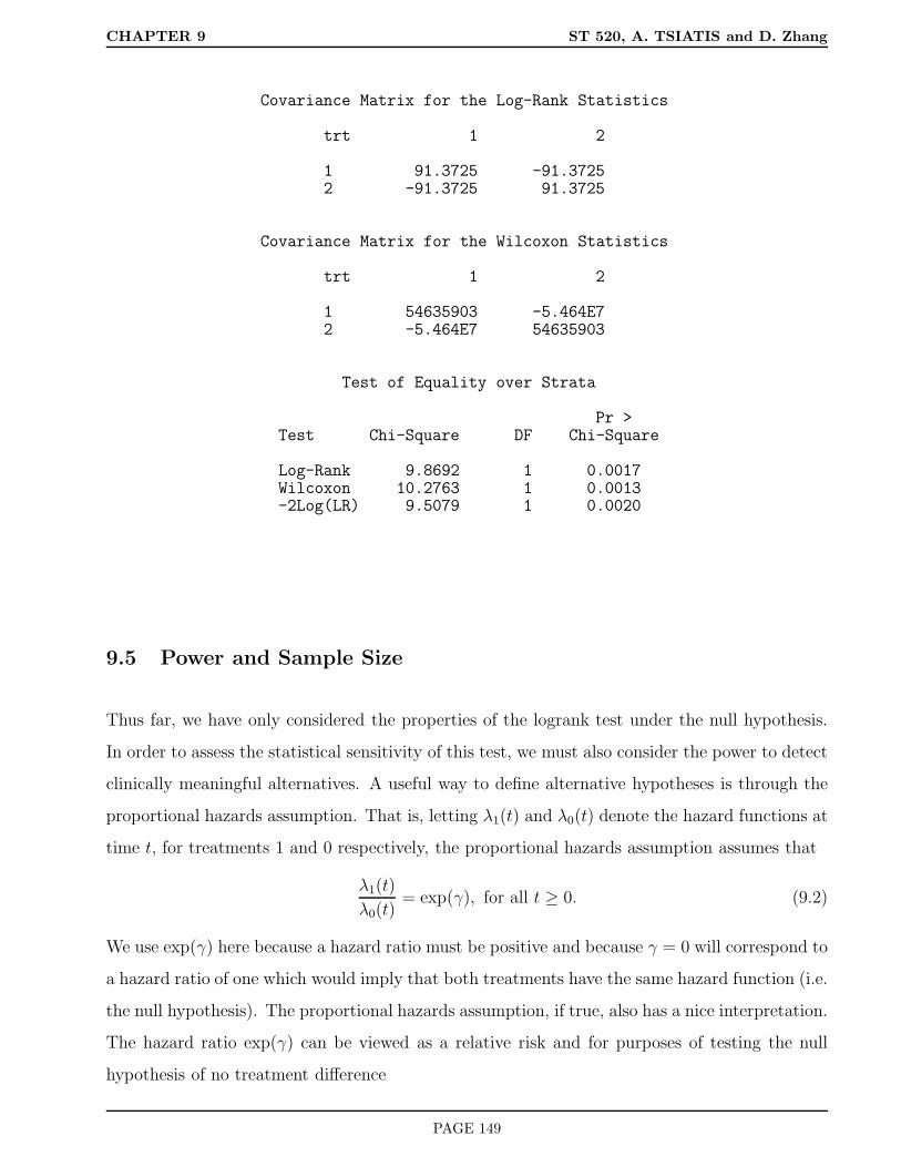
CHAPTER 9 ST 520, A. TSIATIS and D. Zhang
Covariance Matrix for the Log-Rank Statistics
trt 1 2
1 91.3725 -91.37252 -91.3725 91.3725
Covariance Matrix for the Wilcoxon Statistics
trt 1 2
1 54635903 -5.464E72 -5.464E7 54635903
Test of Equality over Strata
Pr >Test Chi-Square DF Chi-Square
Log-Rank 9.8692 1 0.0017Wilcoxon 10.2763 1 0.0013-2Log(LR) 9.5079 1 0.0020
9.5 Power and Sample Size
Thus far, we have only considered the properties of the logrank test under the null hypothesis.
In order to assess the statistical sensitivity of this test, we must also consider the power to detect
clinically meaningful alternatives. A useful way to define alternative hypotheses is through the
proportional hazards assumption. That is, letting λ1(t) and λ0(t) denote the hazard functions at
time t, for treatments 1 and 0 respectively, the proportional hazards assumption assumes that
λ1(t)
λ0(t)= exp(γ), for all t ≥ 0. (9.2)
We use exp(γ) here because a hazard ratio must be positive and because γ = 0 will correspond to
a hazard ratio of one which would imply that both treatments have the same hazard function (i.e.
the null hypothesis). The proportional hazards assumption, if true, also has a nice interpretation.
The hazard ratio exp(γ) can be viewed as a relative risk and for purposes of testing the null
hypothesis of no treatment difference
PAGE 149
CHAPTER 9 ST 520, A. TSIATIS and D. Zhang
• γ > 0 implies that individuals on treatment 1 have worse survival (i.e. die faster)
• γ = 0 implies the null hypothesis
• γ < 0 implies that individuals on treatment 1 have better survival (i.e. live longer)
If the proportional hazards assumption were true; that is,
λ1(t) = λ0(t) exp(γ),
then this would imply that
−d log S1(t)
dt= −d log S0(t)
dtexp(γ),
or
− log S1(t) = − log S0(t) exp(γ).
Consequently,
S1(t) = S0(t)exp(γ),
and
log− logS1(t) = log− logS0(t) + γ.
This last relationship can be useful if we want to assess whether a proportional hazards as-
sumption is a reasonable representation of the data. By plotting the two treatment-specific
Kaplan-Meier curves on a log− log scale we can visually inspect whether these two curves
differ from each other by a constant over time.
Also, in the special case where we feel comfortable in assuming that the survival distributions
follow an exponential distribution; i.e. constant hazards, the proportional hazards assumption is
guaranteed to hold. That is,λ1(t)
λ0(t)=λ1
λ0.
In section 9.1 we showed that the median survival time for an exponential distribution with
hazard λ is equal to m = log(2)/λ. Therefore, the ratio of the median survival times for two
treatments whose survival distributions are exponentially distributed with hazard rates λ1 and
λ0 ism1
m0
=log(2)/λ1log(2)/λ0
=λ0
λ1
.
PAGE 150
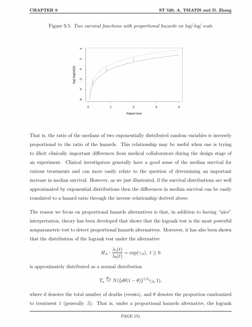
CHAPTER 9 ST 520, A. TSIATIS and D. Zhang
Figure 9.5: Two survival functions with proportional hazards on log[-log] scale
Patient time
log(
-log(
(s(t
)))
0 1 2 3 4
-6-4
-20
24
That is, the ratio of the medians of two exponentially distributed random variables is inversely
proportional to the ratio of the hazards. This relationship may be useful when one is trying
to illicit clinically important differences from medical collaborators during the design stage of
an experiment. Clinical investigators generally have a good sense of the median survival for
various treatments and can more easily relate to the question of determining an important
increase in median survival. However, as we just illustrated, if the survival distributions are well
approximated by exponential distributions then the differences in median survival can be easily
translated to a hazard ratio through the inverse relationship derived above.
The reason we focus on proportional hazards alternatives is that, in addition to having “nice”
interpretation, theory has been developed that shows that the logrank test is the most powerful
nonparametric test to detect proportional hazards alternatives. Moreover, it has also been shown
that the distribution of the logrank test under the alternative
HA :λ1(t)
λ0(t)= exp(γA), t ≥ 0
is approximately distributed as a normal distribution
TnHA∼ N(dθ(1 − θ)1/2γA, 1),
where d denotes the total number of deaths (events), and θ denotes the proportion randomized
to treatment 1 (generally .5). That is, under a proportional hazards alternative, the logrank
PAGE 151

CHAPTER 9 ST 520, A. TSIATIS and D. Zhang
test is distributed approximately as a normal random variable with variance 1 and noncentrality
parameter
dθ(1 − θ)1/2γA.
When θ = .5, the noncentrality parameter is
γAd1/2/2.
In order that a level α test (say, two-sided) have power 1 − β to detect the alternative
λ1(t)
λ0(t)= exp(γA),
then the noncentrality parameter must equal Zα/2 + Zβ . That is,
γAd1/2/2 = Zα/2 + Zβ,
or
d =4(Zα/2 + Zβ)2
γ2A
. (9.3)
This means that the power of the logrank test to detect a proportional hazards alternative is
directly related to the number of events (deaths) d during the course of the clinical trial.
Remark: This very nice and simple relationship would not apply if we didn’t use the logrank
test in conjunction with a proportional hazards alternative.
If we take α = .05 (two-sided), power (1 − β) = .90, and θ = .5, then
d =4(1.96 + 1.28)2
γ2A
. (9.4)
Some examples of the number of deaths necessary to detect an alternative where the hazard ratio
equals exp(γA) with 90% power using the logrank test at the .05 (two-sided) level of significance
is given in the following table.
Hazard Ratio exp(γA) Number of deaths d
2.00 88
1.50 256
1.25 844
1.10 4623
PAGE 152

CHAPTER 9 ST 520, A. TSIATIS and D. Zhang
During the design stage we must ensure that a sufficient number of patients are entered into the
trial and followed long enough so that the requisite number of events are attained.
Sample Size Considerations
One straightforward approach to ensure the desired power of a trial to detect a clinically impor-
tant alternative is to continue a clinical trial until we obtain the required number of failures.
Example: Suppose patients with advanced lung cancer historically have a median survival of
six months and the survival distribution is approximately exponentially distributed. An increase
in the median survival from six months to nine months is considered clinically important and
we would like to have at least 90% power to detect such a difference if it can be achieved with
a new therapy using a logrank test at the .05 (two-sided) level of significance. How should we
design a clinical trial comparing the standard treatment to a promising new treatment?
If the survival distributions for both treatments were exponentially distributed, then the clinically
important hazard ratio would be
λ1
λ0
=m0
m1
=6
9= 2/3.
Hence γA = log(2/3) = −.4055. Using the formula given by equation (9.4) we determine that
we need to carry out a study that will ultimately require a total of 256 deaths.
Since, for this example, patients do not survive for very long, one strategy is to enter some number
of patients greater than 256 and continue the study until 256 deaths occur. For example, we
may enter, say 350 patients, whom we randomize with equal probability to the two treatments
and then analyze the data after 256 deaths.
Note The 350 patients was chosen arbitrarily. We now give more careful consideration to some
of the design aspects of a clinical trial with a survival endpoint.
Design Specifications
In most clinical trials, arbitrarily picking a number of patients and waiting for the requisite
number of events to occur will not be adequate for the proper planning of the trial. More often
we need to consider the following in the proper design of a clinical trial with a time to event
endpoint.
PAGE 153

CHAPTER 9 ST 520, A. TSIATIS and D. Zhang
• number of patients
• accrual period
• follow-up time
It was shown by Schoenfeld that to obtain reasonable approximations for the power, we need the
expected number of events (deaths), computed under the alternative, to equal the number given
by equation (9.3). Specifically, the expected number of deaths need to be computed separately
for each treatment arm, under the assumption that the alternative hypothesis were true, and the
sum from both treatments should equal (9.3) to achieve the desired power.
In order to compute the expected number of deaths for each treatment during the design stage,
we must consider the following. Also, see figure below.
Figure 9.6: Illustration of accrual and follow-up
0-
Ei(Accrual) (Follow-up)
A L = A+ F
Remark: We will assume that any censoring that may occur is due to end of study censoring
resulting from staggered entry. We will sometimes refer to this as “administrative censoring”.
If, in addition, we wanted to consider other forms of censoring, such as lost to follow-up due to
withdrawal or censoring due to death from other causes, then the formulas given below would
have to be modified.
We define the following notation:
• A denotes the accrual period; that is, the calendar period of time that patients are entering
the study
• F denotes the calendar period of time after accrual has ended before the final analysis is
conducted
• L = A + F denotes the total calendar time of the study from the time the study opens
until the final analysis
PAGE 154

CHAPTER 9 ST 520, A. TSIATIS and D. Zhang
• Denote the accrual rate at calendar time u by a(u); more precisely as
a(u) = limh→0
Expected no. of patients entering between [u, u+ h)
h
.
The total expected number of patients in the clinical trial is given by
∫ A
0a(u)du.
If we have a constant accrual rate (this is the most common assumption made during the design
stage), then a(u) = a and the expected number of patients is aA.
In a randomized study where patients are assigned with equal probability to each of two treat-
ments the accrual rate to each treatment would be a(u)2
. If we denote the distribution function
of the survival time for each treatment (0 or 1) by
Fj(u) = P (T ≤ u|A = j) = 1 − Sj(u), j = 0, 1,
then the expected number of observed deaths from treatment j is
dj =∫ A
0
a(u)
2Fj(L− u)du, j = 0, 1. (9.5)
In words, we expect a(u)2du patients to enter between times [u, u+ du), of which the proportion
Fj(L − u) are expected to die by the end of the study (at time L). This number summed
(integrated) over u, for values of u during the accrual period [0, A], will yield the expected
number of deaths on treatment j = 0, 1. To get the desired power we want
d1 + d0 =4(Zα/2 + Zβ)2
γ2A
,
Note: The number of failures can be affected by
• the accrual rate
• accrual period (sample size)
• follow-up period
• the failure (hazard) rate (survival distribution)
PAGE 155

CHAPTER 9 ST 520, A. TSIATIS and D. Zhang
Some, or all, of these factors can be controlled by the investigator and have to be considered
during the design stage.
Example:
Assume the accrual rate is constant a patients per year and we randomize equally to two treat-
ments so that the accrual rate is a/2 patients per year on each treatment. Also assume that the
treatment specific survival distributions are exponentially distributed with hazards λj, j = 0, 1.
Then
dj =∫ A
0
a
2[1 − exp−λj(L− u)] du
=a
2
[A− exp(−λjL)
λjexp(λjA) − 1
].
During the design stage, we expect 100 patients per year to be recruited into the study. The
median survival for treatment 0 is expected to be about 4 years and assumed to follow an
exponential distribution (λ0 = .173). We want the power to be 90% if the new treatment
(treatment 1) can increase the median survival to 6 years (λ1 = .116) using a logrank test at the
.05 (two-sided) level of significance.
For this problem the clinically important hazard ratio is 2/3 corresponding to γA = log(2/3).
Using equation (9.3), the total number of deaths necessary is 256. Hence, we need
d1(A,L) + d0(A,L) = 256.
Note: We use the notation d1(A,L) to emphasize the fact that the number of deaths will depend
on our choice of accrual period A and length of study L.
According to the formulas we derived, we need A and L to satisfy the equation
50
[A− exp(−.116L)
.116exp(.116A) − 1
]
+50
[A− exp(−.173L)
.173exp(.173A) − 1
]
= 256.
There are many combinations of A and L that would satisfy the equation above. Clearly, the
minimum length of the study would occur if we continued accruing patients continuously until
PAGE 156

CHAPTER 9 ST 520, A. TSIATIS and D. Zhang
we obtained the desired number of events. This corresponds to the case where A = L. When
A = L there is only one unknown above and solving the equation above yields A = L = 7 years.
Such a design would require a total of 700 patients.
Note: This equation does not have a closed form solution and the solution must be obtained
numerically by iterative techniques.
In contrast, if we accrued for five years, A = 5, or a total of 500 patients, then solving for L
yields L = 7.65.
Clearly, to obtain 256 deaths, we need to accrue at least 256 patients. Therefore, A must be
greater than 2.56 years. However, choosing L that small in order to accrue as few patients as
possible would result in a trial that would take an exceedingly long time to complete.
A good strategy is to experiment with a variety of combinations of A and L that can be used to
present to the clinical investigators and then the choice which best suits the needs of the study
can be made.
Other factors that may affect power that we will not discuss are
• loss to follow-up (withdrawal)
• competing risks
• non-compliance
An excellent account on how to deal with these issues during the design stage is given by Lakatos
(1988), Biometrics.
9.6 K-Sample Tests
We now consider the case where we randomize to K > 2 treatments and are interested in testing
the null hypothesis that the survival distributions are the same for all treatments versus the
alternative that there is some difference. With right censoring, the data from such a clinical trial
can be represented as realizations of the iid triplets (Ui,∆i, Ai), i = 1, . . . , n, where for the i-th
PAGE 157

CHAPTER 9 ST 520, A. TSIATIS and D. Zhang
individual, Ui = min(Ti, Ci), ∆i = I(Ti ≤ Ci), and Ai = (1, . . . , K) denotes the treatment group
that the individual was randomized to. Letting Sj(t) = P (T ≥ t|A = j), j = 1, . . . , K denote
the treatment-specific survival distributions, the null hypothesis of no treatment difference is
H0 : S1(t) = . . . = SK(t), t ≥ 0,
or equivalently
H0 : λ1(t) = . . . = λK(t), t ≥ 0,
where λj(t), j = 1, . . . , K denote the treatment-specific hazard rates.
The test of the null hypothesis for this K-sample problem will be a direct generalization of the
logrank test used for the two-sample test. Using the same notation as in the previous section
where nj(u) denotes the number of individuals at risk at time u in treatment group j and dj(u)
the number of observed deaths in treatment group j at time u, we view the data as a series of
2 ×K tables at the distinct failure times u where d(u) ≥ 1. For example,
Treatments
1 2 . . . K Total
No. of deaths d1(u) d2(u) . . . dK(u) d(u)
No. alive n1(u) − d1(u) n2(u) − d2(u) . . . nK(u) − dK(u) n(u) − d(u)
No. at risk n1(u) n2(u) . . . nK(u) n(u)
Generalization of the two-sample test
At each time u where d(u) ≥ 1, we now consider a vector of observed minus expected number of
deaths under the null hypothesis for each treatment group j. Namely,
d1(u) − n1(u)n(u)
d(u)
···
dK(u) − nK(u)n(u)
d(u)
K×1
Note: The sum of the elements in this vector is equal to zero. Because of this, such vectors
can only vary in (K − 1)-dimensional space. Consequently, it suffices to use only K − 1 of these
PAGE 158

CHAPTER 9 ST 520, A. TSIATIS and D. Zhang
vectors for further consideration in constructing test statistics. It doesn’t matter which K − 1
of these we use, thus, for convention, we will take from now on j = 1, . . . , K − 1.
Analogous to the two-sample problem, if we condition on the marginal counts of these 2×K con-
tingency tables, then, under the null hypothesis, the distribution of the counts d1(u), . . . , dK(u)is a multivariate version of the hypergeometric distribution. Specifically, this implies that, con-
ditional on the marginal counts, the conditional expectation of dj(u) is
ECdj(u) =nj(u)
n(u)d(u), j = 1, . . . , K.
Note: We use the notation EC(·) to denote conditional expectation.
Also the conditional variance-covariance matrix of the dj(u)’s is given by
varCdj(u) =d(u)n(u) − d(u)nj(u)n(u) − nj(u)
n2(u)n(u) − 1 , j = 1, . . . , K,
and for j 6= j′
covCdj(u), dj′(u) = −[d(u)n(u) − d(u)nj(u)nj′(u)
n2(u)n(u) − 1
].
Again, analogous to the construction of the logrank test in two-samples, consider the K − 1
dimensional vector Tn, made up by the sum of the observed minus expected counts for treatments
j = 1, . . . , K − 1, summed over distinct death times u such that d(u) ≥ 1. That is
Tn =
∑death times u
d1(u) − n1(u)
n(u)d(u)
···
∑death times u
dK−1(u) − nK−1(u)
n(u)d(u)
(K−1)×1
The corresponding (K−1)×(K−1) covariance matrix of the vector Tn is given by V(K−1)×(K−1)n ,
where for j = 1, . . . , K − 1 the diagonal terms are given by
Vnjj =∑
death times u
[d(u)n(u) − d(u)nj(u)n(u) − nj(u)
n2(u)n(u) − 1
],
and for j 6= j′, the off-diagonal terms are
Vnjj′ = −∑
death times u
[d(u)n(u) − d(u)nj(u)nj′(u)
n2(u)n(u) − 1
].
PAGE 159

CHAPTER 9 ST 520, A. TSIATIS and D. Zhang
The test statistic used to test the null hypothesis is given by the quadratic form
Tn = T Tn [Vn]−1Tn,
where we use the notation (·)T to denote the transpose of a vector. Under H0, the statistic Tn
is distributed asymptotically as a central chi-square distribution with K − 1 degrees of freedom.
This test statistic is called the K-sample logrank test statistic. If the null hypothesis is true,
we would expect the elements in the vector Tn to be near zero. Hence the quadratic form, Tn,
should also be near zero. If however, there were treatment differences, then we would expect
some of the elements in the vector Tn to deviate from zero and thus expect the quadratic form,
Tn, to be larger. Thus, we will reject the null hypothesis if Tn is sufficiently large. For a level α
test, we would reject H0 when
Tn = T Tn [Vn]−1Tn ≥ χ2
α,K−1.
Proc lifetest in SAS implements this test and we will illustrate shortly using the data from
CALGB 8541. But first let us end this section with a short discussion on how sample size
calculations can be implemented during the design stage when one is comparing the survival
distribution of more than two treatments with the logrank test.
9.7 Sample-size considerations for the K-sample logrank test
The computations of the sample size necessary to attain the desired power to detect clinically
important treatment differences using the logrank test generalize from the two-sample problem to
the K-sample problem in a manner similar to that considered for the comparison of proportions
or means discussed in Chapter 7.
Specifically, if we randomize with equal probability to K treatments, then the total number of
deaths necessary for the K-sample logrank test at the α level of significance to have power at
least 1 − β to detect a hazard ratio (assumed constant over time) between any two treatments
greater than equal to exp(γA) is given by
d =2Kφ2(α, β,K − 1)
γ2A
,
where
φ2(α, β,K − 1),
PAGE 160

CHAPTER 9 ST 520, A. TSIATIS and D. Zhang
is the value of the non-centrality parameter necessary so that a non-central chi-square distributed
random variable with K − 1 degrees of freedom and non-centrality parameter φ2(α, β,K − 1)
will exceed the value χ2α;K−1 with probability (1− β). Tables of φ2(α, β,K − 1) for α = .05 were
provided in chapter 7.
For example, if we take K = 3, then in order to ensure that we have at least 90% power to detect
a hazard ratio between any two treatments that may exceed 1.5, using a logrank test at the .05
level of significance, we would need the total number of deaths to exceed
d =2 × 3 × 12.654
log(1.5)2= 462.
We can contrast this to a two-sample comparison which needs 256 events. As in the two-sample
problem, the computations during the design stage will involve the best guesses for the accrual
rate, accrual period, follow-up period, and underlying treatment-specific survival distributions
which can be translated to the desired number of failures. Thus we can experiment with different
values of
• accrual rate a(u)
• underlying treatment-specific failure time distributions Fj(t) = P (T ≤ t|A = j) = 1 −Sj(t), j = 1, . . . , K under the alternative hypothesis of interest (we may take these at the
least favorable configuration)
• the accrual period A
• the length of study L
so thatK∑
j=1
dja(·), Fj(·), A, L =2Kφ2(α, β,K − 1)
γ2A
,
where dja(·), Fj(·), A, L denotes the expected number of deaths in treatment group j as a
function of a(·), Fj(·), A, L, computed using equation (9.5).
CALGB 8541 Example
We now return to the data from CALGB 8541 which compared three treatments in a randomized
study of node positive stage II breast cancer patients. The three treatments were
PAGE 161

CHAPTER 9 ST 520, A. TSIATIS and D. Zhang
• treatment 1 (Intensive CAF)
• treatment 2 (Low dose CAF)
• treatment 3 (Standard dose CAF)
where CAF denotes the combination of Cyclophosphamide, Adriamycin and 5-Fluorouracil. As
well as testing for overall differences in the three treatments, we shall also look at the three
pairwise comparisons.
SAS program:
title "Log-rank test comparing all three treatments";proc lifetest data=bcancer notable;
time years*censor(0);strata trt;
run;
Part of the output:
Log-rank test comparing all three treatments
The LIFETEST Procedure
Testing Homogeneity of Survival Curves for years over Strata
Rank Statistics
trt Log-Rank Wilcoxon
1 -21.245 -271712 37.653 431663 -16.408 -15995
Covariance Matrix for the Log-Rank Statistics
trt 1 2 3
1 120.132 -57.761 -62.3712 -57.761 114.004 -56.2433 -62.371 -56.243 118.615
Covariance Matrix for the Wilcoxon Statistics
trt 1 2 3
PAGE 162

CHAPTER 9 ST 520, A. TSIATIS and D. Zhang
1 1.6295E8 -7.94E7 -8.355E72 -7.94E7 1.5675E8 -7.734E73 -8.355E7 -7.734E7 1.6089E8
Test of Equality over Strata
Pr >Test Chi-Square DF Chi-Square
Log-Rank 12.4876 2 0.0019Wilcoxon 12.1167 2 0.0023-2Log(LR) 11.3987 2 0.0033
PAGE 163

CHAPTER 10 ST 520, A. TSIATIS and D. Zhang
10 Early Stopping of Clinical Trials
10.1 General issues in monitoring clinical trials
Up to now we have considered the design and analysis of clinical trials assuming the data would
be analyzed at only one point in time; i.e. the final analysis. However, due to ethical as well
as practical considerations, the data are monitored periodically during the course of the study
and for a variety of reasons may be stopped early. In this section we will discuss some of the
statistical issues in the design and analysis of clinical trials which allow the possibility of early
stopping. These methods fall under the general title of group-sequential methods.
Some reasons a clinical trial may be stopped early include
• Serious toxicity or adverse events
• Established benefit
• No trend of interest
• Design or logistical difficulties too serious to fix
Since there is lot invested (scientifically, emotionally, financially, etc.) in a clinical trial by
the investigators who designed or are conducting the trial, they may not be the best suited
for deciding whether the clinical trial should be stopped. It has become common practice for
most large scale phase III clinical trials to be monitored by an independent data monitoring
committee; often referred to as a Data Safety Monitoring Board (DSMB). It is the responsibility
of this board to monitor the data from a study periodically (usually two to three times a year)
and make recommendations on whether the study should be modified or stopped. The primary
responsibility of this board is to ensure the safety and well being of the patients that have enrolled
into the trial.
PAGE 164

CHAPTER 10 ST 520, A. TSIATIS and D. Zhang
The DSMB generally has members who represent the following disciplines:
• Clinical
• Laboratory
• Epidemiology
• Biostatistics
• Data Management
• Ethics
The members of the DSMB should have no conflict of interest with the study or studies they
are monitoring; e.g. no financial holdings in the company that is developing the treatments by
member or family. All the discussions of the DSMB are confidential. The charge of the DSMB
includes:
• Protocol review
• Interim reviews
– study progress
– quality of data
– safety
– efficacy and benefit
• Manuscript review
During the early stages of a clinical trial the focus is on administrative issues regarding the
conduct of the study. These include:
• Recruitment/Entry Criteria
• Baseline comparisons
PAGE 165

CHAPTER 10 ST 520, A. TSIATIS and D. Zhang
• Design assumptions and modifications
– entry criteria
– treatment dose
– sample size adjustments
– frequency of measurements
• Quality and timeliness of data collection
Later in the study, as the data mature, the analyses focus on treatment comparisons. One of
the important issues in deciding whether a study should be stopped early is whether a treatment
difference during an interim analysis is sufficiently large or small to warrant early termination.
Group-sequential methods are rules for stopping a study early based on treatment differences
that are observed during interim analyses. The term group-sequential refers to the fact that the
data are monitored sequentially at a finite number of times (calendar) where a group of new data
are collected between the interim monitoring times. Depending on the type of study, the new
data may come from new patients entering the study or additional information from patients
already in the study or a combination of both. In this chapter we will study statistical issues in
the design and analysis of such group-sequential methods. We will take a general approach to
this problem that can be applied to many different clinical trials. This approach is referred to
as Information-based design and monitoring of clinical trials.
The typical scenario where these methods can be applied is as follows:
• A study in which data are collected over calendar time, either data from new patients
entering the study or new data collected on patients already in the study
• Where the interest is in using these data to answer a research question. Often, this is posed
as a decision problem using a hypothesis testing framework. For example, testing whether
a new treatment is better than a standard treatment or not.
• The investigators or “the monitoring board” monitor the data periodically and conduct
interim analyses to assess whether there is sufficient “strong evidence” in support of the
research hypothesis to warrant early termination of the study
PAGE 166
CHAPTER 10 ST 520, A. TSIATIS and D. Zhang
• At each monitoring time, a test statistic is computed and compared to a stopping boundary.
The stopping boundary is a prespecified value computed at each time an interim analysis
may be conducted which, if exceeded by the test statistic, can be used as sufficient evidence
to stop the study. Generally, a test statistic is computed so that its distribution is well
approximated by a normal distribution. (This has certainly been the case for all the
statistics considered in the course)
• The stopping boundaries are chosen to preserve certain operating characteristics that are
desired; i.e. level and power
The methods we present are general enough to include problem where
• t-tests are used to compare the mean of continuous random variables between treatments
• proportions test for dichotomous response variables
• logrank test for censored survival data
• tests based on likelihood methods for either discrete or continuous random variables; i.e.
Score test, Likelihood ratio test, Wald tests using maximum likelihood estimators
10.2 Information based design and monitoring
The underlying structure that is assumed here is that the data are generated from a probability
model with population parameters ∆, θ, where ∆ denotes the parameter of primary interest, in
our case, this will generally be treatment difference, and θ denote the nuisance parameters. We
will focus primarily on two-sided tests where we are testing the null hypothesis
H0 : ∆ = 0
versus the alternative
HA : ∆ 6= 0,
however, the methods are general enough to also consider one-sided tests where we test
H0 : ∆ ≤ 0
PAGE 167

CHAPTER 10 ST 520, A. TSIATIS and D. Zhang
versus
HA : ∆ > 0.
Remark This is the same framework that has been used throughout the course.
At any interim analysis time t, our decision making will be based on the test statistic
T (t) =∆(t)
se∆(t),
where ∆(t) is an estimator for ∆ and se∆(t) is the estimated standard error of ∆(t) using
all the data that have accumulated up to time t. For two-sided tests we would reject the null
hypothesis if the absolute value of the test statistic |T (t)| were sufficiently large and for one-sided
tests if T (t) were sufficiently large.
Example 1. (Dichotomous response)
Let π1, π0 denote the population response rates for treatments 1 and 0 (say new treatment and
control) respectively. Let the treatment difference be given by
∆ = π1 − π0
The test of the null hypothesis will be based on
T (t) =p1(t) − p0(t)√
p(t)1 − p(t)
1n1(t)
+ 1n2(t)
,
where using all the data available through time t, pj(t) denotes the sample proportion responding
among the nj(t) individuals on treatment j = 0, 1.
Example 2. (Time to event)
Suppose we assume a proportional hazards model. Letting A denote treatment indicator, we
consider the modelλ1(t)
λ0(t)= exp(−∆),
and we want to test the null hypothesis of no treatment difference
H0 : ∆ = 0
versus the two-sided alternative
HA : ∆ 6= 0,
PAGE 168

CHAPTER 10 ST 520, A. TSIATIS and D. Zhang
or the one-sided test that treatment 1 does not improve survival
H0 : ∆ ≤ 0
versus the alternative that it does improve survival
HA : ∆ > 0.
Using all the survival data up to time t (some failures and some censored observations), we would
compute the test statistic
T (t) =∆(t)
se∆(t),
where ∆(t) is the maximum partial likelihood estimator of ∆ that was derived by D. R. Cox
and se∆(t) is the corresponding standard error. For the two-sided test we would reject the
null hypothesis if |T (t)| were sufficiently large and for the one-sided test if T (t) were sufficiently
large.
Remark: The material on the use and the properties of the maximum partial likelihood estimator
are taught in the classes on Survival Analysis. We note, however, that the logrank test computed
using all the data up to time t is equivalent asymptotically to the test based on T (t).
Example 3. (Parametric models)
Any parametric model where we assume the underlying density of the data is given by p(z; ∆, θ),
and use for ∆(t) the maximum likelihood estimator for ∆ and for se∆(t) compute the estimated
standard error using the square-root of the inverse of the observed information matrix, with the
data up to time t.
In most important applications the test statistic has the property that the distribution when
∆ = ∆∗ follows a normal distribution, namely,
T (t) =∆(t)
se∆(t)∆=∆∗
∼ N(∆∗I1/2(t,∆∗), 1),
where I(t,∆∗) denotes the statistical information at time t. Statistical information refers to
Fisher information, but for those not familiar with these ideas, for all practical purposes, we can
equate (at least approximately) information with the standard error of the estimator; namely,
I(t,∆∗) ≈ se(∆(t)−2.
PAGE 169

CHAPTER 10 ST 520, A. TSIATIS and D. Zhang
Under the null hypothesis ∆ = 0, the distribution follows a standard normal, that is
T (t)∆=0∼ N(0, 1),
and is used a basis for a group-sequential test. For instance, if we considered a two-sided test,
we would reject the null hypothesis whenever
|T (t)| ≥ b(t),
where b(t) is some critical value or what we call a boundary value. If we only conducted one
analysis and wanted to construct a test at the α level of significance, then we would choose
b(t) = Zα/2. Since under the null hypothesis the distribution of T (t) is N(0, 1) then
PH0|T (t)| ≥ Zα/2 = α.
If, however, the data were monitored at K different times, say, t1, . . . , tK , then we would want to
have the opportunity to reject the null hypothesis if the test statistic, computed at any of these
times, was sufficiently large. That is, we would want to reject H0 at the first time tj , j = 1, . . . , K
such that
|T (tj)| ≥ b(tj),
for some properly chosen set of boundary values b(t1), . . . , b(tK).
Note: In terms of probabilistic notation, using this strategy, rejecting the null hypothesis cor-
responds to the eventK⋃
j=1
|T (tj)| ≥ b(tj).
Similarly, accepting the null hypothesis corresponds to the event
K⋂
j=1
|T (tj)| < b(tj).
The crucial issue is how large should the treatment differences be during the interim analyses
before we reject H0; that is, how do we choose the boundary values b(t1), . . . , b(tK)? Moreover,
what are the consequences of such a strategy of sequential testing on the level and power of the
test and how does this affect sample size calculations?
PAGE 170

CHAPTER 10 ST 520, A. TSIATIS and D. Zhang
10.3 Type I error
We start by first considering the effect that group-sequential testing has on type I error; i.e.
on the level of the test. Some thought must be given on the choice of boundary values. For
example, since we have constructed the test statistic T (tj) to have approximately a standard
normal distribution, if the null hypothesis were true, at each time tj , if we naively reject H0
at the first monitoring time that the absolute value of the test statistic exceeds 1.96 (nominal
p-value of .05), then the type I error will be inflated due to multiple comparisons. That is,
type I error = PH0[
K⋃
j=1
|T (tj)| ≥ 1.96] > .05,
if K ≥ 2.
This is illustrated in the following table:
Table 10.1: Effect of multiple looks on type I error
K false positive rate
1 0.050
2 0.083
3 0.107
4 0.126
5 0.142
10 0.193
20 0.246
50 0.320
100 0.274
1,000 0.530
∞ 1.000
The last entry in this table was described by J. Cornfield as
“Sampling to a foregone conclusion”.
PAGE 171

CHAPTER 10 ST 520, A. TSIATIS and D. Zhang
Our first objective is to derive group-sequential tests (i.e. choice of boundaries b(t1), . . . , b(tK))
that have the desired prespecified type I error of α.
Level α test
We want the probability of rejecting H0, when H0 is true, to be equal to α, say .05. The strategy
for rejecting or accepting H0 is as follows:
• Stop and reject H0 at the first interim analysis if
|T (t1)| ≥ b(t1)
• or stop and reject H0 at the second interim analysis if
|T (t1)| < b(t1), |T (t2)| ≥ b(t2)
• or . . .
• or stop and reject at the final analysis if
|T (t1)| < b(t1), . . . , |T (tK−1)| < b(tK−1), |T (tK)| ≥ b(tK)
• otherwise, accept H0 if
|T (t1)| < b(t1), . . . , |T (tK)| < b(tK).
This representation partitions the sample space into mutually exclusive rejection regions and
an acceptance region. In order that our testing procedure have level α, the boundary values
b(t1), . . . , b(tK) must satisfy
P∆=0|T (t1)| < b(t1), . . . , |T (tK)| < b(tK) = 1 − α. (10.1)
Remark:
By construction, the test statistic T (tj) will be approximately distributed as a standard nor-
mal, if the null hypothesis is true, at each time point tj . However, to ensure that the group-
sequential test have level α, the equality given by (10.1) must be satisfied. The probability on
PAGE 172

CHAPTER 10 ST 520, A. TSIATIS and D. Zhang
the left hand side of equation (10.1) involves the joint distribution of the multivariate statistic
(T (t1), . . . , T (tK)). Therefore, we would need to know the joint distribution of this sequentially
computed test statistic at times t1, . . . , tK , under the null hypothesis, in order to compute the
necessary probabilities to ensure a level α test. Similarly, we would need to know the joint dis-
tribution of this multivariate statistic, under the alternative hypothesis to compute the power of
such a group-sequential test.
The major result which allows the use of a general methodology for monitoring clinical trials is
that
“Any efficient based test or estimator for ∆, properly normalized, when computed se-
quentially over time, has, asymptotically, a normal independent increments process
whose distribution depends only on the parameter ∆ and the statistical informa-
tion.”
Scharfstein, Tsiatis and Robins (1997). JASA. 1342-1350.
As we mentioned earlier the test statistics are constructed so that when ∆ = ∆∗
T (t) =∆(t)
se∆(t)∼ N(∆∗I1/2(t,∆∗), 1),
where we can approximate statistical information I(t,∆∗) by [se∆(t)]−2. If we normalize by
multiplying the test statistic by the square-root of the information; i.e.
W (t) = I1/2(t,∆∗)T (t),
then this normalized statistic, computed sequentially over time, will have the normal independent
increments structure alluded to earlier. Specifically, if we compute the statistic at times t1 <
t2 < . . . < tK , then the joint distribution of the multivariate vector W (t1), . . . ,W (tK) is
asymptotically normal with mean vector ∆∗I(t1,∆∗), . . . ,∆∗I(tK ,∆
∗) and covariance matrix
where
varW (tj) = I(tj ,∆∗), j = 1, . . . , K
and
cov[W (tj), W (tℓ) −W (tj)] = 0, j < ℓ, j, ℓ = 1, . . . , K.
That is
PAGE 173

CHAPTER 10 ST 520, A. TSIATIS and D. Zhang
• The statistic W (tj) has mean and variance proportional to the statistical information at
time tj
• Has independent increments; that is
W (t1) = W (t1)
W (t2) = W (t1) + W (t2) −W (t1)
·
·
·
W (tj) = W (t1) + W (t2) −W (t1) + . . .+ W (tj) −W (tj−1)
has the same distribution as a partial sum of independent normal random variables
This structure implies that the covariance matrix of W (t1), . . . ,W (tK) is given by
varW (tj) = I(tj ,∆∗), j = 1, . . . , K
and for j < ℓ
covW (tj),W (tℓ)
= cov[W (tj), W (tℓ) −W (tj) +W (tj)]
= cov[W (tj), W (tℓ) −W (tj)] + covW (tj),W (tj)
= 0 + varW (tj)
= I(tj,∆∗).
Since the test statistic
T (tj) = I−1/2(tj,∆∗)W (tj), j = 1, . . . , K
this implies that the joint distribution of T (t1), . . . , T (tK) is also multivariate normal where
the mean
ET (tj) = ∆∗I1/2(tj ,∆∗), j = 1, . . . , K (10.2)
and the covariance matrix is such that
varT (tj) = 1, j = 1, . . . , K (10.3)
PAGE 174

CHAPTER 10 ST 520, A. TSIATIS and D. Zhang
and for j < ℓ, the covariances are
covT (tj), T (tℓ) = covI−1/2(tj ,∆∗)W (tj), I
−1/2(tℓ,∆∗)W (tℓ)
= I−1/2(tj,∆∗)I−1/2(tℓ,∆
∗)covW (tj),W (tℓ)
= I−1/2(tj,∆∗)I−1/2(tℓ,∆
∗)I(tj ,∆∗)
=I1/2(tj ,∆
∗)
I1/2(tℓ,∆∗)=
√√√√I(tj,∆∗)
I(tℓ,∆∗). (10.4)
In words, the covariance of T (tj) and T (tℓ) is the square-root of the relative information at times
tj and tℓ. Hence, under the null hypothesis ∆ = 0, the sequentially computed test statistic
T (t1), . . . , T (tK) is multivariate normal with mean vector zero and covariance matrix (in this
case the same as the correlation matrix, since the variances are all equal to one)
VT =
√√√√I(tj , 0)
I(tℓ, 0)
, j ≤ ℓ. (10.5)
The importance of this result is that the joint distribution of the sequentially computed test statis-
tic, under the null hypothesis, is completely determined by the relative proportion of information
at each of the monitoring times t1, . . . , tK . This then allows us to evaluate probabilities such as
those in equation (10.1) that are necessary to find appropriate boundary values b(t1), . . . , b(tK)
that achieve the desired type I error of α.
10.3.1 Equal increments of information
Let us consider the important special case where the test statistic is computed after equal incre-
ments of information; that is
I(t1, ·) = I, I(T2, ·) = 2I, . . . , I(tK , ·) = KI.
Remark: For problems where the response of interest is instantaneous, whether this response be
discrete or continuous, the information is proportional to the number of individuals under study.
In such cases, calculating the test statistic after equal increments of information is equivalent to
calculating the statistic after equal number of patients have entered the study. So, for instance, if
we planned to accrue a total of 100 patients with the goal of comparing the response rate between
PAGE 175

CHAPTER 10 ST 520, A. TSIATIS and D. Zhang
two treatments, we may wish to monitor five times after equal increments of information; i.e after
every 20 patients enter the study.
In contrast, if we were comparing the survival distributions with possibly right censored data,
then it turns out that information is directly proportional to the number of deaths. Thus, for
such a study, monitoring after equal increments of information would correspond to conducting
interim analyses after equal number of observed deaths.
In any case, monitoring a study K times after equal increments of information imposes a
very specific distributional structure, under the null hypothesis, for the sequentially com-
puted test statistic that can be exploited in constructing group-sequential tests. Because
I(tj , 0) = jI, j = 1, . . . , K, this means that the joint distribution of the sequentially com-
puted test statistic T (t1), . . . , T (tK) is a multivariate normal with mean vector equal to zero
and by (10.5) with a covariance matrix equal to
VT =
√√√√I(tj , 0)
I(tℓ, 0)=
√j
ℓ
, j ≤ ℓ. (10.6)
This means that under the null hypothesis the joint distribution of the sequentially computed
test statistic computed after equal increments of information is completely determined once we
know the total number K of interim analyses that are intended. Now, we are in a position to
compute probabilities such as
P∆=0|T (t1)| < b1, . . . , |T (tK)| < bK
in order to determine boundary values b1, . . . , bK where the probability above equals 1 − α as
would be necessary for a level-α group-sequential test.
PAGE 176

CHAPTER 10 ST 520, A. TSIATIS and D. Zhang
Remark: The computations necessary to compute such integrals of multivariate normals with
the covariance structure (10.6) can be done quickly using using recursive numerical integration
that was first described by Armitage, McPherson and Rowe (1969). This method takes advantage
of the fact that the joint distribution is that of a standardized partial sum of independent normal
random variables. This integration allows us to search for different combinations of b1, . . . , bK
which satisfy
P∆=0|T (t1)| < b1, . . . , |T (tK)| < bK = 1 − α.
There are infinite combinations of such boundary values that lead to level-α tests; thus, we need
to assess the statistical consequences of these different combinations to aid us in making choices
in which to use.
10.4 Choice of boundaries
Let us consider the flexible class of boundaries proposed by Wang and Tsiatis (1987) Biometrics.
For the time being we will restrict attention to group-sequential tests computed after equal
increments of information and later discuss how this can be generalized. The boundaries by
Wang and Tsiatis were characterized by a power function which we will denote by Φ. Specifically,
we will consider boundaries where
bj = (constant) × j(Φ−.5), .
Different values of Φ will characterize different shapes of boundaries over time. We will also refer
to Φ as the shape parameter.
For any value Φ, we can numerically derive the the constant necessary to obtain a level-α test.
Namely, we can solve for the value c such that
P∆=0K⋂
j=1
|T (tj)| < cj(Φ−.5) = 1 − α.
Recall. Under the null hypothesis, the joint distribution of T (t1), . . . , T (tK) is completely
known if the times t1, . . . , tK are chosen at equal increments of information. The above integral
is computed for different c until we solve the above equation. That a solution exists follows from
the monotone relationship of the above probability as a function of c. The resulting solution will
be denoted by c(α,K,Φ). Some of these are given in the following table.
PAGE 177

CHAPTER 10 ST 520, A. TSIATIS and D. Zhang
Table 10.2: Group-sequential boundaries for two-sided tests for selected values of α, K, Φ
K
Φ 2 3 4 5
α = .05
0.0 2.7967 3.4712 4.0486 4.5618
0.1 2.6316 3.1444 3.5693 3.9374
0.2 2.4879 2.8639 3.1647 3.4175
0.3 2.3653 2.6300 2.8312 2.9945
0.4 2.2636 2.4400 2.5652 2.6628
0.5 2.1784 2.2896 2.3616 2.4135
α = .01
0.0 3.6494 4.4957 5.2189 5.8672
0.1 3.4149 4.0506 4.5771 5.0308
0.2 3.2071 3.6633 4.0276 4.3372
0.3 3.0296 3.3355 3.5706 3.7634
0.4 2.8848 3.0718 3.2071 3.3137
0.5 2.7728 2.8738 2.9395 2.9869
Examples: Two boundaries that have been discussed extensively in the literature and have been
used in many instances are special cases of the class of boundaries considered above. These are
when Φ = .5 and Φ = 0. The first boundary when Φ = .5 is the Pocock boundary; Pocock (1977)
Biometrika and the other when Φ = 0 is the O’Brien-Fleming boundary; O’Brien and Fleming
(1979) Biometrics.
10.4.1 Pocock boundaries
The group-sequential test using the Pocock boundaries rejects the null hypothesis at the first
interim analysis time tj , j = 1, . . . , K (remember equal increments of information) that
|T (tj)| ≥ c(α,K, 0.5), j = 1, . . . , K.
That is, the null hypothesis is rejected at the first time that the standardized test statistic using
all the accumulated data exceeds some constant.
PAGE 178

CHAPTER 10 ST 520, A. TSIATIS and D. Zhang
For example, if we take K = 5 and α = .05, then according to Table 10.2 c(.05, 5, 0.5) = 2.41.
Therefore, the .05 level test which will be computed a maximum of 5 times after equal increments
of information will reject the null hypothesis at the first time that the standardized test statistic
exceeds 2.41; that is, we reject the null hypothesis at the first time tj , j = 1, . . . , 5 when |T (tj)| ≥2.41. This is also equivalent to rejecting the null hypothesis at the first time tj , j = 1, . . . , 5 that
the nominal p-value is less than .0158.
10.4.2 O’Brien-Fleming boundaries
The O’Brien-Fleming boundaries have a shape parameter Φ = 0. A group-sequential test using
the O’Brien-Fleming boundaries will reject the null hypothesis at the first time tj, j = 1, . . . , K
when
|T (tj)| ≥ c(α,K, 0.0)/√j, j = 1, . . . , K.
For example, if we again choose K = 5 and α = .05, then according to Table 10.2 c(.05, 5, 0.0) =
4.56. Therefore, using the O’Brien-Fleming boundaries we would reject at the first time tj, j =
1, . . . , 5 when
|T (tj)| ≥ 4.56/√j, j = 1, . . . , 5.
Therefore, the five boundary values in this case would be b1 = 4.56, b2 = 3.22, b3 = 2.63,
b4 = 2.28, and b5 = 2.04
The nominal p-values for the O’Brien-Fleming boundaries are contrasted to those from the
Pocock boundaries, for K = 5 and α = .05 in the following table.
Table 10.3: Nominal p-values for K = 5 and α = .05
Nominal p-value
j Pocock O’Brien-Fleming
1 0.0158 0.000005
2 0.0158 0.00125
3 0.0158 0.00843
4 0.0158 0.0225
5 0.0158 0.0413
PAGE 179
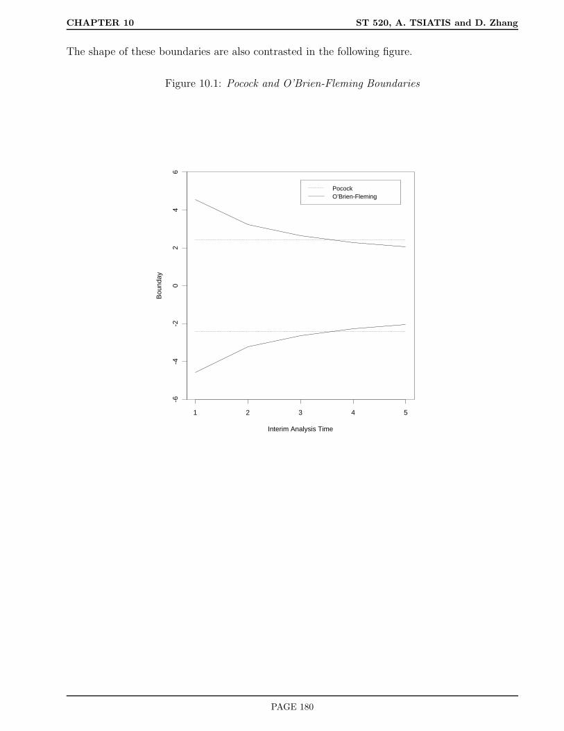
CHAPTER 10 ST 520, A. TSIATIS and D. Zhang
The shape of these boundaries are also contrasted in the following figure.
Figure 10.1: Pocock and O’Brien-Fleming Boundaries
Interim Analysis Time
Bou
nday
1 2 3 4 5
-6-4
-20
24
6
PocockO’Brien-Fleming
PAGE 180

CHAPTER 10 ST 520, A. TSIATIS and D. Zhang
10.5 Power and sample size in terms of information
We have discussed the construction of group-sequential tests that have a pre-specified level of
significance α. We also need to consider the effect that group-sequential tests have on power and
its implications on sample size. To set the stage, we first review how power and sample size are
determined with a single analysis using information based criteria.
As shown earlier, the distribution of the test statistic computed at a specific time t; namely T (t),
under the null hypothesis, is
T (t)∆=0∼ N(0, 1)
and for a clinically important alternative, say ∆ = ∆A is
T (t)∆=∆A∼ N(∆AI
1/2(t,∆A), 1),
where I(t,∆A) denotes statistical information which can be approximated by [se∆(t)]−2, and
∆AI1/2(t,∆A) is the noncentrality parameter. In order that a two-sided level-α test have power
1 − β to detect the clinically important alternative ∆A, we need the noncentrality parameter
∆AI1/2(t,∆A) = Zα/2 + Zβ,
or
I(t,∆A) =
Zα/2 + Zβ
∆A
2
. (10.7)
From this relationship we see that the power of the test is directly dependent on statistical
information. Since information is approximated by [se∆(t)]−2, this means that the study
should collect enough data to ensure that
[se∆(t)]−2 =
Zα/2 + Zβ
∆A
2
.
Therefore one strategy that would guarantee the desired power to detect a clinically important
difference is to monitor the standard error of the estimated difference through time t as data
were being collected and to conduct the one and only final analysis at time tF where
[se∆(tF )]−2 =
Zα/2 + Zβ
∆A
2
using the test which rejects the null hypothesis when
|T (tF )| ≥ Zα/2.
PAGE 181
CHAPTER 10 ST 520, A. TSIATIS and D. Zhang
Remark Notice that we didn’t have to specify any of the nuisance parameters with this
information-based approach. The accuracy of this method to achieve power depends on how
good the approximation of the distribution of the test statistic is to a normal distribution and
how good the approximation of [se∆(tF )]−2 is to the Fisher information. Some preliminary
numerical simulations have shown that this information-based approach works very well if the
sample sizes are sufficiently large as would be expected in phase III clinical trials.
In actuality, we cannot launch into a study and tell the investigators to keep collecting data until
the standard error of the estimated treatment difference is sufficiently small (information large)
without giving them some idea how many resources they need (i.e. sample size, length of study,
etc.). Generally, during the design stage, we posit some guesses of the nuisance parameters and
then use these guesses to come up with some initial design.
For example, if we were comparing the response rate between two treatments, say treatment 1
and treatment 0, and were interested in the treatment difference π1 − π0, where πj denotes the
population response probability for treatment j = 0, 1, then, at time t, we would estimate the
treatment difference using ∆(t) = p1(t) − p0(t), where pj(t) denotes the sample proportion that
respond to treatment j among the individuals assigned to treatment j by time t for j = 0, 1.
The standard error of ∆(t) = p1(t) − p0(t) is given by
se∆(t) =
√√√√π1(1 − π1)
n1(t)+π0(1 − π0)
n0(t).
Therefore, to obtain the desired power of 1 − β to detect the alternative where the population
response rates were π1 and π0, with π1 − π0 = ∆A, we would need the sample sizes n1(tF ) and
n0(tF ) to satisfy
π1(1 − π1)
n1(tF )+π0(1 − π0)
n0(tF )
−1
=
Zα/2 + Zβ
∆A
2
.
Remark: The sample size formula given above is predicated on the use of the test statistic
T (t) =p1(t) − p0(t)√
p1(t)1−p1(t)n1(t)
+ p0(t)1−p0(t)n0(t)
to test for treatment difference in the response rates. Strictly speaking, this is not the same as
the proportions test
T (t) =p1(t) − p0(t)√
p(t)1 − p(t)
1n1(t)
+ 1n0(t)
,
PAGE 182

CHAPTER 10 ST 520, A. TSIATIS and D. Zhang
although the difference between the two tests is inconsequential with equal randomization and
large samples. What we discussed above is essentially the approach taken for sample size calcu-
lations used in Chapter 6 of the notes. The important point here is that power is driven by the
amount of statistical information we have regarding the parameter of interest from the available
data. The more data the more information we have. To achieve power 1 − β to detect the
clinically important difference ∆A using a two-sided test at the α level of significance means that
we need to have collected enough data so that the statistical information equals
Zα/2 + Zβ
∆A
2
.
Let us examine how issues of power and information relate to group-sequential tests. If we are
planning to conduct K interim analyses after equal increments of information, then the power
of the group-sequential test to detect the alternative ∆ = ∆A is given by
1 − P∆=∆A|T (t1)| < b1, . . . , |T (tK)| < bK.
In order to compute probabilities of events such as that above we need to know the joint distri-
bution of the vector T (t1), . . . , T (tK) under the alternative hypothesis ∆ = ∆A.
It will be useful to consider the maximum information at the final analysis which we will denote
as MI. A K-look group-sequential test with equal increments of information and with maximum
information MI would have interim analyses conducted at times tj where j×MI/K information
has occurred; that is,
I(tj ,∆A) = j ×MI/K, j = 1, . . . , K. (10.8)
Using the results (10.2)-(10.4) and (10.8) we see that the joint distribution of T (t1), . . . , T (tK),under the alternative hypothesis ∆ = ∆A, is a multivariate normal with mean vector
∆A
√j ×MI
K, j = 1, . . . , K
and covariance matrix VT given by (10.6). If we define
δ = ∆A
√MI,
then the mean vector is equal to
(δ
√1
K, δ
√2
K, . . . , δ
√K − 1
K, δ). (10.9)
PAGE 183

CHAPTER 10 ST 520, A. TSIATIS and D. Zhang
A group-sequential level-α test from the Wang-Tsiatis family rejects the null hypothesis at the
first time tj , j = 1, . . . , K where
|T (tj)| ≥ c(α,K,Φ)j(Φ−.5).
For the alternative HA : ∆ = ∆A and maximum information MI, the power of this test is
1 − Pδ[K⋂
j=1
|T (tj)| < c(α,K,Φ)j(Φ−.5)],
where δ = ∆A
√MI, and T (t1), . . . , T (tK) is multivariate normal with mean vector (10.9) and
covariance matrix VT given by (10.6). For fixed values of α, K, and Φ, the power is an increasing
function of δ which can be computed numerically using recursive integration. Consequently, we
can solve for the value δ that gives power 1− β above. We denote this solution by δ(α,K,Φ, β).
Remark: The value δ plays a role similar to that of a noncentrality parameter.
Since δ = ∆A
√MI , this implies that a group-sequential level-α test with shape parameter Φ,
computed at equal increments of information up to a maximum of K times needs the maximum
information to equal
∆A
√MI = δ(α,K,Φ, β)
or
MI =
δ(α,K,Φ, β)
∆A
2
to have power 1 − β to detect the clinically important alternative ∆ = ∆A.
10.5.1 Inflation Factor
A useful way of thinking about the maximum information that is necessary to achieve prespecified
power with a group-sequential test is to relate this to the information necessary to achieve
prespecified power with a fixed sample design. In formula (10.7), we argued that the information
necessary to detect the alternative ∆ = ∆A with power 1 − β using a fixed sample test at level
α is
IFS =
Zα/2 + Zβ
∆A
2
.
PAGE 184

CHAPTER 10 ST 520, A. TSIATIS and D. Zhang
In contrast, the maximum information necessary at the same level and power to detect the same
alternative using a K-look group-sequential test with shape parameter Φ is
MI =
δ(α,K,Φ, β)
∆A
2
.
Therefore
MI =
Zα/2 + Zβ
∆A
2 δ(α,K,Φ, β)
Zα/2 + Zβ
2
= IFS × IF (α,K,Φ, β),
where
IF (α,K,Φ, β) =
δ(α,K,Φ, β)
Zα/2 + Zβ
2
is the inflation factor, or the relative increase in information necessary for a group-sequential test
to have the same power as a fixed sample test.
Note: The inflation factor does not depend on the endpoint of interest or the magnitude of the
treatment difference that is considered clinically important. It only depends on the level (α),
power (1− β), and the group-sequential design (K,Φ). The inflation factors has been tabulated
for some of the group-sequential tests which are given in the following table.
PAGE 185
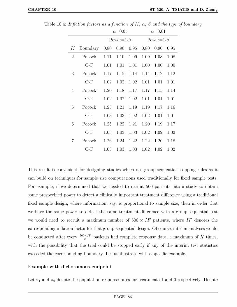
CHAPTER 10 ST 520, A. TSIATIS and D. Zhang
Table 10.4: Inflation factors as a function of K, α, β and the type of boundary
α=0.05 α=0.01
Power=1-β Power=1-β
K Boundary 0.80 0.90 0.95 0.80 0.90 0.95
2 Pocock 1.11 1.10 1.09 1.09 1.08 1.08
O-F 1.01 1.01 1.01 1.00 1.00 1.00
3 Pocock 1.17 1.15 1.14 1.14 1.12 1.12
O-F 1.02 1.02 1.02 1.01 1.01 1.01
4 Pocock 1.20 1.18 1.17 1.17 1.15 1.14
O-F 1.02 1.02 1.02 1.01 1.01 1.01
5 Pocock 1.23 1.21 1.19 1.19 1.17 1.16
O-F 1.03 1.03 1.02 1.02 1.01 1.01
6 Pocock 1.25 1.22 1.21 1.20 1.19 1.17
O-F 1.03 1.03 1.03 1.02 1.02 1.02
7 Pocock 1.26 1.24 1.22 1.22 1.20 1.18
O-F 1.03 1.03 1.03 1.02 1.02 1.02
This result is convenient for designing studies which use group-sequential stopping rules as it
can build on techniques for sample size computations used traditionally for fixed sample tests.
For example, if we determined that we needed to recruit 500 patients into a study to obtain
some prespecified power to detect a clinically important treatment difference using a traditional
fixed sample design, where information, say, is proportional to sample size, then in order that
we have the same power to detect the same treatment difference with a group-sequential test
we would need to recruit a maximum number of 500 × IF patients, where IF denotes the
corresponding inflation factor for that group-sequential design. Of course, interim analyses would
be conducted after every 500×IFK
patients had complete response data, a maximum of K times,
with the possibility that the trial could be stopped early if any of the interim test statistics
exceeded the corresponding boundary. Let us illustrate with a specific example.
Example with dichotomous endpoint
Let π1 and π0 denote the population response rates for treatments 1 and 0 respectively. Denote
PAGE 186

CHAPTER 10 ST 520, A. TSIATIS and D. Zhang
the treatment difference by ∆ = π1−π0 and consider testing the null hypothesis H0 : ∆ = 0 versus
the two-sided alternative HA : ∆ 6= 0. We decide to use a 4-look O’Brien-Fleming boundary; i.e.
K = 4 and Φ = 0, at the .05 level of significance (α = .05). Using Table 10.2, we derive the
boundaries which correspond to rejecting H0 whenever
|T (tj)| ≥ 4.049/√j, j = 1, . . . , 4.
The boundaries are given by
Table 10.5: Boundaries for a 4-look O-F test
j bj nominal p-value
1 4.05 .001
2 2.86 .004
3 2.34 .019
4 2.03 .043
In designing the trial, the investigators tell us that they expect the response rate on the control
treatment (treatment 0) to be about .30 and want to have at least 90% power to detect a
significant difference if the new treatment increases the response by .15 (i.e. from .30 to .45)
using a two-sided test at the .05 level of significance. They plan to conduct a two arm randomized
study with equal allocation and will test the null hypothesis using the standard proportions test.
The traditional fixed sample size calculations using the methods of chapter six, specifically for-
mula (6.4), results in the desired fixed sample size of
nFS =
1.96 + 1.28√
.3×.7+.45×.552×.375×.625
.15
2
× 4 × .375 × .625 = 434,
or 217 patients per treatment arm.
Using the inflation factor from Table 10.4 for the 4-look O’Brien-Fleming boundaries at the
.05 level of significance and 90% power i.e. 1.02, we compute the maximum sample size of
434 × 1.02=444, or 222 per treatment arm. To implement this design, we would monitor the
data after every 222/4 ≈ 56 individuals per treatment arm had complete data regarding their
response for a maximum of four times. At each of the four interim analyses we would compute
PAGE 187

CHAPTER 10 ST 520, A. TSIATIS and D. Zhang
the test statistic, i.e. the proportions test
T (tj) =p1(tj) − p0(tj)√
p(tj)1 − p(tj)
1n1(tj)
+ 1n0(tj )
,
using all the data accumulated up to the j-th interim analysis. If at any of the four interim anal-
yses the test statistic exceeded the corresponding boundary given in Table 10.5 or, equivalently,
if the two-sided p-value was less than the corresponding nominal p-value in Table 10.5, then we
would reject H0. If we failed to reject at all four analyses we would then accept H0.
10.5.2 Information based monitoring
In the above example it was assumed that the response rate on the control treatment arm was .30.
This was necessary for deriving sample sizes. It may be, in actuality, that the true response rate
for the control treatment is something different, but even so, if the new treatment can increase
the probability of response by .15 over the control treatment we may be interested in detecting
such a difference with 90% power. We’ve argued that power is directly related to information.
For a fixed sample design, the information necessary to detect a difference ∆ = .15 between the
response probabilities of two treatments with power 1 − β using a two-sided test at the α level
of significance is Zα/2 + Zβ
∆A
2
.
For our example, this equals 1.96 + 1.28
.15
2
= 466.6.
For a 4-look O-F design this information must be inflated by 1.02 leading to MI = 466.6×1.02 =
475.9. With equal increments, this means that an analysis should be conducted at times tj when
the information equals j×475.94
= 119 × j, j = 1, . . . , 4. Since information is approximated by
[se∆(t)]−2, and in this example (comparing two proportions) is equal to
[p1(t)1 − p1(t)
n1(t)+p0(t)1 − p0(t)
n0(t)
]−1
,
we could monitor the estimated standard deviation of the treatment difference estimator and
conduct the four interim analyses whenever
[se∆(t)]−2 = 119 × j, j = 1, . . . , 4,
PAGE 188
CHAPTER 10 ST 520, A. TSIATIS and D. Zhang
i.e. at times tj such that
[p1(tj)1 − p1(tj)
n1(tj)+p0(tj)1 − p0(tj)
n0(tj)
]−1
= 119 × j, j = 1, . . . , 4.
At each of the four analysis times we would compute the test statistic T (tj) and reject H0 at the
first time that the boundary given in Table 10.5 was exceeded.
This information-based procedure would yield a test that has the correct level of significance
(α = .05) and would have the desired power (1 − β = .90) to detect a treatment difference
of .15 in the response rates regardless of the underlying true control treatment response rate
π0. In contrast, if we conducted the analysis after every 112 patients (56 per treatment arm),
as suggested by our preliminary sample size calculations, then the significance level would be
correct under H0 but the desired power would be achieved only if our initial guess (i.e. π0 = .30)
were correct. Otherwise, we would over power or under power the study depending on the true
value of π0 which, of course, is unknown to us.
10.5.3 Average information
We still haven’t concluded which of the proposed boundaries (Pocock, O-F, or other shape
parameter Φ) should be used. If we examine the inflation factors in Table 10.4 we notice that K-
look group-sequential tests that use the Pocock boundaries require greater maximum information
that do K-look group-sequential tests using the O-F boundaries at the same level of significance
and power; but at the same time we realize that Pocock tests have a better chance of stopping
early than O-F tests because of the shape of the boundary. How do we assess the trade-offs?
One way is to compare the average information necessary to stop the trial between the different
group-sequential tests with the same level and power. A good group-sequential design is one
which has a small average information.
Remark: Depending on the endpoint of interest this may translate to smaller average sample
size or smaller average number of events, for example.
How do we compute average information?
We have already discussed that the maximum information MI is obtained by computing the
PAGE 189

CHAPTER 10 ST 520, A. TSIATIS and D. Zhang
information necessary to achieve a certain level of significance and power for a fixed sample
design and multiplying by an inflation factor. For designs with a maximum of K analyses after
equal increments of information, the inflation factor is a function of α (the significance level), β
(the type II error or one minus power), K, and Φ (the shape parameter of the boundary). We
denote this inflation factor by IF (α,K,Φ, β).
Let V denote the number of interim analyses conducted before a study is stopped. V is a discrete
integer-valued random variable that can take on values from 1, . . . , K. Specifically, for a K-look
group-sequential test with boundaries b1, . . . , bK , the event V = j (i.e. stopping after the j-th
interim analysis) corresponds to
(V = j) = |T (t1)| < b1, . . . , |T (tj−1)| < bj−1, |T (tj)| ≥ bj, j = 1, . . . , K.
The expected number of interim analyses for such a group-sequential test, assuming ∆ = ∆∗ is
given by
E∆∗(V ) =K∑
j=1
j × P∆∗(V = j).
Since each interim analysis is conducted after increments MI/K of information, this implies that
the average information before a study is stopped is given by
AI(∆∗) =MI
KE∆∗(V ).
Since MI = IFS × IF (α,K,Φ, β), then
AI(α,K,Φ, β,∆∗) = IFS
[IF (α,K,Φ, β)
K
E∆∗(V )
].
Note: We use the notation AI(α,K,Φ, β,∆∗) to emphasize the fact that the average information
depends on the level, power, maximum number of analyses, boundary shape, and alternative of
interest. For the most part we will consider the average information at the null hypothesis ∆∗ = 0
and the clinically important alternative ∆∗ = ∆A. However, other values of the parameter may
also be considered.
Using recursive numerical integration, the E∆∗(V ) can be computed for different sequential de-
signs at the null hypothesis, at the clinically important alternative ∆A, as well as other values
for the treatment difference. For instance, if we take K = 5, α = .05, power equal to 90%,
then under HA : ∆ = ∆A, the expected number of interim analyses for a Pocock design is
PAGE 190

CHAPTER 10 ST 520, A. TSIATIS and D. Zhang
equal to E∆A(V ) = 2.83. Consequently, the average information necessary to stop a trial, if the
alternative HA were true would be
IFS
[IF (.05, 5, .5, .10)
5
× 2.83
]
= IFS
1.21
5× 2.83
= IFS × .68.
Therefore, on average, we would reject the null hypothesis using 68% of the information necessary
for a fixed-sample design with the same level (.05) and power (.90) as the 5-look Pocock design, if
indeed, the clinically important alternative hypothesis were true. This is why sequential designs
are sometimes preferred over fixed-sample designs.
Remark: If the null hypothesis were true, then it is unlikely (< .05) that the study would be
stopped early with the sequential designs we have been discussing. Consequently, the average
information necessary to stop a study early if the null hypothesis were true would be close to the
maximum information (i.e. for the 5-look Pocock design discussed above we would need almost
21% more information than the corresponding fixed-sample design).
In contrast, if we use the 5-look O-F design with α = .05 and power of 90%, then the expected
number of interim analyses equals E∆A(V ) = 3.65 under the alternative hypothesis HA. Thus,
the average information is
IFS
[IF (.05, 5, 0.0, .10)
5
× 3.65
]
= IFS
1.03
5× 3.65
= IFS × .75.
PAGE 191

CHAPTER 10 ST 520, A. TSIATIS and D. Zhang
Summarizing these results: For tests at the .05 level of significance and 90% power, we have
Maximum Average
Designs information information (HA)
5-look Pocock IFS × 1.21 IFS × .68
5-look O-F IFS × 1.03 IFS × .75
Fixed-sample IFS IFS
Recall:
IFS =
Zα/2 + Zβ
∆A
2
.
Remarks:
• If you want a design which, on average, stops the study with less information when there
truly is a clinically important treatment difference, while preserving the level and power of
the test, then a Pocock boundary is preferred to the O-F boundary.
• By a numerical search, one can derive the “optimal” shape parameter Φ which minimizes
the average information under the clinically important alternative ∆A for different values
of α, K, and power (1 − β). Some these optimal Φ are provided in the paper by Wang
and Tsiatis (1987) Biometrics. For example, when K = 5, α = .05 and power of 90% the
optimal shape parameter Φ = .45, which is very close to the Pocock boundary.
• Keep in mind, however, that the designs with better stopping properties under the alter-
native need greater maximum information which, in turn, implies greater information will
be needed if the null hypothesis were true.
• Most clinical trials with a monitoring plan seem to favor more “conservative” designs such
as the O-F design.
Statistical Reasons
1. Historically, most clinical trials fail to show a significant difference; hence, from a global
perspective it is more cost efficient to use conservative designs.
PAGE 192

CHAPTER 10 ST 520, A. TSIATIS and D. Zhang
2. Even a conservative design, such as O-F, results in a substantial reduction in average
information, under the alternative HA, before a trial is completed as compared to a fixed-
sample design (in our example .75 average information) with only a modest increase in the
maximum information (1.03 in our example).
Non-statistical Reasons
3. In the early stages of a clinical trial, the data are less reliable and possibly unrepresentative
for a variety of logistical reasons. It is therefore preferable to make it more difficult to stop
early during these early stages.
4. Psychologically, it is preferable to have a nominal p-value at the end of the study which
is close to .05. The nominal p-value at the final analysis for the 5-look O-F test is .041
as compare to .016 for the 5-look Pocock test. This minimizes the embarrassing situation
where, say, a p-value of .03 at the final analysis would have to be declared not significant
for those using a Pocock design.
10.5.4 Steps in the design and analysis of group-sequential tests with equal incre-
ments of information
Design
1. Decide the maximum number of looks K and the boundary Φ. We’ve already argued the
pros and cons of conservative boundaries such as O-F versus more aggressive boundaries such
as Pocock. As mentioned previously, for a variety of statistical and non-statistical reasons,
conservative boundaries have been preferred in practice. In terms of the number of looks K, it
turns out that the properties of a group-sequential test is for the most part insensitive to the
number of looks after a certain point. We illustrate this point using the following table which
looks at the maximum information and the average information under the alternative for the
O’Brien-Fleming boundaries for different values of K.
PAGE 193

CHAPTER 10 ST 520, A. TSIATIS and D. Zhang
Table 10.6: O’Brien-Fleming boundaries (Φ = 0); α = .05, power=.90
Maximum Average
K Information Information (HA)
1 IFS IFS
2 IFS × 1.01 IFS × .85
3 IFS × 1.02 IFS × .80
4 IFS × 1.02 IFS × .77
5 IFS × 1.03 IFS × .75
We note from Table 10.6 that there is little change in the early stopping properties of the group-
sequential test once K exceeds 4. Therefore, the choice of K should be chosen based on logistical
and practical issues rather than statistical principles (as long as K exceeds some lower threshold;
i.e. 3 or 4). For example, the choice might be determined by how many times one can feasibly
get a data monitoring committee to meet.
2. Compute the information necessary for a fixed sample design and translate this into a physical
design of resource use. You will need to posit some initial guesses for the values of the nuisance
parameters as well as defining the clinically important difference that you want to detect with
specified power using a test at some specified level of significance in order to derive sample sizes
or other design characteristics. This is the usual “sample size considerations” that were discussed
throughout the course.
3. The fixed sample information must be inflated by the appropriate inflation factor IF (α,K,Φ, β)
to obtain the maximum information
MI = IFS × IF (α,K,Φ, β).
Again, this maximum information must be translated into a feasible resource design using initial
guesses about the nuisance parameters. For example, if we are comparing the response rates of
a dichotomous outcome between two treatments, we generally posit the response rate for the
control group and we use this to determine the required sample sizes as was illustrated in the
example of section 10.5.1.
PAGE 194
CHAPTER 10 ST 520, A. TSIATIS and D. Zhang
Analysis
4. After deriving the maximum information (most often translated into a maximum sample size
based on initial guesses), the actual analyses will be conducted a maximum of K times after
equal increments of MI/K information.
Note: Although information can be approximated by [se∆(t)]−2, in practice, this is not gen-
erally how the analysis times are determined; but rather, the maximum sample size (determined
based on best initial guesses) is divided by K and analyses are conducted after equal increments
of sample size. Keep in mind, that this usual strategy may be under or over powered if the initial
guesses are incorrect.
5. At the j-th interim analysis, the standardized test statistic
T (tj) =∆(tj)
se∆(tj),
is computed using all the data accumulated until that time and the null hypothesis is rejected
the first time the test statistic exceeds the corresponding boundary value.
Note: The procedure outlined above will have the correct level of significance as long as the
interim analyses are conducted after equal increments of information. So, for instance, if we
have a problem where information is proportional to sample size, then as long as the analyses
are conducted after equal increments of sample size we are guaranteed to have the correct type
I error. Therefore, when we compute sample sizes based on initial guesses for the nuisance
parameters and monitor after equal increments of this sample size, the corresponding test has
the correct level of significance under the null hypothesis.
However, in order that this test have the correct power to detect the clinically important difference
∆A, it must be computed after equal increments of statistical information MI/K where
MI =
Zα/2 + Zβ
∆A
2
IF (α,K,Φ, β).
If the initial guesses were correct, then the statistical information obtained from the sample
sizes (derived under these guesses) corresponds to that necessary to achieve the correct power.
If, however, the guesses were incorrect, then the resulting test may be under or over powered
depending on whether there is less or more statistical information associated with the given
sample size.
PAGE 195

CHAPTER 10 ST 520, A. TSIATIS and D. Zhang
Although an information-based monitoring strategy, such as that outlined in section 10.5.2, is
not always practical, I believe that information (i.e. [se∆(t)]−2) should also be monitored as
the study progresses and if this deviates substantially from that desired, then the study team
should be made aware of this fact so that possible changes in design might be considered. The
earlier in the study that problems are discovered, the easier they are to fix.
PAGE 196