Squeezing Backbone Feature Distributions to the Maxfor Efficient Few-Shot Learning

Yuqing Hua,b, Stephane Pateuxa, Vincent Griponb

aOrange Labs, Rennes, FrancebIMT Atlantique, Lab-STICC, UMR CNRS 6285, F-29238, France

Abstract

Few-shot classification is a challenging problem due to the uncertainty caused

by using few labelled samples. In the past few years, many methods have

been proposed with the common aim of transferring knowledge acquired on a

previously solved task, what is often achieved by using a pretrained feature

extractor. Following this vein, in this paper we propose a novel transfer-based

method which aims at processing the feature vectors so that they become closer

to Gaussian-like distributions, resulting in increased accuracy. In the case of

transductive few-shot learning where unlabelled test samples are available during

training, we also introduce an optimal-transport inspired algorithm to boost

even further the achieved performance. Using standardized vision benchmarks,

we show the ability of the proposed methodology to achieve state-of-the-art

accuracy with various datasets, backbone architectures and few-shot settings.

Keywords: Few-Shot learning, Inductive and Transductive Learning, Transfer

Learning, Optimal Transport

1. Introduction

Thanks to their outstanding performance, Deep Learning methods have

been widely considered for vision tasks such as image classification and object

detection. In order to reach top performance, these systems are typically trained

using very large labelled datasets that are representative enough of the inputs

to be processed afterwards.

Preprint submitted to Arxiv October 19, 2021

arX

iv:2

110.

0944

6v1

[cs

.LG

] 1

8 O

ct 2

021

However, in many applications, it is costly to acquire or to annotate data,

resulting in the impossibility to create such large labelled datasets. Under this

condition, it is challenging to optimize Deep Learning architectures considering

the fact they typically are made of way more parameters than the dataset can

efficiently tune. This is the reason why in the past few years, few-shot learning

(i.e. the problem of learning with few labelled examples) has become a trending

research subject in the field. In more details, there are two settings that authors

often consider: a) “inductive few-shot”, where only a few labelled samples

are available during training and prediction is performed on each test input

independently, and b) “transductive few-shot”, where prediction is performed

on a batch of (non-labelled) test inputs, allowing to take into account their joint

distribution.

Many works in the domain are built based on a “learning to learn” guidance,

where the pipeline is to train an optimizer [1, 2, 3] with different tasks of

limited data so that the model is able to learn generic experience for novel

tasks. Namely, the model learns a set of initialization parameters that are in an

advantageous position for the model to adapt to a new (small) dataset. Recently,

the trend evolved towards using well-thought-out transfer architectures (called

backbones) [4, 5, 6, 7, 8, 9] trained one time on the same training data, but seen

as a unique large dataset.

A main problem of using features extracted using a backbone pretrained

architecture is that their distribution is likely to be unorthodox, as the problem

the backbone has been optimized for most of the time differs from that it is then

used upon. As such, methods that rely on strong assumptions about the feature

distributions tend to have limitations on leveraging their quality. In this paper,

we propose an efficient feature preprocessing methodology that allows to boost

the accuracy in few-shot transfer settings. In the case of transductive few-shot

learning, we also propose an optimal transport based algorithm that allows

reaching even better performance. Using standardized benchmarks in the field,

we demonstrate the ability of the proposed method to obtain state-of-the-art

accuracy, for various problems and backbone architectures.

2

Offl

ine

trai

nin

gof

age

ner

ic

feat

ure

extr

acto

rusi

ng

ala

rge

avai

lable

dat

aset

Pro

pos

edP

EM

E-

BM

Sto

lear

nto

clas

sify

the

con

sid

ered

few

-shot

dat

aset

Feature extraction Preprocessing Boosted Min-size Sinkhorn

large dataset Dbase

Train feature extractor

x 7→ fϕ(x) ∈ (R+)d

fϕ PEMES ∪Q ∈ Dnovel

Min-size Sinkhorn Initialized wj

Weight update nsteps

Prediction

fQ

fS ∪ fQ

P

wj

Accuracy

hj(k)

hj(k)

PEME

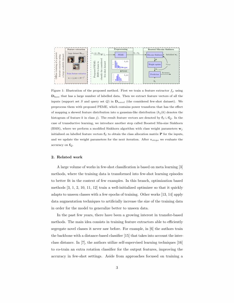
Figure 1: Illustration of the proposed method. First we train a feature extractor fϕ using

Dbase that has a large number of labelled data. Then we extract feature vectors of all the

inputs (support set S and query set Q) in Dnovel (the considered few-shot dataset). We

preprocess them with proposed PEME, which contains power transform that has the effect

of mapping a skewed feature distribution into a gaussian-like distribution (hj(k) denotes the

histogram of feature k in class j). The result feature vectors are denoted by fS ∪ fQ. In the

case of transductive learning, we introduce another step called Boosted Min-size Sinkhorn

(BMS), where we perform a modified Sinkhorn algorithm with class weight parameters wj

initialized on labelled feature vectors fS to obtain the class allocation matrix P for the inputs,

and we update the weight parameters for the next iteration. After nsteps we evaluate the

accuracy on fQ.

2. Related work

A large volume of works in few-shot classification is based on meta learning [3]

methods, where the training data is transformed into few-shot learning episodes

to better fit in the context of few examples. In this branch, optimization based

methods [3, 1, 2, 10, 11, 12] train a well-initialized optimizer so that it quickly

adapts to unseen classes with a few epochs of training. Other works [13, 14] apply

data augmentation techniques to artificially increase the size of the training data

in order for the model to generalize better to unseen data.

In the past few years, there have been a growing interest in transfer-based

methods. The main idea consists in training feature extractors able to efficiently

segregate novel classes it never saw before. For example, in [6] the authors train

the backbone with a distance-based classifier [15] that takes into account the inter-

class distance. In [7], the authors utilize self-supervised learning techniques [16]

to co-train an extra rotation classifier for the output features, improving the

accuracy in few-shot settings. Aside from approaches focused on training a

3

more robust model, other approaches are built on top of a pre-trained feature

extractor (backbone). For instance, in [17] the authors implement a nearest class

mean classifier to associate an input with a class whose centroid is the closest

in terms of the `2 distance. In [18] an iterative approach is used to adjust the

class prototypes. In [8] the authors build a graph neural network to gather the

feature information from similar samples. Generally, transfer-based techniques

often reach the best performance on standardized benchmarks.

Although many works involve feature extraction, few have explored the

features in terms of their distribution [19, 20, 7]. Often, assumptions are made

that the features in a class align to a certain distribution, even though these

assumptions are seldom experimentally discussed. In our work, we analyze the

impact of the features distributions and how they can be transformed for better

processing and accuracy. We also introduce a new algorithm to improve the

quality of the association between input features and corresponding classes in

typical few-shot settings.

Contributions. Let us highlight the main contributions of this work. (1)

We propose to preprocess the raw extracted features in order to make them more

aligned with Gaussian assumptions. Namely we introduce transforms of the

features so that they become less skewed. (2) We use a Wasserstein-based method

to better align the distribution of features with that of the considered classes.

(3) We show that the proposed method can bring large increase in accuracy with

a variety of feature extractors and datasets, leading to state-of-the-art results

in the considered benchmarks. This work is an extended version of [9], with

the main difference that here we consider the broader case where we do not

know the proportion of samples belonging to each considered class in the case

of transductive few-shot, leading to a new algorithm called Boosted Min-size

Sinkhorn. We also propose more efficient preprocessing steps, leading to overall

better performance in both inductive and transductive settings. Finally, we

introduce the use of Logistic Regression in our methodology instead of a simple

Nearest Class Mean classifier.

4

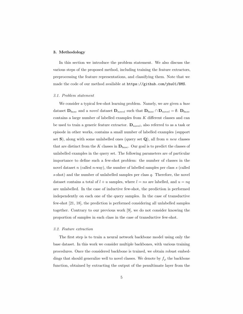
3. Methodology

In this section we introduce the problem statement. We also discuss the

various steps of the proposed method, including training the feature extractors,

preprocessing the feature representations, and classifying them. Note that we

made the code of our method available at https://github.com/yhu01/BMS.

3.1. Problem statement

We consider a typical few-shot learning problem. Namely, we are given a base

dataset Dbase and a novel dataset Dnovel such that Dbase ∩Dnovel = ∅. Dbase

contains a large number of labelled examples from K different classes and can

be used to train a generic feature extractor. Dnovel, also referred to as a task or

episode in other works, contains a small number of labelled examples (support

set S), along with some unlabelled ones (query set Q), all from n new classes

that are distinct from the K classes in Dbase. Our goal is to predict the classes of

unlabelled examples in the query set. The following parameters are of particular

importance to define such a few-shot problem: the number of classes in the

novel dataset n (called n-way), the number of labelled samples per class s (called

s-shot) and the number of unlabelled samples per class q. Therefore, the novel

dataset contains a total of l + u samples, where l = ns are labelled, and u = nq

are unlabelled. In the case of inductive few-shot, the prediction is performed

independently on each one of the query samples. In the case of transductive

few-shot [21, 18], the prediction is performed considering all unlabelled samples

together. Contrary to our previous work [9], we do not consider knowing the

proportion of samples in each class in the case of transductive few-shot.

3.2. Feature extraction

The first step is to train a neural network backbone model using only the

base dataset. In this work we consider multiple backbones, with various training

procedures. Once the considered backbone is trained, we obtain robust embed-

dings that should generalize well to novel classes. We denote by fϕ the backbone

function, obtained by extracting the output of the penultimate layer from the

5

considered architecture, with ϕ being the trained architecture parameters. Thus

considering an input vector x, fϕ(x) is a feature vector with d dimensions that

can be thought of as a simpler-to-manipulate representation of x. Note that

importantly, in all backbone architectures used in the experiments of this work,

the penultimate layers are obtained by applying a ReLU function, so that all

feature components coming out of fϕ are nonnegative.

3.3. Feature preprocessing

As mentioned in Section 2, many works hypothesize, explicitly or not, that

the features from the same class are aligned with a specific distribution (often

Gaussian-like). But this aspect is rarely experimentally verified. In fact, it is very

likely that features obtained using the backbone architecture are not Gaussian.

Indeed, usually the features are obtained after applying a ReLU function [22],

and exhibit a positive and yet skewed distribution mostly concentrated around 0

(more details can be found in the next section).

Multiple works in the domain [17, 18] discuss the different statistical methods

(e.g. batch normalization) to better fit the features into a model. Although

these methods may have provable assets for some distributions, they could

worsen the process if applied to an unexpected input distribution. This is

why we propose to preprocess the obtained raw feature vectors so that they

better align with typical distribution assumptions in the field. Denote fϕ(x) =

[f1ϕ(x), ..., fhϕ(x), ..., fdϕ(x)] ∈ (R+)d,x ∈ Dnovel as the obtained features on

Dnovel, and fhϕ(x), 1 ≤ h ≤ d denotes its value in the hth position. The

preprocessing methods applied in our proposed algorithms are as follows:

Euclidean normalization. Also known as L2-normalization that is widely

used in many related works [17, 20, 8], this step scales the features to the

same area so that large variance feature vectors do not predominate the others.

Euclidean normalization can be given by:

fϕ(x)← fϕ(x)

‖fϕ(x)‖2(1)

Power transform. Power transform method [23, 9] simply consists of taking

6

the power of each feature vector coordinate. The formula is given by:

fhϕ(x)← (fhϕ(x) + ε)β , β 6= 0 (2)

where ε = 1e− 6 is used to make sure that fϕ(x) + ε is strictly positive in every

position, and β is a hyper-parameter. The rationale of the preprocessing above

is that power transform, often used in combination with euclidean normalization,

has the functionality of reducing the skew of a distribution and mapping it to

a close-to-gaussian distribution, adjusted by β. After experiments, we found

that β = 0.5 gives the most consistent results for our considered experiments,

which corresponds to a square-root function that has a wide range of usage on

features [24]. We will analyse this ability and the effect of power transform in

more details in Section 4. Note that power transform can only be applied if

considered feature vectors contain nonnegative entries, which will always be the

case in the remaining of this work.

Mean subtraction. With mean subtraction, each sample is translated

using m ∈ (R+)d, the projection center. This is often used in combination with

euclidean normalization in order to reduce the task bias and better align the

feature distributions [18]. The formula is given by:

fϕ(x)← fϕ(x)−m (3)

The projection center is often computed as the mean values of feature vectors

related to the problem [17, 18]. In this paper we compute it either as the mean

feature vector of the base dataset (denoted as Mb) or the mean vector of the

novel dataset (denoted as Mn), depending on the few-shot settings. Of course,

in both of these cases, the rationale is to consider a proxy to what would be the

exact mean value of feature vectors on the considered task.

In our proposed method we deploy these preprocessing steps in the following

order: Power transform (P) on the raw features, followed by an Euclidean

normalization (E). Then we perform Mean subtraction (M) followed by another

Euclidean normalization at the end. For simplicity we denote PEME as our

proposed preprocessing order, in which M can be either Mb or Mn as mentioned

7

above. In our experiments, we found that using Mb in the case of inductive few-

shot learning and Mn in the case of transductive few-shot learning consistently led

to the most competitive results. More details on why we used this methodology

are available in the experiment section.

When facing an inductive problem, a simple classifier such as a Nearest-Class-

Mean classifier (NCM) can be used directly after this preprocessing step. The

resulting methodology is denoted PEMbE-NCM. But in the case of transductive

settings, we also introduce an iterative procedure, denoted BMS for Boosted

Min-size Sinkhorn, meant to leverage the joint distribution of unlabelled samples.

The resulting methodology is denoted PEMnE-BMS. The details of the BMS

procedure are presented thereafter.

3.4. Boosted Min-size Sinkhorn

In the case of transductive few-shot, we introduce a method that consists in

iteratively refining estimates for the probability each unlabelled sample belong

to any of the considered classes. This method is largely based on the one we

introduced in [9], except it does not require priors about samples distribution

in each of the considered class. Denote i ∈ [1, ..., l + u] as the sample index in

Dnovel and j ∈ [1, ..., n] as the class index, the goal is to maximize the following

log post-posterior function:

L(θ) =∑i

logP (l(xi) = j|xi; θ)

=∑i

logP (xi, l(xi) = j; θ)

P (xi; θ)

∝∑i

logP (xi|l(xi) = j; θ)

P (xi; θ),

(4)

here l(xi) denotes the class label for sample xi ∈ Q ∪ S, P (xi; θ) denotes

the marginal probability, and θ represents the model parameters to estimate.

Assuming a gaussian distribution on the input features for each class, here we

define θ = wj ,∀j where wj ∈ Rd stand for the weight parameters for class j.

We observe that Eq. 4 can be related to the cost function utilized in Optimal

Transport [25], which is often considered to solve classification problems, with

8

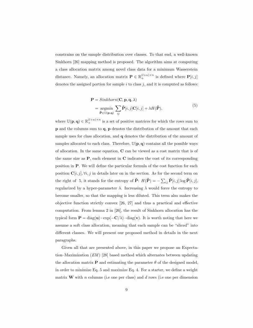
constrains on the sample distribution over classes. To that end, a well-known

Sinkhorn [26] mapping method is proposed. The algorithm aims at computing

a class allocation matrix among novel class data for a minimum Wasserstein

distance. Namely, an allocation matrix P ∈ R(l+u)×n+ is defined where P[i, j]

denotes the assigned portion for sample i to class j, and it is computed as follows:

P = Sinkhorn(C,p,q, λ)

= argminP∈U(p,q)

∑ij

P[i, j]C[i, j] + λH(P),(5)

where U(p,q) ∈ R(l+u)×n+ is a set of positive matrices for which the rows sum to

p and the columns sum to q, p denotes the distribution of the amount that each

sample uses for class allocation, and q denotes the distribution of the amount of

samples allocated to each class. Therefore, U(p,q) contains all the possible ways

of allocation. In the same equation, C can be viewed as a cost matrix that is of

the same size as P, each element in C indicates the cost of its corresponding

position in P. We will define the particular formula of the cost function for each

position C[i, j],∀i, j in details later on in the section. As for the second term on

the right of 5, it stands for the entropy of P: H(P) = −∑ij P[i, j] log P[i, j],

regularized by a hyper-parameter λ. Increasing λ would force the entropy to

become smaller, so that the mapping is less diluted. This term also makes the

objective function strictly convex [26, 27] and thus a practical and effective

computation. From lemma 2 in [26], the result of Sinkhorn allocation has the

typical form P = diag(u) · exp(−C/λ) · diag(v). It is worth noting that here we

assume a soft class allocation, meaning that each sample can be “sliced” into

different classes. We will present our proposed method in details in the next

paragraphs.

Given all that are presented above, in this paper we propose an Expecta-

tion–Maximization (EM ) [28] based method which alternates between updating

the allocation matrix P and estimating the parameter θ of the designed model,

in order to minimize Eq. 5 and maximize Eq. 4. For a starter, we define a weight

matrix W with n columns (i.e one per class) and d rows (i.e one per dimension

9

of feature vectors), for column j in W we denote it as the weight parameters

wj ∈ Rd for class j in correspondence with Eq. 4. And it is initialized as follows:

wj = W[:, j] = cj/‖cj‖2, (6)

where

cj =1

s

∑x∈S,`(x)=j

fϕ(x). (7)

We can see that W contains the average of feature vectors in the support set for

each class, followed by a L2-normalization on each column so that ‖wj‖2 = 1,∀j.

Then, we iterate multiple steps that we describe thereafter.

a. Computing costs

As previously stated, the proposed algorithm is an EM -like one that iterately

updates model parameters for optimal estimates. Therefore, this step along with

Min-size Sinkhorn presented in the next step, is considered as the E -step of our

proposed method. The goal is to find membership probabilities for the input

samples, namely, we compute P that minimizes Eq. 5.

Here we assume gaussian distributions, features in each class have the same

variance and are independent from one another (covariance matrix Σ = Iσ2).

We observe that, ignoring the marginal probability, Eq. 4 can be boiled down to

negative L2 distances between extracted samples fϕ(xi),∀i and wj ,∀j, which

is initialized in Eq. 6 in our proposed method. Therefore, based on the fact

that wj and fϕ(xi) are both normalized to be unit length vectors (fϕ(xi) being

preprocessed using PEME introduced in the previous section), here we define

the cost between sample i and class j to be the following equation:

C[i, j] ∝ (fϕ(xi)−wj)2

= 1−wTj fϕ(xi),

(8)

which corresponds to the cosine distance.

b. Min-size Sinkhorn

In [9], we proposed a Wasserstein distance based method in which the

Sinkhorn algorithm is applied at each iteration so that the class prototypes are

10

Algorithm 1 Min-size Sinkhorn

Inputs: C,p = 1l+u,q = k1n, λ

Initializations: P = Softmax(−λC)

for iter = 1 to 50 do

P[i, :]← p[i] · P[i,:]∑j P[i,j] ,∀i

P[:, j]← q[j] · P[:,j]∑i P[i,j] if

∑i P[i, j] < q[j],∀j

end for

return P

updated iteratively in order to find their best estimates. Although the method

showed promising results, it is established on the condition that the distribution

of the query set is known, e.g. a uniform distribution among classes on the query

set. This is not ideal given the fact that any priors about Q should be supposedly

kept unknown when applying a method. The methodology introduced in this

paper can be seen as a generalization of that introduced in [9] that does not

require priors about Q.

In the classical settings, Sinkhorn algorithm aims at finding the optimal

matrix P, given the cost matrix C and regulation parameter λ presented in

Eq. 4). Typically it initiates P from a softmax operation over the rows in C,

then it iterates between normalizing columns and rows of P, until the resulting

matrix becomes close-to doubly stochastic according to p and q. However, in

our case we do not know the distribution of samples over classes. To address

this, we firstly introduce the parameter k, initialized so that k ← s, meant to

track an estimate of the cardinal of the class containing the least number of

samples in the considered task. Then we propose the following modification to

be applied to the matrix P once initialized: we normalize each row as in the

classical case, but only normalize the columns of P for which the sum is less

than the previously computed min-size k [18]. This ensures at least k elements

allocated for each class, but not exactly k samples as in the balanced case.

The principle of this modified Sinkhorn solution is presented in Algorithm 1.

c. Updating weights

11

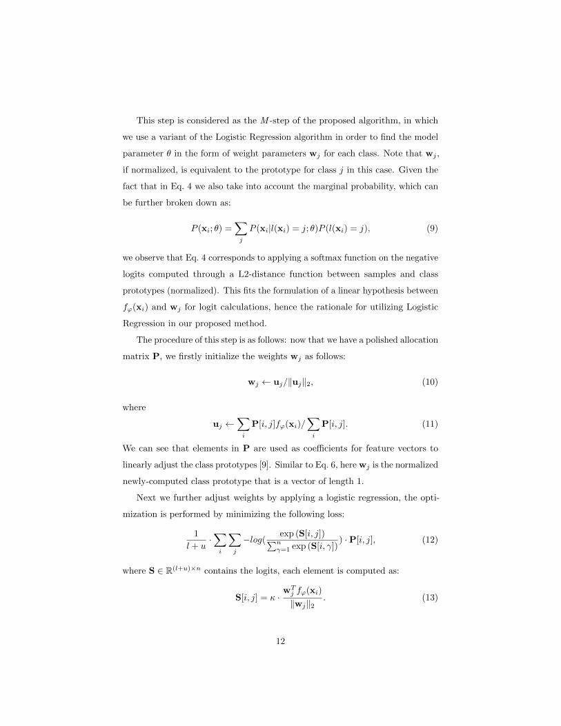
This step is considered as the M -step of the proposed algorithm, in which

we use a variant of the Logistic Regression algorithm in order to find the model

parameter θ in the form of weight parameters wj for each class. Note that wj ,

if normalized, is equivalent to the prototype for class j in this case. Given the

fact that in Eq. 4 we also take into account the marginal probability, which can

be further broken down as:

P (xi; θ) =∑j

P (xi|l(xi) = j; θ)P (l(xi) = j), (9)

we observe that Eq. 4 corresponds to applying a softmax function on the negative

logits computed through a L2-distance function between samples and class

prototypes (normalized). This fits the formulation of a linear hypothesis between

fϕ(xi) and wj for logit calculations, hence the rationale for utilizing Logistic

Regression in our proposed method.

The procedure of this step is as follows: now that we have a polished allocation

matrix P, we firstly initialize the weights wj as follows:

wj ← uj/‖uj‖2, (10)

where

uj ←∑i

P[i, j]fϕ(xi)/∑i

P[i, j]. (11)

We can see that elements in P are used as coefficients for feature vectors to

linearly adjust the class prototypes [9]. Similar to Eq. 6, here wj is the normalized

newly-computed class prototype that is a vector of length 1.

Next we further adjust weights by applying a logistic regression, the opti-

mization is performed by minimizing the following loss:

1

l + u·∑i

∑j

−log(exp (S[i, j])∑nγ=1 exp (S[i, γ])

) ·P[i, j], (12)

where S ∈ R(l+u)×n contains the logits, each element is computed as:

S[i, j] = κ ·wTj fϕ(xi)

‖wj‖2. (13)

12

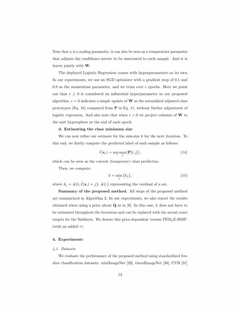
Note that κ is a scaling parameter, it can also be seen as a temperature parameter

that adjusts the confidence metric to be associated to each sample. And it is

learnt jointly with W.

The deployed Logistic Regression comes with hyperparameters on its own.

In our experiments, we use an SGD optimizer with a gradient step of 0.1 and

0.8 as the momentum parameter, and we train over e epochs. Here we point

out that e ≥ 0 is considered an influential hyperparameter in our proposed

algorithm, e = 0 indicates a simple update of W as the normalized adjusted class

prototypes (Eq. 10) computed from P in Eq. 11, without further adjustment of

logistic regression. And also note that when e > 0 we project columns of W to

the unit hypersphere at the end of each epoch.

d. Estimating the class minimum size

We can now refine our estimate for the min-size k for the next iteration. To

this end, we firstly compute the predicted label of each sample as follows:

ˆ(xi) = arg maxj

(P[i, j]), (14)

which can be seen as the current (temporary) class prediction.

Then, we compute:

k = minj{kj}, (15)

where kj = #{i, ˆ(xi) = j}, #{·} representing the cardinal of a set.

Summary of the proposed method. All steps of the proposed method

are summarized in Algorithm 2. In our experiments, we also report the results

obtained when using a prior about Q as in [9]. In this case, k does not have to

be estimated throughout the iterations and can be replaced with the actual exact

targets for the Sinkhorn. We denote this prior-dependent version PEMnE-BMS∗

(with an added ∗).

4. Experiments

4.1. Datasets

We evaluate the performance of the proposed method using standardized few-

shot classification datasets: miniImageNet [29], tieredImageNet [30], CUB [31]

13

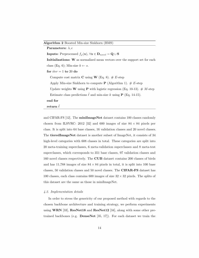
Algorithm 2 Boosted Min-size Sinkhorn (BMS)

Parameters: λ, e

Inputs: Preprocessed fϕ(x), ∀x ∈ Dnovel = Q ∪ S

Initializations: W as normalized mean vectors over the support set for each

class (Eq. 6); Min-size k ← s.

for iter = 1 to 20 do

Compute cost matrix C using W (Eq. 8). # E-step

Apply Min-size Sinkhorn to compute P (Algorithm 1). # E-step

Update weights W using P with logistic regression (Eq. 10-13). # M -step

Estimate class predictions ˆ and min-size k using P (Eq. 14-15).

end for

return ˆ

and CIFAR-FS [12]. The miniImageNet dataset contains 100 classes randomly

chosen from ILSVRC- 2012 [32] and 600 images of size 84 × 84 pixels per

class. It is split into 64 base classes, 16 validation classes and 20 novel classes.

The tieredImageNet dataset is another subset of ImageNet, it consists of 34

high-level categories with 608 classes in total. These categories are split into

20 meta-training superclasses, 6 meta-validation superclasses and 8 meta-test

superclasses, which corresponds to 351 base classes, 97 validation classes and

160 novel classes respectively. The CUB dataset contains 200 classes of birds

and has 11,788 images of size 84 × 84 pixels in total, it is split into 100 base

classes, 50 validation classes and 50 novel classes. The CIFAR-FS dataset has

100 classes, each class contains 600 images of size 32× 32 pixels. The splits of

this dataset are the same as those in miniImageNet.

4.2. Implementation details

In order to stress the genericity of our proposed method with regards to the

chosen backbone architecture and training strategy, we perform experiments

using WRN [33], ResNet18 and ResNet12 [34], along with some other pre-

trained backbones (e.g. DenseNet [35, 17]). For each dataset we train the

14

feature extractor with base classes and test the performance using novel classes.

Therefore, for each test run, n classes are drawn uniformly at random among

novel classes. Among these n classes, s labelled examples and q unlabelled ex-

amples per class are uniformly drawn at random to form Dnovel. The WRN and

ResNet are trained following [7]. In the inductive setting, we use our proposed

preprocessing steps PEMbE followed by a basic Nearest Class Mean (NCM)

classifier. In the transductive setting, the preprocessing steps are denoted as

PEMnE in that we use the mean vector of novel dataset for mean subtraction,

followed by BMS or BMS∗ depending on whether we have prior knowledge on

the distribution of query set Q among classes. Note that we perform a QR

decomposition on preprocessed features in order to speed up the computation for

the classifier that follows. All our experiments are performed using n = 5, q = 15,

s = 1 or 5. We run 10,000 random draws to obtain mean accuracy score and

indicate confidence scores (95%) when relevant. For our proposed PEMnE-BMS,

we train e = 0 epoch in the case of 1-shot and e = 40 epochs in the case of

5-shot. As for PEMnE-BMS∗ we set e = 20 for 1-shot and e = 40 for 5-shot.

As for the regularization parameter λ in Eq. 5, it is fixed to 8.5 for all settings.

Impact of these hyperparameters is detailed in the next sections.

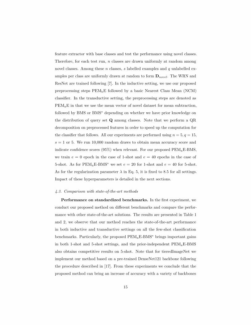
4.3. Comparison with state-of-the-art methods

Performance on standardized benchmarks. In the first experiment, we

conduct our proposed method on different benchmarks and compare the perfor-

mance with other state-of-the-art solutions. The results are presented in Table 1

and 2, we observe that our method reaches the state-of-the-art performance

in both inductive and transductive settings on all the few-shot classification

benchmarks. Particularly, the proposed PEMnE-BMS∗ brings important gains

in both 1-shot and 5-shot settings, and the prior-independent PEMnE-BMS

also obtains competitive results on 5-shot. Note that for tieredImageNet we

implement our method based on a pre-trained DenseNet121 backbone following

the procedure described in [17]. From these experiments we conclude that the

proposed method can bring an increase of accuracy with a variety of backbones

15

and datasets, leading to state-of-the-art performance. In terms of execution

time, we measured an average of 0.004s per run.

Performance on cross-domain settings. In this experiment we test our

method in a cross-domain setting, where the backbone is trained with the base

classes in miniImageNet but tested with the novel classes in CUB dataset. As

shown in Table 3, the proposed method gives the best accuracy both in the case

of 1-shot and 5-shot, for both inductive and transductive settings.

4.4. Ablation studies

Generalization to backbone architectures. To further stress the inter-

est of the ingredients on the proposed method reaching top performance, in

Table 4 we investigate the impact of our proposed method on different backbone

architectures and benchmarks in the transductive setting. For comparison pur-

pose we also replace our proposed BMS algorithm with a standard K-Means

algorithm where class prototypes are initialized with the available labelled sam-

ples for each class. We can observe that: 1) the proposed method consistently

achieves the best results for any fixed backbone architecture, 2) the feature

extractor trained on WRN outperforms the others with our proposed method on

different benchmarks, 3) there are significant drops in accuracy with K-Means,

which stresses the interest of BMS, and 4) the prior on Q (BMS vs BMS∗) has

major interest for 1-shot, boosting the performance by an approximation of 1%

on all tested feature extractors.

Preprocessing impact. In Table 5 we compare our proposed PEME with

other preprocessing techniques such as Batch Normalization and the ones being

used in [17]. The experiment is conducted on miniImageNet (backbone: WRN).

For all that are put into comparison, we run either a NCM classifier or BMS after

preprocessing, depending on the settings. The obtained results clearly show the

interest of PEME compared with existing alternatives, we also observe that the

power transform helps increase the accuracy on both inductive and transductive

settings. We will further study its impact in details.

Effect of power transform. We firstly conduct a Gaussian hypothesis test

16

Table 1: 1-shot and 5-shot accuracy of state-of-the-art methods in the literature on miniIma-

geNet and tieredImageNet, compared with the proposed solution.

miniImageNet

Setting Method Backbone 1-shot 5-shot

Inductive

Matching Networks [29] WRN 64.03± 0.20% 76.32± 0.16%

SimpleShot [17] DenseNet121 64.29± 0.20% 81.50± 0.14%

S2M2 R [7] WRN 64.93± 0.18% 83.18± 0.11%

PT+NCM [9] WRN 65.35± 0.20% 83.87± 0.13%

DeepEMD[36] ResNet12 65.91± 0.82% 82.41± 0.56%

FEAT[37] ResNet12 66.78± 0.20% 82.05± 0.14%

PEMbE-NCM (ours) WRN 68.43± 0.20% 84.67± 0.13%

Transductive

BD-CSPN [38] WRN 70.31± 0.93% 81.89± 0.60%

LaplacianShot [39] DenseNet121 75.57± 0.19% 87.72± 0.13%

Transfer+SGC [8] WRN 76.47± 0.23% 85.23± 0.13%

TAFSSL [18] DenseNet121 77.06± 0.26% 84.99± 0.14%

TIM-GD [40] WRN 77.80% 87.40%

MCT [41] ResNet12 78.55± 0.86% 86.03± 0.42%

EPNet [42] WRN 79.22± 0.92% 88.05± 0.51%

PT+MAP [9] WRN 82.92± 0.26% 88.82± 0.13%

PEMnE-BMS (ours) WRN 82.07± 0.25% 89.51± 0.13%

PEMnE-BMS∗ (ours) WRN 83.35± 0.25% 89.53± 0.13%

tieredImageNet

Setting Method Backbone 1-shot 5-shot

Inductive

ProtoNet [43] ConvNet4 53.31± 0.89% 72.69± 0.74%

LEO [44] WRN 66.33± 0.05% 81.44± 0.09%

SimpleShot [17] DenseNet121 71.32± 0.22% 86.66± 0.15%

PT+NCM [9] DenseNet121 69.96± 0.22% 86.45± 0.15%

FEAT[37] ResNet12 70.80± 0.23% 84.79± 0.16%

DeepEMD[36] ResNet12 71.16± 0.87% 86.03± 0.58%

RENet[45] ResNet12 71.61± 0.51% 85.28± 0.35%

PEMbE-NCM (ours) DenseNet121 71.86± 0.21% 87.09± 0.15%

Transductive

BD-CSPN [38] WRN 78.74± 0.95% 86.92± 0.63%

LaplacianShot [39] DenseNet121 80.30± 0.22% 87.93± 0.15%

MCT [41] ResNet12 82.32± 0.81% 87.36± 0.50%

TIM-GD [40] WRN 82.10% 89.80%

TAFSSL [18] DenseNet121 84.29± 0.25% 89.31± 0.15%

PT+MAP [9] DenseNet121 85.75± 0.26% 90.43± 0.14%

PEMnE-BMS (ours) DenseNet121 85.08± 0.25% 91.08± 0.14%

PEMnE-BMS∗ (ours) DenseNet121 86.07± 0.25% 91.09± 0.14%

17

Table 2: 1-shot and 5-shot accuracy of state-of-the-art methods on CUB and CIFAR-FS.

CUB

Setting Method Backbone 1-shot 5-shot

Inductive

Baseline++ [6] ResNet10 69.55± 0.89% 85.17± 0.50%

MAML [1] ResNet10 70.32± 0.99% 80.93± 0.71%

ProtoNet [43] ResNet18 72.99± 0.88% 86.64± 0.51%

Matching Networks [29] ResNet18 73.49± 0.89% 84.45± 0.58%

FEAT[37] ResNet12 73.27± 0.22% 85.77± 0.14%

DeepEMD[36] ResNet12 75.65± 0.83% 88.69± 0.50%

RENet[45] ResNet12 79.49± 0.44% 91.11± 0.24%

S2M2 R [7] WRN 80.68± 0.81% 90.85± 0.44%

PT+NCM [9] WRN 80.57± 0.20% 91.15± 0.10%

PEMbE-NCM (ours) WRN 80.82± 0.19% 91.46± 0.10%

Transductive

LaplacianShot [39] ResNet18 80.96% 88.68%

TIM-GD [40] ResNet18 82.20% 90.80%

BD-CSPN [38] WRN 87.45% 91.74%

Transfer+SGC [8] WRN 88.35± 0.19% 92.14± 0.10%

PT+MAP [9] WRN 91.55± 0.19% 93.99± 0.10%

LST+MAP [46] WRN 91.68± 0.19% 94.09± 0.10%

PEMnE-BMS (ours) WRN 91.01± 0.19% 94.60± 0.09%

PEMnE-BMS∗ (ours) WRN 91.91± 0.18% 94.62± 0.09%

CIFAR-FS

Setting Method Backbone 1-shot 5-shot

Inductive

ProtoNet [43] ConvNet64 55.50± 0.70% 72.00± 0.60%

MAML [1] ConvNet32 58.90± 1.90% 71.50± 1.00%

RENet[45] ResNet12 74.51± 0.46% 86.60± 0.32%

BD-CSPN [38] WRN 72.13± 1.01% 82.28± 0.69%

S2M2 R [7] WRN 74.81± 0.19% 87.47± 0.13%

PT+NCM [9] WRN 74.64± 0.21% 87.64± 0.15%

PEMbE-NCM (ours) WRN 74.84± 0.21% 87.73± 0.15%

Transductive

DSN-MR [47] ResNet12 78.00± 0.90% 87.30± 0.60%

Transfer+SGC [8] WRN 83.90± 0.22% 88.76± 0.15%

MCT [41] ResNet12 87.28± 0.70% 90.50± 0.43%

PT+MAP [9] WRN 87.69± 0.23% 90.68± 0.15%

LST+MAP [46] WRN 87.79± 0.23% 90.73± 0.15%

PEMnE-BMS (ours) WRN 86.93± 0.23% 91.18± 0.15%

PEMnE-BMS∗ (ours) WRN 87.83± 0.22% 91.20± 0.15%

on each of the 640 coordinates of raw extracted features (backbone: WRN) for

each of the 20 novel classes (dataset: miniImageNet). Following D’Agostino and

18

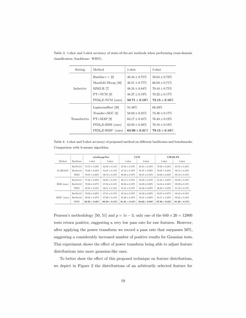
Table 3: 1-shot and 5-shot accuracy of state-of-the-art methods when performing cross-domain

classification (backbone: WRN).

Setting Method 1-shot 5-shot

Inductive

Baseline++ [6] 40.44± 0.75% 56.64± 0.72%

Manifold Mixup [48] 46.21± 0.77% 66.03± 0.71%

S2M2 R [7] 48.24± 0.84% 70.44± 0.75%

PT+NCM [9] 48.37± 0.19% 70.22± 0.17%

PEMbE-NCM (ours) 50.71± 0.19% 73.15± 0.16%

Transductive

LaplacianShot [39] 55.46% 66.33%

Transfer+SGC [8] 58.63± 0.25% 73.46± 0.17%

PT+MAP [9] 63.17± 0.31% 76.43± 0.19%

PEMnE-BMS (ours) 62.93± 0.28% 79.10± 0.18%

PEMnE-BMS∗ (ours) 63.90± 0.31% 79.15± 0.18%

Table 4: 1-shot and 5-shot accuracy of proposed method on different backbones and benchmarks.

Comparison with k-means algorithm.

miniImageNet CUB CIFAR-FS

Method Backbone 1-shot 5-shot 1-shot 5-shot 1-shot 5-shot

K-MEANS

ResNet12 72.73± 0.23% 84.05± 0.14% 87.35± 0.19% 92.31± 0.10% 78.39± 0.24% 85.73± 0.16%

ResNet18 73.08± 0.22% 84.67± 0.14% 87.16± 0.19% 91.97± 0.09% 79.95± 0.23% 86.74± 0.16%

WRN 76.67± 0.22% 86.73± 0.13% 88.28± 0.19% 92.37± 0.10% 83.69± 0.22% 89.19± 0.15%

BMS (ours)

ResNet12 77.62± 0.28% 86.95± 0.15% 90.14± 0.19% 94.30± 0.10% 81.65± 0.25% 88.38± 0.16%

ResNet18 79.30± 0.27% 87.94± 0.14% 90.50± 0.19% 94.29± 0.09% 84.16± 0.24% 89.39± 0.15%

WRN 82.07± 0.25% 89.51± 0.13% 91.01± 0.18% 94.60± 0.09% 86.93± 0.23% 91.18± 0.15%

BMS∗ (ours)

ResNet12 79.03± 0.28% 87.01± 0.15% 91.34± 0.19% 94.32± 0.09% 82.87± 0.27% 88.43± 0.16%

ResNet18 80.56± 0.27% 87.98± 0.14% 91.39± 0.19% 94.31± 0.09% 85.17± 0.25% 89.42± 0.16%

WRN 83.35± 0.25% 89.53± 0.13% 91.91± 0.18% 94.62± 0.09% 87.83± 0.22% 91.20± 0.15%

Pearson’s methodology [50, 51] and p = 1e− 3, only one of the 640× 20 = 12800

tests return positive, suggesting a very low pass rate for raw features. However,

after applying the power transform we record a pass rate that surpasses 50%,

suggesting a considerably increased number of positive results for Gaussian tests.

This experiment shows the effect of power transform being able to adjust feature

distributions into more gaussian-like ones.

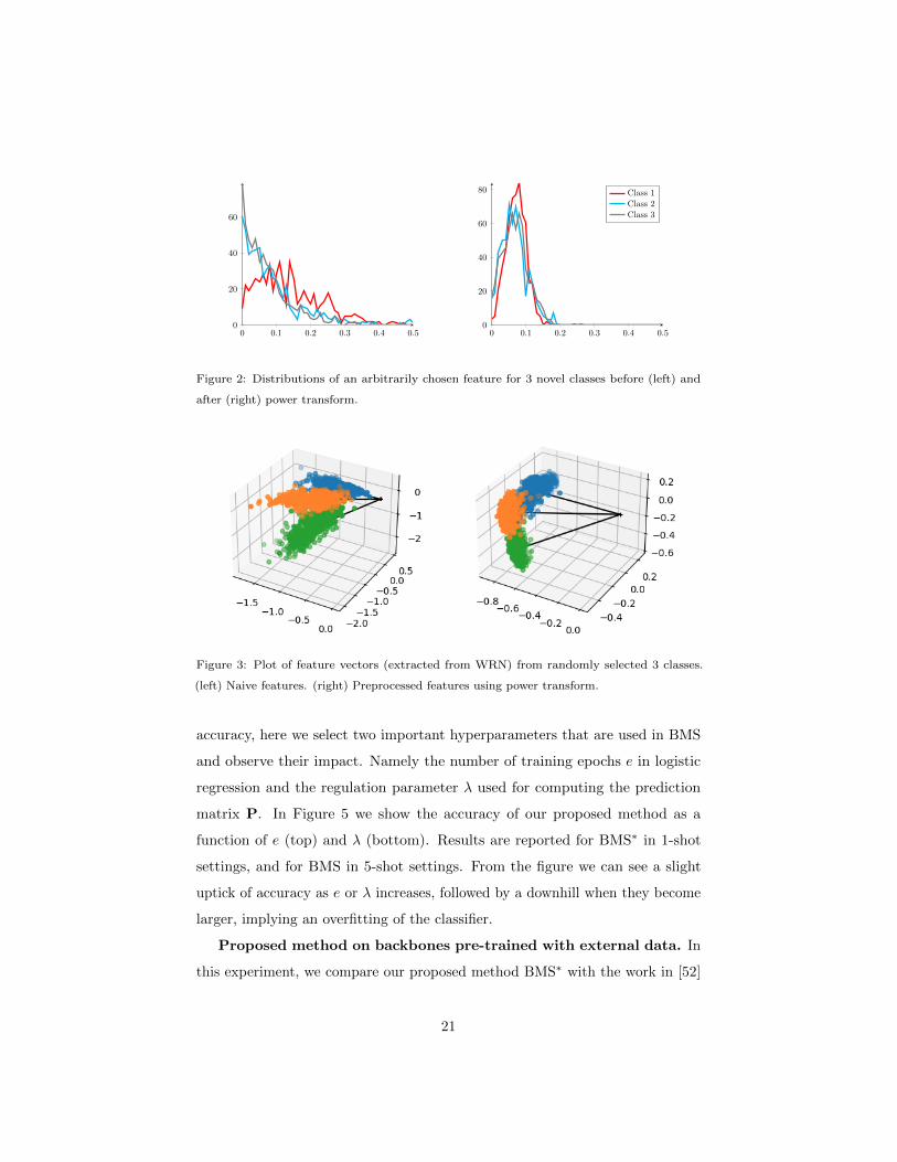
To better show the effect of this proposed technique on feature distributions,

we depict in Figure 2 the distributions of an arbitrarily selected feature for

19

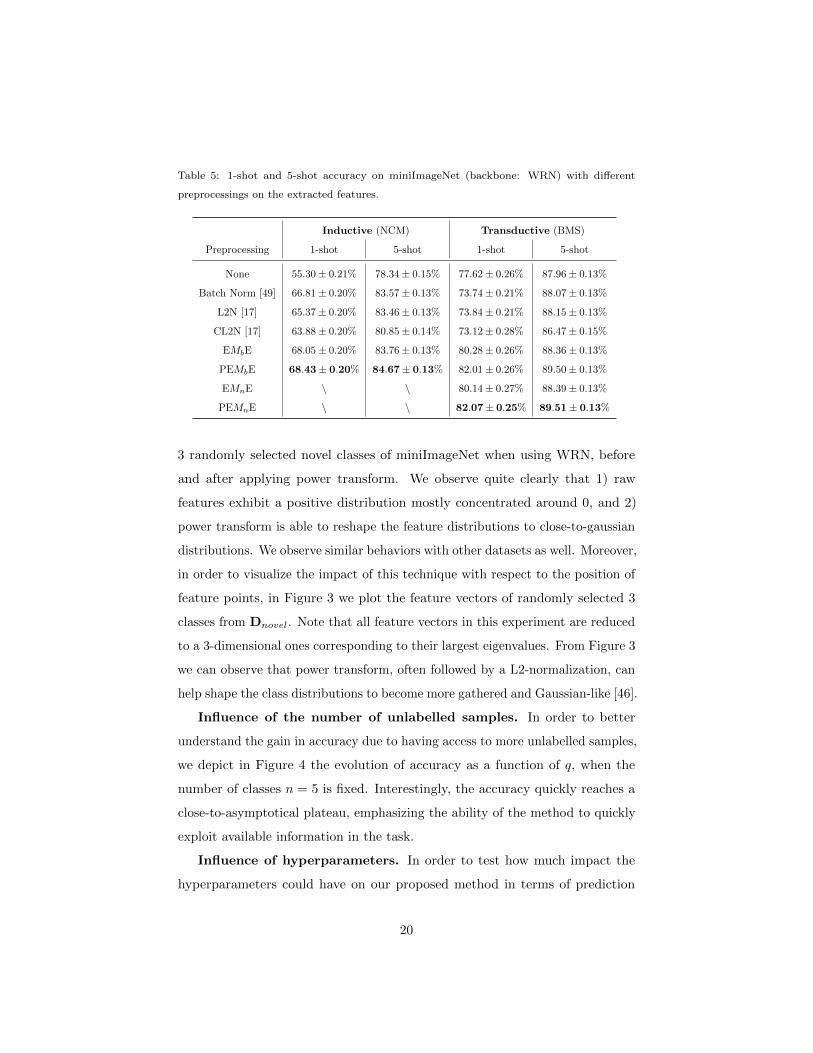
Table 5: 1-shot and 5-shot accuracy on miniImageNet (backbone: WRN) with different

preprocessings on the extracted features.

Inductive (NCM) Transductive (BMS)

Preprocessing 1-shot 5-shot 1-shot 5-shot

None 55.30± 0.21% 78.34± 0.15% 77.62± 0.26% 87.96± 0.13%

Batch Norm [49] 66.81± 0.20% 83.57± 0.13% 73.74± 0.21% 88.07± 0.13%

L2N [17] 65.37± 0.20% 83.46± 0.13% 73.84± 0.21% 88.15± 0.13%

CL2N [17] 63.88± 0.20% 80.85± 0.14% 73.12± 0.28% 86.47± 0.15%

EMbE 68.05± 0.20% 83.76± 0.13% 80.28± 0.26% 88.36± 0.13%

PEMbE 68.43± 0.20% 84.67± 0.13% 82.01± 0.26% 89.50± 0.13%

EMnE \ \ 80.14± 0.27% 88.39± 0.13%

PEMnE \ \ 82.07± 0.25% 89.51± 0.13%

3 randomly selected novel classes of miniImageNet when using WRN, before

and after applying power transform. We observe quite clearly that 1) raw

features exhibit a positive distribution mostly concentrated around 0, and 2)

power transform is able to reshape the feature distributions to close-to-gaussian

distributions. We observe similar behaviors with other datasets as well. Moreover,

in order to visualize the impact of this technique with respect to the position of

feature points, in Figure 3 we plot the feature vectors of randomly selected 3

classes from Dnovel. Note that all feature vectors in this experiment are reduced

to a 3-dimensional ones corresponding to their largest eigenvalues. From Figure 3

we can observe that power transform, often followed by a L2-normalization, can

help shape the class distributions to become more gathered and Gaussian-like [46].

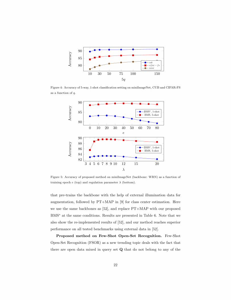
Influence of the number of unlabelled samples. In order to better

understand the gain in accuracy due to having access to more unlabelled samples,

we depict in Figure 4 the evolution of accuracy as a function of q, when the

number of classes n = 5 is fixed. Interestingly, the accuracy quickly reaches a

close-to-asymptotical plateau, emphasizing the ability of the method to quickly

exploit available information in the task.

Influence of hyperparameters. In order to test how much impact the

hyperparameters could have on our proposed method in terms of prediction

20

0 0.1 0.2 0.3 0.4 0.50

20

40

60

0 0.1 0.2 0.3 0.4 0.50

20

40

60

80 Class 1Class 2Class 3

Figure 2: Distributions of an arbitrarily chosen feature for 3 novel classes before (left) and

after (right) power transform.

Figure 3: Plot of feature vectors (extracted from WRN) from randomly selected 3 classes.

(left) Naive features. (right) Preprocessed features using power transform.

accuracy, here we select two important hyperparameters that are used in BMS

and observe their impact. Namely the number of training epochs e in logistic

regression and the regulation parameter λ used for computing the prediction

matrix P. In Figure 5 we show the accuracy of our proposed method as a

function of e (top) and λ (bottom). Results are reported for BMS∗ in 1-shot

settings, and for BMS in 5-shot settings. From the figure we can see a slight

uptick of accuracy as e or λ increases, followed by a downhill when they become

larger, implying an overfitting of the classifier.

Proposed method on backbones pre-trained with external data. In

this experiment, we compare our proposed method BMS∗ with the work in [52]

21

10 30 50 75 100 150

80

85

90

5q

Acc

ura

cy

cubcifar − fsmini

Figure 4: Accuracy of 5-way, 1-shot classification setting on miniImageNet, CUB and CIFAR-FS

as a function of q.

0 10 20 30 40 50 60 70 80

80

85

90

e

Acc

ura

cy

BMS∗, 1-shotBMS, 5-shot

3 4 5 6 7 8 9 10 12 15 2082

84

86

88

90

λ

Acc

ura

cy

BMS∗, 1-shotBMS, 5-shot

Figure 5: Accuracy of proposed method on miniImageNet (backbone: WRN) as a function of

training epoch e (top) and regulation parameter λ (bottom).

that pre-trains the backbone with the help of external illumination data for

augmentation, followed by PT+MAP in [9] for class center estimation. Here

we use the same backbones as [52], and replace PT+MAP with our proposed

BMS∗ at the same conditions. Results are presented in Table 6. Note that we

also show the re-implemented results of [52], and our method reaches superior

performance on all tested benchmarks using external data in [52].

Proposed method on Few-Shot Open-Set Recognition. Few-Shot

Open-Set Recognition (FSOR) as a new trending topic deals with the fact that

there are open data mixed in query set Q that do not belong to any of the

22

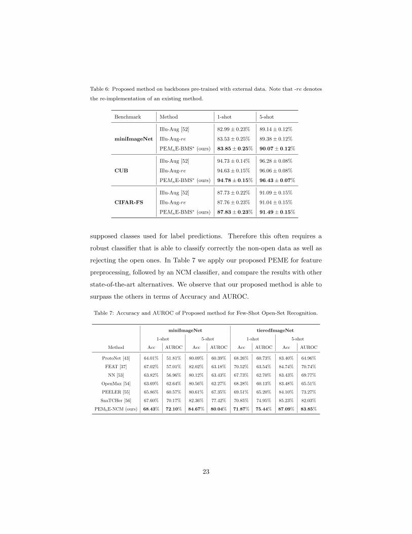
Table 6: Proposed method on backbones pre-trained with external data. Note that -re denotes

the re-implementation of an existing method.

Benchmark Method 1-shot 5-shot

miniImageNet

Illu-Aug [52] 82.99± 0.23% 89.14± 0.12%

Illu-Aug-re 83.53± 0.25% 89.38± 0.12%

PEMnE-BMS∗ (ours) 83.85± 0.25% 90.07± 0.12%

CUB

Illu-Aug [52] 94.73± 0.14% 96.28± 0.08%

Illu-Aug-re 94.63± 0.15% 96.06± 0.08%

PEMnE-BMS∗ (ours) 94.78± 0.15% 96.43± 0.07%

CIFAR-FS

Illu-Aug [52] 87.73± 0.22% 91.09± 0.15%

Illu-Aug-re 87.76± 0.23% 91.04± 0.15%

PEMnE-BMS∗ (ours) 87.83± 0.23% 91.49± 0.15%

supposed classes used for label predictions. Therefore this often requires a

robust classifier that is able to classify correctly the non-open data as well as

rejecting the open ones. In Table 7 we apply our proposed PEME for feature

preprocessing, followed by an NCM classifier, and compare the results with other

state-of-the-art alternatives. We observe that our proposed method is able to

surpass the others in terms of Accuracy and AUROC.

Table 7: Accuracy and AUROC of Proposed method for Few-Shot Open-Set Recognition.

miniImageNet tieredImageNet

1-shot 5-shot 1-shot 5-shot

Method Acc AUROC Acc AUROC Acc AUROC Acc AUROC

ProtoNet [43] 64.01% 51.81% 80.09% 60.39% 68.26% 60.73% 83.40% 64.96%

FEAT [37] 67.02% 57.01% 82.02% 63.18% 70.52% 63.54% 84.74% 70.74%

NN [53] 63.82% 56.96% 80.12% 63.43% 67.73% 62.70% 83.43% 69.77%

OpenMax [54] 63.69% 62.64% 80.56% 62.27% 68.28% 60.13% 83.48% 65.51%

PEELER [55] 65.86% 60.57% 80.61% 67.35% 69.51% 65.20% 84.10% 73.27%

SnaTCHer [56] 67.60% 70.17% 82.36% 77.42% 70.85% 74.95% 85.23% 82.03%

PEMbE-NCM (ours) 68.43% 72.10% 84.67% 80.04% 71.87% 75.44% 87.09% 83.85%

23

4.5. Proposed method on merged features

In this section we investigate the effect of our proposed method on merged

features. Namely, we perform a direct concatenation of raw feature vectors

extracted from multiple backbones at the beginning, followed by BMS. In

Table 8 we chose the feature vectors from three backbones (WRN, ResNet18

and ResNet12) and evaluated the performance with different combinations. We

observe that 1) a direct concatenation, depending on the backbones, can bring

about 1% gain in both 1-shot and 5-shot settings compared with the results

in Table 4 with feature vectors extracted from one single feature extractor. 2)

BMS∗ reached new state-of-the-art results on few-shot learning benchmarks with

feature vectors concatenated from WRN, ResNet18 and ResNet12, given that

no external data is used.

To further study the impact of the number of backbones on prediction

accuracy, in Figure 6 we depict the performance of our proposed method as a

function of the number of backbones. Note that here we operate on feature

vectors of 6 WRN backbones (dataset: miniImageNet) concatenated one after

another, which makes a total of 6 slots corresponding to a 640 × 6 = 3840

feature size. Each of them is trained the same way as in [7], and we randomly

select the multiples of 640 coordinates within the slots to denote the number

of concatenated backbones used. The performance result is the average of 100

random selections and we test with both BMS and BMS∗ for 1-shot, and BMS∗

for 5-shot. From Figure 6 we observe that, as the number of backbones increases,

there is a relatively steady growth in terms of accuracy in multiple settings of

our proposed method, indicating the interest of BMS in merged features.

5. Conclusion

In this paper we introduced a new pipeline to solve the few-shot classification

problem. Namely, we proposed to firstly preprocess the raw feature vectors

to better align to a Gaussian distribution and then we designed an optimal-

transport inspired iterative algorithm to estimate the class prototypes for the

24

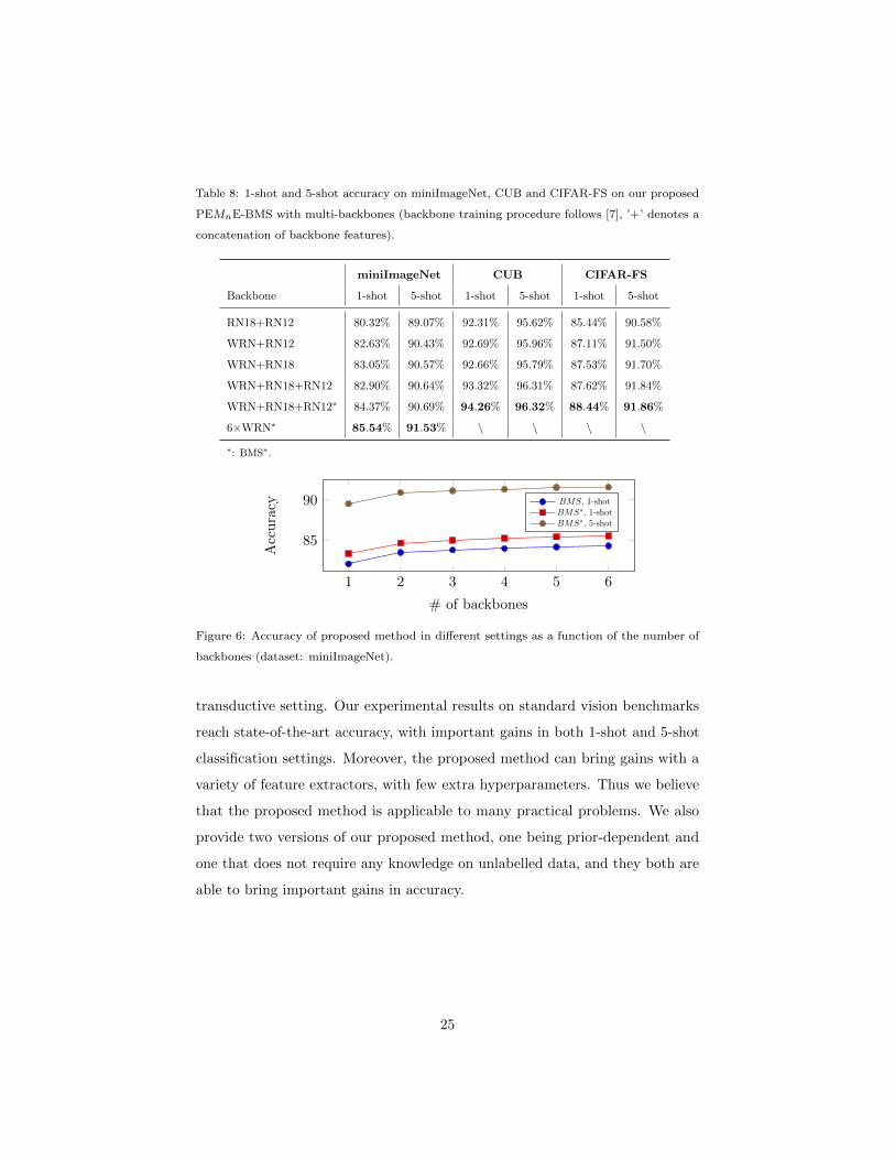
Table 8: 1-shot and 5-shot accuracy on miniImageNet, CUB and CIFAR-FS on our proposed

PEMnE-BMS with multi-backbones (backbone training procedure follows [7], ’+’ denotes a

concatenation of backbone features).

miniImageNet CUB CIFAR-FS

Backbone 1-shot 5-shot 1-shot 5-shot 1-shot 5-shot

RN18+RN12 80.32% 89.07% 92.31% 95.62% 85.44% 90.58%

WRN+RN12 82.63% 90.43% 92.69% 95.96% 87.11% 91.50%

WRN+RN18 83.05% 90.57% 92.66% 95.79% 87.53% 91.70%

WRN+RN18+RN12 82.90% 90.64% 93.32% 96.31% 87.62% 91.84%

WRN+RN18+RN12∗ 84.37% 90.69% 94.26% 96.32% 88.44% 91.86%

6×WRN∗ 85.54% 91.53% \ \ \ \

∗: BMS∗.

1 2 3 4 5 6

85

90

# of backbones

Acc

ura

cy BMS, 1-shotBMS∗, 1-shotBMS∗, 5-shot

Figure 6: Accuracy of proposed method in different settings as a function of the number of

backbones (dataset: miniImageNet).

transductive setting. Our experimental results on standard vision benchmarks

reach state-of-the-art accuracy, with important gains in both 1-shot and 5-shot

classification settings. Moreover, the proposed method can bring gains with a

variety of feature extractors, with few extra hyperparameters. Thus we believe

that the proposed method is applicable to many practical problems. We also

provide two versions of our proposed method, one being prior-dependent and

one that does not require any knowledge on unlabelled data, and they both are

able to bring important gains in accuracy.

25

References

[1] C. Finn, P. Abbeel, S. Levine, Model-agnostic meta-learning for fast adapta-

tion of deep networks, in: Proceedings of the 34th International Conference

on Machine Learning-Volume 70, JMLR. org, 2017, pp. 1126–1135.

[2] S. Ravi, H. Larochelle, Optimization as a model for few-shot learning, in: 5th

International Conference on Learning Representations, ICLR 2017, Toulon,

France, April 24-26, 2017, Conference Track Proceedings, OpenReview.net,

2017.

URL https://openreview.net/forum?id=rJY0-Kcll

[3] S. Thrun, L. Pratt, Learning to learn, Springer Science & Business Media,

2012.

[4] L. Torrey, J. Shavlik, Transfer learning, in: Handbook of research on machine

learning applications and trends: algorithms, methods, and techniques, IGI

Global, 2010, pp. 242–264.

[5] D. Das, C. S. G. Lee, A two-stage approach to few-shot learning for image

recognition, IEEE Trans. Image Process. 29 (2020) 3336–3350. doi:10.

1109/TIP.2019.2959254.

URL https://doi.org/10.1109/TIP.2019.2959254

[6] W. Chen, Y. Liu, Z. Kira, Y. F. Wang, J. Huang, A closer look at few-shot

classification, in: 7th International Conference on Learning Representations,

ICLR 2019, New Orleans, LA, USA, May 6-9, 2019, OpenReview.net, 2019.

URL https://openreview.net/forum?id=HkxLXnAcFQ

[7] P. Mangla, N. Kumari, A. Sinha, M. Singh, B. Krishnamurthy, V. N.

Balasubramanian, Charting the right manifold: Manifold mixup for few-

shot learning, in: The IEEE Winter Conference on Applications of Computer

Vision, 2020, pp. 2218–2227.

26

[8] Y. Hu, V. Gripon, S. Pateux, Graph-based interpolation of feature vectors

for accurate few-shot classification, in: 2020 25th International Conference

on Pattern Recognition (ICPR), IEEE, 2021, pp. 8164–8171.

[9] Y. Hu, V. Gripon, S. Pateux, Leveraging the feature distribution in transfer-

based few-shot learning, in: International Conference on Artificial Neural

Networks, Springer, 2021, pp. 487–499.

[10] Z. Li, F. Zhou, F. Chen, H. Li, Meta-sgd: Learning to learn quickly for few

shot learning, CoRR abs/1707.09835. arXiv:1707.09835.

URL http://arxiv.org/abs/1707.09835

[11] A. Antoniou, H. Edwards, A. J. Storkey, How to train your MAML, in: 7th

International Conference on Learning Representations, ICLR 2019, New

Orleans, LA, USA, May 6-9, 2019, OpenReview.net, 2019.

URL https://openreview.net/forum?id=HJGven05Y7

[12] L. Bertinetto, J. F. Henriques, P. H. S. Torr, A. Vedaldi, Meta-learning

with differentiable closed-form solvers, in: 7th International Conference on

Learning Representations, ICLR 2019, New Orleans, LA, USA, May 6-9,

2019, OpenReview.net, 2019.

URL https://openreview.net/forum?id=HyxnZh0ct7

[13] H. Zhang, J. Zhang, P. Koniusz, Few-shot learning via saliency-guided hal-

lucination of samples, in: Proceedings of the IEEE Conference on Computer

Vision and Pattern Recognition, 2019, pp. 2770–2779.

[14] Z. Chen, Y. Fu, Y.-X. Wang, L. Ma, W. Liu, M. Hebert, Image deformation

meta-networks for one-shot learning, in: Proceedings of the IEEE Conference

on Computer Vision and Pattern Recognition, 2019, pp. 8680–8689.

[15] T. Mensink, J. Verbeek, F. Perronnin, G. Csurka, Metric learning for large

scale image classification: Generalizing to new classes at near-zero cost, in:

European Conference on Computer Vision, Springer, 2012, pp. 488–501.

27

[16] O. Chapelle, B. Scholkopf, A. Zien, Semi-supervised learning (chapelle, o.

et al., eds.; 2006)[book reviews], IEEE Transactions on Neural Networks

20 (3) (2009) 542–542.

[17] Y. Wang, W. Chao, K. Q. Weinberger, L. van der Maaten, Simpleshot:

Revisiting nearest-neighbor classification for few-shot learning, CoRR

abs/1911.04623. arXiv:1911.04623.

URL http://arxiv.org/abs/1911.04623

[18] M. Lichtenstein, P. Sattigeri, R. Feris, R. Giryes, L. Karlinsky, Tafssl: Task-

adaptive feature sub-space learning for few-shot classification, in: European

Conference on Computer Vision, Springer, 2020, pp. 522–539.

[19] V. Gripon, G. B. Hacene, M. Lowe, F. Vermet, Improving accuracy of non-

parametric transfer learning via vector segmentation, in: 2018 IEEE Inter-

national Conference on Acoustics, Speech and Signal Processing (ICASSP),

2018, pp. 2966–2970.

[20] S. Yang, L. Liu, M. Xu, Free lunch for few-shot learning: Distribution

calibration, in: 9th International Conference on Learning Representations,

ICLR 2021, Virtual Event, Austria, May 3-7, 2021, OpenReview.net, 2021.

URL https://openreview.net/forum?id=JWOiYxMG92s

[21] Y. Liu, J. Lee, M. Park, S. Kim, E. Yang, S. J. Hwang, Y. Yang, Learning to

propagate labels: Transductive propagation network for few-shot learning,

in: 7th International Conference on Learning Representations, ICLR 2019,

New Orleans, LA, USA, May 6-9, 2019, OpenReview.net, 2019.

URL https://openreview.net/forum?id=SyVuRiC5K7

[22] A. F. Agarap, Deep learning using rectified linear units (relu), CoRR

abs/1803.08375. arXiv:1803.08375.

URL http://arxiv.org/abs/1803.08375

[23] J. W. Tukey, Exploratory data analysis, Vol. 2, Reading, Mass., 1977.

28

[24] R. G. Cinbis, J. Verbeek, C. Schmid, Approximate fisher kernels of non-

iid image models for image categorization, IEEE transactions on pattern

analysis and machine intelligence 38 (6) (2015) 1084–1098.

[25] C. Villani, Optimal transport: old and new, Vol. 338, Springer Science &

Business Media, 2008.

[26] M. Cuturi, Sinkhorn distances: Lightspeed computation of optimal trans-

port, in: Advances in neural information processing systems, 2013, pp.

2292–2300.

[27] J. Solomon, F. De Goes, G. Peyre, M. Cuturi, A. Butscher, A. Nguyen,

T. Du, L. Guibas, Convolutional wasserstein distances: Efficient optimal

transportation on geometric domains, ACM Transactions on Graphics

(TOG) 34 (4) (2015) 1–11.

[28] A. P. Dempster, N. M. Laird, D. B. Rubin, Maximum likelihood from

incomplete data via the em algorithm, Journal of the Royal Statistical

Society: Series B (Methodological) 39 (1) (1977) 1–22.

[29] O. Vinyals, C. Blundell, T. Lillicrap, D. Wierstra, et al., Matching networks

for one shot learning, in: Advances in neural information processing systems,

2016, pp. 3630–3638.

[30] M. Ren, E. Triantafillou, S. Ravi, J. Snell, K. Swersky, J. B. Tenenbaum,

H. Larochelle, R. S. Zemel, Meta-learning for semi-supervised few-shot

classification, in: 6th International Conference on Learning Representations,

ICLR 2018, Vancouver, BC, Canada, April 30 - May 3, 2018, Conference

Track Proceedings, OpenReview.net, 2018.

URL https://openreview.net/forum?id=HJcSzz-CZ

[31] C. Wah, S. Branson, P. Welinder, P. Perona, S. Belongie, The Caltech-UCSD

Birds-200-2011 Dataset, Tech. Rep. CNS-TR-2011-001, California Institute

of Technology (2011).

29

[32] O. Russakovsky, J. Deng, H. Su, J. Krause, S. Satheesh, S. Ma, Z. Huang,

A. Karpathy, A. Khosla, M. Bernstein, et al., Imagenet large scale visual

recognition challenge, International journal of computer vision 115 (3) (2015)

211–252.

[33] S. Zagoruyko, N. Komodakis, Wide residual networks, in: R. C. Wilson,

E. R. Hancock, W. A. P. Smith (Eds.), Proceedings of the British Machine

Vision Conference 2016, BMVC 2016, York, UK, September 19-22, 2016,

BMVA Press, 2016.

URL http://www.bmva.org/bmvc/2016/papers/paper087/index.html

[34] K. He, X. Zhang, S. Ren, J. Sun, Deep residual learning for image recognition,

in: Proceedings of the IEEE conference on computer vision and pattern

recognition, 2016, pp. 770–778.

[35] G. Huang, Z. Liu, L. Van Der Maaten, K. Q. Weinberger, Densely connected

convolutional networks, in: Proceedings of the IEEE conference on computer

vision and pattern recognition, 2017, pp. 4700–4708.

[36] C. Zhang, Y. Cai, G. Lin, C. Shen, Deepemd: Few-shot image classification

with differentiable earth mover’s distance and structured classifiers, in:

Proceedings of the IEEE/CVF conference on computer vision and pattern

recognition, 2020, pp. 12203–12213.

[37] H.-J. Ye, H. Hu, D.-C. Zhan, F. Sha, Few-shot learning via embedding

adaptation with set-to-set functions, in: Proceedings of the IEEE/CVF

Conference on Computer Vision and Pattern Recognition, 2020, pp. 8808–

8817.

[38] J. Liu, L. Song, Y. Qin, Prototype rectification for few-shot learning, in:

Computer Vision–ECCV 2020: 16th European Conference, Glasgow, UK,

August 23–28, 2020, Proceedings, Part I 16, Springer, 2020, pp. 741–756.

[39] I. Ziko, J. Dolz, E. Granger, I. B. Ayed, Laplacian regularized few-shot

30

learning, in: International Conference on Machine Learning, PMLR, 2020,

pp. 11660–11670.

[40] M. Boudiaf, I. M. Ziko, J. Rony, J. Dolz, P. Piantanida, I. B. Ayed, Transduc-

tive information maximization for few-shot learning, CoRR abs/2008.11297.

arXiv:2008.11297.

URL https://arxiv.org/abs/2008.11297

[41] S. M. Kye, H. Lee, H. Kim, S. J. Hwang, Transductive few-shot learning

with meta-learned confidence, CoRR abs/2002.12017. arXiv:2002.12017.

URL https://arxiv.org/abs/2002.12017

[42] P. Rodrıguez, I. Laradji, A. Drouin, A. Lacoste, Embedding propagation:

Smoother manifold for few-shot classification, in: European Conference on

Computer Vision, Springer, 2020, pp. 121–138.

[43] J. Snell, K. Swersky, R. Zemel, Prototypical networks for few-shot learning,

in: Advances in Neural Information Processing Systems, 2017, pp. 4077–

4087.

[44] A. A. Rusu, D. Rao, J. Sygnowski, O. Vinyals, R. Pascanu, S. Osindero,

R. Hadsell, Meta-learning with latent embedding optimization, in: 7th

International Conference on Learning Representations, ICLR 2019, New

Orleans, LA, USA, May 6-9, 2019, OpenReview.net, 2019.

URL https://openreview.net/forum?id=BJgklhAcK7

[45] D. Kang, H. Kwon, J. Min, M. Cho, Relational embedding for few-shot

classification, CoRR abs/2108.09666. arXiv:2108.09666.

URL https://arxiv.org/abs/2108.09666

[46] T. Chobola, D. Vasata, P. Kordık, Transfer learning based few-shot classifi-

cation using optimal transport mapping from preprocessed latent space of

backbone neural network, CoRR abs/2102.05176. arXiv:2102.05176.

URL https://arxiv.org/abs/2102.05176

31

[47] C. Simon, P. Koniusz, R. Nock, M. Harandi, Adaptive subspaces for few-shot

learning, in: Proceedings of the IEEE/CVF Conference on Computer Vision

and Pattern Recognition, 2020, pp. 4136–4145.

[48] V. Verma, A. Lamb, C. Beckham, A. Najafi, I. Mitliagkas, D. Lopez-Paz,

Y. Bengio, Manifold mixup: Better representations by interpolating hidden

states, in: International Conference on Machine Learning, PMLR, 2019, pp.

6438–6447.

[49] S. Ioffe, C. Szegedy, Batch normalization: Accelerating deep network train-

ing by reducing internal covariate shift, in: International conference on

machine learning, PMLR, 2015, pp. 448–456.

[50] R. DIAgostino, An omnibus test of normality for moderate and large sample

sizes, Biometrika 58 (34) (1971) 1–348.

[51] R. D’AGOSTINO, E. S. Pearson, Tests for departure from normality. em-

pirical results for the distributions of b 2 and√b, Biometrika 60 (3) (1973)

613–622.

[52] H. Zhang, Z. Cao, Z. Yan, C. Zhang, Sill-net: Feature augmentation with

separated illumination representation, CoRR abs/2102.03539. arXiv:2102.

03539.

URL https://arxiv.org/abs/2102.03539

[53] P. R. M. Junior, R. M. De Souza, R. d. O. Werneck, B. V. Stein, D. V.

Pazinato, W. R. de Almeida, O. A. Penatti, R. d. S. Torres, A. Rocha,

Nearest neighbors distance ratio open-set classifier, Machine Learning 106 (3)

(2017) 359–386.

[54] A. Bendale, T. E. Boult, Towards open set deep networks, in: Proceedings

of the IEEE conference on computer vision and pattern recognition, 2016,

pp. 1563–1572.

32

[55] B. Liu, H. Kang, H. Li, G. Hua, N. Vasconcelos, Few-shot open-set recogni-

tion using meta-learning, in: Proceedings of the IEEE/CVF Conference on

Computer Vision and Pattern Recognition, 2020, pp. 8798–8807.

[56] M. Jeong, S. Choi, C. Kim, Few-shot open-set recognition by transformation

consistency, in: Proceedings of the IEEE/CVF Conference on Computer

Vision and Pattern Recognition, 2021, pp. 12566–12575.

33