The Orange Crush: The Squeezing of Orange County's Middle ... · The Orange Crush: The Squeezing of Orange County's Middle Class 1 John R. Hipp* January 28, 2009 ... The Squeezing

The Orange Crush: The Squeezing of Orange County's Middle Class 1

John R. Hipp*

January 28, 2009 * Department of Criminology, Law and Society and Department of Sociology, University of California, Irvine. Address correspondence to John R. Hipp, Department of Criminology, Law and Society, University of California, Irvine, 2367 Social Ecology II, Irvine, CA 92697; email: [email protected]. 1 Special thanks to Scott Smith and Dan Yates for creating the maps in this report.

The Orange Crush: The Squeezing of Orange County's Middle Class

The Orange Crush: The Squeezing of Orange County's Middle Class Summary

Exploring data over a thirty year period, this study documents the demographic

and economic changes in Orange County over that period. Orange County has grown dramatically since its days as a basin for the Valencia Orange—both in population and geography. There has been a boom of growth since the post WWII days of 1940. The bulk of the growth has taken place since the beginning of 1970, with the population more than doubling in size.

Many people came here to buy a home and find a good-paying job—in short—to realize the American Dream. However, over the past 35 years, that realization has become much less attainable due to policies that have shaped Orange County into an hourglass economy.

• Most housing is no longer affordable to low- and middle-income families. The cost of housing in Orange County remains among the highest in the nation

• Orange County’s population continues to increase, but affordable jobs are becoming harder to find. The jobs with the most openings are low-skilled and low-paying.

ii


Table of Contents List of Figures ................................................................................................................ iv List of Tables ................................................................................................................. iv

Chapter 1. Introduction to the Problems and Challenges .................................................. 1 Chapter 2. The change in Orange County over time ......................................................... 3

Racial/ethnic transformation........................................................................................... 5 Poverty .......................................................................................................................... 13

Chapter 3: The Economy .................................................................................................. 15 Income and inequality................................................................................................... 15 Labor market characteristics ......................................................................................... 21 Working Poverty........................................................................................................... 25

Chapter 4. Housing and the cost of living........................................................................ 26 Chapter 5. What we have learned, and future directions ................................................. 32

Policy implications........................................................................................................ 33 What government should do: .................................................................................... 33 What Business should do:......................................................................................... 34 What Community and Labor should do:................................................................... 35

References......................................................................................................................... 36 Appendix........................................................................................................................... 37

iii


List of Figures

Figure 2.1 Population growth in Orange County from 1940 to 2000................................. 3 Figure 2.2 Ratio of population density in Orange County to average U.S. County ........... 4 from 1940 to 2000............................................................................................................... 4 Figure 2.3 Total population by city, 2000........................................................................... 5 Figure 2.4 Percent white in Orange County and the U.S. from 1970 to 2000.................... 6 Figure 2.5 Percent white by city, 2000 .............................................................................. 7 Figure 2.6 Map of percent white residents in census tracts, 2000 ...................................... 8 Figure 2.7 Percent Latino in Orange County and the U.S. from 1970 to 2000 ................. 9 Figure 2.8 Racial/ethnic heterogeneity in Orange County and the U.S. from 1970 to 2000

................................................................................................................................... 10 Figure 2.9 Change in racial/ethnic heterogeneity by city, 1970-2000.............................. 11 Figure 2.10 Map of racial/ethnic heterogeneity in census tracts, 2000 ............................ 12 Figure 2.11 Percent in poverty in Orange County and the U.S. from 1970 to 2000 ........ 13 Figure 2.12 Percent in poverty by city, 2000.................................................................... 14 Figure 3.1 Median household income (in real 1983 dollars) in Orange County and the

U.S. from 1970 to 2000............................................................................................. 16 Figure 3.2 Real average family income in 1982 dollars by city, 2000 ............................. 17 Figure 3.3 Change in real average family income by city, 1970-2000............................. 18 Figure 3.4 Family income inequality (Gini coefficient) in Orange County and the U.S. 19 from 1970 to 2000............................................................................................................. 19 Figure 3.5 Share of the Pie: Distribution of Aggregate Income by Quintile .................... 19 Figure 3.6 Inequality in family income (Gini coefficient) by city, 2000.......................... 20 Figure 3.7 Change in inequality in family income by city, 1970-2000 ............................ 21 Figure 3.8 Unemployment rate in Orange County and the U.S. from 1970 to 2000........ 21 Figure 3.9 Percent unemployed by city, 2000 .................................................................. 22 Figure 3.10 Educational achievement distribution in Orange County and the U.S.......... 23 from 1970 to 2000............................................................................................................. 23 Figure 3.11 Percent with at least a bachelor’s degree by city, 2000................................. 24 Figure 4.1 Median rent (in real 1983 dollars) in Orange County and the U.S.................. 26 from 1970 to 2000............................................................................................................. 26 Figure 4.2 Median home value (in real 1983 dollars) in Orange County and the U.S. .... 27 from 1970 to 2000............................................................................................................. 27 Figure 4.3 Map of average home values in census tracts, 2000 ....................................... 28 Figure 4.4 Map of change in average home values in census tracts, 1970-2000.............. 30 Figure 4.5 Ratio of Orange County to average U.S. County values for median household

income, rent and home values (in real 1983 dollars) from 1970 to 2000 ................. 31 List of Tables

Table 3.1 Occupations with the most job openings, 2004 – 2014, Orange County……. 36

iv


Chapter 1. Introduction to the Problems and Challenges From all appearances, Orange County is indeed Paradise Found. From its roots as a rural farming paradise specializing first in grape crops and later in crops of Valencia oranges, to its post-World War II population boom and accompanying economic boom, there would apparently be few blemishes on the trajectory of this “boomburb.” The land of fun and sun, and the fantasyland that gave birth to Disneyland, surely this must be paradise. A rough-hewn frontier where individuals made their way to find their dreams in the land of movies, the area has long been characterized by an individualistic ethos. As we detail in this report, the numbers are staggering. The population has experienced a 20-fold increase in 60 years. Home values are among the highest in the nation, as the median home value in Orange County has remained among the top 1% of U.S. counties since 1970. It is a land of plenty, as the median real household income in Orange County is about 50% higher than the average U.S. County. At least one component of the work force is very well trained, as nearly 1/3 of the county residents have at least a bachelor’s degree, nearly double the rate of the average U.S. County. Nonetheless, despite all these positive features, there appear to be cracks in the façade that suggest perhaps this paradise may be a mirage, or perhaps even lost. As we illustrate in this report, there are signs of growing inequality in the county. This inequality is accompanied by evidence of a bifurcating labor force in which the middle-class blue-collar worker appears to be an endangered species. Accompanying this is the evidence that real income levels have not kept pace with the appreciation in real costs of homes and rents, resulting in a more challenging cost of living environment. We provide a socio-demographic description of Orange County over the 30-year period of 1970 to 2000 (and in some instances provide data for 2006). In some instances, we provide information on the changes in the county over the last 60 years. We map the growing levels of inequality in the county. This report focuses on three broad areas: 1) illustrating the socio-demographic changes in the county; 2) mapping the state of the economy; 3) detailing the cost of living and the cost of housing in the county. Three broad trends can be detected in the county over this period: 1) the County has undergone an enormous racial/ethnic transition from a homogenous 88% white community in 1970, to nearly 50% nonwhite in 2000, with a large percentage of that change coming from Latinos. The Latino population increased from 12% in 1970 to 31% in 2000, and in immigrants from about 5% in 1970 to 30% in 2000. 2) the County has seen a general increase in economic inequality, as the percentage in poverty has increased, the cost of living has worsened as the median income relative to the rest of the U.S. has held flat while rents and home values have increased considerably relative to the rest of the U.S. 3) a changing educational composition of the workforce as the increasing percentage with a bachelor’s degree is accompanied by a stubbornly constant percentage with less than a high

1


school degree, and as a consequence the percentage with a high school degree that have not gone on to college—the middle-class blue collar segment—is shrinking.

In this report, we will first look at the changes in Orange County over the past 35 years. We will then examine the economy and inequality in Orange County as it relates to jobs and the wages that are being produced in Orange County’s regional economy. Next we will examine housing affordability, the impact of growth on quality of life in the OC. Lastly, we review policy approaches that can generate more sustainable growth for Orange County’s future.

2


Chapter 2. The change in Orange County over time

In the chapter, we describe how Orange County has changed over the last 30 to 60 years.

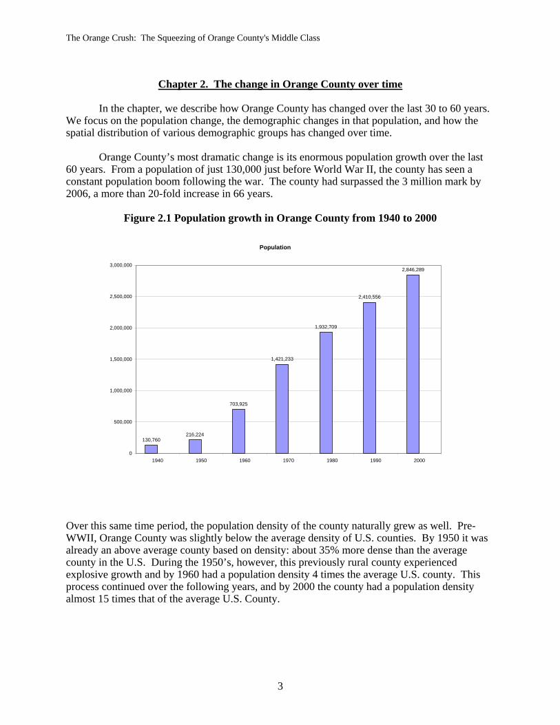
We focus on the population change, the demographic changes in that population, and how the spatial distribution of various demographic groups has changed over time. Orange County’s most dramatic change is its enormous population growth over the last 60 years. From a population of just 130,000 just before World War II, the county has seen a constant population boom following the war. The county had surpassed the 3 million mark by 2006, a more than 20-fold increase in 66 years.

Figure 2.1 Population growth in Orange County from 1940 to 2000

ver this same time period, the population density of the county naturally grew as well. Pre-as

his

Population

130,760216,224

703,925

1,421,233

1,932,709

2,410,556

2,846,289

0

500,000

1,000,000

1,500,000

2,000,000

2,500,000

3,000,000

1940 1950 1960 1970 1980 1990 2000

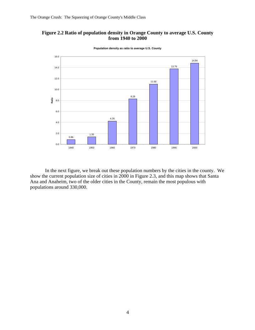
OWWII, Orange County was slightly below the average density of U.S. counties. By 1950 it walready an above average county based on density: about 35% more dense than the average county in the U.S. During the 1950’s, however, this previously rural county experienced explosive growth and by 1960 had a population density 4 times the average U.S. county. Tprocess continued over the following years, and by 2000 the county had a population density almost 15 times that of the average U.S. County.

3


Figure 2.2 Ratio of population density in Orange County to average U.S. County

In the next figure, we break out these population numbers by the cities in the county. We show th

from 1940 to 2000

Population density as ratio to average U.S. County

0.861.35

4.26

8.28

11.00

13.76

14.84

0.0

2.0

4.0

6.0

8.0

10.0

12.0

14.0

16.0

1940 1950 1960 1970 1980 1990 2000

Rat

io

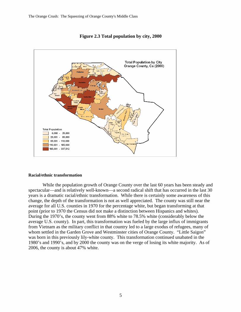
e current population size of cities in 2000 in Figure 2.3, and this map shows that Santa Ana and Anaheim, two of the older cities in the County, remain the most populous with populations around 330,000.

4


Figure 2.3 Total population by city, 2000

acial/ethnic transformation

While the population growth of Orange County over the last 60 years has been steady and

s

f

R

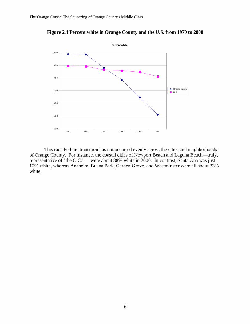
spectacular—and is relatively well-known—a second radical shift that has occurred in the last 30 years is a dramatic racial/ethnic transformation. While there is certainly some awareness of this change, the depth of the transformation is not as well appreciated. The county was still near the average for all U.S. counties in 1970 for the percentage white, but began transforming at that point (prior to 1970 the Census did not make a distinction between Hispanics and whites). During the 1970’s, the county went from 88% white to 78.5% white (considerably below theaverage U.S. county). In part, this transformation was fueled by the large influx of immigrantfrom Vietnam as the military conflict in that country led to a large exodus of refugees, many of whom settled in the Garden Grove and Westminster cities of Orange County. “Little Saigon” was born in this previously lily-white county. This transformation continued unabated in the 1980’s and 1990’s, and by 2000 the county was on the verge of losing its white majority. As o2006, the county is about 47% white.

5


Figure 2.4 Percent white in Orange County and the U.S. from 1970 to 2000

This racial/ethnic transition has not occurred evenly across the cities and neighborhoods f Orange County. For instance, the coastal cities of Newport Beach and Laguna Beach—truly, prese

Percent white

40.0

50.0

60.0

70.0

80.0

90.0

100.0

1950 1960 1970 1980 1990 2000

Orange CountyU.S.

ore ntative of “the O.C.”— were about 88% white in 2000. In contrast, Santa Ana was just 12% white, whereas Anaheim, Buena Park, Garden Grove, and Westminster were all about 33% white.

6


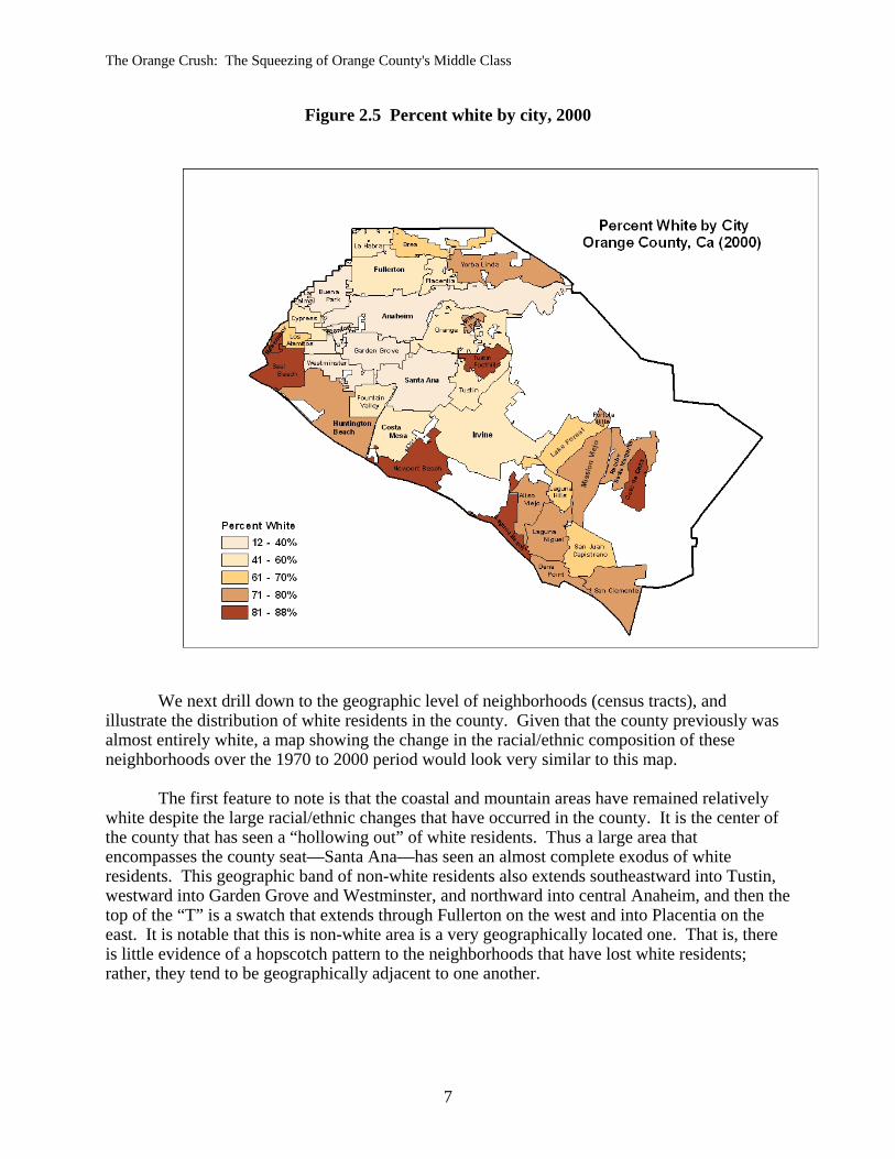
Figure 2.5 Percent white by city, 2000

We next drill down to the geographic level of neighborhoods (census tracts), and

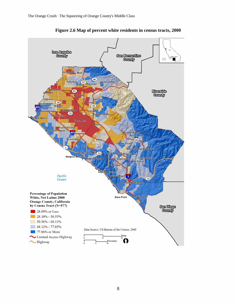
illustrate the distribution of white residents in the county. Given that the county previously was almost entirely white, a map showing the change in the racial/ethnic composition of these neighborhoods over the 1970 to 2000 period would look very similar to this map.

The first feature to note is that the coastal and mountain areas have remained relatively

white despite the large racial/ethnic changes that have occurred in the county. It is the center of the county that has seen a “hollowing out” of white residents. Thus a large area that encompasses the county seat—Santa Ana—has seen an almost complete exodus of white residents. This geographic band of non-white residents also extends southeastward into Tustin, westward into Garden Grove and Westminster, and northward into central Anaheim, and then the top of the “T” is a swatch that extends through Fullerton on the west and into Placentia on the east. It is notable that this is non-white area is a very geographically located one. That is, there is little evidence of a hopscotch pattern to the neighborhoods that have lost white residents; rather, they tend to be geographically adjacent to one another.

7


Figure 2.6 Map of percent white residents in census tracts, 2000

8


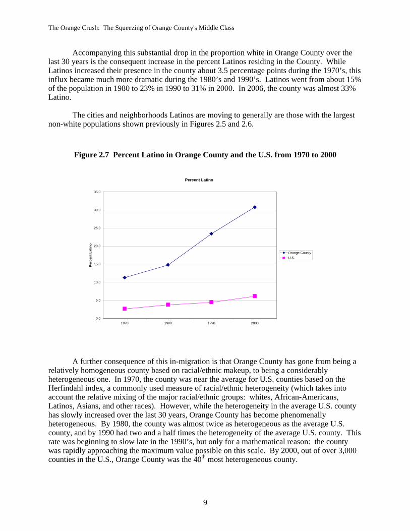
Accompanying this substantial drop in the proportion white in Orange County over the last 30 years is the consequent increase in the percent Latinos residing in the County. While Latinos increased their presence in the county about 3.5 percentage points during the 1970’s, this influx became much more dramatic during the 1980’s and 1990’s. Latinos went from about 15% of the population in 1980 to 23% in 1990 to 31% in 2000. In 2006, the county was almost 33% Latino.

The cities and neighborhoods Latinos are moving to generally are those with the largest

non-white populations shown previously in Figures 2.5 and 2.6.

Figure 2.7 Percent Latino in Orange County and the U.S. from 1970 to 2000

Percent Latino

0.0

5.0

10.0

15.0

20.0

25.0

30.0

35.0

1970 1980 1990 2000

Perc

ent L

atin

o

Orange CountyU.S.

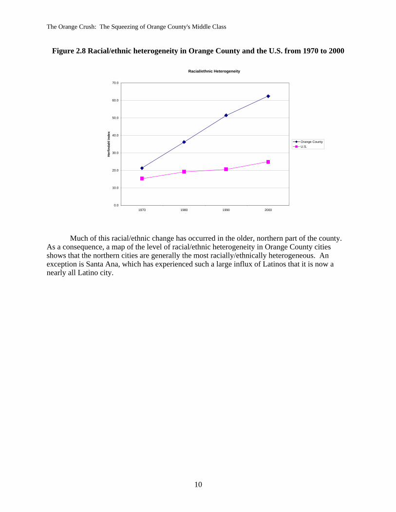
A further consequence of this in-migration is that Orange County has gone from being a relatively homogeneous county based on racial/ethnic makeup, to being a considerably heterogeneous one. In 1970, the county was near the average for U.S. counties based on the Herfindahl index, a commonly used measure of racial/ethnic heterogeneity (which takes into account the relative mixing of the major racial/ethnic groups: whites, African-Americans, Latinos, Asians, and other races). However, while the heterogeneity in the average U.S. county has slowly increased over the last 30 years, Orange County has become phenomenally heterogeneous. By 1980, the county was almost twice as heterogeneous as the average U.S. county, and by 1990 had two and a half times the heterogeneity of the average U.S. county. This rate was beginning to slow late in the 1990’s, but only for a mathematical reason: the county was rapidly approaching the maximum value possible on this scale. By 2000, out of over 3,000 counties in the U.S., Orange County was the 40th most heterogeneous county.

9


Figure 2.8 Racial/ethnic heterogeneity in Orange County and the U.S. from 1970 to 2000

Much of this racial/ethnic change has occurred in the older, northern part of the county.

Racial/ethnic Heterogeneity

0.0

10.0

20.0

30.0

40.0

50.0

60.0

70.0

1970 1980 1990 2000

Her

finda

hl in

dex

Orange CountyU.S.

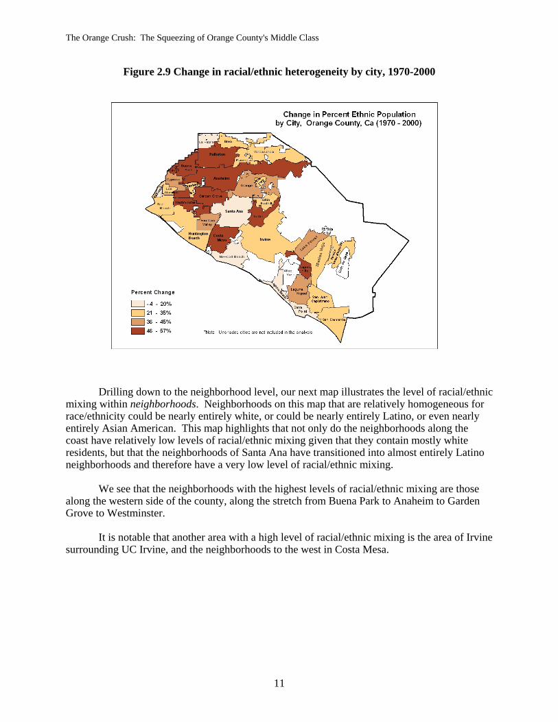
As a consequence, a map of the level of racial/ethnic heterogeneity in Orange County cities shows that the northern cities are generally the most racially/ethnically heterogeneous. An exception is Santa Ana, which has experienced such a large influx of Latinos that it is now anearly all Latino city.

10


Figure 2.9 Change in racial/ethnic heterogeneity by city, 1970-2000

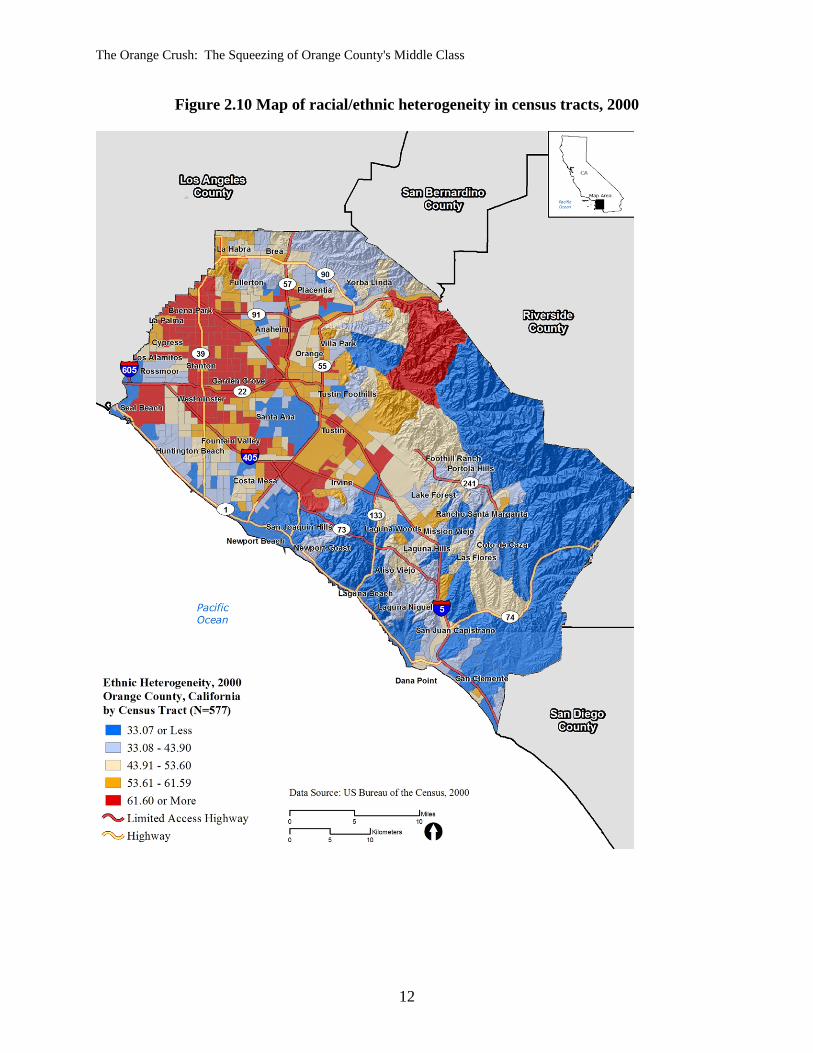
rilling down to the neighborhood level, our next map illustrates the level of racial/ethnic

mixing

no

mixing are those

nother area with a high level of racial/ethnic mixing is the area of Irvine

D within neighborhoods. Neighborhoods on this map that are relatively homogeneous for

race/ethnicity could be nearly entirely white, or could be nearly entirely Latino, or even nearly entirely Asian American. This map highlights that not only do the neighborhoods along the coast have relatively low levels of racial/ethnic mixing given that they contain mostly white residents, but that the neighborhoods of Santa Ana have transitioned into almost entirely Latineighborhoods and therefore have a very low level of racial/ethnic mixing.

We see that the neighborhoods with the highest levels of racial/ethnic along the western side of the county, along the stretch from Buena Park to Anaheim to Garden Grove to Westminster.

It is notable that a surrounding UC Irvine, and the neighborhoods to the west in Costa Mesa.

11


Figure 2.10 Map of racial/ethnic heterogeneity in census tracts, 2000

12


Poverty

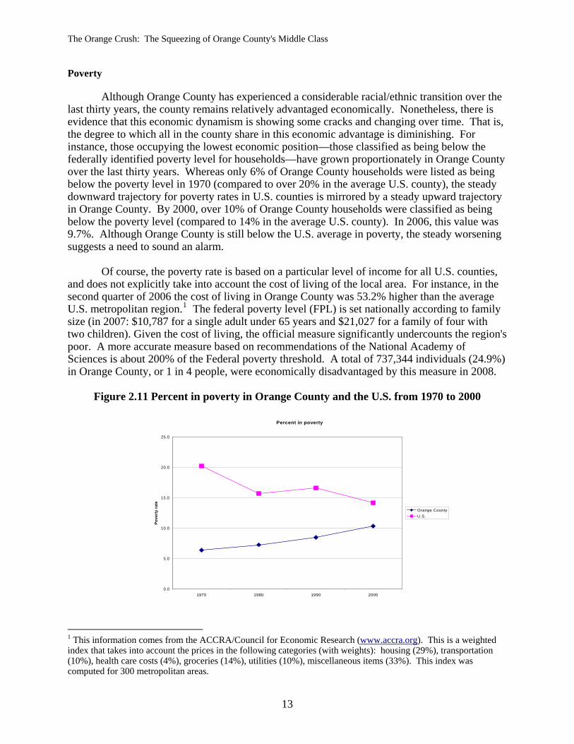
Although Orange County has experienced a considerable racial/ethnic transition over the last thirty years, the county remains relatively advantaged economically. Nonetheless, there is evidence that this economic dynamism is showing some cracks and changing over time. That is, the degree to which all in the county share in this economic advantage is diminishing. For instance, those occupying the lowest economic position—those classified as being below the federally identified poverty level for households—have grown proportionately in Orange County over the last thirty years. Whereas only 6% of Orange County households were listed as being below the poverty level in 1970 (compared to over 20% in the average U.S. county), the steady downward trajectory for poverty rates in U.S. counties is mirrored by a steady upward trajectory in Orange County. By 2000, over 10% of Orange County households were classified as being below the poverty level (compared to 14% in the average U.S. county). In 2006, this value was 9.7%. Although Orange County is still below the U.S. average in poverty, the steady worsening suggests a need to sound an alarm.

Of course, the poverty rate is based on a particular level of income for all U.S. counties,

and does not explicitly take into account the cost of living of the local area. For instance, in the second quarter of 2006 the cost of living in Orange County was 53.2% higher than the average U.S. metropolitan region.1 The federal poverty level (FPL) is set nationally according to family size (in 2007: $10,787 for a single adult under 65 years and $21,027 for a family of four with two children). Given the cost of living, the official measure significantly undercounts the region's poor. A more accurate measure based on recommendations of the National Academy of Sciences is about 200% of the Federal poverty threshold. A total of 737,344 individuals (24.9%) in Orange County, or 1 in 4 people, were economically disadvantaged by this measure in 2008.

Figure 2.11 Percent in poverty in Orange County and the U.S. from 1970 to 2000

Percent in poverty

0.0

5.0

10.0

15.0

20.0

25.0

1970 1980 1990 2000

Pove

rty

rate

Orange CountyU.S.

1 This information comes from the ACCRA/Council for Economic Research (www.accra.org). This is a weighted index that takes into account the prices in the following categories (with weights): housing (29%), transportation (10%), health care costs (4%), groceries (14%), utilities (10%), miscellaneous items (33%). This index was computed for 300 metropolitan areas.

13

http://www.accra.org/


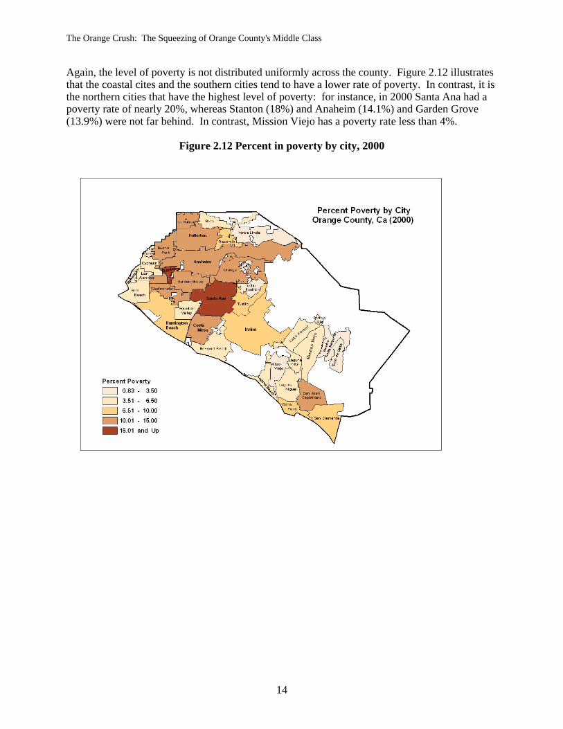
Again, the level of poverty is not distributed uniformly across the county. Figure 2.12 illustrates that the coastal cites and the southern cities tend to have a lower rate of poverty. In contrast, it is the northern cities that have the highest level of poverty: for instance, in 2000 Santa Ana had a poverty rate of nearly 20%, whereas Stanton (18%) and Anaheim (14.1%) and Garden Grove (13.9%) were not far behind. In contrast, Mission Viejo has a poverty rate less than 4%.

Figure 2.12 Percent in poverty by city, 2000

14


Chapter 3: The Economy

In this chapter, we focus on the economy of Orange County. We ask how households are doing economically over this time period on average, and we also ask whether differences are observed for those at different ends of the economic spectrum. Specifically, we focus on the growth in inequality over this time period in the county. We describe how this inequality is geographically disbursed throughout the county. Although the levels of unemployment in the county have traditionally been relatively low, we show how these are growing in recent years, as well as how this unemployment is not spread evenly across the geographic landscape of the county.

We also point out that while part of the labor force in Orange County is highly educated,

there is evidence of an increasingly bimodal distribution in which there is also relative growth in those with the lowest levels of education. This portends a challenge to the economy of the county to maintain quality blue collar jobs. The loss of such jobs would likely only exacerbate the already growing inequality.

This chapter will also document the negative consequences of growth in low-wage

industries and the tools we have at our disposal to foster positive economic development. The high cost of living is in contrast to the low-wage service sector economy that has emerged. This chapter tracks the trends in Orange County, dating back to 1970, that have shaped our current economy. We will examine the kinds of jobs that have been created in the midst of Orange County’s phenomenal growth, as well as assess the impact of job quality on the long-term sustainability of our regional economy.

Income and inequality

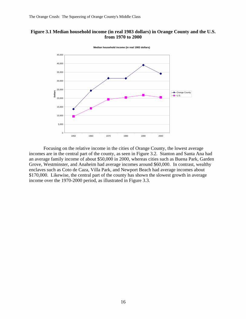
In the last chapter, we saw that those at the lowest level of the income distribution are doing worse in Orange County over the last 30 years. However, how are those at the middle of the income distribution doing? Specifically, consider the median household income in the county: this is the household income at which half of the households have higher income, and half have lower income. To take into account the effects of inflation over this time period, we adjust these values to a constant based on 1983 dollars.2 This graph shows that those at the middle in the income distribution in Orange County are consistently better off than those at the middle of the income distribution in the average U.S. county. Whereas in 1950 the median household income in Orange County was about 40% higher than in an average U.S. county, this jumped to 70% higher by 1960. This relative prosperity continued over the following two decades with the median household income in Orange County exceeding that of an average U.S. county by 50 to 60%. And the 1980’s were a particularly economically dynamic period for the county as the median income shot up to almost 80% higher than the average U.S. county by 1990. However, this advantage diminished during the 1990’s as the county suffered its first decline in real median family income during this particular decade. The real income of the median family declined 12.7% during the 1990’s, and has only increased modestly during the early part of the millenium.

2 We used the consumer price index for these calculations.

15


Figure 3.1 Median household income (in real 1983 dollars) in Orange County and the U.S. from 1970 to 2000

Median household income (in real 1983 dollars)

0

5,000

10,000

15,000

20,000

25,000

30,000

35,000

40,000

45,000

1950 1960 1970 1980 1990 2000

Dol

lars Orange County

U.S.

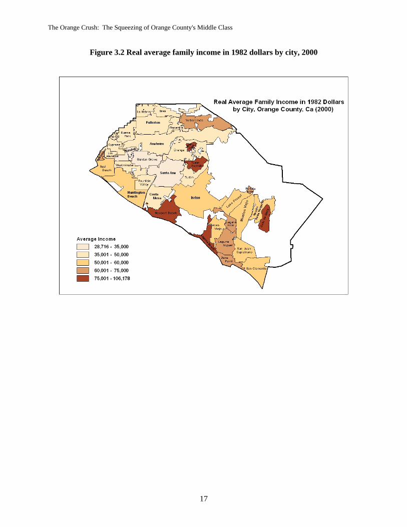
Focusing on the relative income in the cities of Orange County, the lowest average

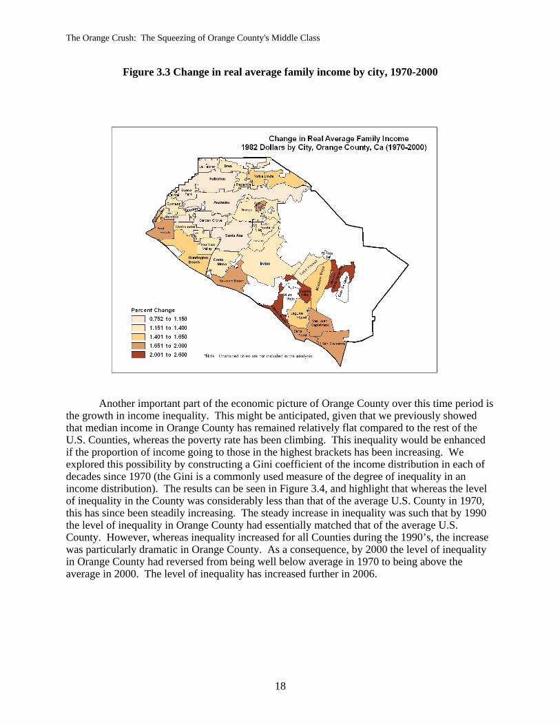
incomes are in the central part of the county, as seen in Figure 3.2. Stanton and Santa Ana had an average family income of about $50,000 in 2000, whereas cities such as Buena Park, Garden Grove, Westminster, and Anaheim had average incomes around $60,000. In contrast, wealthy enclaves such as Coto de Caza, Villa Park, and Newport Beach had average incomes about $170,000. Likewise, the central part of the county has shown the slowest growth in average income over the 1970-2000 period, as illustrated in Figure 3.3.

16


Figure 3.2 Real average family income in 1982 dollars by city, 2000

17


Figure 3.3 Change in real average family income by city, 1970-2000

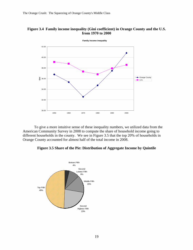
Another important part of the economic picture of Orange County over this time period is

the growth in income inequality. This might be anticipated, given that we previously showed that median income in Orange County has remained relatively flat compared to the rest of the U.S. Counties, whereas the poverty rate has been climbing. This inequality would be enhanced if the proportion of income going to those in the highest brackets has been increasing. We explored this possibility by constructing a Gini coefficient of the income distribution in each of decades since 1970 (the Gini is a commonly used measure of the degree of inequality in an income distribution). The results can be seen in Figure 3.4, and highlight that whereas the level of inequality in the County was considerably less than that of the average U.S. County in 1970, this has since been steadily increasing. The steady increase in inequality was such that by 1990 the level of inequality in Orange County had essentially matched that of the average U.S. County. However, whereas inequality increased for all Counties during the 1990’s, the increase was particularly dramatic in Orange County. As a consequence, by 2000 the level of inequality in Orange County had reversed from being well below average in 1970 to being above the average in 2000. The level of inequality has increased further in 2006.

18


Figure 3.4 Family income inequality (Gini coefficient) in Orange County and the U.S.

from 1970 to 2000

Family income inequality

30.00

32.00

34.00

36.00

38.00

40.00

42.00

1950 1960 1970 1980 1990 2000

Gin

i Orange CountyU.S.

To give a more intuitive sense of these inequality numbers, we utilized data from the American Community Survey in 2008 to compute the share of household income going to different households in the county. We see in Figure 3.5 that the top 20% of households in Orange County accounted for almost half of the total income in 2008.

Figure 3.5 Share of the Pie: Distribution of Aggregate Income by Quintile

Bottom Fifth4%

Second Lowest Fifth

9%

Middle Fifth15%

Second Highest Fifth

23%

Top Fifth49%

19


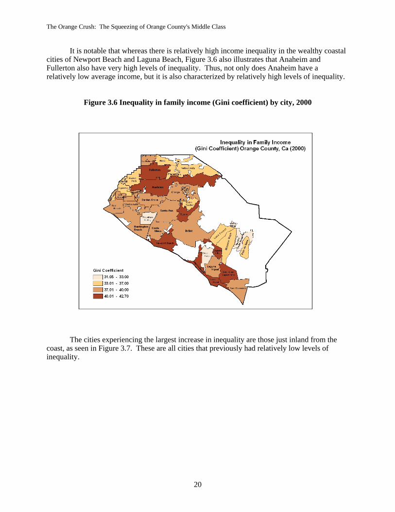
It is notable that whereas there is relatively high income inequality in the wealthy coastal cities of Newport Beach and Laguna Beach, Figure 3.6 also illustrates that Anaheim and Fullerton also have very high levels of inequality. Thus, not only does Anaheim have a relatively low average income, but it is also characterized by relatively high levels of inequality.

Figure 3.6 Inequality in family income (Gini coefficient) by city, 2000

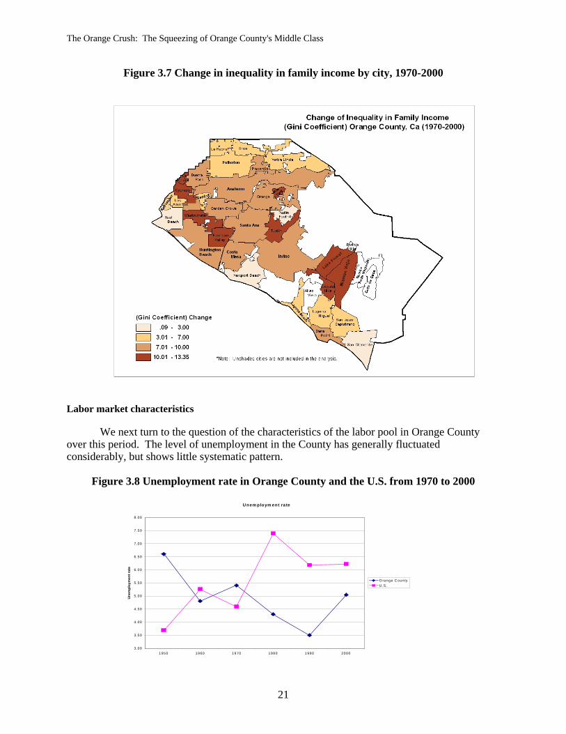
The cities experiencing the largest increase in inequality are those just inland from the

coast, as seen in Figure 3.7. These are all cities that previously had relatively low levels of inequality.

20


Figure 3.7 Change in inequality in family income by city, 1970-2000

Labor market characteristics

We next turn to the question of the characteristics of the labor pool in Orange County over this period. The level of unemployment in the County has generally fluctuated considerably, but shows little systematic pattern.

Figure 3.8 Unemployment rate in Orange County and the U.S. from 1970 to 2000

U nem ploym ent ra te

3 .00

3 .50

4 .00

4 .50

5 .00

5 .50

6 .00

6 .50

7 .00

7 .50

8 .00

1950 1960 1970 1980 1990 2000

Une

mpl

oym

ent r

ate

O range C oun tyU .S .

21


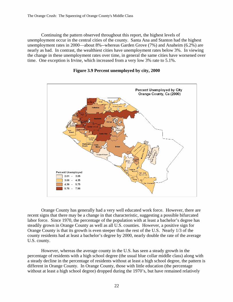
Continuing the pattern observed throughout this report, the highest levels of

unemployment occur in the central cities of the county. Santa Ana and Stanton had the highest unemployment rates in 2000—about 8%--whereas Garden Grove (7%) and Anaheim (6.2%) are nearly as bad. In contrast, the wealthiest cities have unemployment rates below 3%. In viewing the change in these unemployment rates over time, in general the same cities have worsened over time. One exception is Irvine, which increased from a very low 3% rate to 5.1%.

Figure 3.9 Percent unemployed by city, 2000

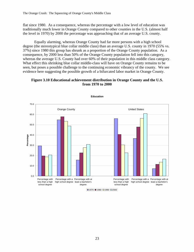
Orange County has generally had a very well educated work force. However, there are recent signs that there may be a change in that characteristic, suggesting a possible bifurcated labor force. Since 1970, the percentage of the population with at least a bachelor’s degree has steadily grown in Orange County as well as all U.S. counties. However, a positive sign for Orange County is that its growth is even steeper than the rest of the U.S. Nearly 1/3 of the county residents had at least a bachelor’s degree by 2000, nearly double the rate of the average U.S. county.

However, whereas the average county in the U.S. has seen a steady growth in the

percentage of residents with a high school degree (the usual blue collar middle class) along with a steady decline in the percentage of residents without at least a high school degree, the pattern is different in Orange County. In Orange County, those with little education (the percentage without at least a high school degree) dropped during the 1970’s, but have remained relatively

22


flat since 1980. As a consequence, whereas the percentage with a low level of education was traditionally much lower in Orange County compared to other counties in the U.S. (almost half the level in 1970) by 2000 the percentage was approaching that of an average U.S. county.

Equally alarming, whereas Orange County had far more persons with a high school

degree (the stereotypical blue collar middle class) than an average U.S. county in 1970 (55% vs. 37%) since 1980 this group has shrunk as a proportion of the Orange County population. As a consequence, by 2000 less than 50% of the Orange County population fell into this category, whereas the average U.S. County had over 60% of their population in this middle class category. What effect this shrinking blue collar middle-class will have on Orange County remains to be seen, but poses a possible challenge to the continuing economic vibrancy of the county. We see evidence here suggesting the possible growth of a bifurcated labor market in Orange County.

Figure 3.10 Educational achievement distribution in Orange County and the U.S. from 1970 to 2000

Education

0.0

10.0

20.0

30.0

40.0

50.0

60.0

70.0

Percentage withless than a highschool degree

Percentage with ahigh school degree

Percentage with atleast a bachelor's

degree

Percentage withless than a highschool degree

Percentage with ahigh school degree

Percentage with atleast a bachelor's

degree

Perc

enta

ge

1970 1980 1990 2000

Orange County United States

23


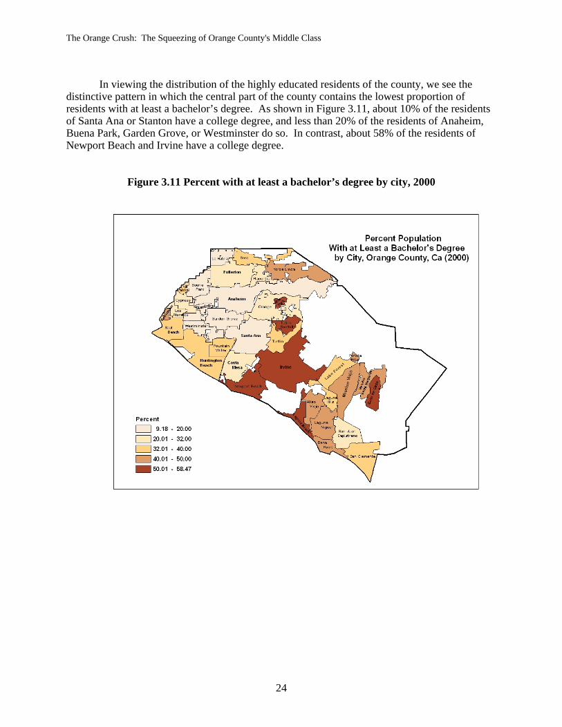
In viewing the distribution of the highly educated residents of the county, we see the

distinctive pattern in which the central part of the county contains the lowest proportion of residents with at least a bachelor’s degree. As shown in Figure 3.11, about 10% of the residents of Santa Ana or Stanton have a college degree, and less than 20% of the residents of Anaheim, Buena Park, Garden Grove, or Westminster do so. In contrast, about 58% of the residents of Newport Beach and Irvine have a college degree.

Figure 3.11 Percent with at least a bachelor’s degree by city, 2000

24


Working Poverty

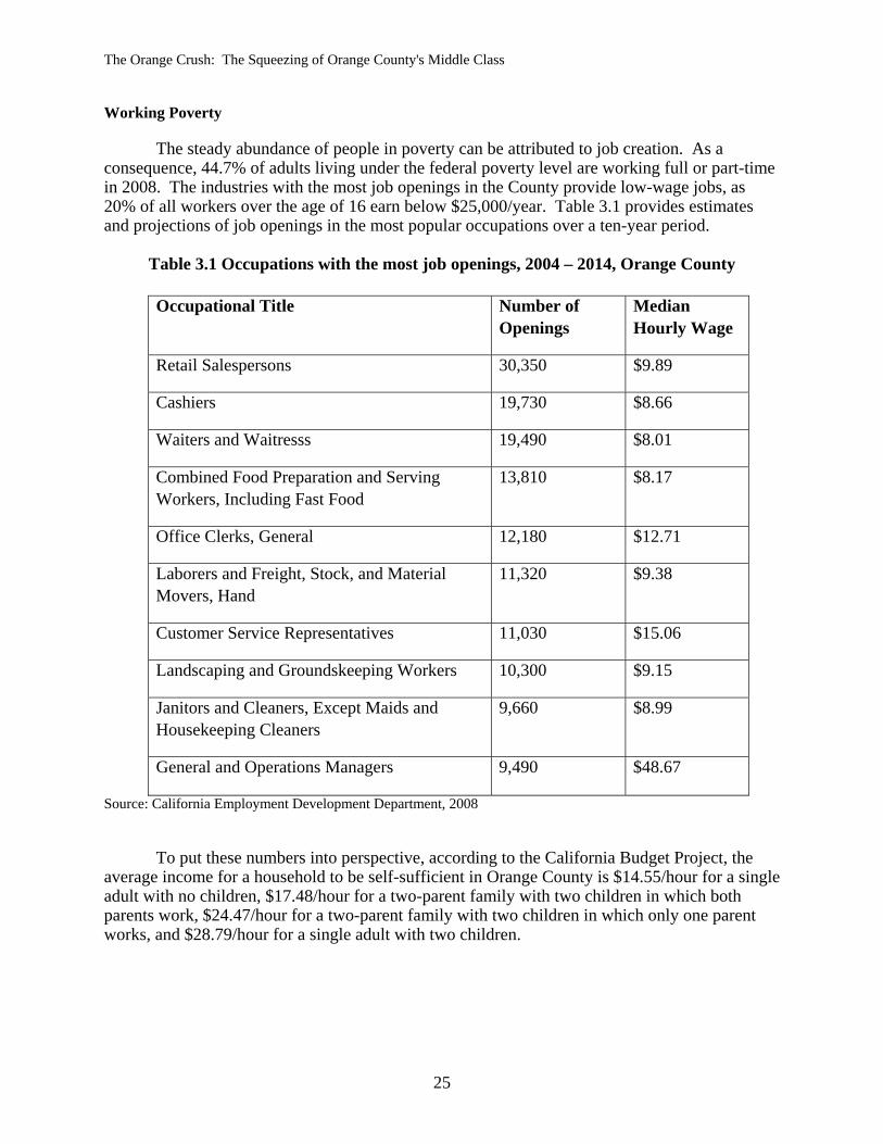
The steady abundance of people in poverty can be attributed to job creation. As a consequence, 44.7% of adults living under the federal poverty level are working full or part-time in 2008. The industries with the most job openings in the County provide low-wage jobs, as 20% of all workers over the age of 16 earn below $25,000/year. Table 3.1 provides estimates and projections of job openings in the most popular occupations over a ten-year period.

Table 3.1 Occupations with the most job openings, 2004 – 2014, Orange County

Occupational Title Number of Openings

Median Hourly Wage

Retail Salespersons 30,350 $9.89

Cashiers 19,730 $8.66

Waiters and Waitresss 19,490 $8.01

Combined Food Preparation and Serving Workers, Including Fast Food

13,810 $8.17

Office Clerks, General 12,180 $12.71

Laborers and Freight, Stock, and Material Movers, Hand

11,320 $9.38

Customer Service Representatives 11,030 $15.06

Landscaping and Groundskeeping Workers 10,300 $9.15

Janitors and Cleaners, Except Maids and Housekeeping Cleaners

9,660 $8.99

General and Operations Managers 9,490 $48.67

Source: California Employment Development Department, 2008

To put these numbers into perspective, according to the California Budget Project, the

average income for a household to be self-sufficient in Orange County is $14.55/hour for a single adult with no children, $17.48/hour for a two-parent family with two children in which both parents work, $24.47/hour for a two-parent family with two children in which only one parent works, and $28.79/hour for a single adult with two children.

25


Chapter 4. Housing and the cost of living In this chapter, we highlight some of the consequences of the growing inequality among

the residents and the workforce in the county that we described in the last chapter. This inequality has been accompanied by an increasing cost of living in the county—based on the ratio of home values and rents to incomes—which results in housing challenges for those at the lower level of the income distribution. While new residents have flocked to the region over the past several decades to soak up the sun and enjoy the beauty of the mountains, ocean, and beautiful year round weather, the cost of living has remained amongst the highest in the nation.

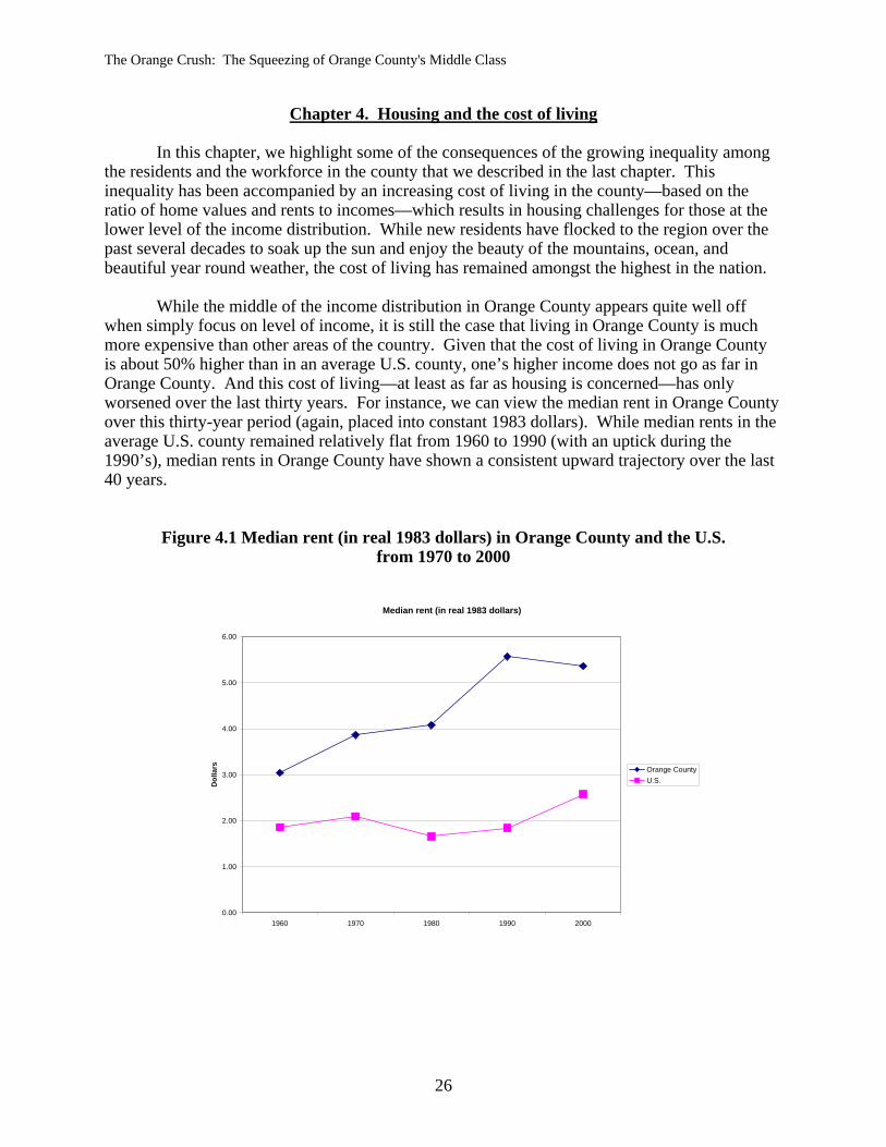
While the middle of the income distribution in Orange County appears quite well off when simply focus on level of income, it is still the case that living in Orange County is much more expensive than other areas of the country. Given that the cost of living in Orange County is about 50% higher than in an average U.S. county, one’s higher income does not go as far in Orange County. And this cost of living—at least as far as housing is concerned—has only worsened over the last thirty years. For instance, we can view the median rent in Orange County over this thirty-year period (again, placed into constant 1983 dollars). While median rents in the average U.S. county remained relatively flat from 1960 to 1990 (with an uptick during the 1990’s), median rents in Orange County have shown a consistent upward trajectory over the last 40 years.

Figure 4.1 Median rent (in real 1983 dollars) in Orange County and the U.S. from 1970 to 2000

Median rent (in real 1983 dollars)

0.00

1.00

2.00

3.00

4.00

5.00

6.00

1960 1970 1980 1990 2000

Dol

lars Orange County

U.S.

26


The hourly wage needed to afford a 2-bedroom apartment in Orange County in 2008 is $30.67/hour (National Low Income Housing Coalition). As noted in the previous chapter, 9 out of the 10 jobs with the most job openings pay significantly less than that. This imbalance has a potential to create overcrowded housing conditions, as families couple together to split rental costs, and several health risks as the propensity for homelessness is increased with such a gap between the cost of living and the jobs provided.

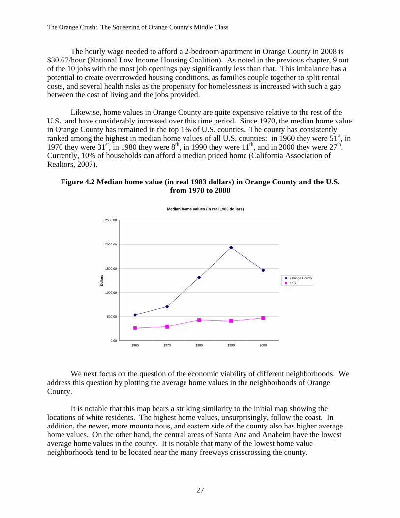
Likewise, home values in Orange County are quite expensive relative to the rest of the

U.S., and have considerably increased over this time period. Since 1970, the median home value in Orange County has remained in the top 1% of U.S. counties. The county has consistently ranked among the highest in median home values of all U.S. counties: in 1960 they were 51st, in 1970 they were 31st, in 1980 they were 8th, in 1990 they were 11th, and in 2000 they were 27th. Currently, 10% of households can afford a median priced home (California Association of Realtors, 2007).

Figure 4.2 Median home value (in real 1983 dollars) in Orange County and the U.S. from 1970 to 2000

Median home values (in real 1983 dollars)

0.00

500.00

1000.00

1500.00

2000.00

2500.00

1960 1970 1980 1990 2000

Dol

lars Orange County

U.S.

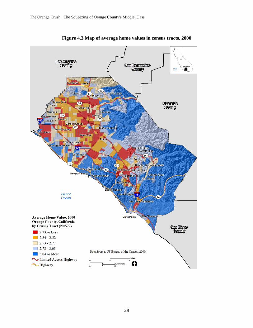
We next focus on the question of the economic viability of different neighborhoods. We address this question by plotting the average home values in the neighborhoods of Orange County.

It is notable that this map bears a striking similarity to the initial map showing the locations of white residents. The highest home values, unsurprisingly, follow the coast. In addition, the newer, more mountainous, and eastern side of the county also has higher average home values. On the other hand, the central areas of Santa Ana and Anaheim have the lowest average home values in the county. It is notable that many of the lowest home value neighborhoods tend to be located near the many freeways crisscrossing the county.

27


Figure 4.3 Map of average home values in census tracts, 2000

28


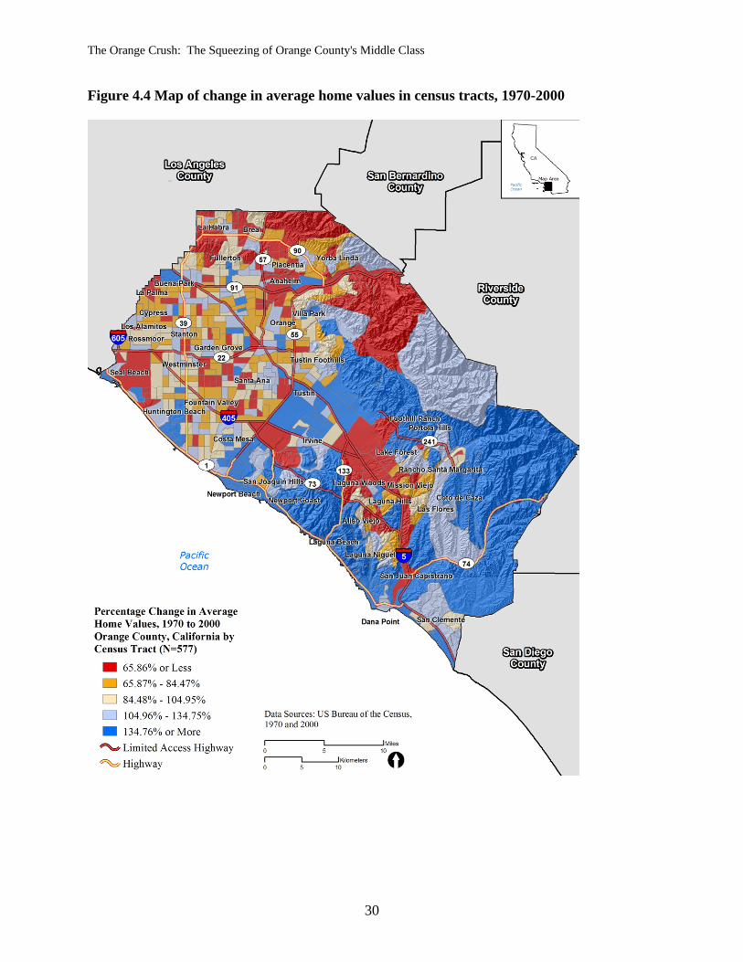
For our final map, we look at the change in average home values in the neighborhoods of Orange County over the 1970 to 2000 period. While there is again evidence that the most southern, and newest, areas have fared the best, the map is not as clearly delineated as the previous ones. We see more evidence here that certain neighborhoods scattered throughout the county have been successful in maintaining their home values. For instance, some of the neighborhoods of Santa Ana have fared quite well, particularly those on the eastern side of the city.

29


Figure 4.4 Map of change in average home values in census tracts, 1970-2000

30


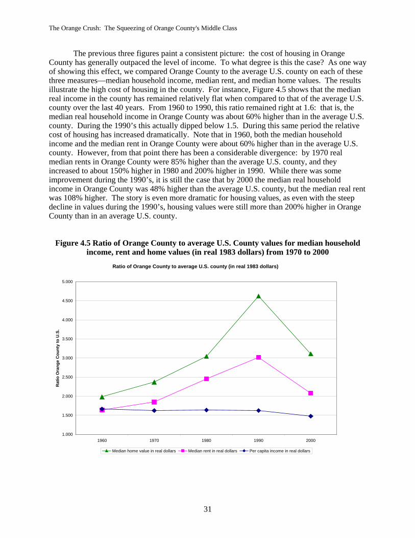
The previous three figures paint a consistent picture: the cost of housing in Orange County has generally outpaced the level of income. To what degree is this the case? As one way of showing this effect, we compared Orange County to the average U.S. county on each of these three measures—median household income, median rent, and median home values. The results illustrate the high cost of housing in the county. For instance, Figure 4.5 shows that the median real income in the county has remained relatively flat when compared to that of the average U.S. county over the last 40 years. From 1960 to 1990, this ratio remained right at 1.6: that is, the median real household income in Orange County was about 60% higher than in the average U.S. county. During the 1990’s this actually dipped below 1.5. During this same period the relative cost of housing has increased dramatically. Note that in 1960, both the median household income and the median rent in Orange County were about 60% higher than in the average U.S. county. However, from that point there has been a considerable divergence: by 1970 real median rents in Orange County were 85% higher than the average U.S. county, and they increased to about 150% higher in 1980 and 200% higher in 1990. While there was some improvement during the 1990’s, it is still the case that by 2000 the median real household income in Orange County was 48% higher than the average U.S. county, but the median real rent was 108% higher. The story is even more dramatic for housing values, as even with the steep decline in values during the 1990’s, housing values were still more than 200% higher in Orange County than in an average U.S. county.

Figure 4.5 Ratio of Orange County to average U.S. County values for median household income, rent and home values (in real 1983 dollars) from 1970 to 2000

Ratio of Orange County to average U.S. county (in real 1983 dollars)

1.000

1.500

2.000

2.500

3.000

3.500

4.000

4.500

5.000

1960 1970 1980 1990 2000

Rat

io O

rang

e C

ount

y to

U.S

.

Median home value in real dollars Median rent in real dollars Per capita income in real dollars

31


Chapter 5. What we have learned, and future directions

This report has documented the dramatic demographic and economic changes in Orange

County, its cities, and its neighborhoods, over the last thirty years. We have documented these large changes, and shown maps of the geographic distribution of various racial/ethnic groups and households of various income levels in the county over time. Our overview of the recent history of Orange County has revealed a broad pattern.

First, the county has shown a huge increase in population along with a considerable

transition in the racial/ethnic composition. The County has transitioned from a largely white population in 1970, to nearly 50% nonwhite in 2000. During the same period immigrants have constituted a constantly growing proportion of the population, and by 2000 represented about 30% of the County’s population. Accompanying this growth in racial/ethnic mixing within cities as a whole is a growth in racial/ethnic segregation of racial/ethnic groups into separate neighborhoods. That is, although the county is becoming more racially/ethnically heterogeneous overall, this heterogeneity does not play out at the neighborhood level. Instead, the neighborhoods of the county tend to exhibit a considerable amount of racial/ethnic homogeneity as a consequence of this segregation.

Second, both income inequality and the cost of living appear to be rising. The percent in

poverty has consistently risen since 1970, and the overall inequality has also risen over that same period. And while the median income has risen, the cost of rent and housing has increased at an even greater rate. One consequence of this is an additional economic burden on the middle and lower class residents of the county. This inequality is accompanied by a growing bifurcation of the workforce based on educational levels. This is a particularly insidious threat to the economic health of the county, as the shrinking proportion of the population with a high school degree is yet a warning indicator of the economic vibrancy of the county. To the extent that the county continues to experience a relatively increasing proportion of those without a high school degree, there may well be an exodus of the type of blue collar jobs that provide a reasonable living wage.

New data reviewed in this report suggests that Orange County’s economic growth is

concentrated in low-wage industries that fail to provide family-supporting wages and benefits. Families of workers in these industries face multiple hurdles to self-sufficiency. On the one hand, wages are insufficient to meet rising housing costs. Orange County is approaching a crisis of housing affordability for working families. On the other hand, many employers in typically low-wage industries fail to provide health insurance for their workers. Low-wage workers and their families must choose to go without health care, pay exorbitant premiums out of their own paychecks, or rely on public programs. The costs to the taxpaying public are significant.

Low quality jobs incur costs for all residents, especially when workers who do not have

access to health insurance rely on publicly-funded health care programs. Because health insurance has become more expensive, Orange County’s children bear an undue burden. In search of cheaper housing, homebuyers have moved further out from job centers. Many employees commute from the Inland Empire, which wreaks havoc on environmental standards for Orange County.

32


Often discussions of development create false choices between uncontrolled growth and no growth at all. I y to implement development policies that generate growth to serve the community we want to build. Other commu

res of new residents every year—and broadening its tax base at the same time.

Angeles and around the nation have helped raise

to

d

nstead, local leaders and residents have an exciting opportunit

nities have faced these same challenges, using local government to mold and shape economic development to deliver better returns for local residents. They focus growth in industries that tend to provide higher-quality jobs and establish minimum development standards that ensure development contributes to raising the quality of life for everyone. Orange County continues to be a destination of lure, attracting sco

Policy implications

Finally, what are some policy implications of these findings? We divide our discussioninto issues that governments are able to address, those that businesses are able to address, and those that the community and labor can address. What government should do:

1. Raise the floor: Government needs to set wage standards that reflect the cost of living. Living wage laws in San Diego, Los the wage floor for tens of thousands of underpaid service workers and should be expanded to cover more employees; Orange County needs to follow suit. The state should follow the lead of ten other states and index the minimum wage to inflation so it reflects increases in the cost of living. Nearly 45% of all individuals in poverty are working.

2. Link public investment to good jobs: Government officials should tie public investment in infrastructure, private development, incentives and other subsidies to the creation ofgood jobs. Those jobs should be made available to communities most in need. Otherwise, taxpayers must pay twice for government subsidies and the cost of low-wage, no benefit employment through expenditures for food stamps, school lunches and public health insurance. Public investment in private development should target industries that are tied to the region and that provide quality jobs or the opportunity to raise job standards.

3. Provide access to quality education: Education levels are highly correlated to economic success, and yet Santa Ana and Anaheim have staggering high school dropout rates. Ofthe 50 states, California ranks 34th in K through 12 education per student spending as ashare of personal income in 2005-06.3 The state should address the fiscal barriersincreasing education spending, and also recognize that addressing poverty is essential to ensuring educational success.

4. Ensure economic security: Our social safety net should enable those who are able to work to participate fully in the economy and enjoy a secure retirement. Children anthose who are unable to work should be protected from economic privation. A functioning social safety net is particularly important during economic downturns, when

3 Jean Ross, “School Finance Facts: How Does California Compare?: Funding California’s Public Schools.” California Budget Project, October 2007.

33


workers lose jobs and see their hours cut.

5. Affordable housing in the area as part of new residential development: The cost of housing in Orange County is exorbitant, ranking among the highest in the nation. Iserved as a major deterrent for attracting young professionals, as well as a burdenseveral working families. Developers must focus more on providing workforce housing close to downtown business centers so that professionals won’t have to seek housing inthe distant regions. Local governments should provide incentives for developerprovide such housing.

t has for

s to

lic services. As Orange County continues to be more densely populated, we

must ensure that we properly fund and protect goods that everyone depends on, such as

ginning to envision life beyond the freeway, as evidenced by the Anaheim Regional Transportation Intermodal Center (ARTIC)

urrently being planned for in Anaheim. This development will link ass-transit lines. Not only does public transit link

What Bu

1. T

y, many business leaders have seen the wisdom of the high road approach, jobs. Business leaders should support

rease

2. Job training opportunities that help workers get better jobs. A coalition of community partners led by the Center on Policy Initiatives in San Diego recently negotiated with

3. A rst source hiring programs provide a structure for

helping local residents take advantage of newly-created jobs, keeping job centers close of

6. Quality pub

fire, police, and libraries. 7. Good public transit. Orange County is be

development that is cit to existing bus services and other mjob centers to housing, but it does so in a way that will be affordable to many.

siness should do:

ake the high road: Orange County’s businesses should recognize that their future is tied to the success of the region, and strive to provide good jobs and decent benefits. Fortunateland are providing good, family-sustaining policies to improve job quality, such as living wage laws and project labor agreements. Such policies make good business sense by allowing firms to compete on the basis of quality and service—rather than by lowering standards—and helping them to incthe productivity of their workforce. Likewise, developers who build mixed-incomehousing are tapping into an important market and ensuring that Orange County’s workforce has a place to live.

JMI/Lennar, the developer of Ball Park Village, to provide job training opportunities to help workers get jobs in the construction of the project and to prepare for the new jobs that would be made available when entertainment, service and retail venues in the development open.4

first-source hiring program. Fi

to housing to alleviate commuting concerns. For instance, as part of the constructionDenver’s new light-rail line, a developer there signed an agreement that, among other things, pledges to hire from the communities adjacent to the development.5

4 Center for Policy Initiatives, www.onlinecpi.org. Retrieved 9/14/08. 5 FRESC, www.fresc.org. Retrieved 9/14/08

34


4. B y employers should provide jobs that meet the housing-wage demands in our market. In 2003, the city of San Jose and a coalition

cery

5. Affordable health insurance. Large corporations should not rely on taxpayer-subsidies to provide health insurance. Medicaid is intended for the truly needy—not for employees

6. Support smart public investment: A healthy business climate requires a well-maintained

infrastructure, a world-class education system and a health care system that works.

of

hat Community and Labor should do:

Develop innovative policy and programs: Labor and community organizations cannot wait for goveneighbor en Jobs Pro s from low ectors.

Organizeworkers The pass workers g janitors, orkers, hotel workers and others have shown that much can be done even in the absence of such legislation.

Transpa e a partnersustainabparticipa The economic direction of Orange County over the next thirty years is in our hands.

etter-paying jobs. Development projects b

of community partners agreed to living wages for parking attendants and future groor hotel workers in a large mixed-use project the city helped build.6 Employers and the greater community benefit with such an arrangement; workers can afford to live near their workplace, thereby providing a steady workforce, and with more income, those workers can buy into employer-based health insurance.

of corporations that can afford to pay their share.

Business leaders should take leadership in supporting smart public investment in schools, public transportation and health care—and should insist that the benefits those programs are broadly shared.

W

rnment leaders to propose policies to address the poverty and inequality that affect their hoods. They need to be at the forefront of crafting new initiatives, such as the Gregram, an initiative of the Los Angeles Apollo Alliance, which aims to prepare resident-income communities for careers in the green manufacturing and green building s

to raise standards: Labor unions have a responsibility to organize unorganized and improve and maintain standards in the industries where workers are represented. age of the Employee Free Choice Act at the federal level should facilitate organizinginto unions by eliminating many of the barriers that now exist. Unions representin security officers, health care w

rency in the development process. We have an opportunity in Orange County to becom in the development process to ensure that growth is in the direction we want to go: le jobs. However, we can only do that if the general public understands and can te in the development process and understand how public resources are being used.

08. 6 www.communitybenefits.org. Retrieved 5/14/

35


References

Dennis J. and Arthur S. Goldberger. 1970. "Estimation of Pareto's Law from Grouped bservations." Journal of the American Statistical Association 65:712-723.

ack P. and Walter T. Martin. 1962. "Urbanization, Technology, and the Division of abor: International Patterns." American Sociological Review 27:667-677.

i, N. C. and N. Podder. 1976. "Efficient Estimation of the

Aigner, O

Gibbs, JL

Kakwan Lorenz Curve and Associated Inequality Measures From Grouped Observations." Econometrica 44:137-148.

NielsI3

Putnam, Robert D. 2000. Bowling Alone: The Collapse and Revival of American Community.

en, Francois and Arthur S. Alderson. 1997. "The Kuznets Curve and the Great U-Turn: ncome Inequality in U.S. Counties, 1970 to 1990." American Sociological Review 62:12-3.

New York: Simon & Schuster.

36


Appendix

ver this

Census

measures.

Americheterogeneity in the city by using a Herfindahl index (Gibbs and Martin 1962: 670) of these

)

where G represents the proportion of the population of ethnic group j out of J ethnic groups. Subtracting from 1 makes this a measure of heterogeneity. We computed economic resources as the median income in the city. We measured overall income inequality by utilizing the Gini coefficient, which is defined as:

(2)

To address the question of how these cities in Orange County have changed o

time period, we utilized data from several sources. Much of the data comes from the U.S. .

We used data from the U.S. decennial censuses to construct our key exogenous

At the city level, we computed the percent of various racial/ethnic groups: white, African-an, Latino, Asian, and other races. We constructed a measure of the racial/ethnic

same five racial/ethnic groupings, which takes the following form:

∑=

−=J

jjGH

1

21 (1

nnix

nG n

i i12

12+

−= ∑ =μ

where xi is the household’s income for 1999 as reported in the 2000 census, μ is the mean income value, the households are arranged in ascending values indexed by i, up to n households in the sample. Because the data are binned (as income is coded into various ranges of values), we will take this into account by utilizing the Pareto-linear procedure (Aigner and Goldberger 1970; Kakwani and Podder 1976), which Nielsen and Alderson (1997) adapted from the U.S. Census Bureau strategy.7

7 We used the prln04.exe program provided by Francois Nielsen at the following website: http://www.unc.edu/~nielsen/data/data.htm.

37

Documents

The Orange Crush: The Squeezing of Orange County's Middle ... · The Orange Crush: The Squeezing of Orange County's Middle Class 1 John R. Hipp* January 28, 2009 ... The Squeezing