SPSShdt2-2012

Research Skills One: Using SPSS 20, Handout 2: Descriptive Statistics: Page 1:

Using SPSS 20: Handout 2. Descriptive statistics: An essential preliminary to any statistical analysis is to obtain some descriptive statistics

for the data obtained - things like means and standard deviations. This handout covers how to obtain these.

The dataset we are going to use is a slightly modified version of one that was supplied as part of the STARS project. It consists of data from a telephone survey investigating people's "fast food" eating habits. 400 people (200 males and 200 females) were asked lots of questions about their personal characteristics (such as their sex, age, and education level) and about their fast food purchasing behaviour (e.g. what brands they bought, how often they did so, and what brand first sprang to mind). The dataset is available on my website.

1. Go to www.sussex.ac.uk/Users/grahamh/RM1web/teaching08-RS.html 2. Click on the link entitled Fast-food study SPSS data. Open the file in SPSS and have a look at it. There are 32 columns (variables) and 400

rows (cases). If you let the cursor hover over a variable name, you will get a longer description of what it's about; most of these are self-explanatory.

Continuous versus categorical variables: There are many things we could investigate using these data. There are also numerous

ways to obtain descriptive statistics in SPSS. One thing that it is very important to keep track of, is whether a variable is continuous (truly numerical) or categorical (or "nominal"). SPSS refers to these as "scale" and "nominal" respectively. If you look at this dataset, you will see that only one of the variables, Purchases, is truly continuous - it consists of the number of fast food purchases in the previous month. It is meaningful to work out averages, etc. on data such as these. All of the other variables in this spreadsheet are categorical measurements - such as whether someone is male or female; whether someone has one kind of education versus another; whether someone first thinks of "MacDonalds" as opposed to "Burger King" or "Starbucks". For variables such as these, all you can do is count how many times each category occurs. You can't calculate the "average" favourite fast food, because there is no way that you can add "MacDonalds" to "Burger King"! With SPSS, you have to be very careful that you are aware of this distinction between continuous and categorical variables, because if you use numbers as labels, SPSS will often happily do statistics on them regardless. For example, in this spreadsheet, "1" is used as a code for "male" and "2" is used for "female". You can ask SPSS to work out the average of the "Sex" variable and it will tell you that it is 1.5 - i.e., the average of 1 and 2, which in this case is obviously nonsense.

To begin with, we will obtain a table of descriptive statistics that will investigate the

continuous variable of Purchases, to answer the following question: do males and females differ in terms of how many times a month they eat fast food?

1. A simple table: how often do men and women eat fast food? Let's produce a table that contains the data on monthly fast food consumption (in the

variable Purchases) broken down by Sex. We'll ask SPSS to show the following descriptive statistics for males and females separately: the mean, median and mode, standard deviation and standard error.

(i) Click on "Analyze" on the SPSS controls at the top of the screen. (ii) Click on "Tables": a small menu will appear to the right. (iii) Click on "Custom Tables...": a dialog box will appear, called "Custom Tables". (Before

this happens, another little warning dialog box may pop up - ignore this and just click "OK" to get rid of it ).

(iv) All of the variables in the dataset are listed in the leftmost box. We put variables that we want to summarise (i.e. ones for which we want statistics) into the right-hand box, by clicking on them and then dragging them near the "columns" graphic (if we want them as a column in our table) or the "rows" graphic (if we want them as rows in the table). Drag the "Purchases" variable


into the box and put it near the "columns" graphic. We want a breakdown of purchases by sex, so drag "Sex" to the "Rows" graphic in the right-hand box. As you do this, SPSS gives you an indication of what the table is going to look like. At the moment, the rows of the table will be "male" and "female", the columns will be the various categories of purchase, and each cell of the table will contain the mean for a particular permutation of sex and purchase.

(v) On the left there is a button labelled "Summary Statistics..." Click on this, and yet

another dialog box appears. (If the "summary statistics" button is greyed out, then click once on the cell of the table labelled "Number of fast food purchases this month" to activate it).

In the left-hand box, click on any statistic that you want performed on your data, so that it

becomes highlighted. Then click on the arrow button between the boxes: the highlighted statistic


should then appear in the right-hand box. You can do this for as many statistics as you like: for this example, highlight "Mean", "Median", "Mode", "Std. Deviation", "S.E. Mean" and "Count". (I always include count, as a check that SPSS is actually calculating the statistics on the same number of cases as I think it is). You will need to use the scroll bar on the right-hand edge of the left box, in order to get to some of the entries.

(vi) Click on "Apply to Selection" once you have highlighted the statistics you want: the dialog box disappears, leaving you with the "Custom Tables" box still open. It now shows you what your output table is going to look like. The dialog box should look like this.

(vii). Click on "OK". The computer will switch to displaying the output window in the

foreground, and you should have a table like the following:

This tells us that, on average, males ate fast food more often than females. For both males and females, the mean, median and mode are all similar, which is an indication that the data are probably normally distributed. The spread of scores (as shown by the s.d.) is a little higher for men than it is for women, suggesting that men are more variable in their fast food eating habits than are women. The s.e.m. is fairly low, suggesting that if we were to repeat the study, we would be likely to get similar results. (On 95% of occasions, the male mean is likely to fall within the range of the mean plus or minus 2 s.e.'s, i.e. within the range of 2.59 to 3.19. For females, on 95% of occasions it is likely to fall somewhere between 1.78 and 2.26). The "count" reassures us that SPSS used 200 males and 200 females in calculating these figures.

Number of fast food purchases last month

Mean Median Mode

Standard

Deviation

Standard Error of

Mean Count

Sex Male 2.89 3.00 3.00 2.07 .15 200

Female 2.02 2.00 2.00 1.76 .12 200


2. A more complex table: fast food consumption, broken down by sex and age: Go through the same process as above. Click on "Analyze", "Tables" and "Custom

Tables", as before, to open the "Custom Tables" dialog box. You don't need to open the "Statistics..." dialog box this time, as SPSS will remember which statistics you want until the end of the session.

This time, put both "sex" and "age" into the rows. Click on "OK", and you should get a table like the following:

You now have the frequency of fast food consumption per month, broken down into each permutation of sex and age. From this table, it appears that for both sexes, the number of purchases decreases with age: on average, the 55-70 year-olds eat fast food half as often as 15-17 year olds.

Try experimenting with various options in the "Custom Tables" box, to see what happens

to the appearance of your table. (Note that SPSS pastes your next analysis output under your existing output. If you don’t

want that, save your output and close the window, so your next analysis will pop up in a new output window. Alternatively, you can delete unwanted output, either by clicking on it directly and then pressing the delete key, or by using the left-hand pane of the output window - highlight the output you want to delete and then press delete).

Number of fast food purchases last month

Mean Median Mode

Standard

Deviation

Standard Error

of Mean Count

Age 15-17 Sex Male 3.32 3.00 3.00 2.12 .42 25

Female 3.50 2.50 1.00 2.81 1.15 6

18-24 Sex Male 4.03 3.00 3.00 1.89 .34 31

Female 2.58 2.00 2.00 1.61 .33 24

25-35 Sex Male 2.61 2.00 3.00 2.02 .32 41

Female 2.42 2.00 2.00 1.72 .22 62

36-54 Sex Male 2.78 2.00 2.00 2.05 .23 80

Female 1.75 1.00 1.00 1.70 .18 88

55-70 Sex Male 1.78 1.00 1.00 1.70 .36 23

Female .85 .00 .00 1.04 .23 20


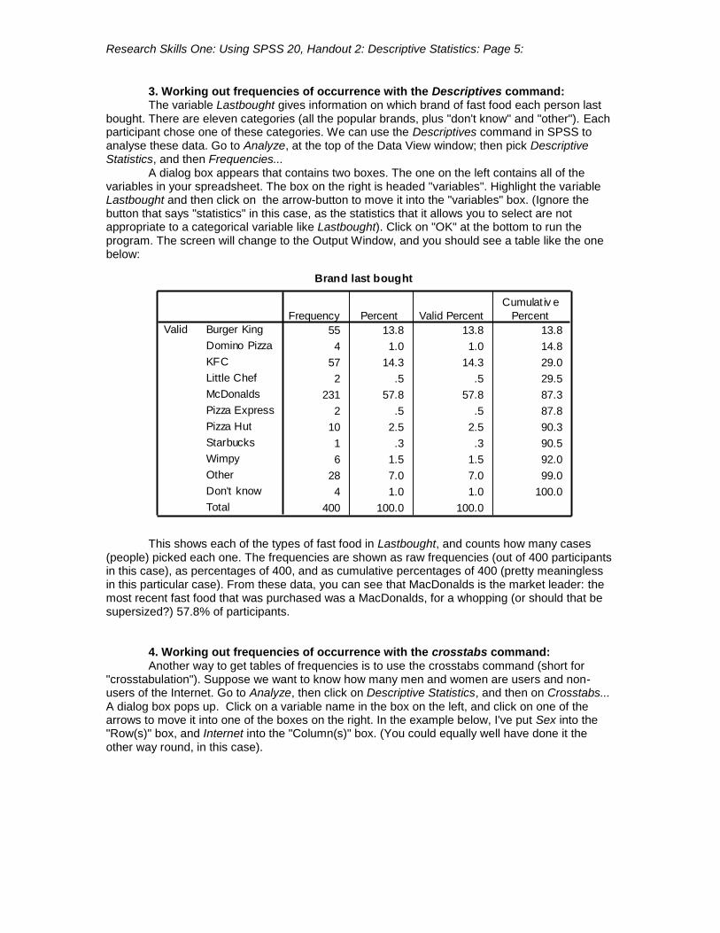
3. Working out frequencies of occurrence with the Descriptives command: The variable Lastbought gives information on which brand of fast food each person last bought. There are eleven categories (all the popular brands, plus "don't know" and "other"). Each participant chose one of these categories. We can use the Descriptives command in SPSS to analyse these data. Go to Analyze, at the top of the Data View window; then pick Descriptive Statistics, and then Frequencies... A dialog box appears that contains two boxes. The one on the left contains all of the variables in your spreadsheet. The box on the right is headed "variables". Highlight the variable Lastbought and then click on the arrow-button to move it into the "variables" box. (Ignore the button that says "statistics" in this case, as the statistics that it allows you to select are not appropriate to a categorical variable like Lastbought). Click on "OK" at the bottom to run the program. The screen will change to the Output Window, and you should see a table like the one below:

Brand last bought

55 13.8 13.8 13.8

4 1.0 1.0 14.8

57 14.3 14.3 29.0

2 .5 .5 29.5

231 57.8 57.8 87.3

2 .5 .5 87.8

10 2.5 2.5 90.3

1 .3 .3 90.5

6 1.5 1.5 92.0

28 7.0 7.0 99.0

4 1.0 1.0 100.0

400 100.0 100.0

Burger King

Domino Pizza

KFC

Little Chef

McDonalds

Pizza Express

Pizza Hut

Starbucks

Wimpy

Other

Don't know

Total

Valid

Frequency Percent Valid Percent

Cumulat iv e

Percent

This shows each of the types of fast food in Lastbought, and counts how many cases

(people) picked each one. The frequencies are shown as raw frequencies (out of 400 participants in this case), as percentages of 400, and as cumulative percentages of 400 (pretty meaningless in this particular case). From these data, you can see that MacDonalds is the market leader: the most recent fast food that was purchased was a MacDonalds, for a whopping (or should that be supersized?) 57.8% of participants.

4. Working out frequencies of occurrence with the crosstabs command: Another way to get tables of frequencies is to use the crosstabs command (short for

"crosstabulation"). Suppose we want to know how many men and women are users and non-users of the Internet. Go to Analyze, then click on Descriptive Statistics, and then on Crosstabs... A dialog box pops up. Click on a variable name in the box on the left, and click on one of the arrows to move it into one of the boxes on the right. In the example below, I've put Sex into the "Row(s)" box, and Internet into the "Column(s)" box. (You could equally well have done it the other way round, in this case).


Click on "OK" and you should get the following table:

Sex * Internet use Crosstabulation

Count

Internet use

Total User Non-user

Sex Male 141 59 200

Female 113 87 200

Total 254 146 400

This shows that 141 males and 113 females use the Internet; 59 males and 87 females

do not. You can produce more complex tables by putting additional variables into the

"Layer" box. For example, this is what you get if you put "Region" into the "Layer" box:

Sex * Internet use * Region lived in Crosstabulation

Count

Region lived in

Internet use

Total User Non-user

Midlands Sex Male 37 18 55

Female 27 22 49

Total 64 40 104

North Sex Male 68 25 93

Female 51 42 93

Total 119 67 186

South Sex Male 36 16 52

Female 35 23 58

Total 71 39 110


Now we have a table that shows us things such as how many Northern women use the Internet; how many Southern males do not use the Internet; and so on.

You can use the "Layer" command to produce even more complex tables! Go back to the Crosstabs dialog box, and now click on the button "Next", near the "Layer" box. The box will show "Layer 2 of 2". Add the variable Listentoradio. Now click "OK", and you will get a table that shows the frequencies of the permutations of radio listening, region, sex and Internet use. I'm going to stop here, as tables this complex make my brain hurt. But if you really wanted to know how many Southern men occasionally listen to the radio but don't use the Internet, then this is the way to find that out.

Sex * Internet use * Region lived in * Listen to radio Crosstabulation

Count

5 2 7

3 4 7

8 6 14

9 3 12

8 11 19

17 14 31

6 4 10

5 7 12

11 11 22

8 7 15

6 6 12

14 13 27

11 12 23

12 13 25

23 25 48

11 5 16

8 6 14

19 11 30

24 9 33

18 12 30

42 21 63

48 10 58

31 18 49

79 28 107

19 7 26

22 10 32

41 17 58

Male

Female

Sex

Total

Male

Female

Sex

Total

Male

Female

Sex

Total

Male

Female

Sex

Total

Male

Female

Sex

Total

Male

Female

Sex

Total

Male

Female

Sex

Total

Male

Female

Sex

Total

Male

Female

Sex

Total

Region liv ed in

Midlands

North

South

Midlands

North

South

Midlands

North

South

Listen to radio

Not at all

Occasionally

Regularly

User Non-user

Internet use

Total

Produce tables to answer the following questions: (1) Are there regional differences in fast food consumption?

(2) How many people live in the Midlands, the North and the South? What percentage of people live in each of these regions?

(3) Does educational background affect fast food consumption? (4) What's the relationship between how often people eat fast food, and how many TV

hours they watched during the week? How does this differ for men and women? (5) Use the crosstabs command to find out how many people fall into the following

category: Midlands males with a secondary school education, who regularly listen to the radio, but only occasionally go to the cinema!


Answers to the questions in Using SPSS 20 Handout 2, Descriptive Statistics: Question 1: Are there regional differences in fast food consumption? Answer is: probably not. All

regions appear to show fairly similar purchasing behaviour.

2.53 2.00 2.00 2.02 .20 104

2.44 2.00 2.00 2.04 .15 186

2.42 2.00 3.00 1.80 .17 110

Number of fast f ood

purchases last month

Midlands



North



South

Region

lived in

Mean Median Mode Std Dev iation

Standard

Error of Mean Count

Question 2: How many people live in the Midlands, the North and the South? What percentage of people live in each of these regions?

Frequency Percent Valid Percent Cumulative

Percent

Valid Midlands 104 26.0 26.0 26.0

North 186 46.5 46.5 72.5

South 110 27.5 27.5 100.0

Total 400 100.0 100.0

Question 3: Does educational background affect fast food consumption? It looks like it does - people

who don't appear to know their educational background (why might this be so?) eat the most junk food. (Mind you, there's only six of them!) There doesn't appear to be much difference between the other groups.

4.83 5.00 7.00 .98 2.40 6

2.08 2.00 3.00 .29 1.85 40

2.15 2.00 .00 .35 1.78 26

2.55 2.00 2.00 .13 1.96 244

2.27 2.00 2.00 .21 1.96 84



don't know



graduate



postgraduate



secondary



technical

college

Educational

background

Mean Median Mode

Standard

Error of Mean Std Dev iation Count

Question 4: What's the relationship between how often people eat fast food, and how many TV hours

they watched during the week? How does this differ for men and women? Looks like more men eat fast food than women, and that to some extent, the more telly they watch, the more often they eat fast food. Bear in mind, though, that these conclusions are based on quite small sample sizes - for example, only two men and two women watched an hour or less TV per week. We need to be very wary of generalisations based on small sample sizes, as they can be quite unreliable. Statistical tests, such as those we'll cover in the spring term, can help us to decide whether observed differences between groups are likely to have occurred by chance or not.


If you are wondering what the group labelled "9" means, this is the code that has been used by the researchers to designate missing data. So there are two men and two women for whom we have no information about telly-watching behaviour.

1.00 1.00 .00 1.00 1.41 2 1.00 1.00 .00 1.00 1.41 2

2.91 3.00 3.00 .50 2.39 23 .93 1.00 1.00 .33 1.28 15

2.94 2.00 1.00 .39 2.25 33 1.69 2.00 .00 .26 1.55 35

2.85 3.00 3.00 .22 1.83 67 2.19 2.00 2.00 .19 1.74 86

2.84 2.50 3.00 .29 2.08 50 2.48 2.00 2.00 .29 1.99 46

3.13 3.00 2.00 .43 2.07 23 1.79 1.00 1.00 .43 1.63 14

3.50 3.50 .00 3.50 4.95 2 1.00 1.00 .00 1.00 1.41 2



Under

1



1 to 2



2 to 3



3 to 5



5 to 10



Over

10



9

TV hours

watched

during

week

Mean Median Mode

Standard


Male

Mean Median Mode

Standard


Female

Sex

Question 5: Use the crosstabs command to find out how many people fall into the following category:

Midlands males with a secondary school education, who regularly listen to the radio, but only occasionally go to the cinema! The answer is 13. Again, note that the number of individuals falling into most of the permutations of variables is very small, limiting the validity of the conclusions we can draw from these data.

Written by Graham Hole, September 2012 - any questions, email

[email protected]


Sex * Educational background * Region lived in * Listen to radio * Go to movies Crosstabulation

Count

0 1 0 1

1 1 1 3

1 2 1 4

1 1 0 2

0 5 1 6

1 6 1 8

1 2 3

0 2 2

1 4 5

1 1 1 3

0 2 0 2

1 3 1 5

1 1 2 1 5

0 0 4 2 6

1 1 6 3 11

1 6 7

0 3 3

1 9 10

0 2 2 4

1 7 0 8

1 9 2 12

1 1 0 6 1 9

0 1 1 5 0 7

1 2 1 11 1 16

1 0 5 0 6

0 1 6 1 8

1 1 11 1 14

1 1 2 1 5

0 1 2 0 3

1 2 4 1 8

1 4 1 6

2 6 3 11

3 10 4 17

2 0 3 0 5

0 1 5 2 8

2 1 8 2 13

7 3 10

9 0 9

16 3 19

0 12 3 15

2 7 5 14

2 19 8 29

3 0 3 2 8

1 1 6 3 11

4 1 9 5 19

2 0 13 10 25

1 1 13 3 18

3 1 26 13 43

0 3 4 26 7 40

1 4 3 19 9 36

1 7 7 45 16 76

0 1 0 7 8 16

1 5 2 9 3 20

1 6 2 16 11 36

0 1 1

1 0 1

1 1 2

1 1 2 0 4

0 0 1 1 2

1 1 3 1 6

1 1 2

2 0 2

3 1 4

1 1 2

1 0 1

2 1 3

0 1 1 1 3

1 1 2 1 5

1 2 3 2 8

1 1

1 1

0 4 0 4

1 0 3 4

1 4 3 8

1 1 6 1 9

0 1 4 1 6

1 2 10 2 15

1 0 3 0 4

0 1 1 2 4

1 1 4 2 8

Male

Female

Sex

Total

Male

Female

Sex

Total

Male

Female

Sex

Total

Male

Female

Sex

Total

Male

Female

Sex

Total

Male

Female

Sex

Total

Male

Female

Sex

Total

Male

Female

Sex

Total

Male

Female

Sex

Total

Male

Female

Sex

Total

Male

Female

Sex

Total

Male

Female

Sex

Total

Male

Female

Sex

Total

Male

Female

Sex

Total

Male

Female

Sex

Total

Male

Female

Sex

Total

Male

Female

Sex

Total

Male

Female

Sex

Total

Male

Female

Sex

Total

Male

Female

Sex

Total

Male

Female

Sex

Total

Male

Female

Sex

Total

Male

Female

Sex

Total

MaleSex

Total

Male

Female

Sex

Total

Male

Female

Sex

Total

Male

Female

Sex

Total

Region liv ed in

Midlands

North

South

Midlands

North

South

Midlands

North

South

Midlands

North

South

Midlands

North

South

Midlands

North

South

Midlands

North

South

Midlands

North

South

Midlands

North

South

Listen to radio

Not at all

Occasionally

Regularly

Not at all

Occasionally

Regularly

Not at all

Occasionally

Regularly

Go to mov ies

Not at all

Occasionally

Regularly

don't know graduate postgraduate secondary

technical

college

Educational background

Total

Documents

SPSShdt2-2012