Embed Size (px)
Citation preview
The Two Sample t
Review significance testingReview t distribution
Introduce 2 Sample t test / SPSS
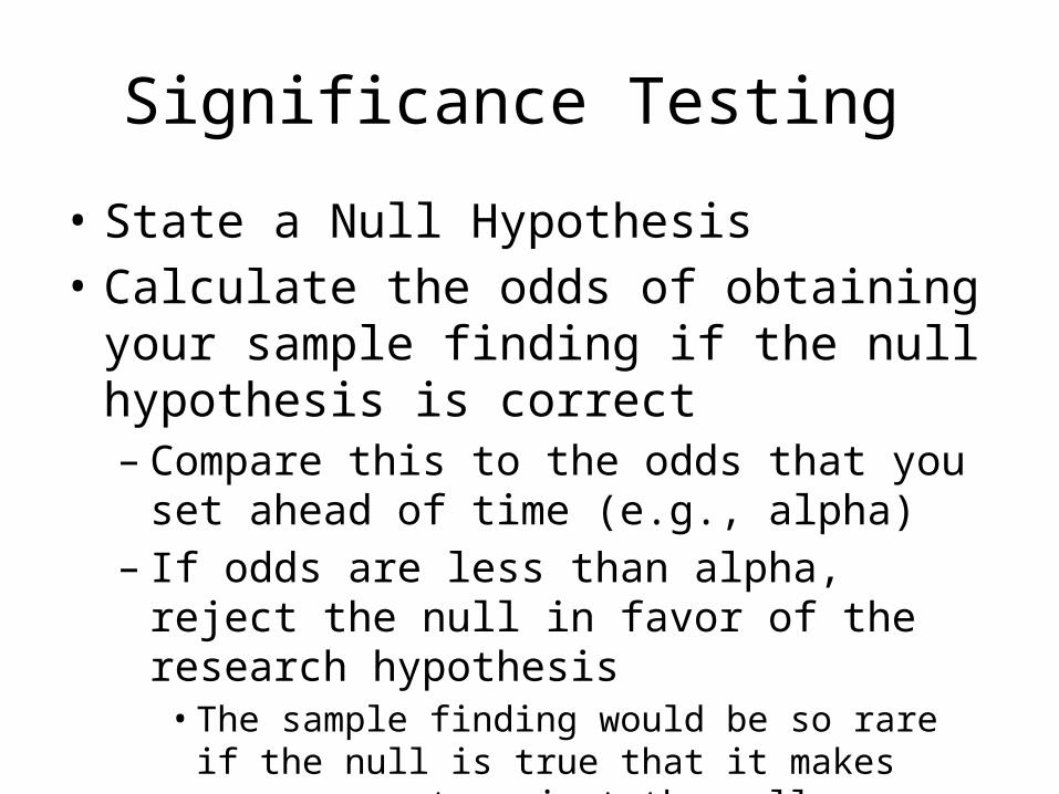
Significance Testing
• State a Null Hypothesis • Calculate the odds of obtaining your sample
finding if the null hypothesis is correct – Compare this to the odds that you set ahead of
time (e.g., alpha)– If odds are less than alpha, reject the null in favor
of the research hypothesis• The sample finding would be so rare if the null is true
that it makes more sense to reject the null hypothesis
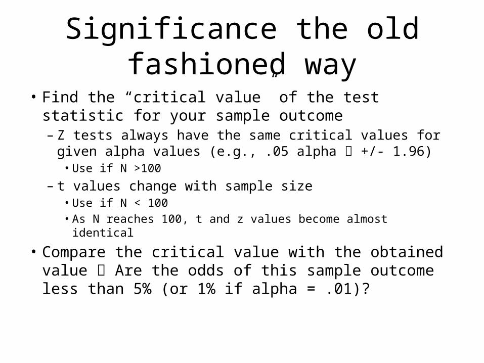
Significance the old fashioned way
• Find the “critical value” of the test statistic for your sample outcome– Z tests always have the same critical values for given alpha
values (e.g., .05 alpha +/- 1.96)• Use if N >100
– t values change with sample size • Use if N < 100• As N reaches 100, t and z values become almost identical
• Compare the critical value with the obtained value Are the odds of this sample outcome less than 5% (or 1% if alpha = .01)?
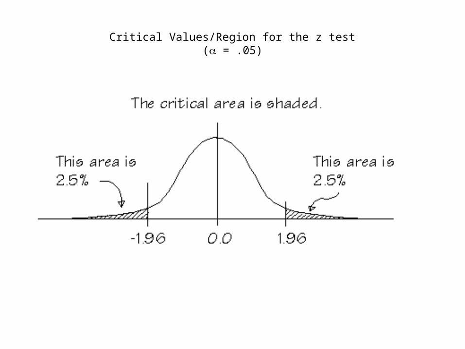
Critical Values/Region for the z test( = .05)
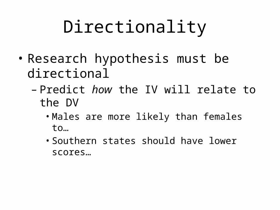
Directionality
• Research hypothesis must be directional – Predict how the IV will relate to the DV
• Males are more likely than females to…• Southern states should have lower scores…
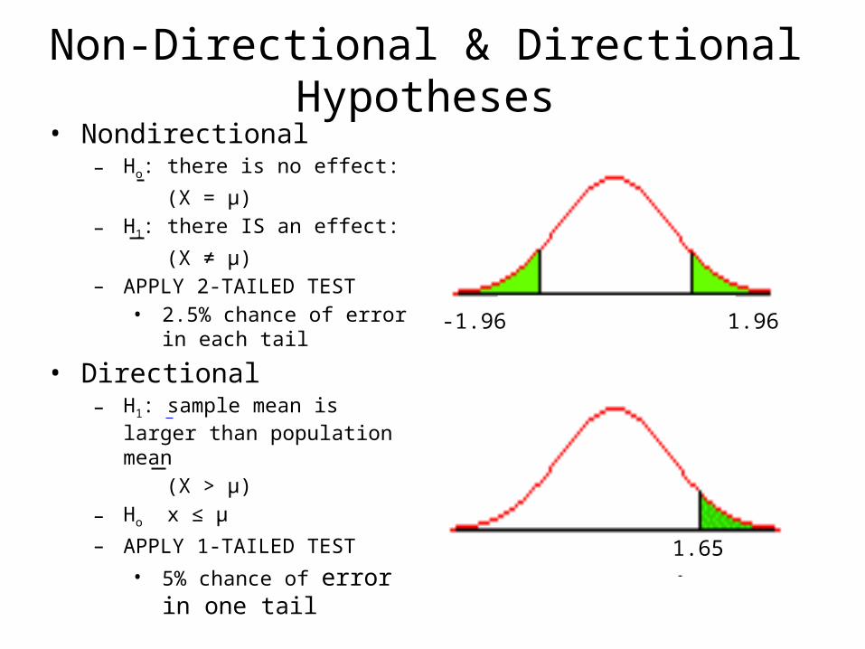
Non-Directional & Directional Hypotheses• Nondirectional
– Ho: there is no effect:
(X = µ)– H1: there IS an effect:
(X ≠ µ)– APPLY 2-TAILED TEST
• 2.5% chance of error in each tail
• Directional– H1: sample mean is larger than
population mean (X > µ)– Ho x ≤ µ– APPLY 1-TAILED TEST
• 5% chance of error in one tail
-1.96 1.96
1.65
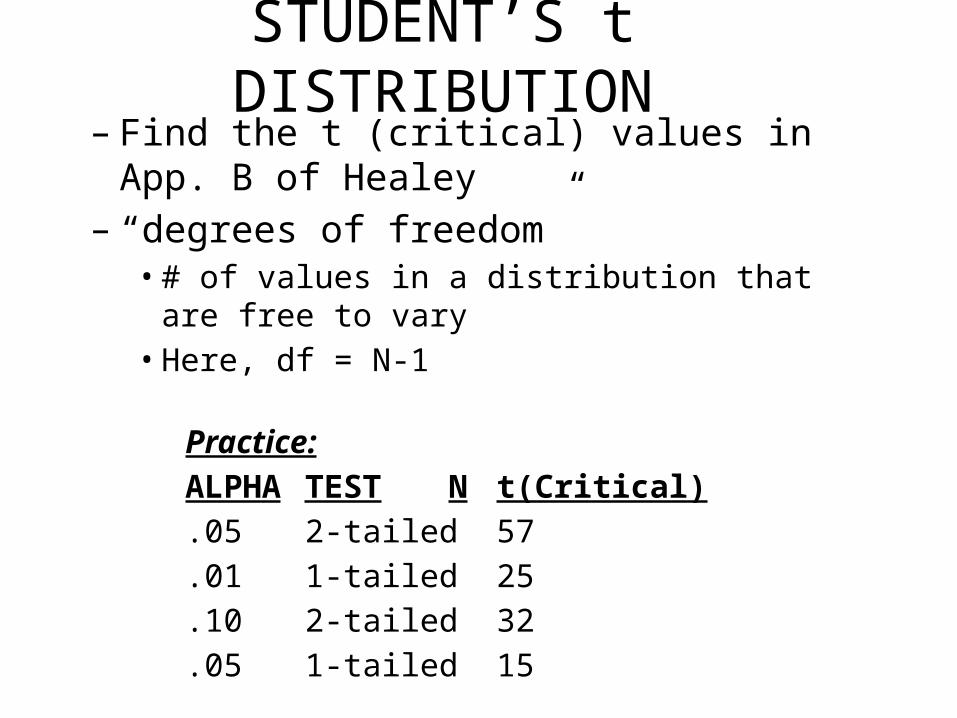
STUDENT’S t DISTRIBUTION– Find the t (critical) values in App. B of Healey– “degrees of freedom”
• # of values in a distribution that are free to vary• Here, df = N-1
Practice:ALPHA TEST N t(Critical).05 2-tailed 57.01 1-tailed 25.10 2-tailed 32.05 1-tailed 15
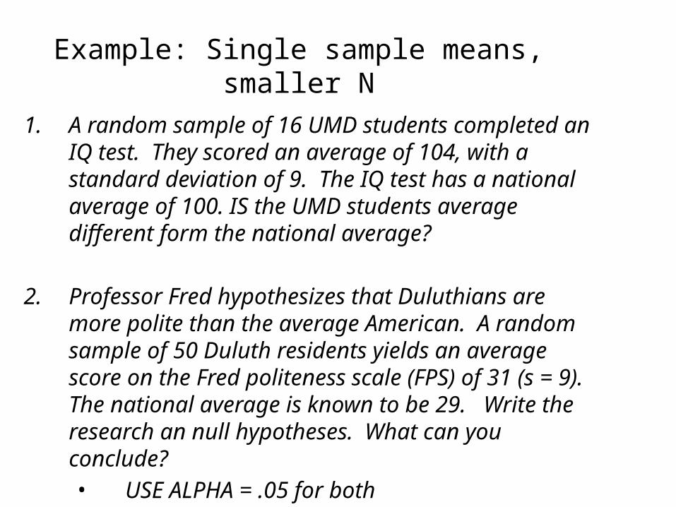
Example: Single sample means, smaller N
1. A random sample of 16 UMD students completed an IQ test. They scored an average of 104, with a standard deviation of 9. The IQ test has a national average of 100. IS the UMD students average different form the national average?
2. Professor Fred hypothesizes that Duluthians are more polite than the average American. A random sample of 50 Duluth residents yields an average score on the Fred politeness scale (FPS) of 31 (s = 9). The national average is known to be 29. Write the research an null hypotheses. What can you conclude?• USE ALPHA = .05 for both
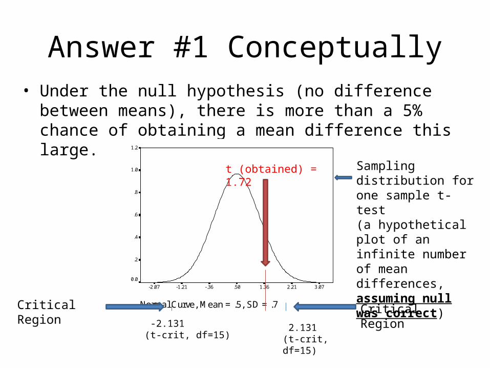
Answer #1 Conceptually• Under the null hypothesis (no difference between means),
there is more than a 5% chance of obtaining a mean difference this large.
Normal Curve, Mean = .5, SD = .7
3.072.211.36.50-.36-1.21-2.07
1.2
1.0
.8
.6
.4
.2
0.0
-2.131(t-crit, df=15)
Sampling distribution for one sample t-test(a hypothetical plot of an infinite number of mean differences, assuming null was correct)
2.131(t-crit, df=15)
Critical Region
t (obtained) = 1.72
Critical Region
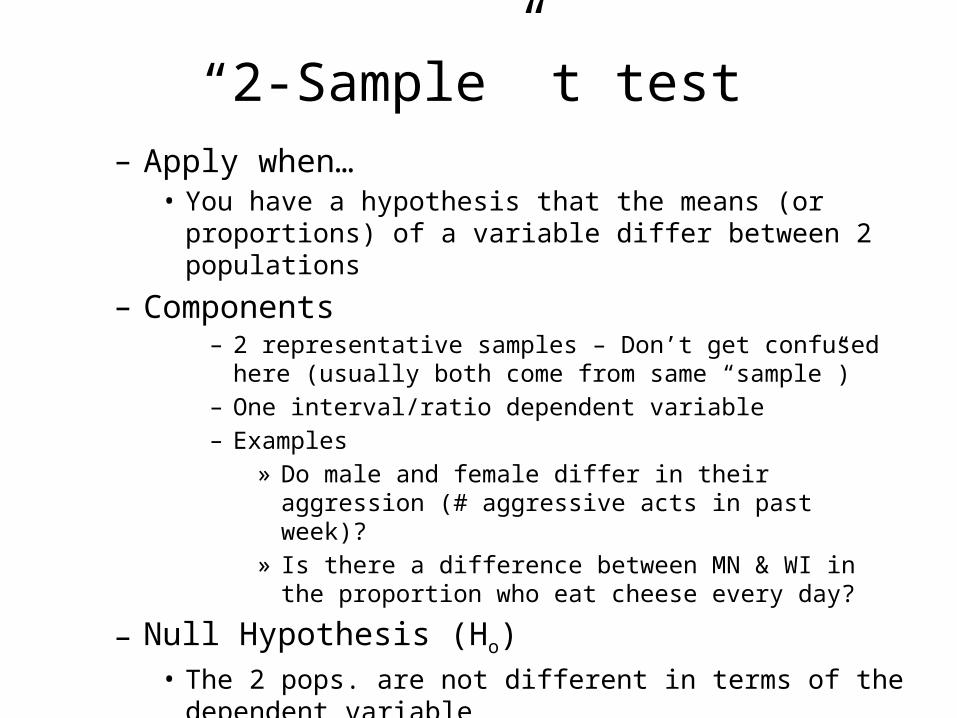
“2-Sample” t test – Apply when…
• You have a hypothesis that the means (or proportions) of a variable differ between 2 populations
– Components– 2 representative samples – Don’t get confused here (usually both
come from same “sample”)– One interval/ratio dependent variable– Examples
» Do male and female differ in their aggression (# aggressive acts in past week)?
» Is there a difference between MN & WI in the proportion who eat cheese every day?
– Null Hypothesis (Ho)• The 2 pops. are not different in terms of the dependent variable
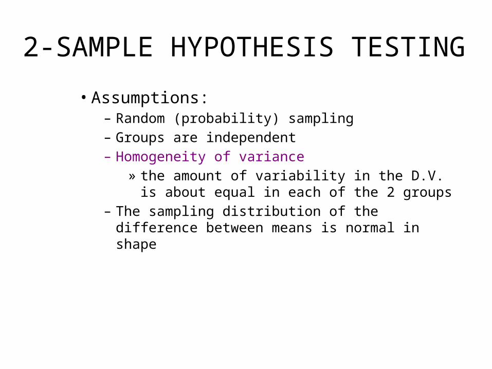
2-SAMPLE HYPOTHESIS TESTING
• Assumptions:– Random (probability) sampling– Groups are independent– Homogeneity of variance
» the amount of variability in the D.V. is about equal in each of the 2 groups
– The sampling distribution of the difference between means is normal in shape
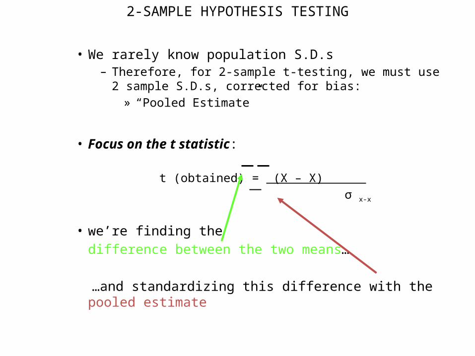
2-SAMPLE HYPOTHESIS TESTING
• We rarely know population S.D.s– Therefore, for 2-sample t-testing, we must use 2 sample S.D.s,
corrected for bias:» “Pooled Estimate”
• Focus on the t statistic:
t (obtained) = (X – X) σ x-x
• we’re finding the difference between the two means…
…and standardizing this difference with the pooled estimate
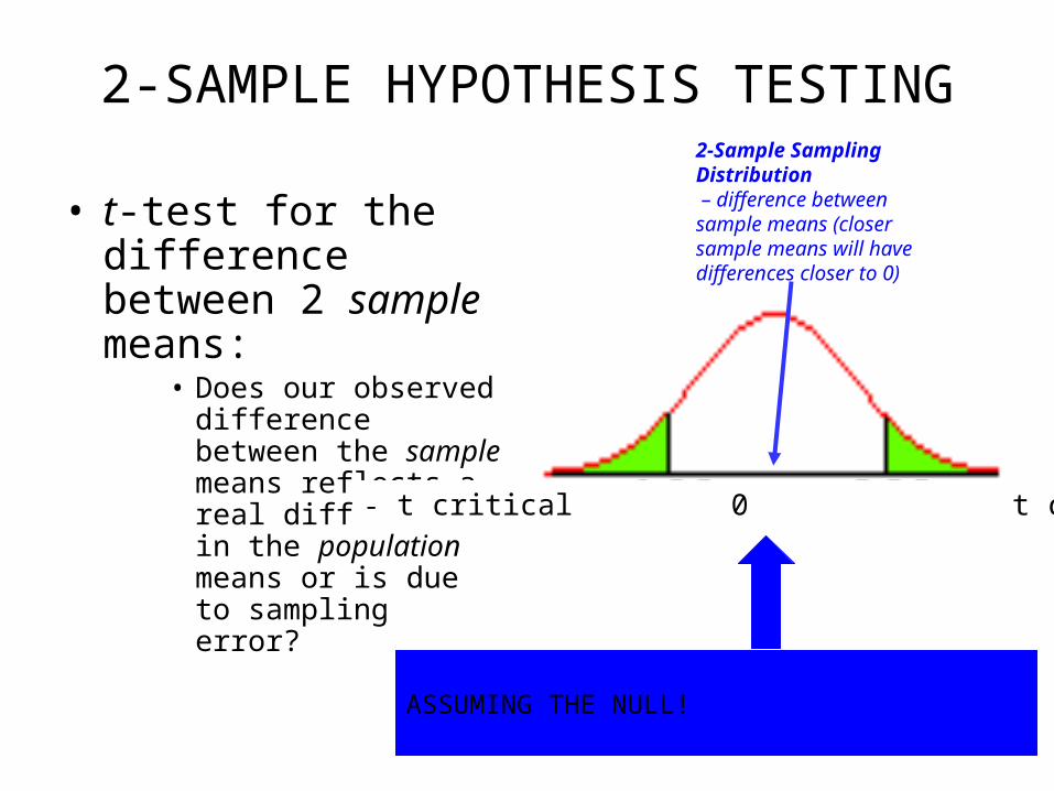
2-SAMPLE HYPOTHESIS TESTING
• t-test for the difference between 2 sample means:
• Does our observed difference between the sample means reflects a real difference in the population means or is due to sampling error? - t critical 0 t critical
2-Sample Sampling Distribution – difference between sample means (closer sample means will have differences closer to 0)
ASSUMING THE NULL!
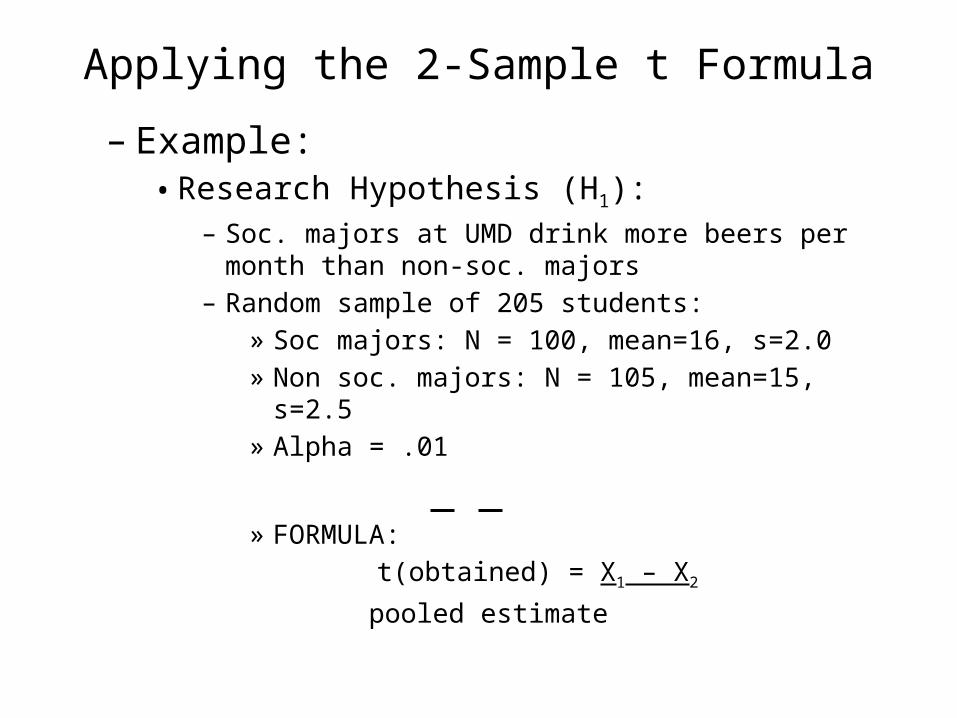
Applying the 2-Sample t Formula
– Example:• Research Hypothesis (H1):
– Soc. majors at UMD drink more beers per month than non-soc. majors
– Random sample of 205 students:» Soc majors: N = 100, mean=16, s=2.0» Non soc. majors: N = 105, mean=15, s=2.5» Alpha = .01
» FORMULA: t(obtained) = X1 – X2
pooled estimate
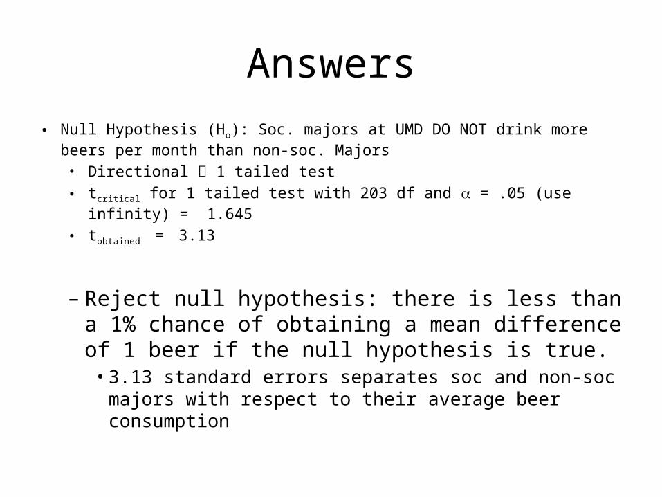
Answers• Null Hypothesis (Ho): Soc. majors at UMD DO NOT drink more beers per
month than non-soc. Majors• Directional 1 tailed test• tcritical for 1 tailed test with 203 df and = .05 (use infinity) = 1.645
• tobtained = 3.13
– Reject null hypothesis: there is less than a 1% chance of obtaining a mean difference of 1 beer if the null hypothesis is true.
• 3.13 standard errors separates soc and non-soc majors with respect to their average beer consumption
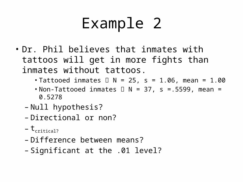
Example 2
• Dr. Phil believes that inmates with tattoos will get in more fights than inmates without tattoos.
• Tattooed inmates N = 25, s = 1.06, mean = 1.00• Non-Tattooed inmates N = 37, s =.5599, mean = 0.5278
– Null hypothesis? – Directional or non?– tcritical? – Difference between means? – Significant at the .01 level?
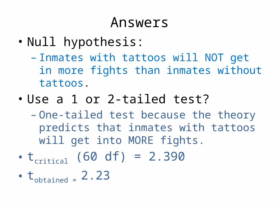
Answers• Null hypothesis:
– Inmates with tattoos will NOT get in more fights than inmates without tattoos.
• Use a 1 or 2-tailed test? – One-tailed test because the theory predicts that
inmates with tattoos will get into MORE fights.
• tcritical (60 df) = 2.390
• tobtained = 2.23
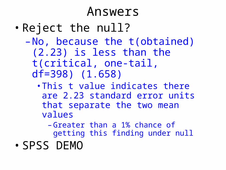
Answers• Reject the null?
– No, because the t(obtained) (2.23) is less than the t(critical, one-tail, df=398) (1.658)• This t value indicates there are 2.23
standard error units that separate the two mean values
– Greater than a 1% chance of getting this finding under null
• SPSS DEMO
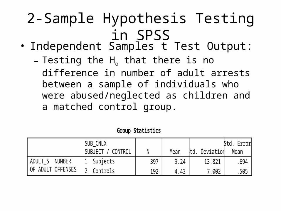
2-Sample Hypothesis Testing in SPSS• Independent Samples t Test Output:
– Testing the Ho that there is no difference in number of adult arrests between a sample of individuals who were abused/neglected as children and a matched control group.
Group Statistics
397 9.24 13.821 .694
192 4.43 7.002 .505
SUB_CNLX SUBJECT / CONTROL1 Subjects
2 Controls
ADULT_S NUMBEROF ADULT OFFENSES
N Mean Std. DeviationStd. Error
Mean
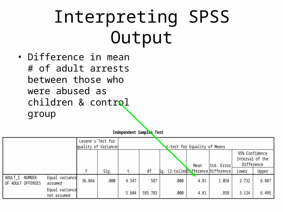
Interpreting SPSS Output
• Difference in mean # of adult arrests between those who were abused as children & control group
Independent Samples Test
36.864 .000 4.547 587 .000 4.81 1.058 2.732 6.887
5.604 585.783 .000 4.81 .858 3.124 6.495
Equal variancesassumed
Equal variancesnot assumed
ADULT_S NUMBEROF ADULT OFFENSES
F Sig.
Levene's Test forEquality of Variances
t df Sig. (2-tailed)Mean
DifferenceStd. ErrorDifference Lower Upper
95% ConfidenceInterval of the
Difference
t-test for Equality of Means
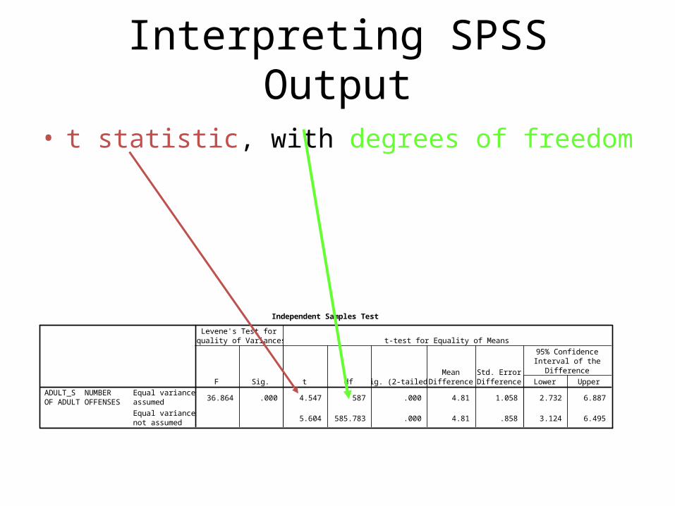
Interpreting SPSS Output
• t statistic, with degrees of freedom
Independent Samples Test
36.864 .000 4.547 587 .000 4.81 1.058 2.732 6.887
5.604 585.783 .000 4.81 .858 3.124 6.495
Equal variancesassumed
Equal variancesnot assumed
ADULT_S NUMBEROF ADULT OFFENSES
F Sig.
Levene's Test forEquality of Variances
t df Sig. (2-tailed)Mean
DifferenceStd. ErrorDifference Lower Upper
95% ConfidenceInterval of the
Difference
t-test for Equality of Means
Interpreting SPSS Output
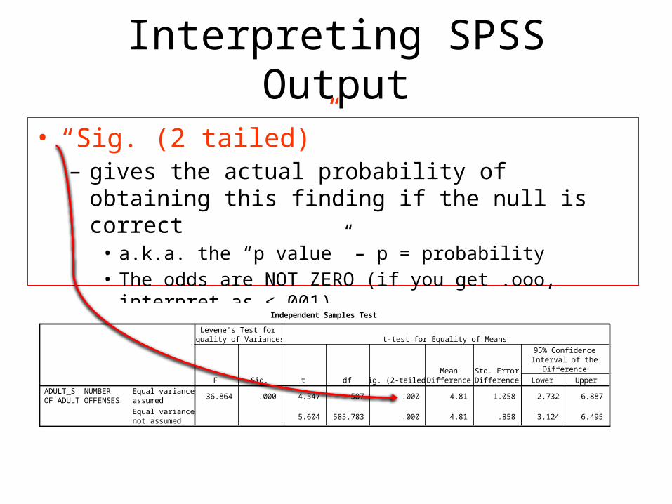
• “Sig. (2 tailed)”– gives the actual probability of obtaining this finding if the
null is correct• a.k.a. the “p value” – p = probability• The odds are NOT ZERO (if you get .ooo, interpret as <.001)
Independent Samples Test
36.864 .000 4.547 587 .000 4.81 1.058 2.732 6.887
5.604 585.783 .000 4.81 .858 3.124 6.495
Equal variancesassumed
Equal variancesnot assumed
ADULT_S NUMBEROF ADULT OFFENSES
F Sig.
Levene's Test forEquality of Variances
t df Sig. (2-tailed)Mean
DifferenceStd. ErrorDifference Lower Upper
95% ConfidenceInterval of the
Difference
t-test for Equality of Means
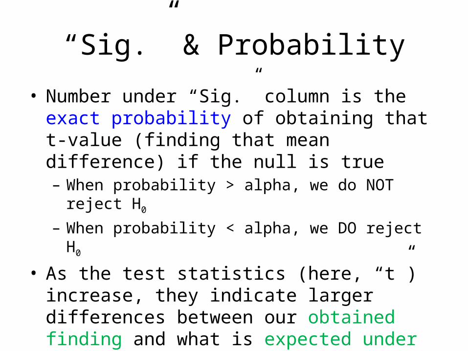
“Sig.” & Probability
• Number under “Sig.” column is the exact probability of obtaining that t-value (finding that mean difference) if the null is true– When probability > alpha, we do NOT reject H0
– When probability < alpha, we DO reject H0
• As the test statistics (here, “t”) increase, they indicate larger differences between our obtained finding and what is expected under null– Therefore, as the test statistic increases, the probability
associated with it decreases
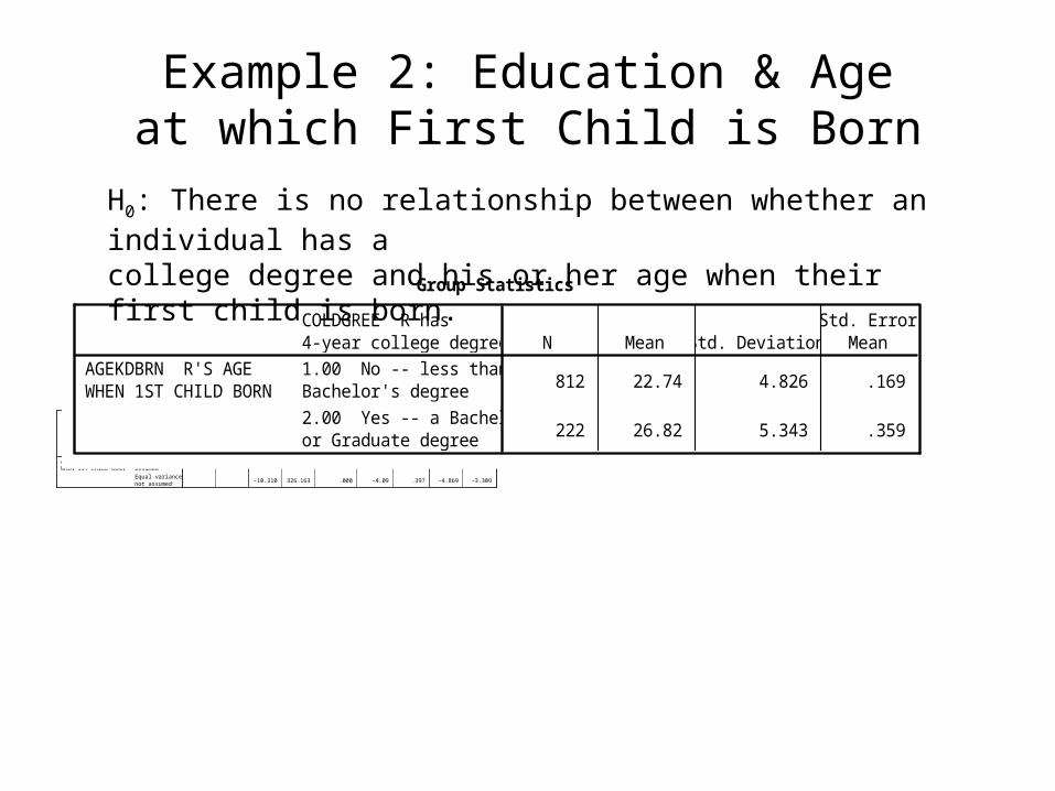
Example 2: Education & Ageat which First Child is Born
Independent Samples Test
4.547 .033 -10.926 1032 .000 -4.09 .374 -4.824 -3.355
-10.310 326.163 .000 -4.09 .397 -4.869 -3.309
Equal variancesassumed
Equal variancesnot assumed
AGEKDBRN R'S AGEWHEN 1ST CHILD BORN
F Sig.
Levene's Test forEquality of Variances
t df Sig. (2-tailed)Mean
DifferenceStd. ErrorDifference Lower Upper
95% ConfidenceInterval of the
Difference
t-test for Equality of Means
Group Statistics
812 22.74 4.826 .169
222 26.82 5.343 .359
COLDGREE R has4-year college degree1.00 No -- less than aBachelor's degree
2.00 Yes -- a Bachelor'sor Graduate degree
AGEKDBRN R'S AGEWHEN 1ST CHILD BORN
N Mean Std. DeviationStd. Error
Mean
H0: There is no relationship between whether an individual has a college degree and his or her age when their first child is born.
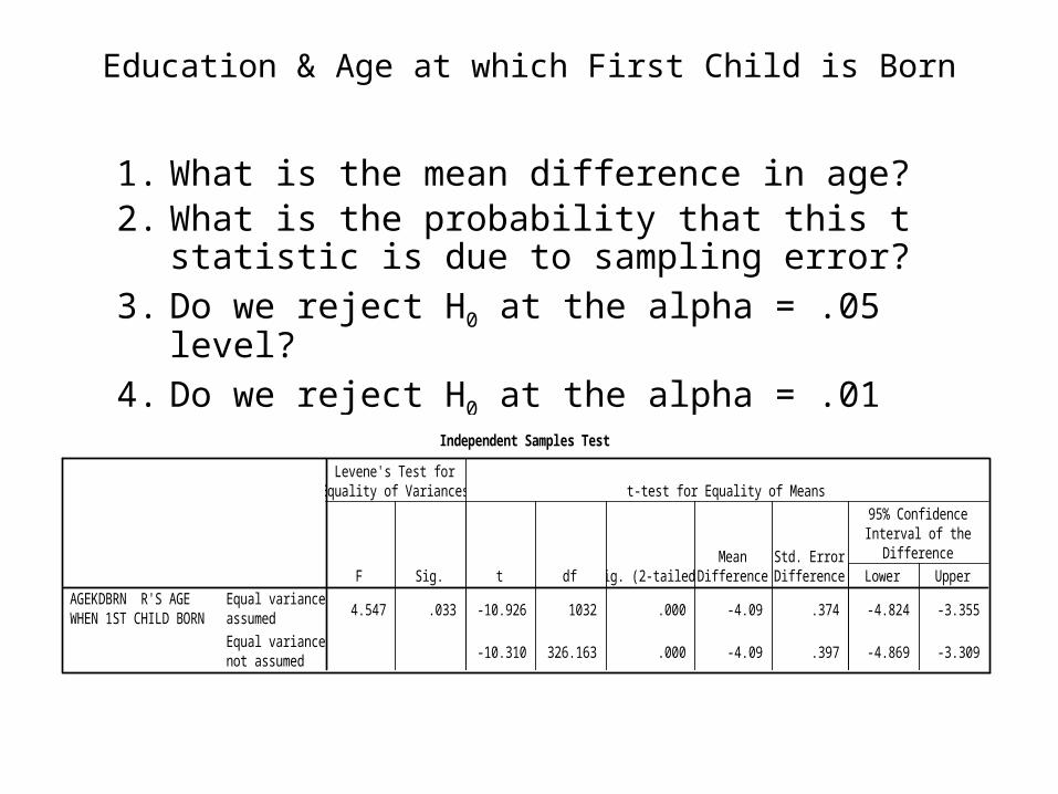
Education & Age at which First Child is Born
1. What is the mean difference in age?2. What is the probability that this t statistic is due to
sampling error?3. Do we reject H0 at the alpha = .05 level?4. Do we reject H0 at the alpha = .01 level?
Independent Samples Test
4.547 .033 -10.926 1032 .000 -4.09 .374 -4.824 -3.355
-10.310 326.163 .000 -4.09 .397 -4.869 -3.309
Equal variancesassumed
Equal variancesnot assumed
AGEKDBRN R'S AGEWHEN 1ST CHILD BORN
F Sig.
Levene's Test forEquality of Variances
t df Sig. (2-tailed)Mean
DifferenceStd. ErrorDifference Lower Upper
95% ConfidenceInterval of the
Difference
t-test for Equality of Means