Crash Modification Factors & Functions

Spring 2013

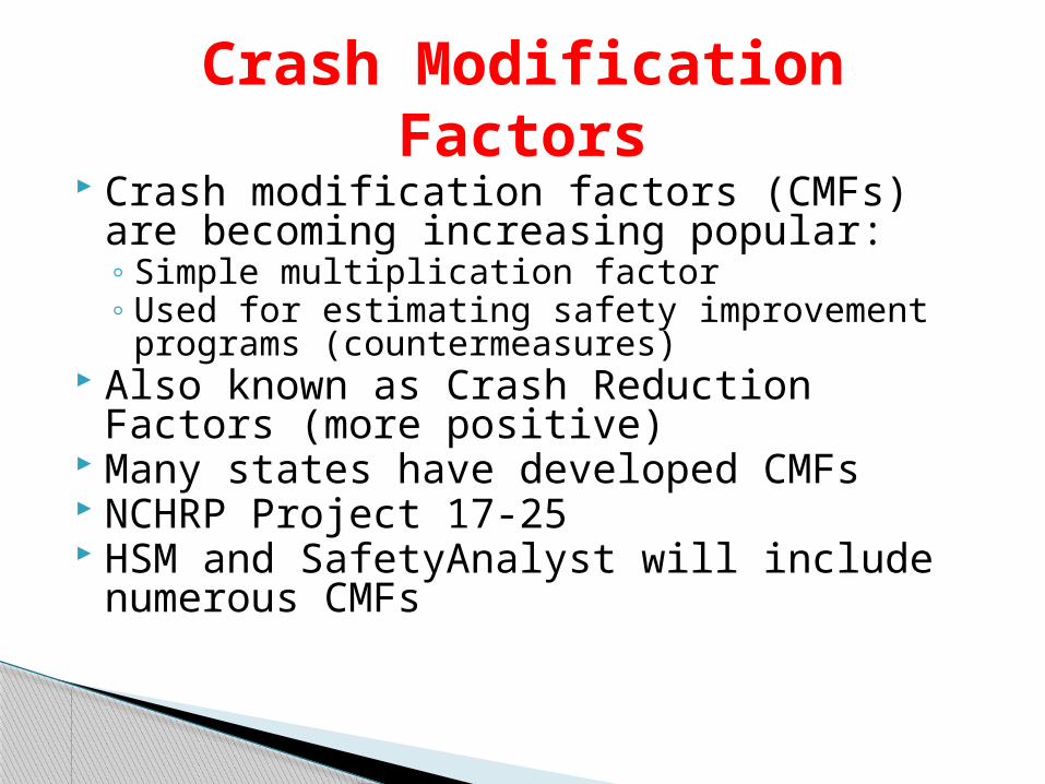
Crash modification factors (CMFs) are becoming increasing popular:◦ Simple multiplication factor◦ Used for estimating safety improvement

programs (countermeasures) Also known as Crash Reduction Factors

(more positive) Many states have developed CMFs NCHRP Project 17-25 HSM and SafetyAnalyst will include

numerous CMFs

Crash Modification Factors

http://www.cmfclearinghouse.org/

http://safety.fhwa.dot.gov/tools/crf/resources/fhwasa10032/

Crash Modification Factors

History about CMFs

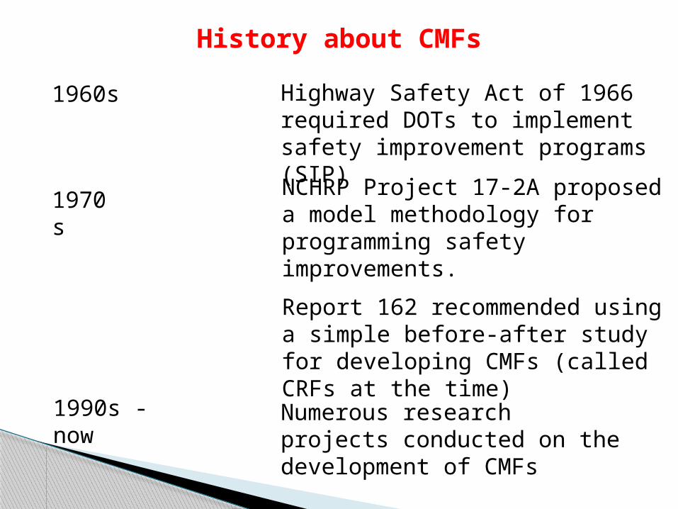
1960s

1970s

1990s - now

Highway Safety Act of 1966 required DOTs to implement safety improvement programs (SIP)NCHRP Project 17-2A proposed a model methodology for programming safety improvements.

Report 162 recommended using a simple before-after study for developing CMFs (called CRFs at the time)Numerous research projects conducted on the development of CMFs

General Framework

A CMF is a multiplicative factor used to compute the expected number of crashes after implementing a given countermeasure at a specific site. The CMF is multiplied by the expected crash frequency without treatment. A CMF greater than 1.0 indicates an expected increase in crashes, while a value less than 1.0 indicates an expected reduction in crashes after implementation of a given countermeasure. For example, a CMF of 0.8 indicates an expected safety benefit; specifically, a 20 percent expected reduction in crashes. A CMF of 1.2 indicates an expected degradation in safety; specifically, a 20 percent expected increase in crashes.

Crash Modification Factor

General Framework

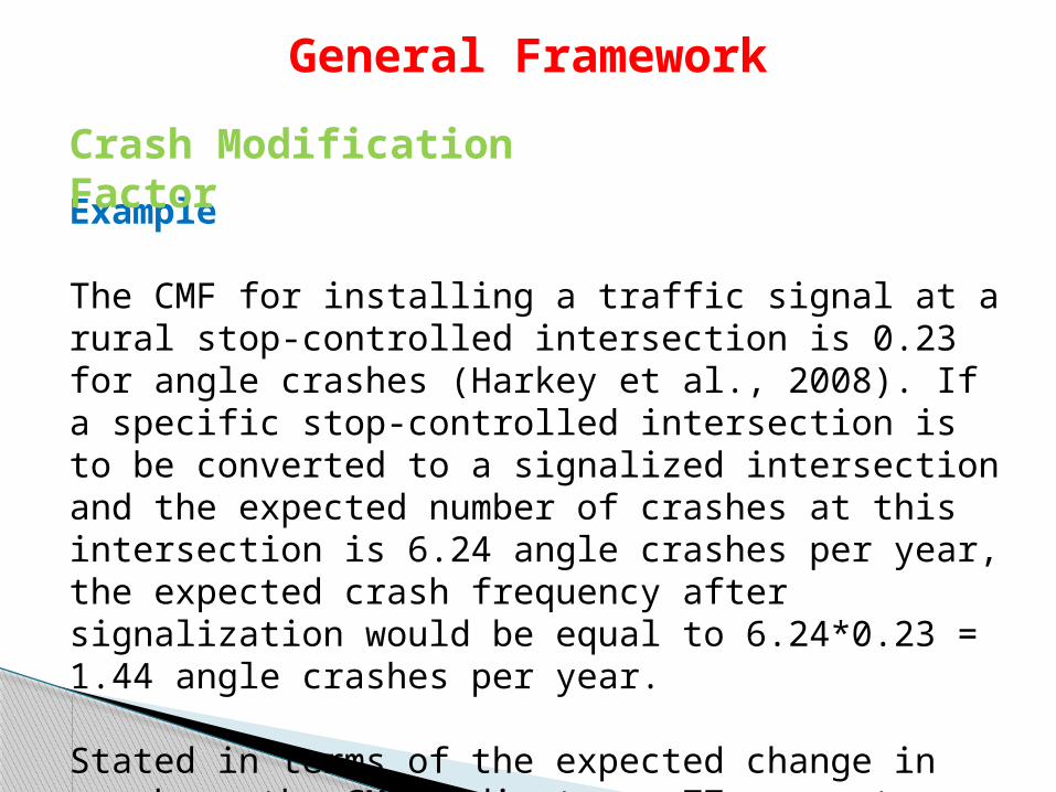
Example

The CMF for installing a traffic signal at a rural stop-controlled intersection is 0.23 for angle crashes (Harkey et al., 2008). If a specific stop-controlled intersection is to be converted to a signalized intersection and the expected number of crashes at this intersection is 6.24 angle crashes per year, the expected crash frequency after signalization would be equal to 6.24*0.23 = 1.44 angle crashes per year.

Stated in terms of the expected change in crashes, the CMF indicates a 77 percent (i.e., 100*(1 – 0.23)) expected reduction in angle crashes after the installation of a traffic signal.

Crash Modification Factor

General Framework

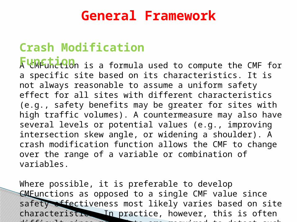
A CMFunction is a formula used to compute the CMF for a specific site based on its characteristics. It is not always reasonable to assume a uniform safety effect for all sites with different characteristics (e.g., safety benefits may be greater for sites with high traffic volumes). A countermeasure may also have several levels or potential values (e.g., improving intersection skew angle, or widening a shoulder). A crash modification function allows the CMF to change over the range of a variable or combination of variables.

Where possible, it is preferable to develop CMFunctions as opposed to a single CMF value since safety effectiveness most likely varies based on site characteristics. In practice, however, this is often difficult since more data are required to detect such differences.

Crash Modification Function

General Framework

Crash Modification Function

General Framework

The standard error is the standard deviation of a sample mean. The standard error provides a measure of certainty (or uncertainty) in the CMF. A relatively small standard error, with respect to the magnitude of the CMF estimate, indicates greater certainty in the estimate of the CMF, while a relatively large standard error indicates less certainty in the estimate of the CMF. The standard error is used in the calculation of the confidence interval. In some cases, the variance of the CMF may be reported instead of the standard error. The standard error is simply the square root of the variance as shown in equation below.

Standard Error

Standard Error = Variance

General Framework

A confidence interval is another measure of the certainty of a CMF. A CMF is simply an estimate of the actual safety effect of a countermeasure based on observations from a sample of sites. The confidence interval provides a range of potential values of the CMF based on the standard error. As the width of the confidence interval increases, there is less certainty in the estimate of the CMF. If the confidence interval does not include 1.0, it can be stated that the CMF is significant at the given confidence level. If, however, the value of 1.0 falls within the confidence interval (i.e., the CMF could be greater than or less than 1.0), it can be stated that the CMF is insignificant at that confidence level. It is important to note insignificant CMFs because the treatment could potentially result in 1) a reduction in crashes, 2) no change, or 3) an increase in crashes. These CMFs should be used with caution (AASHTO, 2010).

Confidence Interval

General Framework

A confidence interval is calculated by multiplying the standard error by a factor (i.e., the cumulative probability) and adding and subtracting the resulting value from the CMF estimate. The equation below is used for calculating the confidence interval.

Confidence Interval = CMF ± (Cumulative Probability * Standard Error)

Confidence Interval

Confidence Interval Cumulative Probability

99% 2.576

95% 1.960

90% 1.645

General Framework

Example

The CMF for a given countermeasure is 0.761 with a standard error of 0.168. An engineer would like to calculate the 95 percent confidence interval for this CMF.

The first step is to determine the appropriate cumulative probability factor from Table 1, given the desired confidence interval. The factor for a 95 percent confidence interval is 1.960. The 95 percent confidence interval is then calculated by adding and subtracting 1.96 times the standard error of 0.168 from the CMF estimate of 0.761.

95% Confidence Interval = 0.761 ± 1.960(0.168)

This gives a confidence interval of 0.432 to 1.090. Note the value of 1.0 lies within the confidence interval. As such, it cannot be stated with 95 percent confidence that the true value of the CMF is not 1.0 (i.e., it cannot be stated with 95 percent confidence that the treatment had any effect).

Crash Modification Factor

General Framework

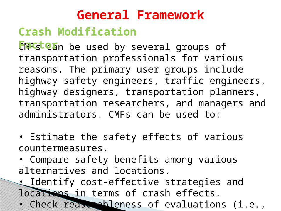
CMFs can be used by several groups of transportation professionals for various reasons. The primary user groups include highway safety engineers, traffic engineers, highway designers, transportation planners, transportation researchers, and managers and administrators. CMFs can be used to:

• Estimate the safety effects of various countermeasures.• Compare safety benefits among various alternatives and locations.• Identify cost-effective strategies and locations in terms of crash effects.• Check reasonableness of evaluations (i.e., compare new analyses with existing CMFs).• Check validity of assumptions in cost-benefit analyses.

Crash Modification Factor

General Framework

/

w

w o

NCMF

N

= expected number of crashes without a treatment or improvement.

CMF is defined as:

/w oN

wN = expected number of crashes with a treatment or improvement.

Note: a number above one implies that an increase in expected number of crashes is observed between sites with treatment and without treatment

General Framework

a bN CMF N

= expected number of crashes after a treatment or improvement is implemented.

Application for single improvement:

aN

bN = expected number of crashes before a treatment or improvement is implemented. (note: also called base condition)

Application for multiple improvements:

1 2 3c nCMF CMF CMF CMF CMF

Note: / 1w oN N CMF

Simple/Naive Before-After Study Before-After Study with Control Group Before-After Study with EB method Cross-sectional study Case-control study Cohort study Meta-Analysis Expert Panel Coefficients of regression models

Methods of Estimation

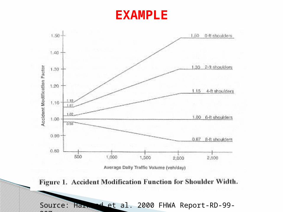
EXAMPLE

Source: Harwood et al. 2000 FHWA Report-RD-99-207

How were units sampled for the study? Do the data collected in the study refer directly to

the outcome of interest or to aggregated data? Was crash or injury severity specified? Were study results tested for statistical

significance or their statistical uncertainty otherwise estimated?

Did the study use appropriate techniques for statistical analysis?

Can the causal direction between treatment and effect be determined?

How well did the study control for confounding factors?

Did the study have a clearly defined target group, and were effects found in the target group only?

Are study results explicable in terms of well-established theory?

Developing CMFs

Evaluation of Design Safety Evaluation of Design Exceptions Evaluation of Design Consistency

Applications in Highway Design

APPLICATIONHighway Design

A 3-mile two-lane rural highway segment linking two cities is being designed. This segment contains one tangent section without any vertical curves. The lane and shoulder widths for the initial proposed design are 12 ft and 5 ft respectively. The traffic volume is estimated at 5,000 vpd. The designer has also identified an alternative design, which consists of having 10-ft lanes with 7-ft shoulders. All other conditions are the same for both designs. Determine the change in safety between the initial and alternative designs.

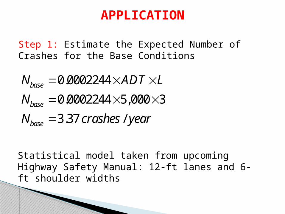
APPLICATION

Step 1: Estimate the Expected Number of Crashes for the Base Conditions

0.0002244

0.0002244 5,000 3

3.37 /

base

base

base

N ADT L

N

N crashes year

Statistical model taken from upcoming Highway Safety Manual: 12-ft lanes and 6-ft shoulder widths

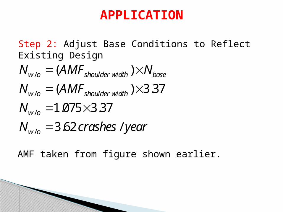
APPLICATION

Step 2: Adjust Base Conditions to Reflect Existing Design

/

/

/

/

( )

( ) 3.37

1.075 3.37

3.62 /

w o shoulder width base

w o shoulder width

w o

w o

N AMF N

N AMF

N

N crashes year

AMF taken from figure shown earlier.

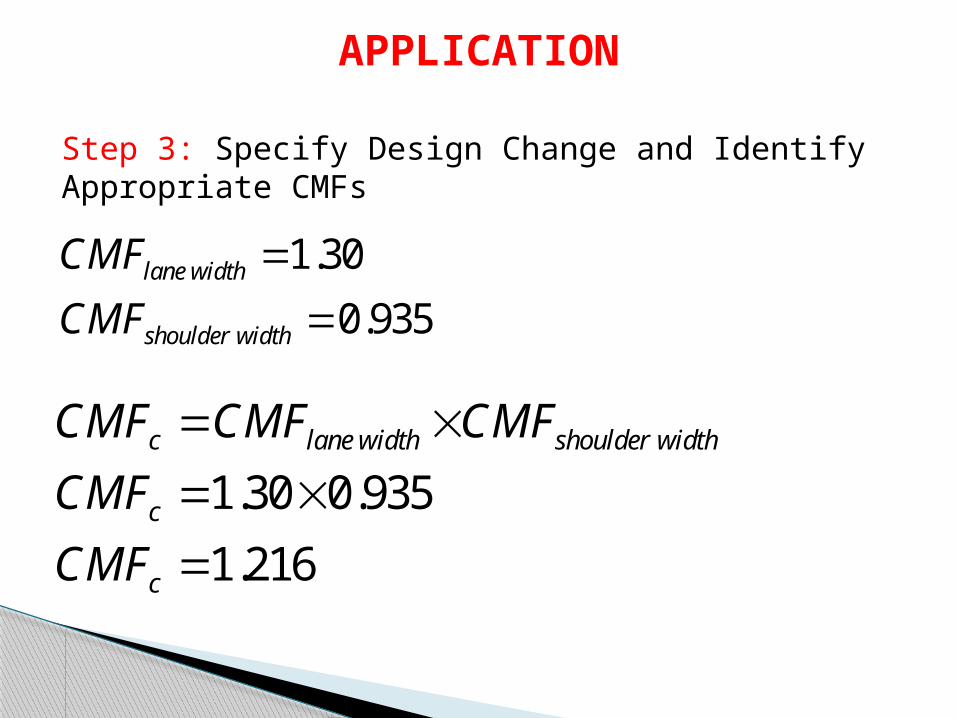
APPLICATION

Step 3: Specify Design Change and Identify Appropriate CMFs

1.30 0.935

1.216

c lane width shoulder width

c

c

CMF CMF CMF

CMF

CMF

1.30

0.935lane width

shoulder width

CMF

CMF

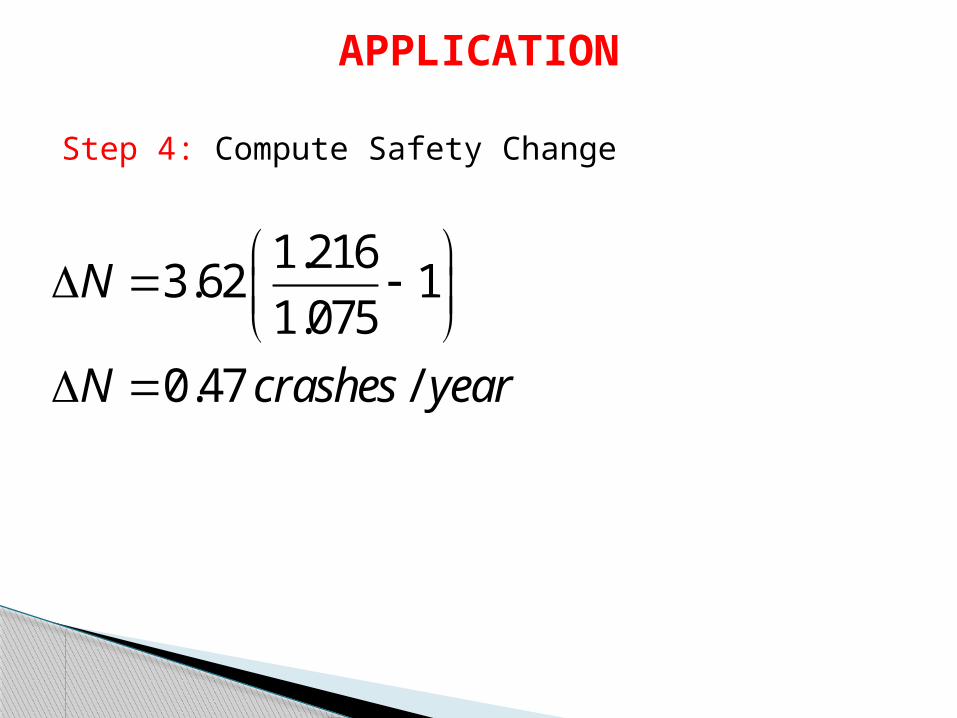
APPLICATION

Step 4: Compute Safety Change

1.2163.62 1

1.075

0.47 /

N

N crashes year

Relationship between CMFs and base conditions◦ CMF is used to adjust for change in condition A to

B◦ The assumption is that B is not represented in the

base model parameter◦ Difficult to determine whether the condition B was

included in the original statistical model

Issues with CMFs

Observed Crash Counts (EB)◦ Not valid for a substantial change in highway

design (between different alternatives)◦ Cannot be used for design exceptions

Combination of Improvements◦ CMFs are assumed to be independent◦ In reality, highway improvements from which

the CMFs are estimated include several design elements changes simultaneously.

◦ In addition, CMFs are probably not independent (shoulder width versus lane width)

Issues with CMFs

Constant versus function◦ Current CMFs are independent of exposure◦ Not true, if we assume a non-linear relationship

between safety and traffic flow Crash Severity and Crash Type

◦ Certain improvements can also influence crash severity or types.

◦ Current CMFs do not consider changes in severity

Issues with CMFs

Crash Migration◦ Def: Interventions influencing crashes at

adjacent sites (note: could also be for different time periods or crash type)

◦ CMFs do not factor in crash migration Statistical Inferences

◦ Most research do not provide confidence intervals

◦ High uncertainty/high reduction versus low uncertainty/low reduction

◦ Now, researchers have started to provide information about the variance.

Expert Panels/Meta-Analysis◦ Subjective estimation (panel)◦ Panel does not know characteristics of data

(both)◦ No confidence intervals available (panel)

Issues with CMFs

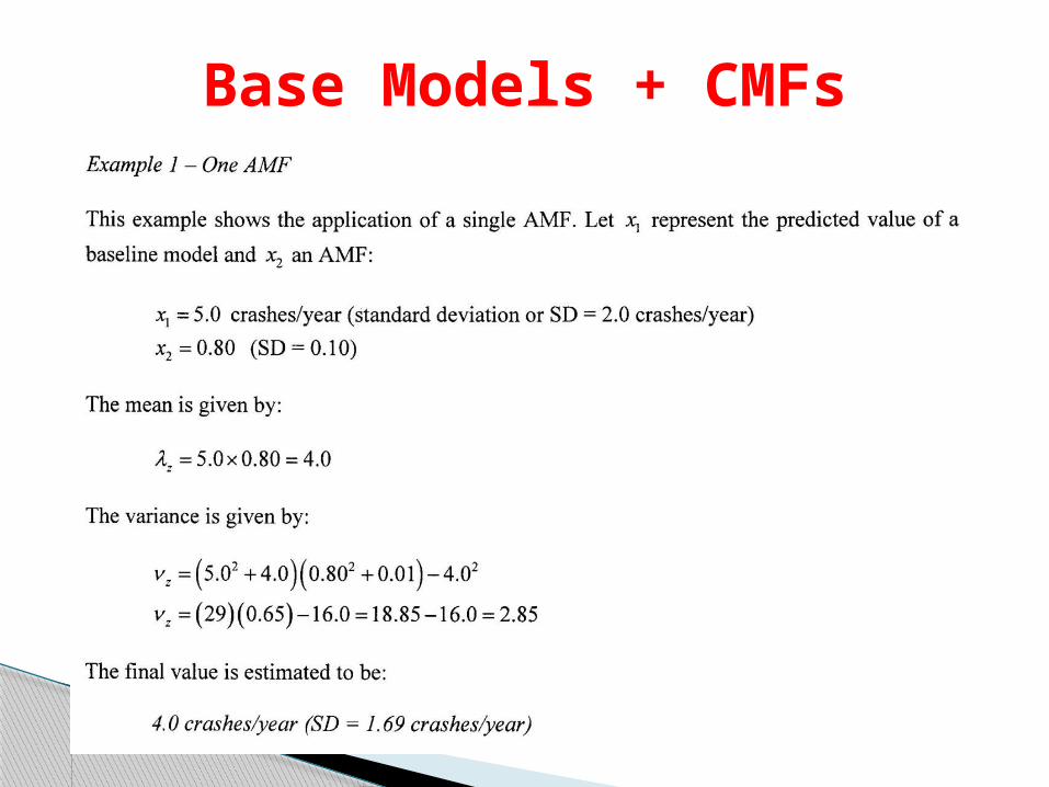
Base Models + CMFsCalculating the variance for the product of SPFs + CMFs

Based on the theory of Independent Random Variables 321 xxxz

z

sx'

where,

= the product of independent random variables; and,

= random variable taken from any kind of distribution.

E x 2E x

It should be pointed out that the mean and variance estimates are defined as

and (second central moment), respectively.

See Lord, D. (2008) Methodology for Estimating the Variance and Confidence Intervals of the Estimate of the Product of Baseline Models and AMFs. Accident Analysis & Prevention, Vol. 40, No. 3, pp. 1013-1017.

Base Models + CMFsMean of a Product

321 xxxz 321 xExExEzE

1 2 3z x x x

Base Models + CMFsVariance of a Product

23

22

21

2 xxxz

23

22

21

2 xExExEzE

2 2 2 21 1 2 2 3 3z z x x x x x x

nnE x E x Note:

2n

22E x E x 2 2 22E x E x E

for

Base Models + CMFs

Base Models + CMFs

Base Models + CMFs

Base Models + CMFs

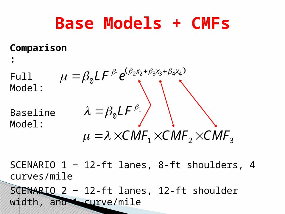
2 2 3 3 4 410

x x xLF e

10LF

Comparison:

SCENARIO 1 − 12-ft lanes, 8-ft shoulders, 4 curves/mile

SCENARIO 2 − 12-ft lanes, 12-ft shoulder width, and 1 curve/mile

Full Model:

Baseline Model:

1 2 3CMF CMF CMF

Base Models + CMFsComparison – Scenario 1 (KAB):

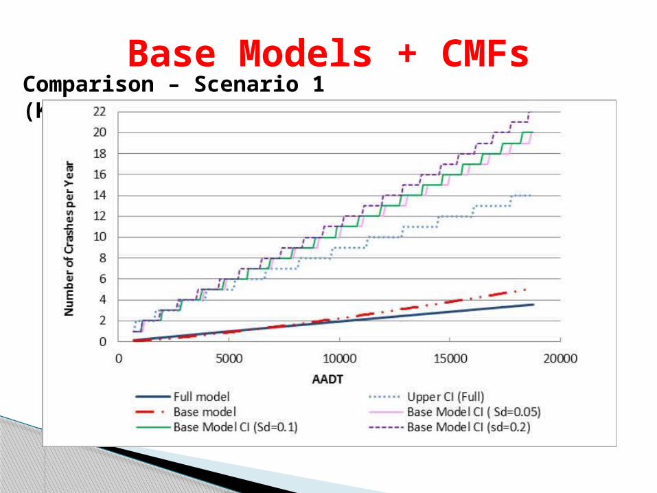
Base Models + CMFsComparison – Scenario 1 (KABCO):

Base Models + CMFsComparison – Scenario 2 (KAB):

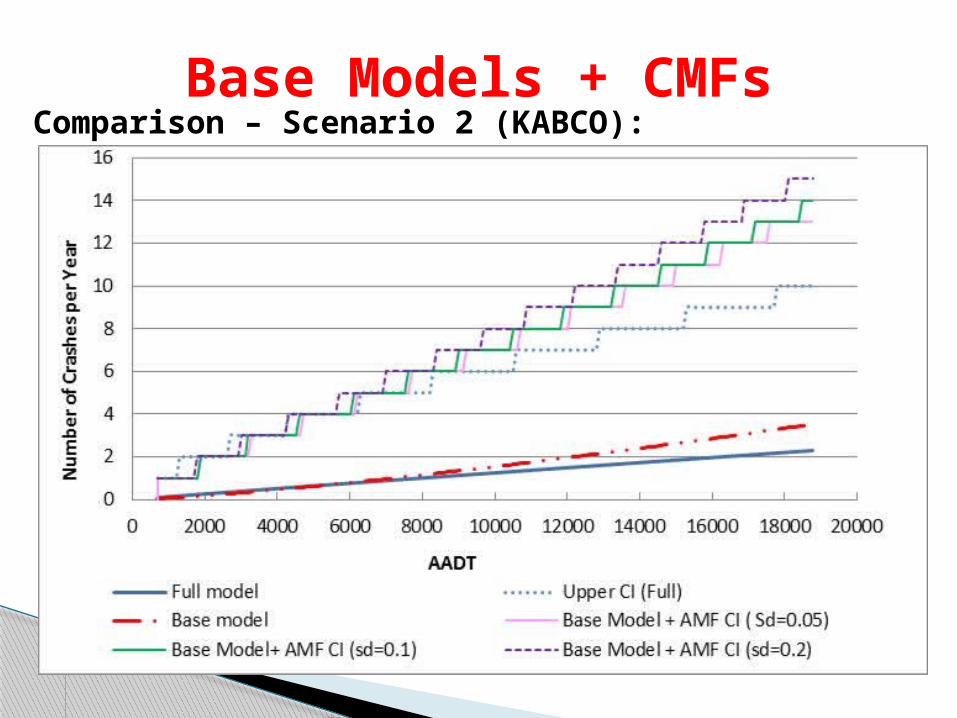
Base Models + CMFsComparison – Scenario 2 (KABCO):

Base Models + CMFsComparison

Lord, D., P.-F. Kuo, and S.R. Geedipally (2010) Comparing the Application of the Product of Baseline Models and Accident Modification Factors and Models with Covariates: Predicted Mean Values and Variance. Transportation Research Record 2147, pp. 113-122.