Embed Size (px)
DESCRIPTION
Libro interactivo para mejorar las aplicaciones de excel en el área de finanzas y la programación para la simulación de eventos.
Citation preview

7/18/2019 SpreadsheetGuide_1.02 (1) - copia
http://slidepdf.com/reader/full/spreadsheetguide102-1-copia 1/114
Spreadsheet Skills and Modelling
[* Comments related to interactivity in this text relate to the spreadsheet version of this guide]
These are the book's goals:
-
-
- To let the reader test their mastery of the spreadsheet functions described in this book by carrying out a set of exercises.
The layout of this book is as follows.
Chapter 1
Interactive sections are marked by colours. Cells with a blue background that look like this .!"# the reader can change.
Chapter 2
Chapter 3
Chapter 4
Chapter 5
This chapter gives you links to our on-line resources whereby you can further advance your spreadsheet skills.
About this book
- $age % - &ack to top
Copyright c( )""* Tykoh +roup $ty ,imited
www.tykoh.com
1.02
- free interactive/( guide
This guide is available in two forms: s a spreadsheet and as a $01 document. 2f the two versions the more useful and interesting one is thespreadsheet 3,4(: The $01 version is a book but the spreadsheet version is an interactive book.
To show the reader examples of the things that are possible with spreadsheets. 4urprisingly there are very few compilations like this of a setof wide-ranging and consistently presented spreadsheet examples.
To allow the reader to master some of the most important spreadsheet functions. The guide explains how important functions work and givesexamples of how they can be used.
Chapter % presents a set of spreadsheet applications. The applications are broad in scope some are fairly basic and others are more complex.Their purpose is to illustrate many of the capabilities - some of them not well known - of spreadsheets. lmost all of the examples are interactive.
t the end of the chapter is a cross reference that lists the spreadsheet functions and features used in the earlier examples. The cross referenceshows that even 5uite complex applications often use only a small number of spreadsheet functions an average of eight - in our examples(. crossall of the examples in this chapter seven out of eight spreadsheet functions are never used. Important insights flow from this: %( 6astery ofspreadsheets re5uires knowledge about a relatively small subset of spreadsheet functions )( 6ost other functions can be ignored.
6ost things that are complex are built from a set of simple and fundamental components. That's true also with spreadsheets. 7ach example in thepreceding chapter was made by choosing about 8 functions from a set of 9".
In this chapter we look at the building blocks of spreadsheets - the individual functions that can be combined to make complex applications. ;edescibe what the functions do how they are used and give examples of their applications.
Individual spreadsheet functions - as described in the preceding chapter - serve specific and usually simple purposes. &ut what if we want to dosomething that an individual function can't< Then we need to combine two or more functions - in effect to design a super-function. The morefunctions you need to combine - the harder this is to do. In this chapter we take first steps in this design process - by combining two or threefunctions to build mini-applications.
=aving completed the earlier chapters you are now in a position to test your design skills in a more open-ended environment. >ou are given a set ofproblems to solve and you need to work out which functions to use and how to combine them to solve the problems.
This book is aimed at those with intermediate levels of skills in spreadsheets - it is not a beginner's book. The concepts examples and exercisesrange from intermediate to advanced levels. s with other free works on the internet some advertising is included. The advertising relates toworkshops we run and services we offer.
+ood luck? ;e hope you find this guide useful in increasing your expertise with spreadsheets and their applications. If at some stage you areinterested in attending a spreadsheet or financial modelling workshop please consider the ones we offer. lso please tell those you know who areinterested in spreadsheets about this guide and our workshops.
Disclaimer: y!oh "roup #ty $imited %&y!oh&' disclaims all (arranties of )uality accuracy correctness or fitness for a particular purpose. he user assumes the entire ris! as to the)uality accuracy and correctness of this (or!. he user assumes the entire ris! as to conse)uences of any actions user may ta!e or not ta!e as a result of anything in this (or!. +n noevent (ill y!oh ,e lia,le for any indirect special or conse)uential damages. his (or! may not ,e modified in any (ay nor may any attempt ,e made to unloc! unprotect reverseengineer or include it as part of any other (or!. his (or! may ,e freely distri,uted for private individual use. his (or! may not ,e used for teaching purposes (ithout the prior (ritten
permission of y!oh. -ll rights reserved.
7/18/2019 SpreadsheetGuide_1.02 (1) - copia
http://slidepdf.com/reader/full/spreadsheetguide102-1-copia 2/114
Contents
%
)
Chapter 1 - Sample Spreadsheet Applications
!
9
@
A
8
*
%"
%%
%)
%!
%9
%@%
%A
%8
%*
)"
)"
Chapter 2 - Functions
)%
))
)!
)9
)@
)
)A
)8
)*
!"
!"
!%
!)
!!
!"
!!
!9
))
!"
!@
!!A
Chapter 3 - Combining Functions
Buartiles !8
Complex counting !*
)0 lookups 9"
9%
Chapter 4 - Exercises
Compound I1 functions 9)
Conditional counting 9!
Tracking cashflows 99
Interpolating 9@
Complex lookups 9
9A
Chapter 5 - Next steps
98
ndex
9*
&ack to contents - $age ! - &ack to top
Copyright c( )""* Tykoh +roup $ty ,imited
www.tykoh.com
ntroduction
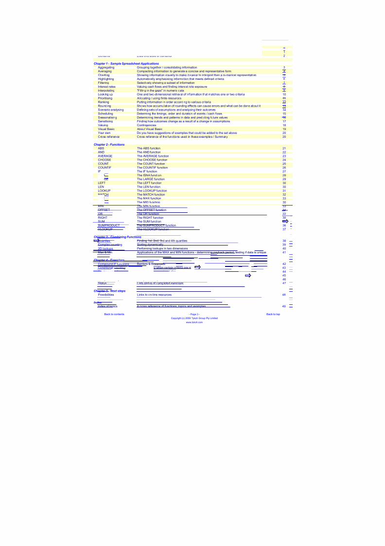
2verview +ives an overview of this book - its purpose format and use
Contents ,ists this table of contents
ggregating +rouping together consolidating information
veraging Compacting information to generate a concise and representative form
Charting 4howing information visual ly to make i t easier to interpret than a numerical representation
=ighlighting utomatically emphasising information that meets defined criteria
1iltering 4electively showing a subset of information
Interest rates Daluing cash flows and finding interest rate exposure
Interpolating 1illing in the gaps in numeric data
,ooking up 2ne and two-dimensional retrieval of information that matches one or two cr iteria
$rioritising llocating using finite resources
Eanking $utting information in order according to various criteria
Eounding 4hows how accumulation of rounding effects can cause errors and what can be done about it
4cenario analysing 0efining sets of assumptions and analysing their outcomes
4cheduling 0eterming the timings order and duration of events cash flows4easonal ising 0etermining trends and patterns in data and predicting future values
4ensitising 1inding how outcomes change as a result of a change in assumptions
Daluing Contingencies
Disual &asic bout Disual &asic
>our own 0o you have suggestions of examples that could be added to the set above
Cross reference Cross reference of the functions used in these examples 4ummary
&4 The &4 function
F0 The F0 function
D7E+7 The D7E+7 function
C=2247 The C=2247 function
C2GFT The C2GFT function
C2GFTI1 The C2GFTI1 function
I1 The I1 function
I4F The I4F function
,E+7 The ,E+7 function
,71T The ,71T function
,7F The ,7F function
,22HG$ The ,22HG$ function
6TC= The 6TC= function
63 The 63 function
6I0 The 6I0 function
6IF The 6IF function
21147T The 21147T function
2E The 2E function
EI+=T The EI+=T function
4G6 The 4G6 function
4G6$E20GCT The 4G6$E20GCT functionD,22HG$ The D,22HG$ function
1inding %st )nd !rd and 9th 5uartiles
4orting dynamically
$erforming lookups in two dimensions
6ax 6in pplications of the 63 and 6IF functions - determining payback period testing if data is uni5ue
&arriers thresholds
Counting only when certain criteria are met
0etermining amount and direction of cashflows
Interpolating to fill in gaps in data
Complex lookups
4tatus ,ists status of completed exercises
$ossibilities ,inks to on-line resources
Index of topics cross reference of functions topics and examples

7/18/2019 SpreadsheetGuide_1.02 (1) - copia
http://slidepdf.com/reader/full/spreadsheetguide102-1-copia 3/114
Chapter 1 - Sample Spreadsheet Applications
In this chapter - and elsewhere in this guide also - we use a colour convention to indicate which cells you can change.
Cells that have a blue background and white text can be changed by you. Those cells look like this: .!"#
Aggregating
Spreadsheet functions used in this example
Conditional format I1 ,7F 63 6IF 4G6$E20GCT
Transaction data
0ate Code mount 0ate Code mount 0ate Code mount
)-4ep 0II-!9 !.A9 )-4ep 70-@! 8.*8 )-4ep &IC-!" *9.@9 A
A-2ct =7J-% !.*) )8-Fov =11-*" )@.*! %9-2ct =+-8% 8*."% %9
-Fov J1+-A) 8!.") )-Fov ICC-) 9.A9 )-Fov J=C-)9 9*.* )8
)@-2ct =+0-*8 ).!" %9-4ep I=7-)@ @).A@ )@-Fov 11&-!A AA.@) %
%)-Fov &I&-AA )9." A-4ep +I7-!@ [email protected] %8-2ct C+J-!! 9@."8 9@."8
)-Fov 0C-@8 8".*! %%-2ct C-" %9."A )@-4ep 1CI-89 @.%" @.%"
%"-2ct 170-%A *.@8 %@-Fov CJ1-!) 99."% %@-Fov ==7-*A @8.
%9-4ep 1+0-)8 )8.%@ %%-Fov 7+7-!! *%.!8 %%-Fov &0-8" 8A.!)%-2ct 7I0-* A*.88 8-2ct C0-A9 8%.8@ ))-4ep =C+-!! 88."A
ggegation grouping( interval
+rouping interval days( A KF67<
ggegated results
9 ) % % - 9 ! % - % @ - @ -
)-4ep *-4ep %-4ep )!-4ep !"-4ep A-2ct %9-2ct )%-2ct )8-2ct 9-Fov %%-Fov %8-Fov )@-Fov )-0ec8-4ep %@-4ep ))-4ep )*-4ep -2ct %!-2ct )"-2ct )A-2ct !-Fov %"-Fov %A-Fov )9-Fov %-0ec 8-0ec
&ack to contents - $age ! - &ack to top
Copyright c( )""* Tykoh +roup $ty ,imited
www.tykoh.com
Attend one of our workshops andlearn how to use a wide range of
spreadsheet functions in practical finance settings
&usiness and finance activities can often be described in terms of processes. process is a set of actionsperformed on some input to generate an output. &usiness and finance processes could involve aggregating
summarising reporting valuing filtering prioritising ranking etc. In this chapter we look at examples of suchbusiness processes and show how they can be represented and implemented in spreadsheets.
The applications shown here have a finance emphasis but most can e5ually well be applied outside of the finance area. 7ach example lists thespreadsheet functions and features that were used to build the example. t the end of the chapter we review the spreadsheet functions andfeatures used in the examples and draw some conclusions from those.
vervie! ggregating involves grouping together or consolidating information. In the following example we aggregate transactions by grouping them into dateintervals. ;e then show the number of transactions that occurred in each interval. The number of transactions is shown graphically - but in asomewhat unusual way - rather than using a chart we use conditional formatting.
We specialise in presenting oneand two day finance / technical
workshops
F u m b e r o f
t r a n s a c t i o n s i n
i n t e r v a l
7/18/2019 SpreadsheetGuide_1.02 (1) - copia
http://slidepdf.com/reader/full/spreadsheetguide102-1-copia 4/114
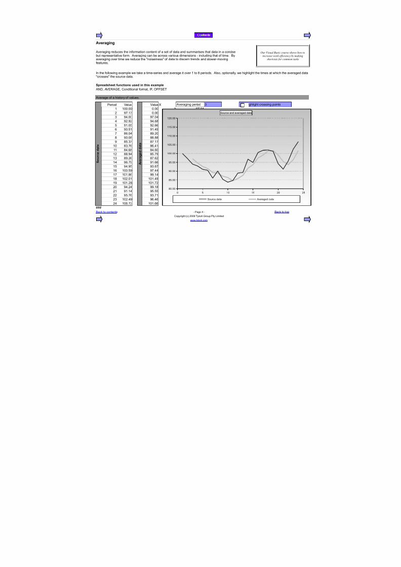
Averaging
Spreadsheet functions used in this example
F0 D7E+7 Conditional format I1 21147T
verage of a history of values.
S o u r c e d a t a
$eriod Dalue
A v e r a g e d d a t a
Dalue 3 veraging period ! =ighlight crossing points
% %""."" "."" ! *A."9
) *A.%! "."" ! *A."9
! *9."" *A."9 ! *A."99 *).*) *9.8 9 *9.8 "
@ *%."@ *). @ *). KF67<
*".@% *%.9* *%.9*
A 8."9 8*.)" A 8*.)"
8 *"."8 88.88 8 88.88
* 8@.!A 8A.%A * 8A.%A
%" 8!.A 8.9% %" 8.9%
%% 89.8 89." %% 89."
%) 88.*9 [email protected]* %) [email protected]*
%! 8*.) 8A.) %! 8A.)
%9 *.A* *%. %9 *%.
%@ *9.*@ *!.A %@ *!.A
% %"".@* *A.99 % *A.99
%A %"%.8 **.%9 %A **.%9%8 %")."% %"%.9* %8 %"%.9*
%* %"%.)8 %"%.A) %* %"%.A)
)" *9.)9 **.%8 )" **.%8
)% *%.%9 *@.@@ )% *@.@@
)) *@.A *!.A% )) *!.A%
)! %").9* *.9 )! *.9
)9 %".A) %"%. )9 %"%.
KKK
&ack to contents - $age 9 -
Copyright c( )""* Tykoh +roup $ty ,imited
www.tykoh.com
Our Visual Basic course shows how toincrease work efficiency by making
shortcuts for common tasks
veraging reduces the information content of a set of data and summarises that data in a concisebut representative form. veraging can be across various dimensions - including that of time. &y
averaging over time we reduce the noiseiness of data to discern trends and slower-movingfeatures.
In the following example we take a time-series and average it over % to 8 periods. lso optionally we highlight the times at which the averaged datacrosses the source data.
&ack to top
" @ %" %@ )" )@
8".""
8@.""
*".""
*@.""
%"".""
%"@.""
%%".""
%%@.""
%)".""
4ource and averaged data
4ource data veraged data
7/18/2019 SpreadsheetGuide_1.02 (1) - copia
http://slidepdf.com/reader/full/spreadsheetguide102-1-copia 5/114
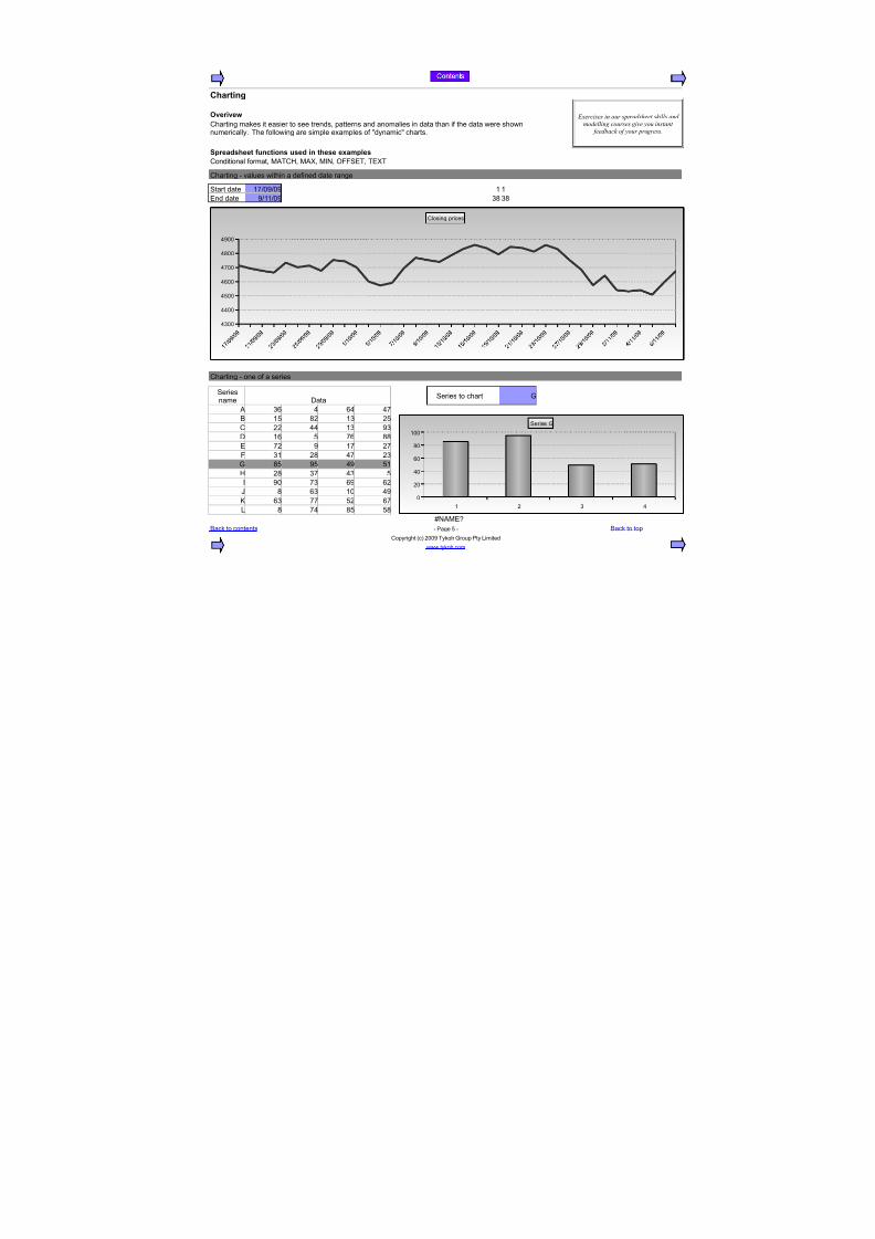
Charting
verive!
Spreadsheet functions used in these examples
Conditional format 6TC= 63 6IF 21147T T73T
Charting - values within a defined date range
4tart date %A"*"* % %
7nd date *%%"* !8 !8
Charting - one of a series
0ata 4eries to chart +
! 9 9 9A
& %@ 8) %! )@
C )) 99 %! *! 8@ *@ 9* @%
0 % @ A 88 index
7 A) * %A )A
1 !% )8 9A )! 4eries +
+ 8@ *@ 9* @%
= )8 !A 9! @
I *" A! * )
J 8 ! %" 9*
H ! AA @) A
, 8 A9 8@ @8 KF67<
&ack to contents - $age @ - &ack to top
Copyright c( )""* Tykoh +roup $ty ,imited
www.tykoh.com
Exercises in our spreadsheet skills andmodelling courses give you instant
feedback of your progressCharting makes it easier to see trends patterns and anomalies in data than if the data were shownnumerically. The following are simple examples of dynamic charts.
4eriesname
9!""
99""
9@""
9""
9A""
98""
9*""
Closing prices
% ) ! 9
"
)"
9"
"
8"
%""
4eries +
7/18/2019 SpreadsheetGuide_1.02 (1) - copia
http://slidepdf.com/reader/full/spreadsheetguide102-1-copia 6/114
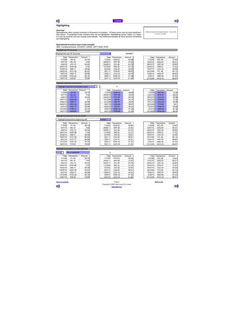
"ighlighting
Spreadsheet functions used in this example
F0 Conditional format C2GFTI1 ,E+7 ,71T 620 E2;
=ighlight top F amounts
=ighlight the top F amounts: " KF67<
0ate Transaction mount 0ate Transaction mount 0ate Transaction mount
%%)"* 0II-!9 !.A9 %%)"* 70-@! 8.*8 %%)"* &IC-!" %9.@9
@"%%" =7J-% !.*) )")%" =11-*" )@.*! %)"%%" =+-8% 8*."%
9")%" J1+-A) 8!.") )9")%" ICC-) 9.A9 )9")%" J=C-)9 9*.*
)!"%%" =+0-*8 ).!" %!%)"* I=7-)@ @).A@ )!")%" 11&-!A AA.@)
%"")%" &I&-AA *9." %)"* +I7-!@ [email protected] %"%%" C+J-!! 9@."8)9")%" 0C-@8 8".*! *"%%" C-" *@.A )9%)"* 1CI-89 @.%"
8"%%" 170-%A *.@8 %!")%" CJ1-!) 99."% %!")%" ==7-*A @8.
%!%)"* 1+0-)8 )8.%@ *")%" 7+7-!! *%.!8 *")%" &0-8" 8A.!)
%9"%%" 7I0-* A*.88 "%%" C0-A9 8%.8@ )%%)"* =C+-!! 88."A
=ighlight duplicate transactions
=ighlight duplicate transaction codes "
0ate Transaction mount 0ate Transaction mount 0ate Transaction mount
%%)"* 0II-!9 !.A9 %%)"* 70-@! 8.*8 %%)"* &IC-!" %9.@9
@"%%" =7J-% !.*) )")%" =11-*" )@.*! %)"%%" =+-8% 8*."%
9")%" J1+-A) 8!.") )9")%" ICC-) 9.A9 )9")%" J=C-)9 9*.*
)!"%%" =+0-*8 ).! %!%)"* 0II-!9 @).A@ )!")%" 11&-!8 AA.@)
%"")%" &I&-AA *9." %)"* +I7-!@ [email protected] %"%%" C+J-!! 9@."8)9")%" 0C-@8 8".*! *"%%" C-" *@.A )9%)"* 1CI-89 @.%
8"%%" 170-%A *.@8 %!")%" 0II-!9 99."% %!")%" ==7-*A @8.
%!%)"* 11&-!A )8.%@ *")%" 7+7-!! *%.!8 *")%" &0-8" 8A.!)
%9"%%" 7I0-* A*.88 "%%" 11&-!8 8%.8@ )%%)"* =C+-!! 88."A
=ighlight transactions that are similar
=ighlight transactions beginning with LnoneM
0ate Transaction mount 0ate Transaction mount 0ate Transaction mount
%%)"* 0II-!9 !.A9 %%)"* 70-@! 8.*8 %%)"* &IC-!" %9.@9
@"%%" =7J-% !.*) )")%" =11-*" )@.*! %)"%%" =+-8% 8*."%
9")%" J1+-A) 8!.") )9")%" ICC-) 9.A9 )9")%" J=C-)9 9*.*
)!"%%" =+0-*8 ).!" %!%)"* I=7-)@ @).A@ )!")%" 11&-!A AA.@)
%"")%" &I&-AA *9." %)"* +I7-!@ [email protected] %"%%" C+J-!! 9@."8
)9")%" 0C-@8 8".*! *"%%" C-" *@.A )9%)"* 1CI-89 @.%"8"%%" 170-%A *.@8 %!")%" CJ1-!) 99."% %!")%" ==7-*A @8.
%!%)"* 1+0-)8 )8.%@ *")%" 7+7-!! *%.!8 *")%" &0-8" 8A.!)
%9"%%" 7I0-* A*.88 "%%" C0-A9 8%.8@ )%%)"* =C+-!! 88."A
=ighlight transactions on alternate lines
4how highlights "
0ate Transaction mount 0ate Transaction mount 0ate Transaction mount
%%)"* 0II-!9 !.A9 %%)"* 70-@! 8.*8 %%)"* &IC-!" %9.@9
@"%%" =7J-% !.*) )")%" =11-*" )@.*! %)"%%" =+-8% 8*."%
9")%" J1+-A) 8!.") )9")%" ICC-) 9.A9 )9")%" J=C-)9 9*.*
)!"%%" =+0-*8 ).!" %!%)"* I=7-)@ @).A@ )!")%" 11&-!A AA.@)
%"")%" &I&-AA *9." %)"* +I7-!@ [email protected] %"%%" C+J-!! 9@."8
)9")%" 0C-@8 8".*! *"%%" C-" *@.A )9%)"* 1CI-89 @.%"
8"%%" 170-%A *.@8 %!")%" CJ1-!) 99."% %!")%" ==7-*A @8.
%!%)"* 1+0-)8 )8.%@ *")%" 7+7-!! *%.!8 *")%" &0-8" 8A.!)
%9"%%" 7I0-* A*.88 "%%" C0-A9 8%.8@ )%%)"* =C+-!! 88."A
&ack to contents - $age - &ack to top
Copyright c( )""* Tykoh +roup $ty ,imited
www.tykoh.com
Outsourcing of training functions ! one of the
services we offer
vervie!4preadsheets often contain hundreds or thousands of numbers. 2f those some may be more signficant
than others. To emphasis those numbers they can be highlighted. =ighlighting can be static i.e. fixed(or it can be dynamic and can change automatically. The following examples all show dynamic formattingand highlighting.

7/18/2019 SpreadsheetGuide_1.02 (1) - copia
http://slidepdf.com/reader/full/spreadsheetguide102-1-copia 7/114
#iltering
Spreadsheet functions used in this example
F0 I1 I4F 6TC= 63 6IF 21147T 4G6
4ource - unfiltered - data
0ate Transaction mount 0ate Transaction mount 0ate Transaction mount
%%)"* 0II-!9 !.A9 %%)"* 70-@! 8.*8 %%)"* &IC-!" *9.@9
@"%%" =7J-% !.*) )")%" =11-*" )@.*! %)"%%" =+-8% 8*."%
9")%" J1+-A) 8!.") )9")%" ICC-) 9.A9 )9")%" J=C-)9 9*.*
)!"%%" =+0-*8 ).!" %!%)"* I=7-)@ @).A@ )!")%" 11&-!A AA.@)
%"")%" &I&-AA )9." %)"* +I7-!@ [email protected] %"%%" C+J-!! 9@."8
)9")%" 0C-@8 8".*! *"%%" C-" %9."A )9%)"* 1CI-89 @.%"
8"%%" 170-%A *.@8 %!")%" CJ1-!) 99."% %!")%" ==7-*A @8.
%!%)"* 1+0-)8 )8.%@ *")%" 7+7-!! *%.!8 *")%" &0-8" 8A.!)%9"%%" 7I0-* A*.88 "%%" C0-A9 8%.8@ )%%)"* =C+-!! 88."A
1iltering criteria
4how transaction that have values between 8" and @"
1iltered data
0ate Transaction Dalue 0ate Transaction Dalue 0ate Transaction Dalue
8"%%" 170-%A *.@8 %%)"* 70-@! 8.*8 )!")%" 11&-!A AA.@)
%9"%%" 7I0-* A*.88 )9")%" ICC-) 9.A9 )9%)"* 1CI-89 @.%"
%!%)"* I=7-)@ @).A@ %!")%" ==7-*A @8.
&ack to contents - $age A - &ack to top
Copyright c( )""* Tykoh +roup $ty ,imited
www.tykoh.com
Our Visual Basic course shows how to automateroutine work and save the time and trouble of
doing the same thing over and over
vervie!2n occasion we may want to focus on subsets of data rather than the whole data set. In other words - we
may want to filter the data and see only the filtered result. The following is a simple example.
7/18/2019 SpreadsheetGuide_1.02 (1) - copia
http://slidepdf.com/reader/full/spreadsheetguide102-1-copia 8/114
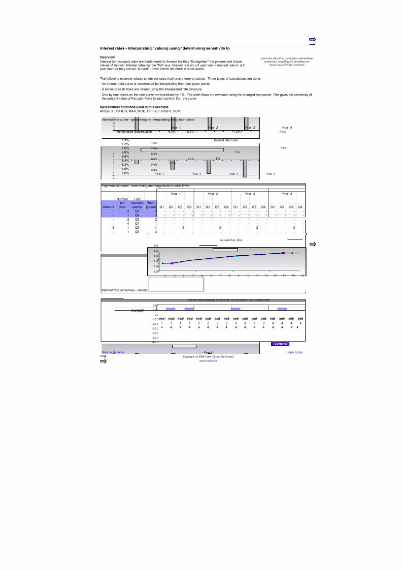
$nterest rates % $nterpolating & valuing using & determining sensitivit' to
vervie!
The following example relates to interest rates that have a term structure. Three types of calculations are done:
- n interest rate curve is constructed by interpolating from four given points.
- series of cash flows are valued using the interpolated rate structure.
-
Spreadsheet functions used in this example
rrays I1 6TC= 63 620 21147T EI+=T 4G6
Interest rate curve - generating by interpolating using four points
>ear % >ear ) >ear ! >ear 9Interest rates Nero coupon(: ."# .9# A."# A.9#
A.9#
A.)#
A."#
.8#
.#
.9#
.)#
."#
@.8#
$ayment schedule - sets t iming and magnitude of cash flows
>ear % >ear ) >ear ! >ear 9
Term
mount year 5uarter years( B% B) B! B9 B% B) B! B9 B% B) B! B9 B% B) B! B9
- ) B% 9 - - - - - - - - - - - - - - - -
- % B9 9 - - - - - - - - - - - - - - - -
- ) B! ) - - - - - - - - - - - - - - - -
- 9 B% % - - - - - - - - - - - - - - - -
) % B! 9 - - ) - - - ) - - - ) - - - ) -
- % B! ) - - - - - - - - - - - - - - - -
Interest rate sensitivity - calculation of sensitivity of cash flow value to each point on the rate curve
KF67<
KKK KKK KKK KKK KKK KKK KKK KKK KKK KKK KKK KKK KKK KKK KKK KKK
% % % % ) ) ) ) ! ! ! ! 9 9 9 9
9 9 9 9 9 9 9 9 9 9 9 9 9 9 9 9
"earn the ob#ectives$ principles and methodsof financial modelling by attending our
financial modelling workshopInterest or discount( rates are fundamental in finance for they tie together the present and futurevalues of money. Interest rates can be flat e.g. interest rate on a ) year loan O interest rate on a @year loan( or they can be curved - have a term structure in other words.
2ne by one points on the rate curve are increased by %#. The cash flows are revalued using the changed rate points. This gives the sensitivity ofthe present value of the cash flows to each point in the rate curve.
Fumberper
1irstpayment
>ear % >ear ) >ear ! >ear 9
@."#
@.@#
."#
.@#
A."#
A.@#
A.9#
A."#
.9#
."#
Interest rate curve
% ) ! 9 @ A 8 * %" %% %) %! %9 %@ %
-"."
-@"."
-9"."
-!"."
-)"."
-%"."
"."
%"."
)"."
Interest rate sensitivity P"""'s per %# increase in Nero coupon rate(
% ) ! 9 @ A 8 * %" %% %) %! %9 %@ %
".""
".@"
%.""
%.@"
).""
).@"
Fet cash flow Pm(

7/18/2019 SpreadsheetGuide_1.02 (1) - copia
http://slidepdf.com/reader/full/spreadsheetguide102-1-copia 9/114
$nterpolating
Spreadsheet functions used in these examples
IFT ,22HG$ 6TC= 6IFD7E47 66G,T 21147T T73T TE7F0
4tepped interpolation as is done by ,22HG$ D,22HG$ and =,22HG$(
+nterpolation ta,le
x y
" -)
% -!
) )
! %
9 !
3 value to interpolate !.@
;hen 3 is !.@" > is %.""
$iecewise linear interpolation. combination of functions is needed to achieve this.
+nterpolation ta,le
x y
" -)
% -!
) )
! %
9 !
3 value to interpolate !.@
;hen 3 is !.@" > is ).""
Cubic spline interpolation. combination of functions is needed to achieve this.
+nterpolation ta,le
x y
" -)
% -!
) )
! %
9 !
3 value to interpolate !.@
;hen 3 is !.@" > is %.@"
4tatistical - line of best fit - interpolation
Data points
x y
" -)
% -!
) )
! %
9 !
3 value to interpolate !.@
;hen 3 is !.@" > is ).!"
&ack to contents - $age * - &ack to top
Copyright c( )""* Tykoh +roup $ty ,imited
www.tykoh.com
Our Visual Basic course shows how to
increase the %wow!factor% of your developedapplications
vervie!
Interpolating involves filling in the gaps in numeric data. The examples below all use the same data set.Fote that even with the same data set different interpolation methods can give significantly different answers.;hich is the correct answer< The appropriate method to use depends on the context.
"." ".@ %." %.@ )." ).@ !." !.@ 9."
-!.@
-).@
-%.@
-".@
".@
%.@
).@
!.@
;hen 3 is !.@" > is ).""
3
>
"." ".@ %." %.@ )." ).@ !." !.@ 9."
-!.@
-).@
-%.@
-".@
".@
%.@
).@
!.@ ;hen 3 is !.@" > is %.@"
3
>
"." ".@ %." %.@ )." ).@ !." !.@ 9."
-!.@
-).@
-%.@
-".@
".@
%.@
).@
!.@
;hen 3 is !.@" > is %.""
3
>
"." ".@ %." %.@ )." ).@ !." !.@ 9."
-!.@
-).@
-%.@
-".@
".@
%.@
).@
!.@
;hen 3 is !.@" > is ).!"
3
>

7/18/2019 SpreadsheetGuide_1.02 (1) - copia
http://slidepdf.com/reader/full/spreadsheetguide102-1-copia 10/114
(ooking up
Spreadsheet functions used in this example
F0 rrays Conditional format 6TC= 63 6IF 4G6$E20GCT D,22HG$
)0 lookup K%
200 200/ 200 200 200
3an @ @@ 9 8 9A
4e, )) %8 * 8A %)
5ar 98 *! 9* %
6onth to look up 2ct -pr %A %! !8 @9 %
>ear to look up )""8 5ay A" @9 8" * *A
3un !! A 89 *9 9"
nswer A) 3ul 8 !9 !" ! *!
-ug *% )* 9 %9 9A
6ep % A% 8A !8 !%
7ct 9% !8 * A) )*
8ov @9 @ )" ** 9!
Dec @ !9 A" *9
)0 lookup K)
200 200/ 200 200 200 *!
3an @ @@ 9 8 9A %%)
4e, )) %8 * 8A %)
5ar 98 *! 9* % *! -pr %A %! !8 @9 % %%)
5ay A" @9 8" * *A
4tart month to look up 2ct 3un !! A 89 *9 9" KF67<
4tart year to look up )""A 3ul 8 !9 !" ! *! KF67<
7nd month to look up 6ay -ug *% )* 9 %9 9A
7nd year to look up )""* 6ep % A% 8A !8 !%
7ct 9% !8 * A) 8"
Total of selected amounts: %"@8 8ov @9 @ )" ** 9!
Dec @ !9 A" *9
&ack to contents - $age %" - &ack to top
Copyright c( )""* Tykoh +roup $ty ,imited
www.tykoh.com
Attend one of our workshops andlearn how to use a wide range of
spreadsheet functions in pract ical finance settings
vervie!The looking-up functions D,22HG$ =,22HG$ and ,22HG$( accept a single key and search for that
key in a table. ;hen the key is found a data item is retrieved from the table. If the key isn't found theneither an error is returned or the nearest match is used depending on the lookup(. The followingexamples show applications of the D,22HG$ function. In the first example we find a single entry in atwo-dimensional table. In the second example we find the sum of entries that meet a defined two-0criterion.
In the area below choose a month and year. The data point for thatmonth and year will be looked up.
In the area below choose start and end months and years. The sum ofthe data points that lie between and including( the start and end dateswill be calculated.

7/18/2019 SpreadsheetGuide_1.02 (1) - copia
http://slidepdf.com/reader/full/spreadsheetguide102-1-copia 11/114
+rioritising
Spreadsheet functions used in these examples
I1 6IF 4G6
Claim has highest priority claim 7 has lowest.
1unds available
9"" !)" %" )9" !)" 9"" %9" )"
Claim Ee5uirement llocations of funds to claims -7 %)" %)" %)" %)" %)" %)" %)" %)" %)"
& %"" %"" %"" 9" %"" %"" %"" )" %""
C 8" 8" 8" " )" 8" 8" " 9"
0 " " )" " " )" " " "
7 9" 9" " " " " 9" " "
Claims - 7 have e5ual priority and are serviced on a pro-rata'd basis
1unds available" 9" %@" !8" %)" !"" !@" 9""
Claim Ee5uirement llocations of funds to claims -7 !"# " %) 9@ %%9 ! *" %"@ %)"
& )@# " %" !A.@ *@ !" A@ 8A.@ %""
C )"# " 8 !" A )9 " A" 8"
0 %@# " )).@ @A %8 9@ @).@ "
7 %"# " 9 %@ !8 %) !" !@ 9"
vervie!
dollar used for one purpose cannot be used for another. 4o a common finance task is allocating funds tocompeting purposes. prioritising or ranking or allocating mechanism is needed to ensure each dollar ismost appropriately applied. There are many possible allocation mechanisms. The examples below illustratetwo. In each example there are five claims or needs through 7(.
Our workshops cover techni&ues to performcomplex calculations in a single cell that would
otherwise take many cells to do
In the first example claim has the highest priority and claim & cannot be dealt with until a defined amount has been allocated to . 4imilarly claims& through 7 can be serviced only when the prior and higher-ranking claims have been honored. In the second example available funds are pro-rata'd across all claims.
")"
9""
8"%""
%)"%9"
%"%8"
)""))"
)9")"
)8"!""
!)"!9"
!"!8"
9""
"
)"9"
"
8"
%""
%)"
llocation of funds to claims -7
")"
9""
8"%""
%)"%9"
%"%8"
)""))"
)9")"
)8"!""
!)"!9"
"
)"
9"
"
8"%""
%)"
llocation of funds to claims -7
A
,
C
-
.
A
,
C
-
.

7/18/2019 SpreadsheetGuide_1.02 (1) - copia
http://slidepdf.com/reader/full/spreadsheetguide102-1-copia 12/114
/anking
Spreadsheet functions used in this example
C=2247 C207 I1 ,E+7 6TC= 6I0 21147T EI+=T T73T
4ource data
0ate Transaction mount 0ate Transaction mount 0ate Transaction mount
%%)"* 0II-!9 !.A9 )%)"* 70-@! 8.*8 9%)"* &IC-!" *9.@9
@"%%" =7J-% !.*) )")%" =11-*" )@.*! %)"%%" =+-8% 8*."%
9")%" J1+-A) 8!.") )@")%" ICC-) 9.A9 ))")%" J=C-)9 9*.*
)!"%%" =+0-*8 ).!" %@%)"* I=7-)@ @).A@ )!")%" 11&-!A AA.@)
%%")%" &I&-AA )9." %)"* +I7-!@ [email protected] %"%%" C+J-!! 9@."8
)9")%" 0C-@8 8".*! *"%%" C-" %9."A ))%)"* 1CI-89 @.%"
8"%%" 170-%A *.@8 %)")%" CJ1-!) 99."% %!")%" ==7-*A @8.
%!%)"* 1+0-)8 )8.%@ %"")%" 7+7-!! *%.!8 *")%" &0-8" 8A.!)
%9"%%" 7I0-* A*.88 "%%" C0-A9 8%.8@ )%%)"* =C+-!! 88."A
Eanking criteria
2rder by:In increasing order
In decreasing order
Eanked data
&ack to contents - $age %) - &ack to top
Copyright c( )""* Tykoh +roup $ty ,imitedwww.tykoh.com
Our presenter has conducted workshops
internationally in many countries and continents
vervie!In ranking a set of items we need to define a measure. The measure allows us to compare one item with
another and to say which ranks higher. In the following example data is ranked according to three differentcriteria.
&0-8" C0-A9 0C-@8 =+-8%&I&-AA&IC-!"C-"C+J-!!CJ1-!)0II-!970-@!7+7-!!7I0-*1CI-89170-%A11&-!A1+0-)8+I7-!@=C+-!!=7J-%=11-*"=+0-*8==7-*AICC-)I=7-)@J1+-A)J=C-)9
"
)"
9"
"
8"
%""
Transactions ordered by code in increas ing order.
7/18/2019 SpreadsheetGuide_1.02 (1) - copia
http://slidepdf.com/reader/full/spreadsheetguide102-1-copia 13/114
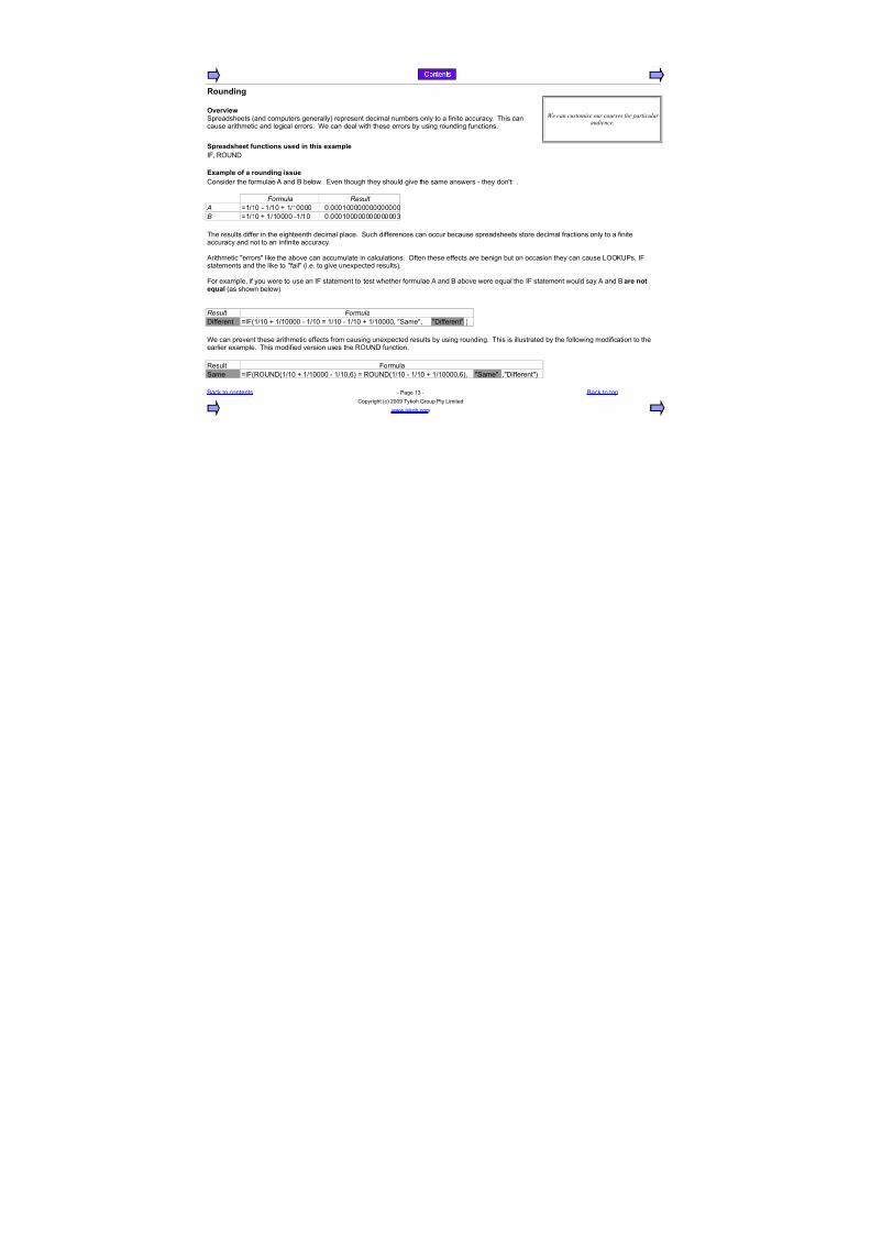
/ounding
Spreadsheet functions used in this example
I1 E2GF0
.xample of a rounding issue
Consider the formulae and & below. 7ven though they should give the same answers - they don't: .
4ormula 9esult
- O%%" - %%" Q %%"""" "."""%""""""""""""""
O%%" Q %%"""" -%%" "."""%"""""""""""""!
9esult 4ormula
0ifferent OI1%%" Q %%"""" - %%" O %%" - %%" Q %%"""" 4ame 0ifferent (
Eesult 1ormula
4ame OI1E2GF0%%" Q %%"""" - %%"( O E2GF0%%" - %%" Q %%""""( 4ame 0ifferent(
&ack to contents - $age %! - &ack to top
Copyright c( )""* Tykoh +roup $ty ,imited
www.tykoh.com
We can customise our courses for particularaudience
vervie!4preadsheets and computers generally( represent decimal numbers only to a finite accuracy. This can
cause arithmetic and logical errors. ;e can deal with these errors by using rounding functions.
The results differ in the eighteenth decimal place. 4uch differences can occur because spreadsheets store decimal fractions only to a finiteaccuracy and not to an infinite accuracy.
rithmetic errors like the above can accumulate in calculations. 2ften these effects are benign but on occasion they can cause ,22HG$s I1statements and the like to fail i.e. to give unexpected results(.
1or example if you were to use an I1 statement to test whether formulae and & above were e5ual the I1 statement would say and & are note0ual as shown below(.
;e can prevent these arithmetic effects from causing unexpected results by using rounding. This is illustrated by the following modification to theearlier example. This modified version uses the E2GF0 function.

7/18/2019 SpreadsheetGuide_1.02 (1) - copia
http://slidepdf.com/reader/full/spreadsheetguide102-1-copia 14/114
aluing & Scenarios & Attributing
vervie!
ttributing
4cenarios
Daluing
Spreadsheet functions used in this example
&4 F0 Conditional format C2GFT 0ata Table I1 6TC= 63 6IF 21147T 2E 4G
ttributing
$lease choose a scenario -M 3
4cenarios
4cenario Chosen &ase 4cenario % 4cenario )
nnual sales growth %"# %"# %"# 8#Current assets sales %"# %)# %)# %)#
This example is built on three levels. The lowest level is concerned with valuing an enterprisenumber of assumptions. The enterprise is valued on the basis of finding the present value of tavailable( cash flows it is expected to generate.
The middle level consists of a number of scenarios. 7ach scenario differs in its individual assenterprise value.
The highest level is concerned with attributing. =ere we look at how the enterprise value chachange in terms of the assumptions that differ between the scenarios.
&ase Curr assets sales 1ixed assets sales
"
@""
%"""
%@""
)"""
)@""
This is what makes e5uity value differ between base case
75uity value

7/18/2019 SpreadsheetGuide_1.02 (1) - copia
http://slidepdf.com/reader/full/spreadsheetguide102-1-copia 15/114
Current liabilities cost of good # # # #
Fet fixed assets sales @# A"# A"# A"#
Cost of goods sold sales @"# @@# @@# @@#
0epreciation rate %@# %@# %@# %*#
Interest rate on debt 8# 8# 8# 8#
Interest earned on cash balanc @# @# @# @#
Tax rate !!# !!# !@# !"#
0ividend payout ratio @@# @@# @@# @@#
0iscount rate %8# %8# %8# %8#
Terminal value multiple TD6( %) %) %% %"
2utput 75uity value %@! %9"@ %)A
7/18/2019 SpreadsheetGuide_1.02 (1) - copia
http://slidepdf.com/reader/full/spreadsheetguide102-1-copia 16/114
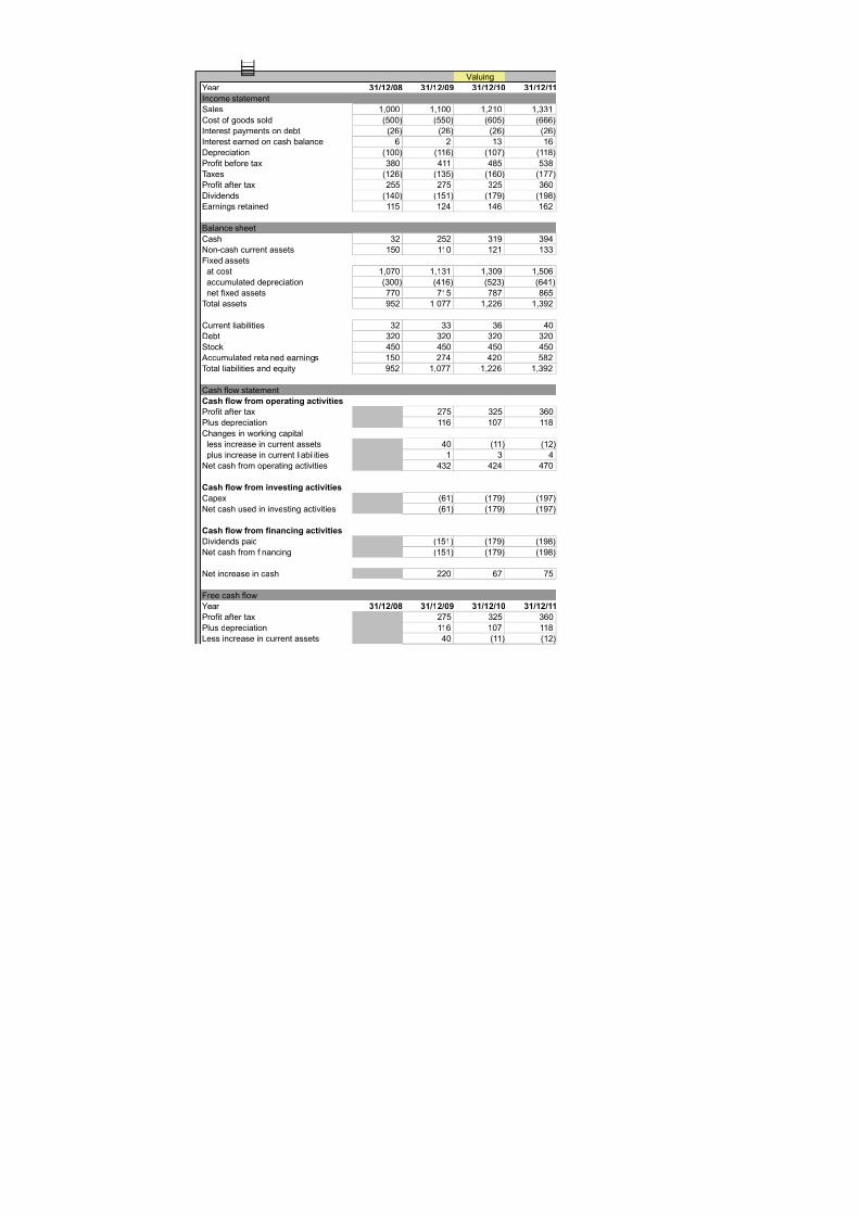
Daluing
>ear 31&12&*) 31&12&* 31&12&1* 31&12&11
Income statement
4ales %""" %%"" %)%" %!!%
Cost of goods sold @""( @@"( "@( (
Interest payments on debt )( )( )( )(
Interest earned on cash balance ) %! %
0epreciation %""( %%( %"A( %%8(
$rofit before tax !8" 9%% 98@ @!8
Taxes %)( %!@( %"( %AA(
$rofit after tax )@@ )A@ !)@ !"
0ividends %9"( %@%( %A*( %*8(
7arnings retained %%@ %)9 %9 %)
&alance sheet
Cash !) )@) !%* !*9
Fon-cash current assets %@" %%" %)% %!!1ixed assets
at cost %"A" %%!% %!"* %@"
accumulated depreciation !""( 9%( @)!( 9%(
net fixed assets AA" A%@ A8A 8@
Total assets *@) %"AA %)) %!*)
Current liabilities !) !! ! 9"
0ebt !)" !)" !)" !)"
4tock 9@" 9@" 9@" 9@"
ccumulated retained earnings %@" )A9 9)" @8)
Total liabilities and e5uity *@) %"AA %)) %!*)
Cash flow statement
Cash flo! from operating activities
$rofit after tax )A@ !)@ !"
$lus depreciation %% %"A %%8
Changes in working capital
less increase in current assets 9" %%( %)(
plus increase in current liabilities % ! 9
Fet cash from operating activities 9!) 9)9 9A"
Cash flo! from investing activities
Capex %( %A*( %*A(
Fet cash used in investing activities %( %A*( %*A(
Cash flo! from financing activities
0ividends paid %@%( %A*( %*8(
Fet cash from financing %@%( %A*( %*8(
Fet increase in cash ))" A A@
1ree cash flow
>ear 31&12&*) 31&12&* 31&12&1* 31&12&11
$rofit after tax )A@ !)@ !"
$lus depreciation %% %"A %%8,ess increase in current assets 9" %%( %)(

7/18/2019 SpreadsheetGuide_1.02 (1) - copia
http://slidepdf.com/reader/full/spreadsheetguide102-1-copia 17/114
$lus increase in current liabilities % ! 9
,ess increase in fixed assets at cost %( %A*( %*A(
$lus after tax interest on debt %A %A %A
,ess after tax interest on cash %( 8( %%(
1ree cash flow !8A )@9 )8"
Daluation
1ree cash flow 1C1( - !8A )@9 )8"
Terminal value multiple
Terminal value R 1C1 / multipleS - - - -
Total - !8A )@9 )8"
F$D )!A"
$lus cash !)
7nterprise value )9")
,ess debt !)"(
75uity value )"8)
&ack to contents - $age %9 -
Copyright c( )""* Tykoh +roup $ty ,imited
www.tykoh.com

7/18/2019 SpreadsheetGuide_1.02 (1) - copia
http://slidepdf.com/reader/full/spreadsheetguide102-1-copia 18/114
3F$D
4cenario ! 4cenario 9 4cenario @ 4cenario
1* %8# %8# %8#%"# %)# %)# %)#
Outsourcing of training functions ! one of the
services we offer based on ae free i.e.
umptions and each scenario generates an associated
nges between two scenarios. ;e explain that
C2+4 sales 4cenario !
and scenario !.

7/18/2019 SpreadsheetGuide_1.02 (1) - copia
http://slidepdf.com/reader/full/spreadsheetguide102-1-copia 19/114
# # #
@# A"# A"# A"#
@"# @@# @@# @@#
15 )"# )"# )"#
) 8# 8# 8#
5 @# @# @#
33 ))# )A# )#
55 @@# @@# @@#
1) %8# %8# %8#
12 %) %) %)
)"8) )""@ %A!* %A*)
7/18/2019 SpreadsheetGuide_1.02 (1) - copia
http://slidepdf.com/reader/full/spreadsheetguide102-1-copia 20/114
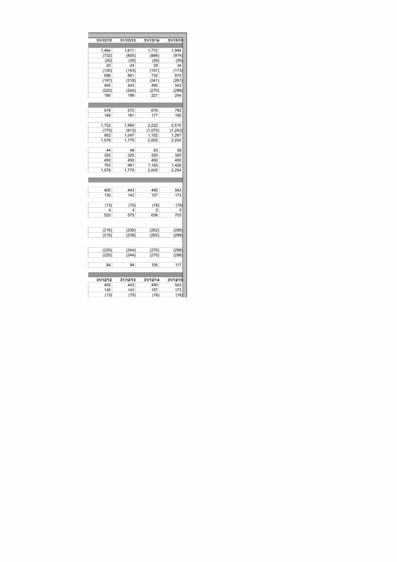
31&12&12 31&12&13 31&12&14 31&12&15
%99 %%% %AA) %*9*
A!)( 8"@( 88( *A9(
)( )( )( )(
)" )9 )* !9
%!"( %9!( %@A( %A!(
@* % A!) 8%"
%*A( )%8( )9%( )A(
9"" 99! 9*" @9!
))"( )99( )A"( )*8(
%8" %** ))% )99
9A8 @A) A A*!
%9 %% %AA %*@
%A)) %*" )))) )@%"
AA"( *%!( %"A"( %)9!(
*@) %"9A %%@) %)A
%@A %AA* )""@ ))@9
99 98 @! @8
!)" !)" !)" !)"
9@" 9@" 9@" 9@"
A) *% %%8) %9)
%@A %AA* )""@ ))@9
9"" 99! 9*" @9!
%!" %9! %@A %A!
%!( %@( %( %8(
9 9 @ @
@)" @A@ ! A"!
)%( )!8( ))( )88(
)%( )!8( ))( )88(
))"( )99( )A"( )*8(
))"( )99( )A"( )*8(
89 *9 %"@ %%A
31&12&12 31&12&13 31&12&14 31&12&15
9"" 99! 9*" @9!
%!" %9! %@A %A!%!( %@( %( %8(

7/18/2019 SpreadsheetGuide_1.02 (1) - copia
http://slidepdf.com/reader/full/spreadsheetguide102-1-copia 21/114
9 9 @ @
)%( )!8( ))( )88(
%A %A %A %A
%!( %( %*( )!(
!"8 !!8 !A) 9%"
!"8 !!8 !A) 9%"
%)
- 9*%9
!"8 !!8 !A) @!)9
&ack to top

7/18/2019 SpreadsheetGuide_1.02 (1) - copia
http://slidepdf.com/reader/full/spreadsheetguide102-1-copia 22/114
Scheduling events & cash flo!s
Spreadsheet functions used in this example F0 I1 I4F ,71T ,7F 6TC= 63 620 21147T 2E E2; D,22HG$
6essages
Fo messages
;vent 6cheduleas! $ength #rere)uisite % ) ! 9 @ A 8 * %" %% %) %! %9 %@ % %A %8 %* )" )% )) )! )9 )@ ) )A )8 )* !"
% C
& 9 0
C 9 LnoneM
0 9 7
7 ) 1
1 ) +
+ ) LnoneM
&ack to contents " - $age %@ - &ack to top
Copyright c( )""* Tykoh +roup $ty ,imited
www.tykoh.com
Our workshops review the finance principlesand assumptions underlying the main
spreadsheet financial functions
vervie! ctivities and events often proceed in a certain order. In spreadsheets the order of activities and eventscan be set in various ways: %( &y hard-coding them on a fixed timeline )( by using formulae to define
prere5uisites e.g. event & in row ) depends on event in row )@( !( in the way shown below. Theexample below implements a dynamic way of defining event dependencies and durations. In theexample below a task can proceed only when its prere5uisite has completed.
2ne challenge in managing a set of prere5uisites is to deal with the possibility of circularity. If you try to define a circular set of prere5uisites belowe.g. 's prere5uiste is & and &'s prere5uisite is ( you will see how this particular example deals with such a condition.

7/18/2019 SpreadsheetGuide_1.02 (1) - copia
http://slidepdf.com/reader/full/spreadsheetguide102-1-copia 23/114
Seasonalising
Spreadsheet functions used in this example
D7E+7 C=2247 Conditional format I1 4G6 T73T TE7F0
Choose data set )
4how seasonalised historic data
4how seasonalised future data
0ata sets
1 2 <
200/ =1 A*!) "" )""
=2 @!A A)* )A"=< !@! AA" ))
=> AA8) 88% %*9
200 =1 8"*% A) )%"
=2 @)8 A)@ %*)
=< AA" A %@
=> A8 8)) %@%
200 =1 8!A@ A"" %9
=2 *%9 89 %9
=< *!8 8!8 %9!
=> 8!*! 8! %!"
200 =1 8*98 A8! %!@
=2 8)88 88 %9%
=< A*" *" %9%
=> *A"* %"!) %@
&ack to contents - $age % - &ack to top
Copyright c( )""* Tykoh +roup $ty ,imited
www.tykoh.com
We specialise in presenting one and two
day finance / technical workshops
vervie!In seasonalising we determine patterns and trends in historic data. ;e can then back-fill the actual historicdata with seasonalised historic data to see how well the seasonalised data fits the historic. ;e can also roll-forward the seasonalised data to predict future values. n example is given below.
)"" )""A )""8 )""* )"%" )"%% )"%)
"
)""
9""
""
8""
%"""
%)""
0ata 4et )
c tua l h istori c 4easonal ised hi storic 4easonal ised futu re
7/18/2019 SpreadsheetGuide_1.02 (1) - copia
http://slidepdf.com/reader/full/spreadsheetguide102-1-copia 24/114
Column
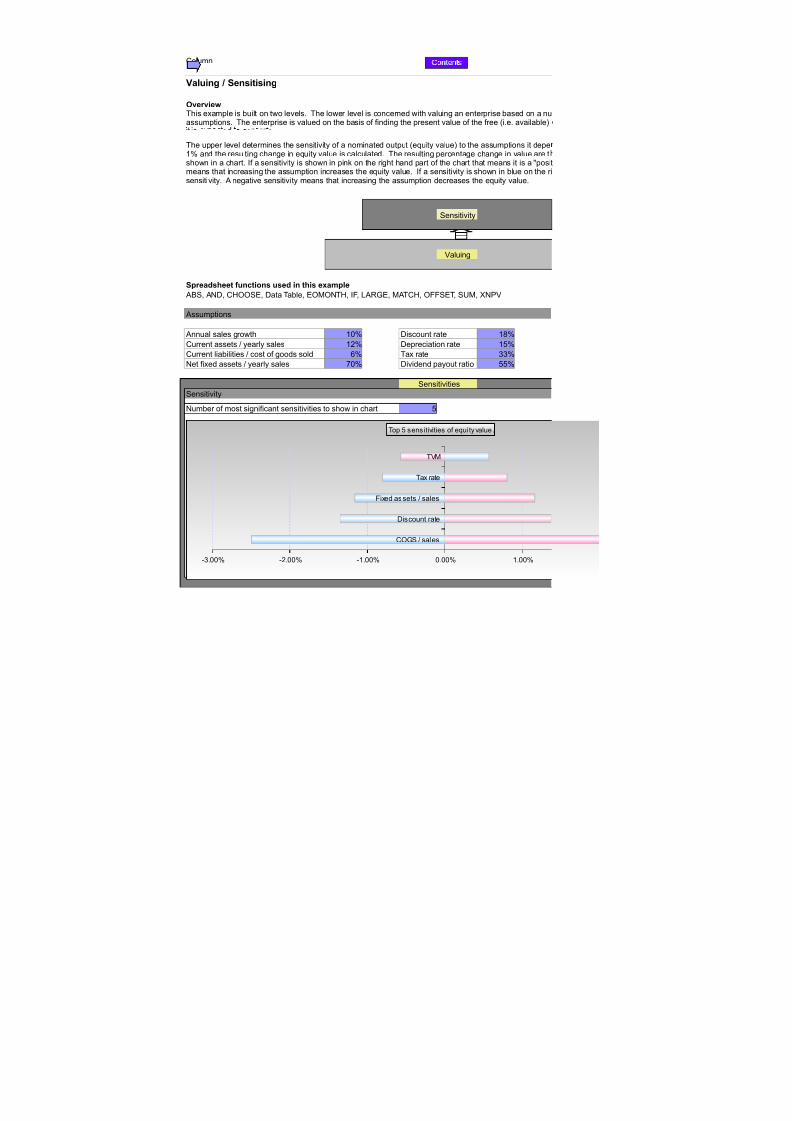
aluing & Sensitising
4ensitivity
Daluing
Spreadsheet functions used in this example
&4 F0 C=2247 0ata Table 7262FT= I1 ,E+7 6TC= 21147T 4G6 3F$D
ssumptions
nnual sales growth %"# 0iscount rate %8#
Current assets yearly sales %)# 0epreciation rate %@#Current liabilities cost of goods sold # Tax rate !!#
Fet fixed assets yearly sales A"# 0ividend payout ratio @@#
4ensitivities
4ensitivity
Fumber of most significant sensitivities to show in chart @
vervie!
This example is built on two levels. The lower level is concerned with valuing an enterprise based on a nuassumptions. The enterprise is valued on the basis of finding the present value of the free i.e. available(
The upper level determines the sensitivity of a nominated output e5uity value( to the assumptions it depe%# and the resulting change in e5uity value is calculated. The resulting percentage change in value are tshown in a chart. If a sensitivity is shown in pink on the right hand part of the chart that means it is a positmeans that increasing the assumption increases the e5uity value. If a sensitivity is shown in blue on the risensitivity. negative sensitivity means that increasing the assumption decreases the e5uity value.
C2+4 sales
0iscount rate
1ixed assets sales
Tax rate
TD6
-!.""# -).""# -%.""# ".""# %.""#
Top @ sens itivities of e5ui ty value.

7/18/2019 SpreadsheetGuide_1.02 (1) - copia
http://slidepdf.com/reader/full/spreadsheetguide102-1-copia 25/114
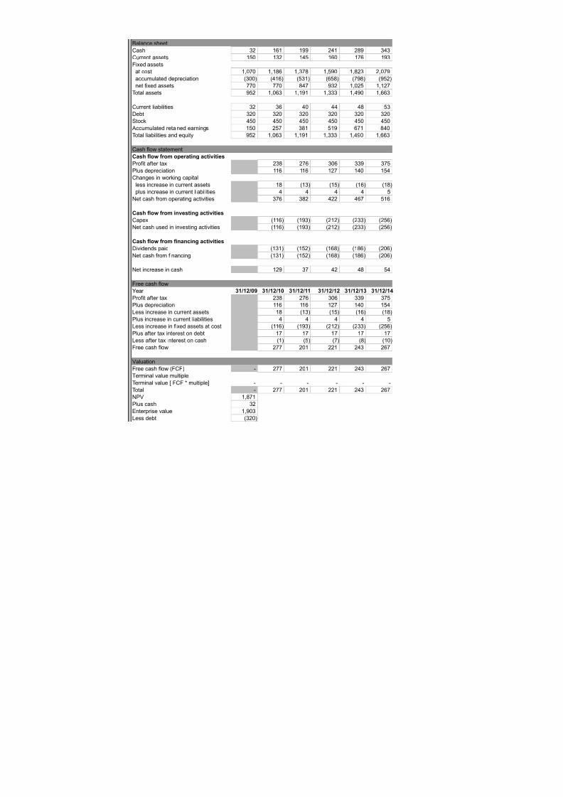
Daluing
Income statement
>ear 31&12&* 31&12&1* 31&12&11 31&12&12 31&12&13 31&12&14
4ales %""" %%"" %)%" %!!% %99 %%%
Cost of goods sold @@"( "@( ( A!)( 8"@( 88(
Interest payments on debt )( )( )( )( )( )(
Interest earned on cash balance ) 8 %" %) %9
0epreciation %""( %%( %%( %)A( %9"( %@9(
$rofit before tax !!" !@ 9%% 9@ @" @"
Taxes %"*( %%A( %!( %@%( %A( %8@(
$rofit after tax ))% )!8 )A !" !!* !A@
0ividends %))( %!%( %@)( %8( %8( )"(
7arnings retained %"" %"A %)9 %!8 %@) %*
7/18/2019 SpreadsheetGuide_1.02 (1) - copia
http://slidepdf.com/reader/full/spreadsheetguide102-1-copia 26/114
&alance sheet
Cash !) %% %** )9% )8* !9!
Current assets %@" %!) %9@ %" %A %*!
1ixed assets
at cost %"A" %%8 %!A8 %@*" %8)! )"A*
accumulated depreciation !""( 9%( @!%( @8( A*8( *@)(
net fixed assets AA" AA" 89A *!) %")@ %%)A
Total assets *@) %"! %%*% %!!! %9*" %!
Current liabilities !) ! 9" 99 98 @!
0ebt !)" !)" !)" !)" !)" !)"
4tock 9@" 9@" 9@" 9@" 9@" 9@"
ccumulated retained earnings %@" )@A !8% @%* A% 89"
Total liabilities and e5uity *@) %"! %%*% %!!! %9*" %!
Cash flow statement
Cash flo! from operating activities
$rofit after tax )!8 )A !" !!* !A@$lus depreciation %% %% %)A %9" %@9
Changes in working capital
less increase in current assets %8 %!( %@( %( %8(
plus increase in current liabilities 9 9 9 9 @
Fet cash from operating activities !A !8) 9)) 9A @%
Cash flo! from investing activities
Capex %%( %*!( )%)( )!!( )@(
Fet cash used in investing activities %%( %*!( )%)( )!!( )@(
Cash flo! from financing activities
0ividends paid %!%( %@)( %8( %8( )"(Fet cash from financing %!%( %@)( %8( %8( )"(
Fet increase in cash %)* !A 9) 98 @9
1ree cash flow
>ear 31&12&* 31&12&1* 31&12&11 31&12&12 31&12&13 31&12&14
$rofit after tax )!8 )A !" !!* !A@
$lus depreciation %% %% %)A %9" %@9
,ess increase in current assets %8 %!( %@( %( %8(
$lus increase in current liabilities 9 9 9 9 @
,ess increase in fixed assets at cost %%( %*!( )%)( )!!( )@(
$lus after tax interest on debt %A %A %A %A %A
,ess after tax interest on cash %( @( A( 8( %"(
1ree cash flow )AA )"% ))% )9! )A
Daluation
1ree cash flow 1C1( - )AA )"% ))% )9! )A
Terminal value multiple
Terminal value R 1C1 / multipleS - - - - - -
Total - )AA )"% ))% )9! )A
F$D %8A%
$lus cash !)
7nterprise value %*"!,ess debt !)"(

7/18/2019 SpreadsheetGuide_1.02 (1) - copia
http://slidepdf.com/reader/full/spreadsheetguide102-1-copia 27/114
75uity value %@8!
&ack to contents - $age %A -
Copyright c( )""* Tykoh +roup $ty ,imited
www.tykoh.com

7/18/2019 SpreadsheetGuide_1.02 (1) - copia
http://slidepdf.com/reader/full/spreadsheetguide102-1-copia 28/114
Interest rate on debt 8#
Interest earned on cash @#Cost of goods sold sales @@#
Terminal value multiple TD6( %)
'eedback from our 'inancial (odelling course) %*nderstanding the
complex Excel tips was verybeneficial%
mber ofcash flows
ds on. 7ach assumption is changed byen ranked in order of significance andive sensitivity. positive sensitivityght hand side it represents a negative
).""# !.""#

7/18/2019 SpreadsheetGuide_1.02 (1) - copia
http://slidepdf.com/reader/full/spreadsheetguide102-1-copia 29/114
31&12&15 31&12&1 31&12&1 31&12&1)
%AA) %*9* )%99 )!@8
*A9( %"A)( %%A*( %)*A(
)( )( )( )(
%A )" )! )A
%*( %8( )"@( ))@(
)" 8@ A@8 8!8
)"9( ))( )@"( )A(
9%@ 9@* @"8 @%
))8( )@!( )A*( !"*(
%8A )"A ))* )@!

7/18/2019 SpreadsheetGuide_1.02 (1) - copia
http://slidepdf.com/reader/full/spreadsheetguide102-1-copia 30/114
9"! 9A" @9@ )*
)%! )!9 )@A )8!
)!% )A% !"%) !!8A
%%)%( %!"A( %@%%( %A!(
%)9" %!9 %@"% %@%
%8@@ )"8 )!"! )@)
@8 9 A% A8
!)" !)" !)" !)"
9@" 9@" 9@" 9@"
%")A %)!! %9) %A%@
%8@@ )"8 )!"! )@)
9%@ 9@* @"8 @%%* %8 )"@ ))@
%*( )%( )!( )(
@ A
@A" !" *@ A8
)8)( !%"( !9%( !A@(
)8)( !%"( !9%( !A@(
))8( )@!( )A*( !"*())8( )@!( )A*( !"*(
" A A@ 89
31&12&15 31&12&1 31&12&1 31&12&1)
9%@ 9@* @"8 @%
%* %8 )"@ ))@
%*( )%( )!( )(
@ A
)8)( !%"( !9%( !A@(
%A %A %A %A
%%( %!( %( %8(
)*9 !)! !@ !*%
)*9 !)! !@ !*%
%)
- - - 9*A
)*9 !)! !@ @"88

7/18/2019 SpreadsheetGuide_1.02 (1) - copia
http://slidepdf.com/reader/full/spreadsheetguide102-1-copia 31/114
&ack to top

7/18/2019 SpreadsheetGuide_1.02 (1) - copia
http://slidepdf.com/reader/full/spreadsheetguide102-1-copia 32/114
aluing contingencies
Spreadsheet functions used in this example
C=2247 0ata Table 73$ I1 ,F 6TC= 63 F2E640I4T 4BET 4G6
-sset #rice %""
7ption type
Call european( %"" ".% % ?olatility )"#
Call european( A8 "."@ -) @ield %.@#
Call asset-or-nothing( 8" ".% % 9is! free rate @.@#
Total
% %
)
!
"
&ack to contents - $age %8 -
Copyright c( )""* Tykoh +roup $ty ,imi ted
Our financial modelling course shows theessential building blocks of efficient and well!
presented financial models
vervie!To put a value on contingencies we need to take probabilities into account e.g. how likely is thecontingency to occur(. n example of a contingency is an option position. ;hether the option pays off iscontingent on the performance of an underlying asset. 1ortunately &lack 4choles developed a formulafor pricing some options that saves us many difficult probability calculations. The &lack 4choles formula isused in the example below.
call option gives you the right - but not the obligation - to buy something at a future date at a price that is set today. The price at which thepurchase will be done if it is done( is called the exercise price. put option gives you the right to sell something at a future date at a price that isset today. gain the price at which the sale will be done if it is done( is the exercise price.
;xercise price
5aturity %inyears'
#osition[num,er held
A %sold'] 6ho( on
chart
&ack to top
www.tykoh.com
" A" 8" *" %"" %%" %)" %!" %9"
-%@"
-%""
-@"
"
@"
%""
%@"
)""
Dalue of option portfolio as f unction of asset price
2pt ion % O Cal l eu ropean( 2pt ion ) O Cal l european( 2p tion ! O Cal l asset -or -nothing (
Lnot shownM

7/18/2019 SpreadsheetGuide_1.02 (1) - copia
http://slidepdf.com/reader/full/spreadsheetguide102-1-copia 33/114
isual ,asic
Disual &asic is part of most 6icrosoft 2ffice products and it gives you the power to:
- utomate routine work and save the time and trouble of doing the same thing over and over - Increase work efficiency by making shortcuts for common tasks
-
CustomiNe 6icrosoft 2ffice products to your needs by extending or changing those products' functionality
- Integrate workflows across 6icrosoft 2ffice applications
- Increase the wow-factor of your developed applications
&ack to contents KF67< &ack to top
Copyright c( )""* Tykoh +roup $ty ,imitedwww.tykoh.com
+eview how financial statements can bemodelled in spreadsheets ! attend one of our
workshops
Disual &asic is not used in any of the examples in this spreadsheet. =owever if you are interested in some examples of Disual &asic's applicationor wish to enrol on a Disual &asic workshop please visit the following web site:
Disual &asic ;orkshop

7/18/2019 SpreadsheetGuide_1.02 (1) - copia
http://slidepdf.com/reader/full/spreadsheetguide102-1-copia 34/114
Cross reference of functions used in the examples & Summar'
- The examples use only a small number of functions. The average number of functions used in each example is approximately 8.
Cross reference
;xample n u m f u n c t i o n s u s e d
- r r
a y s
C 2
0 7
C o n d i t i o n a l f o r m a t
0 a t a T a b l e
7 2
6 2 F T =
7 3
$
I F T , F 6 I F D 7 E 4 7
6 6
G , T
6 2
0
F 2
E 6 4 0 I 4 T
E 2
G F 0
E 2
;
4 B
E T
T 7
3 T
T E
7 F 0
3 F
$ D
ggregating o o o o o o
veraging @ o o o o o
Charting o o o o o o
=ighlighting A o o o o o o o
1iltering 8 o o o o o o o o
Interpolating 8 o o o o o o o o
,ooking up 8 o o o o o o o o
$rioritising ! o o o
Eanking * o o o o o o o o o
Eounding ) o o
4cenarios %! o o o o o o o o o o o o o
4cheduling %) o o o o o o o o o o o o
4easonalising A o o o o o o o
4ensitivities %% o o o o o o o o o o oInterest rates 8 o o o o o o o o
Daluing contingency %" o o o o o o o o o o
&ack to contents - $age )" - &ack to top
Copyright c( )""* Tykoh +roup $ty ,imited
www.tykoh.com
We use high!tech modes of teachingand course content delivery
vervie!&elow is a cross reference showing the spreadsheet functions and features used in each of the examples in this
chapter 4everal interesting observations can be made from the information in the cross reference:
- The total number of functions used in all the examples is 9". That is about %)# of the functions available. In other words seven of every eightfunctions available were not used in any of the examples.
4unctions and features used %4unctions in ,lue are descri,ed in Chapter <'
- &
4
- F
0
- D 7 E - + 7
C =
2 2 4 7
C 2
G F T
C 2
G F T I 1
I 1 I 4 F
-
, - E + 7
, 7 1 T
, 7 F
, 2
2 H G $
6 -
T C =
6 -
3
6 I 0 6 I F
2 1
1 4 7 T
2 E E I +
= T
4 G
6
4 G
6 $ E 2 0 G C T
D , 2 2 H G $
Summar'7ven though some of the examples in this spreadsheet are complex we can see that they are built from a small number of functions. 4o wheredoes the complexity and power and usefulness of the examples come from< It comes from the arrangement of individually simple functions into acomplex whole. This points to the importance and benefits of design - being able to build something complex from things that are simple.
nother lesson from the examples is the benefit of focusing ones' learning on a subset of spreadsheet functions: In these examples approximately9" functions out of !)" are particularly useful to know about. The other )8" - odd might be applicable only infre5uently.

7/18/2019 SpreadsheetGuide_1.02 (1) - copia
http://slidepdf.com/reader/full/spreadsheetguide102-1-copia 35/114
Chapter 2 - Functions
#unctions;hat do we mean by the word function< function is part or all( of a spreadsheet formula. Consider th
6-2 7 S8M9A1:,2; < C2
6S8M91= A1:#4= 2 < 3= ,2;
This function has four arguments. The first is % the second is %:19 the third is ) /! and the fourth is &).
A,S function
& C 0 7 1 + =
%
) &rokerage fee R#S )#!
This chapter contains a description of some spreadsheet functions. s with the rest of this book - some s
interactive. 6ost if not all of the functions described in this chapter are used in the application examples i).
In the formula above S8M is a function. >ou can tell it's a function because it consists of letters of the alpbracket. nytime you see letters of the alphabet followed by a open bracket - you know you're looking at
;hat does a function do< That depends on the function. 0ifferent functions do different things. The 4Gfunction averages numbers the C=2247 function lets you choose between numbers and so on.
If you're using the 4G6 function to sum numbers how does the function know which numbers you wantdirectly Ras in O4G6% ) @(S or by giving it cell references that contain the numbers Ras in O4G6% !
4o to use a function you almost always pass it information for it to work with. That information is containe
In the 4G6 example above A1:,2 describes the numbers we want to sum. 4o A1:,2 is the argument offunction has a single argument. If a function has more than one argument then they are separated by co
Fow that we've introduced the concept of functions and arguments we'll describe some of the most usefulfunctions are ordered alphabetically.
The &4 function returns the absolute value of its argument. The absolute value of a number is obtainedThe argument to the &4 must be a single number or cell reference. If the argument is positive then thenumber is negative then the positive version of that number is returned i.e. the sign is removed(.
;here would you use an &4 function< ;e'll look at an example to do with calculating buying and sellinwill calculate a brokerage fee to pay on a sale of P!""""". ;e will use a convention whereby cash comiis negative. &ecause we are selling something that will be cash coming in and so we'll represent that as
The brokerage calculation is in cell 0. The brokerage is calculated by multiplying the brokerage percentpurchase. &oth the percentage fee and the sale amount are positive numbers. &ut since the brokerage fnegative. 4o there is a negative sign at the front of the formula in 0.

7/18/2019 SpreadsheetGuide_1.02 (1) - copia
http://slidepdf.com/reader/full/spreadsheetguide102-1-copia 36/114
9 4ale purchase( RP"""'sS !""
@
&rokerage RP"""'sS -
A
Continuing with our example - ;e find the brokerage fee to be P""" and it is a negative number.
& C 0 7 1 + =
%
) &rokerage fee R#S )#
!9 4ale purchase( RP"""'sS -9""
@
&rokerage RP"""'sS 8
A
L- O-0)/09
[Cell ;/ is a comment. +t sho(s the formula in the cell to its left. 6o ,y loo!ing at cell ;/ (e can tell thatD2 and D> cells in the ;/ formula are colour coded. he cells ;/ refers to are also colour coded (ith colD> has a ,lue ,order. he colour coding ma!es it easy to see (hich cells in the spreadsheet a formula r
4uppose we now use our spreadsheet to calculate the brokerage on a purchase of P9""""". The numba cash outlay.
L- O-0)/09
7/18/2019 SpreadsheetGuide_1.02 (1) - copia
http://slidepdf.com/reader/full/spreadsheetguide102-1-copia 37/114
& C 0 7 1 + =
%
) &rokerage fee R#S )# )#
!
9 4ale purchase( RP"""'sS !"" -9""
@
&rokerage RP"""'sS - -8
A
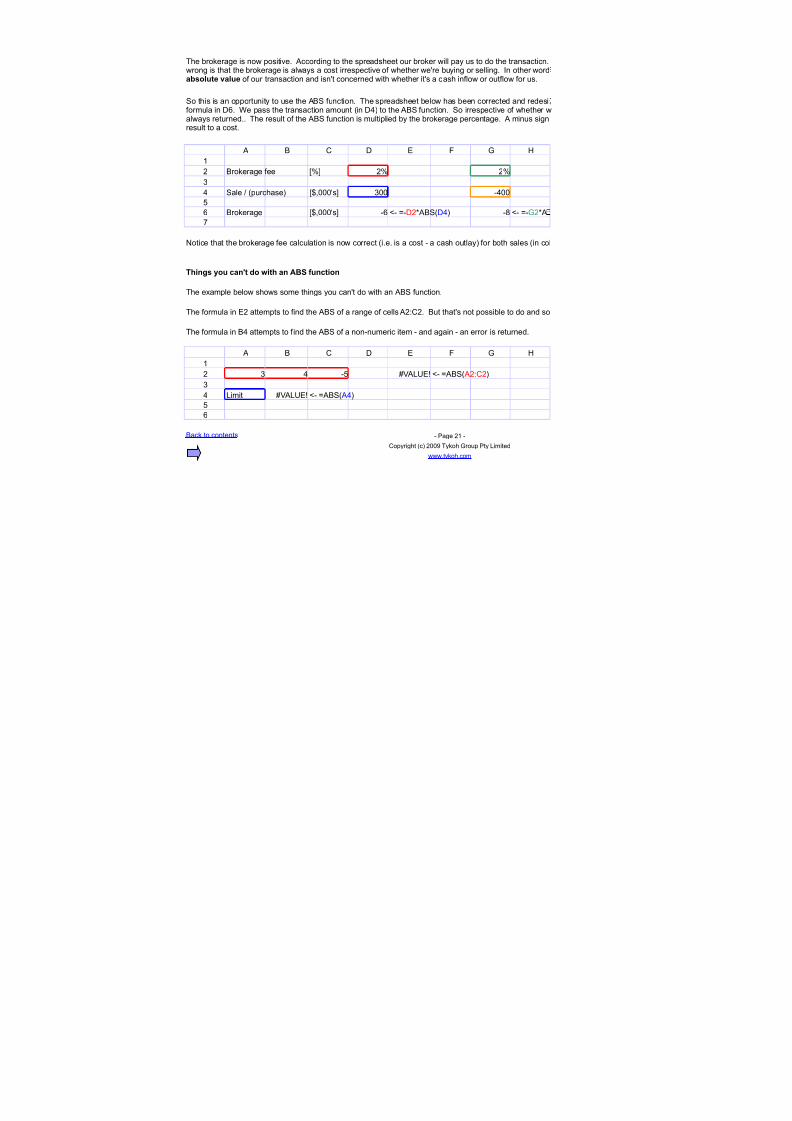
Fotice that the brokerage fee calculation is now correct i.e. is a cost - a cash outlay( for both sales in col
?hings 'ou can@t do !ith an A,S function
The example below shows some things you can't do with an &4 function.
The formula in 7) attempts to find the &4 of a range of cells ):C). &ut that's not possible to do and so
The formula in &9 attempts to find the &4 of a non-numeric item - and again - an error is returned.
& C 0 7 1 + =
%
) ! 9 -@ KD,G7?
!
9 ,imit KD,G7?
@
&ack to contents - $age )% -
Copyright c( )""* Tykoh +roup $ty ,imited
www.tykoh.com
The brokerage is now positive. ccording to the spreadsheet our broker will pay us to do the transaction.wrong is that the brokerage is always a cost irrespective of whether we're buying or selling. In other wordabsolute value of our transaction and isn't concerned with whether it's a cash inflow or outflow for us.
4o this is an opportunity to use the &4 function. The spreadsheet below has been corrected and redesiformula in 0. ;e pass the transaction amount in 09( to the &4 function. 4o irrespective of whether walways returned.. The result of the &4 function is multiplied by the brokerage percentage. minus signresult to a cost.
L- O-0)/&409( L- O-+)/
L- O&4 ):C)(
L- O&4 9(
7/18/2019 SpreadsheetGuide_1.02 (1) - copia
http://slidepdf.com/reader/full/spreadsheetguide102-1-copia 38/114
formula below.
.
'eedback from our ,preadsheet skills
course) %Excellent knowledge and clearcommunication from the presenter%
ections are
n Chapter
habet immediately followed by an opena function.
function adds numbers the D7E+7
to add< >ou tell it by giving it the numbers &:+A(S.
d in a list of parameters or arguments>
the 4G6 function. In this example the 4G6mas. Consider the following example.
l spreadsheet functions. In this chapter the
by removing any minus sign it might have.umber is returned unchanged. If the
commissions. In the illustration below weng in is a positive number and cash going out
positive number.
ge fee by the amount of the sale ore is a cash outgoing we need to make that
'eedback from our 'inancial (odelling
course) %*nderstanding the complex Excel tips was very beneficial%

7/18/2019 SpreadsheetGuide_1.02 (1) - copia
http://slidepdf.com/reader/full/spreadsheetguide102-1-copia 39/114
the formula in D/ is BD2 * D>. @oull notice theured ,orders: Cell D2 has a red ,order andfers to.]
er in 09 is now negative since a purchase is
'eedback from our Visual Basic course)%-he material covered will be very useful
at work as the . and workbook provided%
7/18/2019 SpreadsheetGuide_1.02 (1) - copia
http://slidepdf.com/reader/full/spreadsheetguide102-1-copia 40/114
I
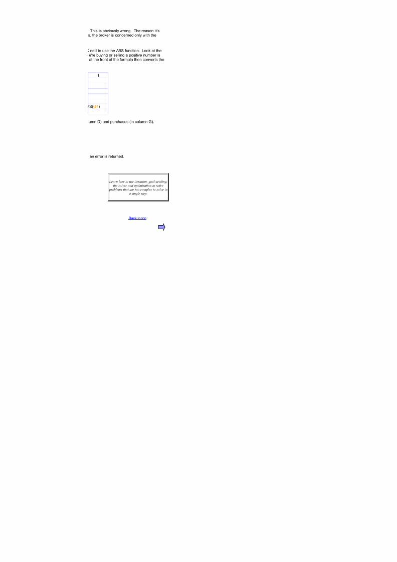
umn 0( and purchases in column +(.
an error is returned.
&ack to top
This is obviously wrong. The reason it'ss the broker is concerned only with the
ned to use the &4 function. ,ook at thee're buying or selling a positive number isat the front of the formula then converts the
4+9(
"earn how to use iteration$ goal!seeking$the solver and optimisation to solve
problems that are too complex to solve ina single step

7/18/2019 SpreadsheetGuide_1.02 (1) - copia
http://slidepdf.com/reader/full/spreadsheetguide102-1-copia 41/114
A- function
& C 0 7 1 + =
%
) % L- OF0TEG7TEG7(
!
9 " L- OF0TEG71,47(
@
" L- OF01,471,47(
A
In this section and throughout the rest of this guide we use a colouring convention to mark those cells t
Cells you can change are shown with a blue background and white text. 4uch cells will look like:
nother colouring convention is used to show output cells. These are cells that will change when you
cells. 4uch cells have a black background and white text and look like this: "
& C 0 7 1 + =
% % % "
)
!
9 "
@
(ogical tests and conditions
& C 0 7 1 + =
% % @ A
)
! " @ A
9
& C 0 7 1 + =
% % ,ondon 4ingapore
)
The F0 function accepts a number of TEG7 and 1,47 parameters and returns TEG7 if all of the pa
are TEG7. It returns 1,47 otherwise.
1ollowing is an interactive example. >ou can set % C% and 7% to TEG7 or 1,47. The F0 function
7% are all TEG7.
L- OF0 %C%7%(
In the example above the arguments to the F0 function are explicitly TEG7 or 1,47. In practice theresult of logical tests or conditions - as illustrated in the example below.
L- O7%L+%
L- O7!M+!
Cell % contains the logical test 7%L+%. ,ogical tests involve comparing two 5uantities and determininone is less than the other one is greater than or e5ual to the other and so on. The result of the logicalTEG7 because 7% @( is less than +% A(. The test in ! is 1,47 because 7! is not greater than +!.
The items being compared in logical tests can be text strings(. This is illustrated in the following exatheir alphabetical order. 4o for example ,ondon is less than 4ingapore.
L- O7%L+%

7/18/2019 SpreadsheetGuide_1.02 (1) - copia
http://slidepdf.com/reader/full/spreadsheetguide102-1-copia 42/114
! % 0ept-= 0ept-B
9
@ " Few >ork 9@
A
& C 0 7 1 + =
% Fum % Fum )
) % ! A
!
9 " ! *
@
" * !
A
& C 0 7 1 + =
% )""8 )""*
) &udget %@ %8
!
9 ctual %9 %A
@ ;ithin budget: %
A
L- O7!L+!
L- O7@L+@
It doesn't really make sense to compare numbers with strings and it's difficult to imagine why anyone willustrated in the formula in @ above.
In the illustration below we use an F0 function to determine whether each number in the + column iscolumns. 2nly on row ) are both tests in the F0 satisfied and so only on row ) is + between 7 and I.
L- OF07)L+)+)LI)(
L- OF079L+9+9LI9(
L- OF07L++LI(
The following interactive example relates to budgeting. ;e want to know whether the actual figures incan change the actual figures and observe whether the ;ithin budget result is as you'd expect.
L- OF0&9LO&)C9LOC)(
7/18/2019 SpreadsheetGuide_1.02 (1) - copia
http://slidepdf.com/reader/full/spreadsheetguide102-1-copia 43/114
& C 0 7 1 + =
% )""8 )""*
) &udget %@ %8
!
9 ctual %9 %*
@
A
8 ;ithin budget: outside
*
/ function
& C 0 7 1 + =
% >ear +rowth ;ithin budget 1lag
) %**A @# yes
! %**8 !# yes
9 %*** %"# yes
@ )""" -%)# yes x )""% @# yes
A )"") !# yes
8 )""! @# no x
* )""9 A# yes
%" )""@ -!# no x
%% )"" )# yes @#
%) )""A # yes -!#
%! )""8 %# yes
%9 )""* -)# yes x
%@
&ack to contents - $age )) -
Copyright c( )""* Tykoh +roup $ty ,imited
www.tykoh.com
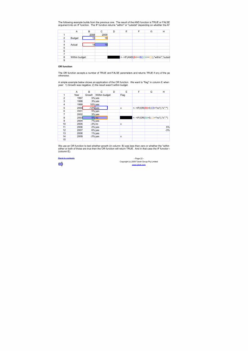
The following example builds from the previous one. The result of the F0 function is TEG7 or 1,47argument into an I1 function. The I1 function returns within or outside depending on whether the
L- OI1F0&9LO&)C9LOC)(withinoutsid
The 2E function accepts a number of TEG7 and 1,47 parameters and returns TEG7 if any of the paotherwise.
simple example below shows an application of the 2E function. ;e want to flag in column 7 whenyear: %( +rowth was negative )( the result wasn't within budget.
L- OI12E&@L"C@Ono(x(
L- OI12E&8L"C8Ono(x(
;e use an 2E function to test whether growth in column &( was less than Nero or whether the withineither or both of those are true then the 2E function will return TEG7. nd in that case the I1 functioncolumn 7(.

7/18/2019 SpreadsheetGuide_1.02 (1) - copia
http://slidepdf.com/reader/full/spreadsheetguide102-1-copia 44/114
at you can change.
.!"#
change one of the blue background
Our Visual Basic course shows how to
increase work efficiency by making shortcuts for common tasks
rameters
in 9 will return TEG7 only when % C% and
Our modelling and spreadsheet skillscourses cover both core and extended
spreadsheet and finance topics
TEG7 and 1,47 arguments will be the
whether they are e5ual to each other ortest is TEG7 or 1,47. The test in % is
ple. 4trings are compared on the basis of
'eedback from our Visual Basic course)
%-he material covered will be very usefulat work as the . and workbook

7/18/2019 SpreadsheetGuide_1.02 (1) - copia
http://slidepdf.com/reader/full/spreadsheetguide102-1-copia 45/114
I
Fum !
*
A
A
provided%
uld want to do this - but it can be done - as
between the numbers in the 7 and I
oth )""8 and )""* were within budget. >ou
012V gives a different answer if cellsare blank than when they contain 3ero !these and other %traps% are explained in
our workshops
7/18/2019 SpreadsheetGuide_1.02 (1) - copia
http://slidepdf.com/reader/full/spreadsheetguide102-1-copia 46/114
I
&ack to top
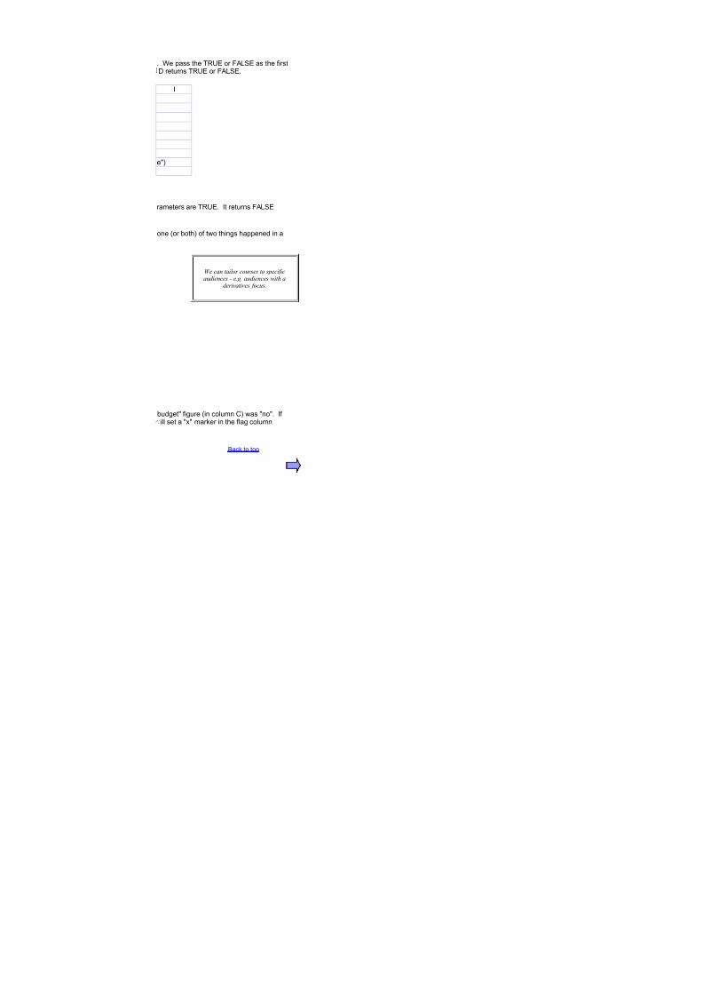
. ;e pass the TEG7 or 1,47 as the first0 returns TEG7 or 1,47.
e(
rameters are TEG7. It returns 1,47
one or both( of two things happened in a
We can tailor courses to specificaudiences ! eg audiences with a
derivatives focus
budget figure in column C( was no. Ifill set a x marker in the flag column

7/18/2019 SpreadsheetGuide_1.02 (1) - copia
http://slidepdf.com/reader/full/spreadsheetguide102-1-copia 47/114
A./AB. function
& C 0 7 1 + =
% % ! )
)
! % ! )9
@ % " ! %.!!!!!!!
A K0ID"?
&ack to contents - $age )! - &ack to top
Copyright c( )""* Tykoh +roup $ty ,imited
www.tykoh.com
2articipants on our courses have theopportunity to do on!line pre and post!
course self!evaluations
The D7E+7 function returns the average of one or more arguments. The arguments can contain individualnumbers or cells or groups of cells. 4ome usages of the average function are shown below.
In cell 0% we use the D7E+7 function to find the average of two individual cells: % contains % and C% contains! and so the average is ).
In cell 0! we use D7E+7 to find the average of a block of cells: !:C!. Fote that cell &! is empty and that D7E+7 is ignoring that cell. 4othe calcuation it is making is this: O% Q !() O ). If D7E+7 had included &! in its calculation it would have arrived at a different result: O% Q " Q!(! O %.!!!.
In cell 0@ D7E+7 is working with a similar set of cells as it did on row !. =owever in this example the middle cell has " explicitly in it instead ofbeing empty. ;e can see that this changes the result of the average from ) to %.!!!!
L- OD7E+7 %C%(
Outsourcing of training functions ! oneof the services we offerL- OD7E+7 !:C!(
L- OD7E+7 @:C@(
L- OD7E+7 A:CA(
In cell 0A D7E+7's argument is a range that contains no numbers at all. In this case D7E+7's calculation is this: O"". >ou cannot divide byNero and so the error occurs.
R1or an example of the D7E+7 function used with the 21147T function click hereS
R1or an example of an application that uses D7E+7 click hereS
7/18/2019 SpreadsheetGuide_1.02 (1) - copia
http://slidepdf.com/reader/full/spreadsheetguide102-1-copia 48/114
C"S. function
In the following example the C=2247 function's first argument is %. 4o the first following argument i.e. the second - %( is returned.
& C 0 7 1 + =
% 9@ 8) %A
)
! 9@
9
In the following example the C=2247 function's first argument is ). 4o the second following argument i.e. the third - C%( is returned.
& C 0 7 1 + =
% 9@ 8) %A
)
! 8)
9
Choosing a scenario
& C 0 7 1 + =
% 4cenario: % - Feutral ) - 2ptimistic ! - $essimistic
) 9@ 8) %A
!
9 ) Eesult: 8)
@
& C 0 7 1 + =% 9@ 8) %A
)
! 7rr:@")
9
& C 0 7 1 + =
% 9@ 8) %A
)! 7rr:@")
9
& C 0 7 1 + =
% % ) !
Our Visual Basic course shows how toincrease the %wow!factor% of your
developed applications
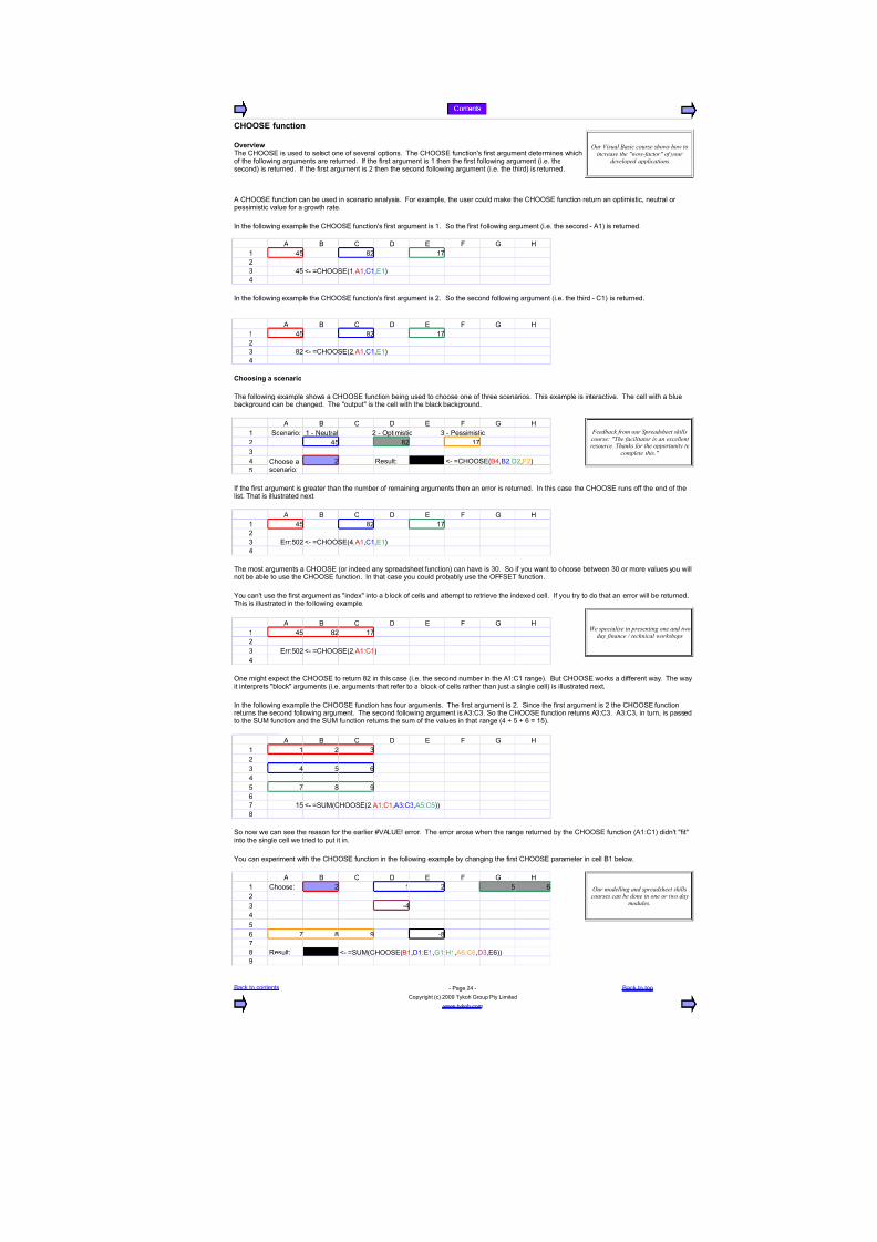
vervie!The C=2247 is used to select one of several options. The C=2247 function's first argument determines whichof the following arguments are returned. If the first argument is % then the first following argument i.e. thesecond( is returned. If the first argument is ) then the second following argument i.e. the third( is returned.
C=2247 function can be used in scenario analysis. 1or example the user could make the C=2247 function return an optimistic neutral orpessimistic value for a growth rate.
L- OC=2247% %C%7%(
L- OC=2247) %C%7%(
The following example shows a C=2247 function being used to choose one of three scenarios. This example is interactive. The cell with a bluebackground can be changed. The output is the cell with the black background.
'eedback from our ,preadsheet skillscourse) %-he facilitator is an excellentresource -hanks for the opportunity to
complete this%
Choose ascenario:
L- OC=2247&9&)0)1)(
If the first argument is greater than the number of remaining arguments then an error is returned. In this case the C=2247 runs off the end of thelist. That is illustrated next.
L- OC=22479 %C%7%(
The most arguments a C=2247 or indeed any spreadsheet function( can have is !". 4o if you want to choose between !" or more values you willnot be able to use the C=2247 function. In that case you could probably use the 21147T function.
>ou can't use the first argument as index into a block of cells and attempt to retrieve the indexed cell. If you try to do that an error will be returned.This is illustrated in the following example.
We specialise in presenting one and twoday finance / technical workshops
L- OC=2247) %:C%(
2ne might expect the C=2247 to return 8) in this case i.e. the second number in the %:C% range(. &ut C=2247 works a different way. The wayit interprets block arguments i.e. arguments that refer to a block of cells rather than ust a single cell( is illustrated next.
In the following example the C=2247 function has four arguments. The first argument is ). 4ince the first argument is ) the C=2247 functionreturns the second following argument. The second following argument is !:C!. 4o the C=2247 function returns !:C!. !:C! in turn is passedto the 4G6 function and the 4G6 function returns the sum of the values in that range 9 Q @ Q O %@(.
7/18/2019 SpreadsheetGuide_1.02 (1) - copia
http://slidepdf.com/reader/full/spreadsheetguide102-1-copia 49/114
C8? function
& C 0 7 1 + =
%
) ! K0ID"?
! above 9
9
@ )
& C 0 7 1 + =%
) ! 9 @
! A 8
9 * %" %%
@ %) %! %9
A ok
8
& C 0 7 1 + =
%
) ! 9 @
! A 8
9 * %" %%
@ %) %! %9
A 7rror
8
&ack to contents - $age )@ - &ack to top
Copyright c( )""* Tykoh +roup $ty ,imited
www.tykoh.com
"earn the ob#ectives$ principles andmethods of financial modelling byattending our financial modelling
workshop
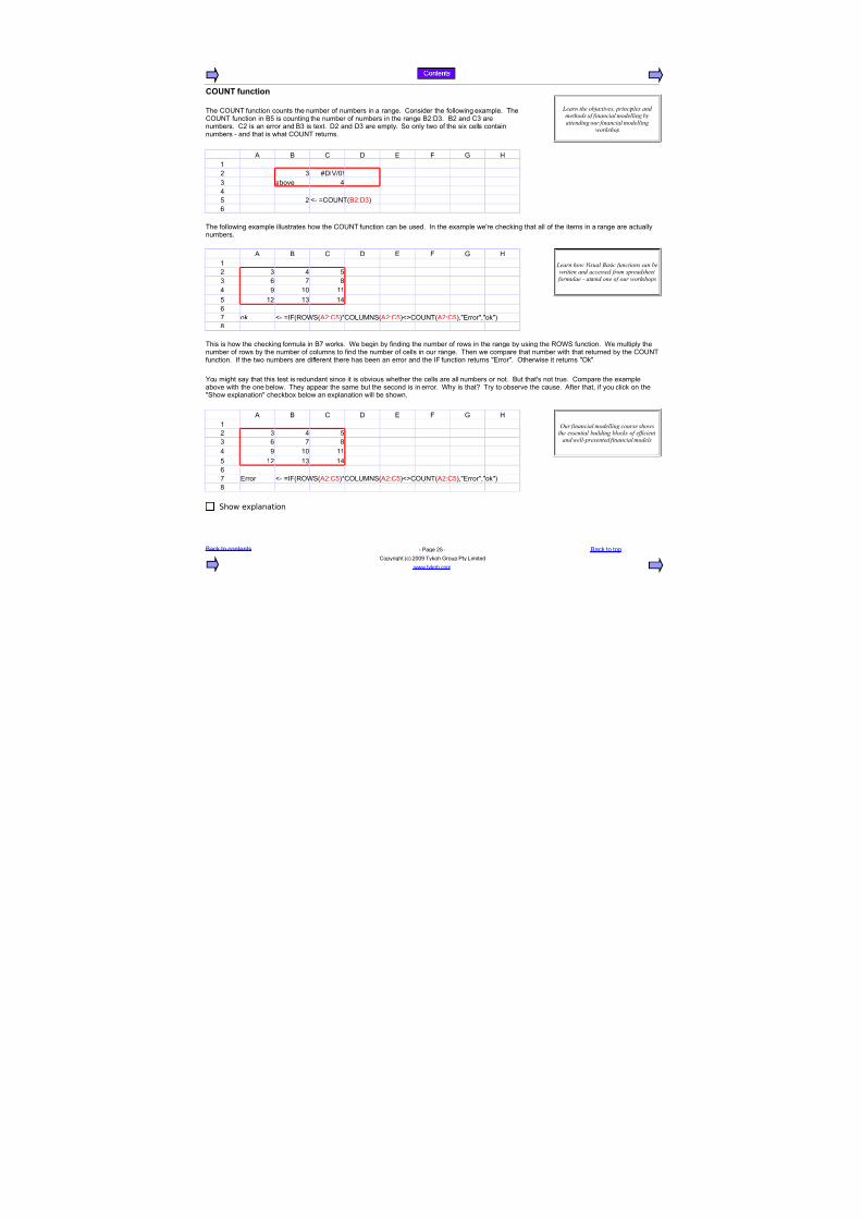
The C2GFT function counts the number of numbers in a range. Consider the following example. TheC2GFT function in &@ is counting the number of numbers in the range &):0!. &) and C! are
numbers. C) is an error and &! is text. 0) and 0! are empty. 4o only two of the six cells containnumbers - and that is what C2GFT returns.
L- OC2GFT&):0!(
The following example illustrates how the C2GFT function can be used. In the example we're checking that all of the items in a range are actuallynumbers.
"earn how Visual Basic functions can bewritten and accessed from spreadsheet
formulae ! attend one of our workshops
L- OI1E2;4 ):C@(/C2,G6F4 ):C@(LMC2GFT ):C@(7rrorok(
This is how the checking formula in &A works. ;e begin by finding the number of rows in the range by using the E2;4 function. ;e multiply thenumber of rows by the number of columns to find the number of cells in our range. Then we compare that number with that returned by the C2GFTfunction. If the two numbers are different there has been an error and the I1 function returns 7rror. 2therwise it returns 2k.
>ou might say that this test is redundant since it is obvious whether the cells are all numbers or not. &ut that's not true. Compare the exampleabove with the one below. They appear the same but the second is in error. ;hy is that< Try to observe the cause. fter that if you click on the4how explanation checkbox below an explanation will be shown.
Our financial modelling course showsthe essential building blocks of efficient
and well!presented financial models
L- OI1E2;4 ):C@(/C2,G6F4 ):C@(LMC2GFT ):C@(7rrorok(
Show explanation
7/18/2019 SpreadsheetGuide_1.02 (1) - copia
http://slidepdf.com/reader/full/spreadsheetguide102-1-copia 50/114
C8?$# function
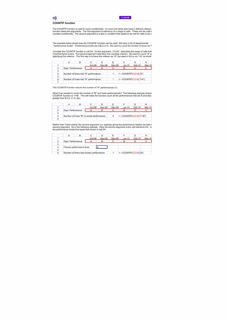
The example below shows how the C2GFTI1 function can be used: ;e have a list of departmental performance levels. $erformance levels are &C or 0. ;e want to count the number of times an
& C 0 7 1 + =
% 2ct-"* Fov-"* 0ec-"* Jan-%" 1eb-%" 6ar-%") 0ept. $erformance: & C & 0 C
!
9 Fumber of times had performance: %
@
Fumber of times had performance: %
A
The C2GFTI1 function returns the number of performances %(.
& C 0 7 1 + =
% 2ct-"* Fov-"* 0ec-"* Jan-%" 1eb-%" 6ar-%"
) 0ept. $erformance: & C & 0 C
!
9 Fumber of times & or worse performance: @
@
& C 0 7 1 + =
% 2ct-"* Fov-"* 0ec-"* Jan-%" 1eb-%" 6ar-%"
) 0ept. $erformance: & C & 0 C
!
9 Choose performance level:
@
Fumber of times had chosen performance: %
The C2GFTI1 function is used to count conditionally - to count only items that meet a defined criterion.function takes two arguments. The first argument is reference to a range of cells. These are the cells t
counted conditionally. The second argument is a test or condition that needs to be met for cells to be c
Consider the C2GFTI1 function in cell 79. Its first argument - C):=) - describes the range of cells thatof performance levels. The second argument describes the counting criterion: ;e want to count pspecifying the criterion. The first way is to have the criterion as as used in 79( or as O as show
L- OC2GFTI1C):=)(
L- OC2GFTI1C):=)O(
;hat if we wanted to count the number of & and lower performances< The following example showsC2GFTI1 function is MO&. This will make the function count all the performances that are & and alsogreater than & i.e. C 0 etc(.
L- OC2GFTI1C):=)MO&(
Eather than hard-coding the second argument i.e. explicitly giving the performance levels( we wish tsecond argument. s in the following example. =ere the second argument is the cell reference 09. Inthe performance levels that e5ual that shown in cell 09.
L- OC2GFTI1C):=)09(

7/18/2019 SpreadsheetGuide_1.02 (1) - copia
http://slidepdf.com/reader/full/spreadsheetguide102-1-copia 51/114
A
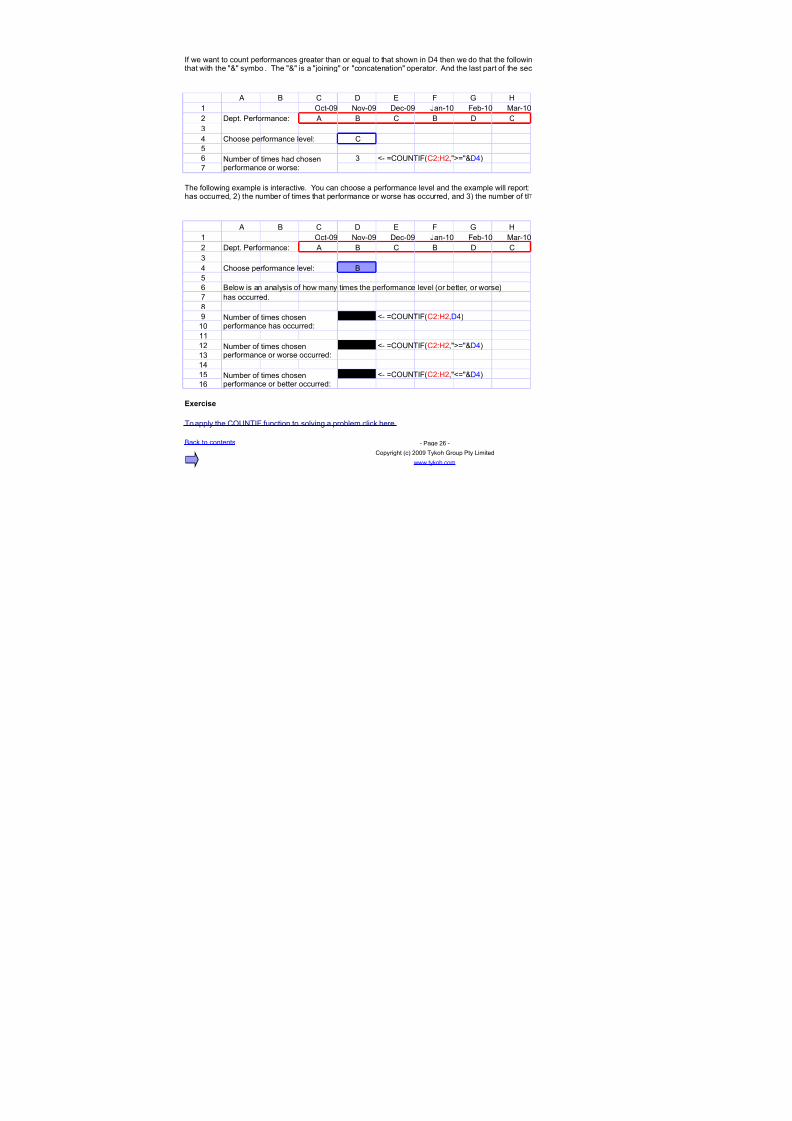
7/18/2019 SpreadsheetGuide_1.02 (1) - copia
http://slidepdf.com/reader/full/spreadsheetguide102-1-copia 52/114
& C 0 7 1 + =
% 2ct-"* Fov-"* 0ec-"* Jan-%" 1eb-%" 6ar-%"
) 0ept. $erformance: & C & 0 C!
9 Choose performance level: C
@
!
A
& C 0 7 1 + =
% 2ct-"* Fov-"* 0ec-"* Jan-%" 1eb-%" 6ar-%"
) 0ept. $erformance: & C & 0 C
!
9 Choose performance level: &
@
&elow is an analysis of how many times the performance level or better or worse(
A has occurred.
8
* )
%"
%%
%) @%!
%9
%@ !
%
.xercise
&ack to contents - $age ) -
Copyright c( )""* Tykoh +roup $ty ,imited
www.tykoh.com
If we want to count performances greater than or e5ual to that shown in 09 then we do that the followinthat with the symbol. The is a oining or concatenation operator. nd the last part of the sec
Fumber of times had chosenperformance or worse:
L- OC2GFTI1C):=)MO09(
The following example is interactive. >ou can choose a performance level and the example will report:has occurred )( the number of times that performance or worse has occurred and !( the number of ti
Fumber of times chosenperformance has occurred:
L- OC2GFTI1C):=)09(
Fumber of times chosenperformance or worse occurred: L- OC2GFTI1C):=)MO09(
Fumber of times chosenperformance or better occurred:
L- OC2GFTI1C):=)LO09(
To apply the C2GFTI1 function to solving a problem click here.

7/18/2019 SpreadsheetGuide_1.02 (1) - copia
http://slidepdf.com/reader/full/spreadsheetguide102-1-copia 53/114
performance has occurred.
"earn how to use iteration$ goal!seeking$the solver and optimisation to solve
problems that are too complex to solve ina single step
Theo be
ounted.
will be counted. These cells contain the listrformances. There are two ways ofin 7.
how to do that. The second argument of theall the performances that are alphabetically
Our workshops review the finance principles and assumptions underlyingthe main spreadsheet financial functions
o count( we can have a cell reference as thethis case the C2GFTI1 function will count all

7/18/2019 SpreadsheetGuide_1.02 (1) - copia
http://slidepdf.com/reader/full/spreadsheetguide102-1-copia 54/114

7/18/2019 SpreadsheetGuide_1.02 (1) - copia
http://slidepdf.com/reader/full/spreadsheetguide102-1-copia 55/114
&ack to top
g way. ;e hard-code the MO and followond argument is the cell reference 09.
%( The number of times that performancees that performance or better has occurred.
Our workshops review the finance principles and assumptions underlyingthe main spreadsheet financial functions

7/18/2019 SpreadsheetGuide_1.02 (1) - copia
http://slidepdf.com/reader/full/spreadsheetguide102-1-copia 56/114
$# function
In the example below the I1 statement's first argument is % M C%. % @( is not greater than C% ( and so the test returns 1,47.
& C 0 7 1 + =
% @
)
! less or e5ual
9
The following example is an interactive version of the one above.
& C 0 7 1 + =% A A
)
!
9
@ less or e5ual
ested or compound $# functions
;e'll look at an example in which one of three results 'greater less and e5ual( is to be returned.
;e will compare two values Dalue % and Dalue )( and determine whether Dalue % is greater than e5ual to or less than Dalue ).
& C 0 7 1 + =
%
) Dalue % Dalue ) Test
! A greater
9
@ e5ual
A @ less
In the formula in CA both of the I1 functions tests return 1,47 and so the third argument of the last I1 function is returned.
The example below is an interactive version of the one above.
& C 0 7 1 + = I J H ,
% Dalue % Dalue ) Test
) A greater
!
9@
Dalue % is greater than Dalue )
&ack to contents - $age )A - &ack to top
Copyright c( )""* Tykoh +roup $ty ,imited
www.tykoh.com
We can customise our courses for particular audience
The I1 function takes three arguments. The first describes a test or condition which should returnTEG7 or 1,47(. If the first argument is true the I1 statement returns its second argument and
otherwise it returns the third argument.
R1or more information about logical tests and conditions click here.S
L- OI1 %MC%greaterless or e5ual(
We can tailor courses to specificaudiences ! eg audiences with a
derivatives focus
L- OI1 %MC%greaterless or e5ual(
s we have seen the I1 function returns one of two results either the second or third argument(. ;hat if we want to return one of three results<2ne way of achieving this is to nest I1 functions - i.e. have one inside the other.
,ook at the formula in C! below. The I1 function in that formula makes the test !M&!. ! is A and &! is . 4o the test is TEG7. 4ince the test istrue the second argument of the I1 function greater( is returned.
Our modelling and spreadsheet skillscourses cover both core and extended
spreadsheet and finance topicsL- OI1 !M&!greaterI1 !O&!e5ualless((
L- OI1 @M&@greaterI1 @O&@e5ualless((
L- OI1 AM&AgreaterI1 AO&Ae5ualless((
Fow look at the formula in C@ above. This time the I1 function's test isn't satisified since @ isn't greater than &@. 4o the third argument of the I1
function is looked at. The third argument is a whole other I1 function OI1@O&@e5ualless(. This function's test is satisfied @ does e5ual &@(and so it returns its second argument e5ual(.
L- OI1 )M&)greaterI1 )O&)e5ualless((
L- ODalue % is I1 )M&)greater thanI1 )O&)e5ual toless than(( Dalue )
RTo carry out an exercise on compound I1s click here.S

7/18/2019 SpreadsheetGuide_1.02 (1) - copia
http://slidepdf.com/reader/full/spreadsheetguide102-1-copia 57/114
$SA function
In cell &) we do a lookup of the table to find the number of staff in 0epartment . The D,22HG$ function in &) works this way:
R1or more information on the D,22HG$ function click S
& C 0 7 1 + = I J H
% 0ept 4taff 0ept 4taff
) !@" " !@"
! 0 %)"
9 C KF % 1 )""
@ + %)
,ookup failed C doesn't exist =
A
$nteractive example
& C 0 7 1 + = I J H% 0ept 4taff ,ocation
) !@" 4ingapore
! 0 %)" uckland
9 1 )"" 4ydney
@ 0ept: + %) Few >ork
= ,ondon
A
8 4taff: !@"
&ack to contents - $age )8 - &ack to top
Copyright c( )""* Tykoh +roup $ty ,imited
www.tykoh.com
Our modelling and spreadsheet skillscourses can be done in one or two day
modules
The I4F function is often used to detect whether lookups have failed. 1ailed lookups are those in which theitem being looked for isn't found. ;e'll illustrate how I4F works by considering an example in which we perform
a lookup on a table containing departmental information.
The departmental table is defined in cells J):H below. The first column of the table is a list of department codesand the second column gives the number of staff for each department. ;e want to do lookups of that table to findthe number of staff for a given department.
The first argument )( specifies what we're looking for. In this case it's . The second argument specifies where we're looking for . In thiscase it's in the departmental table at J):H. The third argument specifies which column of the table we want to retrieve information from. ;e wantthe staff column. Column numbering starts at the leftmost column of the table being searched and so the staff column is column number ). Thelast argument specifies what to do if the item being looked for isn't in the table. If the fourth parameter is 1,47 thenan error KF( is returned ifthe item isn't found. If the fourth parameter is TEG7 or is absent then the nearest item will be found.
here
,ookupstatus
L- OD,22HG$ )J):H)1,47( L- OI4F&)(
L- OD,22HG$ 9J):H)1,47( L- OI4F&9(
L- OI1I4F&9(,ookup failed 9 doesn't exist&9(
The lookup in &) succeeds and returns the number of staff for 0epartment . Fow consider the lookup in cell &9. That lookup fails because C - thedepartment code being looked for - isn't in the department table.
,et's look now at how I4F can detect the status of our lookups. I4F takes a single argument. I4F returns TEG7 if its argument is KF. I4Freturns 1,47 if its argument isn't KF.
The I4F function in +) detects the status of the D,22HG$ in &). That lookup succeeds the value it generates isn't KF and so I4F returns1,47. The I4F function in +9 detects the status of the D,22HG$ in &9. That lookup fails and generates the result KF. In this case I4Freturns TEG7.
n example of how the I4F function can be used is shown in cell above: I1 and I4F are used together to inform the user if the lookup fails.Fote that the error message we generate is much more user friendly and informative than is KF.
Our financial modelling course showsthe essential building blocks of efficient
and well!presented financial modelsThe example below is interactive. >ou can select a department. 0epending on whether or not the selecteddepartment is found and appropriate result is returned.
L- OI1I4FD,22HG$&@+):I)1,47((no match D,22HG$&@+):I)1,47((
D,22HG$ is an expensive function in terms of the load it imposes on computers so it's best to minimise its use. The example above usesD,22HG$ twice in the formula in &8. If many such calculations are to be done its probably better to split the formula into two seperate cells and touse D,22HG$ only once.

7/18/2019 SpreadsheetGuide_1.02 (1) - copia
http://slidepdf.com/reader/full/spreadsheetguide102-1-copia 58/114
(A/B. function
& C 0 7 1 + =
%
) %A ! )A
! -!9 %* 9
9
@ )A
A %A
& C 0 7 1 + = I J H
% Fth largest to show: ) %A ! )A
) -!9 %* 9
!
9
@
A The )nd largest is %*
8
Sorting
& C 0 7 1 + =
% Gnsorted Eank 4orted
) )! % *)
! %A ) A8 L- O,E+7PP):PPA&!(
9 A8 ! % L- O,E+7PP):PPA&9(
@ %) 9 )! L- O,E+7PP):PPA&@(
*) @ %A L- O,E+7PP):PPA&(
A % %) L- O,E+7PP):PPA&A(
+aired sorting
n additional complication is that numbers in the unsorted column can be duplicated. The duplicates may have different pairs.
& C 0 7 1 + =
% Gnsorted $aired 4orted $aired
) %! %) A @
! )@ %A 9@ %*
9 ! !) ! !)
@ 9@ %* )@ %A
% %" )) %A A @ %! %)
8 %! @ %! @
* )) % % %"
&ack to contents - $age )* - &ack to top
Copyright c( )""* Tykoh +roup $ty ,imited
www.tykoh.com
Outsourcing of training functions ! one
of the services we offer
The ,E+7 function returns the largest number from a group. 6ore generally the function returns the Fthlargest number. The function takes two parameters. The first parameter is a reference to a cell or group of cells.
The second parameter is a number that indicates how large. If the second parameter is % then the largestnumber in the range is returned if ) then the second largest is returned and so on.
L- O,E+7 ):C!%(
L- O,E+7 ):C!!(
The following shows interactively how ,E+7 works. In cell C% you choose how large e.g. % O largest ) O second largest etc(. The answer isshown in cell A. In A note how the I1 and C=2247 functions are used to add the st in %st the nd in )nd the rd in !rd and the th
thereafter.
L- OThe C%I1C%M!thC=2247C%stndrd(( largest is ,E+77%:+)C%(
'eedback from our Visual Basic course)%4ood use of examples to solidify
knowledge%
The ,E+7 function can be used to dynamically sort data. The example below gives a simple illustration.
Column contains unsorted data. Column & contains the integers starting at % and increasing by % on eachsuccessive row.
L- O,E+7PP):PPA&)(
Column C contains sorted data and each cell's value is set by a ,E+7 function. The ,E+7 function on the top row has a second argument of %.4o C% is the largest of the numbers in the column. The ,E+7 function on the second row has a second argument of ). 4o C) is the second
largest of the numbers. nd so on. ;e can see that the ,E+7 functions generate a sorted set of data in column C.
1ollowing is a more complex sorting example. Column is unsorted. Column & is 'paired' with column . 4o the %) in cell &) is paired with the %!in cell ). In the sorted columns 0 7 the %) should still be paired with the %!.
Our courses are presentedinternationally

7/18/2019 SpreadsheetGuide_1.02 (1) - copia
http://slidepdf.com/reader/full/spreadsheetguide102-1-copia 59/114
(.#?= M$-= /$B"? and (. functions
?he (.#? function
In the formula in cell &! the ,71T function is provided with a second argument - ). 4o the left ) characters of 1+=)!9 are returned.
& C 0 7 1 +
% 1+=)!9 1
)
! 1+
9
@ 1+=)!9
A
&elow is a simpled example showing the left function being used to abbreviate the names of the months to a standard three character length.
& C 0 7
% January Jan
) 1ebruary 1eb L- O,71T)!(! 6arch 6ar L- O,71T!!(
9 pril pr L- O,71T9!(
@ 6ay 6ay L- O,71T@!(
June Jun L- O,71T!(
A July Jul L- O,71TA!(
8 ugust ug L- O,71T8!(
* 4eptember 4ep L- O,71T*!(
%" 2ctober 2ct L- O,71T%"!(%% Fovember Fov L- O,71T%%!(
%) 0ecember 0ec L- O,71T%)!(
?he /$B"? function
& C 0 7 1
% Fumber characters returned from the string: %
)
! Text: This is a long piece of text
9
@ Eesult: t
?he M$- function
& C 0 7 1 + =
% 4tart position: )
)
! Fumber characters: 9
9
@
4tring: &C071
A
8 Eesult: &C07
'eedback from our 'inancial (odellingcourse) %*nderstanding the complex
Excel tips was very beneficial% The ,71T function works with strings - text in other words. The ,71T function can takeone or two arguments. The first argument is a string. If there isn't a second argument thenthe ,71T function returns the leftmost character in its first argument. This is illustrated inthe example below.
,ook at the formula in cell &%. The ,71T function's single argument is % % contains1+=)!9. &ecause the ,71T function isn't provided with a second argument it returns theleftmost character of 1+=)!9 i.e. 1.
If the second argument is larger than the number of characters in the first argument then the ,71T function returns all of the first argument - asshown by the formula in cell &@.
L- O,71T %(
L- O,71T %)(
L- O,71T %)"(
'eedback from our 'inancial (odelling
course) %-he V will be very helpful5%
L- O,71T %!(
R1or a more complex example using the ,71T function click here.S
The EI+=T function works much the same as the ,71T function except that it takes the rightmost characters of a string. The following interactiveexample lets you choose the number of characters returned by the EI+=T function.
L- OEI+=T&!7%(
The 6I0 function returns the middle characters in a string. The function takes three arguments. The first argument is the string whose middle isbeing found. The second argument specifies the position of the first character that will be returned character numbering starts at %(. The thirdparameter is the length of the returned string.
L- O6I0& C% C!(

7/18/2019 SpreadsheetGuide_1.02 (1) - copia
http://slidepdf.com/reader/full/spreadsheetguide102-1-copia 60/114
(8+ function
There are two forms of the ,22HG$ function - a Dector form - and an array form. In this section we'll look only at the Dector form.
&elow is an example showing the vector form of the ,22HG$ function. This form takes three arguments.
- The first argument specifies what is being looked for. In this case we're looking for a tax code of & specified in cell !(.
- The second argument specifies which column or row( is being searched. In this case we're searching column 1.
- The third argument is the result column or row( and contains the values the lookup will return.
If the lookup finds what it's looking for in the second position in the search column then it will return the second entry from the result column.
& C 0 7 1 + =%
) Tax code Eate Code Eate
! & %@# @#
9 & %@#
@ C !@#
0 9)#
A 7 9A#
8
& C 0 7 1 + =
% Eate
) Tax code Eate @#
! & %@# %@# Code
9 !@#
@ 9)# &
9A# C
A 0
8 7
nd in the following example the search and result both have a horiNontal orientation.
& C 0 7 1 + =
% Eate @# %@# !@# 9)# 9A#
)
! Code & C 0 7
9
@ Tax code Eate
& %@#
A
8
nd in this example the search is horiNontal and the result is vertical.
& C 0 7 1 + =
% Code & C 0 7 Eate
) @#
! %@#
9 !@#
@ Tax code Eate 9)# & %@# 9A#
A
8
Our modelling and spreadsheet skillscourses can be done in one or two day
modules
vervie!The ,22HG$ function performs a lookup on a table that has either a vertical organisation i.e. in
columns( or a horiNontal organisation i.e. in rows(. nother function in the looking-up family -D,22HG$ - works only with tables in a vertical organisation. nd =,22HG$ works only with tablesthat have a horiNontal organisation.
L- O,22HG$ !1!:1A=!:=A(
&oth the search column and the result column should be only one column wide. There is no re5uirement - unlike with D,22HG$ - to have the resultcolumn in any particular position relative to the search column. Consider the following example where they're back to front and offset.
L- O,22HG$ !=9:=81):1(
"earn how to choose the best function to solve a problem when several functions
are available by attending one of ourworkshops
L- O,22HG$ &!:1!&%:1%(
L- O,22HG$ &%:1%=):=(

7/18/2019 SpreadsheetGuide_1.02 (1) - copia
http://slidepdf.com/reader/full/spreadsheetguide102-1-copia 61/114
& C 0 7 1 + =
%
) Tax code Eate Code Eate! & @# @#
9 C %@#
@ 0 !@#
7 9)#
A 1 9A#
8
Fote that ,22HG$ will return an error if the first entry in the search column is larger than the item being looked up. s in the following example.
& C 0 7 1 + =
%
) Tax code Eate Code Eate
! KF & @#
9 C %@#
@ 0 !@#
7 9)#
A 1 9A#
8
The item being looked for is . The first item in search column 1 is &. nd the ,22HG$ fails.
& C 0 7 1 + =
%
) Tax code Eate Code Eate
! C %@# & @#
9 C %@#
@ 7 !@#
1 9)#
A + 9A#
8
&ack to contents - $age !% - &ack to top
Copyright c( )""* Tykoh +roup $ty ,imited
www.tykoh.com
The ,22HG$ function isn't as flexible as the D,22HG$ function in terms of allowing you to specify whether or not you want an exact match.,22HG$ always returns a nearest match. s in the following example.
'eedback from our ,preadsheet skills
course) %Excellent knowledge and clearcommunication from the presenter% L- O,22HG$ !1!:1A=!:=A(
& - the item being searched for - isn't in the search column. 4o the nearest result the one for ( is returned.
1or this to work reliably the search column must be in sorted ascending order.
4ee the description of the D,22HG$ function for an outline of how ,22HG$ D,22HG$ and =,22HG$ searching works to find the nearestresult.
L- O,22HG$ !1!:1A=!:=A(
The following example lets you experiment with the ,22HG$ function. The cell with a blue background can be changed. The output is the cellwith the black background.
Our courses are presentedinternationally
L- O,22HG$ !1!:1A=!:=A(

7/18/2019 SpreadsheetGuide_1.02 (1) - copia
http://slidepdf.com/reader/full/spreadsheetguide102-1-copia 62/114
MA?C" function
?hird argument of * % exact match re0uired
In the example below is found in the first position of the search list so the 6TC= function returns %The 6TC= function in cell @ searchs for &. & is fifth in the search list and so the function returns
& C 0 7 1 + =
%
) C 1 + &
!
9 %
@ @
KF
A
?hird argument of 1 % nearest match in ascending list
& C 0 7 1 + =
%
) & C 7 + I
!
The 6TC= function searches for a specified item in a list and returns the position of the item. 1orexample if the item is found in the first position of the list the 6TC= function will return %.
The 6TC= function takes three arguments. The first argument specifies what is being searched forthe second item specifies the row or column that is searched and the last argument determines thekind of search done.
Consider the example shown below. ,ook at the 6TC= function in cell 9. The first argument is .The second argument is PCP):P+P). This specifies the cells the 6TC= function will search. 4o the fPCP):P+P). The third argument is ". The third argument specifies whether 6TC= returns an error ifit returns the nearest it can find. third argument of " - as in this case - re5uires the function to returnexact match.
In cell the 6TC= function searches for 0. =owever 0 isn't in the search list and because theand one isn't found an error is returned.
L- O6TC=PCP):P+P)"(
L- O6TC=&PCP):P+P)"(
L- O6TC=0PCP):P+P)"(
If the third argument of the 6TC= is a % then the function will return the nearest match it can find. 1osearch list must be sorted in ascending order. The example below shows how the 6TC= function w
If there is an exact match the function will return the position of the 6TC=. This case is shown in celland finds it in the second position.
The formula in cell @ shows what happens if the item being searched for isn't found. 1 is being searreturns ! which is the position of 7 in the list. 4o the 6TC= function when the third argument is %(less than or e5ual to what is being searched for.
The formula in cell shows what happens when the item being searched for is less than - i.e. before -returned.

7/18/2019 SpreadsheetGuide_1.02 (1) - copia
http://slidepdf.com/reader/full/spreadsheetguide102-1-copia 63/114
9 )
@ !
KF
A
L- O6TC=CPCP):P+P)%(
L- O6TC=1PCP):P+P)%(
L- O6TC=PCP):P+P)%(
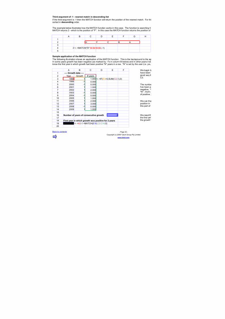
7/18/2019 SpreadsheetGuide_1.02 (1) - copia
http://slidepdf.com/reader/full/spreadsheetguide102-1-copia 64/114
?hird argument of %1 % nearest match in descending list
& C 0 7 1 + =
%
) = 1 C &
!
9 )
@
Sample application of the MA?C" function
& C 0 7 1
% %%%% Bro!th data %%%%
) >ear +rowth K years
! %**8 % %."""
9 %*** -% "."""@ )""" -% ".""" )""% % %."""A )"") % )."""8 )""! -% "."""* )""9 -% "."""
%" )""@ % %."""%% )"" % )."""%) )""A % !."""%! )""8 -% "."""
%9 )""* % %."""
%@
% umber of 'ears of consecutive gro!th )
%A
%8 #irst 'ear in !hich gro!th !as positive for 2 'ears
%* )"")
)"
&ack to contents - $age !) -Copyright c( )""* Tykoh +roup $ty ,imited
www.tykoh.com
If the third argument is -% then the 6TC= function will return the position of the nearest match. 1or thisorted in descending order.
The example below illustrates how the 6TC= function works in this case. The function is searching f6TC= returns ) - which is the position of 1. In this case the 6TC= function returns the position of
L- O6TC=0PCP):P+P)-%(
The following illustration shows an application of the 6TC= function. This is the background to the apIn some years growth has been negative as marked by -%'s in column & below( and in other years it wknow the first year in which growth had been positive F years in a row. F is set by the user i.e. you
;e begin bhave beengood way tC!.
L- OI1&!M"4G6C)%("(
The numbehas been pnegative.F - that'sof positive
;e can theposition inthis part of
;e need tthe f irst yethe growth
L- O !-% Q6TC=7%C!:C%9"(

7/18/2019 SpreadsheetGuide_1.02 (1) - copia
http://slidepdf.com/reader/full/spreadsheetguide102-1-copia 65/114
- the position of the in the list.@.
Exercises in our spreadsheet skills andmodelling courses give you instant
feedback of your progress
4o the 6TC= function will search for .unction will search for in the cellsit doesn't find what it's looking for or whethern exact match or an error if it cannot find an
TC= is re5uired to find an exact match
.onsulting on spreadsheet$ modellingand &uantitative issues ! a service we
offer
the function to work reliably in this case therks in this case.
9 below. The 6TC= is searching for C
hed for but isn't in the list. The 6TC=eturns the position of the largest item that is
the first item in the search list: n error is
'eedback from our 'inancial (odellingcourse) %*nderstanding the complex
Excel tips was very beneficial%

7/18/2019 SpreadsheetGuide_1.02 (1) - copia
http://slidepdf.com/reader/full/spreadsheetguide102-1-copia 66/114

7/18/2019 SpreadsheetGuide_1.02 (1) - copia
http://slidepdf.com/reader/full/spreadsheetguide102-1-copia 67/114
&ack to top
s to work reliably the search list must be
r 0 but 0 isn't in the search list. Thethe smallest item that is greater than or e5ual
'eedback from our ,preadsheet skillscourse) %-he facilitator is an excellentresource -hanks for the opportunity to
complete this%
plication. ;e have a set of growth figures.s positive as marked by %'s(. ;e want toin cell 7%.
y working out a way to determine when thereF consecutive years of positive growth.
do that is as shown by the formula in cell
r in column C increases by % when growthositive and resets to Nero when growth is
hen the number in the C column reacheswhen there have been F consecutive yearsrowth.
n use the 6TC= function to find the firstolumn C of F. That is done in cell %* in
the formula: MA?C"9.1=C3:C14=*;
add the position returned by the 6TC= tor less %( to obtain the actual year in whichwas positive F times.
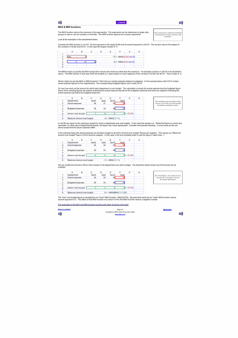
7/18/2019 SpreadsheetGuide_1.02 (1) - copia
http://slidepdf.com/reader/full/spreadsheetguide102-1-copia 68/114
MAD E M$ functions
,ook at the examples in the spreadsheet below.
& C 0 7 1 + =
%
) limit -) %A
!
9 @ %A %) -)
@
& C 0 7 1 + =
% 0eptartment Forth 7ast 4outh ;est
) ctual expenses ! !A 9! %8
!
9 &udgeted expenses !@ !! 9 %*
@
mount over budget % 9 -! -%
A
8 6aximum amount over budget 9
& C 0 7 1 + =% 0eptartment Forth 7ast 4outh ;est
) ctual expenses !9 !) 9! %8
!
9 &udgeted expenses !@ !! 9 %*
@
mount over budget -% -% -! -%
A
8 6aximum amount over budget -%
& C 0 7 1 + =
% 0eptartment Forth 7ast 4outh ;est) ctual expenses !9 !) 9! %8
!
9 &udgeted expenses !@ !! 9 %*
@
mount over budget -% -% -! -%
A
8 6aximum amount over budget "
Our presenter has conducted workshops
internationally in many countries andcontinents
The 63 function returns the maximum of its arguments(. The arguments can be references to single cells
groups of cells or can be numbers or formulae. The 63 function ignores non-numeric arguments.
Consider the 63 function in cell 7). Its first argument is the range ):&) and its second argument is 9:C9. The function returns the largest ofthe numbers in ):&) and 9:C9. In this case the largest number is %A.
L- O63 ):&) 9:C9(
L- O6IF ):&) 9:C9(
The 6IF function is ust like the 63 except that it returns the minimum rather than the maximum. n example is shown in cell 79 in the illustrationabove. The 6IF function in that case finds the smallest i.e. least positive or most negative( of the numbers in ):&) and 9:C9. That number is -).
;here might we use the 63 or 6IF functions< ;e'll look at a simple example relating to budgeting. In the example below cells C):1) containactual expense figures for four departments. The corresponding budgeted figures are in cells C9:19.
2n row we work out the amount by which each department is over budget. The calculation is simply the actual expense less the budgeted figure.4ome of the resulting figures are positive indicating the actual expense was above the budgeted expense( and some are negative indicating theactual expense was below the budgeted expense(.
Our modelling and spreadsheet skillscourses cover both core and extended
spreadsheet and finance topics
L- O1)-19
L- O63C:1(
In cell 08 we report on the maximum amount by which a department was over budget. In this case the answer is 9. ;hilst that figure is correct andresonable for other sets of departmental figures the figure may not be appropriate. Consider the example following. It is the same as the oneabove except that the actual expenses differ.
In the example below the actual expenses are all below budget so all of the amount over budget figures are negative. This causes our 6aximumamount over budget figure in 08 to become negative. In this case in 08 we'd probably prefer to see the figure " rather than -%.
L- O1)-19
L- O63C:1(
;e can modify the formula in 08 so that it shows " if all departments are within budget. The illustration below shows how the formula can bemodified.
Our Visual Basic course shows how toincrease the %wow!factor% of your
developed applications
L- O1)-19
L- O6363C:1("(
The raw over-budget figure is calculated by an inner 63 function - 63C:1(. ;e pass that result into an outer 63 function whosesecond argument is ". The effect of that 63 function is to return " if the first 63 function returns a negative number.
R1or examples of the 63 and 6IF functions working with other functions click hereS

7/18/2019 SpreadsheetGuide_1.02 (1) - copia
http://slidepdf.com/reader/full/spreadsheetguide102-1-copia 69/114
##S.? function
4eries to chart
4eries nam 0ata
! 9 9 9A& %@ 8) %! )@
C )) 99 %! *! 4eries &
0 % @ A 88
7 A) * %A )A %@ 8)1 !% )8 9A )!
##S.? fundamentals % ##S.? !ith three arguments
& C 0 7 1 + =
% 6cenario 1 2 < >
) +rowth %)# %9# %"# %%#
!
9 Chosen scenario
@ 4cenario number: !
vervie!
Gsually when you write a formula you hard-code which cells the formula will reference. formula migO4G6P+@:=A(. The P+@:=A is a hard-coded cell reference. &y hard-coded we mean that the cellis set explicitly at the time the formula is written.
&ut sometimes you can't hard-code which cells to reference. Consider the chart shown below for exam through 1(. ;hich of the six series is charted is determined by the user i.e. you( making a selection
In the chart we obviously can't hard-code a reference to a particular data series. That is because the ldepending on the user's selection. 4ituations like this are where the 21147T function is useful: Thedynamic cell references based on changing criteria.
In its simplest version the 21147T function takes three arguments. ;e'll illustrate by using the followito select one of four scenarios. The scenarios are defined in the cells shown with a light yellow backgroC below.
The 21147T function's first argument is a base or starting position - ) in this case.
The second argument specifies a row offset - it defines how many rows down to move from the base pwe don't move any rows away from the base i.e. we stay on row )(.
The third argument specifies a column offset - it defines how many columns to the right we move from toffset is determined by the number in C@. The number in C@ is !. 4o we move three columns to the ri
%
"
)"
9"
"
8"
%""

7/18/2019 SpreadsheetGuide_1.02 (1) - copia
http://slidepdf.com/reader/full/spreadsheetguide102-1-copia 70/114
+rowth: %"#
A
L- O21147T )"C@(
=aving started at ) moved down Nero rows and moved across C@ columns we arrive at cell 0). Therate in 0)( is shown in the chosen scenario growth rate cell C(. If the chosen scenario had been 9 trate shown in C. ;e can see that the 21147T function lets the user select a scenario growth rate by
+ositive and negative offsets
The second and third arguments of the 21147T function can be negative or positive. positive row ofa negative offset is up the page. positive column offset is a movement to the right and a negative off
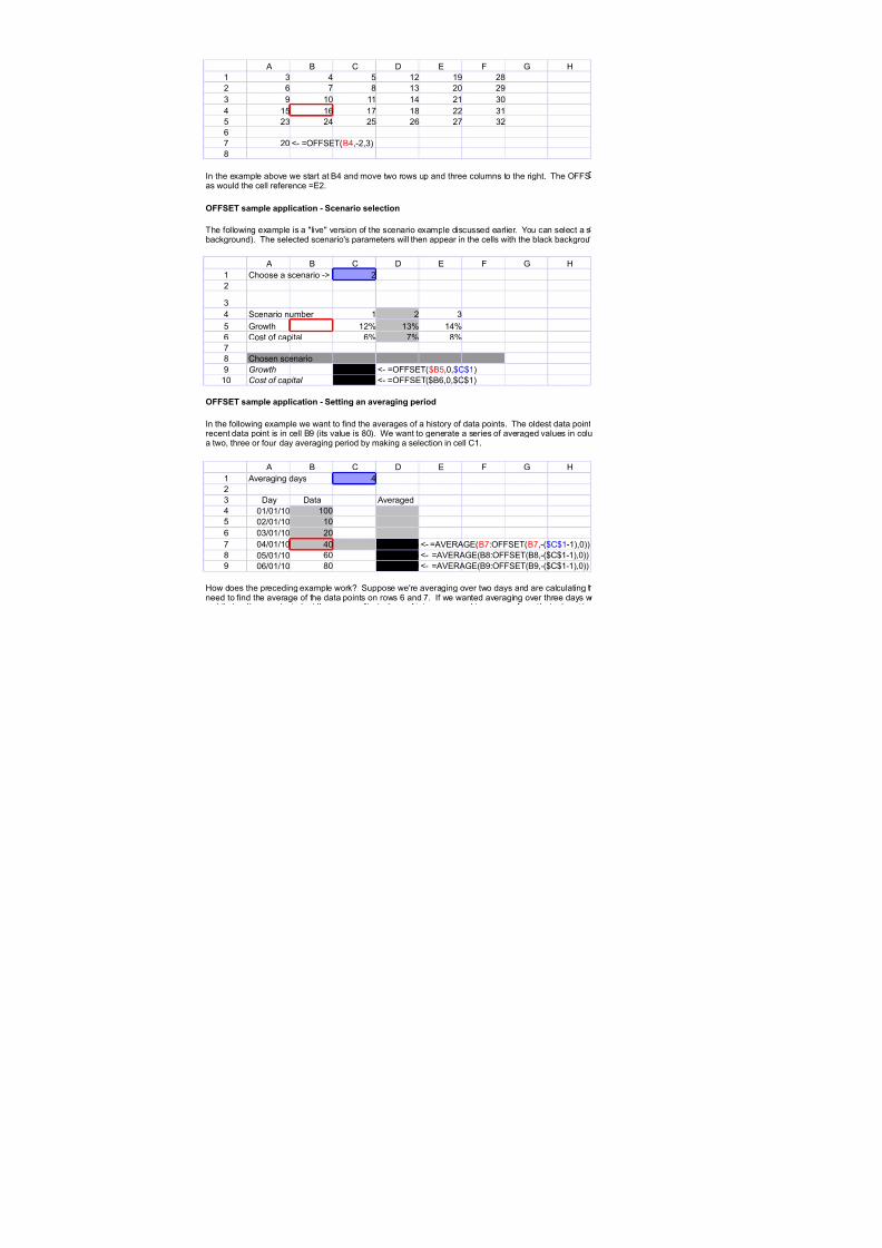
7/18/2019 SpreadsheetGuide_1.02 (1) - copia
http://slidepdf.com/reader/full/spreadsheetguide102-1-copia 71/114
& C 0 7 1 + =
% ! 9 @ %) %* )8
) A 8 %! )" )*
! * %" %% %9 )% !"
9 %@ % %A %8 )) !%
@ )! )9 )@ ) )A !)
A )"
8
##S.? sample application % Scenario selection
& C 0 7 1 + =
% Choose a scenario -M )
)
!
9 4cenario number % ) !
@ +rowth %)# %!# %9#
Cost of capital # A# 8#
A
8 Chosen scenario
* "ro(th %!#
%" Cost of capital A# L- O21147TP&"PCP%(
##S.? sample application % Setting an averaging period
& C 0 7 1 + =
% veraging days 9
)
! 0ay 0ata veraged
9 "%"%%" %""
@ ")"%%" %"
"!"%%" )"
A "9"%%" 9" 9).@
8 "@"%%" " !).@ L- OD7E+7&8:21147T&8-PCP%-%("((
* ""%%" 8" @"." L- OD7E+7&*:21147T&*-PCP%-%("((
L- O21147T&9-)!(
In the example above we start at &9 and move two rows up and three columns to the right. The 2114as would the cell reference O7).
The following example is a live version of the scenario example discussed earlier. >ou can select a sbackground(. The selected scenario's parameters will then appear in the cells with the black backgrou
L- O21147TP&@"PCP%(
In the following example we want to find the averages of a history of data points. The oldest data pointrecent data point is in cell &* its value is 8"(. ;e want to generate a series of averaged values in colua two three or four day averaging period by making a selection in cell C%.
L- OD7E+7&A:21147T&A-PCP%-%("((
=ow does the preceding example work< 4uppose we're averaging over two days and are calculating tneed to find the average of the data points on rows and A. If we wanted averaging over three days w
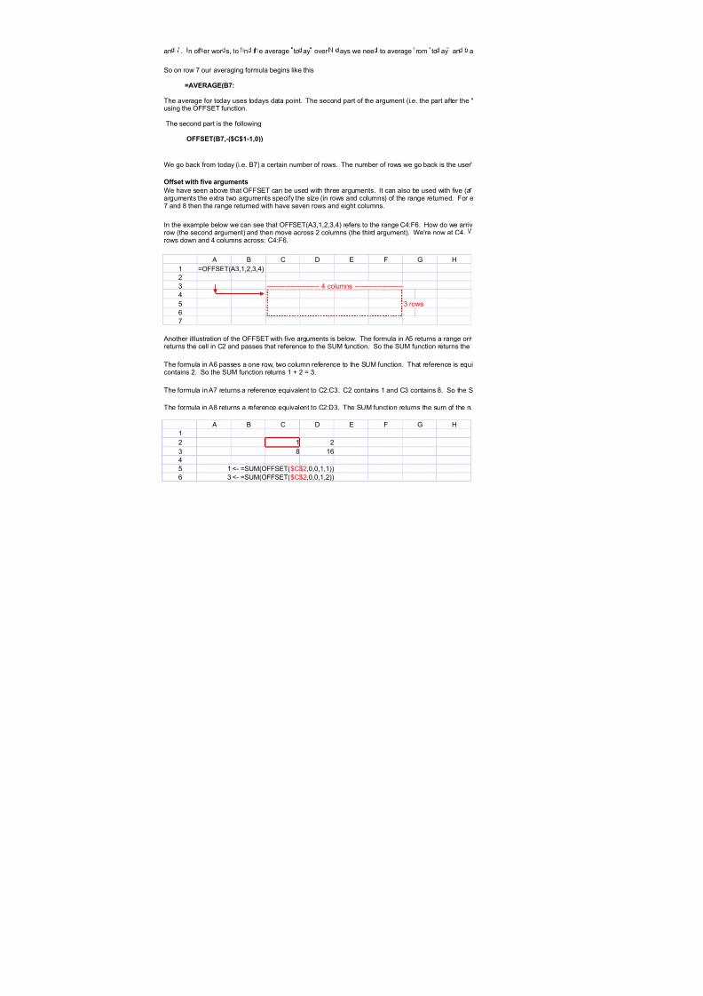
7/18/2019 SpreadsheetGuide_1.02 (1) - copia
http://slidepdf.com/reader/full/spreadsheetguide102-1-copia 72/114
;e go back from today i.e. &A( a certain number of rows. The number of rows we go back is the user'
ffset !ith five arguments
& C 0 7 1 + =
% O21147T!%)!9(
)
! ------------------------ 9 columns ----------------------
9
@ ! rows
A
The formula in A returns a reference e5uivalent to C):C!. C) contains % and C! contains 8. 4o the 4
The formula in 8 returns a reference e5uivalent to C):0!. The 4G6 function returns the sum of the n
& C 0 7 1 + =
%
) % )
! 8 %
9
@ %
!
an . n ot er wor s to n t e average to ay over ays we nee to average rom to ay an a
4o on row A our averaging formula begins like this
6A./AB.9,:
The average for today uses todays data point. The second part of the argument i.e. the part after the using the 21147T function.
The second part is the following
##S.?9,=%9FCF1%1=*;;
;e have seen above that 21147T can be used with three arguments. It can also be used with five aarguments the extra two arguments specify the siNe in rows and columns( of the range returned. 1or e
A and 8 then the range returned with have seven rows and eight columns.
In the example below we can see that 21147T!%)!9( refers to the range C9:1. =ow do we arrivrow the second argument( and then move across ) columns the third argument(. ;e're now at C9.rows down and 9 columns across: C9:1.
nother illlustration of the 21147T with five arguments is below. The formula in @ returns a range onreturns the cell in C) and passes that reference to the 4G6 function. 4o the 4G6 function returns the
The formula in passes a one row two column reference to the 4G6 function. That reference is e5uicontains ). 4o the 4G6 function returns % Q ) O !.
L- O4G621147TPCP)""%%((
L- O4G621147TPCP)""%)((

7/18/2019 SpreadsheetGuide_1.02 (1) - copia
http://slidepdf.com/reader/full/spreadsheetguide102-1-copia 73/114
A *
8 )A
*
& C 0 7 1 + =
% veraging days !
)
! 0ay 0ata veraged
9 "%"%%" %""
@ ")"%%" %"
"!"%%" )"
A "9"%%" 9" 9"."
8 "@"%%" " "." L- OD7E+721147T&8""-PCP%-%(%((
* ""%%" 8" 8"." L- OD7E+721147T&*""-PCP%-%(%((
&ack to contents - $age !9 -
Copyright c( )""* Tykoh +roup $ty ,imited
www.tykoh.com
L- O4G621147TPCP)"")%((
L- O4G621147TPCP)""))((
The example below is a practical application of the five-argument version of the 21147T function. It spage - but in a different way.
;e want to find the average of F numbers. >ou can set F to be ) ! or 9. Fow look at the formula isee that the fourth argument of the 21147T function is linked to cell C% - the user's choice of F. 4o tpasses a different siNed column of cells to the D7E+7 depending on the user's choice.
L- OD7E+721147T&A""-PCP%-%(%((

7/18/2019 SpreadsheetGuide_1.02 (1) - copia
http://slidepdf.com/reader/full/spreadsheetguide102-1-copia 74/114
)
%! )@
Our modelling and spreadsheet skills
courses can be done in one or two daymodules ht beeference
le. The chart shows one of six data seriesin the blue area below.
ocation of the relevant series will change1147T function allows us to construct
g example in which a user needs to be ableund. Fow look at the 21147T formula in cell
sition. In this case the row offset is Nero so
he base position. In this case the columnht from the base position.
We can tailor courses to specificaudiences ! eg audiences with a
derivatives focus
) ! 9
4eries &

7/18/2019 SpreadsheetGuide_1.02 (1) - copia
http://slidepdf.com/reader/full/spreadsheetguide102-1-copia 75/114
esult of all this is that scenario !'s growthen it would have been scenario 9's growthtyping the scenario's number into C@.
set defines a movement down the page andet is a movement to the left.

7/18/2019 SpreadsheetGuide_1.02 (1) - copia
http://slidepdf.com/reader/full/spreadsheetguide102-1-copia 76/114
I
Our modelling and spreadsheet skillscourses cover both core and extended
spreadsheet and finance topics
T function in this case generates the same
enario number in the cell with the blued.
2articipants on our courses have theopportunity to do on!line pre and post!
course self!evaluations
is in cell &9 its value is %""(. The mostmn 0. ;e want the user to be able to select
e average value for row A. To do that we'd need to average the data on rows @

7/18/2019 SpreadsheetGuide_1.02 (1) - copia
http://slidepdf.com/reader/full/spreadsheetguide102-1-copia 77/114
s selection in PCP% less %.
G6 function returns *.
mbers in C):0!.
:( needs to be dynamically calculated by
d four( arguments. In the case of fivexample if the fourth and fifth arguments are
e at C9:1< ;e start at ! and go down %e then return a range starting at C9 that is !
Our Visual Basic course shows how toextend or change (icrosoft Office
products6 functionality
row by one columns starting at C). 4o italue of C) %(.
valent to C):0). C) contains % and 0)

7/18/2019 SpreadsheetGuide_1.02 (1) - copia
http://slidepdf.com/reader/full/spreadsheetguide102-1-copia 78/114
I
&ack to top
lves a problem discussed earlier on this
n 0A below. ;e canhe 21147T function

7/18/2019 SpreadsheetGuide_1.02 (1) - copia
http://slidepdf.com/reader/full/spreadsheetguide102-1-copia 79/114
S8M function
& C 0 7 1 +
%
) Fum % @
!
9 Fum ) !
@
4um %)
A
In the example below the 4G6 function adds the numbers in two blocks of cells &):0) and &9:C9( together with the number in the single cell &(.
& C 0 7 1 +
%
) +roup % % ) 9
!
9 +roup ) 8 %
@
Fum ! !)
A
8 4um !
-ifferences bet!een S8M and explicit addition
& C 0 7 1 + =
%
) Dalue Dalue
! % % % KD,G7?
9 ) ! ) KD,G7?
@ 9 A 9
& C 0 7 1 + =
%
) Fum % @ L- @
!
9 Fum ) !
@
4G6: !
A
8 7xplicit addition: 8
The reason explicit addition returns the 8 in C8 is that explicit addition promotes text to numbers if the text is interpretable as being a number.
&ack to contents - $age !@ - &ack to top
Copyright c( )""* Tykoh +roup $ty ,imited
Our Visual Basic course shows how to
extend or change (icrosoft Office products6 functionality
The 4G6 function takes up to thirty arguments. 7ach argument describes a number cell or block of
cells to add up. In the following example the 4G6 function adds the numbers in two cells &) and &9and the number 9(.
L- O4G6&)&9 9(
Our Visual Basic course shows how toautomate routine work and save the timeand trouble of doing the same thing over
and over
L- O4G6&):0)&9:C9&(
4G6 interprets cells that contain text as being Nero. 4o for example 4G6 column title( would be . n example of this behaviour is shownbelow.
In column & we are accumulating a running total. In cell &! we add the current value in cell !( to the previous running total in the row above.;hen we do this in the f irst row we pick up the column title rather than a real running total. =owever since 4G6 interprets text as being Nero thisworks as it should.
Fote that an alternative method of accumulating the running total by explicit addition - as shown in column 1( generates errors when text is addedto numbers.
Our Visual Basic course shows how tointegrate workflows across (icrosoft
Office applications
Eunningtotal
Eunningtotal
L- O4G6 !&)( L- O7!Q1)
nother difference between 4G6 and explicit addition is shown below. &oth the 4G6 formula in C( and the explicit addition formula in C8( areadding cells &) and &9. &ut the two answers are different: 4G6 returns ! and explicit addition returns 8. The reason is that 4G6 interprets cell &)as Nero.
The reason it does that is that &) actually contains text rather than a number: leading apostrophe '( marks the cell as text. nd as we have seenearlier 4G6 interprets text as Nero.
Our workshops review the finance principles and assumptions underlying
the main spreadsheet financial functions
L- 4G6&)&9(
L- O&)Q&9
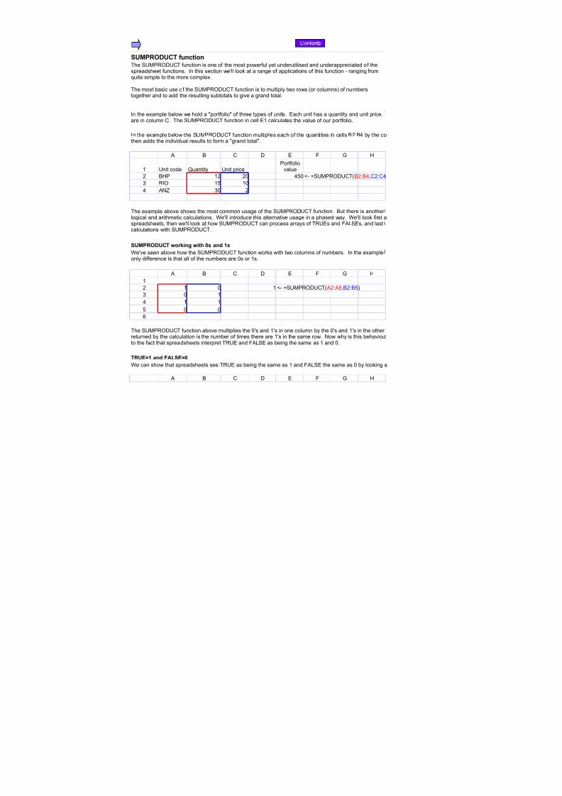
7/18/2019 SpreadsheetGuide_1.02 (1) - copia
http://slidepdf.com/reader/full/spreadsheetguide102-1-copia 80/114
S8M+/-8C? function
& C 0 7 1 + =
% Gnit code Buantity Gnit price
) &=$ %) )" 9@"
! EI2 %@ %"
9 FU !" )
S8M+/-8C? !orking !ith *s and 1s
& C 0 7 1 + =
%
) % " %
! " %
9 % %
@ " "
?/8.61 and #A(S.6*
;e can show that spreadsheets see TEG7 as being the same as % and 1,47 the same as " by looking a
& C 0 7 1 + =
The 4G6$E20GCT function is one of the most powerful yet underutilised and underappreciated of thespreadsheet functions. In this section we'll look at a range of applications of this function - ranging from5uite simple to the more complex.
The most basic use of the 4G6$E20GCT function is to multiply two rows or columns( of numberstogether and to add the resulting subtotals to give a grand total.
In the example below we hold a portfolio of three types of units. 7ach unit has a 5uantity and unit price.are in column C. The 4G6$E20GCT function in cell 7% calculates the value of our portfolio.
In the example below the 4G6$E20GCT function multiplies each of the 5uantities in cells &):&9 by the cothen adds the individual results to form a grand total.
$ortfoliovalue
L- O4G6$E20GCT&):&9C):C9
The example above shows the most common usage of the 4G6$E20GCT function. &ut there is anotherlogical and arithmetic calculations. ;e'll introduce this alternative usage in a phased way. ;e'll look first aspreadsheets then we'll look at how 4G6$E20GCT can process arrays of TEG7s and 1,47s and lastcalculations with 4G6$E20GCT.
;e've seen above how the 4G6$E20GCT function works with two columns of numbers. In the exampleonly difference is that all of the numbers are "s or %s.
L- O4G6$E20GCT ):@&):&@(
The 4G6$E20GCT function above multiplies the "'s and %'s in one column by the "'s and %'s in the otherreturned by the calculation is the number of times there are %'s in the same row. Fow why is this behaviouto the fact that spreadsheets interpret TEG7 and 1,47 as being the same as % and ".

7/18/2019 SpreadsheetGuide_1.02 (1) - copia
http://slidepdf.com/reader/full/spreadsheetguide102-1-copia 81/114
%
) % )
!
9 " %
@
S8M+/-8C? !orking !ith ?/8.s and #A(S.s
L- O )Q%
L- O 9Q%
Cell ) contains the value TEG7. Cell &) contains the formula O)Q%. 4ince cell &) returns ) we can conas being the same as %.
Cell 9 contains the value 1,47. Cell &9 contains the formula O9Q%. 4ince cell &9 returns % we can co1,47 as being gthe same as ".
The example below is very similar to the example shown in the earlier section 4G6$E20GCT working witdifferences:
The first difference is that %s have been replaced by TEG7s and "s by 1,47s. The second difference is4G6$E20GCT arguments has been replaced by a multiplication sign /(.
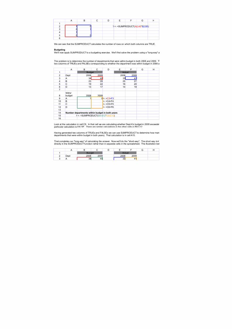
7/18/2019 SpreadsheetGuide_1.02 (1) - copia
http://slidepdf.com/reader/full/spreadsheetguide102-1-copia 82/114
& C 0 7 1 + =
%
) % " %
! " %
9 %
@ " "
;e can see that the 4G6$E20GCT calculates the number of rows on which both columns are TEG7.
,udgeting
;e'll now apply 4G6$E20GCT to a budgeting exercise. ;e'll first solve the problem using a long-way a
& C 0 7 1 + =
% &udget ctual
) 0ept )""8 )""* )""8 )""*
! !9 9" !! 9%
9 & )! )8 )@ )A
@ C %* )) % )"
0 %! %A %9 %*
A
8 )""8 )""*
* % "
%" & L- OC9M19%% C L- OC@M1@
%) 0 L- OCM1
%!
%9 umber departments !ithin budget in both 'ears
%@ %
%
& C 0 7 1 + =
% &udget ctual
) 0ept )""8 )""* )""8 )""*
! !9 9" !! 9%
L- O4G6$E20GCT ):@/&):&@(
The problem is to determine the number of departments that were within budget in both )""8 and )""*. Ttwo columns of TEG7s and 1,47s corresponding to whether the department was within budget in )""8 a
;ithinbudget
L- OC!M1!
L- O4G6$E20GCT&*:&%)/C*:C%)(
,ook at the calculation in cell C*. In that cell we are calculating whether 0ept 's budget in )""* exceedeparticular calculation is 1,47. There are similar calculations in the other cells in &*:C%).
=aving generated two columns of TEG7s and 1,47s we can use 4G6$E20GCT to determine how man
departments that were within budget in both years(. That calculation is in cell %@.
That completes our long-way of calculating the answer. Fow we'll do the short-way. The short way invdirectly in the 4G6$E20GCT function rather than in separate cells in the spreadsheet. The illustration bel

7/18/2019 SpreadsheetGuide_1.02 (1) - copia
http://slidepdf.com/reader/full/spreadsheetguide102-1-copia 83/114
9 & )! )8 )@ )A
@ C %* )) % )"
0 %! %A %9 %*
A
8 umber departments !ithin budget in both 'ears
* %
%"
,ook at the 4G6$E20GCT formula in cell CA. There are three components to that formula.
& C 0 7 1 + =
% /a! transactions
) 0ate @-Jun-"* A-Jun-"* 9-Jun-"* A-Jul-"* *-4ep-"* A-2ct-"* A-2ct-"*
! mount !9 %@ % A% )! 9) 8)
9
@ Brouped transactions
1rom to Dalue
A %-Jun-"* !"-Jun-"* @
8 %-Jul-"* !%-Jul-"* A%
* %-ug-"* !%-ug-"* "
%" %-4ep-"* !"-4ep-"* )!
%% %-2ct-"* !%-2ct-"* %)9%) %-Fov-"* !"-Fov-"* "
%! %-0ec-"* !%-0ec-"* "
%9 %-Jan-%" !%-Jan-%" A
%@ %-1eb-%" )8-1eb-%" %%%
% %-6ar-%" !%-6ar-%" !
%A
L- O4G6$E20GCT&!:&M7!:7(/C!:CM1!:1((
,ook at the 4G6$E20GCT formula in cell %. This part of the formula generates an internal array of fou
This part of the formula generates another array of TEG7s and 1,47s: 9C3:CG#3:#;
4o the 4G6$E20GCT in effect is doing this calculation: 6S8M+/-8C?99H?/8.I#A(S.I?/8.I#A(S.
Brouping b' date&elow is an example showing how 4G6$E20GCT can be used to group transactions by date. In columnsin cells A:&%( is a list of date intervals. ;e want to know the value of transactions that occurred in each
date intervals. The raw transactions are listed in rows ) and !.
The first component is 9F,F2:F(F2G6A;. This generates an array of TEG7s and 1,47s in effect %s antransaction dates in &):,) occurred after the 1rom date in A.
The second component is 9F,F2:F(F2K6,;. This generates another array of %'s and "'s. This componebefore the to date in cell &A.
The third component is 9F,F3:F(F3;. This is a list of transaction amounts.
L- O4G6$E20GCTP&P):P,P)MO A(/P&P):P,P)LO&A
;e can see that the 4G6$E20GCT function is multiplying the transaction amounts by a series of %'s and

7/18/2019 SpreadsheetGuide_1.02 (1) - copia
http://slidepdf.com/reader/full/spreadsheetguide102-1-copia 84/114
&ack to contents - $age ! -
Copyright c( )""* Tykoh +roup $ty ,imited
www.tykoh.com
transactions are included in the total that have transaction dates after the from date and before the to date.
R1or an example showing the 4G6$E20GCT function used with another function in a more complex appli

7/18/2019 SpreadsheetGuide_1.02 (1) - copia
http://slidepdf.com/reader/full/spreadsheetguide102-1-copia 85/114
I
t the following example.
'eedback from our 'inancial (odellingcourse) %*nderstanding the complex
Excel tips was very beneficial%
he 5uantities are in column & and the prices
rresponding unit prices in cells C):C9 and
(
sage that allows us to perform complext how TEG7 and 1,47 are represented ine'll look at doing complex conditional
elow we are doing the same as above. The
'eedback from our 'inancial (odellingcourse) %-he V will be very helpful5%
column and adds the results. The numberimportant or useful< The usefulness relates

7/18/2019 SpreadsheetGuide_1.02 (1) - copia
http://slidepdf.com/reader/full/spreadsheetguide102-1-copia 86/114
clude that the spreadsheet interprets TEG7
nclude that the spreadsheet interprets
h "s and %s(. There are two small
hat the comma between the two

7/18/2019 SpreadsheetGuide_1.02 (1) - copia
http://slidepdf.com/reader/full/spreadsheetguide102-1-copia 87/114
nd then a short-way. 1irst the long way:
'eedback from our Visual Basic course)%4ood use of examples to solidify
knowledge%
e approach we'll use below is to generatend )""*.
the actual figure in )""*. The result of that
rows contain two TEG7s i.e. the number of
lves calculating the TEG7s and 1,47sow shows how this is done.
"earn how to choose the best function to solve a problem when several functions
are available by attending one of ourworkshops
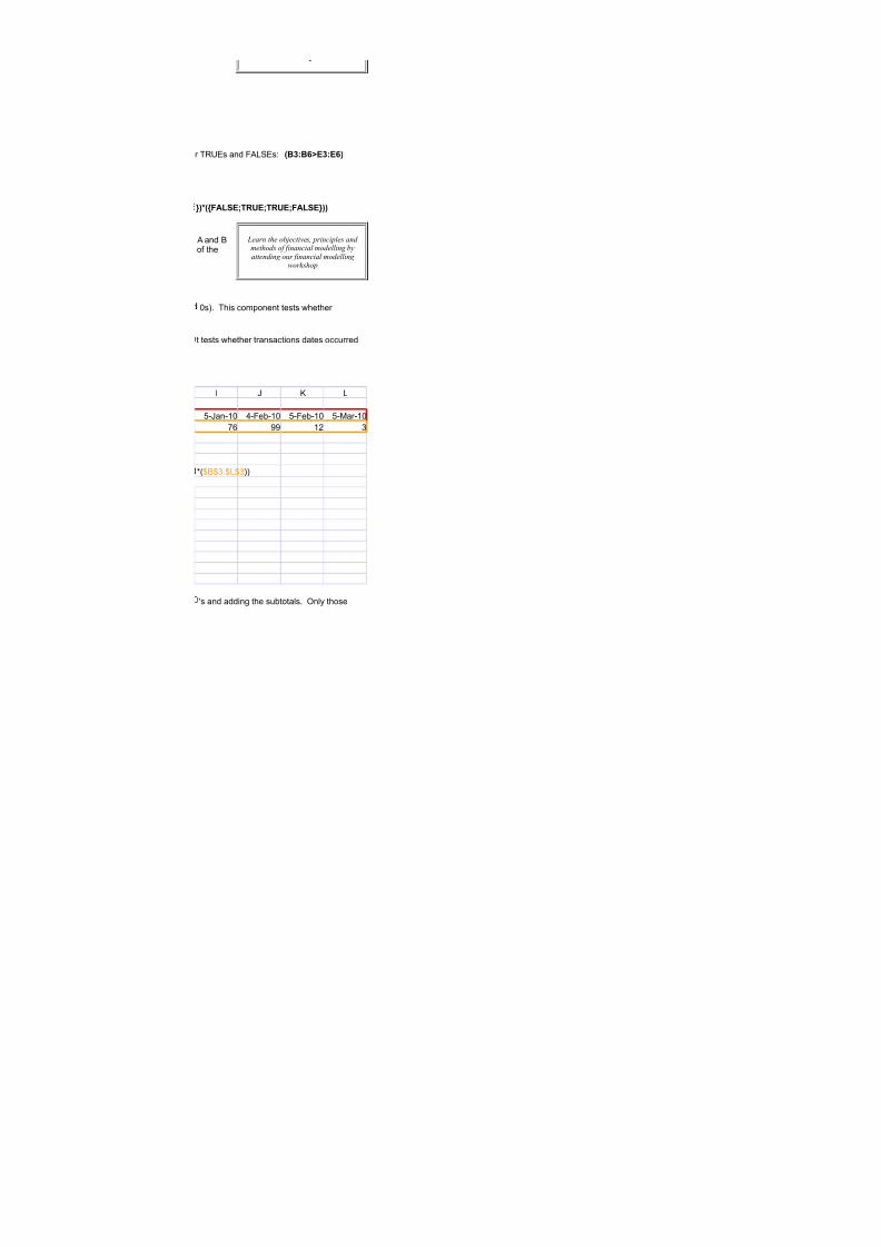
7/18/2019 SpreadsheetGuide_1.02 (1) - copia
http://slidepdf.com/reader/full/spreadsheetguide102-1-copia 88/114
I J H ,
@-Jan-%" 9-1eb-%" @-1eb-%" @-6ar-%"
A ** %) !
r TEG7s and 1,47s: 9,3:,G.3:.;
J;<9H#A(S.I?/8.I?/8.I#A(S.J;;
and &of the
"earn the ob#ectives$ principles andmethods of financial modelling by
attending our financial modellingworkshop
"s(. This component tests whether
t tests whether transactions dates occurred
/P&P!:P,P!((
's and adding the subtotals. 2nly those

7/18/2019 SpreadsheetGuide_1.02 (1) - copia
http://slidepdf.com/reader/full/spreadsheetguide102-1-copia 89/114
&ack to top
ation click hereS
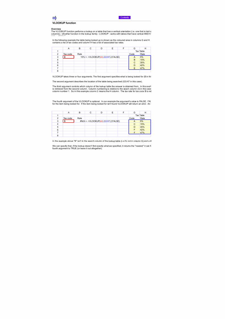
7/18/2019 SpreadsheetGuide_1.02 (1) - copia
http://slidepdf.com/reader/full/spreadsheetguide102-1-copia 90/114
(8+ function
& C 0 7 1 + =
% Tax Table
) Tax code Eate Code Eate
! & %@# @#
9 & %@#
@ C !@#
0 9)#A 7 9A#
8
& C 0 7 1 + =
% Tax Table
) Tax code Eate Code Eate
! & KF @#
9 C %@#
@ 0 !@#
7 9)#
A 1 9A#8
vervie!The D,22HG$ function performs a lookup on a table that has a vertical orientation i.e. one that is laid ocolumns(. Rnother function in the lookup family - ,22HG$ - works with tables that have vertical F0 h
In the following example the table being looked up is shown as the coloured area in columns + and =.contains a list of tax codes and column = has a list of associated tax rates.
L- OD,22HG$ !+!:=A)1,47(
D,22HG$ takes three or four arguments. The first argument specifies what is being looked for & in thi
The second argument describes the location of the table being searched +!:=A in this case(.
The third argument controls which column of the lookup table the answer is obtained from. In this exais retrieved from the second column. Column numbering is relative to the seach column + in this casecolumn number %. 4o in this example column ) means the = column. The tax rate for tax code & is ret
The fourth argument of the D,22HG$ is optional. In our example the argument's value is 1,47. 1for the item being looked for. If the item being looked for isn't found D,22HG$ will return an error. n
L- OD,22HG$ !+!:=A)1,47(
In the example above & isn't in the search column of the lookup table i.e it's not in column +( and a K
;e can specify that if the lookup doesn't find exactly what we specified it returns the nearest it can fifourth argument to TEG7 or leave it out altogether(.

7/18/2019 SpreadsheetGuide_1.02 (1) - copia
http://slidepdf.com/reader/full/spreadsheetguide102-1-copia 91/114
& C 0 7 1 + =
% Tax Table
) Tax code Eate Code Eate
! C @# @#
9 0 %@#
@ 7 !@#
1 9)#A + 9A#
8
L- OD,22HG$ !+!:=A)TEG7(
In the example above the item being looked for - C - doesn't exist in the lookup table. D,22HG$ returthe nearest the lookup finds to C. ;hy does the D,22HG$ choose 's tax rate rather than 0's< ftehow D,22HG$'s searching works:
D,22HG$ assumes the search column is sorted in increasing order. D,22HG$ starts at the top of thecolumn until it finds the first item that is greater than or e5ual to( the item being searched for. In this ecolumn till it hits 0. It then realises it has gone too far and backs up one row. It arrives on the rowreturns.

7/18/2019 SpreadsheetGuide_1.02 (1) - copia
http://slidepdf.com/reader/full/spreadsheetguide102-1-copia 92/114
& C 0 7 1 + =
% Tax Table
) Tax code Eate Code Eate
! C @# @#
9 L- 9 0 %@#
@ 7 !@#
1 9)#
A + 9A#
8
& C 0 7 1 + =
% Tax Table
) Tax code Eate Code Eate
! D %@# @#9 C %@#
@ ; !@#
3 9)#
A > 9A#
8
& C 0 7 1 + =
% Tax Table
) Income Eate Income Eate! @9""" %@# %"""" "#
9 !"""" %@#
@ @@""" !@#
*@""" 9)#
A %@"""" 9A#
8
& C 0 7 1 + =
% Tax Table
) Income Eate Income Eate
! %@9""" 9A# %"""" "#
9 !"""" %@#
@ @@""" !@#
*@""" 9)#
L- OD,22HG$ !+!:=A)TEG7(
similar but more extreme example is the following: ;e want a nearest match for D. 7ven though Dit is C's tax rate that is returned. s in the preceding example D,22HG$ steps through the search coand backs up by one row and returns C's tax rate.
L- OD,22HG$ !+!:=A)TEG7(
This searching behaviour also happens if the search column contains numbers. In the following exampincome levels( in the first search column.
L- OD,22HG$ !+!:=A)TEG7(
In the example above we're looking for the tax rate for an income level of P@9""". Fote that the rate rall income levels between P!"""" and up to but not including( P@@""".
If a nearest match lookup is being done and the item being searched for is larger than the last item in
returned. s in the following example.
L- OD,22HG$ !+!:=A)TEG7(

7/18/2019 SpreadsheetGuide_1.02 (1) - copia
http://slidepdf.com/reader/full/spreadsheetguide102-1-copia 93/114
A %@"""" 9A#
8
=ere the income - P%@9""" - is greater than the last income in the search column - P%@"""". 4o the t
& C 0 7 1 + =
% Tax Table
) Tax code Eate Code Eate
! D !@# @#
9 C %@#
@ D !@#
3 9)#
A > 9A#
8
In a D,22HG$ if we specify a nearest lookup by omitting the fourth argument or having it TEG7( anitem is returned. s in the following example: n exact match for D is found.
L- OD,22HG$ !+!:=A)TEG7(
1or a nearest lookup to work the search column has to be in sorted ascending order. If it is not then tConsider the following example. The search column isn't in sorted order C appears before (. Thelookup expects the search column to be sorted in ascending order. The first item it sees is C. It's looand returns an error.
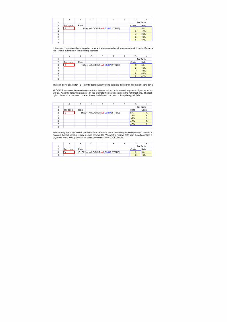
7/18/2019 SpreadsheetGuide_1.02 (1) - copia
http://slidepdf.com/reader/full/spreadsheetguide102-1-copia 94/114
& C 0 7 1 + =
% Tax Table
) Tax code Eate Code Eate
! & %@# C @#
9 %@#
@ 0 !@# 7 9)#
A 1 9A#
8
& C 0 7 1 + =
% Tax Table
) Tax code Eate Code Eate
! & %@# C @#
9 & %@#
@ 0 !@#
7 9)#
A 1 9A#
8
The item being search for - & - is in the table but isn't found because the search column isn't sorted in a
& C 0 7 1 + =
% Tax Table
) Tax code Eate Eate Code
! & KF @#
9 %@# &
@ !@# C
9)# 0
A 9A# 7
8
& C 0 7 1 + =
% Tax Table
) Tax code Eate Code Eate
! D 7rr:@") @#
9 C %@#
L- OD,22HG$ !+!:=A)TEG7(
If the searching column is not in sorted order and we are searching for a nearest match - even if an exafail. That is illustrated in the following scenario.
L- OD,22HG$ !+!:=A)TEG7(
D,22HG$ assumes the search column is the leftmost column in its second argument. If you try to havwill fail. s in the following example. In this example the search column is the rightmost one. The lookright column to be the search one so it uses the leftmost one. nd not surprisingly - it fails.
L- OD,22HG$ !+!:=A)TEG7(
nother way that a D,22HG$ can fail is if the reference to the table being looked up doesn't contain eexample the lookup table is only a single column +(. ;e want to retrieve data from the adacent = -argument to the lookup doesn't contain that column - the D,22HG$ fails.
L- OD,22HG$ !+!:+A)TEG7(
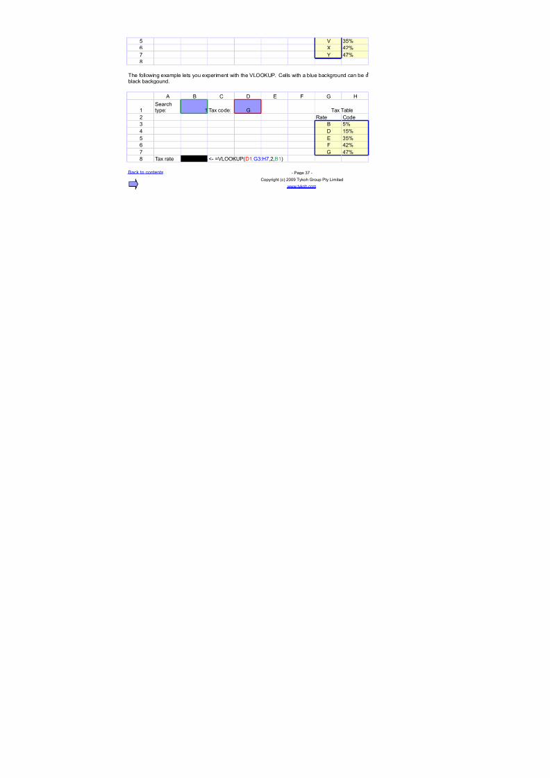
7/18/2019 SpreadsheetGuide_1.02 (1) - copia
http://slidepdf.com/reader/full/spreadsheetguide102-1-copia 95/114
@ D !@#
3 9)#
A > 9A#
8
& C 0 7 1 + =
% % Tax code: + Tax Table
) Eate Code
! & @#
9 0 %@#
@ 7 !@#
1 9)#
A + 9A#
8 Tax rate 9A#
&ack to contents - $age !A -
Copyright c( )""* Tykoh +roup $ty ,imited
www.tykoh.com
The following example lets you experiment with the D,22HG$. Cells with a blue background can be c
black backgound.
4earchtype:
L- OD,22HG$0%+!:=A)&%(

7/18/2019 SpreadsheetGuide_1.02 (1) - copia
http://slidepdf.com/reader/full/spreadsheetguide102-1-copia 96/114
We can provide a mix of classroom$
internet and self learning teaching
ut inriNontal
Column +
s example - in cell !(.
ple the third argument is ). 4o the answer(. The search column is treated as beingrieved and found to be %@#.
47 tells D,22HG$ to find an exact matchexample of this is shown next.
"earn how to choose the best function to solve a problem when several functions
are available by attending one of ourworkshops
F error is returned.
nd rather than an error. To do that we set the

7/18/2019 SpreadsheetGuide_1.02 (1) - copia
http://slidepdf.com/reader/full/spreadsheetguide102-1-copia 97/114
s a rate of @# - which is 's tax rate. isall 0 is closer to C than is . This is
search column and scans down through thatample D,22HG$ will step down the searchwith . nd 's tax rate is what D,22HG$

7/18/2019 SpreadsheetGuide_1.02 (1) - copia
http://slidepdf.com/reader/full/spreadsheetguide102-1-copia 98/114
'eedback from our ,preadsheet skillscourse) %Excellent knowledge and clear
communication from the presenter%
is alphabetically closer to ; than it is to C -lumn till it realises it has gone too far at ;(
le the tax rate table contains numbers
turned is %@#. This rate will be returned for
the search column then the last entry is

7/18/2019 SpreadsheetGuide_1.02 (1) - copia
http://slidepdf.com/reader/full/spreadsheetguide102-1-copia 99/114
ax rate for P%@"""" is returned.
an exact match is found then the exact
We can customise the content of thisinteractive book for particular
audiences
e results will be unpredictable or wrong.lookup fails. The reason it fails is that theing for & and so gives up straight away

7/18/2019 SpreadsheetGuide_1.02 (1) - copia
http://slidepdf.com/reader/full/spreadsheetguide102-1-copia 100/114
scending order.
ct match exists - then the lookup may still
e the search column elsewhere the lookupup has no way of knowing that you intend the
ough columns. Fote that in the followingate( column. &ut since the second

7/18/2019 SpreadsheetGuide_1.02 (1) - copia
http://slidepdf.com/reader/full/spreadsheetguide102-1-copia 101/114
&ack to top
anged. The output is the cell with the
We can provide a mix of classroom$internet and self learning teaching
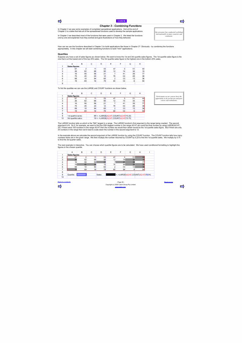
7/18/2019 SpreadsheetGuide_1.02 (1) - copia
http://slidepdf.com/reader/full/spreadsheetguide102-1-copia 102/114
Chapter 3 - Combining Functions
Luartiles
& C 0 7 1 + =
% Sales figures
) A ) %% @! 9A ! @% 99
! ) 8) 8 *" %) A9 !9 %*9 % @ @ )% A 9% !* AA
@ A" 9@ )9 %) A 9 )8 !8
* %" *9 " ) *! %! !
A %* * % A* @ *9 *9
8
To fnd the 5uartiles we can use the ,E+7 and C2GFT functions as shown below.
& C 0 7 1 + =
% Sales figures
) A ) %% @! 9A ! @% 99
! ) 8) 8 *" %) A9 !9 %*
9 % @ @ )% A 9% !* AA
@ A" 9@ )9 %) A 9 )8 !8 * %" *9 " ) *! %! !
A %* * % A* @ *9 *9
8
* %st 5uartile sales: *
%" !rd 5uartile sales: %*
& C 0 7 1 + = I
% Sales figures
) A ) %% @! 9A ! @% 99
! ) 8) 8 *" %) A9 !9 %*
9 % @ @ )% A 9% !* AA
@ A" 9@ )9 %) A 9 )8 !8
* %" *9 " ) *! %! !
A %* * % A* @ *9 *9
8
* Buartile: ! 4ales: %*
%"
&ack to contents - $age !8 - &ack to top
Copyright c( )""* Tykoh +roup $ty ,imited
www.tykoh.com
In Chapter ) we saw some examples of completed spreadsheet applications. nd at the end ofChapter ) is a table that lists all of the spreadsheet functions used to develop the sample applications.
In Chapter ! we described most of the functions that were used in Chapter ). ;e listed the functionsone by one and explained how they worked and gave illustrations of how they behaved.
Our presenter has conducted workshopsinternationally in many countries and
continents
=ow can we use the functions described in Chapter ! to build applications like those in Chapter )< 2bviously - by combining the functionsappropriately. In this chapter we will start combining functions to build mini applications.
4uppose you have a set of sales figures as shown below. ;e want to know the %st and !rd 5uartile sales figures. The %st 5uartile sales figure is theone that is at the lowest end of the top )@# sales. The !rd 5uartile sales figure is the highest one in the bottom )@# sales.
2articipants on our courses have theopportunity to do on!line pre and post!
course self!evaluations
L- O,E+7 ):=AC2GFT ):=A(/".)@(
L- O,E+7 ):=AC2GFT ):=A(/".A@(
The ,E+7 function tells us which is the Fth largest in a range. The ,E+7 function's first argument is the range being counted. The secondargument is F. 4o if for example we want to find the )@th biggest number in the range ):=A we could find that number by using ,E+7):=A)@(. If there were %"" numbers in the range ):=A then the number we would then obtain would be the %st 5uartile sales figure. &ut if there are only)@ numbers in the range then we'd need to scale down the number in the second argument to %).
In the example above we calculate the second argument of the ,E+7 function by using the C2GFT function. The C2GFT function tells how manynumbers there are in the given range. ;e then multiply the number returned by C2GFT by ".)@ to find the %st 5uartile sales. ;e multiply by ".A@to find the !rd 5uarter sales.
The next example in interactive. >ou can choose which 5uartile figures are to be calculated. ;e have used conditional formatting to highlight thefigures in the chosen 5uartile.
L- O,E+7 ):=AC2GFT ):=A(/&*9(

7/18/2019 SpreadsheetGuide_1.02 (1) - copia
http://slidepdf.com/reader/full/spreadsheetguide102-1-copia 103/114
Complex counting
& C 0 7 1 + = I
% Count number of codes starting with: C
)
! Fumber codes starting with C: %
9
@ Codes
1)!9A +%)!8 79!@* "%%
%" 1%)"%% +)!"%) C%%%
%! &"%)
& C 0 7 1 + =% Count number of codes starting with C
)
! Fumber codes starting with C: %
9
@ Codes
1)!9 " % L- TEG7
A +%)! " L- O,71TA%(OP7P% L- TEG7
8 79!@ " L- O,71T8%(OP7P% L- TEG7
* "%% " L- O,71T*%(OP7P% L- TEG7
%" 1%)" " L- O,71T%"%(OP7P% L- TEG7
%% +)!" " L- O,71T%%%(OP7P% L- TEG7
%) C%%% % L- O,71T%)%(OP7P% L- TEG7
%! &"%) " L- O,71T%!%(OP7P% L- TEG7
&ack to contents - $age !* - &ack to top
Copyright c( )""* Tykoh +roup $ty ,imited
www.tykoh.com
Our financial modelling course coversthe finance and accounting concepts that
underlay financial modelling
=ere we look at an illustration of how 4G6$E20GCT can be used in complex conditional counting. &yconditional counting we mean counting only when a certain criterion is satisfied.
The example below contains a list of product codes in column in cells :%!. ;e want to find the number ofproduct codes starting with a particular letter. That letter is specified by the user i.e. you( in cell 7%.
L- O4G6$E20GCT,71T :%!(OP7P%(/%(
In this example we use the ,71T function to get the leftmost character of each product code in :%!. ;e then use the 4G6$E20GCT functionto find the number of times the left character e5uals the character we want to count. ;e need to use a trick with 4G6$E20GCT. ;e multiply by% because 4G6$E20GCT needs to have at least two things to multiply together.
R1or more information about the 4G6$E20GCT function click hereS
If you find the example above a bit difficult to follow - and it is fairly complex - then look at the example below. It solves the same problem in muchthe same way as above but uses extra spreadsheet cells for intermediate calculations. Fote the dummy column of TEG7s in column +. Theseare needed because the 4G6$E20GCT needs at least two arguments to multiply together.
Attend one of our workshops and learnhow to use a wide range of spreadsheet functions in practical finance settingsL- O4G6$E20GCT&:&%!/1:1%!(
L- O,71T %(OP7P%
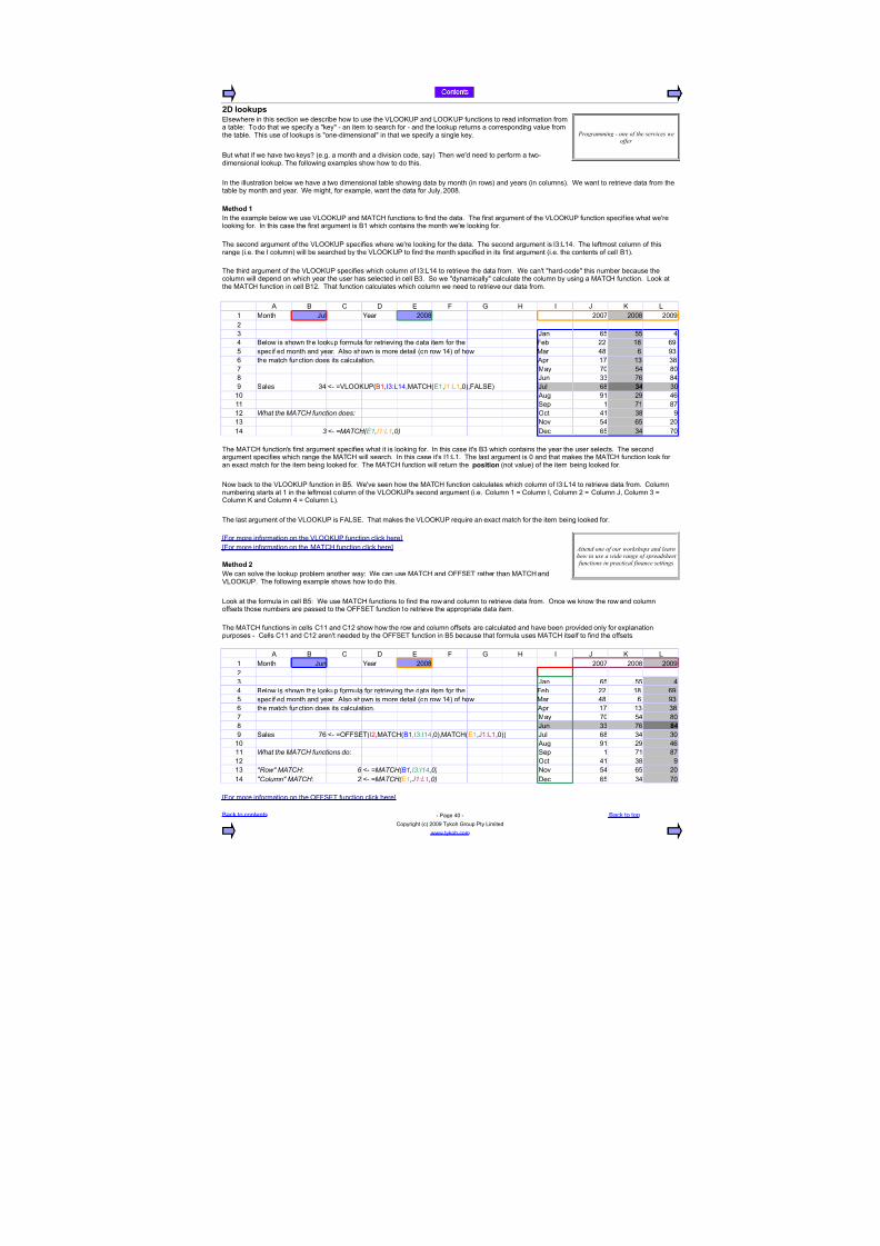
7/18/2019 SpreadsheetGuide_1.02 (1) - copia
http://slidepdf.com/reader/full/spreadsheetguide102-1-copia 104/114
2- lookups
Method 1
& C 0 7 1 + = I J H ,
% 6onth Jul >ear )""8 )""A )""8 )""*
)
! Jan @ @@ 9
9 &elow is shown the lookup formula for retrieving the data item for the 1eb )) %8 *
@ specified month and year. lso shown is more detail on row %9( of how 6ar 98 *!
the match function does its calculation. pr %A %! !8
A 6ay A" @9 8"
8 Jun !! A 89
* 4ales !9 Jul 8 34 !"%" ug *% )* 9
%% 4ep % A% 8A
%) hat the 5-CE function does: 2ct 9% !8 *
%! Fov @9 @ )"
%9 < 0ec @ !9 A"
The last argument of the D,22HG$ is 1,47. That makes the D,22HG$ re5uire an exact match for the item being looked for.
Method 2
& C 0 7 1 + = I J H ,
% 6onth Jun >ear )""8 )""A )""8 )""*
)
! Jan @ @@ 9
9 &elow is shown the lookup formula for retrieving the data item for the 1eb )) %8 *
@ specified month and year. lso shown is more detail on row %9( of how 6ar 98 *!
the match function does its calculation. pr %A %! !8
A 6ay A" @9 8"
8 Jun !! A )4
* 4ales A Jul 8 !9 !"
%" ug *% )* 9
%% hat the 5-CE functions do: 4ep % A% 8A
7lsewhere in this section we describe how to use the D,22HG$ and ,22HG$ functions to read information from
a table: To do that we specify a key - an item to search for - and the lookup returns a corresponding value fromthe table. This use of lookups is one-dimensional in that we specify a single key. 2rogramming ! one of the services weoffer
&ut what if we have two keys< e.g. a month and a division code say( Then we'd need to perform a two-dimensional lookup. The following examples show how to do this.
In the illustration below we have a two dimensional table showing data by month in rows( and years in columns(. ;e want to retrieve data from thetable by month and year. ;e might for example want the data for July )""8.
In the example below we use D,22HG$ and 6TC= functions to find the data. The first argument of the D,22HG$ function specif ies what we'relooking for. In this case the first argument is &% which contains the month we're looking for.
The second argument of the D,22HG$ specifies where we're looking for the data. The second argument is I!:,%9. The leftmost column of thisrange i.e. the I column( will be searched by the D,22HG$ to find the month specified in its first argument i.e. the contents of cell &%(.
The third argument of the D,22HG$ specifies which column of I!:,%9 to retrieve the data from. ;e can't hard-code this number because thecolumn will depend on which year the user has selected in cell &!. 4o we dynamically calculate the column by using a 6TC= function. ,ook atthe 6TC= function in cell &%). That function calculates which column we need to retrieve our data from.
L- OD,22HG$&%I!:,%96TC=7%I%:,%"(1,47(
FB G5-CE% ;1+1:$10'
The 6TC= function's first argument specifies what it is looking for. In this case it's &! which contains the year the user selects. The secondargument specifies which range the 6TC= will search. In this case it's I%:,%. The last argument is " and that makes the 6TC= function look foran exact match for the item being looked for. The 6TC= function will return the position not value( of the item being looked for.
Fow back to the D,22HG$ function in &@. ;e've seen how the 6TC= function calculates which column of I!:,%9 to retrieve data from. Columnnumbering starts at % in the leftmost column of the D,22HG$s second argument i.e. Column % O Column I Column ) O Column J Column ! OColumn H and Column 9 O Column ,(.
R1or more information on the D,22HG$ function click hereS
Attend one of our workshops and learnhow to use a wide range of spreadsheet functions in practical finance settings
R1or more information on the 6TC= function click hereS
;e can solve the lookup problem another way: ;e can use 6TC= and 21147T rather than 6TC= andD,22HG$. The following example shows how to do this.
,ook at the formula in cell &@: ;e use 6TC= functions to find the row and column to retrieve data from. 2nce we know the row and columnoffsets those numbers are passed to the 21147T function to retrieve the appropriate data item.
The 6TC= functions in cells C%% and C%) show how the row and column offsets are calculated and have been provided only for explanationpurposes - Cells C%% and C%) aren't needed by the 21147T function in &@ because that formula uses 6TC= itself to find the offsets.
L- O21147TI)6TC=&%I!:I%9"(6TC=7%J%:,%"((

7/18/2019 SpreadsheetGuide_1.02 (1) - copia
http://slidepdf.com/reader/full/spreadsheetguide102-1-copia 105/114
Applications of the MAD and M$ functions
-etecting duplicates
& C 0 7 1 +% --- Transactions ---
) Code -mount
! &TE%) )A %
9 &TE%! !) % L- OC2GFTI1PP!:PPA9(
@ C1"* * % L- OC2GFTI1PP!:PPA@(
01%) 8 % L- OC2GFTI1PP!:PPA(
A &0% 9 % L- OC2GFTI1PP!:PPAA(
8
* 6ax fre5uency %
%"
%% 0uplicates: Fo
%)
The example above is interactive. >ou can set the transaction code in cell to be either a duplicate of another or not to duplicate another.
+a'back period
2n row A we calculate the cumulative cash flows.
& C 0 7 1 + = I J
%
) >ear: )""@ )"" )""A )""8 )""* )"%"
!
9 Cash flow: -!) - %@ )" )! 9@@
A Cumulative cash flow: -)@ -!% -% 9 )A A)
8
* F F F )""8 )""* )"%"
%"%%
%) $ayback year: )""8
%!
The example above is interactive. >ou can change the cash flow in cell 09 to alter the payback year.
&ack to contents - $age 9% - &ack to top
Copyright c( )""* Tykoh +roup $ty ,imited
www.tykoh.com
.onsulting on spreadsheet$ modellingand &uantitative issues ! a service we
offer
In this section we look at applications of the 63 and 6IF functions to problems that re5uire other functions alsoto be used.
RTo revise basics about the 63 and 6IF functions click here.S
In the following example we want to test whether transaction codes in a list of transaction codes are duplicated.The transaction codes are in cells !:A below.
C2GFTI1 functions in cells 0!:0A count the number of times each transaction code occurs. If a transaction code occurs more than once thatmeans it has been duplicated.
The 63 function in cell C)9 finds the maximum of the number of occurrences of each transaction code. If the maximum is more than one thenthat means one or more transaction codes are duplicated. The I1 function in cell C%% reports the result of the duplication test. That cell shows >esor Fo depending on whether duplication has been found or not.
Attend one of our workshops and learnhow to use a wide range of spreadsheet functions in practical finance settings
1re5uency oftransactions
L- OC2GFTI1PP!:PPA !(
L- O630!:0A(
L- OI1C*M%>esFo(
In the example below we determine the payback period on a proect. ;e track the proect cash flows. The cash flows are initially negative and thenbecome positive. ;e find the date at which the first cumulative cash flow becomes positive.
Eow 9 below contains the proect cash flows. They are initially negative i.e. cash outgoings - investments( and later become positive i.e. cashincomings - return on investment(.
L- O+AQ=9
Cumulative cash flowis Qve:
L- OI1=AM"=)F(
L- O6IFC*:=*(
2n row * we check whether the cumulative cash flow is greater than Nero. If it is then we remember the year in which that occurred. If the cashflow is not greater than Nero we indicate that with an F.
,ast we use a 6IF function in cell C%) to find the smallest i.e. first( year in row *. Fote that 6IF ignores the Fs rather than interpreting them asNero - for if 6IF had treated F as Nero the payback year would have been calculated as Nero.
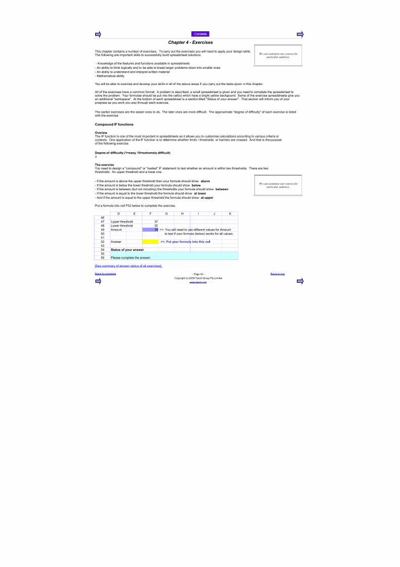
7/18/2019 SpreadsheetGuide_1.02 (1) - copia
http://slidepdf.com/reader/full/spreadsheetguide102-1-copia 106/114
Chapter 4 - Exercises
- Hnowledge of the features and functions available in spreadsheets
- n ability to think logically and to be able to break larger problems down into smaller ones
- n ability to understand and interpret written material
- 6athematical ability
>ou will be able to exercise and develop your ski lls in all of the above areas if you carry out the tasks given in this chapter.
Compound $# functions
-egree of difficult' 916eas'= 1*6extremel' difficult;
!
$ut a formula into cell 1@) below to complete the exercise.
0 7 1 + = I J H
9
9A Gpper threshold !A
98 ,ower threshold !@
9* mount !8 LL- >ou will need to use different values for mount
@" to test if your formula below( works for all values.@%
@) nswer KK% +ut 'our formula into this cell
@!
@9 Status of 'our ans!er
@@
$lease complete the answer.@
R4ee summary of answer status of all exercisesS.
&ack to contents - $age 9) - &ack to top
Copyright c( )""* Tykoh +roup $ty ,imited
www.tykoh.com
We can customise our courses for particular audience
This chapter contains a number of exercises. To carry out the exercises you will need to apply your design skills.The following are important skills to successfully build spreadsheet solutions:
ll of the exercises have a common format: problem is described a small spreadsheet is given and you need to complete the spreadsheet tosolve the problem. >our formulae should be put into the cells( which have a bright yellow backgound. 4ome of the exercise spreadsheets give youan additional workspace. t the bottom of each spreadsheet is a section titled 4tatus of your answer. That section will inform you of yourprogress as you work you way through each exercise.
The earlier exercises are the easier ones to do. The later ones are more difficult. The approximate degree of difficulty of each exercise is listedwith the exercise.
verie!The I1 function is one of the most important in spreadsheets as it allows you to customise calculations according to various criteria orcontexts. 2ne application of the I1 function is to determine whether limits thresholds or barriers are crossed. nd that is the purposeof the following exercise.
?he exercise>ou need to design a compound or nested I1 statement to test whether an amount is within two thresholds. There are twothresholds: n upper threshold and a lower one.
We can customise our courses for particular audience
- If the amount is above the upper threshold then your formula should show above
- If the amount is below the lower theshold your formula should show belo!- If the amount is between but not including( the thresholds your formula should show bet!een
- If the amount is e5ual to the lower threshold the formula should show at lo!er
- nd if the amount is e5ual to the upper threshold the formula should show at upper

7/18/2019 SpreadsheetGuide_1.02 (1) - copia
http://slidepdf.com/reader/full/spreadsheetguide102-1-copia 107/114
Conditional counting
vervie!
-egree of difficult' 916eas'= 1*6extremel' difficult;
@
?he exercise
0 7 1 + = I J H ,
%A 6onth: 2ct-"* Fov-"* 0ec-"* Jan-%" 1eb-%" 6ar-%"
%8 0ept. $erformance level: & C & 0 C
%*
)" Fumber of times performance was between is K% our ans!er
)% and including( &)) Calculations
)!
)9
)@
)
)A Status of 'our ans!er
)8
$lease complete the answer.)*
!"
R4ee summary of answer status of all exercisesS.
&ack to contents - $age 9! - &ack to top
Copyright c( )""* Tykoh +roup $ty ,imitedwww.tykoh.com
Exercises in our spreadsheet skills andmodelling courses give you instant
feedback of your progressThis exercise involves counting conditionally. The best formulae to use are either 4G6$E20GCT or acombination of C2GFTI1 and I1.
In cell J)" put a formula that gives the number of times the departmental performances were between the levels selected in the blue cells on row)". 1or example if the user selects & and 0 or 0 and &( then the formula should return the number of times performances were &C or 0.

7/18/2019 SpreadsheetGuide_1.02 (1) - copia
http://slidepdf.com/reader/full/spreadsheetguide102-1-copia 108/114
?racking cashflo!s
-egree of difficult' 916eas'= 1*6extremel' difficult;
)
4o if there is insufficient capacity in ccount K% to pay the entire negative cash flow the residual amount must be withdrawn from ccount K).
0 7 1 + = I J H , 6 F!! 1acility limit ccount K% !""""( Calculations
!9 7xtra workspace isn't really re5uired for this 5uestion -
!@ 2pening acc. K% balance %A"""( but here's some anyway.
! 2pening acc. K) balance -!A!8 Cash surplus need( )""""
!*
9" cc. K% deposit withdrawal(
$lease complete the answer.9%
9) cc. K) deposit withdrawal(
$lease complete the answer.9!
99 Closing acc. K% balance
$lease complete the answer.9@
9 Closing acc. K) balance
$lease complete the answer.9A
R4ee summary of answer status of all exercisesS.
&ack to contents - $age 99 - &ack to top
Copyright c( )""* Tykoh +roup $ty ,imited
www.tykoh.com
The exercise below is about finding the siNe and direction of cash flows in two accounts. Tocomplete the exercise you will need to design some formulae to calculate: %( ;hether cash is goinginto or out of accounts )( how the cash flow is split between the accounts and !( the amount
involved.
Our Visual Basic course shows how toincrease the %wow!factor% of your
developed applications
,ook at the spreadsheet below. The spreadsheet keeps track of cash flows and balance in two accounts: ccount K% and account K). &othaccounts can be in credit or debit.
The initial balances in the two accounts are shown in cells +!@ and +!. There is a limit on how much in debit account K% can be. That limit isshown as a negative number( in cell +!!.
Cell +!8 defines a cash flow. The cash flow can be positive i.e. incoming( or it can be negative i.e. going out(. If the cash is coming in then itneeds to be deposited in one or both of ccounts K% and K).
This is a rule that defines what needs to be done with a positive cash flow. The cash flow is first applied to reducing ccount K%'s debit balance. If
the cash flow is greater than the debit balance then only enough is deposited into that account to set the balance to Nero. ny residual amount fromthe cash flow is deposited into ccount K).
4o for example if ccount K% has a debit balance of %A"""( and a cash flow of )"""" occurs then %A""" is deposited into ccount K% and !"""into ccount K). If on the other hand a cash flow of """ occurs then all of that amount is deposited into ccount K%.
This is a rule that defines what needs to be done with a negative cash flow. withdrawal is made from ccount K% e5ual to the amount of the cashflow. =owever ccount K% cannot go into debit to more than the amount shown in cell +!!.
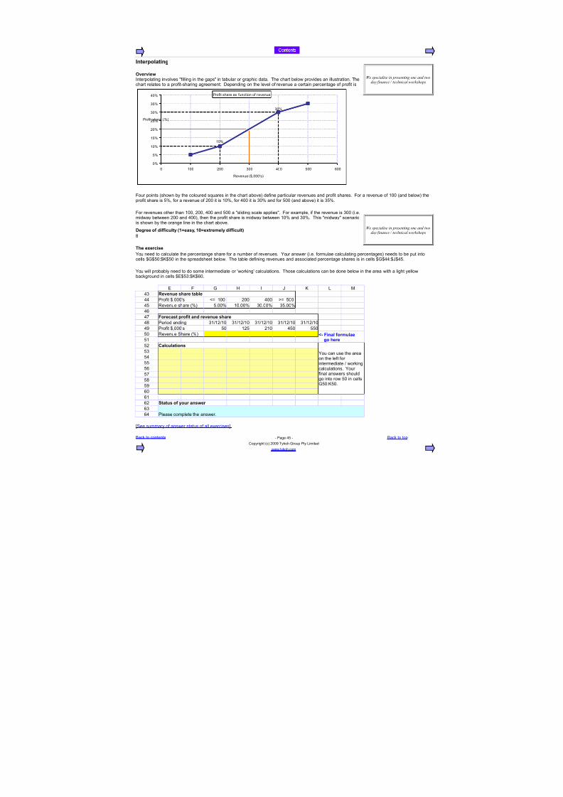
7/18/2019 SpreadsheetGuide_1.02 (1) - copia
http://slidepdf.com/reader/full/spreadsheetguide102-1-copia 109/114
$nterpolating
-egree of difficult' 916eas'= 1*6extremel' difficult;
8
?he exercise
7 1 + = I J H , 6
9! /evenue share table
99 $rofit P"""'s LO %"" )"" 9"" MO @""
9@ Eevenue share #( @.""# %".""# !".""# !@.""#
9
9A #orecast profit and revenue share
98 $eriod ending !%%)%" !%%)%" !%%)%" !%%)%" !%%)%"
9* $rofit P"""'s @" %)@ )%" 9@" @@"@" Eevenue 4hare #(
@%
@) Calculations
@!
@9
@@
@
@A
@8
@*
"
%
) Status of 'our ans!er
!
$lease complete the answer.9
R4ee summary of answer status of all exercisesS.
&ack to contents - $age 9@ - &ack to top
Copyright c( )""* Tykoh +roup $ty ,imited
www.tykoh.com
We specialise in presenting one and two
day finance / technical workshops
vervie!Interpolating involves filling in the gaps in tabular or graphic data. The chart below provides an illustration. Thechart relates to a profit-sharing agreement: 0epending on the level of revenue a certain percentage of profit is
1our points shown by the coloured s5uares in the chart above( define particular revenues and profit shares. 1or a revenue of %"" and below( theprofit share is @# for a revenue of )"" it is %"# for 9"" it is !"# and for @"" and above( it is !@#.
1or revenues other than %"" )"" 9"" and @"" a sliding scale applies. 1or example if the revenue is !"" i.e.midway between )"" and 9""( then the profit share is midway between %"# and !"#. This midway scenariois shown by the orange line in the chart above.
We specialise in presenting one and twoday finance / technical workshops
>ou need to calculate the percentange share for a number of revenues. >our answer i.e. formulae calculating percentages( needs to be put intocells P+P@":PHP@" in the spreadsheet below. The table defining revenues and associated percentage shares is in cells P+P99:PJP9@.
>ou will probably need to do some intermediate or 'working' calculations. Those calculations can be done below in the area with a light yellowbackground in cells P7P@!:PHP".
K% #inal formulae go here
>ou can use the areaon the left forintermediate workingcalculations. >ourfinal answers shouldgo into row @" in cells+@":H@".
" %"" )"" !"" 9"" @"" """#
@#
%"#
%@#
)"#
)@#
!"#
!@#
9"#
%"#
!"#
$rofit share as function of r evenue
Eevenue P"""'s(
$rofit share #(

7/18/2019 SpreadsheetGuide_1.02 (1) - copia
http://slidepdf.com/reader/full/spreadsheetguide102-1-copia 110/114
Complex lookups
-egree of difficult' 916eas'= 1*6extremel' difficult;
%"
?he exercise
0 7 1 + = I J H , 6)) &etween %-Jul-%" +nterruption schedule %inclusive
)! ... and !%-Jan-%" start and end dates'
)9 6tart date ;nd date
)@ K% our ans!er !"-0ec-"* )-Jan-%"
) @-Jan-%" -Jan-%"
)A !%-Jan-%" !%-Jan-%"
)8 )A-1eb-%" )-6ar-%"
)* )-6ay-%" %-Jul-%"
!" Calculations
!%
!)
!!
!9
!@
! Status of 'our ans!er
!A
$lease complete the answer.!8
R4ee summary of answer status of all exercisesS.
&ack to contents - $age 9 - &ack to top
Copyright c( )""* Tykoh +roup $ty ,imited
www.tykoh.com
012V gives a different answer if cellsare blank than when they contain 3ero !
these and other %traps% are explained inour workshops
>ou are modelling the operations of a business. The operations will be impacted by the business's dependenceon a critical resource. That resource is expected to be unavailable over certain periods. Those periods are
described in the Interruption schedule below.
There may be Nero one or more interruption periods in any month. Interruption periods may span month endsand month beginnings. n interruption period may be as short as one day or as long as several months. ninterruption period may already be in effect at the start of the selected month and another or the same( maypersist past the end of that month.
Calculate the number of productive i.e. uninterrupted( days in the selected month. >our answer should work even if the information in theinterruption schedule is changed i.e. you shouldn't hard-code your answer.(
... the number of un-interrupted days is:

7/18/2019 SpreadsheetGuide_1.02 (1) - copia
http://slidepdf.com/reader/full/spreadsheetguide102-1-copia 111/114
Status of .xercises
1ollowing is the completion status of the exercises in this section.
;xercise Degree of difficulty %*' Completion status 4tatus
Compound I1 functions ! Fot attempted )
Conditional counting @ Fot attempted )
Tracking cashflows ) Fot attempted )
Interpolating A Fot attempted )
Complex lookups %" Fot attempted )
/ O 0egree of difficulty on a scale from % to %" - % is easy and %" is very difficult.
&ack to contents - $age 9A - &ack to top
Copyright c( )""* Tykoh +roup $ty ,imited
www.tykoh.com
We specialise in presenting one and two
day finance / technical workshops

7/18/2019 SpreadsheetGuide_1.02 (1) - copia
http://slidepdf.com/reader/full/spreadsheetguide102-1-copia 112/114
Chapter 5 - Next steps
Congratulations on having made it up to here. ;e hope that by now you will have:
- ,ooked at examples of the kinds of things you can do with spreadsheets in Chapter %(- Eeviewed some of the important spreadsheet functions in Chapter )(
-
- ttempted one or more of the exercises listed in Chapter 9.
4o what's next< These are some possibilities:
&ack to contents - $age 98 -
Copyright c( )""* Tykoh +roup $ty ,imited
www.tykoh.com
We can customise the content of thisinteractive book for particular
audiences
4tudied how the building blocks in Chapter ) can be combined to build mini-applicationsin Chapter !(
0o a free on-line self-evaluation of the skills covered in this guide.
Check on-line to see whether a newer and improved version of this guide is available for download.
,ook at workshops we offer that cover in more depth the concepts touched on in this guide.
4ubmit suggestions for improving or feedback about this guide.
&ack to top

7/18/2019 SpreadsheetGuide_1.02 (1) - copia
http://slidepdf.com/reader/full/spreadsheetguide102-1-copia 113/114
ndex &4 ,E+7
)% )*
)*
F0)) ,71T
!"
ggregating !*
!
,7F
ttributing !"
%9
,ogic
D7E+7 ))
)!
!9 ,ooking up
%"
veraging
9 ,22HG$
!%&ook
9 6TC=
!)
Charting
@ 63
!!
C=2247
)9 6I0
)9 !"
Complex 6IF
9 !!
Compound 21147T
)A !9
!9
Concatenation operator !9
) !9
!9
Conditional
9! 2ption
%8
Conditions
)) 2E
KKK
Contents
) Buartile
)*
Contingency %8 EI+=T
KKK
Cross reference
)" E2GF0
%!
C2GFT
)@ $rioritising
%%
C2GFTI1
) Eanking
9! %)
)
4ample applications
Counting !
9! %9!* 9
@
0uplicates A
function function
used to calculate 5uartiles
function
function
used in complex counting
sample application
function
sample application
conditions and tests
function
used with 21147T
sample application
sample application
function
version of
function
sample application
function
function
used for scenarios function
lookups - exercise function
I1 - exercise five argument form
negative arguments
three argument form
used with C2GFTI1 used for scenarios
used with D7E+7
Counting - exercise
valuing
,ogical
function
table of contents
using ,E+7 to calculate
valuing option
function
of functions used
function
function
sample application
with concatenation operator
conditional count exercise sample application
function
aggregating
conditionally - exercise attributingcomplex - using 4G6$E20GCT averaging
charting
filtering

7/18/2019 SpreadsheetGuide_1.02 (1) - copia
http://slidepdf.com/reader/full/spreadsheetguide102-1-copia 114/114
*
7xercise %"
9) %%
9! %)
99 %9
9@ %@9 %
7xercises 4cenario analysis
9A %9)9
1iltering !9
A
4cheduling
1unction %@
)%
)) 4easonalising
)! %
)9
)" 4ensitivity
)@ 8) %A
)A
)8 4orting
)* )*
!"
!" 4tatus
!% 9A
!)
!! 4G6
!" !@
!! !@
!9
)) 4G6$E20GCT
!" !*
%! !
!@ !
!
!A Tests
))
+rouping
! Top
=ighlighting Daluing
8
%9
highlighting highlighting
interpolatinglooking up
on compound I1 prioritisingon conditional counting ranking
on tracking cash flows scenario analysing
on interpolating schedulingon complex lookups seasonalising
status of completed sample applicationusing C=2247
using 21147T
sample application
sample application
&4
F0
D7E+7 sample application
C=2247cross reference
C2GFT to interest ratesC2GFTI1 to value drivers
I1
I4F
,E+7 by using ,E+7 function
,71T
,7F
,22HG$ of exercises completed6TC=
63
6I0 function
6IF differences to addition
21147T
2E
EI+=T used in complex countingE2GF0 function
4G6 grouping by date
4G6$E20GCT
D,22HG$
logical
by date - 4G6$E20GCT
F - highlighting
duplicates
sample application cash flows debt
top F e5uity enterprise


![Copia de Taller_OHSAS_18001[1][1][1]](https://img.pdfslide.us/doc/110x75/577d22371a28ab4e1e96d7f9/copia-de-tallerohsas18001111.jpg)
![Copia de Quimica_1[1]](https://img.pdfslide.us/doc/110x75/577c78911a28abe05490590b/copia-de-quimica11.jpg)


![Detroit Manual Copia[1]](https://img.pdfslide.us/doc/110x75/549dbc27b4795988208b45aa/detroit-manual-copia1.jpg)