SPOUSAL MOBILITY AND EARNINGS* - …spot.colorado.edu/~mckinnis/McKinnishDemography.pdf · migration (Clark and Huang 2006; Cooke 2001, 2003; Jacobsen and Levin 1997). There are still,

Demography, Volume 45-Number 4, November 2008: 829–849 829

I

SPOUSAL MOBILITY AND EARNINGS*

TERRA MCKINNISH

An important fi nding in the literature on migration has been that the earnings of married women typically decrease with a move, while the earnings of married men often increase with a move, sug-gesting that married women are more likely to act as the “trailing spouse.” This article considers a related but largely unexplored question: what is the effect of having an occupation that is associated with frequent migration on the migration decisions of a household and on the earnings of the spouse? Further, how do these effects differ between men and women? The Public Use Microdata Sample from the 2000 U.S. decennial census is used to calculate migration rates by occupation and education. The analysis estimates the effects of these occupational mobility measures on the migration of couples and the earnings of married individuals. I fi nd that migration rates in both the husband’s and wife’s oc-cupations affect the household migration decision, but mobility in the husband’s occupation matters considerably more. For couples in which the husband has a college degree (regardless of the wife’s educational level), a husband’s mobility has a large, signifi cant negative effect on his wife’s earnings, whereas a wife’s mobility has no effect on her husband’s earnings. This negative effect does not exist for college-educated wives married to non-college-educated husbands.

n the substantial literature on the relationship between migration and earnings, an impor-tant fi nding has been that the earnings of married women typically decrease with a move, while the earnings of married men often increase with a move. This is consistent with the notion that married women are more likely to act as the “trailing spouse” or to be a “tied mover.” This article considers a related but largely unexplored question: what is the effect of having an occupation that is associated with frequent migration on the migration deci-sions of a household as well as on the earnings of the spouse? And how do these effects differ between men and women?

There are three reasons to move beyond the previous analysis of household moves to studying the effect of occupational mobility on migration and earnings. First, the analysis of changes in employment and earnings of movers is only part of a broader discovery concerning the extent to which the earnings of husbands and wives are affected by the ability to move to or stay in optimal locations. Second, the existing literature relies on the comparison of movers to nonmovers. Even longitudinal comparisons will not completely eliminate the bias in this comparison because movers likely differ in their earnings growth, not just the level of premigration earnings. Third, the methods used in the literature often do not adequately adjust for occupational differences between men and women, so it is diffi cult to know whether the current fi ndings in the literature are the result of differences in jobs held by men and women, or rather are the result of differences in infl uence on loca-tion decisions. The question pursued in this article is, controlling for an individual’s own occupation and the earnings potential in that occupation, how does the migration rate in a spouse’s occupation affect one’s own labor market outcomes?

This article uses the Public Use Microdata Sample (PUMS) from the 2000 U.S. decen-nial census to calculate mobility measures by occupation and education class. Mobility is measured by the fraction of workers who, in the past fi ve years, have either (a) changed metropolitan area or (b) if in a nonmetropolitan area, changed Public Use Microdata Area (PUMA).1 Using the sample of white, non-Hispanic married couples between the ages of

*Terra McKinnish, Economics Department and Institute of Behavioral Science, University of Colorado, Boulder, CO 80309-0256; e-mail: [email protected]. Helpful comments from Robert Pollak and Ernesto Villanueva, as well as participants at the 2006 ESPE meetings, 2007 ASSA meetings, and 2007 SOLE meetings are gratefully acknowledged.

1. A PUMA is a geographic area, created for census data, of at least 100,000 people that respects state (but not county) boundaries.

830 Demography, Volume 45-Number 4, November 2008

25 and 55 in the 2000 census, I perform migration and earnings analyses separately for four groups of couples: both have college degrees (“power couples”), only the husband has a college degree, only the wife has a college degree; and neither has a college degree.

Results indicate that the mobility rates in both the husband’s and wife’s occupation affect the household migration decision, but mobility in the husband’s occupation matters considerably more. Comparison analysis for never-married individuals indicates that among individuals with college degrees, never-married men and women are equally responsive to occupation mobility in their migration behavior.

The earnings analysis uses occupation fi xed-effects and average wage in occupation-education class to control for substantial heterogeneity in earnings potential. For couples in which the husband has a college degree, the wife’s mobility has no effect on the husband’s earnings, regardless of the wife’s education. However, the husband’s mobility has a large, signifi cant negative effect on the wife’s earnings. This negative effect does not exist for couples in which only the wife has a college degree.

LITERATURE REVIEWEarly work on household migration theorized that a household migrates if the total increase in household income exceeds the total costs of migration. As such, it is possible for a move to reduce one partner’s earnings if the increase in the other partner’s earnings is greater (Mincer 1978; Sandell 1977). Because women have traditionally worked in lower-earning occupations that require less human capital investment, they have historically been less likely to realize large earnings gains or losses from moves. As a result, it stands to reason that location decisions are more often based on the husband’s opportunities, with the wife often acting as a “tied mover” or “tied stayer.”

A number of empirical papers have studied the differential effect of migration on labor market outcomes of wives and husbands (Astrom and Westerlund 2006; Bailey and Cooke 1998; Boyle et al. 1999, 2001, 2002; Clark and Huang 2006; Clark and Withers 2002; Cooke 2001, 2003; Cooke and Bailey 1996; Cooke and Speirs 2005; Jacobsen and Levin 1997; LeClere and McLaughlin 1997; Morrison and Lichter 1988; Nivalainen 2004; Sand-ell 1977; Shauman and Noonan 2007; Shihadeh 1991; Spitze 1984). Most have found that migrating wives experience more negative labor market effects than migrating husbands (for an exception, see Cooke and Bailey 1996). Several studies have found that the negative effects of migration on wives’ employment dissipate within a few years (e.g., Clark and Withers 2002; Spitze 1984). Recent studies have found that the size of the migration effect varies by the mother’s characteristics and migration context. For example, Cooke (2001) found that while nonmothers experience extremely short-lived reductions in employment from migration, the employment impacts of migration are much larger and enduring for married women with children. Bailey and Cooke (1998) found that the nature of immigra-tion matters. Married women experience smaller negative effects from return migration to a previous location, and therefore previously established social networks, than from migra-tion to a new location.

A number of authors (e.g., Bielby and Bielby 1992; Shihadeh 1991) have argued that the symmetry of the neoclassical model of migration—that the household will move for an increase in total income, regardless of whether it is attributable to the husband or wife—does not adequately explain the fi ndings of employment and earnings disruptions for migrating wives. They have argued, instead, that decisions based on traditionally accepted gender roles—in which the husband’s career considerations dominate, regardless of the net change in household income—are more consistent with the empirical evidence.

Several studies have tested whether the husband’s and wife’s expected income gains receive equal weight in the migration decision. Jacobsen and Levin (2000) estimated predicted returns to migration for both the husband and wife. They found that couples are equally responsive to the husband’s and wife’s predicted gain. Rabe (2006) performed a

Spousal Mobility and Earnings 831

similar analysis on British data, incorporating corrections for selection into migration and employment. She also found that couples put equal weight on each partner’s expected wage gain in the migration decision. Jurges (2006) separated German couples into tradi-tional and egalitarian couples, based on the division of housework on Sundays. He found that among the traditional couples, the husband’s education predicts migration, but the wife’s does not. Among egalitarian couples, however, education of both partners factor equally into the migration decision. These studies predominantly support Mincer’s neo-classical model of migration.

A more mixed set of results has emerged from related studies that investigate whether the negative migration effect is reduced for wives with greater earnings potential. Bailey and Cooke (1998) found that the negative migration effect is eliminated for highly educated married women without children. Boyle et al. (1999) categorized couples as male- or female-dominated, based on which member has the higher-status occupation. They found a negative migration effect even for wives in the female-dominated marriages. Cooke (2003) found that even for cases in which the wife contributes a higher fraction of household earnings, migration is typically associated with an earnings increase for men yet no improvement for women. The fact that several studies found that migration harms even wives with high earnings potential suggests that gender roles play a role in household-location decisions.

In the debate between the human capital and gender role models of household migra-tion, the empirical evidence is, therefore, mixed. Although one could say that a particular set of results is more consistent with one model or the other, empirical challenges make it diffi cult to argue that any particular study defi nitively rejects either model. Studies of the effect of migration on the labor market outcomes of husbands and wives face several em-pirical diffi culties. The most fundamental issue is that migrants differ from nonmigrants in ways that make the cross-sectional comparison of migrants and nonmigrants problematic. Some studies have used longitudinal data to control for earnings or employment prior to migration (Clark and Huang 2006; Cooke 2001, 2003; Jacobsen and Levin 1997). There are still, however, realistic sources of bias in these studies. For example, if husbands and wives are in different occupations with different career paths and earnings trajectories, a control for premigration earnings will not suffi ciently control for differences in earnings potential. Another concern is that the wife’s employment and earnings prior to migration may refl ect a response to a negative labor market shock to the husband. It is this negative labor market event that induces the migration, but the wife’s exit from the labor force after the move is a response to the rebound in her husband’s income, rather than an effect of the move itself.

The approach taken in this article is quite different from most of the previous litera-ture because the analysis does not estimate the effect of migration on labor market out-comes. Instead, this study asks whether a wife with a given occupation (in other words, controlling for occupation fi xed effects) typically has earnings that are above or below av-erage for her occupation and education level if her husband works in an occupation with a high migration rate. These results are then compared with those estimating the effect of the wife’s occupational migration rate on her husband’s earnings. The analysis in this article, therefore, does not compare migrants with nonmigrants. Instead, it asks whether having a spouse in an occupation with a high mobility rate is advantageous or disadvanta-geous to labor market earnings, with comparisons made within narrowly defi ned occupa-tion and education groups to avoid bias attributable to unobserved differences in earnings potential. This approach, as will be discussed in greater detail later in this article, is still subject to criticism to the extent that choice of occupation is endogenous to household earnings. On the other hand, this approach avoids many of the empirical challenges in the existing literature on migration outcomes.

Duncan and Perrucci (1976) and Shauman and Noonan (2007) also incorporated occupation-specifi c migration rates, estimated from census data, into their analyses. It is, therefore, worthwhile to discuss the similarities between those studies and the current


one. Duncan and Perrucci (1976), using a small sample of white, married, female college graduates in the 1960s, estimated the effect of occupation-specifi c migration rates on the probability that a couple will migrate. They found that the husband’s occupation migration rate has a positive effect, and that the wife’s occupation migration rate has a negative effect, on the probability that the couple migrates. (This analysis is similar to that performed in Table 4 of the current study.) Shauman and Noonan (2007) used the Panel Study of Income Dynamics to estimate the effects of migration on employment or earnings, allowing the effect of migration to vary by gender. They found that adding controls for occupation-specifi c characteristics, such as the occupation-specifi c migration rate, does not reduce the differentially negative effect of migration on the employment and earnings of wives. Unlike the current study, their study did not consider the effect of spouse’s occupational characteristics on own earnings.

The studies discussed in this review typically included linear controls for educational attainment, but they did not allow the effects of migration to vary by education. There is evidence, however, of a substantially different relationship between migration and employ-ment for workers with high levels of education than for those with low education. Highly educated workers are more likely to move as a form of career advancement, tending to move with a job in hand. Workers with lower education levels tend to move in response to a negative shock to their local labor market, moving to a better labor market to search for a job (Basker 2003). This suggests that the relationship between migration and labor market outcomes for married individuals will likely vary by education level. Unfortunately, much of the previous literature does not allow for this possibility.

The analysis in this article separates couples based on educational attainment. The pri-mary focus is on workers with college degrees—those for whom location choices are more likely important for career advancement. Another set of studies has focused on the loca-tion decisions of “power couples” (couples in which both spouses have a college degree). Costa and Kahn (2000) argued that power couples have increasingly located in urban areas because of the increased prevalence of dual-career households and the resulting co- location problem. Compton and Pollak (2007) performed analysis that strongly suggests that the urban concentration noted by Costa and Kahn results from the attractiveness of urban areas to highly educated individuals and from fact that they match and marry at higher rates in urban areas, rather than because they relocate to urban areas as power couples. Interestingly, Compton and Pollak found that only the education of the husband matters in the location decision. Irrespective of wife’s education, couples in which the husband has a college degree disproportionately locate in larger urban areas. Like Compton and Pollak, I fi nd the results for power couples to be very similar to couples in which only the husband has a college degree.

DATAOccupation Characteristics

The data used in this article are the Public Use Microdata Sample (PUMS) from the 2000 decennial census. Workers are classifi ed into occupation and education classes using the 504 civilian occupation categories in the 2000 census and 8 education classifi cations: less than 9th grade, some high school, high school diploma, some college, bachelor’s degree, master’s degree, professional degree, and doctoral degree.

Two samples are used to generate the data for analysis. The fi rst sample is used to calculate the migration rates and average wages by occupation-education class. These are calculated using the sample of all workers ages 25–55; who resided in the United States in 1995; and for whom occupation, education, and migration status are not allocated. The second sample is the regression sample of white, non-Hispanic married couples described in more detail in the next section.


The 2000 PUMS reports state of residence and Public Use Microdata Area (PUMA) of residence in both 1995 and 2000. A PUMA is a geographic area populated with at least 100,000 people that respects state (but not county) boundaries. Within urban areas, it is smaller than a county; in nonmetropolitan areas, it is typically a county or a group of counties. If the PUMA is entirely contained within metropolitan statistical area (MSA) boundaries, the MSA of residence is identifi ed. For this article, a person is a migrant if in the past fi ve years, either (a) changed metropolitan area; or (b) if in a nonmetropolitan area, moved to a different PUMA. This is similar to the migration defi nition used by Shauman and Noonan (2007). The one limitation of this defi nition of migration is that for individuals residing in a PUMA that crosses MSA lines, the data do not identify whether they reside in the metropolitan or nonmetropolitan part of the PUMA. Therefore, one cannot correctly identify their migration status. For this reason, individuals in these PUMAs are excluded from the migration rate calculations.2

Migration rates and average wages are calculated by occupation and education cat-egory, using all workers ages 25–55.3 Table 1 reports the averages of these occupation- and education-specifi c measures for the white, non-Hispanic married couples in the regres-sion sample. Consistent with the migration literature, Table 1 shows that migration rates increase with education. The table also shows that among workers with less than a college degree, women and men are in occupations with similar migration rates. Among workers

2. I could simply label these individuals as “nonmetropolitan” and determine whether they had changed PUMA. However, this would mistakenly classify many residential moves within a metropolitan area as a migra-tion. Alternatively, treating all individuals in these PUMAs as metropolitan-area residents would require extensive hand-coding of the data using census maps because there is no link in the PUMS data between these PUMA codes and the MSA with which they overlap. Additional analysis was performed using a state-based defi nition of migra-tion, which avoids this loss of sample. The results were quite similar to those presented here, thus making fairly certain that this reduction in sample has little effect on the results.

3. The wage measure is calculated by dividing earnings in 1999 by hours worked in 1999. Hours worked is obtained by multiplying the reported average hours per week by the total weeks worked in 1999. Average wages are computed only among those workers with hourly wages between $3 and $300.

Table 1. Average Occupational Characteristics, by Education Level Occupation- and Education- Average Wage in

Correlation Between Specifi c Migration Rate Occupation-Education Migration Rate and _________________________ _____________________

Education Category Men Women Men Women Average Wage

Less Th an High School 0.099 0.100 14.36 12.04 –0.114 (0.024) (0.027) (2.66) (2.44) High School Diploma 0.110 0.109 17.65 14.68 0.137 (0.032) (0.031) (3.84) (3.68) College Degree 0.183 0.173 26.08 21.64 0.156 (0.046) (0.038) (7.54) (5.98) More Th an a College Degree 0.199 0.163 34.03 27.58 0.207 (0.073) (0.069) (11.81) (8.96)

Notes: Numbers in parentheses are standard deviations. Th e sample is non-Hispanic, white, native-born married couples from the 2000 census with both partners ages 25–55, reporting civilian occupations for last job worked in the past fi ve years (excluded if one or both partners was not employed in the past fi ve years). Mobility and wage rates are calculated using all workers ages 25–55 in occupation and education group, using the 504 civilian occupation categories in the 2000 census and eight education categories: no high school, some high school, high school diploma, some college, college degree, master’s degree, professional degree, and doctoral degree. Migration rate is the fraction of workers who, in the past fi ve years, either (1) changed metropolitan area or (2) if in a nonmetropolitan area, changed PUMA. Wage rate is the average wage of workers with wages between $3 and $300 per hour.


with at least a college degree, women are disproportionately in occupations with lower rates of migration.

Table 1 also reports the correlation between the occupation-education–specifi c migra-tion rate and the occupation-education–specifi c wage rate. Among workers with less than a high school diploma, occupations with higher migration rates tend to have lower wages, but the correlation is positive for workers with more education. This indicates differences in migration behavior between high-education and low-education workers, which have been documented in the migration literature. Skilled workers tend to migrate with a job in hand, and unskilled workers tend to migrate from areas with weak labor markets to areas with strong labor markets to search for a job, often after losing a job. Therefore, low-skilled occupations with high migration rates tend to be those occupied by workers who have experienced some sort of job displacement and/or those jobs that are easy to acquire after of a move.

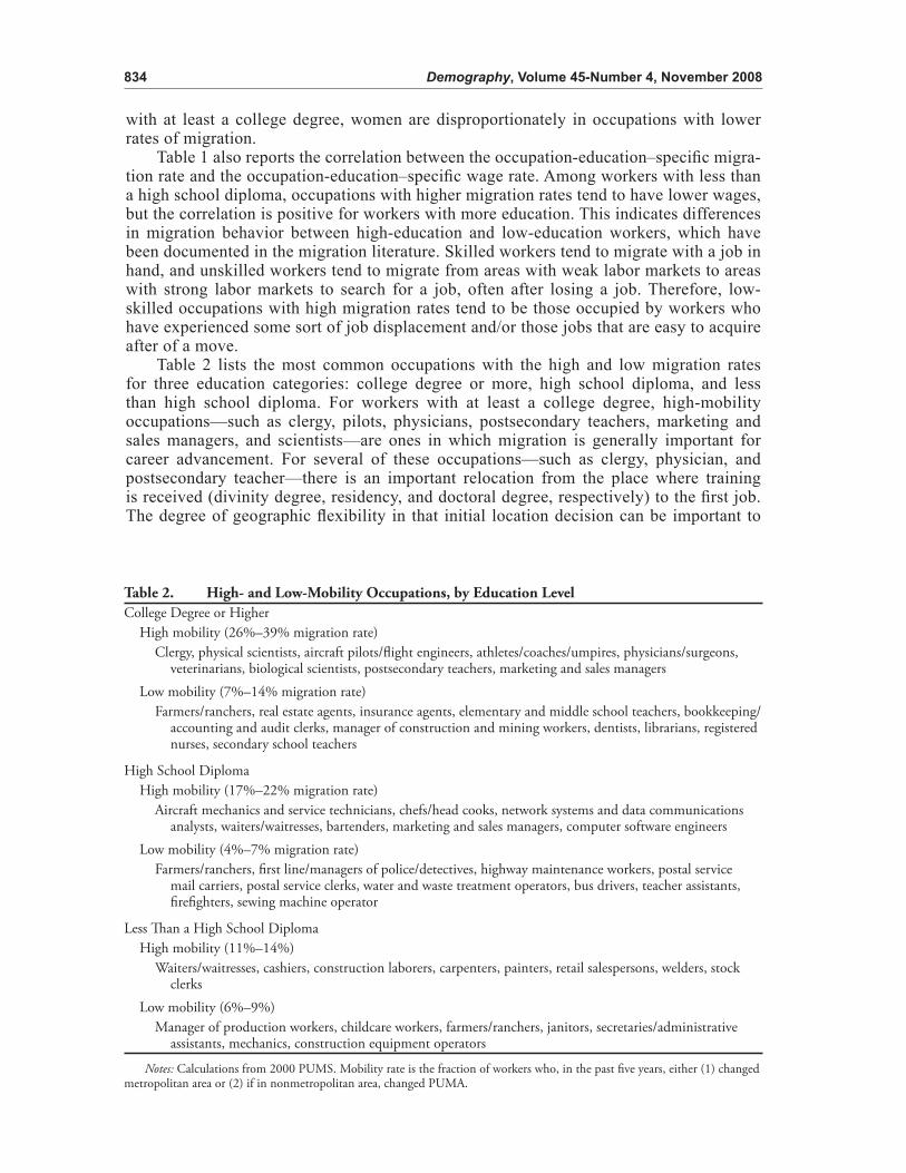
Table 2 lists the most common occupations with the high and low migration rates for three education categories: college degree or more, high school diploma, and less than high school diploma. For workers with at least a college degree, high-mobility occupations—such as clergy, pilots, physicians, postsecondary teachers, marketing and sales managers, and scientists—are ones in which migration is generally important for career advancement. For several of these occupations—such as clergy, physician, and postsecondary teacher—there is an important relocation from the place where training is received (divinity degree, residency, and doctoral degree, respectively) to the fi rst job. The degree of geographic fl exibility in that initial location decision can be important to

Table 2. High- and Low-Mobility Occupations, by Education LevelCollege Degree or Higher

High mobility (26%–39% migration rate)Clergy, physical scientists, aircraft pilots/fl ight engineers, athletes/coaches/umpires, physicians/surgeons,

veterinarians, biological scientists, postsecondary teachers, marketing and sales managersLow mobility (7%–14% migration rate)

Farmers/ranchers, real estate agents, insurance agents, elementary and middle school teachers, bookkeeping/accounting and audit clerks, manager of construction and mining workers, dentists, librarians, registered nurses, secondary school teachers

High School DiplomaHigh mobility (17%–22% migration rate)

Aircraft mechanics and service technicians, chefs/head cooks, network systems and data communications analysts, waiters/waitresses, bartenders, marketing and sales managers, computer software engineers

Low mobility (4%–7% migration rate)Farmers/ranchers, fi rst line/managers of police/detectives, highway maintenance workers, postal service

mail carriers, postal service clerks, water and waste treatment operators, bus drivers, teacher assistants, fi refi ghters, sewing machine operator

Less Th an a High School DiplomaHigh mobility (11%–14%)

Waiters/waitresses, cashiers, construction laborers, carpenters, painters, retail salespersons, welders, stock clerks

Low mobility (6%–9%)Manager of production workers, childcare workers, farmers/ranchers, janitors, secretaries/administrative

assistants, mechanics, construction equipment operators

Notes: Calculations from 2000 PUMS. Mobility rate is the fraction of workers who, in the past fi ve years, either (1) changed metropolitan area or (2) if in nonmetropolitan area, changed PUMA.


career advancement. In contrast, for those with a college degree or more in many of the low-mobility occupations—such as school teacher, insurance sales agent, and real estate agent—earnings increase by maintaining tenure in a single location, allowing a person to work his or her way up a pay scale or to establish a reputation and client base.

For members of the regression sample with a high school diploma, the high-mobility occupations are a mix of occupations in which relocation is a means of career advancement (e.g., aircraft mechanic and computer software engineer) and occupations in which it is not (e.g., cook, waitress/waiter, and bartender). For this latter set of jobs, it is highly unlikely the worker is migrating with a job in hand. Rather, these are jobs that a person, without a college degree, who has chosen to relocate (e.g., due to poor labor market opportunities in their previous location) can fi nd with relative ease.

Among workers with less than a high school diploma, the most common of the high-mobility occupations—waiter/waitress, cashier, retail salesperson, construction laborer, and stock clerk—are low-skilled and low-investment entry-level occupations with substantial employee turnover. These are, therefore, the most easily available jobs to migrating low-skilled workers, or to any entrant to a low-skilled labor market.

Regression SampleThe regression analysis in this article uses the sample from the 2000 census of married couples in which both the husband and wife are non-Hispanic, white, and native-born; are ages 25–55; and lived in the United States in 1995. The census asks individuals to report the occupation of the last job worked in the past fi ve years. Only couples with reported occupations for both members are included in the sample. Therefore, couples in which at least one member exhibits substantial detachment from the labor market (no employment in the past fi ve years) are excluded from the analysis. Couples that include a member of the military are excluded from the sample, as are couples in which marital status, education, occupation, earnings, or migration status are allocated for either partner.

In the regression analysis, couples are divided into four groups: both have a college degree (power couples), only husband has a college degree (husband-only couples), only wife has a college degree (wife-only couples), and neither has a college degree (neither-college couples). Couples are stratifi ed by educational attainment because the relationship between migration and earnings differs by education. Location choices are more likely important for career advancement for workers with college degrees. Of all married cou-ples with both members ages 25–55, 39.4% have at least one member with a college de-gree, and 18.6% are power couples. The percentages are higher in the regression sample (45.0% and 22.1%, respectively), largely because the sample is restricted to non-Hispanic white couples. Couples with nonwhite or Hispanic members are excluded from the analy-sis so that the samples are as homogenous as possible within educational grouping. Of married couples ages 25–55 in which at least one member has a college degree, 80.4% are non-Hispanic white.4

Table 3 reports sample means for each of these four categories of couples. A few striking patterns are notable. One is, of course, the difference in migration rates between high- and low-education couples that are also observed in Table 1. Another is that the college-educated men in power couples have higher-earning, higher-mobility occupations than the college-educated men in husband-only couples, and the college-educated women in power couples also have higher-earning, higher-mobility occupations than college-educated women in wife-only couples. This is consistent with positive assortative matching in which men with

4. Of interest would be to also estimate the models on samples of college-educated couples with nonwhite or Hispanic members. Space does not permit this analysis here. Additionally, the smaller sample sizes, the multiracial reporting in the census, and multiracial and multiethnic couples raise a host of additional empirical issues beyond what can be addressed in this article.


high earnings potential marry women with high earnings potential. As a result, the husbands in power couples have higher average earnings than those in husband-only couples, and the same is true for wives in power couples compared with those in wife-only couples.

It might be somewhat surprising that there are just as many wife-only couples as husband-only couples, but researchers have documented that it is now just as common for men to marry women with more education as it is for them to marry women with less education (Schwartz and Mare 2005). This is attributable, in part, to the fact that high school and college completion rates are now higher for women than for men. As might be expected, the wife-only couples are, on average, the youngest in the sample. Comparatively, the husband-only couples are, on average, the oldest in the sample.

The empirical specifi cations in this article treat spouse’s occupation as exogenous. This is, of course, a strong assumption, and it can be violated in a number of ways. One would be that particularly career-oriented individuals strategically chose partners in occu-pations with fewer career demands, thus generating negative assortative matching. Alter-natively, if there is positive assortative matching, career-oriented individuals will match

Table 3. Sample Means Power Husband Only Wife Only Neither Variables Couple College College College

Cross-Metropolitan Migration in the Past Five Years 0.193 0.158 0.130 0.104

Husband’s Earnings (if positive) 78,015 67,456 45,232 40,509 (71,592) (58,210) (37,567) (30,136)

Wife’s Earnings (if positive) 39,927 24,152 35,016 21,365 (40,185) (24,311) (27,340) (18,207)

Husband No Earnings 0.011 0.011 0.016 0.024Wife No Earnings 0.083 0.110 0.047 0.090Husband’s Occupation-Education 0.191 0.184 0.116 0.107

Migration Rate (0.058) (0.055) (0.034) (0.031)Wife’s Occupation-Education 0.173 0.115 0.164 0.107

Migration Rate (0.052) (0.031) (0.046) (0.031)Husband’s Occupation-Education 29.69 27.50 18.33 17.12

Average Wage (10.36) (9.27) (4.23) (3.75)Wife’s Occupation-Education 24.20 15.50 22.38 14.31

Average Wage (8.06) (4.04) (6.52) (3.56)Husband’s Education 13.62 13.35 10.37 9.58

(0.859) (0.671) (1.31) (1.63)Wife’s Education 13.47 10.60 13.31 9.80

(0.709) (1.20) (0.593) (1.48)Husband’s Age 41.30 43.32 40.44 41.35

(8.22) (7.70) (7.86) (7.76)Wife’s Age 39.75 41.26 38.78 39.51

(8.06) (7.70) (7.72) (7.69)Any Children Younger Th an 18 0.639 0.616 0.635 0.634Any Children Younger Th an 6 0.319 0.235 0.314 0.233N 168,990 88,375 86,901 420,846

Notes: Th e sample is as described in the notes of Table 1. Th e calculation of migration rate and average wage in occupation-education groups is also described in the notes of Table 1. Numbers in parentheses are standard deviations.


with individuals who are also in higher-paying, higher-mobility occupations.5 Finally, in-dividuals could change occupations during marriage in response to their partner’s success. For example, an artist with a low-earning spouse might take on alternative employment to supplement household income.

The earnings analysis in this article includes own-occupation fi xed-effects, so that the selective matching described in the preceding paragraph must take place within occupation and education class in order to be problematic. Even so, unobserved heterogeneity must be considered when interpreting the results in this article.

EMPIRICAL ANALYSISThe empirical analysis proceeds in two parts. The fi rst part estimates the effect of the migration rate in occupation-education class on an individual’s or a couple’s migration be-havior. A key component of this analysis is to compare the effect of occupational mobility on migration for married men and women with that for unmarried men and women. The second part of the analysis estimates the effect of the migration rate in spouse’s occupation-education class on labor market outcomes. The analysis focuses on the effect on the earn-ings of workers, but also considers the effects on employment.

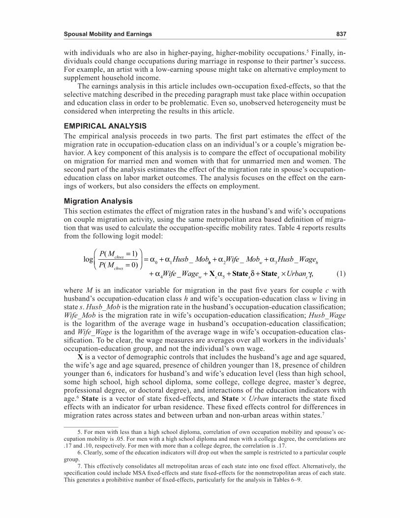
Migration AnalysisThis section estimates the effect of migration rates in the husband’s and wife’s occupations on couple migration activity, using the same metropolitan area based defi nition of migra-tion that was used to calculate the occupation-specifi c mobility rates. Table 4 reports results from the following logit model:

log( )( )

_P MP M

Husb Mobchws

chws

==

⎛

⎝⎜⎞

⎠⎟= +

10 0 1α α hh w hWife Mob Husb Wage+ +α α2 3_ _

+ + + + ×α α δ γ,4 5Wife Wage Urbanw c s s c_ X State State (1)

where M is an indicator variable for migration in the past fi ve years for couple c with husband’s occupation-education class h and wife’s occupation-education class w living in state s. Husb_Mob is the migration rate in the husband’s occupation-education classifi cation; Wife_Mob is the migration rate in wife’s occupation-education classifi cation; Husb_Wage is the logarithm of the average wage in husband’s occupation-education classifi cation; and Wife_Wage is the logarithm of the average wage in wife’s occupation-education clas-sifi cation. To be clear, the wage measures are averages over all workers in the individuals’ occupation-education group, and not the individual’s own wage.

X is a vector of demographic controls that includes the husband’s age and age squared, the wife’s age and age squared, presence of children younger than 18, presence of children younger than 6, indicators for husband’s and wife’s education level (less than high school, some high school, high school diploma, some college, college degree, master’s degree, professional degree, or doctoral degree), and interactions of the education indicators with age.6 State is a vector of state fi xed-effects, and State × Urban interacts the state fi xed effects with an indicator for urban residence. These fi xed effects control for differences in migration rates across states and between urban and non-urban areas within states.7

5. For men with less than a high school diploma, correlation of own occupation mobility and spouse’s oc-cupation mobility is .05. For men with a high school diploma and men with a college degree, the correlations are .17 and .10, respectively. For men with more than a college degree, the correlation is .17.

6. Clearly, some of the education indicators will drop out when the sample is restricted to a particular couple group.

7. This effectively consolidates all metropolitan areas of each state into one fi xed effect. Alternatively, the specifi cation could include MSA fi xed-effects and state fi xed-effects for the nonmetropolitan areas of each state. This generates a prohibitive number of fi xed-effects, particularly for the analysis in Tables 6–9.


The logit model in Eq. (1) is estimated on the sample described in Table 3, excluding two groups. Because the census does not record the year of marriage, one cannot confi rm that a migration in the fi ve years prior to the census was made as a couple. It is possible that the two individuals migrated independently, and then met and married. Following Cooke and Speirs (2005), couples that did not reside in the same PUMA in 1995 are, therefore, excluded from the analysis. This excludes 7.5% of the sample. Additionally, as discussed earlier, the census does not identify the MSA of residence for those couples residing in a PUMA that crosses an MSA boundary. Because I cannot correctly measure migration for residents of these cross-boundary PUMAs, I remove them from the analysis. This excludes an additional 10.5% of the sample.8

The fi rst two rows of Table 4 report average marginal effects for Husb_Mob and Wife_Mob, for each of the four groups of couples, using estimates from Eq. (1). Standard errors are obtained using multiway clustering on both husband’s and wife’s occupation-education groupings, using the method developed by Cameron, Gelbach, and Miller (2007). Standard errors for the marginal effects are calculated using the delta method. For all four groups of couples, both the husband’s and the wife’s occupation-specifi c mobility rates are positively related to the couple’s own migration propensity, but the effect of the husband’s mobility is considerably larger. In all four cases, the difference in the marginal effects of the husband’s and wife’s occupational mobility is statistically signifi cant at bet-ter than the 0.1% level.

These results indicate that the emphasis on the husband’s opportunities that has been observed in other studies of migration is not just the result of men and women having dif-ferent occupations with different mobility requirements. An occupation with a higher rate

8. Additional analysis was performed by using a state-based defi nition of migration, which avoids this loss of sample. The results were quite similar to those presented here.

Table 4. Eff ects of Mobility in Husband’s and Wife’s Occupations on Migration in the Past Five Years

Power Husband Only Wife Only NeitherVariables Couple College College College

Husband’s Occupation-Education Migration Rate 0.678*** 0.693*** 0.709*** 0.655*** (0.041) (0.040) (0.051) (0.030)

Wife’s Occupation-Education Migration Rate 0.376*** 0.462*** 0.368*** 0.427*** (0.040) (0.054) (0.045) (0.034)

Husband’s Occupation-Education Average Wage 0.018* 0.028*** 0.011 0.022*** (0.009) (0.008) (0.007) (0.004)

Wife’s Occupation-Education Average Wage –0.028*** –0.050*** 0.013* –0.010*** (0.006) (0.005) (0.005) (0.003)

N 138,738 73,005 69,050 343,628

Notes: Th e sample is the same as described in Table 1 with the exclusion of couples who (1) did not live in the same PUMA in 1995 or (2) lived in an unidentifi ed MSA area in 1995 or 2000. Th e table reports average marginal eff ects from the logit model described in Eq. (1), in which the dependent variable is an indicator for migration in the past fi ve years. Th e measure-ment of migration, explanatory variables, and couple groupings are described in notes of Tables 1 and 3. Th e model includes controls for the husband’s age and age squared, the wife’s age and age squared, presence of children younger than 18, presence of children younger than 6, indicators for the husband’s and the wife’s education level (less than high school, some high school, high school diploma, some college, college degree, master’s degree, professional degree, or doctoral degree), interactions of the education indicators with age, and state fi xed-eff ects and state-urban fi xed-eff ects. Standard errors for average marginal eff ects (shown in parentheses) are calculated using the delta method and with multiway clustering on both the husband’s and the wife’s occupation-education groupings, using method of Cameron, Gelbach, and Miller (2007).

*p < .05; **p < .01; ***p < .001


of migration for either member of the household will increase the probability the couple migrates, but more so when it is the husband’s occupation than when it is the wife’s. Inter-estingly, the average marginal effects are relatively similar in size across all four groups of couples. To illustrate the magnitude of the effect, an increase by 1 standard deviation (0.058) in husband’s occupational mobility for a power couple increases the probability of migration of the power couple, on average, by 3.9 percentage points. The baseline migra-tion rate for power couples is 19.3%.

The fi nal two rows of Table 4 report average marginal effects of Husb_Wage and Wife_Wage. For all but the wife-only couples, a higher wage in the husband’s occupation increases the probability of migration, and a higher wage in the wife’s occupation lowers it. For the couples in which only the wife has a college degree, the effects are reversed. The wife’s occupational wage has a positive effect on migration, and husband’s occupational wage has no effect.

Migration Analysis: Never-Married Versus MarriedThe results in Table 4 show that husband’s and wife’s occupational mobility rates do not have equal effects on the couple’s migration decisions. This could indicate that the hus-band’s and the wife’s careers do not receive equal weight in household decisions. But, these results could also indicate that men and women have different preferences with respect to migration and careers. It could be that women are generally less responsive to migration op-portunities in their occupation. To further address this issue, Table 5 provides estimates of the effect of occupational mobility on migration behavior for never-married individuals.

The fi rst row of Table 5 reports results for never-married, white, non-Hispanic, native-born individuals, ages 25–55, who meet the same sample selection requirements as the married couples sample. The table reports results from the following logit model:

log( )( )

_P MP M

Own Mobios

ioso o

==

⎛

⎝⎜⎞

⎠⎟= + +

10 1α α α22Own Wageo_

+ + + ×X State Statei s s iUrbanα δ γ,3 (2)

where M remains an indicator for migration in the previous fi ve years for person i in occu-pation o in state s, Own_Mob is the migration rate in the individual’s occupation-education classifi cation, and Own_Wage is the average wage in the individual’s occupation-education classifi cation. X contains the same individual controls for education, age, and presence of children as described earlier for Eq. (1), excluding, of course, the controls for spouse’s demographic characteristics.9

Average marginal effects of Own_Mob are reported in the fi rst row of Table 5 for never-married men and women with and without a college degree. The results indicate that among those with at least a college degree, never-married men and never-married women are equally—and highly—responsive to occupational mobility in their migration behavior.10 Among never-married individuals with less than a college degree, the migration behavior of women is less responsive to occupational mobility than the migration behavior of men.

The second and third rows of Table 5 report estimates from Eq. (2) for the sample of married individuals. The specifi cation in the second row is identical to the one used for unmarried individuals in the fi rst row, and the third row adds controls for spouse’s

9. Because the “own children in household” variable is reported only for women, the controls for presence of children are omitted in the models for unmarried men. This is unlikely to generate much bias in the results for unmarried men. Further, the results in Table 5 change only modestly when the controls for children are omitted from all models.

10. This fi nding is similar to that of Jurges (2006), who found no gender differences in the determinants of migration among single men and women in Germany.


characteristics.11 For all groups, the marginal effects of occupational mobility are lower for married individuals than for never-married individuals. It is noteworthy, however, that the change is the most precipitous for college-educated women. The fi nal row of Table 5 generates the same fi ndings as those reported in Table 4: a substantially larger effect of the husband’s mobility on a married couple’s migration than the wife’s mobility, and very similar effects across education categories. The results in Table 5, however, indicate that this asymmetry is unique to marriage and is not due to underlying differences in the migration behavior of college-educated men and women. Such asymmetry could result from an effect of marriage on college-educated women, or selection into marriage by less career-oriented women. In contrast, the results for low-education women indicate a lower baseline mobility among never-married women compared with men.

Earnings AnalysisThis section analyzes the relationship between an individual’s own earnings and the occupation-specifi c migration rate of the spouse. The sample is that described in Table 3, but only including those couples in which both members have positive earnings in 1999. Table 4 reports the results from the following regression specifi cation (Eq. (3)):

Earn Own Mob Spouse Mob Owniops o o p= + + +β β β β1 2 3_ _ _WWage Spouse Wageo p+ β4 _

+ β + φ + ρ + ψ + εX Occ State Statei o s s i iopsUrban5 × , (3)

where Earn is the logarithm of total earnings in 1999 for person i in occupation-education classifi cation o with spouse’s occupation-education classifi cation p living in state s. Total earnings are the sum of reported wage and salary earnings and self-employment earnings

11. The specifi cation used to produce the results in the third row of Table 5 is identical to that used in Table 4, except that the estimates are pooled across spouse’s education; and in Table 4, they are estimated separately based on the spouse’s education.

Table 5. Eff ects of Occupational Mobility on Migration in the Past Five Years, Comparison of Single and Married Individuals

College-Educated Less Th an College-Educated ________________________ _________________________Marital Status Men Women Men Women

Never-Married 0.902 0.943 1.01 0.735 (0.052) (0.073) (0.048) (0.046)

N 82,920 81,524 147,487 90,796Married

No spousal controls 0.717 0.528 0.695 0.486 (0.036) (0.043) (0.031) (0.037)With spousal controls 0.685 0.366 0.664 0.430 (0.038) (0.038) (0.029) (0.032)N 211,745 207,796 412,678 416,636

Notes: Th e table reports average marginal eff ects of mobility in occupation-education class from the logit model described in Eq. (2), which includes controls for average wage in occupation-education class, age and age squared, presence of children younger than 18, presence of children younger than 6, education level (less than high school, some high school, high school diploma, some college, college degree, master’s degree, professional degree, or doctoral degree), interactions of the education indicators with age, state fi xed-eff ects, and state-urban fi xed-eff ects. In the last row, controls for spouse’s occupational and demographic characteristics are also included. Standard errors are shown in parentheses.


in 1999. Own_Mob is the migration rate in the individual’s occupation-education classifi -cation, and Spouse_Mob is the migration rate in his or her spouse’s occupation-education classifi cation. Similarly, Own_Wage and Spouse_Wage are the average wages in the own and spouse occupation-education classifi cations. X contains the same controls for age, education, and children as defi ned earlier for Eq. (1). Occupation is a vector of occupa-tion fi xed-effects for the 504 occupation categories. State and State × Urban are state and state-urban fi xed-effects as defi ned earlier for Eq. (1).

Including occupation fi xed-effects and the average wage within the individual’s occupation-education classifi cation controls for an enormous amount of heterogeneity in the individual’s earnings potential. I am primarily interested in β2 (the effect of the spouse’s mobility) rather than β1 (the effect of own mobility). With the occupation fi xed effects, β1 is identifi ed only by the variation in mobility across different education groups within occupation, which makes it diffi cult to interpret. The coeffi cient on spouse’s mobility, β2, indicates whether higher occupational mobility for the spouse is associated with earnings that are above average or below average for an individual’s occupation.

The estimates of β2 from Eq. (3) are reported for the full sample of married couples in the fi rst column of Table 6. Standard errors are clustered by spouse’s occupation-education group. The fi rst coeffi cient of 0.029 indicates that among power couples, the wife’s mobility has a small and insignifi cant effect on husband’s earnings. The second coeffi cient, –1.01, indicates that among power couples, the husband’s mobility has a sizeable and statistically signifi cant negative effect on wife’s earnings. The magnitude is such that if the husband’s occupational mobility is 1 standard deviation (0.058) higher, this reduces the wife’s earnings by 5.9%. The results for couples in which only the husband has a college degree are nearly identical to those for power couples. For both power couples and husband-only couples, the difference in the β2 coeffi cients in the husband’s and the wife’s equations is signifi cant at better than the 0.1% level. These fi ndings are consistent with the case in which having a husband in a high-migration occupation increases the likelihood that the wife will be dis-advantaged by the household’s location. The fi ndings likewise suggest that a more-mobile wife does not generally generate disadvantageous location decisions for the husband.

Because the variation in spouse’s occupation (even within occupation and couple group) is not strictly exogenous, alternative interpretations are also possible. The large negative effect of a husband’s mobility on his wife’s earnings could refl ect the fact that men in highly mobile careers seek out wives with less career ambition and lower earnings. However, if this selective matching occurs largely based on occupation, so that career- oriented and mobile men seek out wives who are (for example) elementary school teachers, the occupation fi xed-effects will control for this effect. The analysis in Table 6 measures the effect of husband’s mobility on wives within the same occupation and education group, comparing (for example) female elementary school teachers married to high-mobility hus-bands with elementary school teachers married to low-mobility husbands. Additionally, the matching on observables suggest positive, rather than negative, assortative matching. For power couples, there is a positive correlation between the husband’s and the wife’s occu-pational mobility (.17), between the husband’s and the wife’s occupational wage (.22), and between the husband’s earnings and the wife’s earnings (.14). This suggests that at least based on observable variables, men who are more career-oriented tend to marry women who are more career-oriented.

The results differ dramatically when considering couples in which only the wife has a college degree. The negative effect of the husband’s mobility on the wife’s earnings is much smaller and insignifi cant compared with couples in which the husband has a college degree. Among the wife-only couples, there is no signifi cant difference in the coeffi cients in the husband’s and the wife’s equations. It does not appear that these women are disadvantaged in their location choice by their husband’s occupational mobility. This could indicate that these marriages are more egalitarian. It could also be that the earnings differ less by location


for the low-education husbands in these marriages, thus reducing the probability that the wife will be a tied mover or a tied stayer.

The results for couples in which neither member has a college degree are quite dif-ferent from the rest of the sample. The coeffi cient on the wife’s mobility in the husband’s regression is negative and signifi cant, but there is no effect of the husband’s mobility on the wife’s earnings. Although one interpretation would be that in low-education couples, men experience disadvantageous location choices, a look at the high-mobility occupations for low-education women (listed in Table 2) suggests an alternative interpretation. Given that the high-mobility jobs for low-education women tend to be jobs as waitresses, retail salespersons, and cashiers, a reasonable interpretation is that the below-average earnings of the husband cause low-skilled wives to take jobs in these low-skilled occupations, either with or without a relocation, to supplement household income.

Table 6. Eff ect of Spouse’s Occupational Mobility on Own Earnings β2 Estimate __________________________________________________ Full No Child Child YoungerCouple Type Sample Younger Th an 18 Th an 18

Power CoupleHusband 0.029 –0.031 0.078 (0.076) (0.082) (0.088)Wife –1.01*** –0.594*** –1.26*** (0.176) (0.110) (0.219)N 153,362 58,293 95,069

Husband Only CollegeHusband –0.044 0.246 –0.209 (0.201) (0.178) (0.250)Wife –1.01*** –0.748*** –1.15*** (0.220) (0.146) (0.284)N 77,874 31,096 46,778

Wife Only CollegeHusband –0.042 –0.058 –0.012 (0.077) (0.127) (0.076)Wife –0.152 –0.079 –0.246 (0.210) (0.154) (0.272)N 80,901 30,088 50,813

Neither CollegeHusband –0.669*** –0.583*** –0.701*** (0.152) (0.157) (0.153)Wife –0.117 0.045 –0.225 (0.175) (0.176) (0.192) N 374,284 139,700 234,584

Notes: Th e sample is as described in Table 1, excluding couples in which either partner is without earnings in 1999. Dependent variable is the logarithm of own earnings in 1999. Th e table reports es-timates of β2 from Eq. (3), which is the coeffi cient on the migration rate in the spouse’s occupation-education group. Measurement of explanatory variables and couple groupings are described in the notes of Tables 1 and 3. Regressions include the same controls listed in the notes of Table 4, with the addition of occupation fi xed-eff ects. Standard errors, shown in parentheses, are clustered by spouse’s occupation-education group.

***p < .001


The remaining two columns of Table 6 estimate Eq. (3) separately for couples with and without children under the age of 18. For all four of the couple groups, the negative effects of the husband’s mobility on the wife’s earnings are more pronounced in couples with children under the age of 18. The differences in effects for mothers and nonmothers are statistically signifi cant at the 5% level for all but the wife-only couples. These results are similar to those of Cooke (2001), who found that the negative effects of migration on employment are stronger and of longer duration for mothers than nonmothers. These re-sults could indicate that couples with young children are particularly likely to place more weight on the husband’s career in making location choices. Alternatively, the weights may not change, but it may be that nonoptimal location choices are even more costly to mothers because, for example, they disrupt childcare arrangements.

The remaining analysis in the article considers three extensions of the earnings re-sults displayed in Table 6. The fi rst extension is to further differentiate power couples based on whether one or both spouses have an advanced degree. These results are re-ported in Table 7. The second extension considers that the analysis in Table 6 is limited to dual-earning couples, which ignores the fact that some individuals might not be employed because of the couple’s location choices. Analysis of non-earners is, therefore, presented in Table 8. Finally, the earnings analysis in Tables 6–8 does not make any use of informa-tion regarding whether a couple has actually migrated—only what the migration rate is in the husband’s and the wife’s occupation. Table 9 reports earnings results separately by migration status.

Super Power CouplesAn interesting extension of the analysis in Table 6 is to further differentiate power couples based on whether one or both of the spouses have an advanced degree. Presumably, this might further refi ne the sample to workers who are more likely to be career- oriented and for whom location is a factor in career advancement and earnings. Using only the sample of dual-earner power couples from Table 6, Table 7 reports earnings results for “super power” couples (both have an advanced degree), couples in which only the husband has an advanced degree, and couples in which only the wife has an advanced degree. Couples in which either member has less than a college degree are excluded from Table 7. The results in Table 7 strongly resemble those in Table 6. For couples in which the husband has an advanced degree (regardless of whether the wife does), the wife experiences large, signifi -cant negative effects of husband’s mobility. This negative effect is substantially reduced for couples in which only the wife has an advanced degree. For all three types of couples, the β2 coeffi cients in the husband’s and wife’s equations are statistically different at better than the 5% level. For all three types of couples, the negative effects are also larger for women with young children, although the difference is again not statistically signifi cant for wife-only couples.

Interestingly, 33% of wives in super power couples are employed in primary or sec-ondary education, as are 37% of wives in wife-only advanced degree couples. This is a result of the high proportion of college-educated women who work in primary or secondary education, and the strong incentives for public school teachers to obtain a master’s degree in education to move up on the school district pay schedule. As a sensitivity test, I reas-signed all observations in Table 7 with an advanced degree and employment in primary or secondary education to an education level of college degree. This had a very modest effect on the results.12

12. Reassigning teachers with advanced degrees changes the coeffi cient in the women’s regressions from –1.16 to –0.98 for super power couples, from –1.36 to –1.38 for husband-only couples, and from –0.408 to –0.355 for wife-only couples.


Analysis of Non-EarnersThe analyses in Tables 6 and 7 are conducted only on the sample of couples in which both members have positive earnings in 1999. One concern could be that by focusing only on earners, this analysis understates the full effect on labor market outcomes. A disadvanta-geous labor market location could cause individuals to become unemployed or drop out of the labor market entirely. The analysis in Table 8 includes both earners and non-earners, as long as they have worked a job in the past fi ve years. I do not have information on oc-cupation for those who have not worked in the past fi ve years. The model used in Table 8 estimates whether having a spouse in a high-mobility occupation makes one more likely to be a non-earner (and therefore to be omitted from the analyses in Tables 6 and 7).

The dependent variable is an indicator that equals 1 if earnings in 1999 are less than or equal to zero.13 The very large number of occupational fi xed-effects in this model becomes prohibitive in the estimation of a logit model, so a linear probability model is used instead:

13. The vast majority of the non-earners have zero earnings, but about 20% of the men and 4% of the women report negative earnings from self-employment. Removing these individuals from the analysis has a very minor effect on the results.

Table 7. Eff ect of Spouse’s Occupational Mobility on Own Earnings, Super Power Couples

β2 Estimate __________________________________________________ Full No Child Child YoungerCouple Type Full Sample Younger Th an 18 Th an 18

Super Power CoupleHusband –0.157 –0.197 –0.114 (0.097) (0.129) (0.111)Wife –1.16*** –0.753*** –1.40*** (0.167) (0.148) (0.193)N 32,368 12,303 20,065

Husband Only Advanced DegreeHusband 0.206 0.169 0.266 (0.149) (0.232) (0.183)Wife –1.36*** –0.597*** –1.78*** (0.207) (0.157) (0.237)N 30,791 11,294 19,497

Wife Only Advanced DegreeHusband 0.036 0.089 0.030 (0.105) (0.105) (0.142)Wife –0.408* –0.212 –0.581** (0.174) (0.166) (0.216)N 25,151 10,275 14,876

Notes: Th e sample is restricted to the dual-earner power couples used in the fi rst row of Table 6. Super power couples are those in which both members have an advanced degree (master’s, professional, or doctor-ate). Th e model is the same earnings regression estimated in Table 6. Standard errors, shown in parentheses, are clustered by spouse’s occupation-education group.

*p < .05; **p < .01; ***p < .001


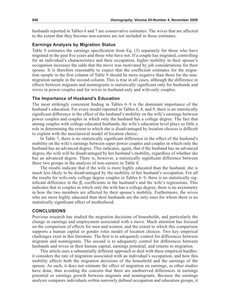
I Earnings Own Mob Spouse Moiops o o( ) _ _≤ = + +0 1 2β β β bb Own Wagep o+ β3 _

+ + + +β β ρ4 5Spouse Wagep i o s_ X Occ Stateφ

+ × +States i iopsUrban ψ ε . (4)

The right side of Eq. (4) is the same as that used in Eq. (3) earlier.Eq. (4) is estimated for all the education groups used in Tables 6 and 7. The results, re-

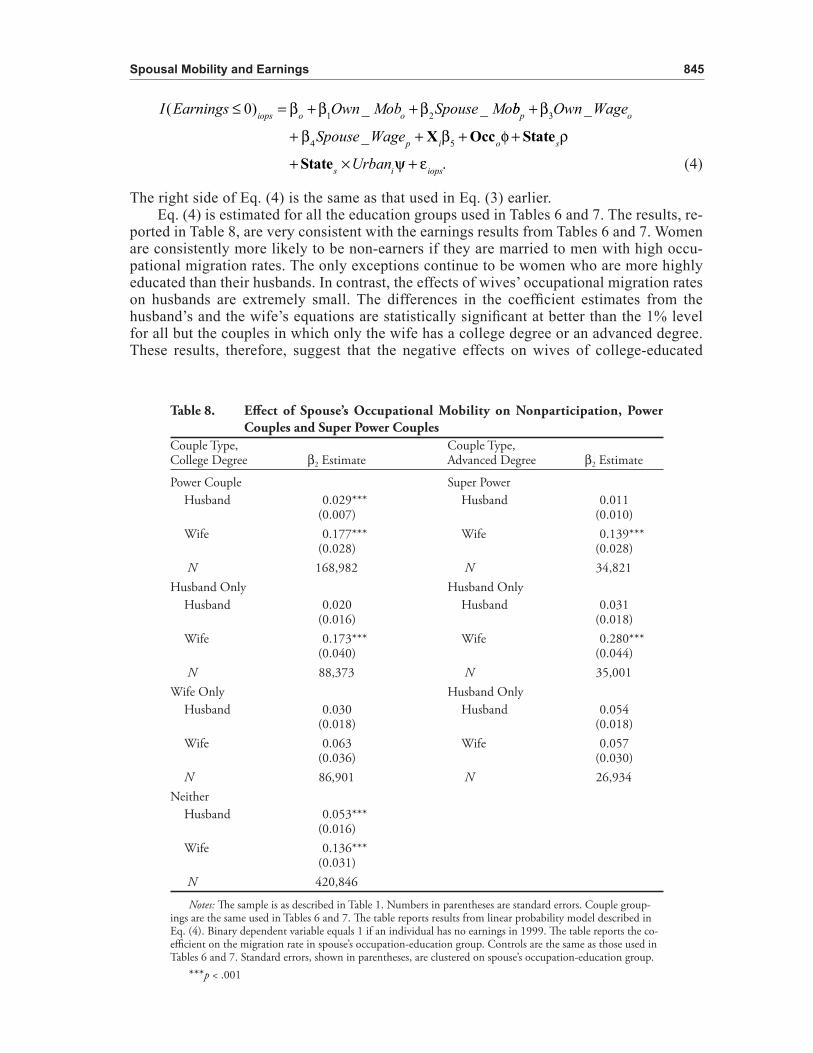
ported in Table 8, are very consistent with the earnings results from Tables 6 and 7. Women are consistently more likely to be non-earners if they are married to men with high occu-pational migration rates. The only exceptions continue to be women who are more highly educated than their husbands. In contrast, the effects of wives’ occupational migration rates on husbands are extremely small. The differences in the coeffi cient estimates from the husband’s and the wife’s equations are statistically signifi cant at better than the 1% level for all but the couples in which only the wife has a college degree or an advanced degree. These results, therefore, suggest that the negative effects on wives of college-educated

Table 8. Eff ect of Spouse’s Occupational Mobility on Nonparticipation, Power Couples and Super Power Couples

Couple Type, Couple Type,College Degree β2 Estimate Advanced Degree β2 Estimate

Power Couple Super PowerHusband 0.029*** Husband 0.011 (0.007) (0.010)Wife 0.177*** Wife 0.139*** (0.028) (0.028) N 168,982 N 34,821

Husband Only Husband OnlyHusband 0.020 Husband 0.031 (0.016) (0.018)Wife 0.173*** Wife 0.280*** (0.040) (0.044) N 88,373 N 35,001

Wife Only Husband OnlyHusband 0.030 Husband 0.054 (0.018) (0.018)Wife 0.063 Wife 0.057 (0.036) (0.030)N 86,901 N 26,934

NeitherHusband 0.053*** (0.016) Wife 0.136*** (0.031) N 420,846

Notes: Th e sample is as described in Table 1. Numbers in parentheses are standard errors. Couple group-ings are the same used in Tables 6 and 7. Th e table reports results from linear probability model described in Eq. (4). Binary dependent variable equals 1 if an individual has no earnings in 1999. Th e table reports the co-effi cient on the migration rate in spouse’s occupation- education group. Controls are the same as those used in Tables 6 and 7. Standard errors, shown in parentheses, are clustered on spouse’s occupation-education group.

***p < .001


husbands reported in Tables 6 and 7 are conservative estimates. The wives that are affected to the extent that they become non-earners are not included in those estimates.

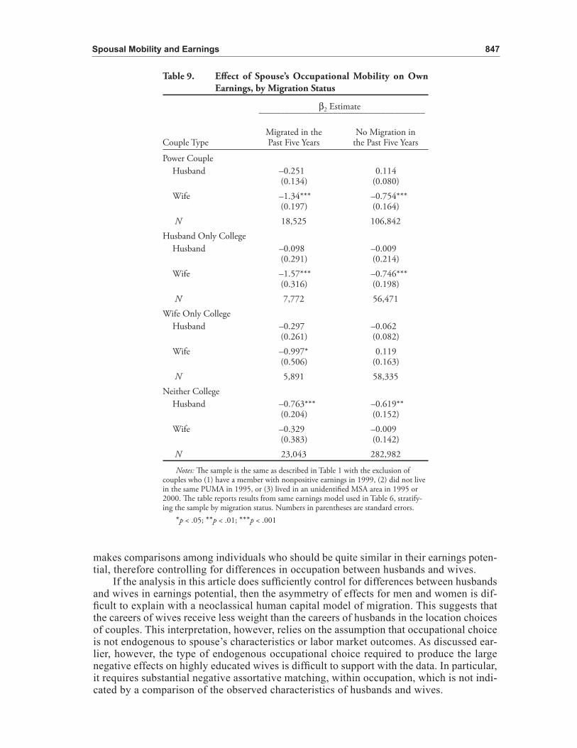
Earnings Analysis by Migration StatusTable 9 estimates the earnings specifi cation from Eq. (3) separately for those who have migrated in the past fi ve years and those who have not. If a couple has migrated, controlling for an individual’s characteristics and their occupation, higher mobility in their spouse’s occupation increases the odds that the move was motivated by job considerations for their spouse. It is therefore reasonable to expect that the coeffi cient estimates for the migra-tion sample in the fi rst column of Table 9 should be more negative than those for the non-migration sample in the second column. This is true in all cases, although the difference in effects between migrants and nonmigrants is statistically signifi cant only for husbands and wives in power couples and for wives in husband-only and wife-only couples.

The Importance of Husband’s EducationThe most strikingly consistent fi nding in Tables 6–9 is the dominant importance of the husband’s education. For every model reported in Tables 6, 8, and 9, there is no statistically signifi cant difference in the effect of the husband’s mobility on the wife’s earnings between power couples and couples in which only the husband has a college degree. The fact that among couples with college-educated husbands, the wife’s education level plays so little a role in determining the extent to which she is disadvantaged by location choices is diffi cult to explain with the neoclassical model of location choice.

In Table 7, there is no statistically signifi cant difference in the effect of the husband’s mobility on the wife’s earnings between super power couples and couples in which only the husband has an advanced degree. This indicates, again, that if the husband has an advanced degree, the wife will be disadvantaged by her husband’s mobility, regardless of whether she has an advanced degree. There is, however, a statistically signifi cant difference between these two groups in the analysis of non-earners in Table 8.

The results indicate that if the wife is more highly educated than the husband, she is much less likely to be disadvantaged by the mobility of her husband’s occupation. For all the results for wife-only college degree couples in Tables 6–9, there is no statistically sig-nifi cant difference in the β2 coeffi cients in the husband’s and the wife’s regressions. This indicates that in couples in which only the wife has a college degree, there is no asymmetry in how the two members are affected by their spouse’s mobility. Furthermore, the wives who are more highly educated than their husbands are the only ones for whom there is no statistically signifi cant effect of motherhood.

CONCLUSIONSPrevious research has studied the migration decisions of households, and particularly the change in earnings and employment associated with a move. Much attention has focused on the comparison of effects for men and women, and the extent to which this comparison supports a human capital or gender roles model of location choices. Two key empirical challenges exist in this literature. The fi rst is to adequately control for differences between migrants and nonmigrants. The second is to adequately control for differences between husbands and wives in their human capital, earnings potential, and returns to migration.

This article uses a substantially different approach to deal with these empirical hurdles: it considers the rate of migration associated with an individual’s occupation, and how this mobility affects both the migration decisions of the household and the earnings of the spouse. As such, it does not estimate the effect of migration on earnings, as other studies have done, thus avoiding the concern that there are unobserved differences in earnings potential or earnings growth between migrants and nonmigrants. Because the earnings analysis compares individuals within narrowly defi ned occupation and education groups, it


makes comparisons among individuals who should be quite similar in their earnings poten-tial, therefore controlling for differences in occupation between husbands and wives.

If the analysis in this article does suffi ciently control for differences between husbands and wives in earnings potential, then the asymmetry of effects for men and women is dif-fi cult to explain with a neoclassical human capital model of migration. This suggests that the careers of wives receive less weight than the careers of husbands in the location choices of couples. This interpretation, however, relies on the assumption that occupational choice is not endogenous to spouse’s characteristics or labor market outcomes. As discussed ear-lier, however, the type of endogenous occupational choice required to produce the large negative effects on highly educated wives is diffi cult to support with the data. In particular, it requires substantial negative assortative matching, within occupation, which is not indi-cated by a comparison of the observed characteristics of husbands and wives.

Table 9. Eff ect of Spouse’s Occupational Mobility on Own Earnings, by Migration Status

β2 Estimate ______________________________________

Migrated in the No Migration inCouple Type Past Five Years the Past Five Years

Power CoupleHusband –0.251 0.114 (0.134) (0.080)Wife –1.34*** –0.754*** (0.197) (0.164) N 18,525 106,842

Husband Only CollegeHusband –0.098 –0.009 (0.291) (0.214)Wife –1.57*** –0.746*** (0.316) (0.198) N 7,772 56,471

Wife Only CollegeHusband –0.297 –0.062 (0.261) (0.082)Wife –0.997* 0.119 (0.506) (0.163) N 5,891 58,335

Neither CollegeHusband –0.763*** –0.619** (0.204) (0.152)Wife –0.329 –0.009 (0.383) (0.142) N 23,043 282,982

Notes: Th e sample is the same as described in Table 1 with the exclusion of couples who (1) have a member with nonpositive earnings in 1999, (2) did not live in the same PUMA in 1995, or (3) lived in an unidentifi ed MSA area in 1995 or 2000. Th e table reports results from same earnings model used in Table 6, stratify-ing the sample by migration status. Numbers in parentheses are standard errors.

*p < .05; **p < .01; ***p < .001


The most striking fi nding is that the earnings disadvantage experienced by wives is determined largely by their husbands’ education, rather than by their own educational attainment. This again suggests that the career prospects of husbands and wives do not receive equal weight in household decisions. There are a number of reasons why the labor market outcomes of women still lag behind those of men, despite their higher rates of col-lege completion. This article suggests that one contributing factor is that married women with college degrees are often unable to make optimal location decisions and that their earnings suffer as a result.

REFERENCESAstrom, J. and O. Westerlund. 2006. “Sex and Migration: Who is the Tied Mover?” Unpublished

manuscript. Department of Economics, Umeå University, Umeå, Sweden.Bailey, A.J. and T.J. Cooke. 1998. “Family Migration and Employment: The Importance of Migration

History and Gender.” International Regional Science Review 21:99–118.Basker, E. 2003. “Education, Job Search and Migration.” Working Paper 02-17. Department of Eco-

nomics, University of Missouri–Columbia.Bielby, W.T. and D.D. Bielby. 1992. “I Will Follow Him: Family Ties, Gender-Role Beliefs, and

Reluctance to Relocate for a Better Job.” American Journal of Sociology 97:1241–67.Boyle, P., T. Cooke, K. Halfacree, and D. Smith. 1999. “Gender Inequality in Employment Status

Following Family Migration in GB and the US: The Effect of Relative Occupational Status.” International Journal of Sociology and Social Policy 19(9):109–43.

———. 2001. “A Cross-National Comparison of the Impact of Family Migration on Women’s Em-ployment Status.” Demography 38:201–13.

———. 2002. “A Cross-National Study of the Effects of Family Migration on Women’s Labor Market Status.” Journal of the Royal Statistical Society Series A 165:465–80.

Cameron, C.A., J.B Gelbach, and D.L. Miller. 2007. “Robust Inference With Multi-way Clustering.” Technical Working Paper No. 327. National Bureau of Economic Research, Cambridge, MA.

Clark, W.A.V. and Y.Q. Huang. 2006. “Balancing Move and Work: Women’s Labour Market Exits and Entries After Family Migration.” Population, Space and Place 12:31–44.

Clark, W.A.V. and S.D. Withers. 2002. “Disentangling the Interaction of Migration, Mobility and Labor-Force Participation.” Environment and Planning A 34:923–45.

Compton, J. and R.A. Pollak. 2007. “Why Are Power Couples Increasingly Concentrated in Large Metropolitan Areas?” Journal of Labor Economics 25:475–512.

Cooke, T.J. 2001. “‘Trailing Wife’ or ‘Trailing Mother’? The Effects of Parental Status on the Re-lationship Between Family Migration and the Labor-Market Participation of Married Women.” Environment and Planning A 33:419–30.

———. 2003. “Family Migration and the Relative Earnings of Husbands and Wives.” Annals of the Association of American Geographers 93:338–49.

Cooke, T.J. and A.J. Bailey. 1996. “Family Migration and the Employment of Married Women and Men.” Economic Geography 72:38–48.

Cooke, T.J. and K. Speirs. 2005. “Migration and Employment Among the Civilian Spouses of Mili-tary Personnel.” Social Science Quarterly 86:343–55.

Costa, D.L. and M.E. Kahn. 2000. “Power Couples: Changes in the Location Choice of the College Educated, 1940–1990.” Quarterly Journal of Economics 53:648–64.

Duncan, R.P. and C.C. Perrucci. 1976. “Dual Occupation Families and Migration.” American Socio-logical Review 41:252–61.

Jacobsen, J.P. and L.M. Levin. 1997. “Marriage and Migration: Comparing Gains and Losses From Migration for Couples and Singles.” Social Science Quarterly 78:688–709.

———. 2000. “The Effects of Internal Migration on the Relative Economic Status of Women and Men.” Journal of Socio-Economics 29:291–304.

Jurges, H. 2006. “Gender Ideology, Division of Housework, and the Geographic Mobility of Fami-lies.” Review of Economics of the Household 4:299–324.


LeClere, F.B. and D.K. McLaughlin. 1997. “Family Migration and Changes in Women’s Earnings: A Decomposition Analysis.” Population Research and Policy Review 16:315–35.

Mincer, J.F. 1978. “Family Migration Decisions.” Journal of Political Economy 86:749–74.Morrison, D. and D. Lichter. 1988. “Family Migration and Female Employment.” Journal of Mar-

riage and the Family 50:161–72.Nivalainen, S. 2004. “Determinants of Family Migration: Short Moves vs. Long Moves.” Journal of

Population Economics 17:157–75.Rabe, B. 2006, “Dual-Earner Migration in Britain. Earnings Gains, Employment, and Self-selection.”

Working paper. Institute for Social and Economic Research, Ruhr-University Bochum.Sandell, S.H. 1977. “Women and the Economics of Family Migration.” Review of Economics and

Statistics 59:406–14.Schwartz, C.R. and R.D. Mare. 2005. “Trends in Educational Assortative Marriage.” Demography

42:621–46.Shauman, K.A. and M.C. Noonan. 2007. “Family Migration and Labor Force Outcomes: Sex Differ-

ences in Occupational Context.” Social Forces 85:1735–64.Shihadeh, E.S. 1991. “The Prevalence of Husband-Centered Migration: Employment Consequences

for Married Mothers.” Journal of Marriage and the Family 53:432–44.Spitze, G. 1984. “The Effects of Family Migration on Wives’ Employment: How Long Does It Last?”

Social Science Quarterly 65:21–36.

Documents

SPOUSAL MOBILITY AND EARNINGS* - …spot.colorado.edu/~mckinnis/McKinnishDemography.pdf · migration (Clark and Huang 2006; Cooke 2001, 2003; Jacobsen and Levin 1997). There are still,