Embed Size (px)
Citation preview
Spousal Mobility and Earnings*
by Terra McKinnish Economics Dept
University of Colorado Boulder, CO 80309-0256 [email protected]
303-492-6770
April 2008
*Helpful comments from Robert Pollak and Ernesto Villanueva, as well as participants at the 2006 ESPE meetings, the 2007 ASSA meetings and the 2007 SOLE meetings and seminar participations at the University of Colorado-Boulder and University of Colorado-Denver are gratefully acknowledged.
Abstract
In the substantial literature on the relationship between migration and earnings, an important finding has been that the earnings of married women typically decrease with a move while the earnings of married men often increase. This is consistent with the story that married women are more likely to act as the “trailing spouse” or to be a “tied-mover.” This paper considers a related but largely unexplored question: what is the effect of having an occupation that is associated with frequent migration on the migration decisions of your household and on the earnings of your spouse? How do these effects differ between men and women?
The Public Use Microdata Sample from the 2000 Decennial Census is used to calculate 5-year metropolitan-based migration rates by occupation and education. The analysis estimates the effects of these occupational mobility measures on the migration of couples and the earnings of married individuals. Analysis is conducted separately for four groups of couples: both have college degrees (“power couples”), only the husband has a college degree, only the wife has a college degree, and neither has a college degree.
Results indicate that the migration rates in both the husband’s and wife’s occupations affect the household migration decision, but mobility in the husband’s occupation matters considerably more. Among never-married individuals with college degrees, however, men and women are equally responsive to occupational mobility in their migration behavior.
The earnings analysis uses occupation fixed-effects and average wage in occupation-education class to control for substantial heterogeneity in earnings potential. For couples in which the husband has a college degree, regardless of wife’s education, wife’s mobility has no effect on husband’s earnings, but husband’s mobility has a large, significant negative effect on wife’s earnings. This negative effect does not exist for couples in which only the wife has a college degree.
The results of both the migration and earnings analysis indicate an asymmetry in how the careers of husbands and wives are weighed in household location decisions.
1
I. Introduction
In the substantial literature on the relationship between migration and earnings, an
important finding has been that the earnings of married women typically decrease with a move
while the earnings of married men often increase. This is consistent with the story that married
women are more likely to act as the “trailing spouse” or to be a “tied-mover.” This paper
considers a related but largely unexplored question: what is the effect of having an occupation
that is associated with frequent migration on the migration decisions of your household and on
the earnings of your spouse? How do these effects differ between men and women?
There are three reasons to move beyond the previous analysis of household moves to
studying the effect of occupational mobility on migration and earnings. First, the analysis of
changes in employment and earnings of movers is only part of a broader question concerning the
extent to which the earnings of husbands and wives are affected by the ability to move to or stay
in optimal locations. Second, the existing literature relies on the comparison of movers to non-
movers. Even longitudinal comparisons will not completely eliminate the bias in this
comparison, as movers likely differ in their earnings growth, not just the level of pre-migration
earnings. Third, the methods used in the literature often do not adequately adjust for
occupational differences between men and women, so it is hard to know whether the current
findings in the literature are the result of differences in jobs held by men and women or the result
of differences in influence on location decisions. The question pursued in this paper is,
controlling for an individual’s own occupation and the earnings potential in that occupation, how
does the migration rate in their spouse’s occupation affect their own labor market outcomes?
This paper uses the Public Use Microdata Sample (PUMS) from the 2000 Decennial
Census to calculate mobility measures by occupation and education class. Mobility is measured
1
by the fraction of workers who, in the past 5 years, have either a) changed metropolitan area or
b) if in a non-metropolitan area, changed Public Use Microdata Area (PUMA). Using the
sample of white non-Hispanic married couples between the ages of 25 and 55 in the 2000
Census, migration and earnings analyses are performed separately for four groups of couples:
both have college degrees (“power couples”), only the husband has a college degree, only the
wife has a college degree, neither has a college degree.
Results indicate that the mobility rates in both the husband’s and wife’s occupation affect
the household migration decision, but mobility in the husband’s occupation matters considerably
more. Comparison analysis for never-married individuals indicates that among individuals with
college degrees, never-married men and women are equally responsive to occupation mobility in
their migration behavior.
The earnings analysis uses occupation fixed-effects and average wage in occupation-
education class to control for substantial heterogeneity in earnings potential. For couples in
which the husband has a college degree, regardless of wife’s education, wife’s mobility has no
effect on husband’s earnings, but husband’s mobility has a large, significant negative effect on
wife’s earnings. This negative effect does not exist for couples in which only the wife has a
college degree.
II. Literature Review
Early work on household migration theorized that a household migrates if the total
increase in household income exceeds the total costs of migration. As such, it is possible for a
move to reduce one partner’s earnings if the increase in the other partner’s earnings is greater
(Sandell, 1977; Mincer, 1978). Because women have traditionally worked in lower-earning
occupations that require less human capital investment, they have historically been less likely to
2
realize large earnings gains or losses from moves. As a result, it stands to reason that location
decisions are more often based on the husband’s opportunities, with the wife often as a “tied-
mover” or “tied-stayer.”
A number of empirical papers have studied the differential effect of migration on labor
market outcomes of wives and husbands (Sandell, 1977; Spitze, 1984; Morrison and Lichter,
1988; Shihadeh, 1991; Cooke and Bailey, 1996; LeClere and McLaughlin, 1997; Jacobsen and
Levin, 1997; Bailey and Cooke, 1998; Boyle et al., 1999; Boyle et al., 2001; Cooke, 2001; Boyle
et al., 2002; Clark and Withers, 2002; Cooke, 2003; Nivalainen, 2004; Cooke and Speirs, 2005;
Amstrom and Westerlund, 2006; Clark and Huang, 2006; Shauman and Noonan, 2007 ). Most
have found that migrating wives experience more negative labor market effects than migrating
husbands (an exception being Cooke and Bailey, 1996). Several studies have found that the
negative effects of migration on wives’ employment dissipate within a few years (e.g. Spitze,
1984; Clark and Withers, 2002). Recent studies have found that the size of the migration effect
varies by mother’s characteristics and migration context. For example, Cooke (2001) finds that
while non-mothers experience extremely short-lived reductions in employment from migration,
the employment impacts of migration are much larger and enduring for married women with
children. Bailey and Cooke (1998) find that the nature of immigration matters. Married women
experience smaller negative effects from return migration to a previous location, and therefore
previously established social networks, than migration to a new location.
A number of studies (e.g. Shihadeh, 1991; Bielby and Bielby, 1992) have argued that the
symmetry of the neoclassical model of migration, that the household will move for an increase in
total income regardless of whether it is accrued to the husband or wife, does not adequately
explain the findings of employment and earnings disruptions for migrating wives. They argue
3
instead that decisions based on traditionally accepted gender roles, in which the husband’s career
considerations dominate regardless of the net change in household income, are more consistent
with the empirical evidence.
Several papers have tested whether the husband’s and wife’s expected income gains
receive equal weight in the migration decision. Jacobsen and Levin (2000) estimate predicted
returns to migration for both the husband and wife. They find that couples are equally
responsive to the husband’s and wife’s predicted gain. Rabe (2006) performs a similar analysis
on British data, incorporating corrections for selection into migration and employment. She also
finds that couples put equal weight on each partner’s expected wage gain in the migration
decision. Jurges (2006) separates German couples into traditional and egalitarian couples based
on division of housework on Sundays. He finds that among the traditional couples, the
husband’s education predicts migration but the wife’s does not. Among egalitarian couples,
however, education of both partners factor equally into the migration decision. These studies
predominantly support Mincer’s neoclassical model of migration.
A more mixed set of results emerges from related studies which investigate whether the
negative migration effect is reduced for wives with characteristics that indicate greater human
capital. Boyle and Cooke (1998) find that the negative migration effect is eliminated for highly-
educated married women without children. Boyle et al. (1999) categorize couples as male or
female dominated based on which member has the higher-status occupation. They find there is a
negative migration effect even for wives in the female-dominated marriages.1 Cooke (2003)
finds that even for cases in which the wife contributes a higher fraction of household earnings,
1 One concern about this study is that a higher fraction of U.S. couples are categorized as female-dominated than male-dominated. Given that we know that men disproportionately work in occupations with higher earnings and higher earnings growth, it is suspect whether the measure of occupational status used in this study actually reflects differences in earning potential.
4
migration is typically associated with a earnings increase for men and no improvement for
women. The fact that several studies find that migration harms even wives with high human
capital suggests that gender roles play a role in household location decisions.
In the debate between the human capital and gender role models of household migration,
the empirical evidence is therefore mixed. While it is possible to say that a particular set of
results is more consistent with one model or the other, empirical challenges make it difficult to
argue that any particular study definitively rejects either model. Studies of the effect of
migration on the labor market outcomes of husbands and wives face several empirical
difficulties. As has been previously pointed out, migrants differ from non-migrants in ways that
make the cross-sectional comparison of migrants and non-migrants problematic. Some studies
have used longitudinal data to control for earnings or employment prior to migration (Jacobsen
and Levin, 1997; Cooke, 2001; Cooke, 2003; Clark and Huang, 2006). There are still, however,
realistic sources of bias in these studies. For example, if husbands and wives are in different
occupations with different career paths and earnings trajectories, a control for pre-migration
earnings will not sufficiently control for differences in earnings potential. Another concern is
that wife’s employment prior to migration may reflect a response to a negative labor market
shock to the husband. It is this negative labor market event that induces the migration, but the
wife’s exit from the labor force after the move is a response to the rebound in her husband’s
income, rather than an effect of the move itself.
The approach taken in this paper is quite different from most of the previous literature,
because the analysis does not estimate the effect of migration on labor market outcomes.
Instead, this study asks whether a wife with a given occupation (in other words, controlling for
occupation fixed-effects) typically has earnings that are above or below average for her
5
occupation and education level if her husband works in an occupation with a high migration rate.
These results are then compared to those estimating the effect of wife’s occupational migration
rate on husband’s earnings. The analysis in this paper, therefore, does not compare migrants to
non-migrants. It asks instead whether having a spouse in an occupation with a high mobility rate
is advantageous or disadvantageous to labor market earnings, with comparisons made within
narrowly defined occupation and education groups in order to avoid bias due to unobserved
differences in earnings potential. This approach, as will be discussed in greater detail below, is
still subject to criticism to the extent that choice of occupation is endogenous to household
earnings. On the other hand, this approach avoids many of the empirical challenges in the
existing literature on migration outcomes.
Duncan and Perruci (1976) and Shauman and Noonan (2007) also incorporate
occupation-specific migration rates, estimated from Census data, into their analysis. It is,
therefore, worthwhile to discuss the similarities between those studies and the current one.
Duncan and Perruci (1976), using a small sample of white, married, female college graduates in
the 1960’s, estimate the effect of occupation-specific migration rates on the probability a couple
will migrate. They find that the husband’s occupation migration rate has a positive effect, and
the wife’s occupation migration rate has a negative effect, on the probability the couple migrates.
This analysis is similar to that performed in Table 4 of the current study. Shauman and Noonan
(2007) use the PSID to estimate the effects of migration on employment or earnings, allowing
the effect of migration to vary by gender. They find that adding controls for occupation-specific
characteristics, such as the occupation-specific migration rate, does not reduce the differentially
negative effect of migration on the employment and earnings of wives. Unlike the current study,
they do not consider the effect of spouse’s occupational characteristics on own earnings.
6
The studies discussed in this review typically include linear controls for educational
attainment, but do not allow the effects of migration to vary by education. There is evidence,
however, that there is a substantially different relationship between migration and employment
for workers with high levels of education than those with low education. Highly educated
workers are more likely to move as a form of career-advancement, and tend to move with a job
in hand. Workers with lower education tend to move in response to a negative shock to their
local labor market, and move to a better labor market to search for a job (Basker, 2003). This
suggests that the relationship between migration and labor market outcomes for married
individuals will likely vary by education level. Unfortunately, much of the previous literature
does not allow for this possibility.
The analysis in this paper separates couples based on educational attainment. The
primary focus is on workers with college degrees, those for whom location choices are more
likely important for career advancement. Another set of studies has focused on the location
decisions of “power couples,” couples in which both spouses have a college degree. Costa and
Kahn (2000) argue that power couples have increasingly located in urban areas because of the
increased prevalence of dual- career households and the resulting co-location problem. Compton
and Pollak (2007) perform analysis that strongly suggests that the urban concentration noted by
Costa and Kahn results from the attractiveness of urban areas to highly educated individuals and
the fact that they match and marry at higher rates in urban areas, rather than joint job search on
the part of power couples. Interestingly, Compton and Pollak find that it is only the education of
the husband that matters in the location decision. Irrespective of wife’s education, couples in
which the husband has a college degree disproportionately locate in larger urban areas. Like
7
Compton and Pollak, I find the results for power couples to be very similar to couples in which
only the husband has a college degree.
III. Data
A. Occupation Characteristics
The data used in this paper are the Public Use Microdata Sample (PUMS) from the 2000
Decennial Census. Workers are classified into occupation and education classes using the 504
civilian occupation categories in the 2000 Census and 8 education classifications: less than 9th
grade, some high school, high school diploma, some college, bachelor’s degree, master’s degree,
professional degree, doctoral degree.
There are two samples used to generate the data for analysis. The first sample is that
used to calculate the migration rates and average wages by occupation-education class. These
are calculated using the sample of all workers ages 25 to 55, who resided in the U.S. in 1995, and
for whom occupation, education and migration status are not allocated. The second sample is
the regression sample of white non-Hispanic married couples described in more detail in the next
section.
The 2000 PUMS reports state of residence and Public Use Microdata Area (PUMA) of
residence in both 1995 and 2000. A PUMA is a geographic area of at least 100,000 people that
respects state boundaries. Within urban areas it is smaller than a county, but in non-metropolitan
areas, it is typically a county or group of counties.2 If the PUMA is entirely contained within
Metropolitan Statistical Area (MSA) boundaries, the MSA of residence is identified. For this
paper, a person is a migrant if they, in the past 5 years, either a) changed metropolitan area or b)
if in a non-metropolitan area, moved to a different Public Use Microdata Area (PUMA). This is
2 PUMA boundaries do not have to respect county boundaries, so a single PUMA can contain parts of more than one county.
8
similar to the migration definition used by Shauman and Noonan (2007). The one limitation of
this definition of migration is that for individuals residing in a PUMA that crosses MSA lines,
the data do not identify whether they reside in the metro or non-metro part of the PUMA. We
therefore, cannot correctly identify their migration status. For this reason, individuals in these
PUMAs are excluded from the migration rate calculations.3
Migration rates and average wages are calculated by occupation and education category
using all workers ages 25-55.4 Table 1 reports the averages of these occupation-education
specific measures for the white non-Hispanic married couples in the regression sample. The
finding in Table 1 that migration rates increase with education is consistent with the migration
literature. Table 1 also shows that among workers with less than a college degree, women and
men are in occupations with similar migration rates, while among workers with at least a college
degree, women are disproportionately in occupations with lower rates of migration.
Table 1 also reports the correlation between the occupation-education specific migration
rate and the occupation-education specific wage rate. Among workers with less than a high
school degree, occupations with higher migration rates tend to have lower wages, while the
correlation is positive for workers with more education. This indicates that there are differences
in migration behavior between high-education and low-education workers, which have been
documented in the migration literature. Skilled workers tend to migrate with a job in hand,
3 We could simply label these individuals as non-metro, and determine whether or not they had changed PUMA. But this would mistakenly classify many residential moves within a metro-area as a migration. Alternatively, treating all individuals in these PUMAs as metro-area residents would require extensive hand-coding of the data using Census maps, because there is no link in the PUMS data between these PUMA codes and the MSA with which they overlap. Additional analysis was performed using a state-based definition of migration, which avoids this loss of sample. The results were quite similar to those presented here, so we can be fairly certain that this reduction in sample has little effect on our results. 4 The wage measure is calculated by dividing earnings in 1999 by hours worked in 1999. Hours worked is obtained by multiplying reported average hours per week by total weeks worked in 1999. Average wages are only computed among those workers with wages between $3/hr and $300/hr.
9
while unskilled workers tend to migrate from areas with weak labor markets to areas with strong
labor markets to search for a job, often after losing one. Therefore, low-skilled occupations with
high migration rates tend to be ones utilized by workers that have experienced some sort of job
displacement and/or are jobs easy to acquire in the aftermath of a move.
Table 2 lists the most common occupations with the high and low migration rates for
each of three education categories: college degree or more, high school degree, less than high
school degree. For workers with at least a college degree, high-mobility occupations such as
clergy, pilots, physicians, post-secondary teachers, marketing and sales managers, and scientists,
are ones in which migration will generally be important for career advancement. For several of
these occupations, such as clergy, physician, post-secondary teacher, there is an important
relocation from the place where training is received (divinity degree, residency, doctoral degree)
to the first job. The degree of geographic flexibility in that initial location decision can be
important to career advancement. In contrast, for many of the low-mobility occupations, such as
school teacher, insurance sales agent, and real estate agent, earnings increase by maintaining
tenure in a single location, allowing a person to work their way up a pay scale or to establish a
reputation and client base.
For members of the regression sample with just high school degrees, the high mobility
occupations are a mix of occupations in which relocation is a means of career advancement (e.g.
aircraft mechanic, computer software engineer) and occupations in which it is not (e.g. cook,
waitress/waiter, bartender).5 For this latter set of jobs, it is highly unlikely the worker is
migrating with a job in hand. Rather they are jobs that a person without a college degree who
5 Mobility rates are calculated by occupation and education class, which is why, for example, waiter/waitress appears in the high school degree and less than high school degree lists with different mobility rates.
10
has chosen to relocate (due, for example, to poor labor market opportunities in their previous
location) can find with relative ease.
Among workers with less than a high school degree, the most common of the high-
mobility occupations: waiter/waitress, cashier, retail salesperson, construction laborer, and stock
clerk, are low-skilled, low-investment entry-level occupations with substantial employee
turnover.6 These are, therefore, the most easily available jobs to migrating low-skilled workers,
or to any entrant to a low-skilled labor market.
B. Regression Sample
The regression analysis in this paper uses the sample from the 2000 Census of married
couples in which both the husband and wife are non-Hispanic, white, native-born, ages 25 to 55,
and lived in the U.S. in 1995. The Census asks individuals to report occupation of last job
worked in the past 5 years. Only couples with reported occupations for both members are
included in the sample. Therefore, couples in which at least one member exhibits substantial
detachment from the labor market (no employment in the past 5 years), are excluded from the
analysis. Couples that include a member of the military are excluded from the sample, as are
couples in which marital status, education, occupation, earnings or migration status are allocated
for either partner.
In the regression analysis, couples are divided into four groups: both have a college
degree (power couples), only husband has a college degree (husband-only couples), only wife
has a college degree (wife-only couples), and neither has a college degree (neither-college
couples). Couples are stratified by educational attainment because the relationship between
6 The Census occupation classification system distinguishes between the more skilled construction occupations, such as cement masons, plasterers, iron and steel workers, and the lower-skilled construction laborers that generally provide basic manual labor. Mobility rates in this paper are calculated using only workers that were in the U.S. 5 years prior to the Census, so the high-mobility occupations for the low-education group do not reflect in-migration of low-skilled immigrants.
11
migration and earnings differs by education. Location choices are more likely important for
career advancement for workers with college degrees. Of all married couples with both members
25-55 years old, 39.4% have at least one member with a college degree and 18.6% are power
couples. The percentages are higher in the regression sample (45.0% and 22.1%, respectively),
largely because the sample is restricted to white non-Hispanic couples. Couples with non-white
or Hispanic members are excluded from the analysis so that the samples are as homogenous as
possible within educational grouping. Of married couples, ages 25-55, in which at least one
member has a college degree, 80.4% are white non-Hispanic.7
Table 3 reports sample means for each of these four categories of couples. There are a
few striking patterns. One is, of course, the difference in migration rates between high and low-
education couples that were also observed in Table 1. Another is that the college-educated men
in power couples have higher-earning, higher-mobility occupations than the college-educated
men in husband-only couples, and the college-educated women in power couples also have
higher-earning, higher-mobility occupations than college-educated women in wife-only couples.
This is consistent with positive assortative matching in which men with high earnings potential
marry women with high earnings potential. As a result, the husbands in power couples have
higher average earnings than those in husband only couples and the same is true for wives in
power couples compared to those in wife only couples.
It might be somewhat surprising that there are just as many wife-only couples as
husband-only couples, but researchers have documented that it is now just as common for men to
marry women with more education as for them to marry women with less education (Schwartz
7 It would be interesting to also estimate the models on samples of college-educated couples with non-white or Hispanic members. Space does not permit pursuing that analysis and reporting so many additional estimates in the current paper. Additionally, the smaller sample sizes, the multi-racial reporting in the Census and multi-racial and multi-ethnic couples raise a host of additional empirical issues beyond what can be addressed in the current paper.
12
and Mare, 2005). This is due, in part, to the fact that high school and college completion rates
are now higher for women than men. As might be expected, the wife-only couples are, on
average, the youngest in the sample, while the husband-only couples are, on average, the oldest
in the sample.
The empirical specifications in this paper treat spouse’s occupation as exogenous. This
is, of course, a strong assumption, and there are a number of ways in which it can be violated.
One would be that particularly career-oriented individuals strategically chose partners in
occupations with fewer career demands, generating negative assortative matching. Alternatively,
if there is positive assortative matching, career-oriented individuals will match with individuals
who are also in higher-paying, higher-mobility occupations.8 Finally, individuals could change
occupations during marriage in response to their partner’s success. For example, an artist with
an unsuccessful spouse might take on alternative employment to supplement household income.
The earnings analysis in this paper includes own-occupation fixed-effects, so that the
selective matching described in the above paragraph must take place within occupation and
education class in order to be problematic. Even so, unobserved heterogeneity must be
considered when interpreting the results in this paper.
IV. Empirical Analysis
The empirical analysis proceeds in two parts. The first part estimates the effect of the
migration rate in occupation-education class on an individual’s or couple’s own migration
behavior. A key component of this analysis is to compare the effect of occupational mobility on
migration for married men and women to that for unmarried men and women. The second part
of the analysis estimates the effect of the migration rate in spouse’s occupation-education class
8 For men with less than a high school degree, correlation of own occupation mobility and spouse’s occupation mobility is 0.05. For men with a high school degree and men with a college degree, the correlations are 0.17and 0.10, respectively. For men with more than a college degree, the correlation is 0.17.
13
on own labor market outcomes. The analysis focuses on the effect on the earnings of workers,
but also considers the effects on employment.
A. Migration Analysis
This section estimates the effect of migration rates in the husband’s and wife’s
occupations on couple migration activity, using the same metropolitan area based definition of
migration that was used to calculate the occupation-specific mobility rates. Table 4 reports
results from the following logit model:
(1) 1 2 3
4 5
( 1)log _ _ _( 0)
_ *
chwso h w
chws
w c s s c
P M Husb Mob Wife Mob Husb WageP M
Wife Wage X State State Urban
α α α α
α α δ
⎛ ⎞== + + +⎜ ⎟=⎝ ⎠+ + + +
h
γ
,
where M is an indicator variable for migration in the past 5 years for couple c with husband’s
occupation-education class h and wife’s occupation-education class w living in state s.
Husb_Mob is the migration rate in the husband’s occupation-education classification; Wife_Mob
is the migration rate in wife’s occupation-education classification; Husb_Wage is the logarithm
of the average wage in husband’s occupation-education classification; Wife_Wage is the
logarithm of the average wage in wife’s occupation-education classification. To be clear, the
wage measures are averages over all workers in the individuals’ occupation-education group, not
the individual’s own wage.
X is a vector of demographic controls that includes the husband’s age and age squared,
the wife’s age and age squared, presence of children under 18, presence of children under 6,
indicators for husband’s and wife’s education level (less than high school, some high school,
high school diploma, some college, college degree, master’s degree, professional degree,
doctoral degree), and interactions of the education indicators with age.9 State is a vector of state
9 Clearly, some of the education indicators will drop out when the sample is restricted to a particular couple group.
14
fixed-effects and State*Urban interacts the state fixed-effects with an indicator for urban
residence. These fixed effects control for differences in migration rates across states and
between urban and non-urban areas within states.10
The logit model in equation (1) is estimated on the sample described in Table 3,
excluding two groups. Because the Census does not record the year of marriage, one cannot
confirm that a migration in the 5 years prior to the Census was made as a couple. It is possible
that the two individuals migrated independently, then met and married. Following Cooke and
Speirs (2005), couples that did not reside in the same PUMA in 1995 are therefore excluded
from the analysis. This excludes 7.5% of the sample. Additionally, as discussed above in
Section III.A., the Census does not identify the MSA of residence for those couples residing in a
PUMA that crosses an MSA boundary are excluded. Because we cannot correctly measure
migration for residents of these cross-boundary PUMAs, we remove them from the analysis.
This excludes an additional 10.5% of the sample.11
The first two rows of Table 4 reports average marginal effects for Husb_Mob and
Wife_Mob, for each of the four couples groups, using estimates from equation (1). Standard
errors are obtained using multi-way clustering on both husband’s and wife’s occupation-
education groupings, using the method developed by Cameron, Gelbach and Miller (2007).
Standard errors for the marginal effects are calculated using the delta method. For all four
couple groups, both the husband’s and wife’s occupation-specific mobility rates are positively
related to the couples own migration propensity, but the effect of the husband’s mobility is
10 This effectively consolidates all of the metropolitan areas of each state into one fixed effect. Alternatively, the specification could include MSA fixed-effects and state fixed-effects for the non-metropolitan areas if each state. This generates a prohibitive number of fixed-effects, particularly for the analysis in tables 6-9. 11 Additional analysis was performed using a state-based definition of migration, which avoids this loss of sample. The results were quite similar to those presented here.
15
considerably larger. In all four cases, the difference in the marginal effects of the husband’s and
wife’s occupational mobilities is statistically significant at better than the 0.1% level.
These results indicate that that the emphasis on husband’s opportunities that has been
observed in other studies of migration is not just the result of men and women having different
occupations with different mobility requirements. An occupation with a higher rate of migration
for either member of the household will increase the probability the couple migrates, but will
increase it more when it is the husband’s occupation than when it is the wife’s. Interestingly, the
average marginal effects are relatively similar in size across all four couples groups. To illustrate
the magnitude of the effect, a one standard deviation (0.058) increase in husband’s occupational
mobility for a power couple increases, on average, the probability of migration of the power
couple by 3.9 percentage points. The baseline migration rate for power couples is 19.3 percent.
The final two rows of Table 4 report average marginal effects of Husb_Wage and
Wife_Wage. For all but the wife-only couples, a higher wage in the husband’s occupation
increases the probability of migration and a higher wage in wife’s occupation lowers it. For the
couples in which only the wife has a college degree, the effects are reversed. The wife’s
occupational wage has a positive effect on migration and husband’s occupational wage has no
effect.
B. Migration Analysis: Never-Married vs Married
The results in Table 4 show that husband’s and wife’s occupational mobility do not have
equal effects on the couple’s migration decisions. This could indicate that the husband’s and
wife’s careers do not receive equal weight in household decisions. But, these results could also
indicate that men and women have different preferences with respect to migration and careers. It
could be that women are generally less responsiveness to migration opportunities in their
16
occupation. To further address this issue, Table 5 provides estimates of the effect of occupational
mobility on migration behavior for never-married individuals.
The first row of Table 5 reports results for never-married, white, non-Hispanic, native-
born individuals, ages 25-55, who meet the same sample selection requirements as the married
couples sample. The table reports results from the following logit model:
(2) 1 2
3
( 1)log _ _( 0)
*
ioso o
ios
i s s i
P M Own Mob Own WageP M
X State State Urban
α α α
α δ γ
⎛ ⎞== + +⎜ ⎟=⎝ ⎠+ + +
o
,
where M remains an indicator for migration in the previous 5 years for person i in occupation o
in state s, Own_Mob is the migration rate in the individual’s occupation-education classification,
and Own_Wage is the average wage in the individual’s occupation-education classification. X
contains the same individual controls for education, age and presence of children as described
above for equation (1), excluding, of course, the controls for spouse’s demographic
characteristics.12
Average marginal effects of Own_Mob are reported in the first row of Table 5 for never-
married men and women with and without a college degree. The results indicate that among
those with at least a college degree, never-married men and never-married women are equally,
and highly, responsive to occupational mobility in their migration behavior.13 Among never-
married individuals with less than a college degree, the migration behavior of women is less
responsive to occupational mobility than the migration behavior of men.
12 Because the own children in household variable is only reported for women, the controls for presence of children are omitted in the models for unmarried men. This is unlikely to generate much bias in the results for unmarried men. Further, the results in Table 5 change only modestly when the controls for children are omitted from all of the models. 13 This finding is similar to that of Jurges (2006) who finds no gender differences in the determinates of migration among single men and women in Germany.
17
The second and third rows of Table 5 reports estimates from equation (2) for the sample
of married individuals. The specification in the second row is identical to the one used for
unmarried individuals in the first row, while the third row adds controls for spouse’s
characteristics. 14 For all groups, the marginal effects of occupational mobility are lower for
married individuals than never-married individuals. It is note-worthy, however, that the change
is the most precipitous for college-educated women. The final row of Table 5 generates the
same findings as those reported in Table 4: a substantially larger effect of husband’s mobility on
married couple’s migration than wife’s mobility and very similar effects across education
categories. The results in Table 5, however, indicate that this asymmetry is unique to marriage
and is not due to underlying differences in the migration behavior of college-educated men and
women. Such asymmetry could result from an effect of marriage on college-educated women, or
selection into marriage by less career-oriented women. In contrast, the results for low-education
women indicate a lower baseline mobility among never-married women compared to men.
C. Earnings Analysis.
This section analyzes the relationship between an individual’s own earnings and the
occupation-specific migration rate of their spouse. The sample is that described in Table 3, but
only including those couples in which both members have positive earnings in 1999. Table 4
reports the results from the following regression specification:
(3) 1 2 3
4 5
_ _ _
_ *iops o o p o
p i o s s i iops
Earn Own Mob Spouse Mob Own Wage
Spouse Wage X Occ State State Urban
β β β β
β β φ ρ ψ ε
= + + +
+ + + + + +
,
where Earn is the logarithm of total earnings in 1999 for person i in occupation-education
classification o with spouse’s occupation-education classification p living in state s. Total
14 The specification used to produce the results in the third row of Table 5 is identical to that used in Table 4, except that the estimates are pooled across spouse’s education, while in Table 4 they are estimated separately based on spouse’s education.
18
earnings are the sum of reported wage and salary earnings and self-employment earnings in
1999. Own_Mob is the migration rate in the individual’s own occupation-education
classification, and Spouse_Mob is the migration rate in his or her spouse’s occupation-education
classification. Similarly, Own_Wage and Spouse_Wage are the average wages in the own and
spouse occupation-education classifications. X contains the same controls for age, education and
children as defined for equation (1) above. Occupation is a vector of occupation fixed-effects for
the 504 occupation categories. State and State*Urban are state and state-urban fixed-effects as
defined for equation (1) above.
Including occupation fixed-effects and the average wage within the individual’s
occupation-education classification controls for an enormous amount of heterogeneity in the
individual’s earnings potential. We are primarily interested in 2β , the effect of the spouse’s
mobility, rather than 1β , the effect of own mobility. With the occupation fixed effects, 1β is
identified only by the variation in mobility across different education groups within occupation,
which makes it difficult to interpret. The coefficient on spouse’s mobility, 2β , indicates whether
higher occupational mobility for the spouse is associated with earnings that are above or below
average for an individual’s occupation.
The estimates of 2β from equation (3) are reported for the full sample of married couples
in the first column of Table 6. Standard errors are clustered by spouse’s occupation-education
group. The first coefficient of 0.029 indicates that, among power couples, wife’s mobility has a
small and insignificant effect on husband’s earnings. The second coefficient, –1.01, indicates
that, among power couples, husband’s mobility has a sizeable and statistically significant
negative effect on wife’s earnings. The magnitude is such that if husband’s occupational
mobility is one standard deviation (0.058) higher, this reduces the wife’s earnings by 5.9%. The
19
results for couples in which only the husband has a college degree are nearly identical to those
for power couples. For both power couples and husband-only couples, the difference in the 2β
coefficients in the husband’s and wife’s equations is significant at better than the 0.1% level.
These findings are consistent with the case in which having a husband in a high-migration
occupation increases the likelihood that the wife will be disadvantaged by the household’s
location. The findings likewise suggest that a more mobile wife does not generally generate
disadvantageous location decisions for the husband.
Because the variation in spouse’s occupation, even within occupation and couple group,
is not strictly exogenous, alternative interpretations are also possible. The large negative effect
of husband’s mobility on wife’s earnings could reflect the fact that men in highly mobile careers
seek out wives with less career ambition and lower earnings. Notice, however, that if this
selective matching occurs largely based on occupation, so career-oriented and mobile men seek
out wives who are, for example, elementary school teachers, the occupation fixed-effects will
control for this effect. The analysis in Table 6 measures the effect of husband’s mobility on
wives within the same occupation and education group, comparing, for example, female
elementary school teachers married to high-mobility husbands to elementary school teachers
married to low-mobility husbands. Additionally, the matching on observables suggest positive,
rather than negative, assortative matching. For power couples, there is a positive correlation
between husband’s and wife’s occupational mobility (0.17), between husband’s and wife’s
occupational wage (0.22), and between husband’s earnings and wife’s earnings (0.14). This
suggests that, at least based on observables, more career-oriented men tend to marry more career-
oriented women.
20
The results differ dramatically when we consider couples in which only the wife has a
college degree. The negative effect of husband’s mobility on wife’s earnings is much smaller
and insignificant compared to couples in which the husband has a college degree. There is no
significant difference in the coefficients in the husband’s and wife’s equations. It does not
appear that these women are disadvantaged in their location choice by their husband’s
occupational mobility. This could indicate that these marriages are more egalitarian. It could
also be that the earnings differ less by location for the low-education husbands in these
marriages, reducing the probability that the wife will be a tied-mover or tied-stayer.
The results for couples in which neither member has a college degree are quite different
from the rest of the sample. The coefficient on wife’s mobility in the husband’s regression is
negative and significant, while there is no effect of husband’s mobility on wife’s earnings.
While one interpretation would be that in low-education couples it is the men that experience
disadvantageous location choices, a look at the high-mobility occupations for low-education
women that are listed in Table 2 suggests an alternative interpretation. Given that the high
mobility jobs for low-education women tend to be jobs as waitresses, retail salespersons, and
cashiers, a reasonable interpretation is that the below-average earnings of the husband cause low-
skilled wives to take jobs in these low-skilled occupations, either with or without a relocation, to
supplement the household income.
The remaining two columns of Table 6 estimate equation (3) separately for couples with
and without children under the age of 18. For all four of the couple groups, the negative effects
of husband’s mobility on wife’s earnings are more pronounced in couples with children under
the age of 18. The differences in effects for mothers and non-mothers are statistically significant
at the 5% level for all but the wife-only couples. These results are similar to those of Cooke
21
(2001) who finds that the negative effects of migration on employment are stronger and of longer
duration for mothers than non-mothers. These results could indicate that couples with young
children are particularly likely to place higher weight on the husband’s career in making location
choices. Alternatively, the weights may not change, but it may be that that non-optimal location
choices are even more costly to mothers, for example by disrupting childcare arrangements.15
The remaining analysis in the paper considers three extensions of the earnings results
displayed in Table 6. The first extension is to further differentiate power couples based on
whether one or both have an advanced degree. These results are reported in Table 7. The second
extension considers the fact that the analysis in Table 6 is limited to dual-earning couples, which
ignores the fact that some individuals might not be employed because of the couple’s location
choices. Analysis of non-earners is therefore presented in Table 8. Finally, the earnings analysis
in Tables 6-8 does not make any use of information regarding whether or not a couple has
actually migrated, only what the migration rate is in the husband’s and wife’s occupation. Table
9 provides earnings results on samples separated by migration status.
D. Super Power Couples
An interesting extension of the analysis in Table 6 is to further differentiate power
couples based on whether one or both of the spouses has an advanced degree. Presumably, this
might further refine the sample to workers who are more likely to be career-oriented and for
whom location is a factor in career advancement and earnings. Using only the sample of dual-
earner power couples from Table 6, Table 7 reports earnings results for “super power” couples
(both have advanced degree), husband-only with advanced degree, and wife-only with advanced
degree. Couples in which either member has less than a college degree are excluded from Table
15 To the extent that mothers are more likely to pick occupations that are have more accommodating hours (and lower pay), this will be picked up by the occupational fixed-effects. The question is whether, among mothers in the same occupation, the ones with husbands in high-mobility careers have lower than average earnings.
22
7. The Table 7 results strongly resemble the Table 6 results. In couples in which the husband
has an advanced degree, regardless of whether or not the wife does, the wife experiences large,
significant negative effects of husband’s mobility. This negative effect is substantially reduced
when only the wife has an advanced degree. For all three couples types, the 2β coefficients in
the husband’s and wife’s equations are statistically different at better than the 5% level. For all
three couple types, the negative effects are also larger for women with young children, although
the difference is again not statistically significant for wife-only couples.
Interestingly, 33% of wives in super power couples are employed in primary or
secondary education, as are 37% of wives in wife-only advanced degree couples. This is a result
of the high proportion of college-educated women who work in primary or secondary education,
and the strong incentives for public school teachers to obtain a master’s degree in education to
move up on the school district pay schedule. As a sensitivity test, I re-assigned all observations
in Table 7 with an advanced degree and employment in primary or secondary education to an
education level of college degree. This had a very modest effect on the results.16
E. Analysis of Non-Earners
The analysis in Tables 6 and 7 is conducted only on the sample of couples in which both
members have positive earnings in 1999. One concern could be that this analysis, by focusing
only on earners, understates the full effect on labor market outcomes. A disadvantageous labor
market location could cause individuals to become unemployed or drop out of the labor market
entirely. The analysis in Table 8 includes both earners and non-earners, as long as they have
16 Reassigning teachers with advanced degrees changes the coefficient in the women’s regressions from –1.16 to –0.98 for super power couples, from –1.36 to –1.38 for husband only couples, and from –0.408 to -.355 for wife only couples.
23
worked a job in the past 5 years.17 The model used in Table 8 estimates whether having a spouse
in a high-mobility occupation makes you more likely to be a non-earner (and therefore omitted
from the analysis in Tables 6 and 7).
The dependent variable is an indicator that equals 1 if earnings in 1999 are less than or
equal to zero.18 The very large number of occupational fixed-effects in this model becomes
prohibitive in the estimation of a logit model, so a linear probability model is used instead:
(4) 1 2 3
4 5
( 0) _ _ _
_ *iops o o p o
p i o s s i io
I Earnings Own Mob Spouse Mob Own Wage
Spouse Wage X Occ State State Urban ps
β β β β
β β φ ρ ψ ε
≤ = + + +
+ + + + + +
.
The right-hand side of equation (4) is the same as that used in equation (3) above.
Equation (4) is estimated for all of the education groups used in Tables 6 and 7. The
results, reported in Table 8, are very consistent with the earnings results from Tables 6 and 7.
Women are consistently more likely to be non-earners if they are married to men with high
occupational migration rates. The only exceptions continue to be women who are more highly
educated than their husbands. In contrast, the effects of wives’ occupational migration rates on
husbands are extremely small. The differences in the coefficient estimates from the husband’s
and wife’s equations are statistically significant at better than the 1% level for all but the wife-
only college and wife-only advanced degree couples. These results, therefore, suggest that the
negative effects on wives of college-educated husbands reported in Tables 6 and 7 are
conservative estimates. The wives that are affected to the extent that they become non-earners
are not included in those estimates.
17 Individuals who have not worked any job in the past 5 years do not report an occupation in the Census, and conditioning on occupational fixed-effects is an important control for differences in earnings potential. Given that the literature suggests that negative employment effects of migration usually dissipate within several years, it is reasonable to exclude individuals so substantially detached from the labor market from our analysis. 18 The vast majority of the non-earners have zero earnings, but about 20% of the men and 4% of the women are individuals that report negative earnings from self-employment. Removing these individuals from the analysis has a very minor effect on the results.
24
F. Earnings Analysis by Migration Status
Table 9 estimates the earnings specification from equation (3) separately for those that
have migrated in the past 5 years and those that have not. If a couple has migrated, controlling
for an individual’s characteristics and their occupation, higher mobility in their spouse’s
occupation increases the odds that the move was motivated by job considerations for their
spouse. It is therefore reasonable to expect that the coefficient estimates for the migration
sample in the first column of Table 9 should be more negative than those for the non-migration
sample in the second column. This is true in all cases, although the difference in effects between
migrants and non-migrants is only statistically significant for husbands and wives in power
couples, and for wives in husband-only and wife-only couples.
G. The Importance of Husband’s Education
The most strikingly consistent finding in Tables 6-9 is the dominant importance of
husband’s education. For every single model reported in Tables 6, 8 and 9, there is no
statistically significant difference in the effect of husband’s mobility on wife’s earnings between
power couples and couples in which only the husband has a college degree. The fact that, among
couples with college-educated husbands, the wife’s education level plays so little role in
determining the extent to which she is disadvantaged by location choices is difficult to explain
with the neoclassical model of location choice.
In Table 7, there is no statistically significant difference in the effect of husband’s
mobility on wife’s earnings between super power couples and couples in which only the husband
has an advanced degree. This indicates, again, that if the husband has an advanced degree, the
wife will be disadvantaged by her husband’s mobility, regardless of whether of not she has an
25
advanced degree. There is, however, a statistically significant difference between these two
groups in the analysis of non-earners in Table 8.
The results do indicate that if the wife is more highly educated than the husband, then she
is much less likely to be disadvantaged by the mobility of her husband’s occupation. For all of
the results for wife-only college degree couples in Tables 6-9, there is no statistically significant
difference in the 2β coefficients in the husband’s and wife’s regressions. This indicates that in
couples in which only the wife has a college degree, there is no asymmetry in how the two
members are affected by their spouse’s mobility. Furthermore, the wives who are more highly
educated than their husbands are the only ones for whom there is no statistically significant
effect of motherhood.
V. Conclusions
Previous research has studied the migration decisions of households and particularly the
change in earnings and employment associated with a move. Much attention has focused on the
comparison of effects for men and women, and the extent to which this comparison supports a
human capital or gender roles model of location choices. Two key empirical challenges exist in
this literature. The first is to adequately control for differences between migrants and non-
migrants. The second is to adequately control for differences between husbands and wives in
their human capital, earnings potential and returns to migration.
This paper uses a substantially different approach to deal with these empirical hurdles.
This paper considers the rate of migration associated with an individual’s occupation, and how
this mobility affects both the migration decisions of the household and the earnings of their
spouse. As such, it does not estimate the effect of migration on earnings, as other studies have
done, thus avoiding the concern that there are unobserved differences in earnings potential or
26
earnings growth between migrants and non-migrants. Because the earnings analysis compares
individuals within narrowly defined occupation and education groups, it makes comparisons
among individuals who should be quite similar in their earnings potential, therefore controlling
for differences in occupation between husbands and wives.
If the analysis in this paper does sufficiently control for differences between husbands
and wives in earnings potential, then the asymmetry of effects for men and women is difficult to
explain with a neo-classical human capital model of migration. This suggests that the careers of
wives receive less weight than the careers of husbands in the location choices of couples. This
interpretation, however, relies on the assumption that occupational choice is not endogenous to
spouse’s characteristics or labor market outcomes. As discussed above, however, the type of
endogenous occupational choice required to produce the large negative effects on highly
educated wives is difficult to support with the data. In particular, it requires substantial negative
assortative matching, within occupation, which is not indicated by a comparison of the observed
characteristics of husbands and wives.
The most striking finding is that the earnings disadvantage experienced by the wives is
determined largely by their husbands’ education, rather than by their own educational attainment.
This again suggests that the career prospects of husbands and wives do not receive equal
weighting in household decisions. There are a number of reasons that the labor market outcomes
of women still lag behind those of men, despite their higher rates of college completion. This
paper suggests that one contributing factor is that married women with college degrees are often
unable to make optimal location decisions and their earnings suffer as a result.
27
References
Astrom, Johanna and Olle Westerlund. 2006. “Sex and Migration: Who is the Tied Mover?” Working Paper, Department of Economics, Umea University. Bailey, Adrian and Thomas Cooke. 1998. “Family Migration and Employment: The Importance
of Migration History and Gender.” International Regional Science Review. 21: 99-118.
Basker, Emek. 2003. “Education, Job Search and Migration.” University of Missouri-Columbia Working Paper 02-16.
Bielby, William and Denise Bielby. 1992. “I Will Follow Him: Family Ties, Gender-Role
Beliefs, and Reluctance to Relocate for a Better Job.” The American Journal of Sociology. 97(5): 1241-1267.
Boyle, Paul, Thomas Cooke, Keith Halfacree and Darren Smith. 1999. “Gender Inequality in
Employment Status Following Family Migration in GB and the US: The Effect of Relative Occupational Status.” International Journal of Sociology and Social Policy 19:115-133.
Boyle, Paul, Thomas Cooke, Keith Halfacree and Darren Smith. 2001. “A Cross-National Comparison of the Impact of Family Migration on Women’s Employment Status.” Demography 38(2): 201-213.
Boyle, Paul, Thomas Cooke, Keith Halfacree and Darren Smith. 2002. “A Cross-National Study
of the Effects of Family Migration on Women’s Labor Market Status.” Journal of the Royal Statistical Society Series A 165:465-480.
Cameron, Colin, Jonah Gelbach and Douglas Miller. 2007. “Robust Inference with Multi-way
Clustering.” Unpublished manuscript.
Clark, William .A.V. and Y.Q. Huang. 2006. “Balancing Move and Work: Women’s Labour Market Exits and Entries after Family Migration.” Population Space and Place 12(1):31-44.
Clark, William and Suzanne Withers. 2002. “Disentangling the Interaction of Migration,
Mobility and Labor-Force Participation.” Environment and Planning A 34:923-45. Compton, Janice and Robert Pollak. 2007. “Why are Power Couples Increasingly
Concentrated in Large Metropolitan Areas?” Journal of Labor Economics 25(3):475-512.
Cooke, Thomas and Adrian Bailey. 1996. “Family Migration and the Employment of Married
Women and Men.” Economic Geography 72(1): 38-48.
28
Cooke, Thomas J. 2001. “’Trailing Wife’ or ‘Trailing Mother’? The Effects of Parental Status On the Relationship Between Family Migration and the Labor-Market Participation of Married Women.” Environment and Planning A 33:419-30. Cooke, Thomas J. 2003. “Family Migration and the Relative Earnings of Husbands and Wives.”
Annals of the Association of American Geographers 93:338-49.
Cooke, Thomas and Karen Speirs. 2005. “Migration and Employment among the Civilian Spouses of Military Personnel.” Social Science Quarterly 86(2):343-355. Costa, Dora and Matthew Kahn. 2000. “Power Couples: Changes in the Location Choice of the
College Educated, 1940-1990.” Quarterly Journal of Economics 53(4) 648-664. Duncan, R. Paul and Carolyn Perrucci. 1976. “Dual Occupation Families and Migration.” American Sociological Review 41(2):252-261. Jacobsen, Joyce and Laurence Levin. 1997. “Marriage and Migration: Comparing Gains and
Losses from Migration for Couples and Singles.” Social Science Quarterly 78: 688-709.
Jacobsen, Joyce and Laurence Levin. 2000. “The Effects of Internal Migration on the Relative Economic Status of Women and Men.” Journal of Socio-Economics 29:291-304. Jurges, Hendrik. 2006. “Gender ideology, division of housework, and the geographic mobility Of families.” Review of Economics of the Household 4(4) 299-324. LeClere, Felicia and Diane McLaughlin. 1997. “Family Migration and Changes inWomen’s
Earnings: A Decomposition Analysis.” Population Research and Policy Review. 16:315-35.
Mincer, Jacob. 1978. “Family Migration Decisions.” Journal of Political Economy 86(5): 749-74.
Morrison, Donna and Daniel Lichter. 1988. “Family Migration and Female Employment.”
Journal of Marriage and the Family 50(1): 161-72. Nivalainen. S. 2004. Determinants of Family Migration: Short moves vs Long moves.” Journal of Population Economics 17(1):157-175. Rabe, Birgitta. 2006, “Dual-earner migration in Britain. Earnings gains, employment, and self-
Selection.” Working Paper, Institute for Social and Economic Research, Essex.
Sandell, Steven. 1977. “Women and the Economics of Family Migration.” The Review of Economics and Statistics 59(4): 406-14.
Schwartz, Christine and Robert Mare. 2005. “Trends in Educational Assortative Marriage.”
29
Demography 42(4): 621-46. Shauman, Kimberlee and Mary Noonan. 2007. “Family Migration and Labor Force Outcomes: Sex Differences in Occupational Context.” Social Forces 85(4):1735-64. Shihadeh, Edward. 1991. “The Prevalence of Husband-Centered Migration: Employment
Consequences for Married Mothers.” Journal of Marriage and the Family 53:432-444. Splitze, Glenna, 1984. “The Effects of Family Migration on Wives’ Employment: How Long
Does It Last?” Social Science Quarterly 65:21-36.
30
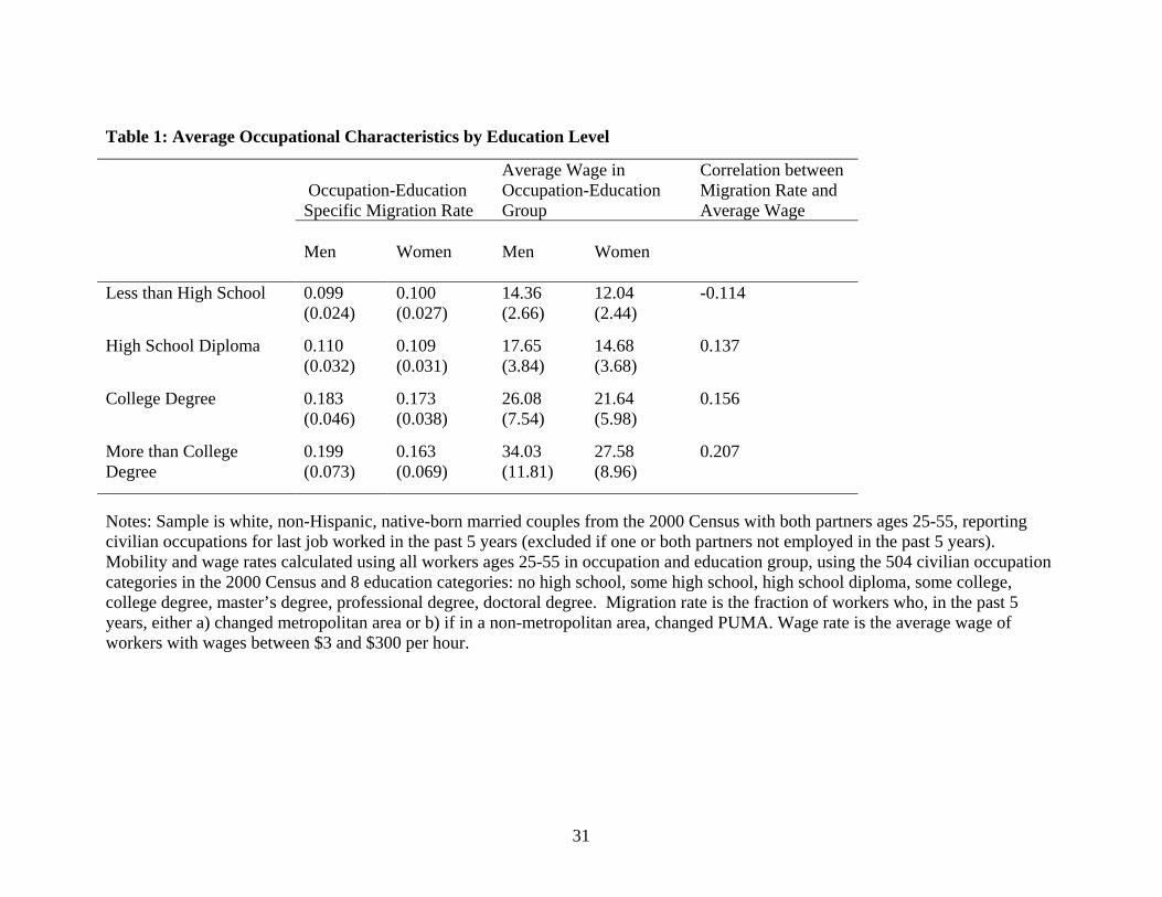
Table 1: Average Occupational Characteristics by Education Level
Occupation-Education Specific Migration Rate
Average Wage in Occupation-Education Group
Correlation between Migration Rate and Average Wage
Men
Women
Men
Women
Less than High School 0.099 (0.024)
0.100 (0.027)
14.36 (2.66)
12.04
-0.114 (2.44)
High School Diploma
0.110 (0.032)
0.109 (0.031)
17.65 (3.84)
14.68 (3.68)
0.137
College Degree 0.183 (0.046)
0.173 (0.038)
26.08 (7.54)
21.64
(5.98) 0.156
More than College Degree
0.199 (0.073)
0.163 (0.069)
34.03 (11.81)
27.58
(8.96)
0.207
Notes: Sample is white, non-Hispanic, native-born married couples from the 2000 Census with both partners ages 25-55, reporting civilian occupations for last job worked in the past 5 years (excluded if one or both partners not employed in the past 5 years). Mobility and wage rates calculated using all workers ages 25-55 in occupation and education group, using the 504 civilian occupation categories in the 2000 Census and 8 education categories: no high school, some high school, high school diploma, some college, college degree, master’s degree, professional degree, doctoral degree. Migration rate is the fraction of workers who, in the past 5 years, either a) changed metropolitan area or b) if in a non-metropolitan area, changed PUMA. Wage rate is the average wage of workers with wages between $3 and $300 per hour.
31
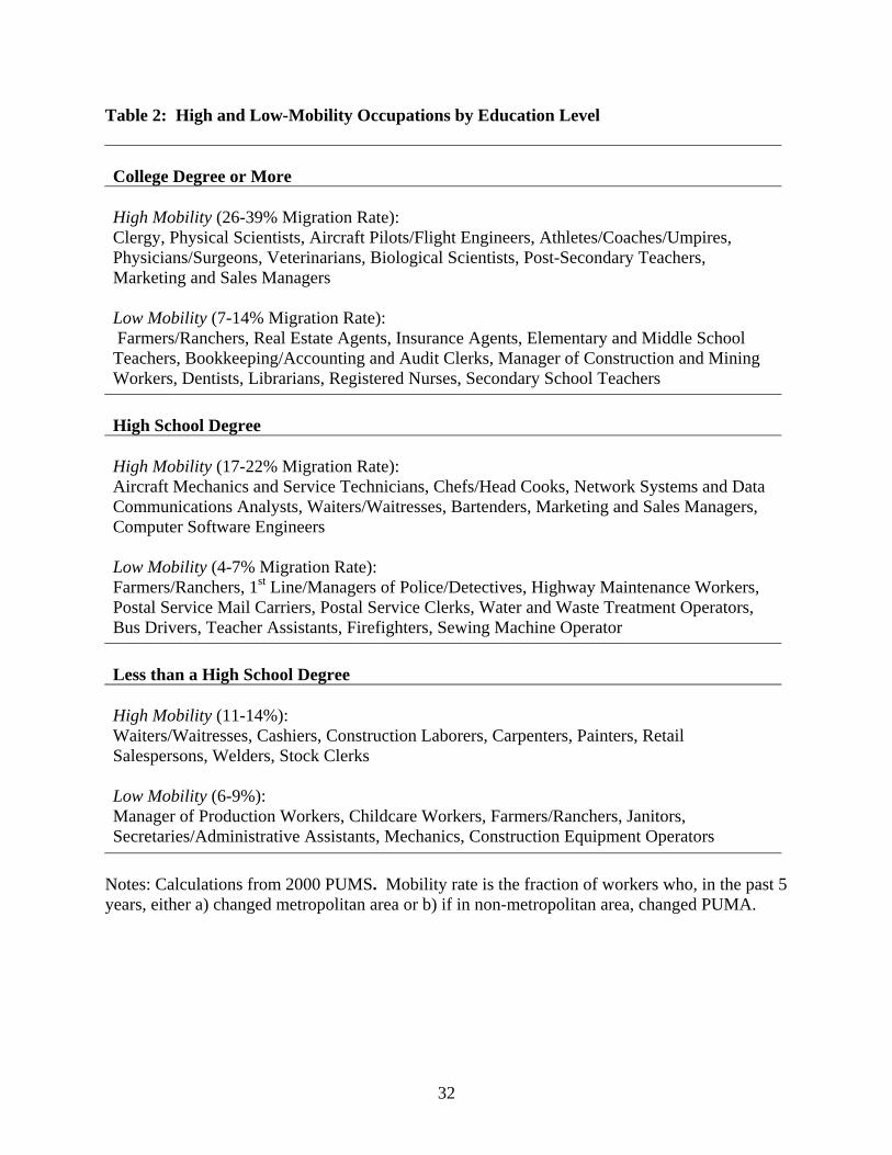
Table 2: High and Low-Mobility Occupations by Education Level College Degree or More High Mobility (26-39% Migration Rate): Clergy, Physical Scientists, Aircraft Pilots/Flight Engineers, Athletes/Coaches/Umpires, Physicians/Surgeons, Veterinarians, Biological Scientists, Post-Secondary Teachers, Marketing and Sales Managers Low Mobility (7-14% Migration Rate): Farmers/Ranchers, Real Estate Agents, Insurance Agents, Elementary and Middle School Teachers, Bookkeeping/Accounting and Audit Clerks, Manager of Construction and Mining Workers, Dentists, Librarians, Registered Nurses, Secondary School Teachers High School Degree High Mobility (17-22% Migration Rate): Aircraft Mechanics and Service Technicians, Chefs/Head Cooks, Network Systems and Data Communications Analysts, Waiters/Waitresses, Bartenders, Marketing and Sales Managers, Computer Software Engineers Low Mobility (4-7% Migration Rate): Farmers/Ranchers, 1st Line/Managers of Police/Detectives, Highway Maintenance Workers, Postal Service Mail Carriers, Postal Service Clerks, Water and Waste Treatment Operators, Bus Drivers, Teacher Assistants, Firefighters, Sewing Machine Operator Less than a High School Degree High Mobility (11-14%): Waiters/Waitresses, Cashiers, Construction Laborers, Carpenters, Painters, Retail Salespersons, Welders, Stock Clerks Low Mobility (6-9%): Manager of Production Workers, Childcare Workers, Farmers/Ranchers, Janitors, Secretaries/Administrative Assistants, Mechanics, Construction Equipment Operators
Notes: Calculations from 2000 PUMS. Mobility rate is the fraction of workers who, in the past 5 years, either a) changed metropolitan area or b) if in non-metropolitan area, changed PUMA.
32
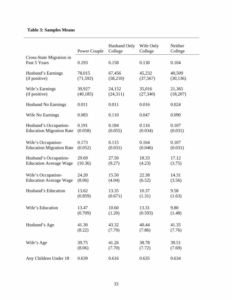
Table 3: Samples Means
Power Couple
Husband Only College
Wife Only College
Neither College
Cross-State Migration in Past 5 Years
0.193
0.158
0.130
0.104
Husband’s Earnings (if positive)
78,015 (71,592)
67,456 (58,210)
45,232 (37,567)
40,509 (30,136)
Wife’s Earnings (if positive)
39,927 (40,185)
24,152 (24,311)
35,016 (27,340)
21,365 (18,207)
Husband No Earnings
0.011 0.011 0.016 0.024
Wife No Earnings
0.083 0.110 0.047 0.090
Husband’s Occupation-Education Migration Rate
0.191 (0.058)
0.184 (0.055)
0.116 (0.034)
0.107 (0.031)
Wife’s Occupation-Education Migration Rate
0.173 (0.052)
0.115 (0.031)
0.164 (0.046)
0.107 (0.031)
Husband’s Occupation-Education Average Wage
29.69 (10.36)
27.50 (9.27)
18.33 (4.23)
17.12 (3.75)
Wife’s Occupation-Education Average Wage
24.20 (8.06)
15.50 (4.04)
22.38 (6.52)
14.31 (3.56)
Husband’s Education 13.62 (0.859)
13.35 (0.671)
10.37 (1.31)
9.58 (1.63)
Wife’s Education 13.47 (0.709)
10.60 (1.20)
13.31 (0.593)
9.80 (1.48)
Husband’s Age
41.30 (8.22)
43.32 (7.70)
40.44 (7.86)
41.35 (7.76)
Wife’s Age
39.75 (8.06)
41.26 (7.70)
38.78 (7.72)
39.51 (7.69)
Any Children Under 18
0.639
0.616 0.635 0.634
33
Any Children Under 6
0.319
0.235
0.314 0.233
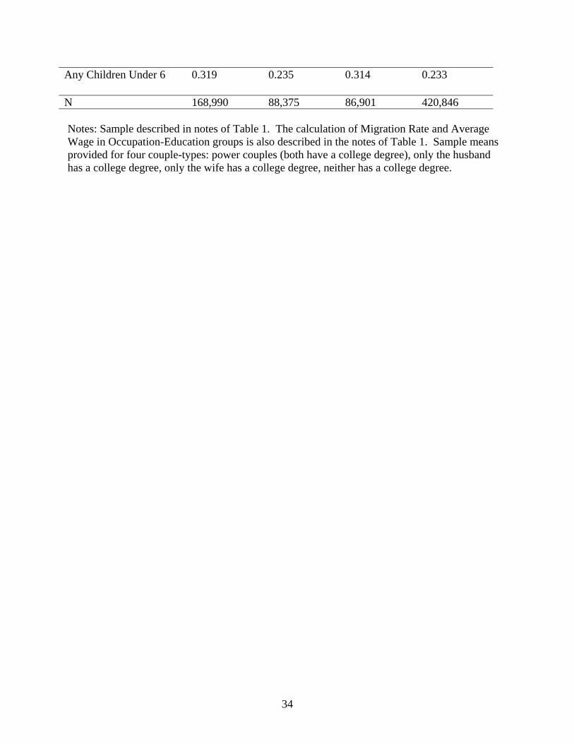
N 168,990 88,375 86,901 420,846 Notes: Sample described in notes of Table 1. The calculation of Migration Rate and Average Wage in Occupation-Education groups is also described in the notes of Table 1. Sample means provided for four couple-types: power couples (both have a college degree), only the husband has a college degree, only the wife has a college degree, neither has a college degree.
34
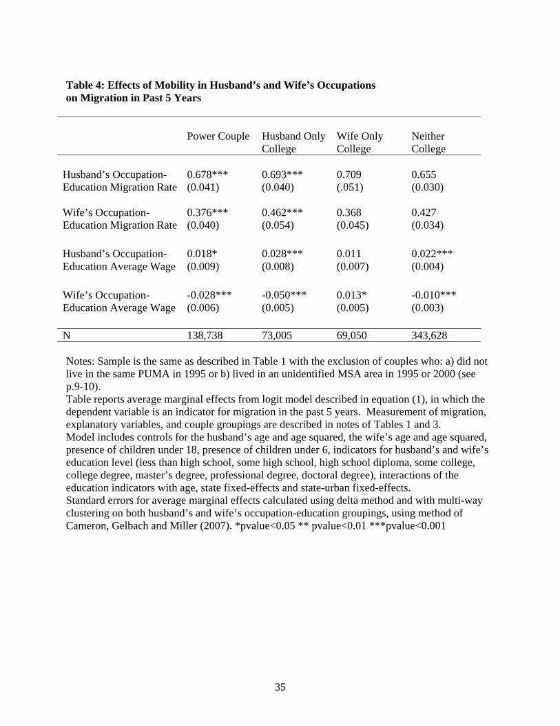
Table 4: Effects of Mobility in Husband’s and Wife’s Occupations on Migration in Past 5 Years
Power Couple
Husband Only College
Wife Only College
Neither College
Husband’s Occupation-Education Migration Rate
0.678*** (0.041)
0.693*** (0.040)
0.709 (.051)
0.655 (0.030)
Wife’s Occupation-Education Migration Rate
0.376*** (0.040)
0.462*** (0.054)
0.368 (0.045)
0.427 (0.034)
Husband’s Occupation-Education Average Wage
0.018* (0.009)
0.028*** (0.008)
0.011 (0.007)
0.022*** (0.004)
Wife’s Occupation-Education Average Wage
-0.028*** (0.006)
-0.050*** (0.005)
0.013* (0.005)
-0.010*** (0.003)
N 138,738 73,005 69,050 343,628 Notes: Sample is the same as described in Table 1 with the exclusion of couples who: a) did not live in the same PUMA in 1995 or b) lived in an unidentified MSA area in 1995 or 2000 (see p.9-10). Table reports average marginal effects from logit model described in equation (1), in which the dependent variable is an indicator for migration in the past 5 years. Measurement of migration, explanatory variables, and couple groupings are described in notes of Tables 1 and 3. Model includes controls for the husband’s age and age squared, the wife’s age and age squared, presence of children under 18, presence of children under 6, indicators for husband’s and wife’s education level (less than high school, some high school, high school diploma, some college, college degree, master’s degree, professional degree, doctoral degree), interactions of the education indicators with age, state fixed-effects and state-urban fixed-effects. Standard errors for average marginal effects calculated using delta method and with multi-way clustering on both husband’s and wife’s occupation-education groupings, using method of Cameron, Gelbach and Miller (2007). *pvalue<0.05 ** pvalue<0.01 ***pvalue<0.001
35
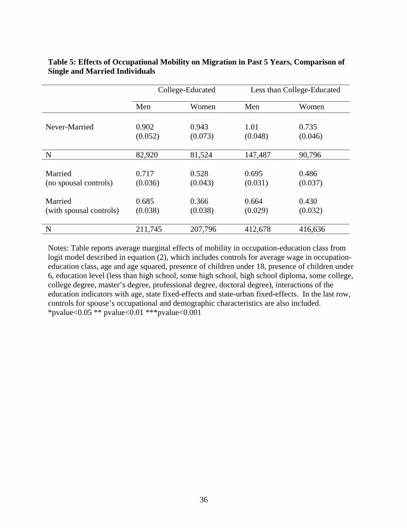
Table 5: Effects of Occupational Mobility on Migration in Past 5 Years, Comparison of Single and Married Individuals
College-Educated Less than College-Educated Men Women Men Women Never-Married
0.902 (0.052)
0.943 (0.073)
1.01 (0.048)
0.735 (0.046)
N 82,920 81,524 147,487 90,796 Married (no spousal controls)
0.717 (0.036)
0.528 (0.043)
0.695 (0.031)
0.486 (0.037)
Married (with spousal controls)
0.685 (0.038)
0.366 (0.038)
0.664 (0.029)
0.430 (0.032)
N 211,745 207,796 412,678 416,636 Notes: Table reports average marginal effects of mobility in occupation-education class from logit model described in equation (2), which includes controls for average wage in occupation-education class, age and age squared, presence of children under 18, presence of children under 6, education level (less than high school, some high school, high school diploma, some college, college degree, master’s degree, professional degree, doctoral degree), interactions of the education indicators with age, state fixed-effects and state-urban fixed-effects. In the last row, controls for spouse’s occupational and demographic characteristics are also included. *pvalue<0.05 ** pvalue<0.01 ***pvalue<0.001
36
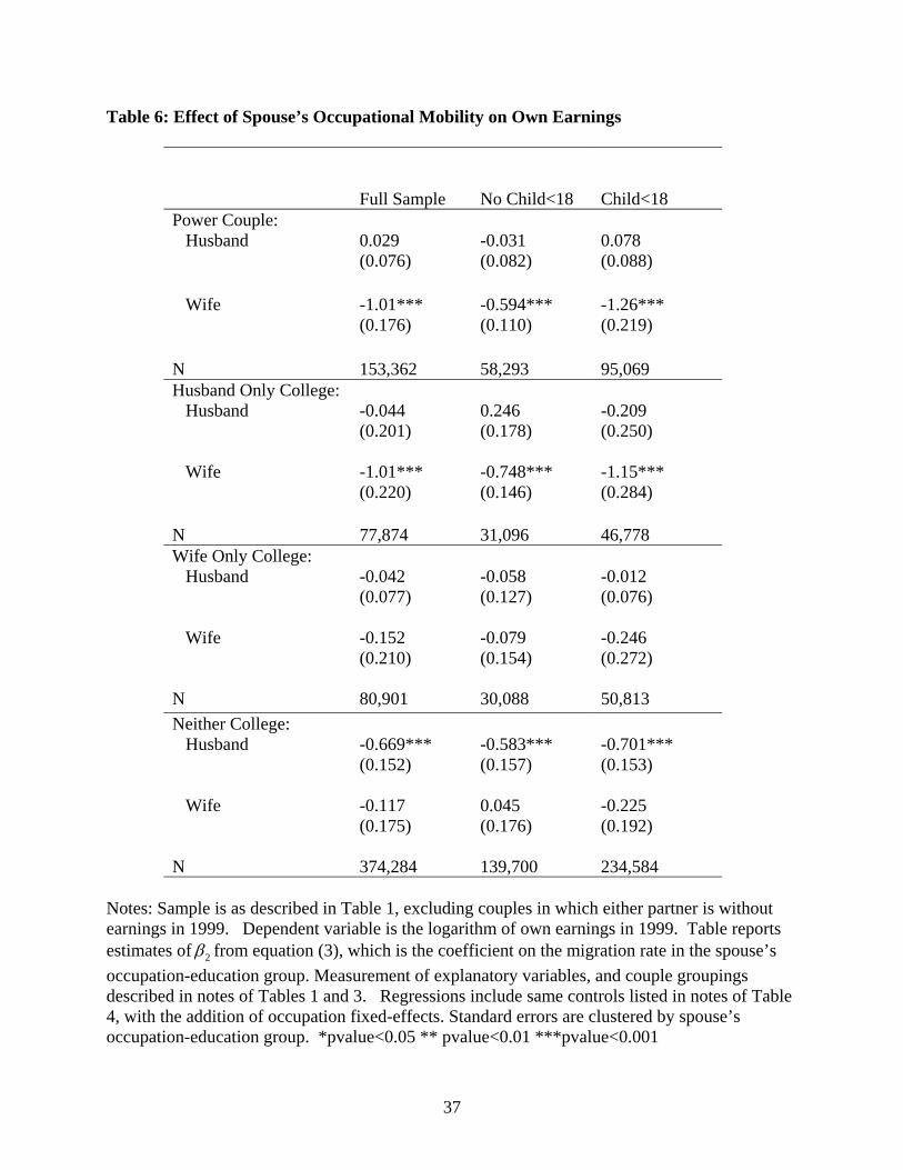
Table 6: Effect of Spouse’s Occupational Mobility on Own Earnings
Full Sample
No Child<18
Child<18
Power Couple: Husband
0.029 (0.076)
-0.031 (0.082)
0.078 (0.088)
Wife -1.01*** (0.176)
-0.594*** (0.110)
-1.26*** (0.219)
N 153,362 58,293 95,069 Husband Only College: Husband
-0.044 (0.201)
0.246 (0.178)
-0.209 (0.250)
Wife -1.01*** (0.220)
-0.748*** (0.146)
-1.15*** (0.284)
N 77,874 31,096 46,778 Wife Only College: Husband
-0.042 (0.077)
-0.058 (0.127)
-0.012 (0.076)
Wife
-0.152 (0.210)
-0.079 (0.154)
-0.246 (0.272)
N 80,901 30,088 50,813 Neither College: Husband
-0.669*** (0.152)
-0.583*** (0.157)
-0.701*** (0.153)
Wife
-0.117 (0.175)
0.045 (0.176)
-0.225 (0.192)
N 374,284 139,700 234,584 Notes: Sample is as described in Table 1, excluding couples in which either partner is without earnings in 1999. Dependent variable is the logarithm of own earnings in 1999. Table reports estimates of 2β from equation (3), which is the coefficient on the migration rate in the spouse’s occupation-education group. Measurement of explanatory variables, and couple groupings described in notes of Tables 1 and 3. Regressions include same controls listed in notes of Table 4, with the addition of occupation fixed-effects. Standard errors are clustered by spouse’s occupation-education group. *pvalue<0.05 ** pvalue<0.01 ***pvalue<0.001
37

Table 7: Effect of Spouse’s Occupational Mobility on Own Earnings, Super Power Couples
Full Sample
No Child<18
Child<18
Super Power Couple: Husband
-0.157 (0.097)
-0.197 (0.129)
-0.114 (0.111)
Wife -1.16*** (0.167)
-0.753*** (0.148)
-1.40*** (0.193)
N 32,368 12,303 20,065 Husband Only Advanced Degree: Husband
0.206 (0.149)
0.169 (0.232)
0.266 (0.183)
Wife -1.36*** (0.207)
-0.597*** (0.157)
-1.78*** (0.237)
N 30,791 11,294 19,497 Wife Only Advanced Degree: Husband
0.036 (0.105)
0.089 (0.105)
0.030 (0.142)
Wife
-0.408* (0.174)
-0.212 (0.166)
-0.581** (0.216)
N 25,151 10,275 14,876 Notes: Sample restricted to the dual-earner power couples used in the first row of Table 6. Super power couples are those in which both members have an advanced degree (master’s, professional or doctorate). Model is the same earnings regression estimated in Table 6. Standard errors are clustered by spouse’s occupation-education group. *pvalue<0.05 ** pvalue<0.01 ***pvalue<0.001
38
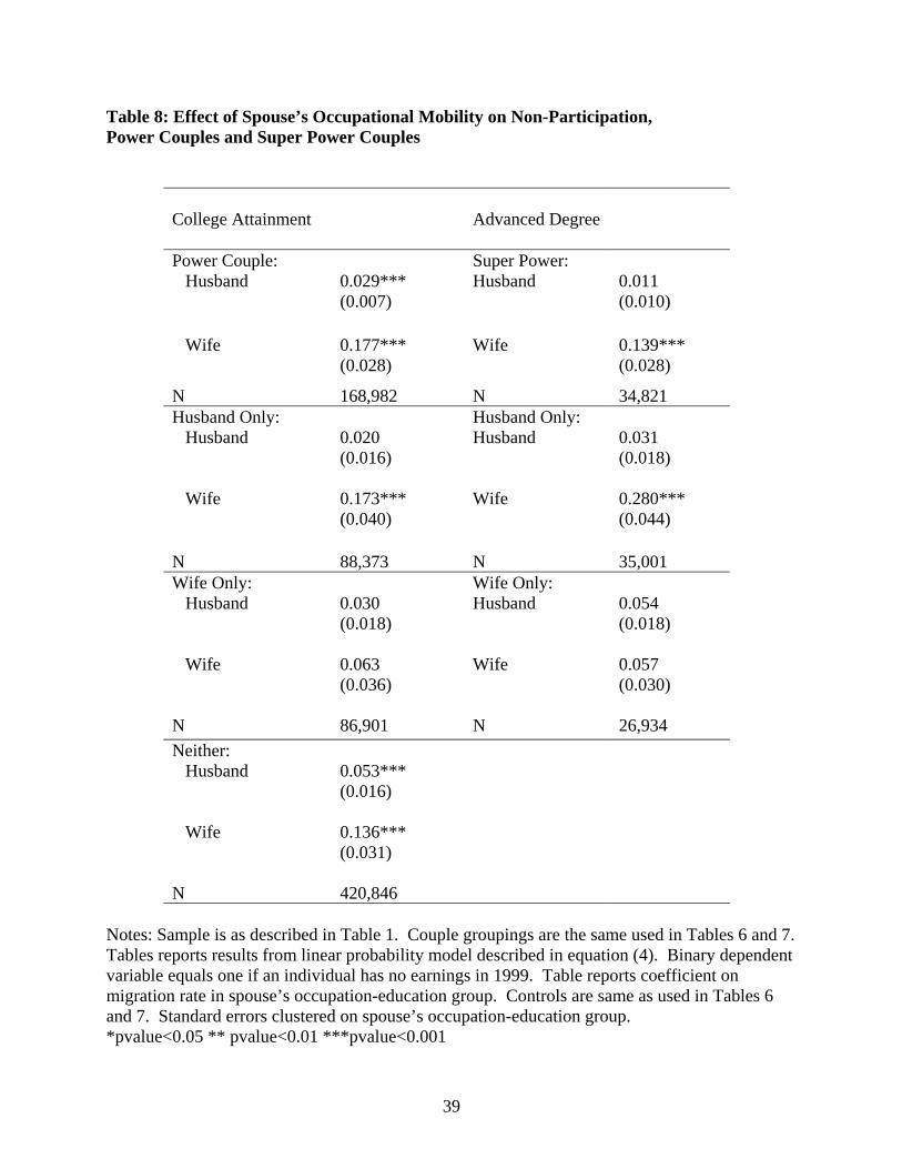
Table 8: Effect of Spouse’s Occupational Mobility on Non-Participation, Power Couples and Super Power Couples
College Attainment
Advanced Degree
Power Couple: Husband
0.029*** (0.007)
Super Power: Husband
0.011 (0.010)
Wife 0.177*** (0.028)
Wife 0.139*** (0.028)
N 168,982 N 34,821 Husband Only: Husband
0.020 (0.016)
Husband Only: Husband
0.031 (0.018)
Wife 0.173*** (0.040)
Wife 0.280*** (0.044)
N 88,373 N 35,001 Wife Only: Husband
0.030 (0.018)
Wife Only: Husband
0.054 (0.018)
Wife
0.063 (0.036)
Wife 0.057 (0.030)
N 86,901 N 26,934 Neither: Husband
0.053*** (0.016)
Wife
0.136*** (0.031)
N 420,846 Notes: Sample is as described in Table 1. Couple groupings are the same used in Tables 6 and 7. Tables reports results from linear probability model described in equation (4). Binary dependent variable equals one if an individual has no earnings in 1999. Table reports coefficient on migration rate in spouse’s occupation-education group. Controls are same as used in Tables 6 and 7. Standard errors clustered on spouse’s occupation-education group. *pvalue<0.05 ** pvalue<0.01 ***pvalue<0.001
39
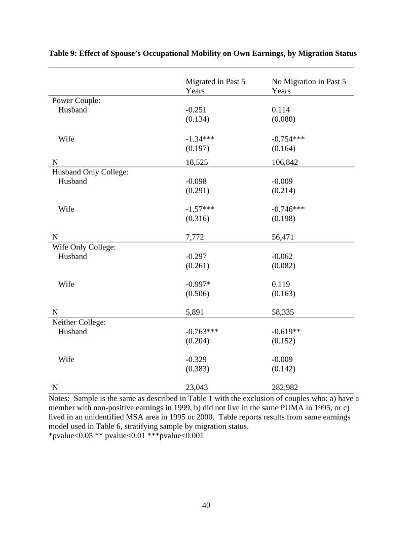
Table 9: Effect of Spouse’s Occupational Mobility on Own Earnings, by Migration Status
Migrated in Past 5 Years
No Migration in Past 5 Years
Power Couple: Husband
-0.251 (0.134)
0.114 (0.080)
Wife -1.34*** (0.197)
-0.754*** (0.164)
N 18,525 106,842 Husband Only College: Husband
-0.098 (0.291)
-0.009 (0.214)
Wife
-1.57*** (0.316)
-0.746*** (0.198)
N 7,772 56,471 Wife Only College: Husband
-0.297 (0.261)
-0.062 (0.082)
Wife
-0.997* (0.506)
0.119 (0.163)
N 5,891 58,335 Neither College: Husband
-0.763*** (0.204)
-0.619** (0.152)
Wife
-0.329 (0.383)
-0.009 (0.142)
N 23,043 282,982 Notes: Sample is the same as described in Table 1 with the exclusion of couples who: a) have a member with non-positive earnings in 1999, b) did not live in the same PUMA in 1995, or c) lived in an unidentified MSA area in 1995 or 2000. Table reports results from same earnings model used in Table 6, stratifying sample by migration status. *pvalue<0.05 ** pvalue<0.01 ***pvalue<0.001
40