Embed Size (px)
Citation preview

Spot-Weld Fatigue Optimization
FILIP ANDERSSON
RHODEL BENGTSSON
KTH ROYAL INSTITUTE OF TECHNOLOGYSCHOOL OF ENGINEERING SCIENCES
DEGREE PROJECT IN MECHANICAL ENGINEERINGAND MATERIALS DESIGN, SECOND CYCLE,30 CREDITSSTOCKHOLM, SWEDEN 2018

ROYAL INSTITUTE OF TECHNOLOGY
MASTER THESIS
Spot-Weld Fatigue Optimization
Authors:Filip AnderssonRhodel Bengtsson
Supervisor:Ann-Britt Ryberg
A thesis submitted in fulfillment of the requirementsfor the degree of Master of Science in Engineering
in the
Solid Mechanics Department
June 7, 2018

ii
“If we knew what we were doing, it wouldn’t be called research”
Albert Einstein
iii
AbstractThe purpose of this thesis project is to develop a methodology that can be used tominimize the number of spot-welds in a mechanical structure, this is done in a re-liable manner via optimization methods. The optimization considers fatigue life inspot-welds and also stiffness and eigenfrequency values. The first chapter of thisthesis presents a spot-weld fatigue model proposed by Rupp (1995), common FE-models of spot-welds and also important aspects about structural optimization ingeneral. The second chapter further describes how topology optimization and size(parameter) optimization are applied on a simple multi-weld model with respect tothe aforementioned structural constraints. The topology optimization is later usedon a full-size car model, while the size optimization is used to optimize the multi-weld model by adding an non-linear structural constraint - a crash indentation con-straint. The spot-weld fatigue model proposed by Rupp (1995), is also verified bycomparing FE results using different FE-models of spot-welds compared to fatiguedata by Long and Khanna (2007). Both optimization methods successfully mini-mize the total amount of spot-welds on the multi-weld model. The topology opti-mization, accompanied with the gradient based MFD algorithm, minimizes the totalspot-welds with around 15% and 3% on the multi-weld model and car body respec-tively. The size optimization, using design of experiments and response surfaces,manages to reduce the number of welds in the multi-weld model by 25%. However,with the size optimization the computational time is several orders of magnitudelonger - even without the formulation of the crash constraint. The fatigue spot-weldmodel fares reasonably well compared to the experimental fatigue data, regardlessof the FE model of the spot-weld. It is concluded that the ACM model would berecommended based on its compatibility with fatigue and optimization methods,mesh-independence and also other studies have shown its ability to represent stiff-ness and eigenfrequency correctly.
Keywords: Spot-weld, Fatigue, ACM, CWELD, Topology Optimization, Size Opti-mization, Response Surface, DOE, Genetic Algorithm, Most Feasible Direction, MFD
(1995), is also verified by comparing FE results using different FE-models of spot-welds compared to fatigue data by Long and Khanna (2007). Both optimizationmethods successfully minimized the total amount of spot-welds on the multi-weldmodel. The topology optimization, accompanied with the gradient based MFD algo-rithm, minimized the total spot-welds with around 15% and 3% on the multi-weldmodel and car body respectively. The size optimization, using design of experimentsand response surfaces, managed to reduce the number of welds in the multi-weldmodel by 25%. However, with the size optimization it took orders of magnitudelonger time to compute the results - even without the formulation of the crash con-straint. The fatigue spot-weld model fared reasonably well compared to the ex-perimentally.a, oberoende av FE-modell på punktsvetsarna. ACM-modellen rekom-menderas på grund av dess kompatibilitet med utmattning och optimeringsmetodersamt att andra studier har visat dess förmåga att representera styvhet och egen-frekvens.llllllllllllllllllllllllllllllllllllllllllllllllllllllllllllllllllllllllllllllllllllll
iv
ngsrikt den totala mängden punktsvetsar hos multisvetsmodellen. Topologi-optimeringen, tillsammans med den gradientbaserade MFD-algoritmen minimer-ade mängden med cirka 15% och 3% på multisvetsmodellen respektive bilkarossen.llllllllllllllllllllllllllllllllllllllllllllllllllllllllllllllllllllllllllllllllllllllllllllllllllllllllllllllllllllllllllllllllllllllllllllllllllllllllllllllllllllllllllllllllllllllll
SammanfattningMålet med detta examensprojekt är att ta fram en metodik som kan användas dåantalet punktsvetsar minimeras i en mekanisk struktur, detta ska göras på ett tillför-litligt sätt via optimeringsmetoder. Optimeringen ska ta hänsyn till utmattning ipunktsvetsarna men också styvhet och egenfrekvensvärde. Första kapitlet i dennaavhandling presenterar en utmattningsmodell för punktsvetsar som föreslås av Rupp(1995), vanligt förkomna FE-modeller av punktsvetsar samt viktiga aspekter av struk-turell optimering i allmänhet. Det andra kapitlet beskriver vidare hur topologi-optimering och parameter-optimering tillämpas på en enkel multisvets modell medhänsyn till de ovannämnda strukturella bivillkoren. Topologi-optimeringen användssedan på en fullskalig bilmodell, parameter-optimeringen används istället för att op-timera multisvetsmodellen med hänsyn till ett krock-lastfall. Utmattningsmodellensom har föreslagits av Rupp (1995), verifieras också genom att jämföra FE-resultatmed olika FE-modeller av punktsvetsar jämfört med utmattningsdata av Long andKhanna (2007). Båda optimeringsmetoderna minskade framgångsrikt den totalamängden punktsvetsar hos multisvetsmodellen. Topologi-optimeringen, tillsam-mans med den gradientbaserade MFD-algoritmen minimerade mängden med cirka15% och 3% på multisvetsmodellen respektive bilkarossen. Parameter-optimeringen,tillsammans med användandet av DOE och responsytor, lyckades minska antaletmed 25 % på multisvetsmodellen men det tog flera storleksordningar längre tidför att beräkna resultatet - oavsett om man inkluderade krockproblemet eller inte.Utmattningsmodellen uppträdde relativt bra jämfört med data, oberoende av FE-modell på punktsvetsarna. ACM-modellen rekommenderas på grund av dess kom-patibilitet med utmattning och optimeringsmetoder, mesh oberoende samt att andrastudier har visat dess goda förmåga att representera styvhet och egenfrekvens.

v
AcknowledgementsWe would like to express our appreciation to Dr. Ann-Britt Ryberg for her guidanceduring the term of our thesis. Without her help and counsel, always generouslyand unstintingly given, the completion of this work would have been immeasur-ably more difficult.
We are also indebted to the company of Combitech and their staff for their supportand granting us access to their resources. The constant association with the mem-bers of Combitech CAE groups has been most pleasurable.
Finally, we would like to thank the staff of Altair, especially Ms. Britta Käck forimparting her knowledge and expertise during our work.
vi
Contents
Abstract iii
Acknowledgements v
1 Introduction 1
1.1 Objective . . . . . . . . . . . . . . . . . . . . . . . . . . . . . . . . . . . . 2
1.2 Delimiter . . . . . . . . . . . . . . . . . . . . . . . . . . . . . . . . . . . . 2
1.3 Fatigue Theory . . . . . . . . . . . . . . . . . . . . . . . . . . . . . . . . 2
1.3.1 Variable and Constant Load Amplitude . . . . . . . . . . . . . . 31.3.2 Approach to Spot-Weld Fatigue . . . . . . . . . . . . . . . . . . . 4
1.4 Finite Element Spot-Welds . . . . . . . . . . . . . . . . . . . . . . . . . . 7
1.4.1 P2P . . . . . . . . . . . . . . . . . . . . . . . . . . . . . . . . . . . 81.4.2 ACM . . . . . . . . . . . . . . . . . . . . . . . . . . . . . . . . . . 81.4.3 CWELD . . . . . . . . . . . . . . . . . . . . . . . . . . . . . . . . 9
1.5 Structural Optimization . . . . . . . . . . . . . . . . . . . . . . . . . . . 10
1.5.1 Pitfalls and Possibilities of Optimization Problems . . . . . . . . 111.5.2 Topology Optimization . . . . . . . . . . . . . . . . . . . . . . . 121.5.3 Size Optimization with Response Surfaces and Genetic Algo-
rithms . . . . . . . . . . . . . . . . . . . . . . . . . . . . . . . . . 151.6 Previous Works on Optimization and Spot-Welds . . . . . . . . . . . . 19
1.6.1 Topology Optimization and Spot-Welds . . . . . . . . . . . . . . 191.6.2 Size Optimization and Spot-Welds . . . . . . . . . . . . . . . . . 20
2 Method 23
2.1 Verification of Rupp’s approach and comparison of weld model types . 24
2.2 Multi-Weld Model . . . . . . . . . . . . . . . . . . . . . . . . . . . . . . . 27
2.3 Topology Optimization Setup . . . . . . . . . . . . . . . . . . . . . . . . 29
2.4 Size Optimization Setup . . . . . . . . . . . . . . . . . . . . . . . . . . . 31
2.5 Comparison of Optimization Techniques . . . . . . . . . . . . . . . . . 34
2.6 Final Application . . . . . . . . . . . . . . . . . . . . . . . . . . . . . . . 34
3 Results 37
3.1 Fatigue verification results . . . . . . . . . . . . . . . . . . . . . . . . . . 37
3.2 Optimization Results . . . . . . . . . . . . . . . . . . . . . . . . . . . . . 42
vii
3.2.1 Topology Optimization Results . . . . . . . . . . . . . . . . . . . 443.2.2 Size Optimization Results . . . . . . . . . . . . . . . . . . . . . . 47
3.3 Comparison of optimization results . . . . . . . . . . . . . . . . . . . . . 51
3.4 Final Application . . . . . . . . . . . . . . . . . . . . . . . . . . . . . . . 51
4 Discussion 53
4.1 Regarding the Fatigue Results . . . . . . . . . . . . . . . . . . . . . . . . 53
4.2 Regarding the Optimization Results . . . . . . . . . . . . . . . . . . . . 54
4.3 Further Work . . . . . . . . . . . . . . . . . . . . . . . . . . . . . . . . . 58
5 Conclusion 59
Bibliography 61
viii
List of Figures
1.1 Schematic description of RSW process (Pan, 2010) . . . . . . . . . . . . 11.2 Rainflow counting example (Matsuishi and Endo, 1968). . . . . . . . . 31.3 Circular plate model for sheet metals (Kang, 2000). . . . . . . . . . . . . 51.4 Schematics of how t, θ and d relates to problem in question. In this
figure, only the mid-plane of the sheets are shown (NCode TheoryManual). . . . . . . . . . . . . . . . . . . . . . . . . . . . . . . . . . . . . 5
1.5 Beam model for nugget subjected to tension, bending and shear (Kang,2000). . . . . . . . . . . . . . . . . . . . . . . . . . . . . . . . . . . . . . . 6
1.6 Spot weld analysis process summary with time, T. . . . . . . . . . . . . 71.7 Schematic description of the P2P model (Andersson and Deleskog,
2014). . . . . . . . . . . . . . . . . . . . . . . . . . . . . . . . . . . . . . . 81.8 Schematic description of the ACM model (Palmonella, 2005). . . . . . . 91.9 Schematic description of the CWELD model (Fang, 2011). . . . . . . . . 101.10 Example of a convex and non-convex (objective) function (Svanberg,
2017). . . . . . . . . . . . . . . . . . . . . . . . . . . . . . . . . . . . . . . 121.11 Simple sine function with infinitely many local optima. . . . . . . . . . 121.12 Impact on stiffness using different penalization factors p. . . . . . . . . 131.13 Example I and II shows how Monte Carlo and LHS method samples
respectively. . . . . . . . . . . . . . . . . . . . . . . . . . . . . . . . . . . 171.14 Flowchart of the GRSM optimization algorithm. . . . . . . . . . . . . . 181.15 Flowchart of the GA method. . . . . . . . . . . . . . . . . . . . . . . . . 191.16 Topology optimization model used by Puchner (2006) to redistribute
welds. . . . . . . . . . . . . . . . . . . . . . . . . . . . . . . . . . . . . . . 201.17 a ) distribution using stiffness b ) distribution using fatigue c ) damage
in individual welds along the weld line. . . . . . . . . . . . . . . . . . . 201.18 Spot-welding lines identified for the driver and passenger seats (d’Ippolito
et al., 2008). . . . . . . . . . . . . . . . . . . . . . . . . . . . . . . . . . . . 211.19 Parameterization of spot-weld locations in CAD-CAE Virtual.lab (d’Ippolito
et al., 2008). . . . . . . . . . . . . . . . . . . . . . . . . . . . . . . . . . . . 211.20 Simulated annealing algorithm for minimization problem (Abasi, 2012). 22
2.1 Flowchart of thesis project . . . . . . . . . . . . . . . . . . . . . . . . . . 242.2 Schematic description of single weld tensile shear (TS) specimen, di-
mensions in mm . . . . . . . . . . . . . . . . . . . . . . . . . . . . . . . . 252.3 Schematic description of single weld coach peel (CP) specimen, di-
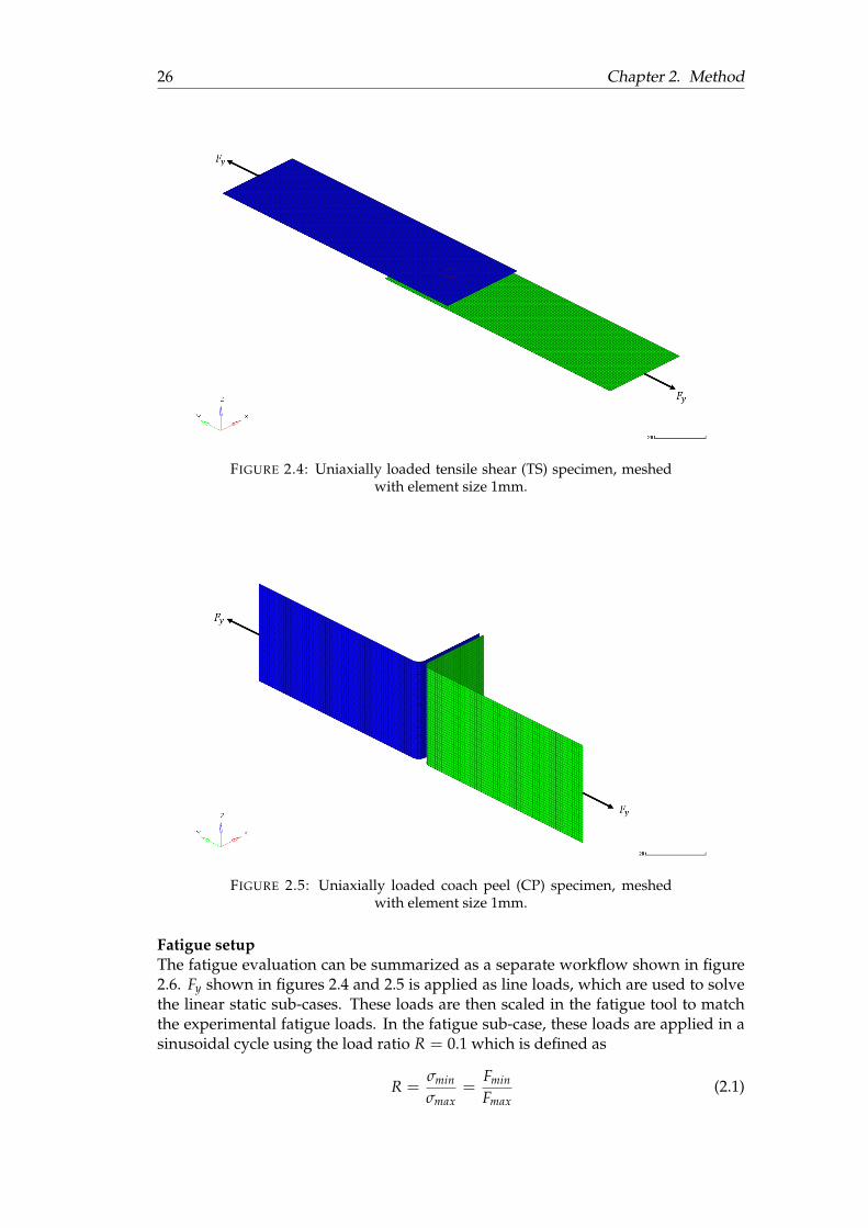
mensions in mm . . . . . . . . . . . . . . . . . . . . . . . . . . . . . . . . 252.4 Uniaxially loaded tensile shear (TS) specimen, meshed with element
size 1mm. . . . . . . . . . . . . . . . . . . . . . . . . . . . . . . . . . . . . 262.5 Uniaxially loaded coach peel (CP) specimen, meshed with element
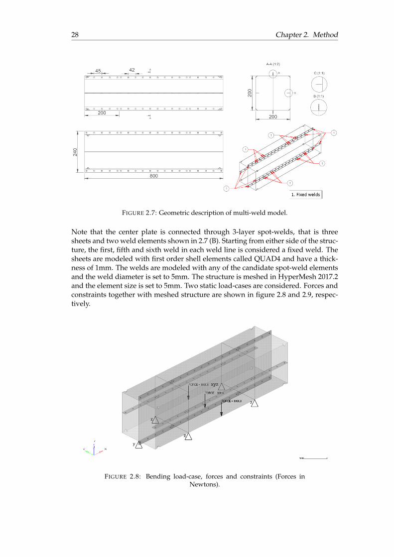
size 1mm. . . . . . . . . . . . . . . . . . . . . . . . . . . . . . . . . . . . . 262.6 Fatigue setup for benchmark structures . . . . . . . . . . . . . . . . . . 272.7 Geometric description of multi-weld model. . . . . . . . . . . . . . . . 28
ix
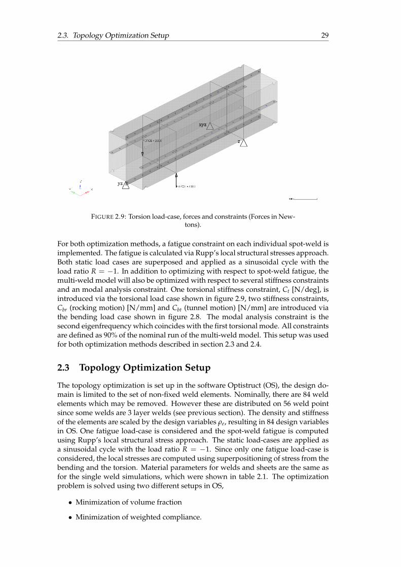
2.8 Bending load-case, forces and constraints (Forces in Newtons). . . . . . 282.9 Torsion load-case, forces and constraints (Forces in Newtons). . . . . . 292.10 Topology Optimization work-flow. . . . . . . . . . . . . . . . . . . . . . 312.11 The Multi-Weld model with 12 spot-weld lines. . . . . . . . . . . . . . . 322.12 A 100kg mass is applied with a speed of 15m/s on one end of the
multi-weld model, while constrained at the far end. d is the averagebeam length after the "crash", and of which the nominal value is 391.1mm . . . . . . . . . . . . . . . . . . . . . . . . . . . . . . . . . . . . . . . 33
2.13 Nominal weld distribution. . . . . . . . . . . . . . . . . . . . . . . . . . 342.14 a) global torsion b ) global bending c ) transverse bending front d )
longitudinal bending rear e ) modal analysis f ) rear belt pull. . . . . . . 35
3.1 The equivalent radial stresses on a single spot-weld subjected to sinu-soidal bending. . . . . . . . . . . . . . . . . . . . . . . . . . . . . . . . . 37
3.2 Benchmark test with CP specimen and element size 1mm. . . . . . . . 383.3 Benchmark test with CP specimen and element size 2mm. . . . . . . . 393.4 Benchmark test with CP specimen and element size 4mm. . . . . . . . 393.5 Benchmark test with TS specimen and element size 1mm. . . . . . . . . 403.6 Benchmark test with TS specimen and element size 2mm. . . . . . . . . 403.7 Benchmark test with TS specimen and element size 4mm. . . . . . . . . 413.8 Mesh density dependency CP specimen . . . . . . . . . . . . . . . . . . 413.9 Mesh density dependency TS specimen . . . . . . . . . . . . . . . . . . 423.10 Optimized Spot-Weld configuration using minimization of volume
and fatigue life constraint. . . . . . . . . . . . . . . . . . . . . . . . . . . 443.11 Optimized Spot-Weld configuration using minimization of weighted
compliance and fatigue life constraint. . . . . . . . . . . . . . . . . . . . 453.12 Optimized Spot-Weld configuration using minimization of volume
fraction and all linear constraints. . . . . . . . . . . . . . . . . . . . . . . 463.13 Optimized Spot-Weld configuration using minimization of weighted
compliance and all linear constraints. . . . . . . . . . . . . . . . . . . . . 473.14 Optimized Spot-Weld configurations with GRSM and GA method and
only using the fatigue constraint . . . . . . . . . . . . . . . . . . . . . . 483.15 Optimized Spot-Weld configuration with GRSM and GA and all linear
constraints. . . . . . . . . . . . . . . . . . . . . . . . . . . . . . . . . . . . 483.16 Optimized Spot-Weld configurations with GRSM and GA method and
using all linear constraints and crash constraint . . . . . . . . . . . . . . 493.17 a ) welds removed using only fatigue constraint b ) welds removed
using all linear constraints. . . . . . . . . . . . . . . . . . . . . . . . . . . 52
x
List of Tables
2.1 Material data for Weld nugget and Plates . . . . . . . . . . . . . . . . . 272.2 Linear Constraints for BIW topology optimization. . . . . . . . . . . . . 35
3.1 Optimization objective and constraints . . . . . . . . . . . . . . . . . . . 433.2 Optimized Spot-Weld configuration using minimization of volume
and fatigue life constraint. . . . . . . . . . . . . . . . . . . . . . . . . . . 443.3 Optimized Spot-Weld configuration using minimization of weighted
compliance and fatigue life constraint. . . . . . . . . . . . . . . . . . . . 453.4 Optimized Spot-Weld configuration using minimization of volume
fraction and all linear constraints. . . . . . . . . . . . . . . . . . . . . . . 463.5 Optimized Spot-Weld configuration using minimization of weighted
compliance and all linear constraints. . . . . . . . . . . . . . . . . . . . . 473.6 Size Optimization results with only fatigue constraint. . . . . . . . . . . 473.7 The optimal spot-weld configuration (only fatigue constraint) . . . . . 483.8 Size optimization results with all linear constraints. . . . . . . . . . . . 483.9 The optimal spot-weld configuration (all linear constraints) for both
algorithms . . . . . . . . . . . . . . . . . . . . . . . . . . . . . . . . . . . 493.10 Size optimization results with all linear constraints + crash constraint . 493.11 Optimal spot-weld configuration (all linear + crash) for both algorithms 503.12 Responses of the suggested optimal design validated in the simula-
tion model . . . . . . . . . . . . . . . . . . . . . . . . . . . . . . . . . . . 503.13 Relative difference between the responses given from the response
surface (Kriging) and the actual simulated design point . . . . . . . . . 503.14 Diagnostics of different response surfaces in terms of R-Square. Based
on the fatigue response. . . . . . . . . . . . . . . . . . . . . . . . . . . . 513.15 Comparison of optimization results . . . . . . . . . . . . . . . . . . . . . 513.16 BIW topology optimization responses. . . . . . . . . . . . . . . . . . . . 523.17 BIW Topology Optimization result summary . . . . . . . . . . . . . . . 52
1
Chapter 1
Introduction
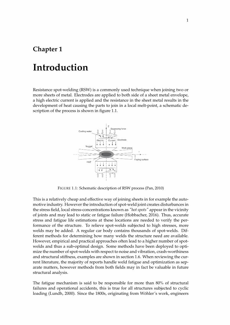
Resistance spot-welding (RSW) is a commonly used technique when joining two ormore sheets of metal. Electrodes are applied to both side of a sheet metal envelope,a high electric current is applied and the resistance in the sheet metal results in thedevelopment of heat causing the parts to join in a local melt-point, a schematic de-scription of the process is shown in figure 1.1.
FIGURE 1.1: Schematic description of RSW process (Pan, 2010)
This is a relatively cheap and effective way of joining sheets in for example the auto-motive industry. However the introduction of spot-weld joint creates disturbances inthe stress field, local stress-concentrations known as "hot spots" appear in the vicinityof joints and may lead to static or fatigue failure (Hobbacher, 2016). Thus, accuratestress and fatigue life estimations at these locations are needed to verify the per-formance of the structure. To relieve spot-welds subjected to high stresses, morewelds may be added. A regular car body contains thousands of spot-welds. Dif-ferent methods for determining how many welds the structure need are available.However, empirical and practical approaches often lead to a higher number of spot-welds and thus a sub-optimal design. Some methods have been deployed to opti-mize the number of spot-welds with respect to noise and vibration, crash-worthinessand structural stiffness, examples are shown in section 1.6. When reviewing the cur-rent literature, the majority of reports handle weld fatigue and optimization as sep-arate matters, however methods from both fields may in fact be valuable in futurestructural analysis.
The fatigue mechanism is said to be responsible for more than 80% of structuralfailures and operational accidents, this is true for all structures subjected to cyclicloading (Lundh, 2000). Since the 1800s, originating from Wöhler’s work, engineers
2 Chapter 1. Introduction
have developed methods on how to estimate the fatigue life of mechanical systemsto minimize the risk of said failures.
Reducing the number of welds, and thus the number of weld processes, may bea contributing factor when developing a time and cost-effective production. By theuse of reliable fatigue analysis combined with an optimized design, the performanceof the structure can be maintained.
1.1 Objective
Different methods have been developed to model mechanical structures containingwelds in order to analyze their complex geometry, load-distribution, material be-havior and failure. By applying and evaluating some of the current weld modelingmethods, the objective of this thesis is to identify a methodology which can be usedto accurately model spot-welds. This developed methodology will also combine thefields of fatigue analysis and structural optimization to reduce the number of spot-welds in a general mechanical structure, while maintaining key properties.
1.2 Delimiter
The methodology developed in this thesis work will focus on modeling techniqueand the combination and application of the fatigue and optimization theory. Thefatigue analysis will be limited to stress based damage computation and methodsincluding nominal stress approach and structural stress approach. The structuraloptimization is based on the topology and size optimization methods. Benchmarkstructures will be used to test, evaluate and compare both fatigue and optimizationresults. For the parallel but equally important aspects regarding welding techniquesand micro-mechanical behavior in and around the weld, we will refer to the worksof others. Models presented in this thesis will not fully capture the complexity ofthe spot-weld geometry nor the residual stresses and material behavior that are in-duced during the weld process. With that in mind, it will be shown that valuableconclusions can still be made using fatigue analysis and optimization methods incombination with welded structures.
1.3 Fatigue Theory
The fatigue phenomenon allows failure to happen even well below the ultimate ten-sile strength (Lundh, 2000). It has its basis from micro-cracks nucleating due to highstress concentrations from extremely small material and/or geometric defects. Thesecracks slowly propagates when the load varies cyclically in time. When the crack fi-nally reaches a critical size, a relatively low load is enough for failure to occur.
Fatigue can be classified into two types (Socie, 2017). High Cycle Fatigue (HCF) im-plies that the structure remains predominantly (macroscopically) elastic, resulting ina fatigue life above 104 cycles. Low Cycle Fatigue (LCF) implies that the structureremains predominantly (macroscopically) plastic, resulting in a fatigue life below104 cycles.
1.3. Fatigue Theory 3
In a controlled environment, fatigue testings can be done. Test specimens of thesame material and surface polish are uni-axially loaded cyclically in a purely alter-nating or pulsating manner. During testing, a number of specimens are loaded invarious magnitudes, and the number of cycles until failure are registered for eachmagnitude. The results are presented in an S-N diagram (Stress-Number diagram),where the stress amplitude, σA, of the specimens is plotted against its correspondinglogarithmic life, logN.
1.3.1 Variable and Constant Load Amplitude
The majority of fatigue testing is carried out at constant amplitude (CA), howevermechanical systems are often subjected to variable-amplitude (VA) loading in realapplications. There are a number of fatigue life prediction methods of structures in-volving VA load-histories. These differ from the methods used for CA load-historiesand the most widely used one is the Palmgren-Miner rule (Alfredsson, Larsson, andÖberg, 2017). The aforementioned method involves applying a load with stress am-plitude ∆Si onto the structure with ni cycles and calculate the total damage, D, as,
D =k
∑i=1
ni
Ni(1.1)
where k is the number of amplitudes during the load history and Ni is the corre-sponding fatigue life at ∆Si from a CA fatigue test. If damage is truly a linear processthe damage at failure will be equal to unity, however experiments have shown thisis not always the case. In simple two step block loading, a sequence of high ampli-tude cycles followed by low amplitude cycles will have a damage sum D < 1.0 atfailure. Similarly, a sequence of low amplitude cycles followed by high amplitudecycles may have a damage sum D > 1.0. Random loading histories have D ≈ 1.0.CA load histories obviously are D = 1.0, due to their inherent correlation with thePalmgren-Miner Rule.
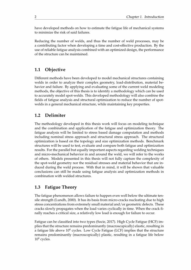
When observing a VA load-history, it can be difficult to distinguish the cycles andtheir corresponding amplitudes from each other. In 1968, the so called "Rainflow cy-cle counting" method was developed and it is a process to obtain equivalent constantamplitude cycles (Alfredsson, Larsson, and Öberg, 2017). Its name comes from theoriginal description from the Japanese researchers Matsuiski and Endo where theydescribe the process in terms of rain falling off a pagoda roof (Matsuishi and Endo,1968). By the use of rainflow counting the VA load history is translated to a series ofCA load cycles that can be used in equation 1.1. An example of rainflow counting isshown in figure 1.2.
FIGURE 1.2: Rainflow counting example (Matsuishi and Endo, 1968).
4 Chapter 1. Introduction
1.3.2 Approach to Spot-Weld Fatigue
Considering HCF fatigue in welds there are three main approaches when determin-ing fatigue life, nominal stress approach, fracture mechanic approach and structuralstress approach (Khanna, 2010). The nominal stress approach simply compute dam-age based on the stress calculated in the FE-elements, this approach will be appliedin this study. When applying the fracture mechanical approach initial cracks is as-sumed, different methods are then used to estimate the growth of those cracks. Thisapproach is not investigated in this thesis due to FE-software limitations, for moreinformation we refer to the works of Swellam (1991). The structural stress approachuses a equivalent structural stress for damage calculations, this is the main approachfor this thesis and is described below.
According to Rupp (1995), detailed stress FE-analyses at spot-welds are generallynot practical for automotive applications with respect to the corresponding com-puting expense. Instead, he reasoned that a nominal local structural stress directlyrelated to the loads carried by the spot-welded joint would be of more use in engi-neering. These analytical structural stresses are calculated based on beam and an-nular plate theory using the forces and moments transferred through the spot-weldseen as a beam element. For Rupp’s structural stress approach, two types of failuremodes of spot-welded joints are considered: cracking in the sheet metal and crack-ing through the weld nugget.
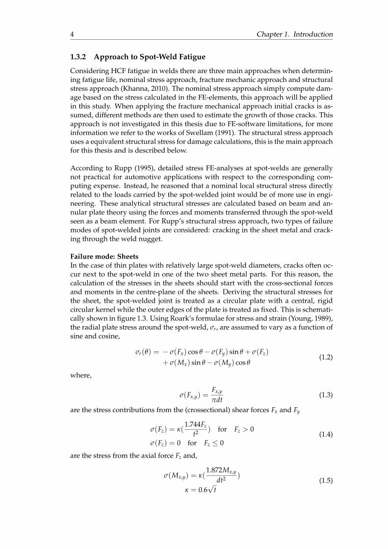
Failure mode: SheetsIn the case of thin plates with relatively large spot-weld diameters, cracks often oc-cur next to the spot-weld in one of the two sheet metal parts. For this reason, thecalculation of the stresses in the sheets should start with the cross-sectional forcesand moments in the centre-plane of the sheets. Deriving the structural stresses forthe sheet, the spot-welded joint is treated as a circular plate with a central, rigidcircular kernel while the outer edges of the plate is treated as fixed. This is schemati-cally shown in figure 1.3. Using Roark’s formulae for stress and strain (Young, 1989),the radial plate stress around the spot-weld, σr, are assumed to vary as a function ofsine and cosine,
σr(θ) = − σ(Fx) cos θ − σ(Fy) sin θ + σ(Fz)
+ σ(Mx) sin θ − σ(My) cos θ(1.2)
where,
σ(Fx,y) =Fx,y
πdt(1.3)
are the stress contributions from the (crossectional) shear forces Fx and Fy
σ(Fz) = κ(1.744Fz
t2 ) for Fz > 0
σ(Fz) = 0 for Fz ≤ 0(1.4)
are the stress from the axial force Fz and,
σ(Mx,y) = κ(1.872Mx,y
dt2 )
κ = 0.6√
t(1.5)
1.3. Fatigue Theory 5
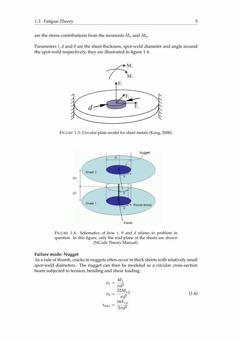
are the stress contributions from the moments Mx and My.
Parameters t, d and θ are the sheet thickness, spot-weld diameter and angle aroundthe spot-weld respectively, they are illustrated in figure 1.4.
FIGURE 1.3: Circular plate model for sheet metals (Kang, 2000).
FIGURE 1.4: Schematics of how t, θ and d relates to problem inquestion. In this figure, only the mid-plane of the sheets are shown
(NCode Theory Manual).
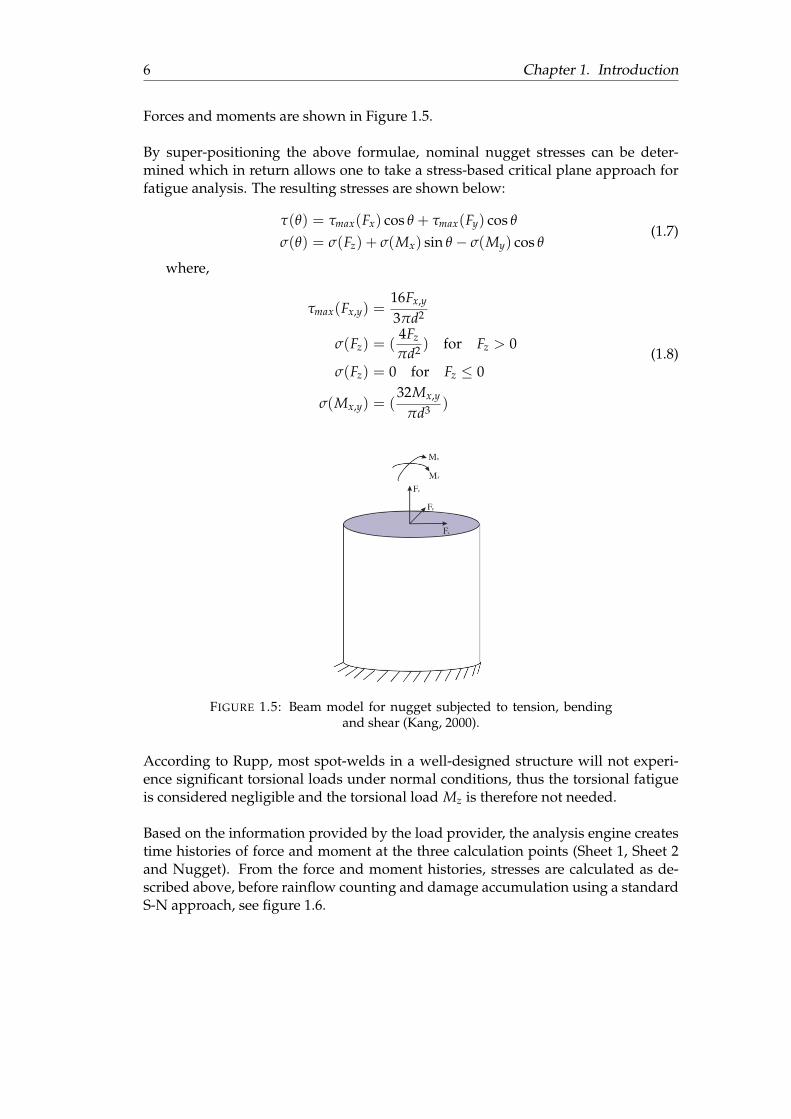
Failure mode: NuggetAs a rule of thumb, cracks in nuggets often occur in thick sheets with relatively smallspot-weld diameters. The nugget can then be modeled as a circular cross-sectionbeam subjected to tension, bending and shear loading.
σn =4Fz
πd2
σb =32Mx,y
πd3
τmax =16Fx,y
3πd2
(1.6)
6 Chapter 1. Introduction
Forces and moments are shown in Figure 1.5.
By super-positioning the above formulae, nominal nugget stresses can be deter-mined which in return allows one to take a stress-based critical plane approach forfatigue analysis. The resulting stresses are shown below:
τ(θ) = τmax(Fx) cos θ + τmax(Fy) cos θ
σ(θ) = σ(Fz) + σ(Mx) sin θ − σ(My) cos θ(1.7)
where,
τmax(Fx,y) =16Fx,y
3πd2
σ(Fz) = (4Fz
πd2 ) for Fz > 0
σ(Fz) = 0 for Fz ≤ 0
σ(Mx,y) = (32Mx,y
πd3 )
(1.8)
FIGURE 1.5: Beam model for nugget subjected to tension, bendingand shear (Kang, 2000).
According to Rupp, most spot-welds in a well-designed structure will not experi-ence significant torsional loads under normal conditions, thus the torsional fatigueis considered negligible and the torsional load Mz is therefore not needed.
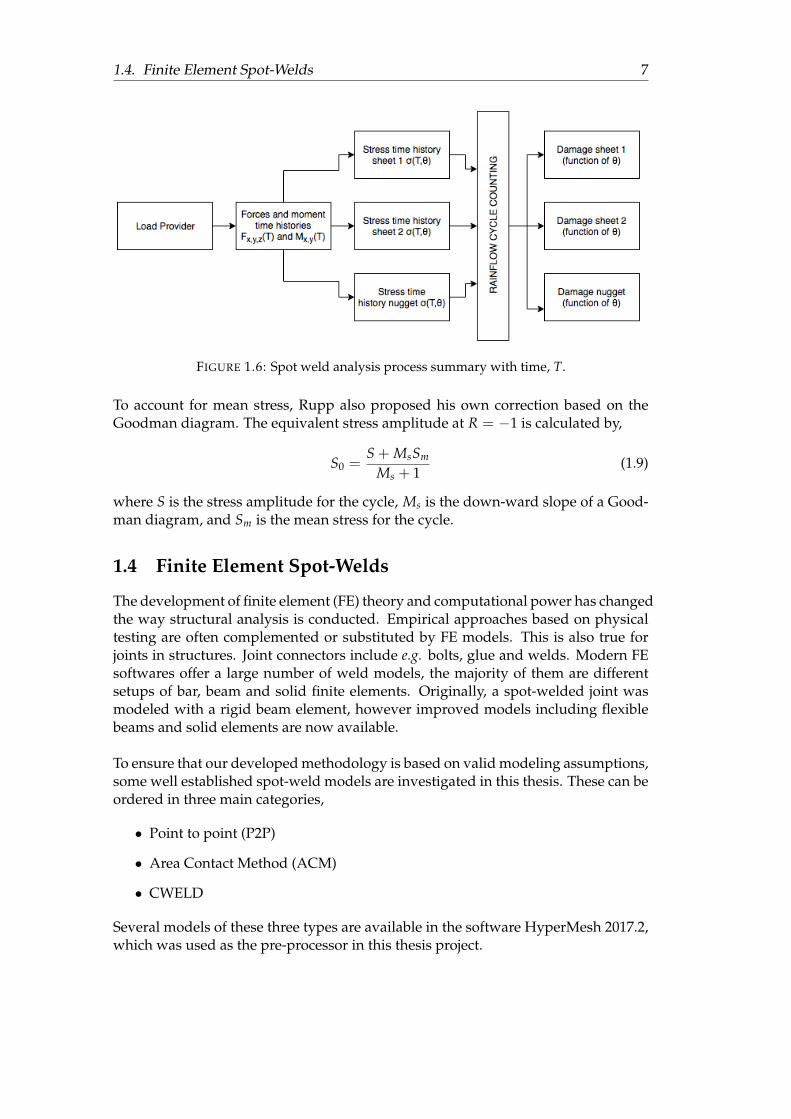
Based on the information provided by the load provider, the analysis engine createstime histories of force and moment at the three calculation points (Sheet 1, Sheet 2and Nugget). From the force and moment histories, stresses are calculated as de-scribed above, before rainflow counting and damage accumulation using a standardS-N approach, see figure 1.6.
1.4. Finite Element Spot-Welds 7
FIGURE 1.6: Spot weld analysis process summary with time, T.
To account for mean stress, Rupp also proposed his own correction based on theGoodman diagram. The equivalent stress amplitude at R = −1 is calculated by,
S0 =S + MsSm
Ms + 1(1.9)
where S is the stress amplitude for the cycle, Ms is the down-ward slope of a Good-man diagram, and Sm is the mean stress for the cycle.
1.4 Finite Element Spot-Welds
The development of finite element (FE) theory and computational power has changedthe way structural analysis is conducted. Empirical approaches based on physicaltesting are often complemented or substituted by FE models. This is also true forjoints in structures. Joint connectors include e.g. bolts, glue and welds. Modern FEsoftwares offer a large number of weld models, the majority of them are differentsetups of bar, beam and solid finite elements. Originally, a spot-welded joint wasmodeled with a rigid beam element, however improved models including flexiblebeams and solid elements are now available.
To ensure that our developed methodology is based on valid modeling assumptions,some well established spot-weld models are investigated in this thesis. These can beordered in three main categories,
• Point to point (P2P)
• Area Contact Method (ACM)
• CWELD
Several models of these three types are available in the software HyperMesh 2017.2,which was used as the pre-processor in this thesis project.
8 Chapter 1. Introduction
1.4.1 P2P
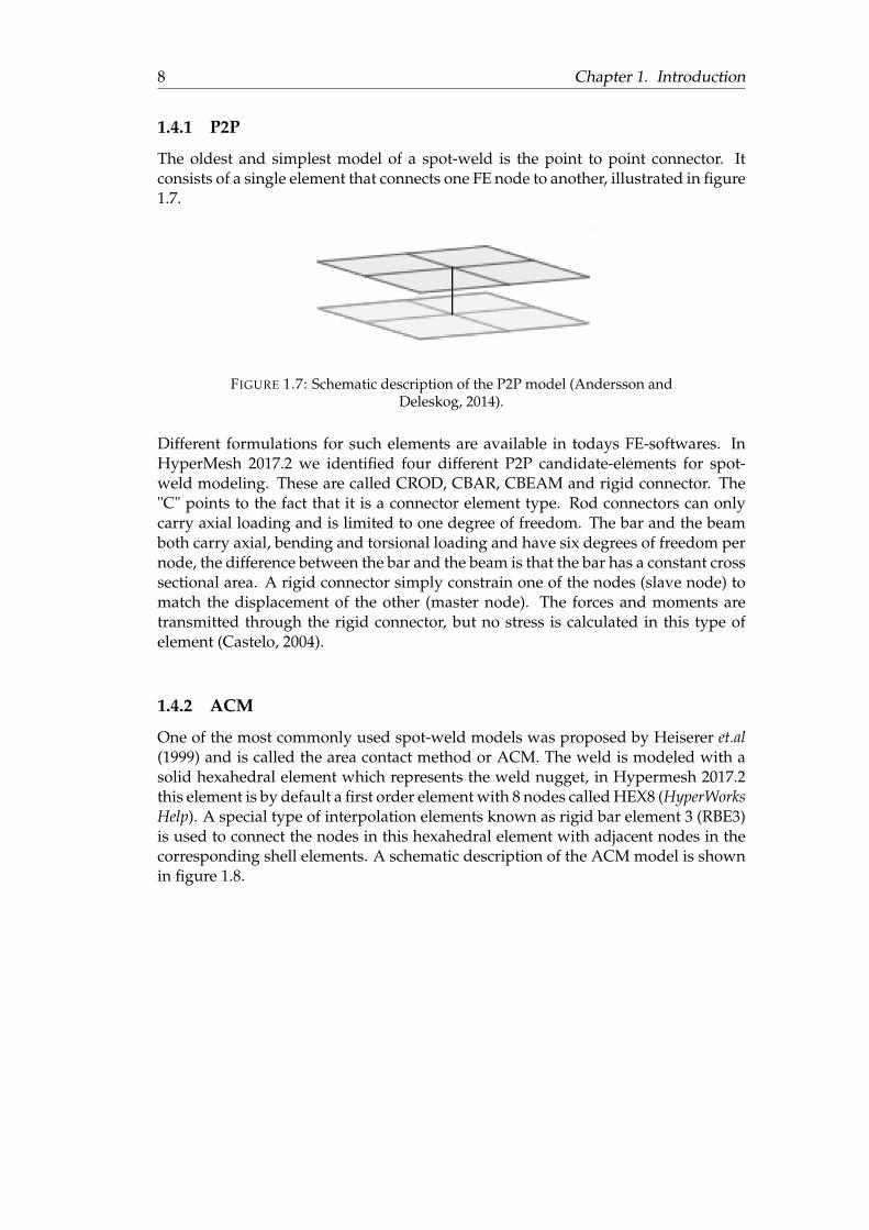
The oldest and simplest model of a spot-weld is the point to point connector. Itconsists of a single element that connects one FE node to another, illustrated in figure1.7.
FIGURE 1.7: Schematic description of the P2P model (Andersson andDeleskog, 2014).
Different formulations for such elements are available in todays FE-softwares. InHyperMesh 2017.2 we identified four different P2P candidate-elements for spot-weld modeling. These are called CROD, CBAR, CBEAM and rigid connector. The"C" points to the fact that it is a connector element type. Rod connectors can onlycarry axial loading and is limited to one degree of freedom. The bar and the beamboth carry axial, bending and torsional loading and have six degrees of freedom pernode, the difference between the bar and the beam is that the bar has a constant crosssectional area. A rigid connector simply constrain one of the nodes (slave node) tomatch the displacement of the other (master node). The forces and moments aretransmitted through the rigid connector, but no stress is calculated in this type ofelement (Castelo, 2004).
1.4.2 ACM
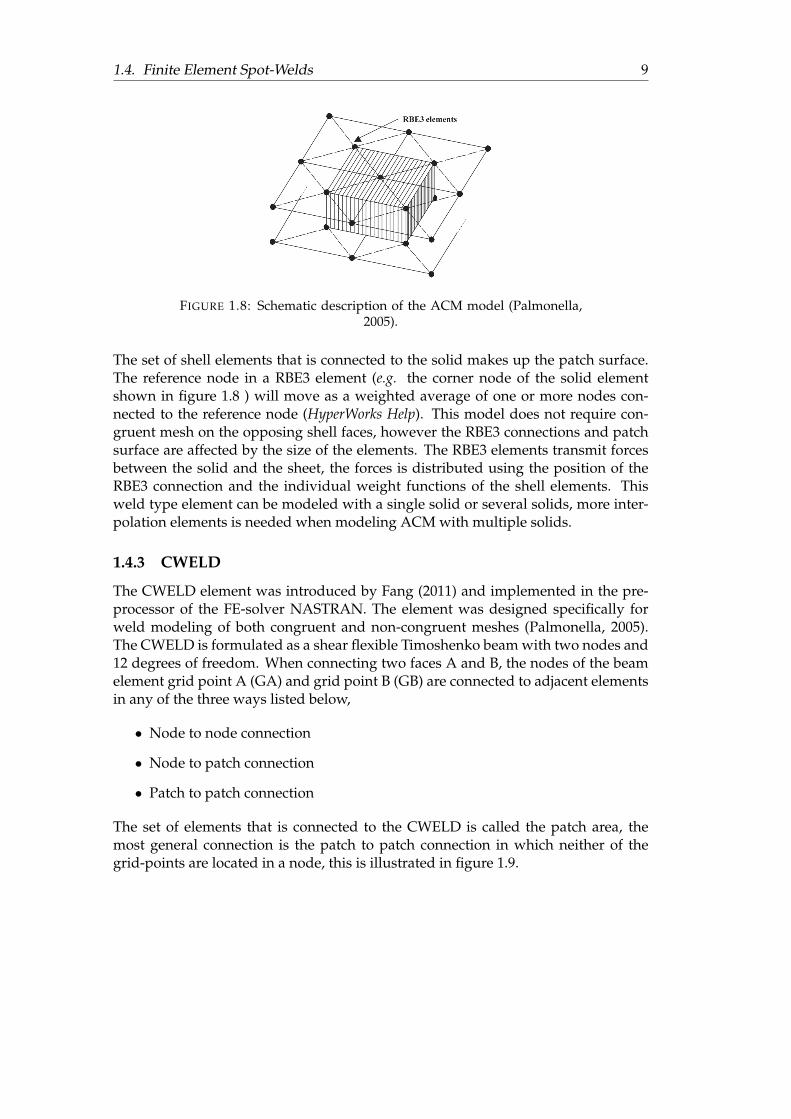
One of the most commonly used spot-weld models was proposed by Heiserer et.al(1999) and is called the area contact method or ACM. The weld is modeled with asolid hexahedral element which represents the weld nugget, in Hypermesh 2017.2this element is by default a first order element with 8 nodes called HEX8 (HyperWorksHelp). A special type of interpolation elements known as rigid bar element 3 (RBE3)is used to connect the nodes in this hexahedral element with adjacent nodes in thecorresponding shell elements. A schematic description of the ACM model is shownin figure 1.8.
1.4. Finite Element Spot-Welds 9
FIGURE 1.8: Schematic description of the ACM model (Palmonella,2005).
The set of shell elements that is connected to the solid makes up the patch surface.The reference node in a RBE3 element (e.g. the corner node of the solid elementshown in figure 1.8 ) will move as a weighted average of one or more nodes con-nected to the reference node (HyperWorks Help). This model does not require con-gruent mesh on the opposing shell faces, however the RBE3 connections and patchsurface are affected by the size of the elements. The RBE3 elements transmit forcesbetween the solid and the sheet, the forces is distributed using the position of theRBE3 connection and the individual weight functions of the shell elements. Thisweld type element can be modeled with a single solid or several solids, more inter-polation elements is needed when modeling ACM with multiple solids.
1.4.3 CWELD
The CWELD element was introduced by Fang (2011) and implemented in the pre-processor of the FE-solver NASTRAN. The element was designed specifically forweld modeling of both congruent and non-congruent meshes (Palmonella, 2005).The CWELD is formulated as a shear flexible Timoshenko beam with two nodes and12 degrees of freedom. When connecting two faces A and B, the nodes of the beamelement grid point A (GA) and grid point B (GB) are connected to adjacent elementsin any of the three ways listed below,
• Node to node connection
• Node to patch connection
• Patch to patch connection
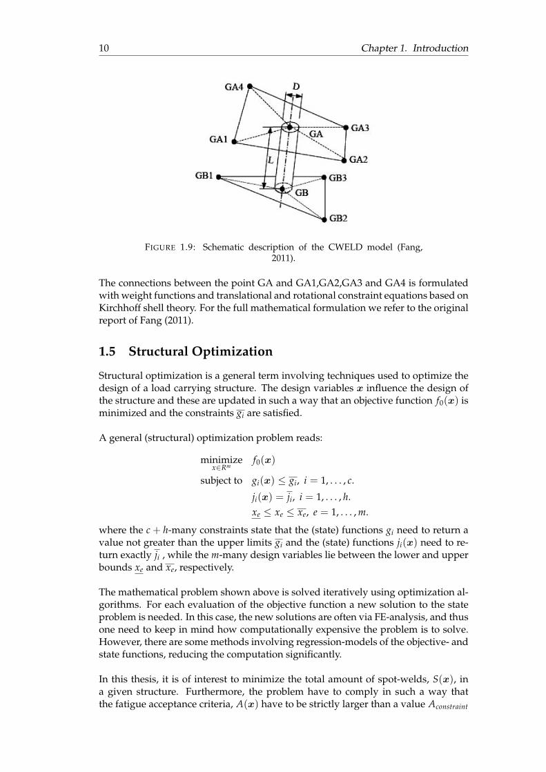
The set of elements that is connected to the CWELD is called the patch area, themost general connection is the patch to patch connection in which neither of thegrid-points are located in a node, this is illustrated in figure 1.9.
10 Chapter 1. Introduction
FIGURE 1.9: Schematic description of the CWELD model (Fang,2011).
The connections between the point GA and GA1,GA2,GA3 and GA4 is formulatedwith weight functions and translational and rotational constraint equations based onKirchhoff shell theory. For the full mathematical formulation we refer to the originalreport of Fang (2011).
1.5 Structural Optimization
Structural optimization is a general term involving techniques used to optimize thedesign of a load carrying structure. The design variables x influence the design ofthe structure and these are updated in such a way that an objective function f0(x) isminimized and the constraints gi are satisfied.
A general (structural) optimization problem reads:
minimizex∈Rm
f0(x)
subject to gi(x) ≤ gi, i = 1, . . . , c.
ji(x) = ji, i = 1, . . . , h.xe ≤ xe ≤ xe, e = 1, . . . , m.
where the c + h-many constraints state that the (state) functions gi need to return avalue not greater than the upper limits gi and the (state) functions ji(x) need to re-turn exactly ji , while the m-many design variables lie between the lower and upperbounds xe and xe, respectively.
The mathematical problem shown above is solved iteratively using optimization al-gorithms. For each evaluation of the objective function a new solution to the stateproblem is needed. In this case, the new solutions are often via FE-analysis, and thusone need to keep in mind how computationally expensive the problem is to solve.However, there are some methods involving regression-models of the objective- andstate functions, reducing the computation significantly.
In this thesis, it is of interest to minimize the total amount of spot-welds, S(x), ina given structure. Furthermore, the problem have to comply in such a way thatthe fatigue acceptance criteria, A(x) have to be strictly larger than a value Aconstraint
1.5. Structural Optimization 11
when returning the optimal amount of spot-welds.
The optimization problem of this thesis is formulated in a simple manner:
minimizex∈Rm
S(x)
subject to − A(x) ≤ −Aconstraint (∗)xe ≤ xe ≤ xe, e = 1, . . . , m.
* Minus signs were added for the sake of not switching the inequality sign.
The design variable x of the above formulation involves the spot-welds themselves,but are perceived somewhat differently depending of what kind of optimization ap-proach is used, this is thoroughly explained in section 1.5.2 and 1.5.3. The locationof the spot-weld is also of major importance to a constraint such as fatigue life, andwill be handled and described further in other sections. Additional constraints willalso be introduced later, e.g stiffness and eigenfrequency, for the sake of benchmark-ing different optimization methods compatibility and performance using multipleconstraints.
1.5.1 Pitfalls and Possibilities of Optimization Problems
During the design process of a product, characteristics such as efficiency, reliability,economy and structural capabilities are important to consider and makes the prod-uct more desirable to customers. Embodying all these parameters into one singleoptimization when designing is called multidisciplinary design optimization, MDO.The optimum from an MDO problem is a superior design compared to one that hasbeen iteratively found by optimizing each discipline sequentially. MDO has the ben-efit of exploiting the interactions between the disciplines. However, optimizing forseveral constraints simultaneously will significantly increase the complexity of theproblem definition.
ConvexityWhen an optimization problem increases in size it is crucial to identify whether itis convex or not. An identified optimum for a non-convex problem may be a localone, leaving the global optimum still undiscovered. Contrary, a convex optimizationproblem can only have one optimum which is consequently globally optimal.
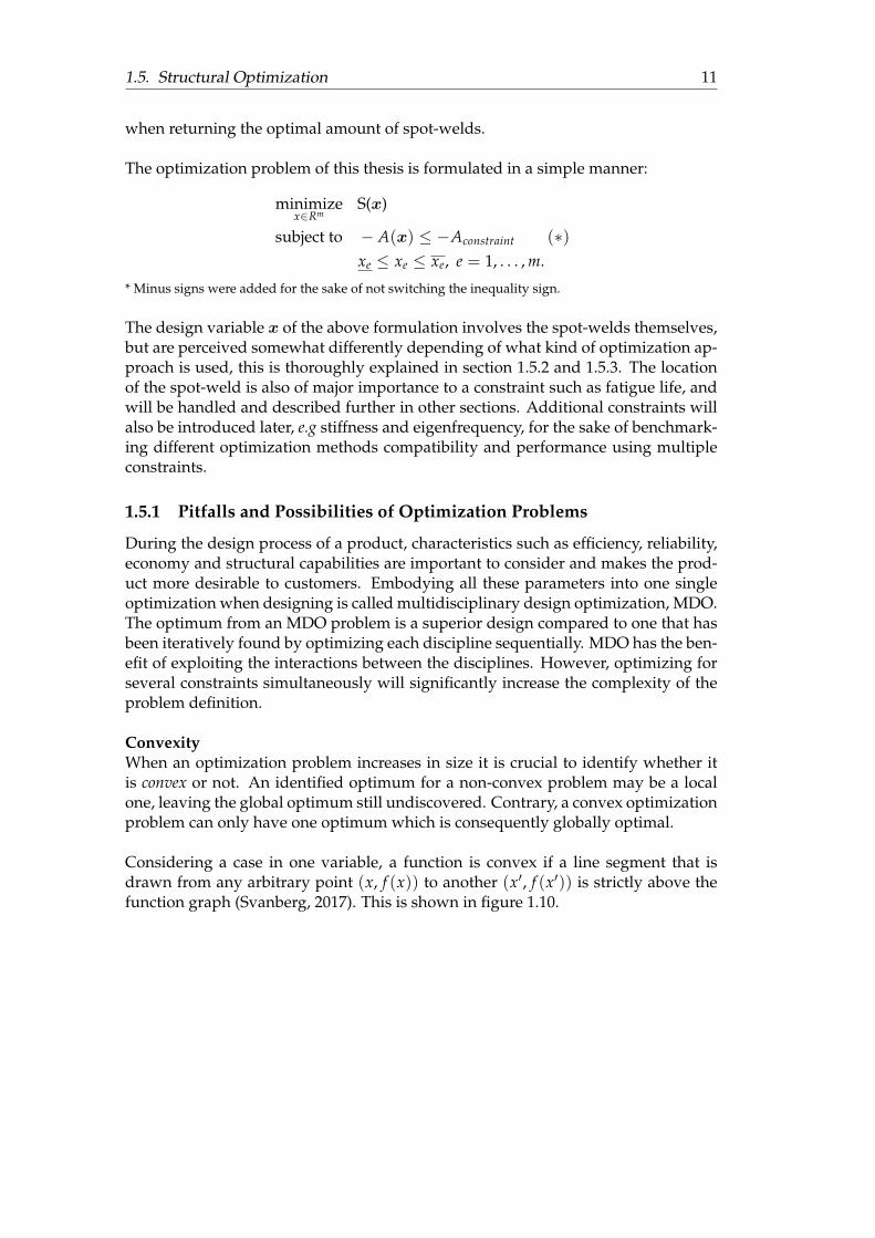
Considering a case in one variable, a function is convex if a line segment that isdrawn from any arbitrary point (x, f (x)) to another (x′, f (x′)) is strictly above thefunction graph (Svanberg, 2017). This is shown in figure 1.10.
12 Chapter 1. Introduction
FIGURE 1.10: Example of a convex and non-convex (objective) func-tion (Svanberg, 2017).
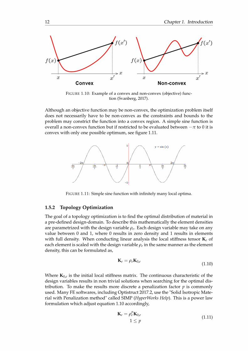
Although an objective function may be non-convex, the optimization problem itselfdoes not necessarily have to be non-convex as the constraints and bounds to theproblem may constrict the function into a convex region. A simple sine function isoverall a non-convex function but if restricted to be evaluated between −π to 0 it isconvex with only one possible optimum, see figure 1.11.
FIGURE 1.11: Simple sine function with infinitely many local optima.
1.5.2 Topology Optimization
The goal of a topology optimization is to find the optimal distribution of material ina pre-defined design-domain. To describe this mathematically the element densitiesare parametrized with the design variable ρe. Each design variable may take on anyvalue between 0 and 1, where 0 results in zero density and 1 results in elementswith full density. When conducting linear analysis the local stiffness tensor Ke ofeach element is scaled with the design variable ρe in the same manner as the elementdensity, this can be formulated as,
Ke = ρeK0,e (1.10)
Where K0,e is the initial local stiffness matrix. The continuous characteristic of thedesign variables results in non trivial solutions when searching for the optimal dis-tribution. To make the results more discrete a penalization factor p is commonlyused. Many FE softwares, including Optistruct 2017.2, use the "Solid Isotropic Mate-rial with Penalization method" called SIMP (HyperWorks Help). This is a power lawformulation which adjust equation 1.10 accordingly,
Ke = ρpe K0,e
1 ≤ p(1.11)
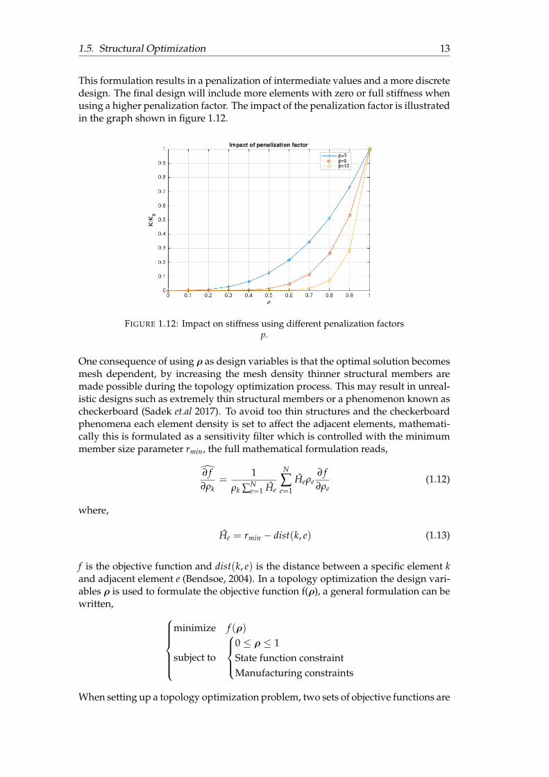
1.5. Structural Optimization 13
This formulation results in a penalization of intermediate values and a more discretedesign. The final design will include more elements with zero or full stiffness whenusing a higher penalization factor. The impact of the penalization factor is illustratedin the graph shown in figure 1.12.
FIGURE 1.12: Impact on stiffness using different penalization factorsp.
One consequence of using ρ as design variables is that the optimal solution becomesmesh dependent, by increasing the mesh density thinner structural members aremade possible during the topology optimization process. This may result in unreal-istic designs such as extremely thin structural members or a phenomenon known ascheckerboard (Sadek et.al 2017). To avoid too thin structures and the checkerboardphenomena each element density is set to affect the adjacent elements, mathemati-cally this is formulated as a sensitivity filter which is controlled with the minimummember size parameter rmin, the full mathematical formulation reads,
∂ f∂ρk
=1
ρk ∑Ne=1 He
N
∑e=1
Heρe∂ f∂ρe
(1.12)
where,
He = rmin − dist(k, e) (1.13)
f is the objective function and dist(k, e) is the distance between a specific element kand adjacent element e (Bendsoe, 2004). In a topology optimization the design vari-ables ρ is used to formulate the objective function f(ρ), a general formulation can bewritten,
minimize f (ρ)
subject to
0 ≤ ρ ≤ 1State function constraintManufacturing constraints
When setting up a topology optimization problem, two sets of objective functions are
14 Chapter 1. Introduction
commonly used, namely minimize volume or minimize structural flexibility. Usingthe volume the objective function reads,
minimize V =N
∑e=1
ρpe V0,e (1.14)
Where e denotes the individual element number and V0,e is the initial element vol-ume. Using the flexibility, (also known as compliance) the objective function reads,
minimize C =N
∑e=1
ρpe uT
e K0,eue (1.15)
Where ue is the local displacement vector and K0,e is the initial local stiffness matrix.
Method of Feasible DirectionsThe topology optimization setup results in a non-linear optimization problem. Tosolve such a problem, a non-linear solver algorithm is used. HyperMesh 2017.2uses a gradient based solver algorithm called method of feasible directions, MFD,considering the non-linear optimization problem,
minimizex∈Rm
f (xi)
subject to gj(xi) ≤ 0 ∀j(1.16)
where i denotes the iteration number. The method of feasible direction is based ona initial starting point xi that is within the feasible space. This point is iterativelyupdated in the following manner,
xi+1 = xi + λidi (1.17)
Where λi is the step size and di is the directional vector. By moving in a directionsuch that the objective function decreases and the constraints is met, the optimumis reached (Zoutendijk, 1959). To find such a direction among the infinite number ofdirections a set of conditions is used,
di∇ f (xi) < 0
di∇gj(xi) ≤ 0 ∀j(1.18)
where the first condition renders the descent direction and the second conditionrenders the feasible direction. These conditions are closely related to the conditionsknown as the Karush-Kuhn-Tucker or KKT-conditions (Zoutendijk, 1959). ∇ f (xi)and ∇gj(xi) are the gradients of the objective function and constraints respectively.Directional vectors di that satisfies both conditions is sought, these are called us-able directions. One way to find a usable direction is to solve the following linearoptimization,
minimizex∈Rm
− β
subject to β = - max{dTi ∇ f (xi) , dT
i ∇gj(xi)} ∀j
dTi ∇ f (xi) + β ≤ 0
dTi ∇gj(xi) + β ≤ 0 ∀j
0 < β
dTi d = 1
(1.19)
1.5. Structural Optimization 15
If βopt < ε1 then a optimal solution has been found (xi = xopt) and the solver stops,ε1 is a pre-defined small number. If βopt ≥ ε1 then di,opt is combined with equation1.17 , the step size is determined by,
λi :
{∂ f (λi)
∂λi= 0
gj(λi) ≤ 0(1.20)
The solver stops at this stage (xi = xopt) if the following conditions is met,∣∣∣∣ f (xi)− f (xi+1)
f (xi)
∣∣∣∣ < ε2
||xi − xi+1|| < ε3
(1.21)
Where ε2 and ε3 are small numbers. If the conditions in equation 1.21 is not met xi+1is put back into equation 1.19 for a new iteration.
1.5.3 Size Optimization with Response Surfaces and Genetic Algorithms
Size optimization is a broad term that involves parameterizing anything that is ofinterest to be changed on a structure into a design variable, e.g thickness, with aminimum expense of certain factors such as weight and economy. Unlike topologyoptimization, the design variables are not penalized and forced to an upper or lowerlimit.
Most size optimization problems require experiments and/or simulations to evalu-ate objective and constraints as functions of the desired design variables. However,a single experiment or simulation can take hours or even days to complete. As aresult, design optimization become unreasonable since they may require thousandsor even millions of simulation evaluations.
Response Surfaces and Design of ExperimentsIn consideration of the aforementioned problem, generating models called responsesurfaces (also referred to as metamodels or surrogate models) would be more feasible.Response surfaces mimic the behavior of the simulation model as closely as possi-ble while using as few as possible evaluation points for regression. When only onesingle design variable is involved, the process is simply known as curve fitting.
A general (linear) regression model is of the form
y(x) = c1ψ1(x) + c2ψ2(x) + . . . + cnψn(x) (1.22)
and can be used to create response surfaces. ψ are the arbitrary linearly independentbasis functions and ci are the coefficients that has to be determined by a least squarefit by minimizing the sum of the square of the errors y(xi) − gi, where gi are thesample data shown in equation 1.23.
c1ψ1(x1) + c2ψ2(x1) + . . . + cnψn(x1) = g1
c1ψ1(x2) + c2ψ2(x2) + . . . + cnψn(x2) = g2...c1ψ1(xm) + c2ψ2(xm) + . . . + cnψn(xm) = gm
(1.23)
16 Chapter 1. Introduction
The regression model for a second-order response surface can be formulated as,
y = β0 +k
∑j=1
β jxj + ∑ ∑i<j
βijxixj +k
∑j=1
β jjx2j (1.24)
This is equivalent to a first-order regression model, with exception for β jjx2j which is
the quadratic terms and βijxixj which are the interactions.
Referring back to equations 1.22 and 1.23, instead of using simple polynomials suchas in the equation above, the functions ψi can be described as radial basis functions,
ψi(x) = ψi(‖x− xi‖) = ψi(r) (1.25)
where r is the distance between the points x and xi, hence why this model is calledthe radial basis model (RBF). The functions ψi(e) have many forms and are alwaysradially symmetric. The most common is the Gaussian function:
ψ(r) = e−(rk )
2(1.26)
where k is a shape parameter.
An additional response surface model is the Kriging model, this model has the bene-fit of interpolating between data points. Kriging is a combination of the polynomialregression model and a random function Z(x). In a polynomial regression model,the coefficients are chosen so that the error between the given data and model areminimized. However the random function Z(x) reduces this error to zero so that themodel interpolates the given data points.
The accuracy of the response surface depends on the number and locations of thedata points that have been evaluated in the design space. It is important that thedata points are chosen so that the response surface has a proper input-output behav-ior. There are various so called design of experiments (DOE) that cater to differentsources of errors, in particular errors due to noise in the data or due to an improperresponse surface. The following are three common design of experiments:
• Randomized sampling, often known as Monte Carlo simulations, samples fromstochastic variables based upon a chosen probability density function. Themost common probability density function used is the Gaussian function. Al-though simple to apply, the drawback is that many simulations are needed toget good accuracy.
• The Latin Hypercube method inherits the stochastic properties of the MonteCarlo method, but work in a different manner as the points chosen are morecomputationally efficient. A square grid containing sample positions is a Latinsquare if, and only if, there is only one sample in each row and each column.A Latin Hypercube DOE, categorized as a space filling DOE, is the generaliza-tion of this concept to an arbitrary number of dimensions. The application isrelatively more difficult than the normal Monte Carlo method since the DOEhas to remember all the previous sample points when creating a new one. Seefigure 1.13.
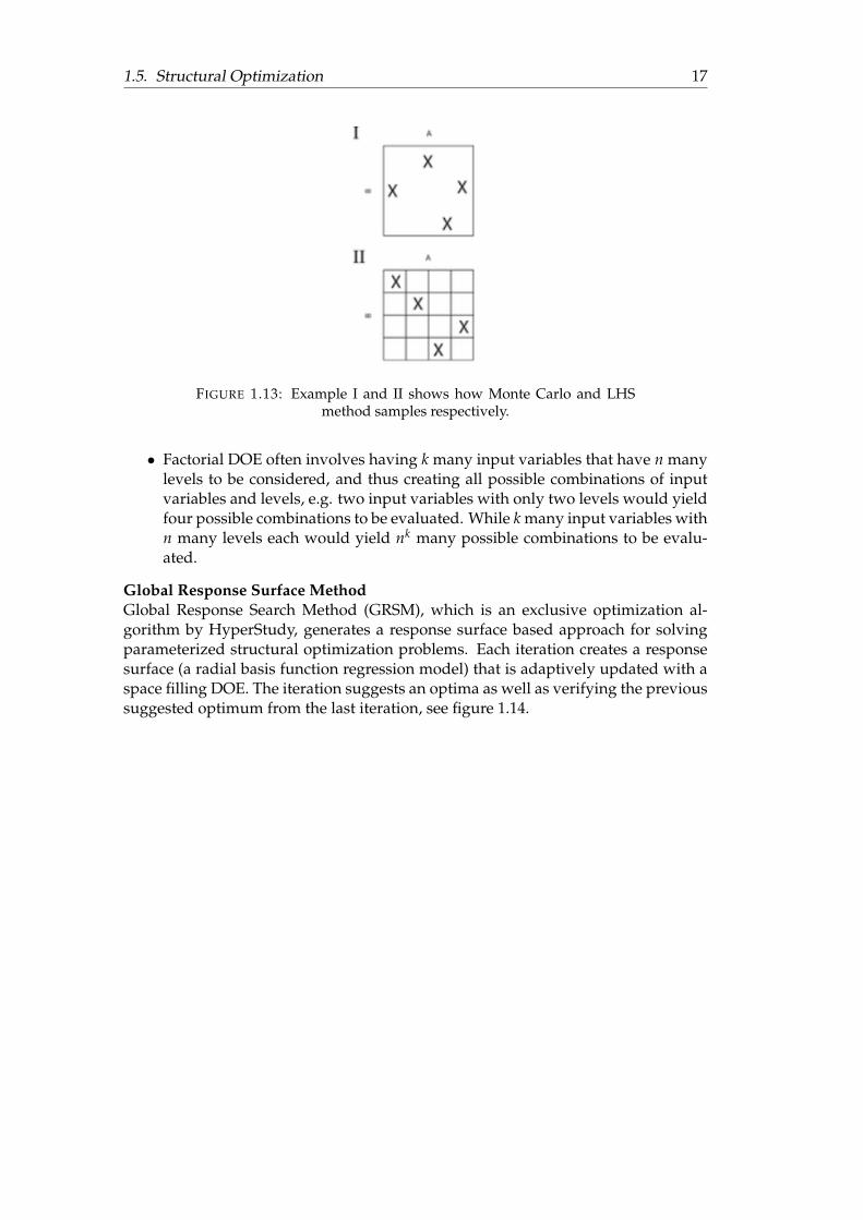
1.5. Structural Optimization 17
FIGURE 1.13: Example I and II shows how Monte Carlo and LHSmethod samples respectively.
• Factorial DOE often involves having k many input variables that have n manylevels to be considered, and thus creating all possible combinations of inputvariables and levels, e.g. two input variables with only two levels would yieldfour possible combinations to be evaluated. While k many input variables withn many levels each would yield nk many possible combinations to be evalu-ated.
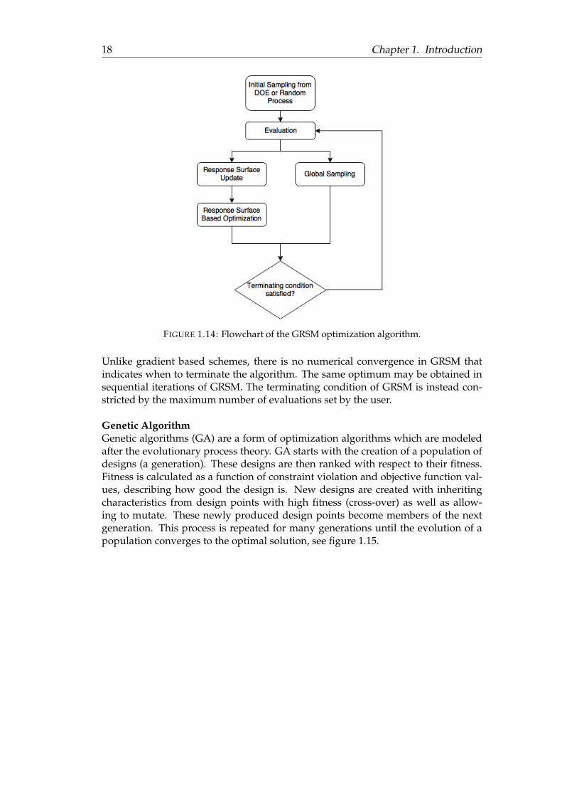
Global Response Surface MethodGlobal Response Search Method (GRSM), which is an exclusive optimization al-gorithm by HyperStudy, generates a response surface based approach for solvingparameterized structural optimization problems. Each iteration creates a responsesurface (a radial basis function regression model) that is adaptively updated with aspace filling DOE. The iteration suggests an optima as well as verifying the previoussuggested optimum from the last iteration, see figure 1.14.
18 Chapter 1. Introduction
FIGURE 1.14: Flowchart of the GRSM optimization algorithm.
Unlike gradient based schemes, there is no numerical convergence in GRSM thatindicates when to terminate the algorithm. The same optimum may be obtained insequential iterations of GRSM. The terminating condition of GRSM is instead con-stricted by the maximum number of evaluations set by the user.
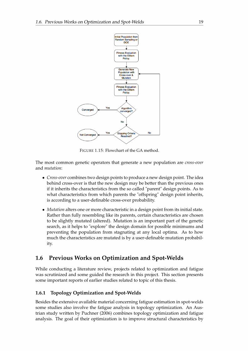
Genetic AlgorithmGenetic algorithms (GA) are a form of optimization algorithms which are modeledafter the evolutionary process theory. GA starts with the creation of a population ofdesigns (a generation). These designs are then ranked with respect to their fitness.Fitness is calculated as a function of constraint violation and objective function val-ues, describing how good the design is. New designs are created with inheritingcharacteristics from design points with high fitness (cross-over) as well as allow-ing to mutate. These newly produced design points become members of the nextgeneration. This process is repeated for many generations until the evolution of apopulation converges to the optimal solution, see figure 1.15.
1.6. Previous Works on Optimization and Spot-Welds 19
FIGURE 1.15: Flowchart of the GA method.
The most common genetic operators that generate a new population are cross-overand mutation:
• Cross-over combines two design points to produce a new design point. The ideabehind cross-over is that the new design may be better than the previous onesif it inherits the characteristics from the so called "parent" design points. As towhat characteristics from which parents the "offspring" design point inherits,is according to a user-definable cross-over probability.
• Mutation alters one or more characteristic in a design point from its initial state.Rather than fully resembling like its parents, certain characteristics are chosento be slightly mutated (altered). Mutation is an important part of the geneticsearch, as it helps to "explore" the design domain for possible minimums andpreventing the population from stagnating at any local optima. As to howmuch the characteristics are mutated is by a user-definable mutation probabil-ity.
1.6 Previous Works on Optimization and Spot-Welds
While conducting a literature review, projects related to optimization and fatiguewas scrutinized and some guided the research in this project. This section presentssome important reports of earlier studies related to topic of this thesis.
1.6.1 Topology Optimization and Spot-Welds
Besides the extensive available material concerning fatigue estimation in spot-weldssome studies also involve the fatigue analysis in topology optimization. An Aus-trian study written by Puchner (2006) combines topology optimization and fatigueanalysis. The goal of their optimization is to improve structural characteristics by
20 Chapter 1. Introduction
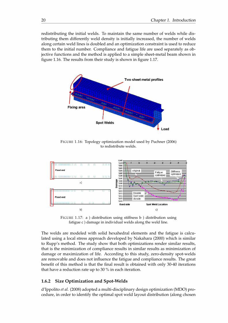
redistributing the initial welds. To maintain the same number of welds while dis-tributing them differently weld density is initially increased, the number of weldsalong certain weld lines is doubled and an optimization constraint is used to reducethem to the initial number. Compliance and fatigue life are used separately as ob-jective functions and the method is applied to a simple sheet-metal beam shown infigure 1.16. The results from their study is shown in figure 1.17.
FIGURE 1.16: Topology optimization model used by Puchner (2006)to redistribute welds.
FIGURE 1.17: a ) distribution using stiffness b ) distribution usingfatigue c ) damage in individual welds along the weld line.
The welds are modeled with solid hexahedral elements and the fatigue is calcu-lated using a local stress approach developed by Nakahara (2000) which is similarto Rupp’s method. The study show that both optimizations render similar results,that is the minimization of compliance results in similar results as minimization ofdamage or maximization of life. According to this study, zero-density spot-weldsare removable and does not influence the fatigue and compliance results. The greatbenefit of this method is that the final result is obtained with only 30-40 iterationsthat have a reduction rate up to 30 % in each iteration.
1.6.2 Size Optimization and Spot-Welds
d’Ippolito et al. (2008) adopted a multi-disciplinary design optimization (MDO) pro-cedure, in order to identify the optimal spot weld layout distribution (along chosen
1.6. Previous Works on Optimization and Spot-Welds 21
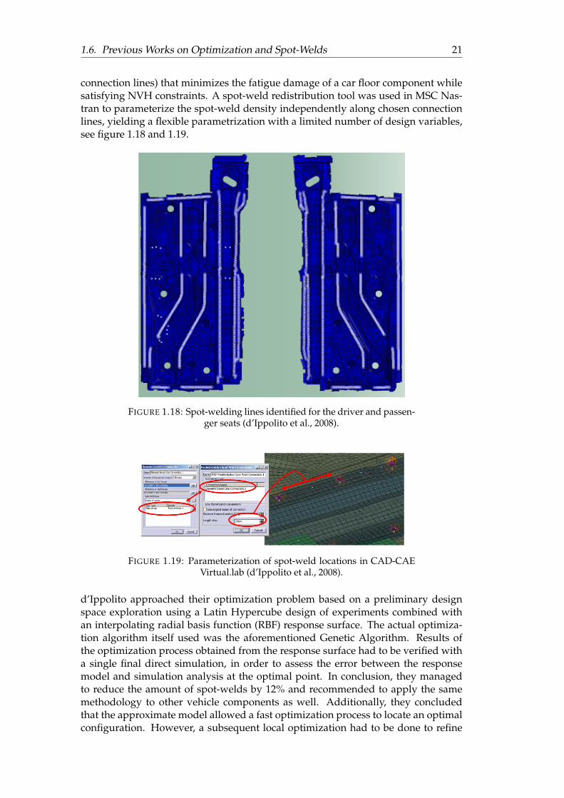
connection lines) that minimizes the fatigue damage of a car floor component whilesatisfying NVH constraints. A spot-weld redistribution tool was used in MSC Nas-tran to parameterize the spot-weld density independently along chosen connectionlines, yielding a flexible parametrization with a limited number of design variables,see figure 1.18 and 1.19.
FIGURE 1.18: Spot-welding lines identified for the driver and passen-ger seats (d’Ippolito et al., 2008).
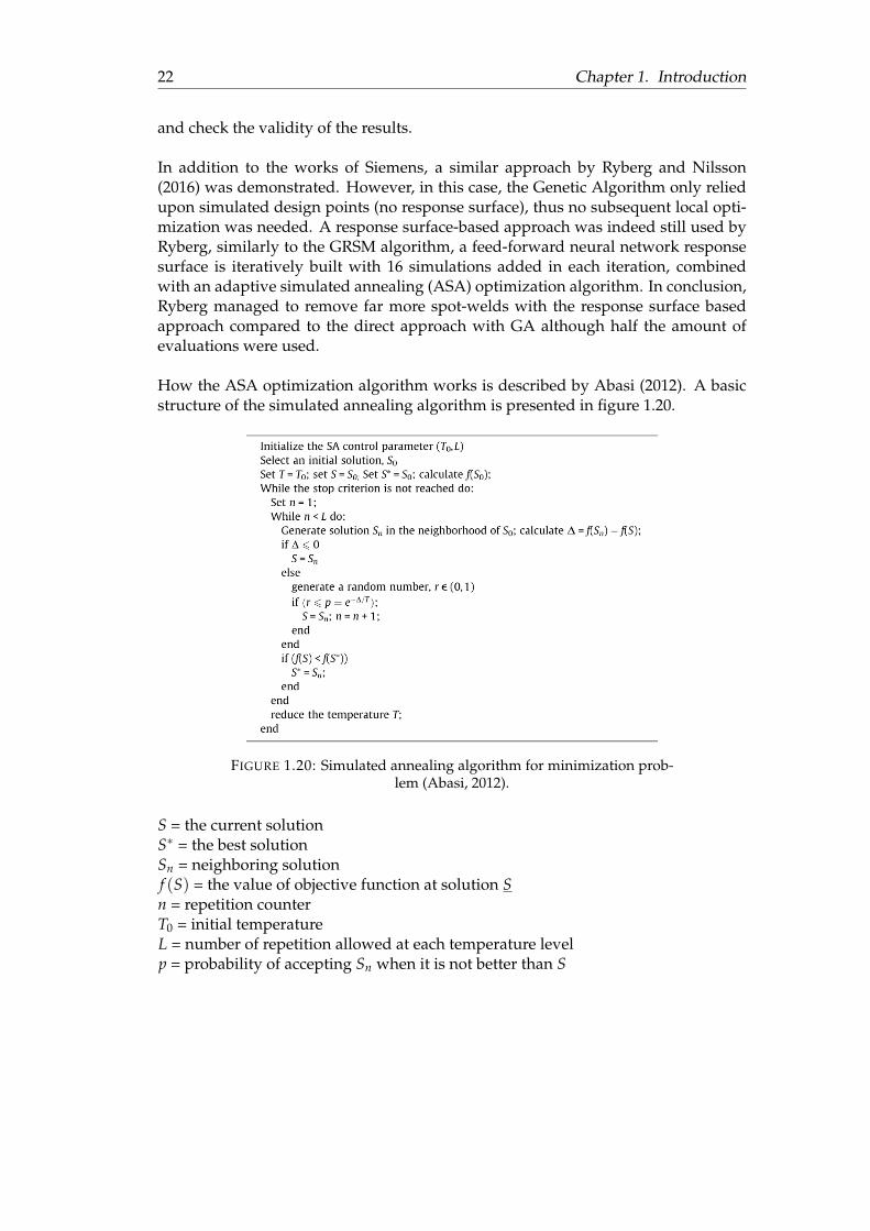
FIGURE 1.19: Parameterization of spot-weld locations in CAD-CAEVirtual.lab (d’Ippolito et al., 2008).
d’Ippolito approached their optimization problem based on a preliminary designspace exploration using a Latin Hypercube design of experiments combined withan interpolating radial basis function (RBF) response surface. The actual optimiza-tion algorithm itself used was the aforementioned Genetic Algorithm. Results ofthe optimization process obtained from the response surface had to be verified witha single final direct simulation, in order to assess the error between the responsemodel and simulation analysis at the optimal point. In conclusion, they managedto reduce the amount of spot-welds by 12% and recommended to apply the samemethodology to other vehicle components as well. Additionally, they concludedthat the approximate model allowed a fast optimization process to locate an optimalconfiguration. However, a subsequent local optimization had to be done to refine
22 Chapter 1. Introduction
and check the validity of the results.
In addition to the works of Siemens, a similar approach by Ryberg and Nilsson(2016) was demonstrated. However, in this case, the Genetic Algorithm only reliedupon simulated design points (no response surface), thus no subsequent local opti-mization was needed. A response surface-based approach was indeed still used byRyberg, similarly to the GRSM algorithm, a feed-forward neural network responsesurface is iteratively built with 16 simulations added in each iteration, combinedwith an adaptive simulated annealing (ASA) optimization algorithm. In conclusion,Ryberg managed to remove far more spot-welds with the response surface basedapproach compared to the direct approach with GA although half the amount ofevaluations were used.
How the ASA optimization algorithm works is described by Abasi (2012). A basicstructure of the simulated annealing algorithm is presented in figure 1.20.
FIGURE 1.20: Simulated annealing algorithm for minimization prob-lem (Abasi, 2012).
S = the current solutionS∗ = the best solutionSn = neighboring solutionf (S) = the value of objective function at solution Sn = repetition counterT0 = initial temperatureL = number of repetition allowed at each temperature levelp = probability of accepting Sn when it is not better than S
23
Chapter 2
Method
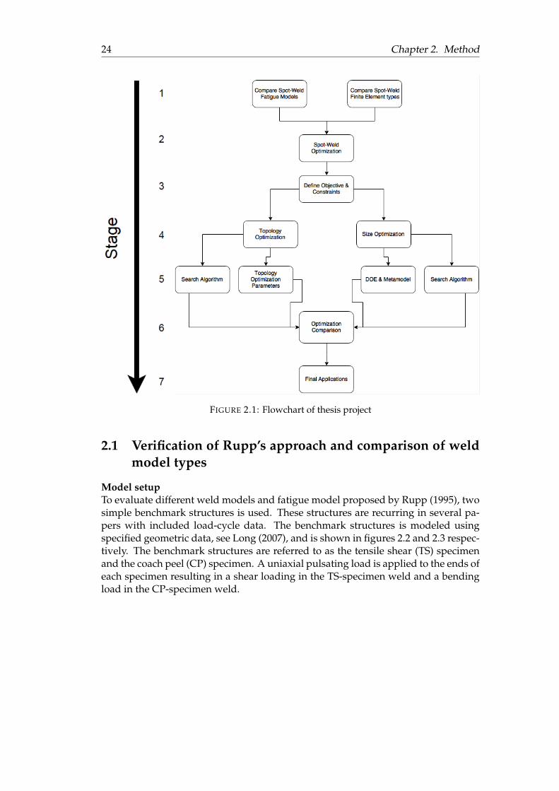
In this thesis project, the research is conducted in accordance with the work-flowshown in figure 2.1. The study starts with an investigation of current weld meth-ods. By reviewing the literature and by consultation with FE software developers,different approaches are identified. Ways of evaluating fatigue in and around thecandidate welds are then considered. By exploring current methods and their ap-plicability and compatibility to spot-welded joints, a number of viable methods areidentified. The candidate weld models and fatigue calculation methods are thenevaluated using single-weld benchmark structures, for more details, see section 2.1.These steps mark the first stage in the work-flow described in figure 2.1.
By evaluating the results from the first stage the weld model and fatigue calculationthat renders best results is then considered for optimization. The second stage of thisstudy is dedicated to investigating different optimization approaches. Strengths andlimitations are identified by a literature review and, at this stage, the compatibilitywith weld optimization is considered. The single weld benchmark structures is thenreplaced by a multi-weld model which can be used to implement two different op-timization approaches, topology and size optimization. This concludes the secondstage of the work-flow shown in figure 2.1.
The multi-weld model originates from a paper written by Ryberg and Nilsson (2016),stage three to five involves the model and optimization problem setup for topologyand size optimization, this is described in greater detail in section 2.3 and 2.4 re-spectively. As indicated in figure 2.1, the results from the two approaches are thencompared in stage six and more about the comparison is found in section 2.5. In afinal stage the topology optimization with fatigue constraints is applied to a full sizecar model supplied by Combitech, to evaluate the method on a large-scale applica-tion. The size optimization is combined with a non-linear load-case to evaluate itsability to handle more complex analysis. The last stage of the work-flow is describedin section 2.6.
24 Chapter 2. Method
FIGURE 2.1: Flowchart of thesis project
2.1 Verification of Rupp’s approach and comparison of weldmodel types
Model setupTo evaluate different weld models and fatigue model proposed by Rupp (1995), twosimple benchmark structures is used. These structures are recurring in several pa-pers with included load-cycle data. The benchmark structures is modeled usingspecified geometric data, see Long (2007), and is shown in figures 2.2 and 2.3 respec-tively. The benchmark structures are referred to as the tensile shear (TS) specimenand the coach peel (CP) specimen. A uniaxial pulsating load is applied to the ends ofeach specimen resulting in a shear loading in the TS-specimen weld and a bendingload in the CP-specimen weld.

2.1. Verification of Rupp’s approach and comparison of weld model types 25
FIGURE 2.2: Schematic description of single weld tensile shear (TS)specimen, dimensions in mm
FIGURE 2.3: Schematic description of single weld coach peel (CP)specimen, dimensions in mm
The sheet metal in each specimen is modeled with first order quadrilateral shell ele-ments called QUAD4. The single weld is modeled with the weld element candidatesdescribed in the previous chapter. The models are prepared in the pre-processor Hy-permesh 2017.2. The meshed TS and CP specimens are shown in figures 2.4 and 2.5respectively. An element size of 1mm is initially used. The spot-weld diameter isset to match the physical diameter of the weld, the material of the sheet metal aredefined in the fatigue module and is presented in table 2.1.
26 Chapter 2. Method
FIGURE 2.4: Uniaxially loaded tensile shear (TS) specimen, meshedwith element size 1mm.
FIGURE 2.5: Uniaxially loaded coach peel (CP) specimen, meshedwith element size 1mm.
Fatigue setupThe fatigue evaluation can be summarized as a separate workflow shown in figure2.6. Fy shown in figures 2.4 and 2.5 is applied as line loads, which are used to solvethe linear static sub-cases. These loads are then scaled in the fatigue tool to matchthe experimental fatigue loads. In the fatigue sub-case, these loads are applied in asinusoidal cycle using the load ratio R = 0.1 which is defined as
R =σmin
σmax=
Fmin
Fmax(2.1)
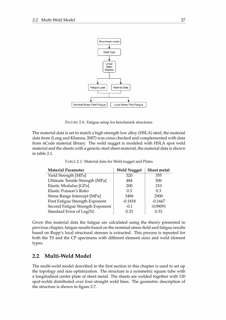
2.2. Multi-Weld Model 27
FIGURE 2.6: Fatigue setup for benchmark structures
The material data is set to match a high strength low alloy (HSLA) steel, the materialdata from (Long and Khanna, 2007) was cross-checked and complemented with datafrom nCode material library. The weld nugget is modeled with HSLA spot weldmaterial and the sheets with a generic steel sheet material, the material data is shownin table 2.1.
TABLE 2.1: Material data for Weld nugget and Plates
Material Parameter Weld Nugget Sheet metalYield Strength [MPa] 320 355Ultimate Tensile Strength [MPa] 484 500Elastic Modulus [GPa] 200 210Elastic Poisson’s Ratio 0.3 0.3Stress Range Intercept [MPa] 3496 2900First Fatigue Strength Exponent -0.1818 -0.1667Second Fatigue Strength Exponent -0.1 -0.09091Standard Error of Log(N) 0.33 0.33
Given this material data the fatigue are calculated using the theory presented inprevious chapter, fatigue results based on the nominal stress-field and fatigue resultsbased on Rupp’s local structural stresses is extracted. This process is repeated forboth the TS and the CP specimens with different element sizes and weld elementtypes.
2.2 Multi-Weld Model
The multi-weld model described in the first section in this chapter is used to set upthe topology and size optimization. The structure is a symmetric square tube witha longitudinal center plate of sheet metal. The sheets are welded together with 120spot-welds distributed over four straight weld lines. The geometric description ofthe structure is shown in figure 2.7.
28 Chapter 2. Method
FIGURE 2.7: Geometric description of multi-weld model.
Note that the center plate is connected through 3-layer spot-welds, that is threesheets and two weld elements shown in 2.7 (B). Starting from either side of the struc-ture, the first, fifth and sixth weld in each weld line is considered a fixed weld. Thesheets are modeled with first order shell elements called QUAD4 and have a thick-ness of 1mm. The welds are modeled with any of the candidate spot-weld elementsand the weld diameter is set to 5mm. The structure is meshed in HyperMesh 2017.2and the element size is set to 5mm. Two static load-cases are considered. Forces andconstraints together with meshed structure are shown in figure 2.8 and 2.9, respec-tively.
FIGURE 2.8: Bending load-case, forces and constraints (Forces inNewtons).
2.3. Topology Optimization Setup 29
FIGURE 2.9: Torsion load-case, forces and constraints (Forces in New-tons).
For both optimization methods, a fatigue constraint on each individual spot-weld isimplemented. The fatigue is calculated via Rupp’s local structural stresses approach.Both static load cases are superposed and applied as a sinusoidal cycle with theload ratio R = −1. In addition to optimizing with respect to spot-weld fatigue, themulti-weld model will also be optimized with respect to several stiffness constraintsand an modal analysis constraint. One torsional stiffness constraint, Ct [N/deg], isintroduced via the torsional load case shown in figure 2.9, two stiffness constraints,Cbr (rocking motion) [N/mm] and Cbt (tunnel motion) [N/mm] are introduced viathe bending load case shown in figure 2.8. The modal analysis constraint is thesecond eigenfrequency which coincides with the first torsional mode. All constraintsare defined as 90% of the nominal run of the multi-weld model. This setup was usedfor both optimization methods described in section 2.3 and 2.4.
2.3 Topology Optimization Setup
The topology optimization is set up in the software Optistruct (OS), the design do-main is limited to the set of non-fixed weld elements. Nominally, there are 84 weldelements which may be removed. However these are distributed on 56 weld pointsince some welds are 3 layer welds (see previous section). The density and stiffnessof the elements are scaled by the design variables ρe, resulting in 84 design variablesin OS. One fatigue load-case is considered and the spot-weld fatigue is computedusing Rupp’s local structural stress approach. The static load-cases are applied asa sinusoidal cycle with the load ratio R = −1. Since only one fatigue load-case isconsidered, the local stresses are computed using superpositioning of stress from thebending and the torsion. Material parameters for welds and sheets are the same asfor the single weld simulations, which were shown in table 2.1. The optimizationproblem is solved using two different setups in OS,
• Minimization of volume fraction
• Minimization of weighted compliance.
30 Chapter 2. Method
By scaling the formulation given in equation 1.14 with the initial volumes, the firstsetup reads,
minimizeρ∈Rm
Vf (ρ)
subject to Vf (ρ) =∑N
e=1 ρpe V0e
V0, e
K(ρ) =N
∑e=1ρ
pe K0,e
K(ρ)U = FAconstraint ≤ A0 ≤ ρ ≤ 1
(2.2)
where Aconstraint is a pre-defined life or damage acceptance criteria. The second setupuses the formulation that is stated in equation 1.15 with the extra condition that sev-eral load-cases are considered. This is called a multi-objective optimization problemand uses weighted compliance. The formulation with constraints reads
minimizeρ∈Rm
C(C1(ρ), C2(ρ))
subject to C(ρ) =2
∑j=1
wjCj(ρ)
2
∑j=1
wj = 1
Cj(ρ) =N
∑e=1
ρpe uT
ejK0,euej
Kj(ρ)Uj = Fj
Aconstraint ≤ AVf (ρ) ≤ Vfconstraint
0 ≤ ρ ≤ 1
(2.3)
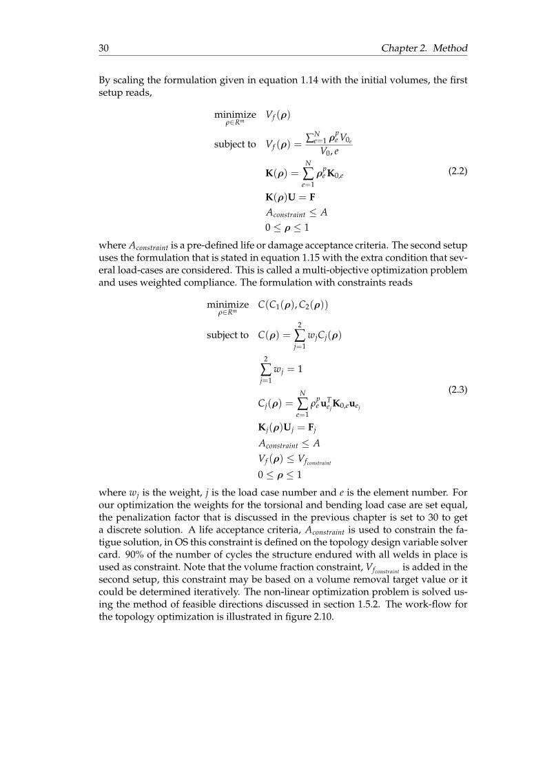
where wj is the weight, j is the load case number and e is the element number. Forour optimization the weights for the torsional and bending load case are set equal,the penalization factor that is discussed in the previous chapter is set to 30 to geta discrete solution. A life acceptance criteria, Aconstraint is used to constrain the fa-tigue solution, in OS this constraint is defined on the topology design variable solvercard. 90% of the number of cycles the structure endured with all welds in place isused as constraint. Note that the volume fraction constraint, Vfconstraint is added in thesecond setup, this constraint may be based on a volume removal target value or itcould be determined iteratively. The non-linear optimization problem is solved us-ing the method of feasible directions discussed in section 1.5.2. The work-flow forthe topology optimization is illustrated in figure 2.10.
2.4. Size Optimization Setup 31
FIGURE 2.10: Topology Optimization work-flow.
The optimization is also conducted using multiple linear constraints, this is done inorder to evaluate how well the optimization works when fatigue life is mixed withother constraints.
2.4 Size Optimization Setup
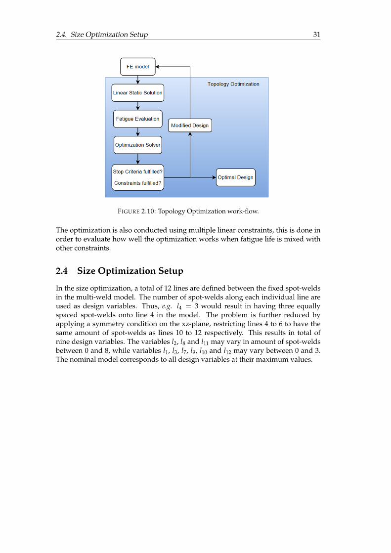
In the size optimization, a total of 12 lines are defined between the fixed spot-weldsin the multi-weld model. The number of spot-welds along each individual line areused as design variables. Thus, e.g. l4 = 3 would result in having three equallyspaced spot-welds onto line 4 in the model. The problem is further reduced byapplying a symmetry condition on the xz-plane, restricting lines 4 to 6 to have thesame amount of spot-welds as lines 10 to 12 respectively. This results in total ofnine design variables. The variables l2, l8 and l11 may vary in amount of spot-weldsbetween 0 and 8, while variables l1, l3, l7, l9, l10 and l12 may vary between 0 and 3.The nominal model corresponds to all design variables at their maximum values.
32 Chapter 2. Method
FIGURE 2.11: The Multi-Weld model with 12 spot-weld lines.
The above formulation is summarized in to an optimization problem shown below,
minimize f0 =12
∑i=1
li
subject to gi(x) ≤ gi, i = 1, . . . , c.l4 = l10
l5 = l11
l6 = l12
l1,3,7,9,10,12 ∈ {0, 1, 2, 3}l2,8,11 ∈ {0, 1, 2, . . . , 8}
The state functions gi(x) are in this case the torsional stiffness Ct, the bending stiff-nesses Cbr and Cbt, the first torsional eigenfrequency Fm2. The constraints gi are 90%of the nominal values of the state functions.
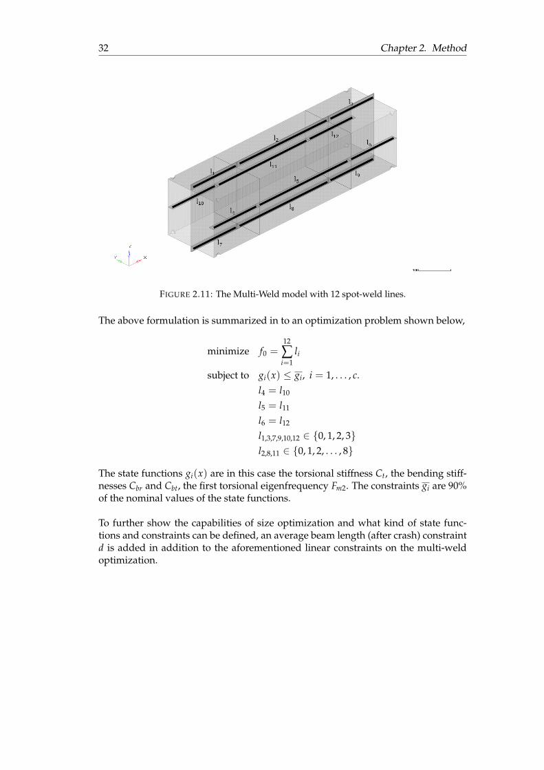
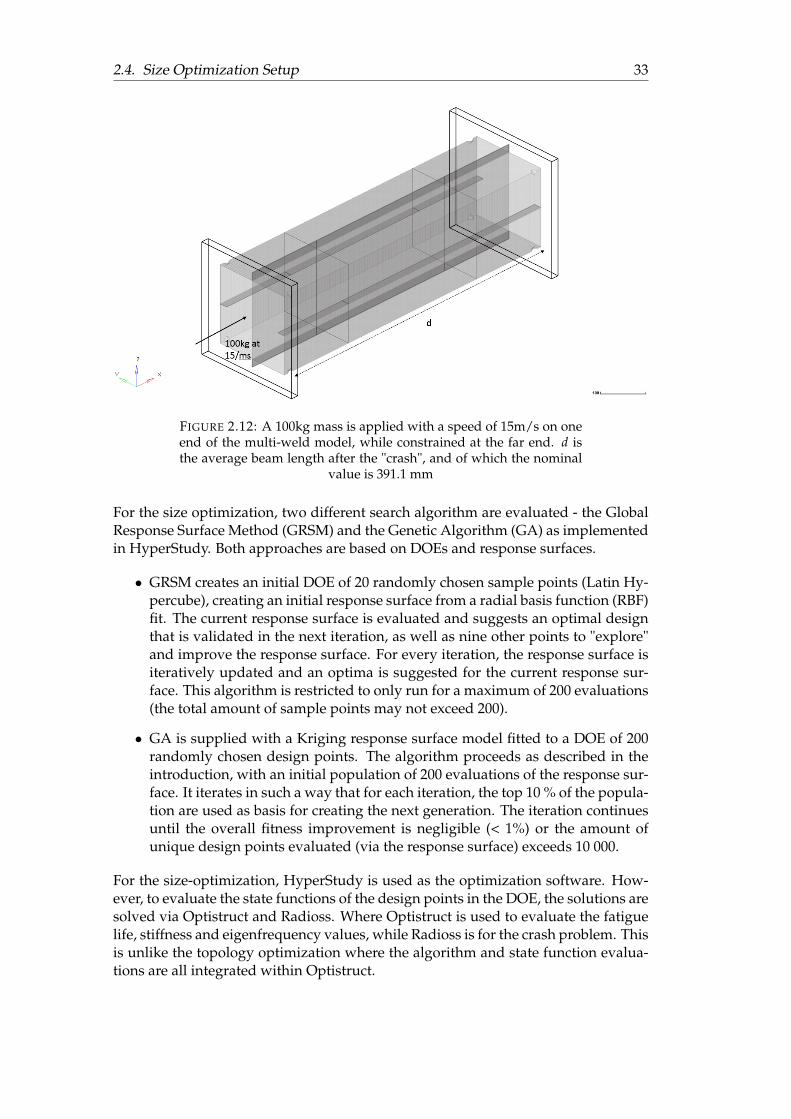
To further show the capabilities of size optimization and what kind of state func-tions and constraints can be defined, an average beam length (after crash) constraintd is added in addition to the aforementioned linear constraints on the multi-weldoptimization.
2.4. Size Optimization Setup 33
FIGURE 2.12: A 100kg mass is applied with a speed of 15m/s on oneend of the multi-weld model, while constrained at the far end. d isthe average beam length after the "crash", and of which the nominal
value is 391.1 mm
For the size optimization, two different search algorithm are evaluated - the GlobalResponse Surface Method (GRSM) and the Genetic Algorithm (GA) as implementedin HyperStudy. Both approaches are based on DOEs and response surfaces.
• GRSM creates an initial DOE of 20 randomly chosen sample points (Latin Hy-percube), creating an initial response surface from a radial basis function (RBF)fit. The current response surface is evaluated and suggests an optimal designthat is validated in the next iteration, as well as nine other points to "explore"and improve the response surface. For every iteration, the response surface isiteratively updated and an optima is suggested for the current response sur-face. This algorithm is restricted to only run for a maximum of 200 evaluations(the total amount of sample points may not exceed 200).
• GA is supplied with a Kriging response surface model fitted to a DOE of 200randomly chosen design points. The algorithm proceeds as described in theintroduction, with an initial population of 200 evaluations of the response sur-face. It iterates in such a way that for each iteration, the top 10 % of the popula-tion are used as basis for creating the next generation. The iteration continuesuntil the overall fitness improvement is negligible (< 1%) or the amount ofunique design points evaluated (via the response surface) exceeds 10 000.
For the size-optimization, HyperStudy is used as the optimization software. How-ever, to evaluate the state functions of the design points in the DOE, the solutions aresolved via Optistruct and Radioss. Where Optistruct is used to evaluate the fatiguelife, stiffness and eigenfrequency values, while Radioss is for the crash problem. Thisis unlike the topology optimization where the algorithm and state function evalua-tions are all integrated within Optistruct.
34 Chapter 2. Method
2.5 Comparison of Optimization Techniques
Extracted results from the topology and size optimizations using the multi-weldmodel are compared. To be able to compare the results the size optimization waslimited to include only one fatigue load-case, in which the two static loads was su-perposed. This was done due to a limitation in the Optistruct topology module, onlyone fatigue load case may be included when adding a fatigue life constraint. The re-sults from optimization on the multi-weld model are compared using both singlefatigue life constraint as well as multiple linear constraints.
2.6 Final Application
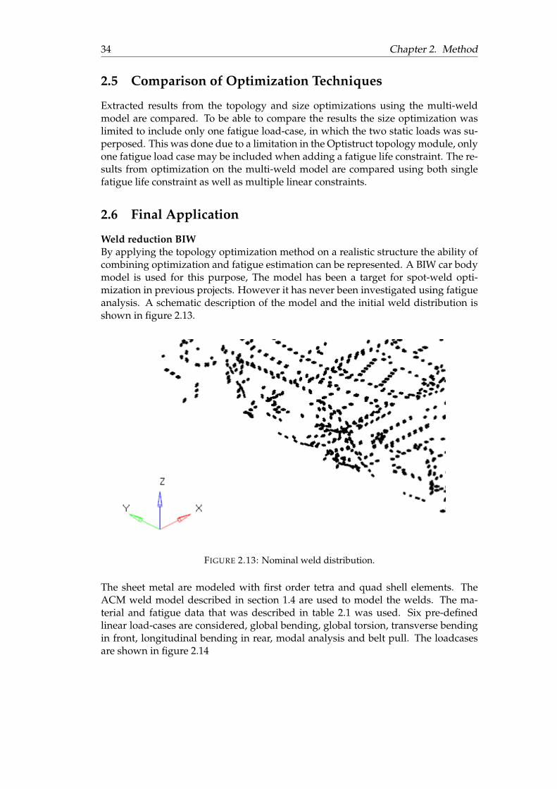
Weld reduction BIWBy applying the topology optimization method on a realistic structure the ability ofcombining optimization and fatigue estimation can be represented. A BIW car bodymodel is used for this purpose, The model has been a target for spot-weld opti-mization in previous projects. However it has never been investigated using fatigueanalysis. A schematic description of the model and the initial weld distribution isshown in figure 2.13.
FIGURE 2.13: Nominal weld distribution.
The sheet metal are modeled with first order tetra and quad shell elements. TheACM weld model described in section 1.4 are used to model the welds. The ma-terial and fatigue data that was described in table 2.1 was used. Six pre-definedlinear load-cases are considered, global bending, global torsion, transverse bendingin front, longitudinal bending in rear, modal analysis and belt pull. The loadcasesare shown in figure 2.14

2.6. Final Application 35
FIGURE 2.14: a) global torsion b ) global bending c ) transverse bend-ing front d ) longitudinal bending rear e ) modal analysis f ) rear belt
pull.
A seventh linear loadcase is added to include the fatigue analysis in the topologyoptimization. The OS software is limited to couple fatigue constraints to one staticloadcase, therefore the global bending is used to compute and constrain the fatiguelife. The global bending load is applied in a simple sinusoidal manner with the loadratio R = −1, the fatigue life is computed using Rupp’s local stress approach de-scribed in section 1.3.2. To investigate the effect of the fatigue constraint the analysisis nominally conducted using only global bending and fatigue constraint, the anal-ysis is then expanded to include all loadcases and all linear constraints (fatigue stilllimited to the global bending loadcase). The constraints is presented in table 2.2.
TABLE 2.2: Linear Constraints for BIW topology optimization.
Constraint Number Description Constraint. [%]1. First torsional mode [Hz] 98.782. First bending mode [Hz] 99.103. Front end lateral mode [Hz] 99.614. Steering system Y-mode [Hz] 99.555. Steering system Z-mode [Hz] 98.546. Retractor right displacement [mm] 120.07. Retractor mid displacement [mm] 120.08. Retractor left displacement [mm] 120.09. Anchor outboard right displacement [mm] 120.010. Anchor inboard right displacement [mm] 120.011. Anchor inboard left displacement [mm] 120.012. Anchor outboard left displacement [mm] 120.013. Transverse bending compliance [mm/N] 82.3014. Tunnel bending compliance [mm/N] 86.5315. Rocker bending compliance [mm/N] 77.1616. Fatigue Life [cycles] 93.23


37
Chapter 3
Results
3.1 Fatigue verification results
Considering the sheet failure mode described in section 1.3.2 the local equivalentstress was calculated based on the nodal forces from the FE-analysis. To verify thecalculation process forces was extracted from a FE-model and put back into the ana-lytical expressions stated in section 1.3.2, this was formulated in a separate MATLABscript. Considering crack propagation in the sheet metal (failure mode sheet), theequivalent radial stress in equation 1.2 can be plotted in the time domain as shownin figure 3.1. The source of the forces and moments contributing to the stresses isof a simple spot-weld specimen that is subjected to a sinusoidal bending (the CPspecimen was used). Each curve in the figure 3.1 represent the stress at an angle,θ, that has been evaluated. In this case, stress at angles of increment of 10 degreeswere evaluated, resulting into 36 individual curves. The curve that yields the mostdamage according to the Palmgren-Miner Rule and Rainflow counting is chosen tobe considered for fatigue.
FIGURE 3.1: The equivalent radial stresses on a single spot-weld sub-jected to sinusoidal bending.
38 Chapter 3. Results
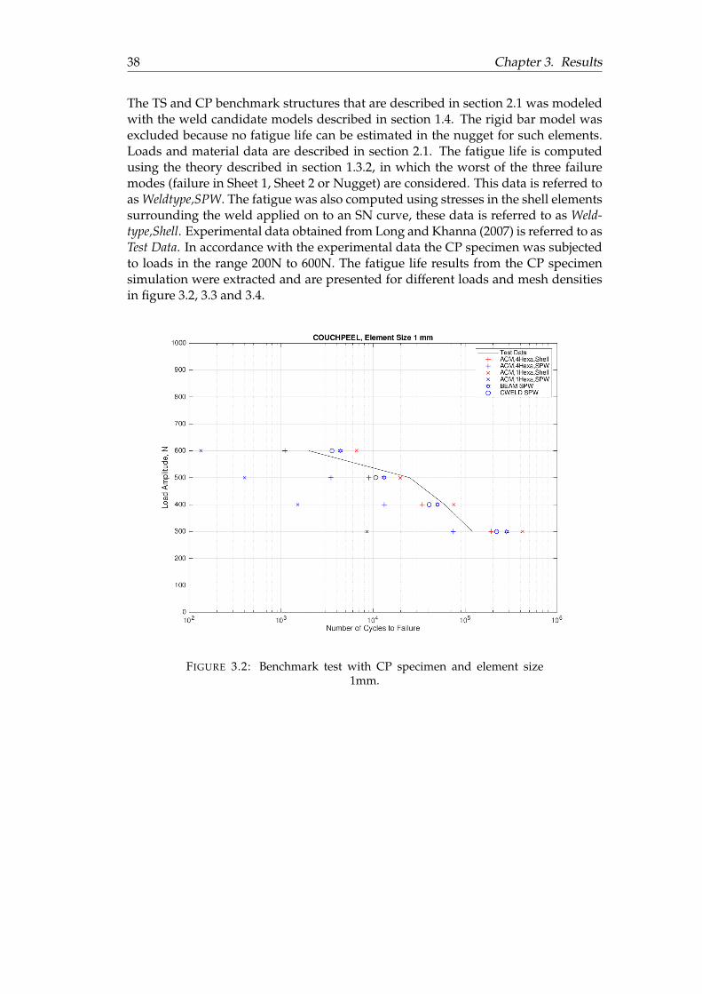
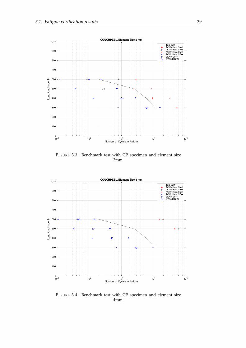
The TS and CP benchmark structures that are described in section 2.1 was modeledwith the weld candidate models described in section 1.4. The rigid bar model wasexcluded because no fatigue life can be estimated in the nugget for such elements.Loads and material data are described in section 2.1. The fatigue life is computedusing the theory described in section 1.3.2, in which the worst of the three failuremodes (failure in Sheet 1, Sheet 2 or Nugget) are considered. This data is referred toas Weldtype,SPW. The fatigue was also computed using stresses in the shell elementssurrounding the weld applied on to an SN curve, these data is referred to as Weld-type,Shell. Experimental data obtained from Long and Khanna (2007) is referred to asTest Data. In accordance with the experimental data the CP specimen was subjectedto loads in the range 200N to 600N. The fatigue life results from the CP specimensimulation were extracted and are presented for different loads and mesh densitiesin figure 3.2, 3.3 and 3.4.
FIGURE 3.2: Benchmark test with CP specimen and element size1mm.
3.1. Fatigue verification results 39
FIGURE 3.3: Benchmark test with CP specimen and element size2mm.
FIGURE 3.4: Benchmark test with CP specimen and element size4mm.
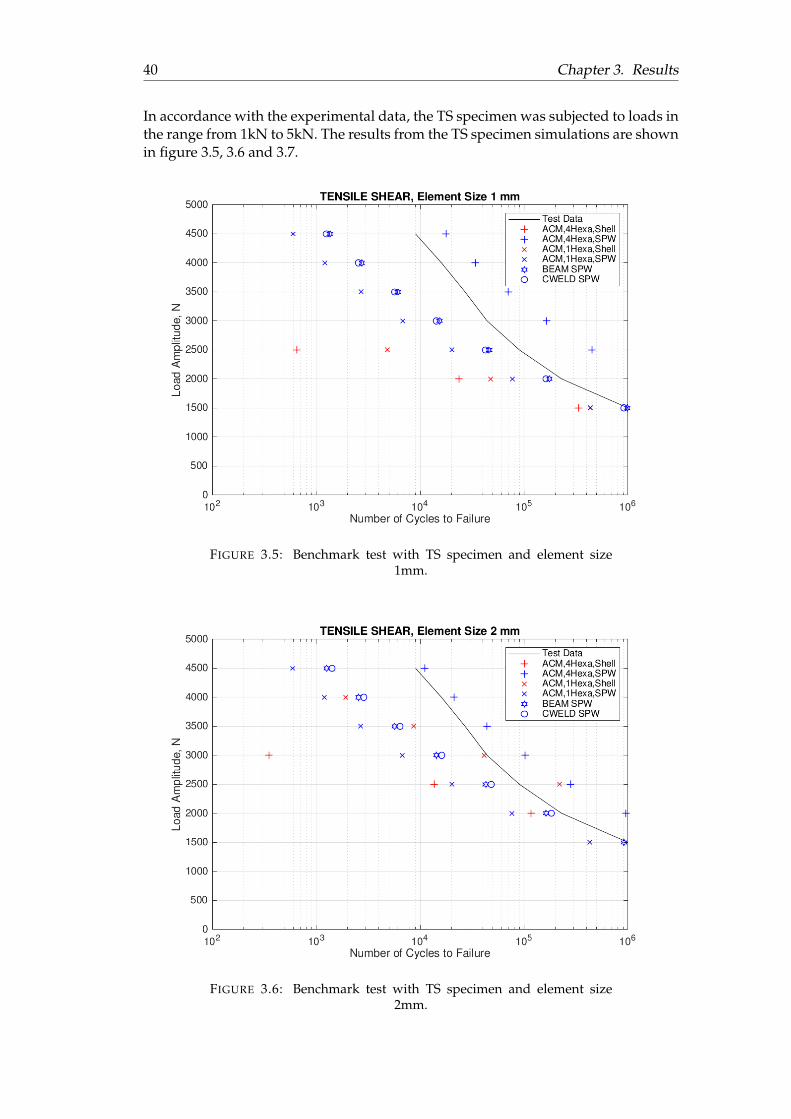
40 Chapter 3. Results
In accordance with the experimental data, the TS specimen was subjected to loads inthe range from 1kN to 5kN. The results from the TS specimen simulations are shownin figure 3.5, 3.6 and 3.7.
FIGURE 3.5: Benchmark test with TS specimen and element size1mm.
FIGURE 3.6: Benchmark test with TS specimen and element size2mm.
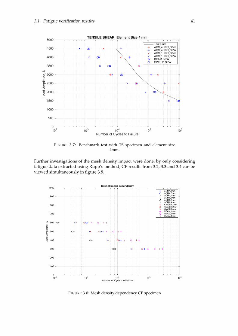
3.1. Fatigue verification results 41
FIGURE 3.7: Benchmark test with TS specimen and element size4mm.
Further investigations of the mesh density impact were done, by only consideringfatigue data extracted using Rupp’s method, CP results from 3.2, 3.3 and 3.4 can beviewed simultaneously in figure 3.8.
FIGURE 3.8: Mesh density dependency CP specimen
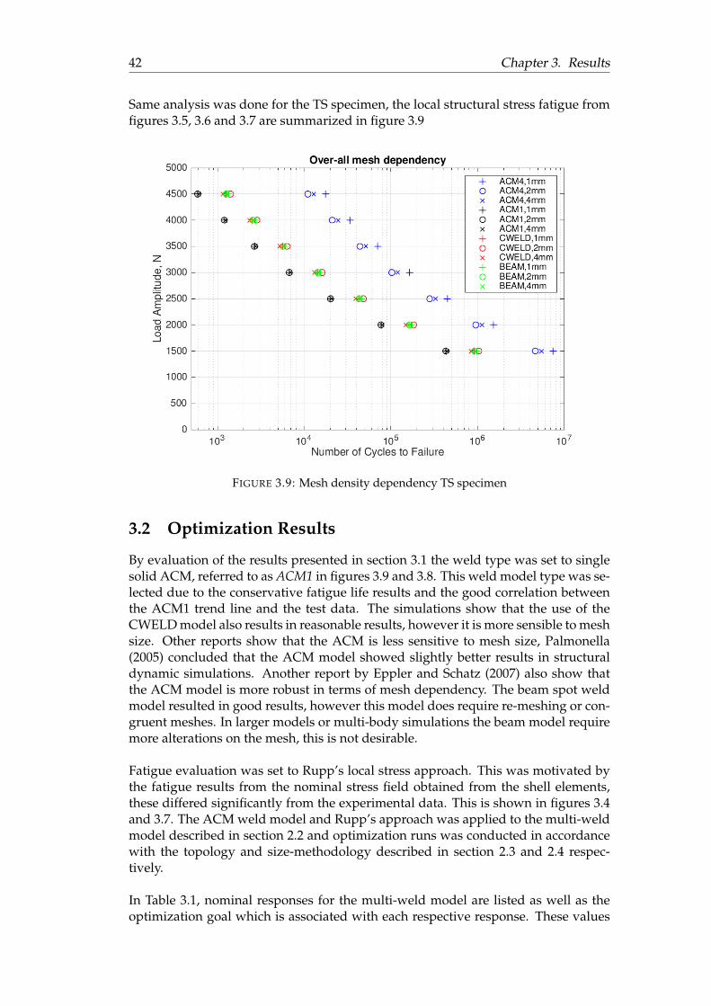
42 Chapter 3. Results
Same analysis was done for the TS specimen, the local structural stress fatigue fromfigures 3.5, 3.6 and 3.7 are summarized in figure 3.9
FIGURE 3.9: Mesh density dependency TS specimen
3.2 Optimization Results
By evaluation of the results presented in section 3.1 the weld type was set to singlesolid ACM, referred to as ACM1 in figures 3.9 and 3.8. This weld model type was se-lected due to the conservative fatigue life results and the good correlation betweenthe ACM1 trend line and the test data. The simulations show that the use of theCWELD model also results in reasonable results, however it is more sensible to meshsize. Other reports show that the ACM is less sensitive to mesh size, Palmonella(2005) concluded that the ACM model showed slightly better results in structuraldynamic simulations. Another report by Eppler and Schatz (2007) also show thatthe ACM model is more robust in terms of mesh dependency. The beam spot weldmodel resulted in good results, however this model does require re-meshing or con-gruent meshes. In larger models or multi-body simulations the beam model requiremore alterations on the mesh, this is not desirable.
Fatigue evaluation was set to Rupp’s local stress approach. This was motivated bythe fatigue results from the nominal stress field obtained from the shell elements,these differed significantly from the experimental data. This is shown in figures 3.4and 3.7. The ACM weld model and Rupp’s approach was applied to the multi-weldmodel described in section 2.2 and optimization runs was conducted in accordancewith the topology and size-methodology described in section 2.3 and 2.4 respec-tively.
In Table 3.1, nominal responses for the multi-weld model are listed as well as theoptimization goal which is associated with each respective response. These values
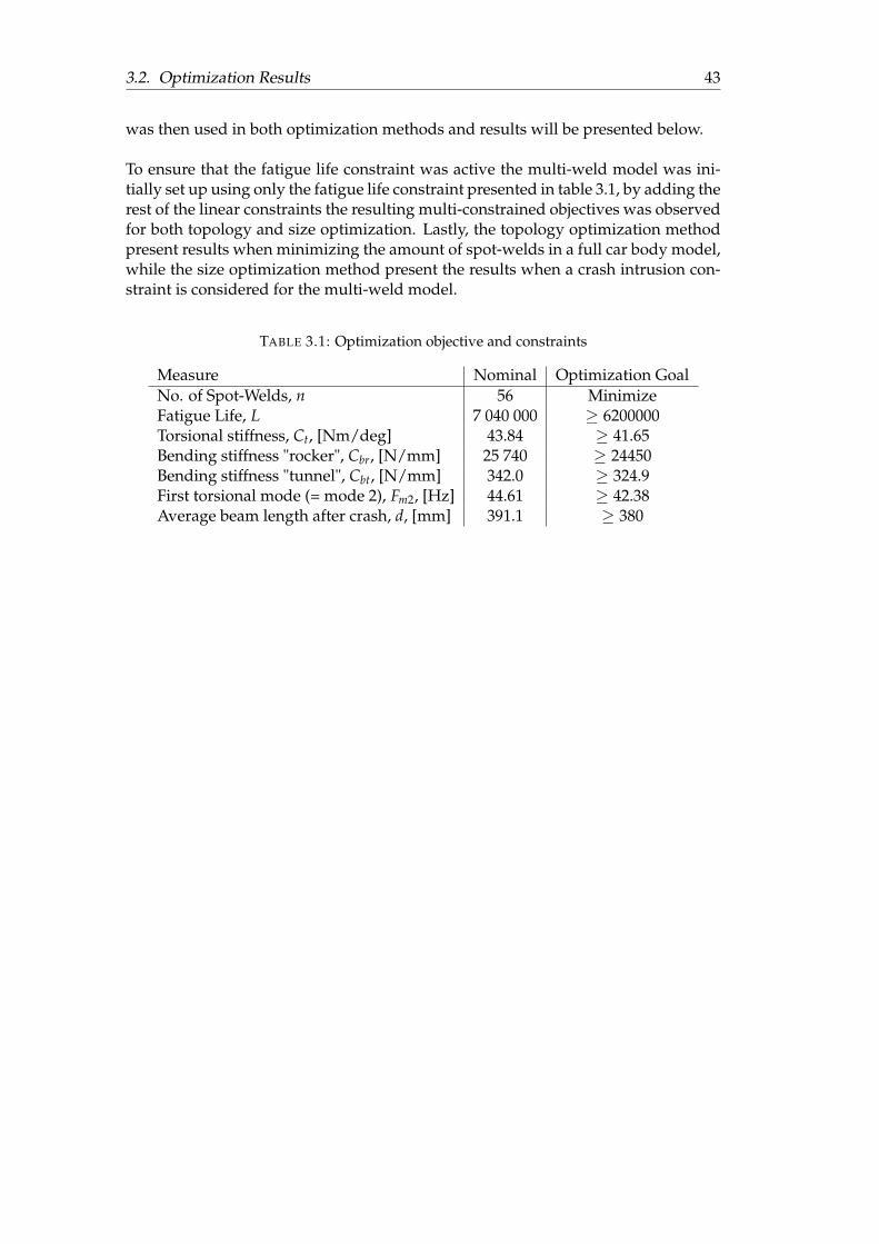
3.2. Optimization Results 43
was then used in both optimization methods and results will be presented below.
To ensure that the fatigue life constraint was active the multi-weld model was ini-tially set up using only the fatigue life constraint presented in table 3.1, by adding therest of the linear constraints the resulting multi-constrained objectives was observedfor both topology and size optimization. Lastly, the topology optimization methodpresent results when minimizing the amount of spot-welds in a full car body model,while the size optimization method present the results when a crash intrusion con-straint is considered for the multi-weld model.
TABLE 3.1: Optimization objective and constraints
Measure Nominal Optimization GoalNo. of Spot-Welds, n 56 MinimizeFatigue Life, L 7 040 000 ≥ 6200000Torsional stiffness, Ct, [Nm/deg] 43.84 ≥ 41.65Bending stiffness "rocker", Cbr, [N/mm] 25 740 ≥ 24450Bending stiffness "tunnel", Cbt, [N/mm] 342.0 ≥ 324.9First torsional mode (= mode 2), Fm2, [Hz] 44.61 ≥ 42.38Average beam length after crash, d, [mm] 391.1 ≥ 380
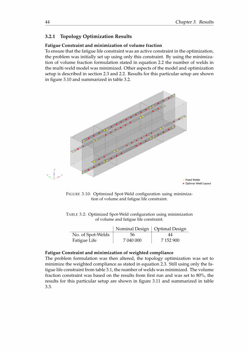
44 Chapter 3. Results
3.2.1 Topology Optimization Results
Fatigue Constraint and minimization of volume fractionTo ensure that the fatigue life constraint was an active constraint in the optimization,the problem was initially set up using only this constraint. By using the minimiza-tion of volume fraction formulation stated in equation 2.2 the number of welds inthe multi-weld model was minimized. Other aspects of the model and optimizationsetup is described in section 2.3 and 2.2. Results for this particular setup are shownin figure 3.10 and summarized in table 3.2.
FIGURE 3.10: Optimized Spot-Weld configuration using minimiza-tion of volume and fatigue life constraint.
TABLE 3.2: Optimized Spot-Weld configuration using minimizationof volume and fatigue life constraint.
Nominal Design Optimal DesignNo. of Spot-Welds 56 44Fatigue Life 7 040 000 7 152 900
Fatigue Constraint and minimization of weighted complianceThe problem formulation was then altered, the topology optimization was set tominimize the weighted compliance as stated in equation 2.3. Still using only the fa-tigue life constraint from table 3.1, the number of welds was minimized. The volumefraction constraint was based on the results from first run and was set to 80%, theresults for this particular setup are shown in figure 3.11 and summarized in table3.3.
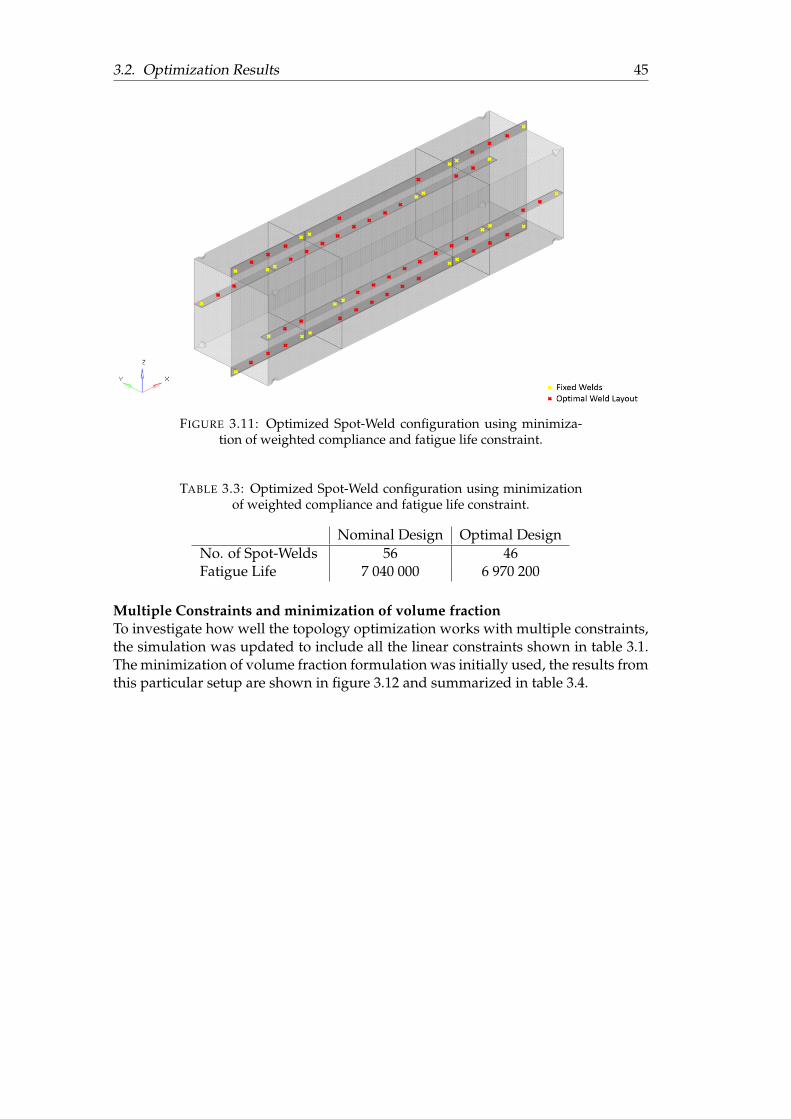
3.2. Optimization Results 45
FIGURE 3.11: Optimized Spot-Weld configuration using minimiza-tion of weighted compliance and fatigue life constraint.
TABLE 3.3: Optimized Spot-Weld configuration using minimizationof weighted compliance and fatigue life constraint.
Nominal Design Optimal DesignNo. of Spot-Welds 56 46Fatigue Life 7 040 000 6 970 200
Multiple Constraints and minimization of volume fractionTo investigate how well the topology optimization works with multiple constraints,the simulation was updated to include all the linear constraints shown in table 3.1.The minimization of volume fraction formulation was initially used, the results fromthis particular setup are shown in figure 3.12 and summarized in table 3.4.
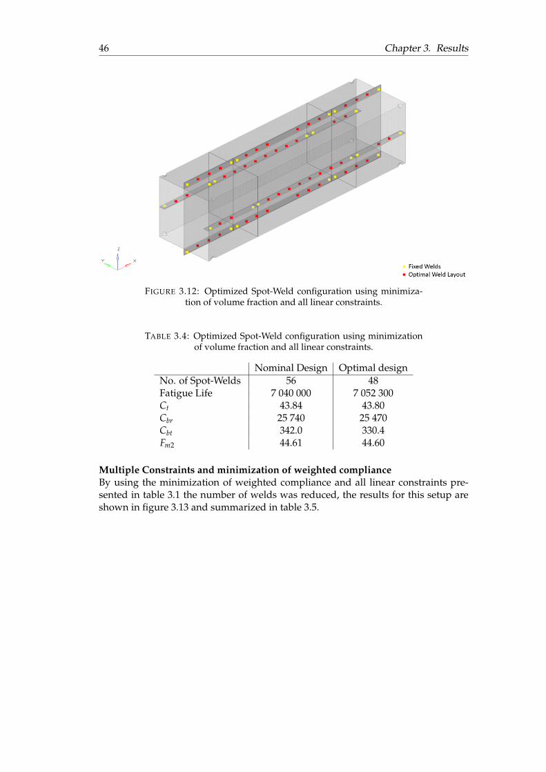
46 Chapter 3. Results
FIGURE 3.12: Optimized Spot-Weld configuration using minimiza-tion of volume fraction and all linear constraints.
TABLE 3.4: Optimized Spot-Weld configuration using minimizationof volume fraction and all linear constraints.
Nominal Design Optimal designNo. of Spot-Welds 56 48Fatigue Life 7 040 000 7 052 300Ct 43.84 43.80Cbr 25 740 25 470Cbt 342.0 330.4Fm2 44.61 44.60
Multiple Constraints and minimization of weighted complianceBy using the minimization of weighted compliance and all linear constraints pre-sented in table 3.1 the number of welds was reduced, the results for this setup areshown in figure 3.13 and summarized in table 3.5.
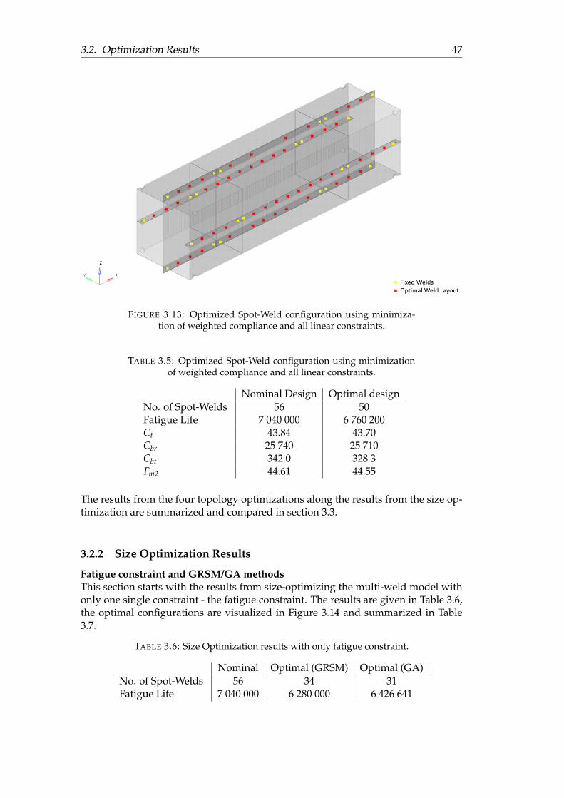
3.2. Optimization Results 47
FIGURE 3.13: Optimized Spot-Weld configuration using minimiza-tion of weighted compliance and all linear constraints.
TABLE 3.5: Optimized Spot-Weld configuration using minimizationof weighted compliance and all linear constraints.
Nominal Design Optimal designNo. of Spot-Welds 56 50Fatigue Life 7 040 000 6 760 200Ct 43.84 43.70Cbr 25 740 25 710Cbt 342.0 328.3Fm2 44.61 44.55
The results from the four topology optimizations along the results from the size op-timization are summarized and compared in section 3.3.
3.2.2 Size Optimization Results
Fatigue constraint and GRSM/GA methodsThis section starts with the results from size-optimizing the multi-weld model withonly one single constraint - the fatigue constraint. The results are given in Table 3.6,the optimal configurations are visualized in Figure 3.14 and summarized in Table3.7.
TABLE 3.6: Size Optimization results with only fatigue constraint.
Nominal Optimal (GRSM) Optimal (GA)No. of Spot-Welds 56 34 31Fatigue Life 7 040 000 6 280 000 6 426 641
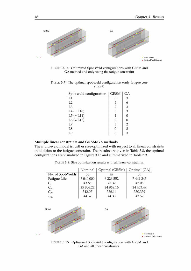
48 Chapter 3. Results
FIGURE 3.14: Optimized Spot-Weld configurations with GRSM andGA method and only using the fatigue constraint
TABLE 3.7: The optimal spot-weld configuration (only fatigue con-straint)
Spot-weld configuration GRSM GAL1 3 3L2 5 6L3 2 3L4 (= L10) 3 3L5 (= L11) 4 0L6 (= L12) 2 0L7 3 2L8 0 8L9 3 3
Multiple linear constraints and GRSM/GA methodsThe multi-weld model is further size-optimized with respect to all linear constraintsin addition to the fatigue constraint. The results are given in Table 3.8, the optimalconfigurations are visualized in Figure 3.15 and summarized in Table 3.9.
TABLE 3.8: Size optimization results with all linear constraints.
Nominal Optimal (GRSM) Optimal (GA)No. of Spot-Welds 56 42 35Fatigue Life 7 040 000 6 226 552 7 449 345Ct 43.85 43.32 42.05Cbr 25 806.22 24 968.16 24 453.49Cbt 342.07 336.14 330.339Fm2 44.57 44.33 43.52
FIGURE 3.15: Optimized Spot-Weld configuration with GRSM andGA and all linear constraints.
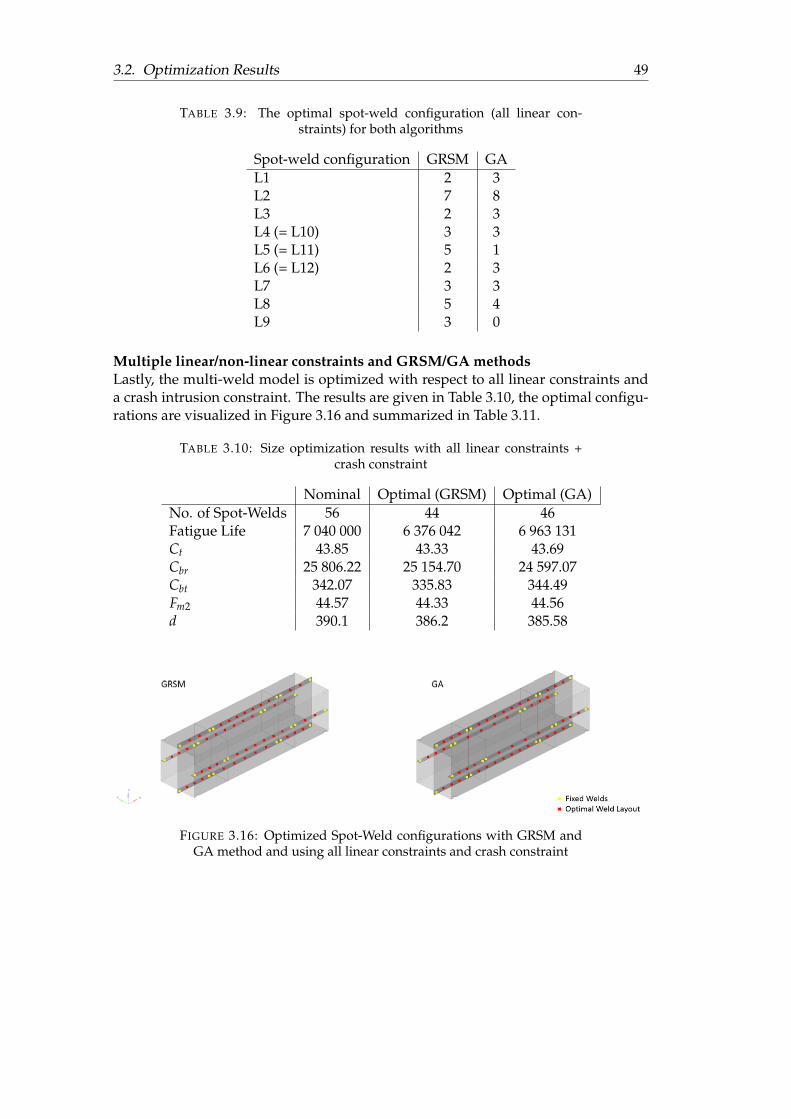
3.2. Optimization Results 49
TABLE 3.9: The optimal spot-weld configuration (all linear con-straints) for both algorithms
Spot-weld configuration GRSM GAL1 2 3L2 7 8L3 2 3L4 (= L10) 3 3L5 (= L11) 5 1L6 (= L12) 2 3L7 3 3L8 5 4L9 3 0
Multiple linear/non-linear constraints and GRSM/GA methodsLastly, the multi-weld model is optimized with respect to all linear constraints anda crash intrusion constraint. The results are given in Table 3.10, the optimal configu-rations are visualized in Figure 3.16 and summarized in Table 3.11.
TABLE 3.10: Size optimization results with all linear constraints +crash constraint
Nominal Optimal (GRSM) Optimal (GA)No. of Spot-Welds 56 44 46Fatigue Life 7 040 000 6 376 042 6 963 131Ct 43.85 43.33 43.69Cbr 25 806.22 25 154.70 24 597.07Cbt 342.07 335.83 344.49Fm2 44.57 44.33 44.56d 390.1 386.2 385.58
FIGURE 3.16: Optimized Spot-Weld configurations with GRSM andGA method and using all linear constraints and crash constraint

50 Chapter 3. Results
TABLE 3.11: Optimal spot-weld configuration (all linear + crash) forboth algorithms
Spot-weld configuration GRSM GAL1 2 3L2 7 7L3 2 3L4 (= L10) 3 3L5 (= L11) 6 4L6 (= L12) 2 3L7 3 3L8 5 7L9 3 3
For comparison purposes the results from both the GRSM and GA methods are pre-sented together with the results extracted from the topology optimization in section3.3.
Validation of Response Surfaces used by the GA methodSince the results from the GA (see third column of table 3.6, 3.8 and 3.10) are basedon a response surface, the given optimal points have to be validated with the actualsimulation model shown in table 3.12. Note that, table 3.12 presents the valueswhen the GA configurations shown in table 3.7, 3.9 and 3.11 are implemented in theoriginal FEM-model and solved by Opistruct/Radioss.
TABLE 3.12: Responses of the suggested optimal design validated inthe simulation model
L Ct Cbr Cbt Fm2 dGA (only fatigue) 568 945 - - - - -GA (all linear) 125 332 41.67 22 362.42 325.30 43.89 -GA (linear + crash) 5 648 379 43.78 24 695.11 342.13 44.54 376.03
Using the approximated results given by table 3.6, 3.8 and 3.10 and the validatedresults from table 3.12, the relative difference ( GAresults−FEMresults
Garesults) is shown between
the responses given from the response surface and the validated design point. Seetable 3.13.
TABLE 3.13: Relative difference between the responses given fromthe response surface (Kriging) and the actual simulated design point
L− rel Ct − rel Cbr − rel Cbt − rel Fm2 − rel d-relGA (only fatigue) −91.2% - - - - -GA (all linear cases) −98.3% −1.95% −8.3% −1.42% −0.8% -GA (linear + crash) −19.1% −1.7% −0.4% −0.7% ≈ 0% −2.4%
In addition to the Kriging models used as the response surfaces for the GA method,RBF models and least square regression models were also created. All three weremeasured on how well observed outcomes (fatigue response) are replicated by re-spective model by the R-Squared definition. A validation matrix consisting of 20randomly chosen design points (separate from the design points creating the re-sponse surfaces) is used for comparison. See Table 3.14.
3.3. Comparison of optimization results 51
TABLE 3.14: Diagnostics of different response surfaces in terms ofR-Square. Based on the fatigue response.
R-Square (R2)Kriging 0.764Full Quadratic Regression 0.599Radial Basis Function 0.569
3.3 Comparison of optimization results
The results from the topology and size optimization using the multi-weld model wascompared to better understand the strengths and weaknesses using different meth-ods. The comparison including all optimization simulations (excluding the crashconstraint) is shown in table 3.15.
TABLE 3.15: Comparison of optimization results
Opt. Meth Const. CPU time No. of welds FatigueSize, GRSM Fatigue 6.70hrs 34 6 280 000Size, GA Fatigue 6.70hrs 31 6 426 641Topology, min. vol. frac. Fatigue 0.12hrs 44 7 152 900Topology, min. weighted comp. Fatigue 0.07hrs 46 6 970 200Size, GRSM All linear 13.0hrs 44 6 376 042Size, GA All linear 13.3hrs 46 6 963131Topology, min. vol. frac. All linear 0.44hrs 48 7 052 300Topology, min. weighted comp. All linear 0.06hrs 50 6 760 200
The results from the topology optimization on the BIW and the size optimization in-cluding the crash constraint must be analyzed independently, the size optimizationare too computationally expensive to apply to the BIW model and topology opti-mization is strictly limited to linear load-cases.
3.4 Final Application
By reviewing the results from the comparison of the optimization methods, it isclear that the size optimization consequently render better designs. However it isimmensely more time demanding and not suitable for analysis of large structures.Therefore the topology optimization was applied to a full BIW model supplied byCombitech, due to the more rapid convergence using weighted compliance this for-mulation was used. Other aspects of the simulation setup are defined in section 2.5.The simulation was initially conducted using only fatigue constraints shown in table2.2, the simulation was then conducted using all linear constraints in table 2.2. Theresults are visualized in figure 3.17 a) and b). The results are also summarized intables 3.16 and 3.17.
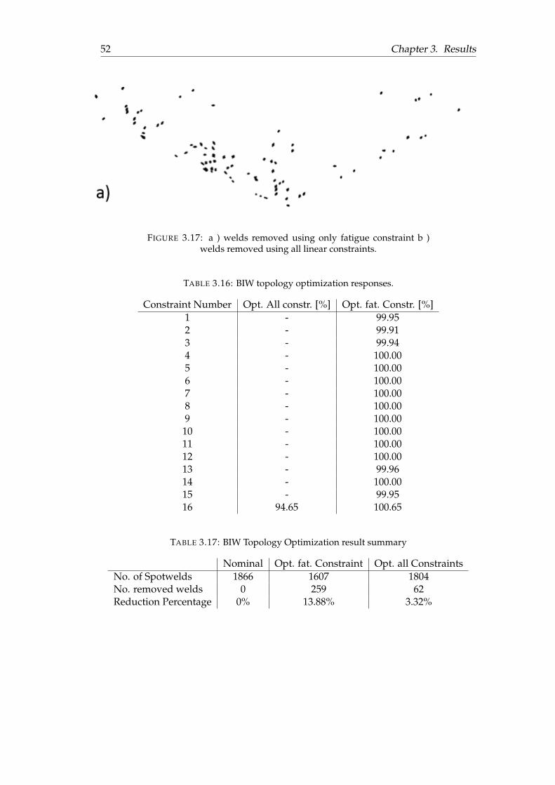
52 Chapter 3. Results
FIGURE 3.17: a ) welds removed using only fatigue constraint b )welds removed using all linear constraints.
TABLE 3.16: BIW topology optimization responses.
Constraint Number Opt. All constr. [%] Opt. fat. Constr. [%]1 - 99.952 - 99.913 - 99.944 - 100.005 - 100.006 - 100.007 - 100.008 - 100.009 - 100.0010 - 100.0011 - 100.0012 - 100.0013 - 99.9614 - 100.0015 - 99.9516 94.65 100.65
TABLE 3.17: BIW Topology Optimization result summary
Nominal Opt. fat. Constraint Opt. all ConstraintsNo. of Spotwelds 1866 1607 1804No. removed welds 0 259 62Reduction Percentage 0% 13.88% 3.32%
53
Chapter 4
Discussion
4.1 Regarding the Fatigue Results
The fatigue life results from the single weld models show that the beam, CWELDand ACM model in combination with Rupp’s local stress approach all generate fea-sible results. The fatigue results computed using the nominal stress field show poorcorrelation and high sensitivity to mesh size. The fatigue results are linear solutionsand therefore bounded to elastic and small-deformation behavior of the material, theresults are also based on the assumption that no fatigue limit is reached. The fatiguelife evaluation method used in this thesis should be applicable to brittle fracture,high-cycle fatigue, and high-speed impact failure of spot welds in which plasticityis contained by a large elastic stress field. For low-cycle fatigue and ultimate fail-ure of spot welds in which plasticity or large deformation may prevail, the resultsare hardly applicable, although they will not necessarily always fail. welding im-perfection, material heterogeneity, residual stress, and other welding-related factorshave not been considered here. It should also be noted that the material parame-ters used for the FE models of the benchmark specimens may not coincide with theones in the actual fatigue testing of Long. Long mentioned which steel type he usedfor his fatigue testing, namely HSLA340Y with the ultimate tensile strength of 448.5MPa and a yield strength of 369.2 MPa. However the fatigue material parameterswere never explicitly mentioned by him. Instead, in this thesis, the material param-eters were taken from an independent source (NCode material library), a HSLA380weld nugget with a yield strength of 320 MPa and and a ultimate tensile strength of484 MPa was used. The fatigue data may differ between these. Considering thesesources of error and by looking at the results in figure 3.2 to 3.7, the spot-weld fa-tigue model according to Rupp still correspond well with the actual test data. Thesimulated data and experimental data show correlation in terms of a common trendin fatigue life, the simulated trend-lines are somewhat shifted on the log(N) axis.
The overall trend for Rupp’s approach for the coach peel specimen is that it seem toconsistently give conservative results, no matter what spot-weld FE model is used.This also applies to the tensile shear specimen, although there is an anomaly wherethe ACM4 model slightly overestimates the fatigue life. The fatigue estimation byjust directly applying the S-N onto the shell-element stress behaves the opposite.The spot-welds modeled as beams are basically infeasible to use for the shell el-ement approach. There will always be an stress-concentration at the point wherethe 1D element connect to the shell elements due to extremely small surfaces beingloaded.
Going through figure 3.2 to 3.7, it is observed that there is minimal mesh dependencyon Rupp’s approach relative to the shell element behavior. This makes sense since
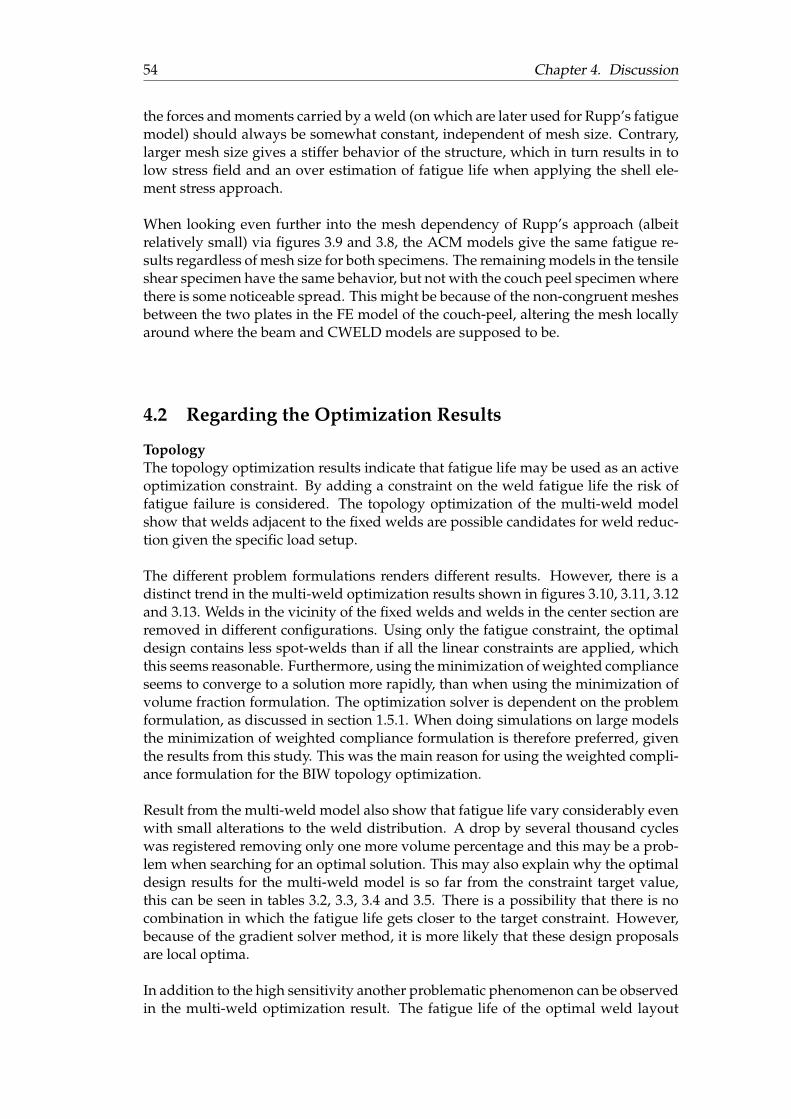
54 Chapter 4. Discussion
the forces and moments carried by a weld (on which are later used for Rupp’s fatiguemodel) should always be somewhat constant, independent of mesh size. Contrary,larger mesh size gives a stiffer behavior of the structure, which in turn results in tolow stress field and an over estimation of fatigue life when applying the shell ele-ment stress approach.
When looking even further into the mesh dependency of Rupp’s approach (albeitrelatively small) via figures 3.9 and 3.8, the ACM models give the same fatigue re-sults regardless of mesh size for both specimens. The remaining models in the tensileshear specimen have the same behavior, but not with the couch peel specimen wherethere is some noticeable spread. This might be because of the non-congruent meshesbetween the two plates in the FE model of the couch-peel, altering the mesh locallyaround where the beam and CWELD models are supposed to be.
4.2 Regarding the Optimization Results
TopologyThe topology optimization results indicate that fatigue life may be used as an activeoptimization constraint. By adding a constraint on the weld fatigue life the risk offatigue failure is considered. The topology optimization of the multi-weld modelshow that welds adjacent to the fixed welds are possible candidates for weld reduc-tion given the specific load setup.
The different problem formulations renders different results. However, there is adistinct trend in the multi-weld optimization results shown in figures 3.10, 3.11, 3.12and 3.13. Welds in the vicinity of the fixed welds and welds in the center section areremoved in different configurations. Using only the fatigue constraint, the optimaldesign contains less spot-welds than if all the linear constraints are applied, whichthis seems reasonable. Furthermore, using the minimization of weighted complianceseems to converge to a solution more rapidly, than when using the minimization ofvolume fraction formulation. The optimization solver is dependent on the problemformulation, as discussed in section 1.5.1. When doing simulations on large modelsthe minimization of weighted compliance formulation is therefore preferred, giventhe results from this study. This was the main reason for using the weighted compli-ance formulation for the BIW topology optimization.
Result from the multi-weld model also show that fatigue life vary considerably evenwith small alterations to the weld distribution. A drop by several thousand cycleswas registered removing only one more volume percentage and this may be a prob-lem when searching for an optimal solution. This may also explain why the optimaldesign results for the multi-weld model is so far from the constraint target value,this can be seen in tables 3.2, 3.3, 3.4 and 3.5. There is a possibility that there is nocombination in which the fatigue life gets closer to the target constraint. However,because of the gradient solver method, it is more likely that these design proposalsare local optima.
In addition to the high sensitivity another problematic phenomenon can be observedin the multi-weld optimization result. The fatigue life of the optimal weld layout
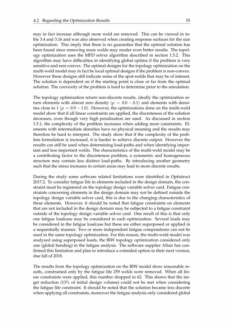
4.2. Regarding the Optimization Results 55
may in fact increase although more weld are removed. This can be viewed in ta-ble 3.4 and 3.16 and was also observed when creating response surfaces for the sizeoptimization. This imply that there is no guaranties that the optimal solution hasbeen found since removing more welds may render even better results. The topol-ogy optimization uses the MFD solver algorithm described in section 1.5.2. Thisalgorithm may have difficulties in identifying global optima if the problem is verysensitive and non-convex. The optimal designs for the topology optimization on themulti-weld model may in fact be local optimal designs if the problem is non-convex.However these designs still indicate some of the spot-welds that may be of interest.The solution is dependent on if the starting point is close or far from the optimalsolution. The convexity of the problem is hard to determine prior to the simulation.
The topology optimization return non-discrete results, ideally the optimization re-turn elements with almost zero density (ρ = 0.0 − 0.1) and elements with densi-ties close to 1 (ρ = 0.9− 1.0). However, the optimizations done on the multi-weldmodel show that if all linear constraints are applied, the discreteness of the solutiondecreases, even though very high penalization are used. As discussed in section1.5.1, the complexity of the problem increases when adding more constraints. El-ements with intermediate densities have no physical meaning and the results maytherefore be hard to interpret. The study show that if the complexity of the prob-lem formulation is increased, it is harder to achieve discrete output. However theresults can still be used when determining load-paths and when identifying impor-tant and less important welds. The characteristics of the multi-weld model may bea contributing factor to the discreteness problem, a symmetric and homogeneousstructure may contain less distinct load-paths. By introducing another geometrysuch that the stress increases in certain areas may lead to more discrete results.
During the study some software related limitations were identified in Optistruct2017.2. To consider fatigue life in elements included in the design domain, the con-straint must be registered on the topology design variable solver card. Fatigue con-straints concerning elements in the design domain may not be defined outside thetopology design variable solver card, this is due to the changing characteristics ofthese elements. However, it should be noted that fatigue constraints on elementsthat are not included in the design domain may be subjected to a fatigue constraintoutside of the topology design variable solver card. One result of this is that onlyone fatigue loadcase may be considered in each optimization. Several loads maybe considered in the fatigue loadcase but these are either superposed or applied ina sequentially manner. Two or more independent fatigue computations can not beused in the same topology optimization. For this reason, the multi-weld model wasanalyzed using superposed loads, the BIW topology optimization considered onlyone (global bending) in the fatigue analysis. The software supplier Altair has con-firmed this limitation and plan to introduce a extended option in their next version,due fall of 2018.
The results from the topology optimization on the BIW model show reasonable re-sults, constrained only by the fatigue life 259 welds were removed. When all lin-ear constraints were applied, this number dropped to 62. This shows that the tar-get reduction (13% of initial design volume) could not be met when consideringthe fatigue life constraint. It should be noted that the solution became less discretewhen applying all constraints, moreover the fatigue analysis only considered global
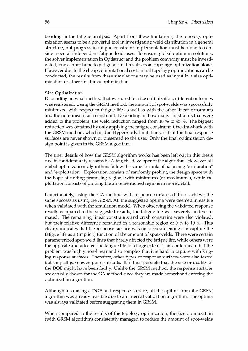
56 Chapter 4. Discussion
bending in the fatigue analysis. Apart from these limitations, the topology opti-mization seems to be a powerful tool in investigating weld distribution in a generalstructure, but progress in fatigue constraint implementation must be done to con-sider several independent fatigue loadcases. To ensure global optimum solutions,the solver implementation in Optistruct and the problem convexity must be investi-gated, one cannot hope to get good final results from topology optimization alone.However due to the cheap computational cost, initial topology optimizations can beconducted, the results from these simulations may be used as input in a size opti-mization or other fine tuned optimization.
Size OptimizationDepending on what method that was used for size optimization, different outcomeswas registered. Using the GRSM method, the amount of spot-welds was successfullyminimized with respect to fatigue life as well as with the other linear constraintsand the non-linear crash constraint. Depending on how many constraints that wereadded to the problem, the weld reduction ranged from 18 % to 45 %. The biggestreduction was obtained by only applying the fatigue constraint. One drawback withthe GRSM method, which is due HyperStudy limitations, is that the final responsesurfaces are never shown or presented to the user. Only the final optimization de-sign point is given in the GRSM algorithm.
The finer details of how the GRSM algorithm works has been left out in this thesisdue to confidentiality reasons by Altair, the developer of the algorithm. However, allglobal optimizations algorithms follow the same formula of balancing "exploration"and "exploitation". Exploration consists of randomly probing the design space withthe hope of finding promising regions with minimums (or maximums), while ex-ploitation consists of probing the aforementioned regions in more detail.
Unfortunately, using the GA method with response surfaces did not achieve thesame success as using the GRSM. All the suggested optima were deemed infeasiblewhen validated with the simulation model. When observing the validated responseresults compared to the suggested results, the fatigue life was severely underesti-mated. The remaining linear constraints and crash constraint were also violated,but their relative difference remained in a reasonable region of 0 % to 10 %. Thisclearly indicates that the response surface was not accurate enough to capture thefatigue life as a (implicit) function of the amount of spot-welds. There were certainparameterized spot-weld lines that barely affected the fatigue life, while others werethe opposite and affected the fatigue life to a large extent. This could mean that theproblem was highly non-linear and so complex that it is hard to capture with Krig-ing response surfaces. Therefore, other types of response surfaces were also testedbut they all gave even poorer results. It is thus possible that the size or quality ofthe DOE might have been faulty. Unlike the GRSM method, the response surfacesare actually shown for the GA method since they are made beforehand entering theoptimization algorithm.
Although also using a DOE and response surface, all the optima from the GRSMalgorithm was already feasible due to an internal validation algorithm. The optimawas always validated before suggesting them in GRSM.
When compared to the results of the topology optimization, the size optimization(with GRSM algorithm) consistently managed to reduce the amount of spot-welds
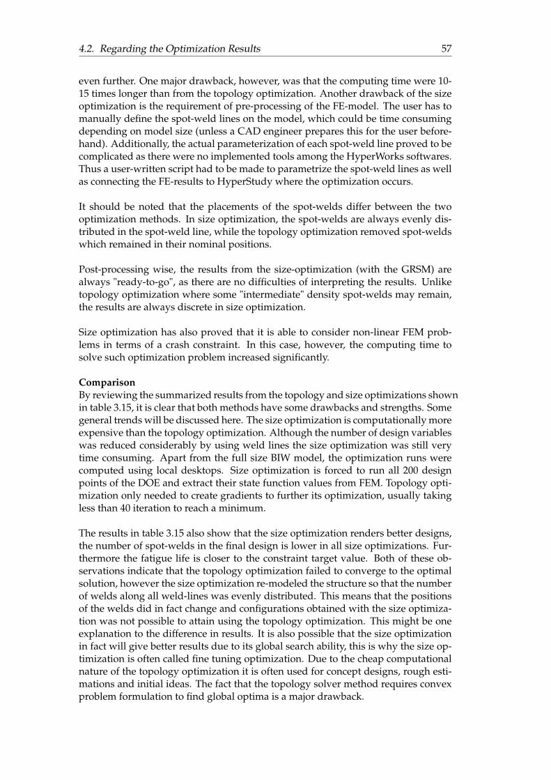
4.2. Regarding the Optimization Results 57
even further. One major drawback, however, was that the computing time were 10-15 times longer than from the topology optimization. Another drawback of the sizeoptimization is the requirement of pre-processing of the FE-model. The user has tomanually define the spot-weld lines on the model, which could be time consumingdepending on model size (unless a CAD engineer prepares this for the user before-hand). Additionally, the actual parameterization of each spot-weld line proved to becomplicated as there were no implemented tools among the HyperWorks softwares.Thus a user-written script had to be made to parametrize the spot-weld lines as wellas connecting the FE-results to HyperStudy where the optimization occurs.
It should be noted that the placements of the spot-welds differ between the twooptimization methods. In size optimization, the spot-welds are always evenly dis-tributed in the spot-weld line, while the topology optimization removed spot-weldswhich remained in their nominal positions.
Post-processing wise, the results from the size-optimization (with the GRSM) arealways "ready-to-go", as there are no difficulties of interpreting the results. Unliketopology optimization where some "intermediate" density spot-welds may remain,the results are always discrete in size optimization.
Size optimization has also proved that it is able to consider non-linear FEM prob-lems in terms of a crash constraint. In this case, however, the computing time tosolve such optimization problem increased significantly.
ComparisonBy reviewing the summarized results from the topology and size optimizations shownin table 3.15, it is clear that both methods have some drawbacks and strengths. Somegeneral trends will be discussed here. The size optimization is computationally moreexpensive than the topology optimization. Although the number of design variableswas reduced considerably by using weld lines the size optimization was still verytime consuming. Apart from the full size BIW model, the optimization runs werecomputed using local desktops. Size optimization is forced to run all 200 designpoints of the DOE and extract their state function values from FEM. Topology opti-mization only needed to create gradients to further its optimization, usually takingless than 40 iteration to reach a minimum.
The results in table 3.15 also show that the size optimization renders better designs,the number of spot-welds in the final design is lower in all size optimizations. Fur-thermore the fatigue life is closer to the constraint target value. Both of these ob-servations indicate that the topology optimization failed to converge to the optimalsolution, however the size optimization re-modeled the structure so that the numberof welds along all weld-lines was evenly distributed. This means that the positionsof the welds did in fact change and configurations obtained with the size optimiza-tion was not possible to attain using the topology optimization. This might be oneexplanation to the difference in results. It is also possible that the size optimizationin fact will give better results due to its global search ability, this is why the size op-timization is often called fine tuning optimization. Due to the cheap computationalnature of the topology optimization it is often used for concept designs, rough esti-mations and initial ideas. The fact that the topology solver method requires convexproblem formulation to find global optima is a major drawback.
58 Chapter 4. Discussion
4.3 Further Work
In this thesis, the structural stress approach to spot-weld fatigue proposed by Rupp(1995) was considered. There are more fatigue models available that may be of in-terest to investigate in future studies. Swellam (1991) and Sheppard (1993) managedto individually develop their own spot-weld fatigue models derived based on lin-ear elastic fracture mechanics (LEFM) assumptions. Kang (2000) summarized the fa-tigue life according to Swellam, Sheppard as well as Rupp’s approach and presentedhow they fared against fatigue data. The results were promising, however, apply-ing the LEFM approaches to this thesis would be too time consuming since thesemodels were not implemented into the FE-solver, unlike Rupp’s approach which iscommonly implemented in most FE-softwares.
Like the fatigue models for spot-welds, there are plenty of other FE-models of spot-welds in addition to the ones presented in this thesis. One FE-model in particularof interest, is the rigid spider model consisting of an umbrella/spider-like configu-ration of rigid bars. The spider model was investigated by Andersson and Deleskog(2014) as a part of their thesis toward Volvo Cars.
For both topology and size optimization, several search algorithms schemes were of-fered by Hyperworks but were later decided to be left out of this thesis. In additionto MFD (method of feasible directions), other gradient-based schemes were read-ily available such as Sequential Quadratic Programming (SQP) and Dual Optimizerbased on separate convex approximation (DUAL). Although only global search al-gorithms were applied for the size optimization, it is indeed possible to use gradient-based algorithms. However, since gradient-based algorithms cannot handle discretedesign variables as presented in this thesis with size optimization, they have to beconverted in to continuous ones representing the distance between the spot-weldswithin a weld line. The user-written script that was used to parameterize the spot-weld lines has to be then rewritten as how d’Ippolito et al. (2008) parameterizedtheirs.
The optimization in this thesis has so far only managed to apply a deterministicmindset of deciding what spot-weld configuration is the optimized one. There arepossibilities of taking this one step further by applying a probabilistic design choice.There are a variety of tools for making reliable decisions with the consideration ofuncertainties associated with the simulation model. An uncertainty analysis has tobe made, through which quantifying the impact of the uncertainty associated withthe system input is on the system output (the state functions) by identifying the lat-ter probabilistic characteristics. By having this uncertainty analysis in mind, an opti-mization can be made by managing and mitigating the effects of uncertainty on theoutputs. However, applying probabilistic design is computationally intensive. Theoptimization algorithm often involves capturing the probabilistic characteristics ofthe state functions at each individual design point.
59
Chapter 5
Conclusion
To sum up our recommendations and to answer the questions raised in the thesisobjective section the following conclusions were made.
Regarding the weld modeling the ACM weld model is recommended due to,
• ACM does not require congruent meshes and therefore no re-meshing or othermodel alterations is needed.
• Responses and especially spot-weld fatigue show low sensitivity to mesh sizewhen using ACM.
• The ACM model are a relatively better model when simulating structural stiff-ness and dynamic responses.
Regarding the spot-weld fatigue evaluation,
• Fatigue evaluation using nominal stress approach is not recommended due tohigh sensitivity to mesh density and low correlation with simple single weldtest data.
• Rupp’s structural stress approach show reasonable fatigue life results and aretherefore recommended for spot-weld fatigue modeling, although models shouldbe configured with psychical tests to accurately capture fatigue properties.
• Rupp’s approach are limited to high cycle fatigue and linear elastic assump-tions.
Regarding the structural optimization,
• Fatigue life responses show significant sensitivity to spot-weld removal, smallchanges or even single weld removal greatly affect the fatigue response.
• Topology optimization are recommended for large, quick and relatively simplespot-weld optimizations. However, when conducting topology optimizationin the software Optistruct this method are limited to linear elastic and convexproblems. Furthermore, this software are also limited to one fatigue load casewhen optimizing with a fatigue constraint.
• The size optimization are recommended for non-convex, non-linear and smallscale problems. The size optimization is very computationally demanding butworks well for exploratory and fine tuning optimizations. When optimizingin Hyperstudy considering fatigue life we strongly suggest that the GRSMmethod is adapted. Due to its built in validation, the design proposals meetthe stated constraints. The GA method needs more samples to build a reliableresponse surface.

61
Bibliography
Abasi, Babak (2012). “Improving response surface methodology by using artificialneural network and simulated annealing”. In: Expert systems with applications.
Alfredsson, Bo, Per-Lennart Osk Larsson, and Hans Öberg (2017). Testing Techniquesin Solid Mechanics, Course Compendium.
Altair. HyperWorks Help.Andersson, Joel and Jonatan Deleskog (2014). “Fatigue Life and Stiffness of the Spi-
der Spot Weld Model”. In: Master Thesis, Chalmers Applied Mechanics.Bendsoe, M.P. (2004). Topology Optimization. New York: Springer.Castelo, Eduardo (2004). “On Spot Weld Modeling in Vehicle Numerical Simula-
tions”. In: SAE Technical Paper Series 3432, pp. 1,2.d’Ippolito, Roberto et al. (2008). “Multi-disciplinary Optimization of a vehicle spot
weld layout under durability and NVH constraints”. In: International Conferenceon Noise and Vibration Engineering 1, pp. 4111–4125.
Fang, J. (2011). “Weld Modeling with MSC.Nastran”. In: MSC.Software Corporation.Heiserer, Daniel (1999). “High Performance, Process Oriented, Weld Spot Approach”.
In: The university of illinois at Urbana-Champaign.Hobbacher, A.F. (2016). Recommendations for Fatigue Design of Welded Joints and Com-
ponents. Wilhelmshaven, Germany: Springer.Kang, H. (2000). “Evaluation of multiaxial spot weld fatigue parameters for propor-
tional loading”. In: International Journal of Fatigue 2, pp. 691–702.Khanna, Sanjeev (2010). “Fatigue behavior of spot welded joints in steel sheets”. In:
Ford Research Labs.Long, Xin and Sanjeev Khanna (2007). “Fatigue properties and failure characteriza-
tion of spot welded high strength steel sheet”. In: International Journal of Fatigue29, pp. 879–886.
Lundh, Hans (2000). Grundläggande Hållfasthetslära. Stockholm, Sweden.Matsuishi, M. and Tatsuo Endo (1968). “Fatigue of metals subjected to varying stress”.
In: Japan Soc. Mech. Engineering.Nakahara, Yuji (2000). “Method of Fatigue Life estimation for Spot-Welded Struc-
tures”. In: SAE Technical Paper Series 0779.Palmonella, Matteo (2005). “Finite element models of spot welds in structural dy-
namics”. In: Science Direct 83.Pan, J. (2010). Failure mechanisms of advanced welding processes. USA: Woodhead Pub-
lishing Limited.Puchner, Klaus (2006). “Spot Weld Optimization Regarding Stiffness and Fatigue
Using Standard Software”. In: SAE Technical Paper Series 1247.Rupp, Andreas (1995). “Computer Aided Dimensioning of Spot-Welded Automo-
tive Structures”. In: International Congress and Exposition.Ryberg, Ann-Britt and Larsgunnar Nilsson (2016). “Spot weld reduction methods for
automotive structures”. In: Structural and multidisciplinary optimization 53, pp. 923–934.
Sadek, Salar et al. (2017). “An Introduction to Design Optimization”. In: KTH mate-rial.

62 BIBLIOGRAPHY
Sheppard, Sheri (1993). “Estimation of fatigue propagation life in resistance spotwelds”. In: Advances in Fatigue Predictive Techniques 2.
Socie, Darrel (2017). Efatigue. USA.Svanberg, Krister (2017). Optimization. Sweden: KTH.Swellam, M.H. (1991). “A fatigue design parameter for spot welds”. In: The university
of illinois at Urbana-Champaign.Torsten Eppler, Rolf Schatz (2007). “Modeling of spot welds for NVH simulations in
view of refined panel meshes.” In: Master Thesis.Young, Warren (1989). Roark’s Formulas for Stress and Strain. USA: McGraw-Hill.Zoutendijk, G. (1959). “Maximizing a Function in a Convex Region”. In: Journal of
the Royal Statistical Society 21.2, pp. 338–355.


TRITA TRITA-SCI-GRU 2018:219
www.kth.se