Embed Size (px)
Citation preview
SPM Users Guide
Classification Modeling in CART
This guide provides a detailed description of classification modeling in CART.
Title: Classification Modeling in CART
Short Description: This guide provides a detailed description of classification modeling in CART.
Long Description: The main purpose of this guide is to provide a detailed overview of classification
modeling in CART. We will address the full set of options available during the model setup as well as
guide you through all available output reports and displays. A simple dataset coming from the biomedical
application field will be used to illustrate all of the key concepts.
Salford Systems' CART is the only decision-tree system based on the original CART code developed by
world-renowned Stanford University and University of California at Berkeley statisticians Breiman,
Friedman, Olshen and Stone.
Key Words: CART, Classification and Regression Trees, decision trees, predictive models, data mining

Classification Modeling in CART
2
Copyright, 2016 Salford Systems
Introduction
The main purpose of this guide is to provide a detailed overview of classification modeling in CART. We
will address the full set of options available during the model setup as well as guide you through all
available output reports and displays. A simple dataset coming from the biomedical application field will
be used to illustrate all of the key concepts.
Setting up a Classification Model in CART
Modeling Dataset
We start by walking through a simple classification problem taken from the biomedical literature. The topic
is low birth weight of newborns. The task is to understand the primary factors leading to a baby being
born significantly underweight. The topic is considered important by public health researchers because
low birth weight babies can impose significant burdens and costs on the healthcare system. A cutoff of
2500 grams is typically used to define a low birth weight baby.
The following variables are available:
LOW - Birth weight less than 2500 grams (coded 1 if <2500, 0 otherwise).
AGE - Mother’s age.
FTV - Number of first trimester physician visits.
HT - History of hypertension (coded 1 if present, 0 otherwise).
LWD - Low Mother’s weight at last menstrual period (coded 1 if <110 pounds, 0 otherwise).
PTD - Occurrence of pre-term labor (coded 1 if present, 0 otherwise).
RACE - Mother’s ethnicity (coded 1, 2 or 3).
SMOKE - Smoking during pregnancy (coded 1 if smoked, 0 otherwise).
UI - Uterine irritability (coded 1 if present, 0 otherwise).
As you might guess we are going to explore the possibility that characteristics of the mother, including
demographics, health status, and the mother’s behavior, might influence the probability of a low birth
weight baby.
Begin by looking for the HOSLEM.CSV data file that should be located in your Sample Data folder. You
may consult the generic parts of this manual for a detailed description on how to open datasets for
modeling and related simple steps mentioned below:
Open the HOSLEM.CSV dataset located in the Sample Data folder.

Classification Modeling in CART
3
Copyright, 2016 Salford Systems
33
Press the [Model…] button in the activity window (unless the window is suppressed).
You should now have the Model Setup window opened. In what follows, we describe the purpose of all
individual tabs.
Model Tab
This generic tab is used to set up analysis type, as well as select target and predictors:
Make sure that the Analysis Engine selection box has CART.
Make sure that the Target Type is set to Classification/Logistic Binary.
Change the Sort: selection box to File Order.
Select LOW as the target variable.
Select AGE, RACE, SMOKE, HT, UI, FTV, PTD, and LWD as predictors.
Specify RACE, UI, and FTV as categorical predictors.
Specify AGE, SMOKE, and BWT as auxiliary variables (see below).

Classification Modeling in CART
4
Copyright, 2016 Salford Systems
Target Column
This is where you specify the target variable for the analysis.
MODEL <variable>
Example> MODEL LOW
Model (target and predictors) reset: LOW
Predictor Column
This is where you specify the predictors to be used.
KEEP <variable>, <variable>, …
Example> KEEP AGE, RACE, SMOKE, HT, UI, FTV, PTD, LWD
✓ When the Target Type is set to Classification/Logistic Binary, the target variable will be automatically defined as categorical and appear with the corresponding checkmark at later invocations of the Model Setup. Similarly, the Regression radio button will automatically cancel the categorical status of the target variable. In other words, the specified Target Type determines whether the target is treated as categorical or continuous.

Classification Modeling in CART
5
Copyright, 2016 Salford Systems
55
Categorical Column
This is where you specify which predictors are categorical (nominal or discrete).
CATEGORY <variable>, <variable>, …
Example> CATEGORY FTV, LOW, RACE, UI
CART supports "high-level categorical variables" through its proprietary algorithms that quickly determine
effective splits in spite of the daunting combinatorics of many-valued predictors. This feature is
increasingly important in the presence of character predictors, which in "real world" datasets often have
hundreds or even thousands of levels. When forming a categorical splitter, traditional CART searches all
possible combinations of levels, an approach in which time increases geometrically with the number of
levels. In contrast, CART's high-level categorical algorithm increases linearly with time, yet yields the
optimal split in most situations.
Character variables are implicitly treated as categorical (discrete), so there is no need to "declare" them
categorical. There is no internal limit on the length of character data values (strings). You are limited in
this respect only by the data format you choose (e.g., SAS, text, Excel, etc.).
✓ Character variables (marked by “$” at the end of variable name) will always be treated as categorical and cannot be unchecked.
✓ Occasionally columns stored in an Excel spreadsheet will be tagged as “Character” even though the values in the column are intended to be numeric. If this occurs with your data, refer to the READING DATA section to remedy this problem.
Depending whether a variable is declared as continuous or categorical, CART will search for different
types of splits. Each takes on a unique form.
Continuous splits will always use the following form.
A case goes left if [split-variable] <= [split-value]
A node is partitioned into two children such that the left child receives all the cases with the lower values
of the [split-variable].
Categorical splits will always use the following form.
A case goes left if [split-variable] = [level_i OR …level_j OR … level_k]
In other words, we simply list the values of the splitter that go left (and all other values go right).
One should exercise caution when declaring continuous variables as categorical because a large number of distinct levels may result in significant increases in running times and memory consumption.
Any categorical predictor with a large number of levels can create problems for the model. While there is no hard and fast rule, once a categorical predictor exceeds about 50 levels there are likely to be compelling reasons to try to combine levels until it meets this limit. We show how CART can conveniently do this for you later in the manual (see Introduction to Data Binning).

Classification Modeling in CART
6
Copyright, 2016 Salford Systems
Weight Column
In addition to selecting target and predictor variables, the Model tab allows you to specify a case-
weighting variable.
WEIGHT <variable>
Case weights, which are stored in a variable on the dataset, typically vary from observation to
observation. An observation’s case weight can, in some sense, be thought of as a repetition factor. A
missing, negative or zero case weight causes the observation to be deleted, just as if the target variable
were missing. Case weights may take on fractional values (e.g., 1.5, 27.75, 0.529, 13.001) or whole
numbers (e.g., 1, 2, 10, 100).
To select a variable as the case weight, simply put a checkmark against that variable in the Weight
column.
✓ Case weights do not affect linear combinations in CART Basic, but are otherwise used throughout CART. CART Pro, ProEX, and Ultra include a new linear combination facility that recognizes case weights.
✓ If you are using a test sample contained in a separate dataset, the case weight variable must exist and have the same name in that dataset as in your main (learn sample) dataset.
Aux. Column
This is where you can mark Auxiliary variables.
AUXILIARY <variable>, <variable>, …
Example> AUXILIARY AGE, SMOKE, BWT
Auxiliary variables are variables that are tracked throughout the CART tree but are not necessarily used
as predictors. By marking a variable as Auxiliary, you indicate that you want to be able to retrieve basic
summary statistics for such variables in any node in the CART tree. In our modeling run based on the
HOSLEM.CSV data, we mark AGE, SMOKE and BWT as auxiliary.
Later in this guide, we discuss how to view auxiliary variable distributions on a node-by-node basis.
Setting Focus Class
In classification runs some of the reports generated by CART (gains, prediction success, color-coding,
etc.) have one target class in focus. By default, CART will put the first class it finds in the dataset in
focus. A user can overwrite this by pressing the [Set Focus Class…] button and selecting the desired
class.
Sorting Variable List
The variable list can be sorted either in physical order or alphabetically by changing the Sort: control box.
Depending on the dataset, one of those modes will be preferable, which is usually helpful when dealing
with large variable lists.
Classification Modeling in CART
7
Copyright, 2016 Salford Systems
77
Categorical Tab
The Categorical tab allows you to manage text labels for categorical predictors and it also offers controls
related to how we search for splitters on high-level categorical predictors. The splitter controls are
discussed later as this is a rather technical topic and the defaults work well.
Setting Class Names
CLASS <variable> <value1> = “<label1>”, <value2> = “<label2>”, …
Class names are defined in the Categorical tab. Press [Set Class Names] to get started. In the left
panel, select a variable for which labels are to be defined. If any class labels are currently defined for this
variable, they will appear in the left panel and, if the variable is selected, in the right panel as well (where
they may be altered or deleted). To enter a new class name in the right panel for the selected variable,
define a numeric value (one that will appear in your data) in the "Level" column and its corresponding text
label in the “Class Values for:” column. Repeat for as many class names as necessary for the selected
variable.
You need not define labels for all levels of a categorical variable. A numeric level, which does not have a
class name, will appear in the CART output as it always has, as a number. Also, it is acceptable to define
labels for levels that do not occur in your data. This allows you to define a broad range of class names
for a variable, all of which will be stored in a command script (.CMD file), but only those actually
appearing in the data you are using will be used.
In a classification tree, class names have the greatest use for categorical numeric target variables (i.e., in
a classification tree). For example, for a four-level target variable PARTY, classes such as “Independent,”
“Liberal,” “Conservative,” and “Green” could appear in CART reports and the navigator rather than levels
"1", "2", "3", and "4.” In general, only the first 32 characters of a class name are used, and some text
reports use fewer due to space limitations.

Classification Modeling in CART
8
Copyright, 2016 Salford Systems
In our example we specify the following class names for the target variable LOW and predictor UI. These
labels then will appear in the tree diagrams, the CART text output, and most displays. The setup dialog
appears as follows.
GUI CART users who use class names extensively should consider defining them with commands in a
command file and submitting the command file from the CART notepad once the dataset has been
opened. The CLASS commands must be given before the model is built.
✓ If you use the GUI to define class names and wish to reuse the class names in a future session, save the command log before exiting CART. Cut and paste the CLASS commands appearing in the command log into a new command file.
✓ You can add labels to the target variable AFTER a tree is grown, but these will appear only in the navigator window (not in the text reports). Activate a navigator window, pull down the View menu and select the Assign Class Names… menu item.
High-Level Categorical Predictors BOPTIONS NCLASSES = <n>
BOPTIONS HLC = <n>, <n>
We take great pride in noting that CART is capable of handling categorical predictors with thousands of
levels (given sufficient RAM workspace). However, using such predictors in their raw form is generally not
a good idea. Rather, it is usually advisable to reduce the number of levels by grouping or aggregating
levels, as this will likely yield more reliable predictive models. It is also advisable to impose the HLC
penalty on such variables (from the Model Setup—Penalty tab). These topics are discussed at greater
length later in the manual. In this section we discuss the simple mechanics for handling any HLC
predictors you have decided to use.
For the binary target, high-level categorical predictors pose no special computational problem as exact
short cut solutions are available and the processing time is minimal no matter how many levels there are.
For the multi-class target variable (more than two classes), we know of no similar exact short cut
methods, although research has led to substantial acceleration. HLCs present a computational challenge
because of the sheer number of possible ways to split the data in a node. The number of distinct splits
that can be generated using a categorical predictor with K levels is 2K-1 -1. If K=4, for example, the number
of candidate splits is 7; if K=11, the total is 1,023; if K=21, the number is over one million; and if K=35, the

Classification Modeling in CART
9
Copyright, 2016 Salford Systems
99
number of splits is more than 34 billion! Naïve processing of such problems could take days, weeks,
months, or even years to complete!
To deal more efficiently with high-level categorical (HLC) predictors, CART has an intelligent search
procedure that efficiently approximates the exhaustive split search procedure normally used. The HLC
procedure can radically reduce the number of splits actually tested and still find a near optimal split for a
high-level categorical.
The control option for high-level categorical predictors appears in the Categorical tab as follows.
The settings above indicate that for categorical predictors with 15 or fewer levels we search all possible
splits and are guaranteed to find the overall best partition. For predictors with more than 15 levels we use
intelligent shortcuts that will find very good partitions but may not find the absolute overall best. The
threshold level of 15 for enabling the short-cut intelligent categorical split searches can be increased or
decreased in the Categorical dialog. In the short cut method we conduct “local” searches that are fast but
explore only a limited range of possible splits. The default setting for the number of local splits to search
is around 200. To change this default and thus search more or less intensively, increase or decrease the
search intensity gauge. Our experiments suggest that 200 is a good number to use and that little can be
gained by pushing this above 400. As indicated in the Categorical dialog, a higher number leads to more
intensive and longer searching whereas a lower number leads to faster, less thorough searching. If you
insist on more aggressive searching you should go to the command line.
✓ These controls are only relevant if your target variable has more than two levels. For the two-level binary target (the YES/NO problem), CART has special shortcuts that always work.
There are actually disadvantages to searching too aggressively for the best HLC splitter, as such searches increase the likelihood of overfitting the model to the training data.
Classification Modeling in CART
10
Copyright, 2016 Salford Systems
Force Split tab FORCE ROOT ON <categorical variable> AT <value1>, <value2>, …
FORCE LEFT ON <categorical variable> AT <value1>, <value2>, …
FORCE RIGHT ON <continuous variable> AT <value>
Sometimes, there is a need to override splits that were automatically found by CART, or simply force
alternative splits into a tree. The Force Split tab allows you to define your own split variable and/or split
value at the root node and also any of the child nodes of the root node during the model setup.
✓ Command-line offer more flexible FORCE facility which, in conjunction with the Force Commands pop-up menu available in the Navigator window, allows you to change any split anywhere within the current tree. This is described later in this manual.
Classification Modeling in CART
11
Copyright, 2016 Salford Systems
111
1
Specifying the Root Node Splitter
Press the [Start] button in the Model Setup window to build a CART tree based on the current settings.
Now click on the root node to see detailed split information
CART decided to use PTD as the main splitter; however, LWD while having somewhat smaller
improvement is a good competitor. Suppose you would like to override CART’s decision and force LWD
as the root node splitter.

Classification Modeling in CART
12
Copyright, 2016 Salford Systems
Here is how you can accomplish this:
Go back to the Model Setup window and click on the Force Split tab.
Select the LWD variable in the predictor list on the left.
Press the [Set Root] button; this will place this variable in the Root Node group.
Check the Set Split Value checkbox, and then press the [Change…] button.
In the resulting dialog window, enter the continuous split value of 0.5 and click [OK].
The Force Split tab now should look like this:
Be careful when you set the split value, trying to set a wrong value may result to a degenerate split (all cases go on one side of the split) and will produce a warning.
✓ The Set Split Value step above can be skipped; this will only force the splitter variable while letting CART automatically find the split value for you.
Press the [Start] button and confirm that the root node uses the enforced split by clicking on the root
node in the new Navigator window.
Classification Modeling in CART
13
Copyright, 2016 Salford Systems
131
3
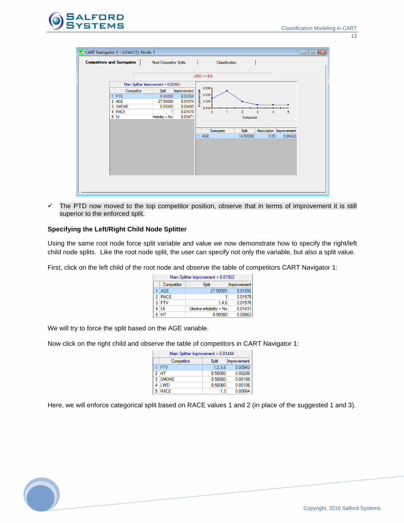
✓ The PTD now moved to the top competitor position, observe that in terms of improvement it is still superior to the enforced split.
Specifying the Left/Right Child Node Splitter
Using the same root node force split variable and value we now demonstrate how to specify the right/left
child node splits. Like the root node split, the user can specify not only the variable, but also a split value.
First, click on the left child of the root node and observe the table of competitors CART Navigator 1:
We will try to force the split based on the AGE variable.
Now click on the right child and observe the table of competitors in CART Navigator 1:
Here, we will enforce categorical split based on RACE values 1 and 2 (in place of the suggested 1 and 3).
Classification Modeling in CART
14
Copyright, 2016 Salford Systems
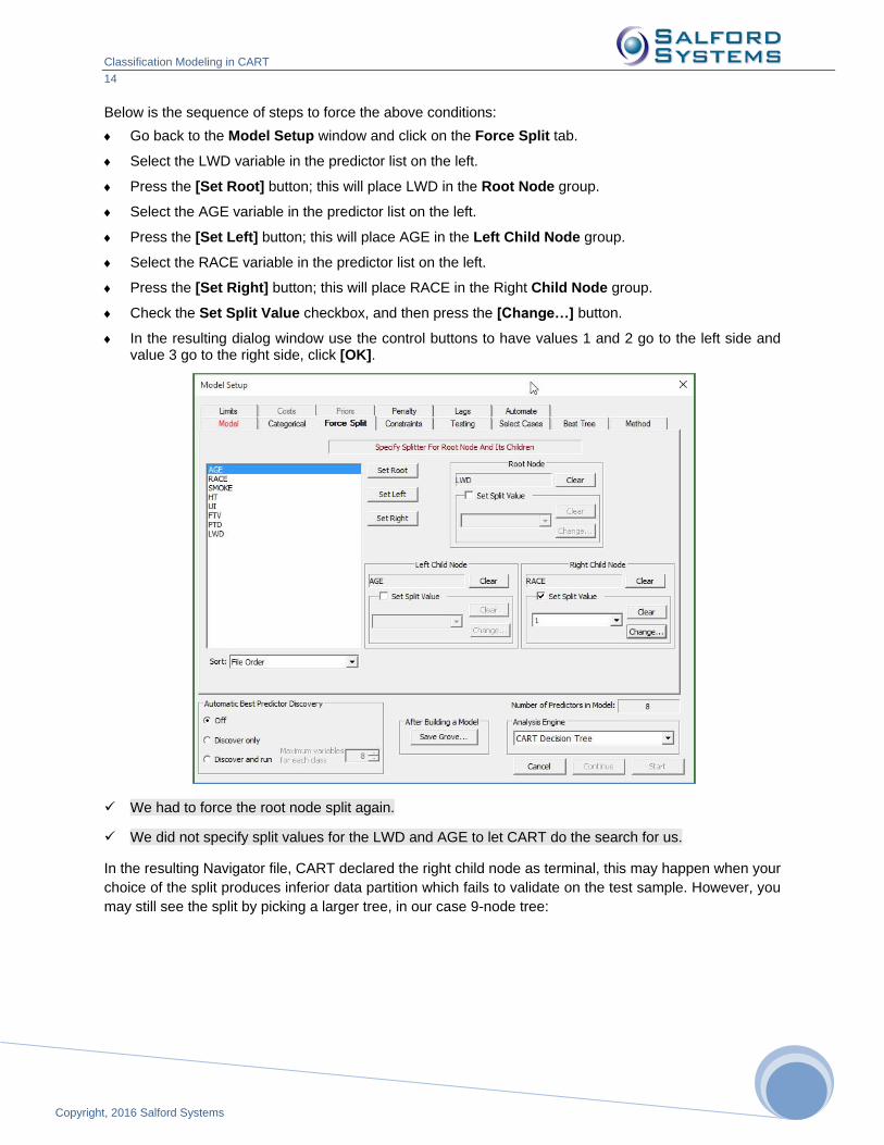
Below is the sequence of steps to force the above conditions:
Go back to the Model Setup window and click on the Force Split tab.
Select the LWD variable in the predictor list on the left.
Press the [Set Root] button; this will place LWD in the Root Node group.
Select the AGE variable in the predictor list on the left.
Press the [Set Left] button; this will place AGE in the Left Child Node group.
Select the RACE variable in the predictor list on the left.
Press the [Set Right] button; this will place RACE in the Right Child Node group.
Check the Set Split Value checkbox, and then press the [Change…] button.
In the resulting dialog window use the control buttons to have values 1 and 2 go to the left side and value 3 go to the right side, click [OK].
✓ We had to force the root node split again.
✓ We did not specify split values for the LWD and AGE to let CART do the search for us.
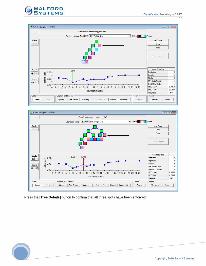
In the resulting Navigator file, CART declared the right child node as terminal, this may happen when your
choice of the split produces inferior data partition which fails to validate on the test sample. However, you
may still see the split by picking a larger tree, in our case 9-node tree:
Classification Modeling in CART
15
Copyright, 2016 Salford Systems
151
5
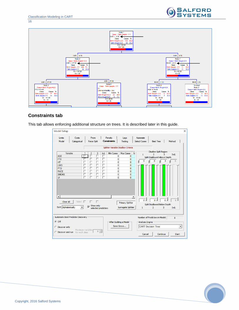
Press the [Tree Details] button to confirm that all three splits have been enforced:
Classification Modeling in CART
16
Copyright, 2016 Salford Systems
Constraints tab
This tab allows enforcing additional structure on trees. It is described later in this guide.

Classification Modeling in CART
17
Copyright, 2016 Salford Systems
171
7
Testing tab PARTITION
This generic tab offers a number of options to partition your data into learn, test, and validate samples. It
also includes cross-validation as an alternative. The tab is described in detail in the SPM Infrastructure
guide.
There are a number of different test method available. They include the include the following. These
test methods are described in detail in the SPM Infrastructure guide.
No independent testing – Results in an exploratory model with no independent testing. Resubstitution is used instead to approximate a test sample.
Fraction of cases selected at random. Specifies a fraction of cases selected at random for testing and, optionally, validation.
Test sample contained in a separate file. The test sample is contained in a separate dataset.
Cross Validation—v-fold cross validation. Request number of folds, for example, 2 or 5 or 20
Cross Validation—Variable determines CV bins. Specify variable which assigns records to cross-validation bins.
Variable seperates learn, test, (holdout). Specify variable which separates learn and test samples.
Classification Modeling in CART
18
Copyright, 2016 Salford Systems
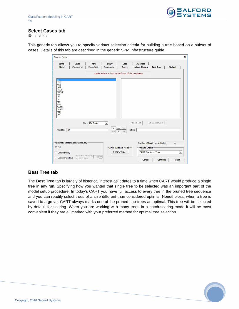
Select Cases tab SELECT
This generic tab allows you to specify various selection criteria for building a tree based on a subset of
cases. Details of this tab are described in the generic SPM Infrastructure guide.
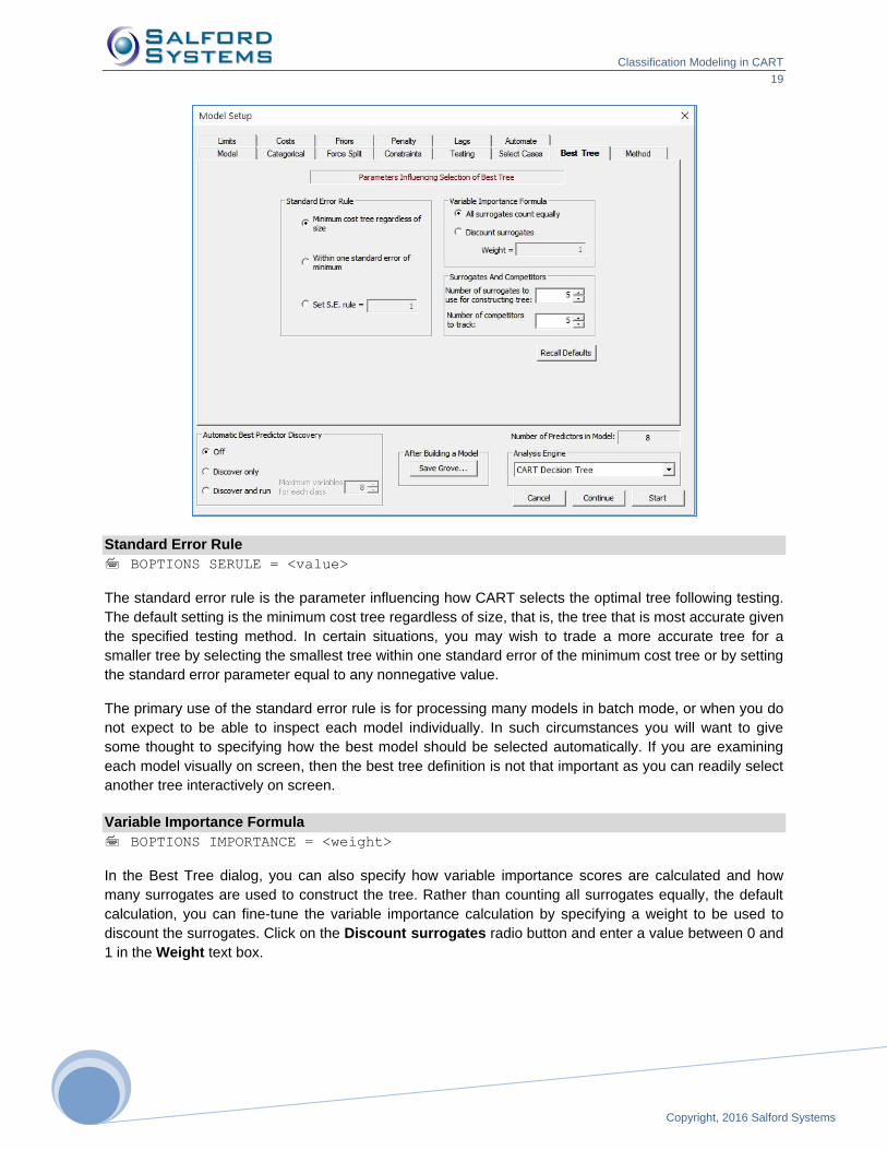
Best Tree tab
The Best Tree tab is largely of historical interest as it dates to a time when CART would produce a single
tree in any run. Specifying how you wanted that single tree to be selected was an important part of the
model setup procedure. In today’s CART you have full access to every tree in the pruned tree sequence
and you can readily select trees of a size different than considered optimal. Nonetheless, when a tree is
saved to a grove, CART always marks one of the pruned sub-trees as optimal. This tree will be selected
by default for scoring. When you are working with many trees in a batch-scoring mode it will be most
convenient if they are all marked with your preferred method for optimal tree selection.
Classification Modeling in CART
19
Copyright, 2016 Salford Systems
191
9
Standard Error Rule
BOPTIONS SERULE = <value>
The standard error rule is the parameter influencing how CART selects the optimal tree following testing.
The default setting is the minimum cost tree regardless of size, that is, the tree that is most accurate given
the specified testing method. In certain situations, you may wish to trade a more accurate tree for a
smaller tree by selecting the smallest tree within one standard error of the minimum cost tree or by setting
the standard error parameter equal to any nonnegative value.
The primary use of the standard error rule is for processing many models in batch mode, or when you do
not expect to be able to inspect each model individually. In such circumstances you will want to give
some thought to specifying how the best model should be selected automatically. If you are examining
each model visually on screen, then the best tree definition is not that important as you can readily select
another tree interactively on screen.
Variable Importance Formula
BOPTIONS IMPORTANCE = <weight>
In the Best Tree dialog, you can also specify how variable importance scores are calculated and how
many surrogates are used to construct the tree. Rather than counting all surrogates equally, the default
calculation, you can fine-tune the variable importance calculation by specifying a weight to be used to
discount the surrogates. Click on the Discount surrogates radio button and enter a value between 0 and
1 in the Weight text box.

Classification Modeling in CART
20
Copyright, 2016 Salford Systems
Number of Surrogates
BOPTIONS SURROGATES = <n>
After CART has found the best splitter (primary splitter) for any node it proceeds to look for surrogate
splitters: splitters that are similar to the primary splitter and can be used when the primary split variable is
missing. You have control over the number of surrogates CART will search for; the default value is five.
When there are many predictors with similar missing value patterns you might want to increase the
default value.
You can increase or decrease the number of surrogates that CART searches for and saves by entering a value in the Number of surrogates to use for constructing tree box.
✓ The number of surrogates that can be found will depend on the specific circumstances of each node. In some cases there are no surrogates at all. Your specification sets limits on how many will be searched for but does not guarantee that this is the number that will actually be found.
✓ If all surrogates at a given node are missing or no surrogates were found for that particular node, a case that has a missing value for the primary splitter will be moved to the left or right child node according to a default rule discussed later.
✓ Because the number of surrogates you request can affect the details of the tree grown we have placed this control on the Best Tree tab. Usually the impact of this setting on a tree will be small, and it will only affect trees grown on data with missing values.
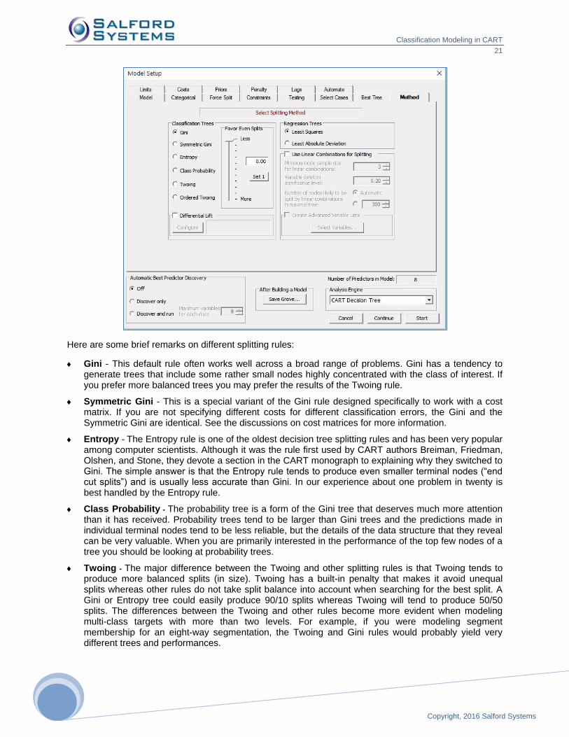
Method Tab
The Method tab allows you to specify the splitting rule used to construct the classification or regression
tree and to turn on the linear combinations option.
Splitting Rules
METHOD [ GINI | SYMGINI | TWOING | ORDERED | PROB | ENTROPY ]
A splitting rule is a method and strategy for growing a tree. A good splitting rule is one that yields accurate
trees! Since we often do not know which rule is best for a specific problem it is a good practice to
experiment. For classification trees the default rule is the Gini. This rule was introduced in the CART
monograph and was selected as the default because it generally works quite well. We have to agree with
the original CART authors: working with many hundreds of data sets in widely different subject matters we
have still seen the Gini rule to be an excellent choice. Further, there is often only a small difference in
performance among the rules.
However, there will be circumstances in which the performance between, say, the Gini and Entropy is
quite substantial, and we have worked on problems where using the Twoing rule has been the only way
to obtain satisfactory results. Accuracy is not the only consideration people weigh when deciding on
which model to use. Simplicity and comprehensibility can also be important. While the Gini might give you
the most accurate tree, the Twoing rule might tell a more persuasive story or yield a smaller although
slightly less accurate tree. Our advice is to not be shy about trying out the different rules and settings
available on the Method tab.
Classification Modeling in CART
21
Copyright, 2016 Salford Systems
212
1
Here are some brief remarks on different splitting rules:
Gini - This default rule often works well across a broad range of problems. Gini has a tendency to generate trees that include some rather small nodes highly concentrated with the class of interest. If you prefer more balanced trees you may prefer the results of the Twoing rule.
Symmetric Gini - This is a special variant of the Gini rule designed specifically to work with a cost matrix. If you are not specifying different costs for different classification errors, the Gini and the Symmetric Gini are identical. See the discussions on cost matrices for more information.
Entropy - The Entropy rule is one of the oldest decision tree splitting rules and has been very popular among computer scientists. Although it was the rule first used by CART authors Breiman, Friedman, Olshen, and Stone, they devote a section in the CART monograph to explaining why they switched to Gini. The simple answer is that the Entropy rule tends to produce even smaller terminal nodes (“end cut splits”) and is usually less accurate than Gini. In our experience about one problem in twenty is best handled by the Entropy rule.
Class Probability - The probability tree is a form of the Gini tree that deserves much more attention than it has received. Probability trees tend to be larger than Gini trees and the predictions made in individual terminal nodes tend to be less reliable, but the details of the data structure that they reveal can be very valuable. When you are primarily interested in the performance of the top few nodes of a tree you should be looking at probability trees.
Twoing - The major difference between the Twoing and other splitting rules is that Twoing tends to produce more balanced splits (in size). Twoing has a built-in penalty that makes it avoid unequal splits whereas other rules do not take split balance into account when searching for the best split. A Gini or Entropy tree could easily produce 90/10 splits whereas Twoing will tend to produce 50/50 splits. The differences between the Twoing and other rules become more evident when modeling multi-class targets with more than two levels. For example, if you were modeling segment membership for an eight-way segmentation, the Twoing and Gini rules would probably yield very different trees and performances.

Classification Modeling in CART
22
Copyright, 2016 Salford Systems
Ordered Twoing - The Ordered Twoing rule is useful when your target levels are ordered classes. For example, you might have customer satisfaction scores ranging from 1 to 5 and in your analysis you want to think of each score as a separate class rather than a simple score to be predicted by a regression. If you were to use the Gini rule CART would think of the numbers 1,2,3,4, and 5 as arbitrary labels without having any numeric significance. When you request Ordered Twoing you are telling CART that a “4” is more similar to a “5” than it is to a “1.” You can think of Ordered Twoing as developing a model that is somewhere between a classification and a regression.
✓ Ordered Twoing works by making splits that tend to keep the different levels of the target together in a natural way. Thus, we would favor a split that put the “1” and “2” levels together on one side of the tree and we would want to avoid splits that placed the “1” and “5” levels together. Remember that the other splitting rules would not care at all which levels were grouped together because they ignore the numeric significance of the class label.
As always, you can never be sure which method will work best. We have seen naturally ordered targets
that were better modeled with the Gini method. You will need to experiment.
✓ Ordered Twoing works best with targets with numeric levels. When a target is a character variable, the ordering conducted by CART might not be to your liking. See the command reference manual section on the DISCRETE command for more useful information.
Favor Even Splits
METHOD POWER=<x>
The “favor even splits” control is also on the Method tab and offers an important way to modify the action
of the splitting rules. By default, the setting is 0, which indicates no bias in favor of even or uneven splits.
In the display below we have set the splitting rule to Twoing and the “favor even splits” setting to 1.00.
The GUI limits your POWER setting to a maximum value of 2.00. This is to protect users from setting
outlandish values. There are situations, however, in which a higher setting might be useful, and if so you
will need to enter a command with a POWER setting of your choice. Using values greater than 5.00 is
probably not helpful.
✓ On binary targets when both “Favor Even Splits” and the unit cost matrix are set to 0, Gini, Symmetric Gini, Twoing, and Ordered Twoing will produce near identical results.
Although we make recommendations below as to which splitting rule is best suited to which type of
problem, it is good practice to always use several splitting rules and compare the results. You should
experiment with several different splitting rules and should expect different results from each. As you work
with different types of data and problems, you will begin to learn which splitting rules typically work best
for specific problem types. Nevertheless, you should never rely on a single rule alone; experimentation is
always wise.

Classification Modeling in CART
23
Copyright, 2016 Salford Systems
232
3
The following rules of thumb are based on our experience in the telecommunications, banking, and
market research arenas, and may not apply to other subject areas. Nevertheless, they represent such a
consistent set of empirical findings that we expect them to continue to hold in other domains and data
sets more often than not.
For a two-level dependent variable that can be predicted with a relative error of less than 0.50, the Gini splitting rule is typically best.
For a two-level dependent variable that can be predicted with a relative error of only 0.80 or higher, Power-Modified Twoing tends to perform best.
For target variables with four to nine levels, Twoing has a good chance of being the best splitting rule.
For higher-level categorical dependent variables with 10 or more levels, either Twoing or Power-Modified Twoing is often considerably more accurate than Gini.
Linear Combination Splits
LINEAR N=<min_cases>, DELETE=<signif_level>, SPLITS=<max_splits>
To deal more effectively with linear structure, CART has an option that allows node splits to be made on
linear combinations of non-categorical variables. This option is implemented by clicking on the Use
Linear Combinations for Splitting check box on the Method tab as seen below.
The Minimum node sample size for linear combinations, which can be changed from the default of
three by clicking the up or down arrows, specifies the minimum number of cases required in a node for
linear combination splits to be considered. Nodes smaller than the specified size will be split on single
variables only.
✓ The default value is far too small for most practical applications. We would recommend using values such as 20, 50, 100 or more.
The Variable deletion significance level, set by default at 0.20, governs the backwards deletion of
variables in the linear combination stepwise algorithm. Using a larger setting will typically select linear
combinations involving fewer variables. We often raise this threshold to 0.40 for this purpose.
By default, CART automatically estimates the maximum number of linear combination splits in the
maximal tree. The automatic estimate may be overridden to allocate more linear combination workspace.
To do so, click on the Number of nodes likely to be split by linear combinations in maximal tree
radio button and enter a positive value.
✓ CART will terminate the model-building process prematurely if it finds that it needs more linear combination splits than were actually reserved.
✓ Linear combination splits will be automatically turned off for all nodes that have any constant predictors (all values the same for all records). Thus, having a constant predictor in the training data will effectively turn off linear combinations for the entire tree.

Classification Modeling in CART
24
Copyright, 2016 Salford Systems
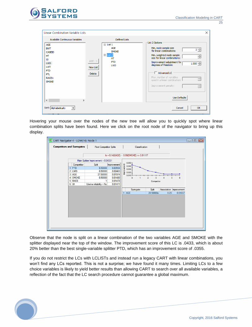
LC Lists: Create Advanced Variable Lists
LCLIST <variable>, <variable>, …
LC lists are a new addition to CART and can radically improve the predictive power and intuitive
usefulness of your trees. In legacy CART if you request a search for linear combination splitters ALL the
numeric variables in your predictor (KEEP) list are eligible to enter the linear combination (LC). In every
node with a large enough sample size CART will look for the best possible LC regardless of which
variables combine to produce that LC.
We have found it helpful to impose some structure on this process by allowing you to organize variables
into groups from which LCs can be constructed. If you create such groups, then any LC must be
constructed entirely from variables found in a single group. In a biomedical study you might consider
grouping variables into demographics such as AGE and RACE, lifestyle or behavioral variables such as
SMOKE and FTV, and medical history and medical condition variables such as UI, PTD, and LWT.
Specifying LCLISTS in this way will limit any LCs constructed to those that can be created from the
variables in a single list.
✓ Time series analysts can create one LCLIST for each predictor and its lagged values. LCs constructed from such a list can be thought of as distributed lag predictors.
✓ A variable can appear on more than one LCLIST, meaning that LC lists can overlap. You can even create an LCLIST with all numeric variables on it if you wish.
Below we have checked the box that activates LC lists for our example:
Press the [Select Variables] button to bring up a window in which you may create your LC Advanced Variables lists.
✓ Only numeric variables will be displayed in this window. Categorical variables will not be considered for incorporation into an LC even if they are simple 0/1 indicators. This is one good reason to treat your 0/1 indicators as numeric rather than categorical predictors.
Press the [New List] button to get started and then select the variables you want to include in the first list.
We will select AGE and SMOKE. Add them and then click again on New List to start a second list. Now
Add HT, PTD, LWD and click OK to complete the LCLIST setup. Click Start to begin the run.
Classification Modeling in CART
25
Copyright, 2016 Salford Systems
252
5
Hovering your mouse over the nodes of the new tree will allow you to quickly spot where linear
combination splits have been found. Here we click on the root node of the navigator to bring up this
display.
Observe that the node is split on a linear combination of the two variables AGE and SMOKE with the
splitter displayed near the top of the window. The improvement score of this LC is .0433, which is about
20% better than the best single-variable splitter PTD, which has an improvement score of .0355.
If you do not restrict the LCs with LCLISTs and instead run a legacy CART with linear combinations, you
won’t find any LCs reported. This is not a surprise; we have found it many times. Limiting LCs to a few
choice variables is likely to yield better results than allowing CART to search over all available variables, a
reflection of the fact that the LC search procedure cannot guarantee a global maximum.

Classification Modeling in CART
26
Copyright, 2016 Salford Systems
Limits Tab
The Limits tab allows you to specify additional tree-building control options and settings. You should not
hesitate to learn the meaning and use of these controls, as they can be the key to getting the best results.
Parent Node Minimum Cases (Do Not Split Node if Sample Less Than)
LIMIT ATOM = <N>
When do we admit that we do not have enough data to continue? Theoretically, we can continue splitting
nodes until we run out of data, for example, when there is only one record left in a node. In practice it
makes sense to stop tree growing when the sample size is so small that no one would take the split
results seriously. The default setting for the smallest node we consider splitting is 10, but we frequently
set the minimum to 20, 50, 100 or even 200 in very large samples.
Terminal Node Minimum Cases (Do Not Create Terminal Node Smaller Than)
LIMIT MINCHILD = <N>
This control specifies the smallest number of observations that may be separated into a child node. A
large node might theoretically be split by placing one record in one child node and all other records into
the other node. However, such a split would be rightfully regarded as unsatisfactory in most instances.
The MINCHILD control allows you to specify a smallest child node, below which no nodes can be
constructed. Naturally, if you set the value too high you will prevent the construction of any useful tree.
✓ Increasing allowable parent and child node sizes enables you to both control tree growth and to potentially fit larger problems into limited workspace (RAM).
✓ You will certainly want to override the default settings when dealing with large datasets.

Classification Modeling in CART
27
Copyright, 2016 Salford Systems
272
7
✓ The parent node limit (ATOM) must be at least twice the terminal node (MINCHILD) limit and otherwise will be adjusted by CART to comply with the parent limit setting.
✓ We recommend that ATOM be set to at least three times MINCHILD to allow CART to consider a reasonable number of alternative splitters near the bottom of the tree. If ATOM is only twice MINCHILD then a node that is just barely large enough to be split can be split only into two equal-sized children.
Minimum Complexity
BOPTIONS COMPLEXITY = <x> [,SCALED]
This is a truly advanced setting with no good short explanation for what it means, but you can quickly
learn how to use it to best limit the growth of potentially large trees. The default setting of zero allows the
tree-growing process to proceed until the “bitter end”. Setting complexity to a value greater than zero
places a penalty on larger trees, and causes CART to stop its tree-growing process before reaching the
largest possible tree size. When CART reaches a tree size with a complexity parameter equal to or
smaller than your pre-specified value, it stops the tree-splitting process on that branch. If the complexity
parameter is judiciously selected, you can save computer time and fit larger problems into your available
workspace. (See the main reference manual for guidance on selecting a suitable complexity parameter.)
✓ Check the Complexity Parameter column in the TREE SEQUENCE section of the Classic Output to get the initial feel for which complexity values are applicable for your problem.
The Scale Regression check box specifies that, for a regression problem, the complexity parameter
should be scaled up by the learn-sample size.
Dataset Size Warning Limit for Cross-Validation
BOPTIONS CVLEARN = <N>
By default, 3,000 is the maximum number of cases allowed in the learning sample before cross validation
is disallowed and a test sample is required. To use cross validation on a file containing more than 3,000
records, increase the value in this box to at least the number of records in your data file.
Maximum number of nodes
LIMIT NODES = <N>
Allows you to specify a maximum allowable number of nodes in the largest tree grown. If you do not
specify a limit CART may allow as many as one terminal node per data record. When a limit on NODES is
specified the tree generation process will stop when the maximum allowable number of nodes (internal
plus terminal) is reached. This is a crude but effective way to limit tree size.
Depth
LIMIT DEPTH = <N>
This setting limits the tree growing to a maximum depth. The root node corresponds to the depth of one.
Limiting a tree in this way is likely to yield an almost perfectly balanced tree with every branch reaching
the same depth. While this may appeal to your aesthetic sensibility it is unlikely to be the best tree for
predictive purposes.
By default CART sets the maximum DEPTH value so large that it will never be reached.

Classification Modeling in CART
28
Copyright, 2016 Salford Systems
✓ Unlike complexity, these NODES and DEPTH controls may handicap the tree and result in inferior performance.
✓ Some decision tree vendors set depth values to small limits such as five or eight. These limits are generally set very low to create the illusion of fast data processing. If you want to be sure to get the best tree you need to allow for somewhat deeper trees.
Learn Sample Size (LEARN)
LIMIT LEARN = <N>
The LEARN setting limits CART to processing only the first part of the data available and simply ignoring
any data that comes after the allowed records. This is useful when you have very large files and want to
explore models based on a small portion of the initial data. The control allows for faster processing of the
data because the entire data file is never read.
Test Sample Size
LIMIT TEST = <N>
The TEST setting is similar to LEARN: it limits the test sample to no more than the specified number of
records for testing. The test records are taken on a first-come-first served basis from the beginning of the
file. Once the TEST limit is reached no additional test data are processed.
Random Subsample Nodes Exceeding
LIMIT SUBSAMPLE = <N>
Node sub-sampling is an interesting approach to handling very large data sets and also serves as a
vehicle for exploring model sensitivity to sampling variation. Although node sub-sampling was introduced
in the first release of the CART mainframe software in 1987, we have not found any discussion of the
topic in the scientific literature. We offer a brief discussion here.
Node sub-sampling is a special form of sampling that is triggered for special purposes during the
construction of the tree. In node sub-sampling the analysis data are not sampled. Instead we work with
the complete analysis data set. When node sub-sampling is turned on we conduct the process of
searching for a best splitter for a node on a subsample of the data in the node. For example, suppose our
analysis data set contained 100,000 records and our node sub-sampling parameter was set to 5,000. In
the root node we would take our 100,000 records and extract a random sample of 5,000. The search for
the best splitter would be conducted on the 5,000 random record extract. Once found, the splitter would
be applied to the full analysis data set. Suppose this splitter divided the 100,000 root node into 55,000
records on the left and 45,000 records on the right. We would then repeat the process of selecting 5,000
records at random in each of these child nodes to find their best splitters.
As you can see, the tree generation process continues to work with the complete data set in all respects
except for the split search procedure. By electing to use node sub-sampling we create a shortcut for split
finding that can materially speed up the tree-growing process.
But is node sub-sampling a good idea? That will depend in part on how rare the target class of interest is.
If the 100,000 record data set contains only 1,000 YES records and 99,000 NO records, then any form of
sub-sampling is probably not helpful. In a more balanced data set the cost of an abbreviated split search
might be minimal and it is even possible that the final tree will perform better. Since we cannot tell without
trial and error we would recommend that you explore the impact of node sub-sampling if you are inclined
to consider this approach.

Classification Modeling in CART
29
Copyright, 2016 Salford Systems
292
9
Model Missing Values
On request, CART will automatically add missing value indicator variables (MVIs) to your list of predictors
and conduct a variety of analyses using them. For a variable named X1, the MVI will be named X1_MIS
and coded as 1 for every row with a missing value for X1 and 0 otherwise. If you activate this control, the
MVIs will be created automatically (as temporary variables) and will be used in the CART tree if they have
sufficient predictive power. MVIs allow formal testing of the core predictive value of knowing that a field is
missing.
Create missing indicator variables
BOPTIONS MISSING=<YES|NO|DISCRETE|CONTINUOUS|LIST=varlist>
There are four different strategies to create missing value indicators (MVIs):
None – do not create MVIs.
All variables – create MVIs for all variables that have missing values.
Categorical only – create MVIs for categorical variables only.
Continuous only – create MVIs for continuous variables only.
✓ The command line offers additional option to create MVIs for a specific subset of variables.
Create "missing" categorical level
DISCRETE MISSING = [ MISSING | ALL | LEGAL | TARGET ]
For categorical variables an MVI can be accommodated in two ways: by adding a separate MVI variable
as show above, or by treating missing as a valid "level."
The following options are available:
None – do not create a new “missing” category.
All variables – create a new missing category in categorical predictors and the target (if applicable).
Predictors only – create a new missing category in categorical predictors only.
Target only – create a new missing category in the target (if applicable).
Costs Tab MISCLASS COST=<value> CLASSIFY <origin_class> AS <predicted>
Because not all mistakes are equally serious or equally costly, decision makers are constantly weighing
quite different costs. If a direct mail marketer sends a flyer to a person who is uninterested in the offer the
marketer may waste $1.00. If the same marketer fails to mail to a would-be customer, the loss due to the
foregone sale might be $50.00. A false positive on a medical test might cause additional more costly tests
amounting to several hundreds of dollars. A false negative might allow a potentially life-threatening illness
to go untreated. In data mining, costs can be handled in two ways:
Post-analysis basis where costs are considered after a cost-agnostic model has been built.
During-analysis basis in which costs are allowed to influence the details of the model.
CART is unique in allowing you to incorporate costs into your analysis and decision making using either
of these two strategies.
To incorporate costs of mistakes directly into your CART tree, complete the matrix in the Costs tab
illustrated below. For example, if misclassifying low birth weight babies (LOW=1) is more costly than

Classification Modeling in CART
30
Copyright, 2016 Salford Systems
misclassifying babies who are not low birth weight (LOW=0), you may want to assign a penalty of two to
misclassifying class 1 as 0.
✓ Only cell ratios matter, that is, the actual value in each cell of the cost matrix is of no consequence—setting costs to 1 and 2 for the binary case is equivalent to setting costs to 10 and 20.
✓ In a two-class problem, set the lower cost to 1.00 and then set the higher cost as needed. You may find that a small change in a cost is all that is needed to obtain the balance of correct and incorrect and the classifications you are looking for. Even if one cost is 50 times greater than another, using a setting like 2 or 3 may be adequate.
✓ On binary classification problems, manipulating costs is equivalent to manipulating priors and vice versa. On multilevel problems, however, costs provide more detailed control over various misclassifications than do priors.
✓ By default, all costs are set to one (unit costs).
To change costs anywhere in the matrix, click on the cell you wish to alter and enter a positive numeric
value in the text box called Cost. To specify a symmetrical cost matrix, enter the costs in the upper right
triangle of the cost matrix and press the [Symmetrical] button. CART automatically updates the
remaining cells with symmetrical costs. Press the [Defaults] button to restore to the unit costs.
✓ CART requires all costs to be strictly positive (zero is not allowed). Use small values, such as .001, to effectively impose zero costs in some cells.
✓ We recommend conducting your analyses with the default costs until you have acquired a good understanding of the data from a cost-neutral perspective.

Classification Modeling in CART
31
Copyright, 2016 Salford Systems
313
1
Priors tab PRIORS[ EQUAL | LEARN | TEST | DATA | MIX]
PRIORS SPECIFY <class1> = <value1>, …
The Priors tab is one of the most important options you can set in shaping a classification analysis and
you need to understand the basics to get the most out of CART. Although the PRIORS terminology is
unfamiliar to most analysts the core concepts are relatively easy to grasp. Market researchers and
biomedical analysts make use of the priors concepts routinely but in the context of a different vocabulary.
We start by discussing a straightforward 0/1 or YES/NO classification problem. In most real world
situations, the YES or 1 group is relatively rare. For example, in a large field of prospects only a few
become customers, relatively few borrowers default on their loans, only a tiny fraction of credit card
transactions and insurance claims are fraudulent, etc. The relative rarity of a class in the real world is
usually reflected in the data available for analysis. A file containing data on 100,000 borrowers might
include no more than 4,000 bankrupts for a mainstream lender.
Such unbalanced data sets are quite natural for CART and pose no special problems for analysis. This is
one of CART’s great strengths and differentiates CART from other analytical tools that do not perform well
unless the data are “balanced.”
The CART default method for dealing with unbalanced data is to conduct all analyses using measures
that are relative to each class. In our example of 100,000 records containing 4,000 bankrupts, we will
always work with ratios that are computed relative to 4,000 for the bankrupts and relative to 96,000 for the
non-bankrupts. By doing everything in relative terms we bypass completely the fact that one of the two
groups is 24 times the size of the other.
This method of bookkeeping is known as PRIORS EQUAL. It is the default method used for classification
trees and often works supremely well. It is the setting we almost always use to start our exploration of
new data. This default setting frequently gives the most satisfactory results because each class is treated
as equally important for the purpose of achieving classification accuracy.
Priors are usually specified as fractions that sum to 1.0. In a two-class problem EQUAL priors would be
expressed numerically as 0.50, 0.50, and in a three-class problem they would be expressed as 0.333,
0.333, 0.333.
✓ PRIORS may look like weights but they are not weights. Priors reflect the relative size of a class after CART has made its adjustments. Thus, PRIORS EQUAL assures that no matter how small a class may be relative to the other classes, it will be treated as if it were of equal size.
✓ PRIORS DATA (or PRIORS LEARN or PRIORS TEST) makes no adjustments for relative class sizes. Under this setting small classes will have less influence on the CART tree and may even be ignored if they interfere with CART’s ability to classify the larger classes accurately.
✓ PRIORS DATA is perfectly reasonable when the importance of classification accuracy is proportional to class size. Consider a model intended to predict which political party will be voted for with the alternatives of Conservative, Liberal, Fringe1 and Fringe2. If the fringe parties together are expected to represent about 5% of the vote, an analyst might do better with PRIORS DATA, allowing CART to focus on the two main parties for achieving classification accuracy.
Classification Modeling in CART
32
Copyright, 2016 Salford Systems
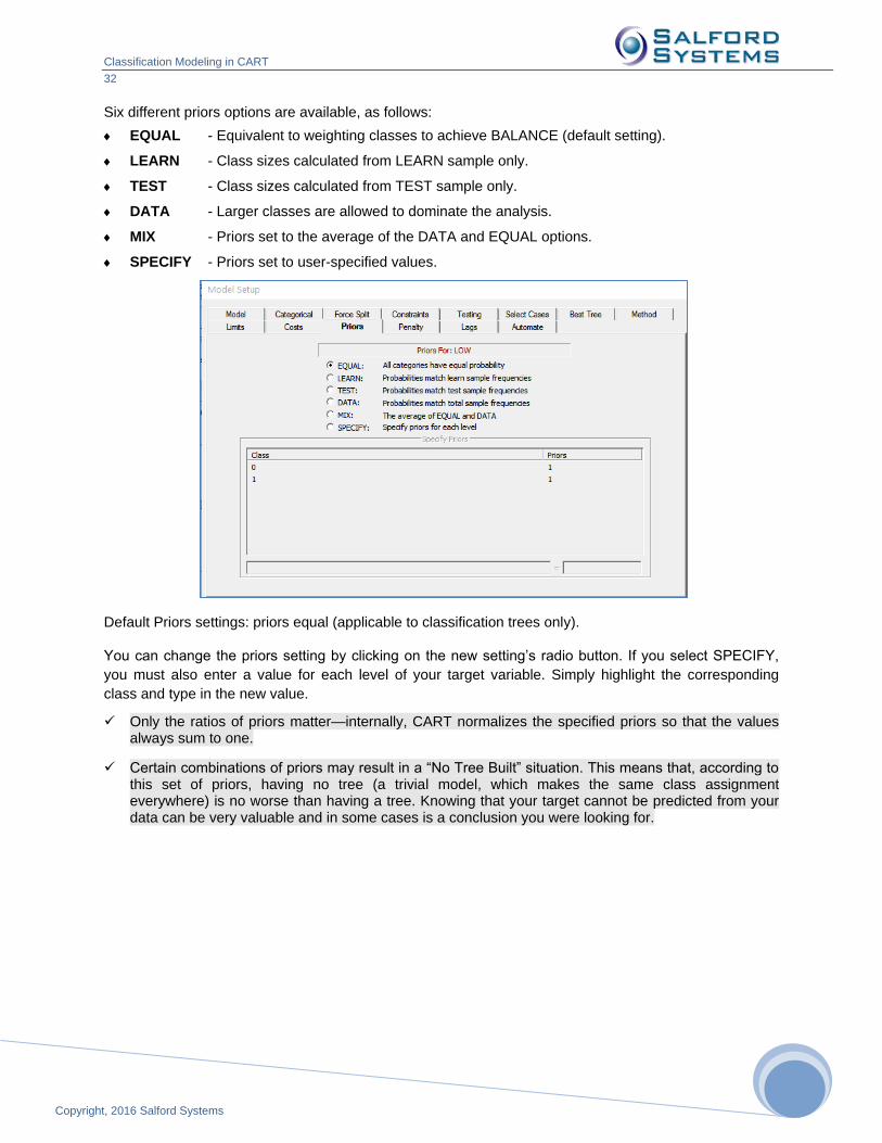
Six different priors options are available, as follows:
EQUAL - Equivalent to weighting classes to achieve BALANCE (default setting).
LEARN - Class sizes calculated from LEARN sample only.
TEST - Class sizes calculated from TEST sample only.
DATA - Larger classes are allowed to dominate the analysis.
MIX - Priors set to the average of the DATA and EQUAL options.
SPECIFY - Priors set to user-specified values.
Default Priors settings: priors equal (applicable to classification trees only).
You can change the priors setting by clicking on the new setting’s radio button. If you select SPECIFY,
you must also enter a value for each level of your target variable. Simply highlight the corresponding
class and type in the new value.
✓ Only the ratios of priors matter—internally, CART normalizes the specified priors so that the values always sum to one.
✓ Certain combinations of priors may result in a “No Tree Built” situation. This means that, according to this set of priors, having no tree (a trivial model, which makes the same class assignment everywhere) is no worse than having a tree. Knowing that your target cannot be predicted from your data can be very valuable and in some cases is a conclusion you were looking for.

Classification Modeling in CART
33
Copyright, 2016 Salford Systems
333
3
Penalty tab
The penalties available in the SPM were introduced by Salford Systems starting in 1997 and represent
important extensions to machine learning technology. Penalties can be imposed on variables to reflect a
reluctance to use a variable as a predictor. Of course, the modeler can always exclude a variable; the
penalty offers an opportunity to permit a variable into the model but only under special circumstances.
The three categories of penalty are:
Variable Specific Penalties: Each predictor can be assigned a custom penalty (light blue rectangle above).
PENALTY <var>=<penalty> [<var2> = <pen2>, <var3> = <pen3>, …]
Missing Value Penalty: Predictors are penalized to reflect how frequently they are missing. The penalty is recalculated for every node in the tree (purple rectangle above)
PENALTY /MISSING=1,1
High Level Categorical Penalty: Categorical predictors with many levels can distort a tree due to their explosive splitting power. The HLC penalty levels the playing field. (orange rectangle above)
HLC=<hlc_val1>,<hlc_val2>
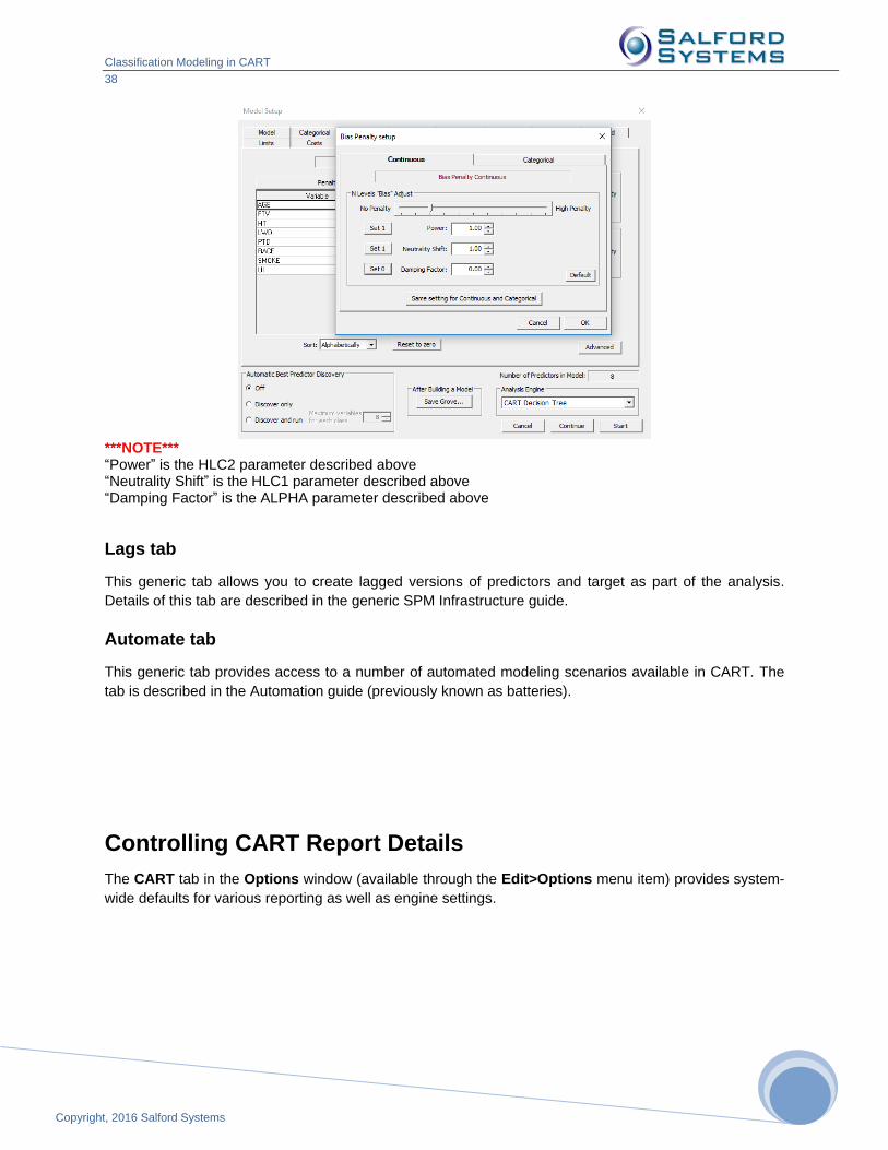
N Levels Bias Adjust: The essence of the possible "bias" in tree-based splitter selection is that predictors with a greater number of distinct values have an "advantage" in splitting. The bias adjustments correct for this bias (red rectangle above). PENALTY / CONTBIAS=<HLC1>,<HLC2>,<ALPHA>, CATBIAS=<HLC1>,<HLC2>,<ALPHA>

Classification Modeling in CART
34
Copyright, 2016 Salford Systems
A penalty will lower a predictor’s improvement score, thus making it less likely to be chosen as the
primary splitter. Penalties specific to particular predictors are entered in the left panel next to the predictor
name and may range from zero to one inclusive.
Penalties for missing values (for categorical and continuous predictors) and a high number of levels (for categorical predictors only) can range from "No Penalty" to "High Penalty" and are normally set via the slider on the Penalty tab, as seen in the following illustration.
In the screenshot above, we have set both the Missing Values and the HLC penalties to the frequently useful values of 1.00 (red rectangle and blue rectangle above, respectively).
Penalties on Variables
The penalty specified is the amount by which the variable’s improvement score is reduced before
deciding on the best splitter in a node. Imposing a 0.10 penalty on a variable will reduce its improvement
score by 10%. You can think of the penalty as a “handicap”: a 0.10 penalty means that the penalized
variable must be at least 10% better than any other variable to qualify as the splitter.
✓ Penalties may be placed to reflect how costly it is to acquire data. For example, in database and targeted marketing, selected data may be available only by purchase from specialized vendors. By penalizing such variables we make it more difficult for such variables to enter the tree, but they will enter when they are considerably better than any alternative predictor.
✓ Predictor-specific penalties have been used effectively in medical diagnosis and triage models. Predictors that are “expensive” because they require costly diagnostics, such as CT scans, or that can only be obtained after a long wait (say 48 hours for the lab results), or that involve procedures that are unpleasant for the patient, can be penalized. If penalizing these variables leads to models that are only slightly less predictive, the penalties help physicians to optimize diagnostic procedures.
Setting the penalty to 1 is equivalent to effectively removing this predictor from the predictor list.

Classification Modeling in CART
35
Copyright, 2016 Salford Systems
353
5
Missing Values Penalty
In CART, at every node, every predictor competes to be the primary splitter. The predictor with the best
improvement score becomes one. Variables with no missing values have their improvement scores
computed using all the data in the node, while variables with missing values have their improvement
scores calculated using only the subset with complete data. Since it is easier to be a good splitter on a
small number of records, this tends to give an advantage to variables with missing values. To level the
playing field, variables can be penalized in proportion to the degree to which they are missing. The
proportion missing is calculated separately at each node in the tree. For example, a variable with good
data for only 30% of the records in a node would receive only 30% of its calculated improvement score. In
contrast, a variable with good data for 80% of the records in a node would receive 80% of its
improvement score. A more complex formula is available for finer control over the missing value penalty
using the Advanced version of the Penalty tab (click the button in the green rectangle above).
Suppose you want to penalize a variable with 70% missing data very heavily, while barely penalizing a
variable with only 10% missing data. The Advanced option (click the button in the green rectangle
above) lets you do this by setting a fractional power on the percent of good data. For example, using the
square root of the fraction of good data to calculate the improvement factor would give the first variable
(with 70% missing) a .55 factor and the second variable (with 10% missing) a .95 factor.
The expression used to scale improvement scores is:
The default settings of a = 1, b = 0 disable the penalty entirely; every variable receives a factor of 1.0.
Useful penalty settings set a = 1 with b = 1.00, or 0.50. The closer b gets to 0 the smaller the penalty. The
fraction of the improvement kept for a variable is illustrated in the following table, where "%good" = the
fraction of observations with non-missing data for the predictor.
%good b=.75 b=.50
-----------------------------
0.9 0.92402108 0.948683298
0.8 0.84589701 0.894427191
0.7 0.76528558 0.836660027
0.6 0.68173162 0.774596669
0.5 0.59460355 0.707106781
0.4 0.50297337 0.632455532
0.3 0.40536004 0.547722558
0.2 0.29906975 0.447213595
0.1 0.17782794 0.316227766
In the bottom row of this table, we see that if a variable is only good in 10% of the data, it receives 10% credit if b=1, 17.78% credit if b=.75, and 31.62% credit if b=.50. If b=0, the variable receives 100% credit because we would be ignoring its degree of missingness.
✓ In most analyses, we find that the overall predictive power of a tree is unaffected by the precise setting of the missing value penalty. However, without any missing value penalty you might find heavily
bng_not_missiproportionaS

Classification Modeling in CART
36
Copyright, 2016 Salford Systems
missing variables appearing high up in the tree. The missing value penalty thus helps generate trees that are more appealing to decision makers.
High-Level Categorical (HLC) Penalty
Categorical predictors present a special challenge to decision trees. Because a 32-level categorical
predictor can split a data set in over two billion ways, even a totally random variable has a high probability
of becoming the primary splitter in many nodes. Such spurious splits do not prevent TreeNet from
eventually detecting the true data structure in large datasets, but they make the process inefficient. First,
spurious splits add unwanted nodes to a tree, and because they promote the fragmentation of the data
into added nodes, the reduced sample size as we progress down the tree makes it harder to find the best
splits.
To protect against this possibility, the SPM offers a high-level categorical predictor penalty used to reduce
the measured splitting power. On the Basic Penalty dialog, this is controlled with a simple slider (this is
the default view that you see in the picture on the previous page).
The Advanced Penalty (click the button in the green rectangle above) dialog allows access to the full
penalty expression. The improvement factor is expressed as:
By default, c = 1 and d = 0; these values disable the penalty. We recommend that the categorical variable
penalty be set to (c = 1, d = 1), which ensures that a categorical predictor has no inherent advantage over
a continuous variable with unique values for every record.
The missing value and HLC penalties apply uniformly to all variables. You cannot set different HLC or missing value penalties to different variables. You choose one setting for each penalty and it applies to all variables.
✓ You can set variable-specific penalties, general missing value, and HLC penalties. Thus, if categorical variable Z is also sometimes missing all three penalties could apply to this variable at the same time.
1
1_
_log1,1min 2
d
categoriesN
sizenodecS

Classification Modeling in CART
37
Copyright, 2016 Salford Systems
373
7
N-Levels Bias Adjust
PENALTY / CONTBIAS=<HLC1>,<HLC2>,<ALPHA>, CATBIAS=<HLC1>,<HLC2>,<ALPHA>
The essence of the possible "bias" in tree-based splitter selection is that predictors with a greater number
of distinct values have an "advantage" in splitting. We discuss this topic at length in technical papers and
here just describe how our penalties function. A key ratio describing a potential predictor in the training
data is the ratio of number of observations to the number of distinct predictor values.
This ratio is expressed as
𝑅𝐴𝑇𝐼𝑂 =𝑙𝑜𝑔2(𝑁𝑂𝐵𝑆)
𝑙𝑜𝑔2(𝑁𝑉𝐴𝐿𝑈𝐸𝑆) for continuous predictors and
𝑅𝐴𝑇𝐼𝑂 =𝑙𝑜𝑔2(𝑁𝑂𝐵𝑆)
(𝐽−1) where J is the number of levels for categorical predictors
We determine how much we want to damp this ratio with the user set tuning parameter ALPHA in the
following expression: DRATIO = 1 + ALPHA*LN(RATIO) + (1-ALPHA)*ln(1 + ln(RATIO)) with the default
ALPHA=0.
Observe that RATIO is defined in terms of log base 2 while DRATIO uses a natural log. DRATIO allows
us to move between a log (moderate) and a log-log (heavy) damping of the ratio with our
recommendation to start with log-log. With DRATIO computed we create a "penalty" that follows the
pattern of our HLC penalty. First, the DRATIO may be raised to a power which we typically set to 1.0
although values ranging from .25 to 5.0 could be useful. We refer to this as the "power" parameter
(HLC2).
The final improvement adjustment expression is 𝑃𝑒𝑛𝑎𝑙𝑡𝑦 = 1 − 𝐻𝐿𝐶1 + 𝐻𝐿𝐶1 ∗ 𝑅𝐴𝑇𝐼𝑂𝐻𝐿𝐶2 where
HLC1 is a user set tuning parameter between 0 and 1. The "penalty" multiplies the improvement score of
any potential splitter. When its value is greater than 1.0 the "penalty" is actually a booster that favors
a predictor. Note: the penalty is used to adjust the split improvement:
Adjust Split Improvement = Split Improvement*Penalty
So if Penalty = 1 then the penalty has no effect; If Penalty < 1 then the variable is less likely to be used
because its adjusted split improvement is smaller than it otherwise would be without the penalty; If
Penalty > 1 then the variable is more likely to be used because its adjusted split improvement is larger
than it otherwise would be without the penalty.
Our "penalty" can be seen as a weighted average of 1 and DRATIO^HLC2 with weights (1-HLC1) and
HLC1. If HLC1 is set to 1.0 then we work only with the power modified DRATIO and clearly if HLC1=0 we
cancel any penalty. Values between 0 and 1 move the adjustment term towards 1 and thus diminish the
adjustment. The "penalty" can and probably should be tuned separately for continuous
and categorical variables. With three free parameters for each of continuous and categorical predictors,
the tuning of these adjustments can be complicated and we therefore recommend that modelers start with
the AUTOMATE BIASPENALTY to conduct a randomized search over plausible settings.
Bias Adjustment in the GUI
Classification Modeling in CART
38
Copyright, 2016 Salford Systems
***NOTE*** “Power” is the HLC2 parameter described above “Neutrality Shift” is the HLC1 parameter described above “Damping Factor” is the ALPHA parameter described above
Lags tab
This generic tab allows you to create lagged versions of predictors and target as part of the analysis.
Details of this tab are described in the generic SPM Infrastructure guide.
Automate tab
This generic tab provides access to a number of automated modeling scenarios available in CART. The
tab is described in the Automation guide (previously known as batteries).
Controlling CART Report Details
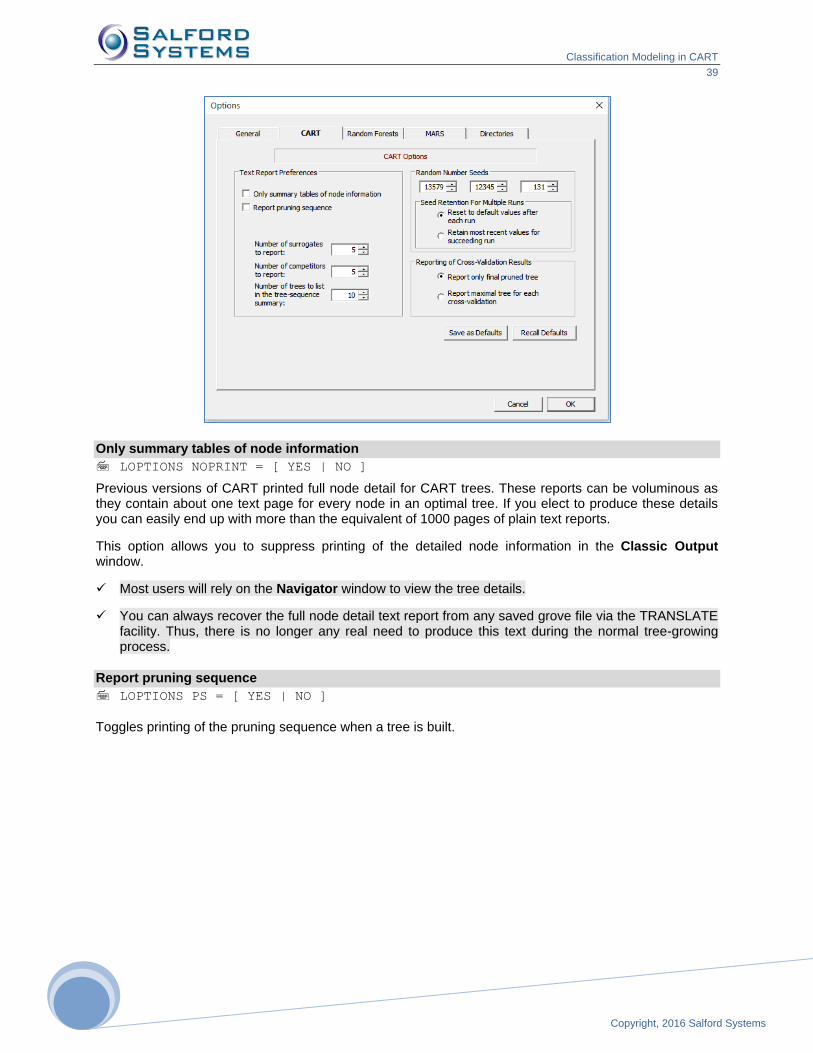
The CART tab in the Options window (available through the Edit>Options menu item) provides system-
wide defaults for various reporting as well as engine settings.
Classification Modeling in CART
39
Copyright, 2016 Salford Systems
393
9
Only summary tables of node information
LOPTIONS NOPRINT = [ YES | NO ]
Previous versions of CART printed full node detail for CART trees. These reports can be voluminous as they contain about one text page for every node in an optimal tree. If you elect to produce these details you can easily end up with more than the equivalent of 1000 pages of plain text reports.
This option allows you to suppress printing of the detailed node information in the Classic Output window.
✓ Most users will rely on the Navigator window to view the tree details.
✓ You can always recover the full node detail text report from any saved grove file via the TRANSLATE facility. Thus, there is no longer any real need to produce this text during the normal tree-growing process.
Report pruning sequence
LOPTIONS PS = [ YES | NO ]
Toggles printing of the pruning sequence when a tree is built.

Classification Modeling in CART
40
Copyright, 2016 Salford Systems
Number of Surrogates to Report
LOPTONS PRINT = <N>
This option sets the maximum number of surrogates that can appear in the text report and the navigator
displays.
✓ This setting only affects the displays in the text report and the Navigator windows. It does not affect the number of surrogates calculated.
✓ The maximum number of surrogates calculated is set in the Best Tree tab of the Model Setup dialog.
✓ You can elect to try to calculate 10 surrogate splitters for each node but then display only the top five. No matter how many surrogates you request you will get only as many as CART can find. In some nodes there are no surrogates found and the displays will be empty.
Number of Competitors to Report
LOPTIONS CPRINT = <N>
This option sets the maximum number of competitors that appear in reports.
✓ This option only affects CART’s classic output.
✓ Every variable specified in your KEEP list or checked off as an allowed predictor on your Model SetUp is a competitor splitter. Normally we do not want or need to see how every one of them performed. The default setting displays the top five but there is certainly no harm in setting this number to a much larger value.
✓ CART tests every allowed variable in its search for the best splitter. This means that CART always measures the splitting power of every predictor in every node. You only need to choose how much of this information you would like to be able to see in a navigator. Choosing a large number can increase the size of saved navigators/groves.
Number of Trees to List in the Tree Sequence Summary
BOPTIONS TREELIST = <N>
Each CART run prints a summary of the nested sequence of trees generated during growing and pruning.
The number of trees listed in the tree-sequence summary can be increased or decreased from the default
setting of 10 by entering a new value in the text box.
✓ This option only affects CART’s classic output.
Random-Number Seeds
SEED <N1>, <N2>, <N3>, [ NORETAIN | RETAIN ]
You can set the random-number seed and specify whether the seed is to remain in effect after a tree is
built or data are dropped down a tree. Normally the seed is reset to 13579, 12345, and 131 on start-up
and after each tree is constructed or after data are dropped down a tree. The seed will retain its latest
value after the tree is built if you click on the Retain most recent values for succeeding run radio
button.
Reporting of Cross-Validation Results
BOPTIONS { BRIEF | COPIOUS ]
If you use the cross-validation testing method, you can request a text report for each of the maximal trees
generated in each cross-validation run by clicking on the corresponding radio button for this option.

Classification Modeling in CART
41
Copyright, 2016 Salford Systems
414
1
For example, if testing is set to the default 10-fold cross validation, a report for each of the ten cross-
validated trees will follow the report on the final pruned tree in the text output. For this option to have full
effect be sure to uncheck the “Only summary tables of node information.” The GUI offers more a
convenient way to review these CV details.
Working with Navigators
The basics of working with navigators are described in detail in the CART Introduction guide. If you have
not already read that guide, we encourage you to do so. It contains important and pertinent information on
the use of CART result menus and dialogs.
In the next section we complete our exposition of the Navigator by explaining the remaining functions.
Viewing Auxiliary Variables Information
Here, we set up a new modeling run using GYMTUTOR.CSV dataset (available in the Sample Data
folder) with the following variable and tree type designations.
Target - SEGMENT
Predictors - TANNING, ANYPOOL, HOME, CLASSES
Categorical - SEGMENT, HOME, NFAMMEM
Auxiliary - HOME, CLASSES, FIT, NFAMMEM
Target Type - Classification/Logistic Binary
Press the [Start] button and look at the resulting Navigator window (we use color coding for
SEGMENT=2):
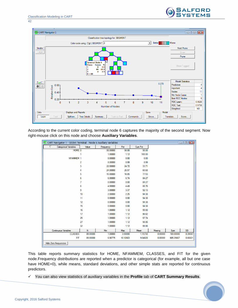
Classification Modeling in CART
42
Copyright, 2016 Salford Systems
According to the current color coding, terminal node 6 captures the majority of the second segment. Now
right-mouse click on this node and choose Auxiliary Variables.
This table reports summary statistics for HOME, NFAMMEM, CLASSES, and FIT for the given
node.Frequency distributions are reported when a predictor is categorical (for example, all but one case
have HOME=0), while means, standard deviations, and other simple stats are reported for continuous
predictors.
✓ You can also view statistics of auxiliary variables in the Profile tab of CART Summary Results.
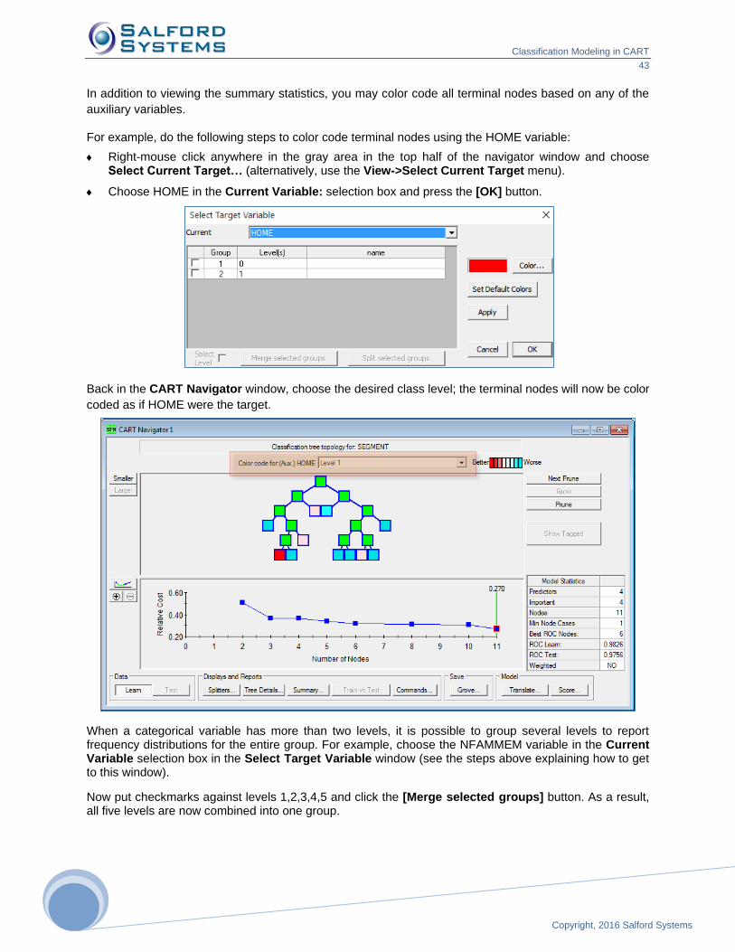
Classification Modeling in CART
43
Copyright, 2016 Salford Systems
434
3
In addition to viewing the summary statistics, you may color code all terminal nodes based on any of the
auxiliary variables.
For example, do the following steps to color code terminal nodes using the HOME variable:
Right-mouse click anywhere in the gray area in the top half of the navigator window and choose Select Current Target… (alternatively, use the View->Select Current Target menu).
Choose HOME in the Current Variable: selection box and press the [OK] button.
Back in the CART Navigator window, choose the desired class level; the terminal nodes will now be color
coded as if HOME were the target.
When a categorical variable has more than two levels, it is possible to group several levels to report frequency distributions for the entire group. For example, choose the NFAMMEM variable in the Current Variable selection box in the Select Target Variable window (see the steps above explaining how to get to this window).
Now put checkmarks against levels 1,2,3,4,5 and click the [Merge selected groups] button. As a result, all five levels are now combined into one group.
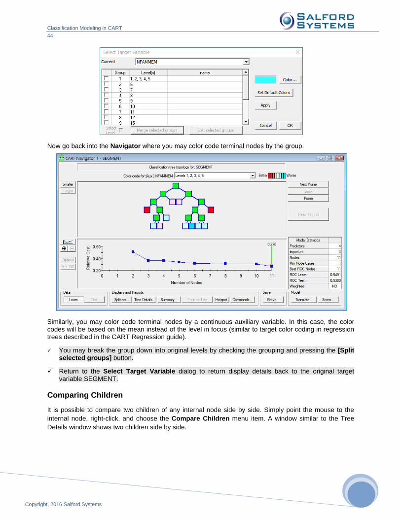
Classification Modeling in CART
44
Copyright, 2016 Salford Systems
Now go back into the Navigator where you may color code terminal nodes by the group.
Similarly, you may color code terminal nodes by a continuous auxiliary variable. In this case, the color codes will be based on the mean instead of the level in focus (similar to target color coding in regression trees described in the CART Regression guide).
✓ You may break the group down into original levels by checking the grouping and pressing the [Split selected groups] button.
✓ Return to the Select Target Variable dialog to return display details back to the original target variable SEGMENT.
Comparing Children
It is possible to compare two children of any internal node side by side. Simply point the mouse to the
internal node, right-click, and choose the Compare Children menu item. A window similar to the Tree
Details window shows two children side by side.
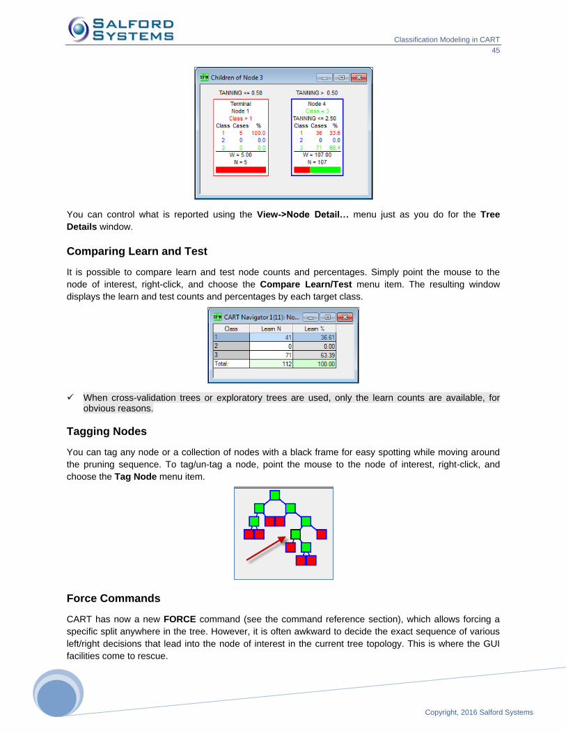
Classification Modeling in CART
45
Copyright, 2016 Salford Systems
454
5
You can control what is reported using the View->Node Detail… menu just as you do for the Tree
Details window.
Comparing Learn and Test
It is possible to compare learn and test node counts and percentages. Simply point the mouse to the
node of interest, right-click, and choose the Compare Learn/Test menu item. The resulting window
displays the learn and test counts and percentages by each target class.
✓ When cross-validation trees or exploratory trees are used, only the learn counts are available, for obvious reasons.
Tagging Nodes
You can tag any node or a collection of nodes with a black frame for easy spotting while moving around
the pruning sequence. To tag/un-tag a node, point the mouse to the node of interest, right-click, and
choose the Tag Node menu item.
Force Commands
CART has now a new FORCE command (see the command reference section), which allows forcing a
specific split anywhere in the tree. However, it is often awkward to decide the exact sequence of various
left/right decisions that lead into the node of interest in the current tree topology. This is where the GUI
facilities come to rescue.

Classification Modeling in CART
46
Copyright, 2016 Salford Systems
For example, to generate the FORCE command syntax that can be used to alter the splitting of the
internal node number 7 (the third node down on the right side branch of the tree in our example) simply
point to the node, right mouse click, then click Force Commands>Node Only menu item.
A new Notepad window opens up containing the FORCE command that imitates the splitting of the node
7 along with some comments:
Note that the RR sequence points to the node of interest (right child of the right child of the root node),
followed by the split variable and split value. You can change the splitter and/or the value, submit the
window and then rebuild CART tree to force a different split point.
If you click on the Force Commands>Node Plus Children menu item, the Notepad window will display
a collection of FORCE commands that reproduce the entire tree branch starting with the node of interest.
This way you may alter various splits and split values at different points in the branch and then build a
custom tree!
✓ Doing this with the root node, you have access to the entire tree topology and can easily construct a custom built tree.
Internally, CART uses surrogates to handle missing values at any split. The remaining two menu items in
the Force Commands pop-up menu are Node Only With Surrogates and Node Plus Children With
Surrogates. They generate not only the FORCE code for the main splitter, but also include all of the
surrogate splits. This will give you complete control over what happens at each individual split point. You
can modify it, submit the command window and then rebuild the tree to enforce the user-defined splits.
✓ The FORCE commands are cumulative, you may have as many of them as you like.

Classification Modeling in CART
47
Copyright, 2016 Salford Systems
474
7
✓ Empty FORCE command resets all of the previously accumulated FORCE commands.
Providing an inconsistent set of FORCE commands may stop your tree building prematurely.
CART was originally designed to remove the burden of split finding and also ensuring the best possible performance. By taking the control back into your hands, it is no longer guaranteed that the trees will be optimal and accurate. Use this facility at your own risk.
Displaying a Sub-tree
To display a portion of a tree originating from the internal node of interest, point the mouse to the node,
right-click, and choose the Display Tree menu item.
Saving and Opening Navigator Files
CART allows you to save the Navigator to a file and then later reload it. To save a Navigator file (also
known as the Grove), bring the Navigator window to the foreground and use the Save->Save Grove…
item from the File menu.
To open a Navigator file you have previously saved, use the Open->Open Grove… item from the File
menu.

Classification Modeling in CART
48
Copyright, 2016 Salford Systems
Opening a navigator in subsequent sessions allows you to continue your exploration of detailed and
summary reports for each of the trees in the nested sequence or to use the navigator for scoring or
translation.
All of these procedures are described in detail in the generic section of this manual.
Reopening the file does not reload the model setup specifications in the GUI dialogs. To do this, you should learn the basics of command-line use described in Command Line Control guide.
Printing Trees
To print the Main Tree (or a sub-tree), bring the tree window to the foreground (press the [Tree Details...]
button in the Navigator window) and then select Print… from the File menu (or use <Ctrl+P>). In the
Print dialog box, you can select the pages that will be printed and the number of copies, as well as
specify various printer properties. The Print dialog also displays a preview of the page layout; CART
automatically shifts the positions of the nodes so they are not split by page breaks.
To alter the tree layout prior to printing, press the [Page Setup…] button. As shown below, the current
layout is depicted in the tree preview window of the Page Setup dialog; as you change the settings, the
print-preview image changes accordingly. You can use the left and right arrows just below the sample
page image to change which page is previewed.

Classification Modeling in CART
49
Copyright, 2016 Salford Systems
494
9
The page setup options and their default settings are:
Node Gaps [0.10”]: Change the distance between the nodes by increasing or decreasing the horizontal setting and change the height of the tree branches by increasing or decreasing the vertical setting.
Orientation [portrait]: Choose portrait or landscape.
Tree Scale [100%]: Increase/decrease the overall size of the tree.
Border [thin]: Change the width of the page border or select “no border.”
Header: Enter text for header or select from the predefined settings by clicking on […]; predefined settings include file name, tree name, column #, row #, current date and time; also included here are the alignment options (left, right, center). (Note: To include an ampersand in the header, type two ampersands, &&.)
Footer: Replace default footer text (input file name, page row and column) by entering new text or select from the predefined settings by clicking on […]; predefined settings are similar to those for headers (see above).
Node Shapes: Change the non-terminal (node) and terminal node (term) default hexagon and rectangle shapes by clicking the down arrow and selecting an alternative shape.
Margins [0.50”]: Change left, right, top and bottom margins.

Classification Modeling in CART
50
Copyright, 2016 Salford Systems
Overlaying and Printing Gains Charts
You can overlay gains charts for nested trees in a CART sequence, for different CART analyses, and for
different classes of a target variable. To overlay two or more gains charts:
Select the corresponding navigator and select the tree of choice..
Click [Summary Reports…] and make sure the Gains Chart tab is active.
✓ Each click on the [Summary Reports…] button creates a new instance of the Summary Reports window. In this example we are overlaying the Class=1 models from two different sized trees.
Choose the right target class in the Tgt. Class selection box.
Repeat steps 1 through 3 as many times as needed to have all the gains charts you would like to overlay.
Select Gains Charts… from the View menu, which will open the Overlay Gains Charts dialog listing the charts you want to overlay in the right panel.
Click [Cum Lift], [Lift], [Gains], or [ROC] to request the corresponding overlay charts.

Classification Modeling in CART
51
Copyright, 2016 Salford Systems
515
1
Each chart is displayed in a unique color with a different plotting symbol, as seen in the illustration above.
To print the contents of the Overlay Gains Chart dialog box, select Print… from the File menu. To alter
the layout prior to printing, select Page Setup… from the File menu.
✓ The tables in the Gains Chart, Misclassification and Prediction Success dialog boxes can also be copied and pasted into spreadsheet and word processing programs such as Excel and Word.
All of these tables and graphs can also be exported into various graphical formats. They include *.bmp, *.emf, *.jpg, *.png, and *.wmf. To export, right-click on the table or graph and select Export… form the menu.

Classification Modeling in CART
52
Copyright, 2016 Salford Systems
Constraints and Structured Trees DISALLOW
In marketing applications we often think about predictors in terms of their role in influencing a consumer's
choice process. For example, we distinguish between characteristics of the consumer, over which the
marketer has no control, and characteristics of the product being offered, over which the marketer may
have some degree of control.
Normally CART will be unaware of the different strategic roles different variables may play within the
business context and a CART tree designed to predict response will mix variables of different roles as
needed to generate an accurate predictive model. However, it will often be useful to be able to
STRUCTURE a CART tree so that there is a systematic order in which the variables enter the tree.
For example, we may want the tree to use only characteristics of the consumer at the top of the tree and
to have only the bottom splits based on product characteristics. Such trees are very easy to read for their
strategy advice: first they segment a database into different types of consumer, and then they reveal the
product configurations or offers that best elicit response from each consumer segment.
CART now offers a powerful mechanism for generating structured trees by allowing you to specify where
a variable or group of variables are allowed to appear in the tree. The easiest way to structure a tree is to
group your predictor variables into lists and then to dictate the levels of the tree where each list is
permitted to operate. Thus, in our marketing example, we could specify that the consumer attributes list
can operate anywhere in the top four levels of the tree (but nowhere else) and that the product attributes
list can operate from level five and further down into the tree (but nowhere else). Structuring a tree in this
way will provide the marketer with exactly the type of tree described above.
How did we know to limit the consumer attributes to the first four levels? We know only by experimenting
by running analysis using different ways to structure the tree. If we are working with two groups of
variables and want to divide the tree into top and bottom regions, we can try dividing the tree at different
depths, for example, by enforcing the top/bottom division point at a depth of 2, then 3, then 4, etc.
Usually, it is quickly apparent that one of these divisions works better than the others.
How should the variables be divided into different lists? This is entirely up to the analyst, but typically
each list will represent a natural grouping of variables. You might group variables by the degree of control
you have over them, by the cost of acquisition, by accepted beliefs regarding their importance, or for
convenience.
Example: In a model of consumer choice we wanted to develop a model relating consumer needs and
wants to a specific product being selected. An unrestricted CART model always placed the country of
origin of the product in the root node as our consumers for the product in question had very strong
feelings on this subject. For a number of reasons our client wanted the country of origin to be the LAST
splitter in the tree. To generate such a tree was easy using CONSTRAINTS: we created one list of
attributes containing all the consumer wants and needs and specified that those variables could only be
used in the top region of the tree. We also created another list consisting of just the one country of origin
attribute and specified that it could only appear in the bottom portion of tree. The resulting tree was
exactly what the marketers were looking for.
We use marketing as an example because it is easy for most readers to understand, but constraints for
structuring trees can be used in many applications. In scientific applications, constraints may be imposed
to reflect the natural or causal order in which certain factors may be triggered in a real world process.

Classification Modeling in CART
53
Copyright, 2016 Salford Systems
535
3
Constraints may also be used to induce a tree to use broad general predictors at the top and then to
complete the analysis using more specific and detailed descriptors at the bottom.
CART allows you to structure your trees in a number of ways. You can specify where a variable can
appear in the tree based on its location in the tree or based on the size of the sample arriving at a node.
You can also specify as many different regions in the tree as you wish. For example, you could specify a
different list for every level of the tree, and one predictor may appear on many different lists.
Structured Trees Using Predictor Groups
The Constraints tab in the Model Setup window specifies how predictor variables are constrained for
use, as primary splitters and/or as surrogates, at various depths of the tree and according to the size of
the learn sample in the node.
By default, all predictors are allowed to be used as primary splitters (i.e., competitors) and as surrogates
at all depths and node sizes. The Constraints tab is used to specify at which depths and in which
partitions (by size) the predictor, or group of predictors, is not permitted to be used, either as a splitter, a
surrogate, or both.
For the following example we once again will use the GYMTUTOR.CSV data file. Select SEGMENT as
the target variable. Select all remaining variables as predictors. Specify ANYRAQT, TANNING,
ANYPOOL, SMALLBUS, HOME, and CLASSES as categorical predictor variables.
Now switch to the Constraints tab.
The Constraints tab has two main sections. In the left pane we can specify groups of variables using the
check boxes in the columns labeled “1,” “2,” or “3.” The column labeled “Ind.” is used for ungrouped, or
individual, variables.

Classification Modeling in CART
54
Copyright, 2016 Salford Systems
The second main section titled Disallow Split Region has a set of sliders used to specify constraints for
each of the three groups, or individual variables. The sliders come in pairs, (one on the left and one on
the right). The left slider controls the “Above Depth” value, while the right slider controls the “Below Depth”
value. As the sliders are positioned, either a green or red color-coding will appear indicating at what depth
a variable is allowed or disallowed as a splitter. In the following screen, a group-1 constraint has set on
the “Above Depth.” Here the slider and color-coding indicates the group-1 variables are disallowed (red)
above the depth of 6, but permitted (green) at any depth greater than or equal to 6.
A more complex example would be setting both the above and below constraints on a group of variables.
In the next screen we use the left slider to specify our “Above Depth” constraint of 2, and the right slider to
specify our “Below Depth” constraint of 5. Now our selected variable(s) are only permitted for the depth
levels of 2, 3, or 4. They are disallowed above 2 and below 5.
Now let’s run an example and specify two groups of structure constraints using the GYMTUTOR.CSV
data. One group of variables is the consumer characteristics, and a second group is their product
characteristics.
Consumer characteristics:
NFAMMEM Number of family members
SMALLBUS Small business discount (binary indicator coded 0, 1)
FIT Fitness score
HOME Home ownership (binary indicator coded 0, 1)

Classification Modeling in CART
55
Copyright, 2016 Salford Systems
555
5
Product characteristics:
ANYRAQT Racquet ball usage (binary indicator coded 0, 1)
ONAER Number of on-peak aerobics classes attended
NSUPPS Number of supplements purchased
OFFAER Number of off-peak aerobics classes attended
TANNING Number of visits to tanning salon
ANYPOOL Pool usage (binary indicator coded 0, 1)
PERSTRN Personal trainer (binary indicator coded 0, 1)
CLASSES Number of classes taken
For our group-1 variables, place a check mark for each using the column labeled “1.” Repeat this
process for group-2 using the column labeled “2”.
Next use the slider controls in the Disallow Split Region to specify the depth (above and below) where
our two groups will be allowed in the tree.
For group-1, use the right slider control to disallow splits below the depth of 4. For group-2, use the left
slider to disallow splits above the depth of 4. In other words, the group-1 consumer variables should only
be split in the top portion of the tree, while the group-2 product variables should only be found in the lower
portions of the tree.
The resulting setup looks as follows:
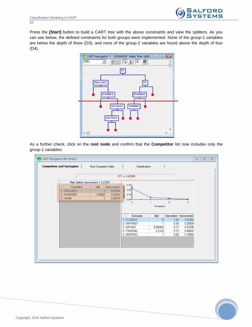
Classification Modeling in CART
56
Copyright, 2016 Salford Systems
Press the [Start] button to build a CART tree with the above constraints and view the splitters. As you
can see below, the defined constraints for both groups were implemented. None of the group-1 variables
are below the depth of three (D3), and none of the group-2 variables are found above the depth of four
(D4).
As a further check, click on the root node and confirm that the Competitor list now includes only the
group-1 variables:

Classification Modeling in CART
57
Copyright, 2016 Salford Systems
575
7
Likewise, the Competitor list in any node below depth 3 includes only the group-2 variables:
Structured Trees using Learn Sample Size
CART also allows the user to constrain a tree according to the size of the learn sample in the nodes.
Instead of using depth to control where a splitter can be used, we disallow splits based on the size of the
learn sample in the node. The “Min Cases” and “Max Cases” columns are used to enter positive values
in the cells:
Min Cases: variable will not be used if the node has more than the specified number of records.
Max Cases: variable will not be used if the node has fewer than the specified number of records.
In the following example we constrain FIT from being used as a splitter unless there are fewer than 200
learn sample observations in a node.

Classification Modeling in CART
58
Copyright, 2016 Salford Systems
Previously, FIT was the root node splitter. Now, it first appears further down the tree once node sizes fall below 200.
Optimal Models and Tree Stability
CART relies on the concept of pruning to create a sequence of nested models as final model candidates.
Independent testing or cross validation is subsequently used to identify the optimal tree with respect to
overall model performance (based on the expected cost criterion). This, however, does not guarantee that
the resulting tree will show stable performance at the node level. It is quite possible to have a node
created earlier in the tree exhibiting unstable behavior across different partitions of the data. Often such
nodes cannot be easily eliminated without picking a much smaller tree in the pruning sequence, thus
picking an inferior (in terms of accuracy) model. Nonetheless, some analysts might be more interested in
finding robust trees with all nodes exhibiting stable behavior and be less concerned with the actual
accuracy measures (for example, marketing segmentation problems). The TTC (Train-Test
Consistency) feature of CART was designed to facilitate such an analysis of the tree sequence.
Spam Data Example
We illustrate the specifics of the TTC feature using the SPAMBASE.CSV dataset.
First, use the Open->Grove File… option from the File menu to open the TTC.GRV command file, that
will automatically build a new model. The resulting Navigator suggests an 18-node tree as the optimal in
terms of expected cost.
Now press the Summary … button and go to the Terminal Nodes tab.

Classification Modeling in CART
59
Copyright, 2016 Salford Systems
595
9
Note two types of instability of the optimal tree with respect to the Learn and Test results:
Directional Instability – Node 15 has 9% of Class=1 on the learn data and 56% of Class=1 on the test
data. Assuming the node majority rule for class assignment, this effectively constitutes instability with
respect to the class assignment that depends on the data partition. Another way to look at this is that the
node lift is less than 1 on the learn data and greater than 1 on the test data.
Rank Instability – The nodes on the graph are sorted according to node richness using the learn data.
However, the sorted order is no longer maintained when looking at the test data; hence, we have another
type of instability. Many deployment strategies (for example, model-guided sampling of subjects in a
direct marketing campaign) rely only on the sorted list of segments and therefore eliminating this kind of
instability is highly desirable.
Note that the Rank Stability requirement is generally stricter than the Directional Stability requirement. In
other words, one may have all nodes directionally stable (agree on the class assignment) and yet have
non-conforming sort orders.
Also note that it is useful to introduce some “slack” in the above comparisons due to limited node sizes.
For example, one might argue that the discrepancies in the sort sequences must be significant enough to
declare the whole model as rank unstable. Similarly, a directional disagreement node must show a
significant difference between learn and test sample estimates. We employ a simple statistical test on a
difference in two population proportions to accomplish this. The z-threshold of this test is controlled by the
user, thus giving varying degrees of slack.
In addition, special care must be taken in handling nodes where the test data is missing entirely (empty
test counts). The user has the option to either declare such trees unstable or to ignore any such node
(Fuzzy Match).

Classification Modeling in CART
60
Copyright, 2016 Salford Systems
Running TTC
To run a TTC analysis just press on the Train vs Test button in the Navigator Window.
As a result you will see the following display. We positioned the display on the optimal (18 nodes) trees
by clicking on appropriate line in Consistency by Trees grid.
The upper half reports stability by trees, one line per tree. You can choose the class of interest by clicking
on the corresponding tab. Green marks stable trees while yellow marks unstable trees. Note that because
there are two different approaches to tree stability (rank or directional), it is possible to have a tree agree
on one criterion and disagree on the other.
The columns in the Consistency by Trees section are:
Tree Name – name of the tree. It is a constant for single trees but will have varying values for automates of CART runs (when applicable).
Terminal Nodes – number of terminal nodes.
Direction Agreement – contains “Agree” if all terminal nodes agree on the direction of classification (within the supplied degree of confidence).
Rank Match – contains “Agree” if all terminal nodes agree on the sorted sequence as described above.

Classification Modeling in CART
61
Copyright, 2016 Salford Systems
616
1
Direction Max-Z – reports the z-value of the standard statistical test on the difference in two population proportions – learn node content versus test node content. Note that a node may agree on the direction (class assignment) but still have a significant difference between the learn and test proportions as reflected by the z-value.
Rank Max-Z – reports the z-value of the standard statistical test on the difference in two population proportions as follows. We first sort nodes by the learn-based responses, then we sort nodes by the test-based responses, and finally we look at the nodes side by side and check the difference in test-based proportions for each pair.
Dir. Fail Count – reports the total number of terminal nodes in the tree that failed directional agreement.
Rank Fail Count – reports the total number of terminal node pairs in the tree that failed the rank agreement.
The Consistency Details by Nodes (lower half) provides a detailed node-by-node stability report for the
tree selected in the Consistency by Trees part (upper half). For example, the optimal tree with 18 terminal
nodes has one directional instability in node 15 (as seen by scrolling the list in the lower half) at the given
significance level.
In addition to the columns already present in the Consistency by Trees report, the following ones are
added:
Lift Learn – node lift on the train data
Lift Test – node lift on the test data
N Focus Learn – number of train records that belong to the focus class in the node
N Focus Test – number of test records that belong to the focus class in the node
N Other Learn – number of train records that do not belong to the focus class in the node
N Other Test – number of test records that do not belong to the focus class in the node
N Node Learn – number of train records in the node
N Node Test – number of test records in the node
You can control which columns are shown and in what order in the Select Columns to Display section.
The following group of controls allows fine user input:
Direction – sets the z-value threshold on the directional stability. A node is declared directionally unstable only if it has contradicting class assignments on learn and test samples and furthermore has the z-value of the corresponding test greater than the threshold. Otherwise, the node is directionally stable (has identical class assignments or z-value is below the threshold).
Rank – sets the z-value threshold on the rank stability. A pair of nodes (taken from learn- and test-based sorted sequences) is declared rank stable if the z-value of the corresponding test is below the threshold.
Fuzzy Match – determines whether empty nodes (on test data) are ignored (Fuzzy Match is pressed) or treated as unstable (Fuzzy Match is not pressed).
Hide Agreed – hides all agreed terminal nodes from the Consistency Details by Nodes report.
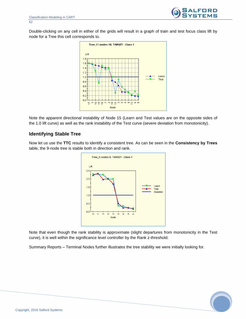
Classification Modeling in CART
62
Copyright, 2016 Salford Systems
Double-clicking on any cell in either of the grids will result in a graph of train and test focus class lift by
node for a Tree this cell corresponds to.
Note the apparent directional instability of Node 15 (Learn and Test values are on the opposite sides of
the 1.0 lift curve) as well as the rank instability of the Test curve (severe deviation from monotonicity).
Identifying Stable Tree
Now let us use the TTC results to identify a consistent tree. As can be seen in the Consistency by Trees
table, the 9-node tree is stable both in direction and rank.
Note that even though the rank stability is approximate (slight departures from monotonicity in the Test
curve), it is well within the significance level controller by the Rank z-threshold.
Summary Reports – Terminal Nodes further illustrates the tree stability we were initially looking for.

Classification Modeling in CART
63
Copyright, 2016 Salford Systems
636
3
Searching for Hot Spots
In many modeling situations an analyst is looking for regions of modeling space richest in the event of
interest. These regions are usually called Hot Spots. For example, in fraud detection problems, we could
be interested in identifying a set of rules that lead to a high ratio of fraud so as to flag records that are
almost guaranteed to be fraudulent. Because target classes usually overlap (making it impossible to have
a clear separation of one target group from the other), a search for hot spots usually results in a reduced
overall accuracy in the class of interest. In other words, while it might be possible to identify areas of data
rich in the event of interest, chances are that a substantial amount of data will be left outside the covered
areas that cannot be easily separated from the remaining class.
One of the advantages of CART is that it gives clear sets of rules describing each terminal node.
Therefore, searching for hot spots usually boils down to searching for nodes richest in the given class
across multiple trees. The hot spot machinery described below can be applied to a single tree, but it is
most beneficial in processing CART automate models (collections of trees obtained by a systematic
change in model settings). While any CART automate can be used, the most suitable for the task is
automate prior. This automate varies the prior probabilities used in tree construction, thus directly
enforcing different requirements in the tradeoff between node richness and class accuracy.
Spam Data Example
We illustrate searching for hot spots using the SPAMBASE.CSV dataset as an example.
First, use the Open->Command File… option from the File menu to open the HOTSPOT.CMD command
file. Note at the bottom of the command file that we will be running automate Priors with priors on class 1
(spam group) varying between 0.5 and 0.9 in increments of 0.02, thus producing 21 models.
✓ See AUTOMATE PRIORS in the command reference as well as the Automation user’s guide.
Second, use the File->Submit Window menu to build the automate. The resulting Automate Results
contains information on all 21 models requested. Our goal is to scan all terminal nodes across all models
and identify the nodes richest in spam.
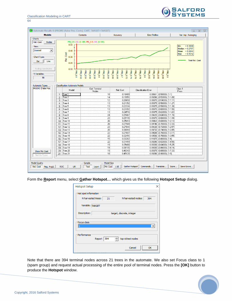
Classification Modeling in CART
64
Copyright, 2016 Salford Systems
Form the Report menu, select Gather Hotspot… which gives us the following Hotspot Setup dialog.
Note that there are 394 terminal nodes across 21 trees in the automate. We also set Focus class to 1
(spam group) and request actual processing of the entire pool of terminal nodes. Press the [OK] button to
produce the Hotspot window.
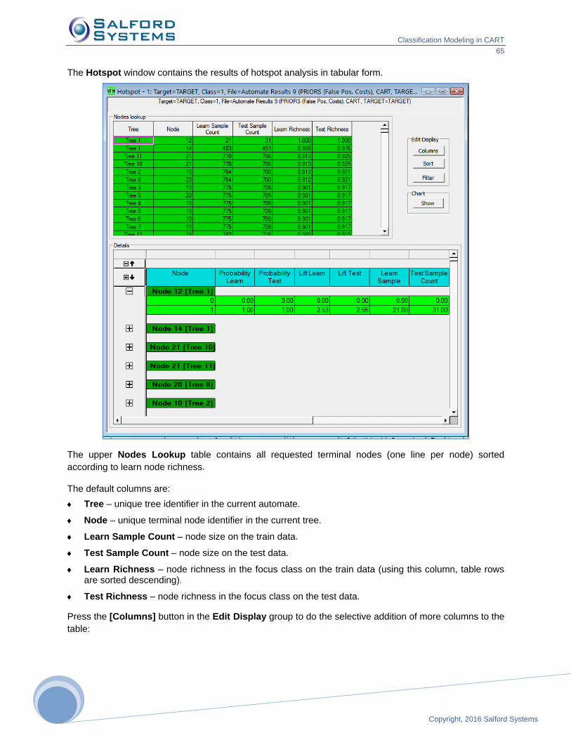
Classification Modeling in CART
65
Copyright, 2016 Salford Systems
656
5
The Hotspot window contains the results of hotspot analysis in tabular form.
The upper Nodes Lookup table contains all requested terminal nodes (one line per node) sorted
according to learn node richness.
The default columns are:
Tree – unique tree identifier in the current automate.
Node – unique terminal node identifier in the current tree.
Learn Sample Count – node size on the train data.
Test Sample Count – node size on the test data.
Learn Richness – node richness in the focus class on the train data (using this column, table rows are sorted descending).
Test Richness – node richness in the focus class on the test data.
Press the [Columns] button in the Edit Display group to do the selective addition of more columns to the
table:

Classification Modeling in CART
66
Copyright, 2016 Salford Systems
Spot – sequential hotspot identifier
Depth – depth level of the node in the tree
Weight Node Learning Count – weighted node size on the train data
Weight Node Test Count – weighted node size on the test data
Focus Class Learning Count – number of focus class records in the node on the train data
Weight Focus Class Learning Count – same as above but weighted
Focus Class Test Count – number of focus class records in the node on the test data
Weight Focus Class Test Count – same as above but weighted
You can change the default sorting method of the nodes using the [Sort] button in the Edit Display group
or introduce your own filtering conditions using the [Filter] button in the same group.
The lower Details part of the table contains additional information on each terminal node, including not
only the focus class but also all the remaining classes.
According to the table, Node 12 of Tree 1 has 100% test richness but only 31 cases. Node 14 of the
same tree is 97.6% rich on a much larger set of 451 test cases. An even larger node (706 test cases) is
found in Tree 11, which has a reduced richness of 92.5%. You can double click on any of the nodes to
request the corresponding navigator window to show up.
If it is not already shown then press the [Show] button to open the Hotspot Chart window:
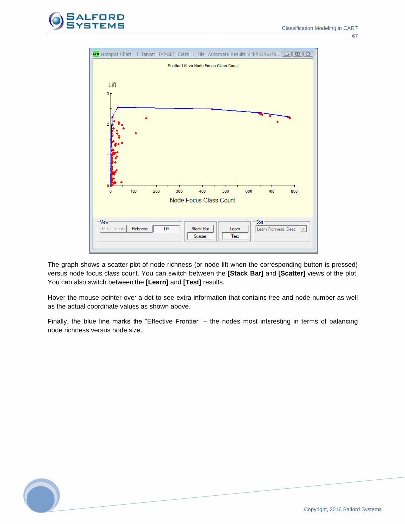
Classification Modeling in CART
67
Copyright, 2016 Salford Systems
676
7
The graph shows a scatter plot of node richness (or node lift when the corresponding button is pressed)
versus node focus class count. You can switch between the [Stack Bar] and [Scatter] views of the plot.
You can also switch between the [Learn] and [Test] results.
Hover the mouse pointer over a dot to see extra information that contains tree and node number as well
as the actual coordinate values as shown above.
Finally, the blue line marks the “Effective Frontier” – the nodes most interesting in terms of balancing
node richness versus node size.

Classification Modeling in CART
68
Copyright, 2016 Salford Systems
Unsupervised Learning and Cluster Analysis
CART in its classification role is an excellent example of "supervised" learning: you cannot start a CART
classification analysis without first selecting a target or dependent variable. All partitioning of the data into
homogenous segments is guided by the primary objective of separating the target classes. If the terminal
nodes are sufficiently pure in a single target class the analysis will be considered successful even if two
or more terminal nodes are similar on most predictor variables.
Unsupervised learning, by contrast, does not begin with a target variable. Instead the objective is to find
groups of similar records in the data. One can think of unsupervised learning as a form of data
compression: we search for a moderate number of representative records to summarize or stand in for
the original database.
Consider a mobile telecommunications company with 20 million customers. The company database will
likely contain various categories of information including customer characteristics such as age and postal
code, product information describing the customer's mobile handset, features of the plan the subscriber
has selected, details of the subscriber's use of plan features, and billing and payment information.
Although it is almost certain that no two subscribers will be identical on every detail in their customer
records, we would expect to find groups of customers who are similar in their overall pattern of
demographics, selected equipment, plan use, and spending and payment behavior. If we could find, say,
30 representative customer types such that the bulk of customers are well described as belonging to their
"type," this information could be very useful for marketing, planning, and new product development.
We cannot promise that we can find clusters or groupings in data that you will find useful, but we include a method quite distinct from that found in other statistical or data mining software. CART and other Salford data mining modules now include an approach to cluster analysis, density estimation and unsupervised learning using ideas that we trace to Leo Breiman, but which may have been known informally among statisticians at Stanford and elsewhere for some time. The method detects structure in data by contrasting original data with randomized variants of that data. Analysts use this method implicitly when viewing data graphically to identify clusters or other structure in data. Take, for example, customer ages and handsets owned. If there were a pattern in the data, we would expect to see certain handsets owned by people in their early 20s and rather different handsets owned by customers in their early 30s. If every handset is just as likely to be owned in every age group then no structure relates these two data dimensions. The method we use generalizes this everyday detection idea to higher dimensions.
The method consists of the following steps:
Make a copy of the original data, and then reorder the data in each column using a random scramble. Do this one column at a time, using a different random ordering for each column, so that no two columns are scrambled in the same way.
Now append the scrambled data set to the original data. We therefore now have the same number of columns as before but twice as many rows. The top portion of the data is the "Original" data and the bottom portion will be the scrambled "Copy." Add a new column to the data to label records by their data source ("Original" vs. "Copy").
Generate a predictive model to attempt to discriminate between the Original and Copy data sets. If it is impossible to tell, after the fact, which records are original and which are random artifacts then there is no structure in the data. If it is easy to tell the difference then there is strong structure in the data.
In the CART model separating the Original from the Copy records, nodes with a high fraction of Original records define regions of high density and qualify as potential "clusters." Such nodes reveal patterns of data values that appear frequently in the real data but not in the randomized artifact.

Classification Modeling in CART
69
Copyright, 2016 Salford Systems
696
9
We do not expect the optimal-sized tree for cluster detection to be the most accurate separator of Original
from Copy records. We recommend that you prune back to a tree size that reveals interesting data
groupings.
This approach to unsupervised learning represents an important advance in clustering technology
because
Variable selection is not necessary and different clusters may be defined on different groups of variables.
Preprocessing or rescaling of the data is unnecessary as these clustering methods are not influenced by how the data are scaled.
Missing values present no challenges because the methods automatically manage missing data.
CART-based clustering gives easy control over the number of clusters and helps select the optimal number.
Setting Up an Unsupervised Model
We will illustrate this special mode of operation using the GOODBAD.CSV dataset. To set up an
unsupervised learning CART run, proceed with the usual steps – opening up a dataset, checking
predictors, setting up other CART parameters, etc.
What makes unsupervised learning run special is that there is no target variable! This is why under the
Target Type you should select Unsupervised.
The Model Setup window will appear:
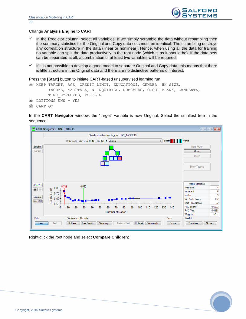
Classification Modeling in CART
70
Copyright, 2016 Salford Systems
Change Analysis Engine to CART
✓ In the Predictor column, select all variables. If we simply scramble the data without resampling then the summary statistics for the Original and Copy data sets must be identical. The scrambling destroys any correlation structure in the data (linear or nonlinear). Hence, when using all the data for training no variable can split the data productively in the root node (which is as it should be). If the data sets can be separated at all, a combination of at least two variables will be required.
✓ If it is not possible to develop a good model to separate Original and Copy data, this means that there is little structure in the Original data and there are no distinctive patterns of interest.
Press the [Start] button to initiate CART-based unsupervised learning run.
KEEP TARGET, AGE, CREDIT_LIMIT, EDUCATION$, GENDER, HH_SIZE,
INCOME, MARITAL$, N_INQUIRIES, NUMCARDS, OCCUP_BLANK, OWNRENT$,
TIME_EMPLOYED, POSTBIN
LOPTIONS UNS = YES
CART GO
In the CART Navigator window, the “target” variable is now Original. Select the smallest tree in the
sequence:
Right-click the root node and select Compare Children:
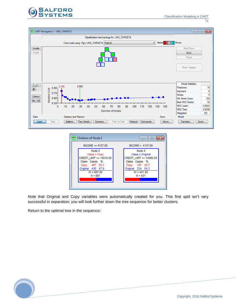
Classification Modeling in CART
71
Copyright, 2016 Salford Systems
717
1
Note that Original and Copy variables were automatically created for you. This first split isn’t very
successful in separation; you will look further down the tree sequence for better clusters.
Return to the optimal tree in the sequence:
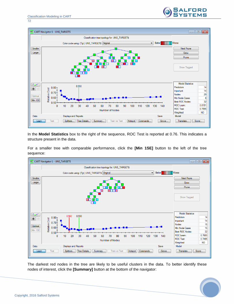
Classification Modeling in CART
72
Copyright, 2016 Salford Systems
In the Model Statistics box to the right of the sequence, ROC Test is reported at 0.76. This indicates a
structure present in the data.
For a smaller tree with comparable performance, click the [Min 1SE] button to the left of the tree
sequence:
The darkest red nodes in the tree are likely to be useful clusters in the data. To better identify these
nodes of interest, click the [Summary] button at the bottom of the navigator:
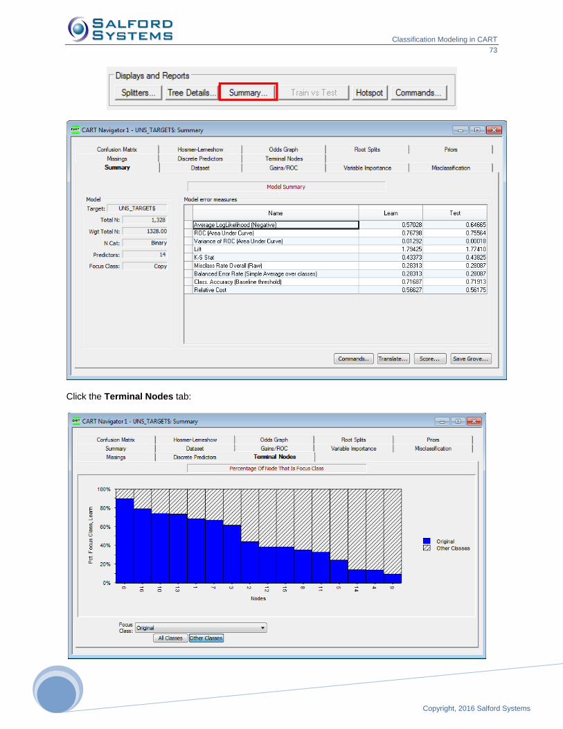
Classification Modeling in CART
73
Copyright, 2016 Salford Systems
737
3
Click the Terminal Nodes tab:
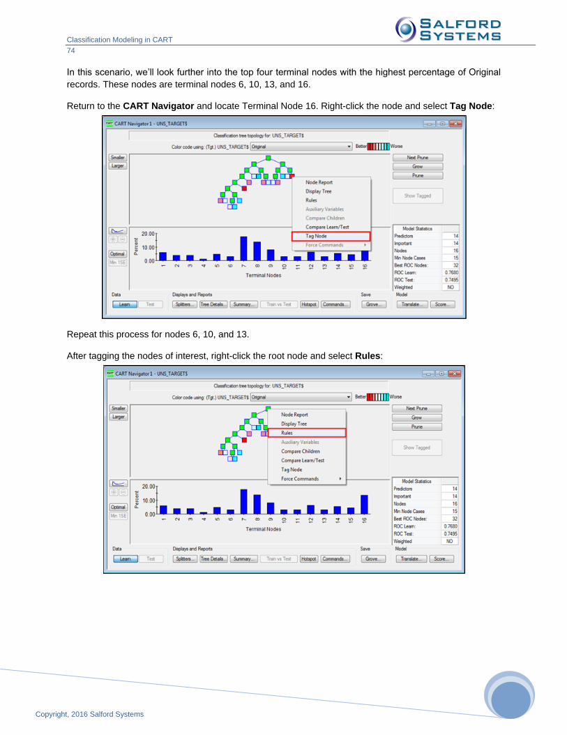
Classification Modeling in CART
74
Copyright, 2016 Salford Systems
In this scenario, we’ll look further into the top four terminal nodes with the highest percentage of Original
records. These nodes are terminal nodes 6, 10, 13, and 16.
Return to the CART Navigator and locate Terminal Node 16. Right-click the node and select Tag Node:
Repeat this process for nodes 6, 10, and 13.
After tagging the nodes of interest, right-click the root node and select Rules:

Classification Modeling in CART
75
Copyright, 2016 Salford Systems
757
5
In the resulting Rules window, click “Tagged” in the Nodes box to only display rules for the tagged nodes.
Here, you will see the conditions for records in each of these nodes. Note, the target variable isn’t
included at all.
For more detailed results of unsupervised learning, see the Unsupervised Learning and Cluster Analysis
section of this manual.