Splines for Diffeomorphic Image Regression

Nikhil Singh and Marc Niethammer

University of North Carolina, Chapel Hill, USA

Abstract. This paper develops a method for splines on diffeomorphismsfor image regression. In contrast to previously proposed methods to cap-ture image changes over time, such as geodesic regression, the methodcan capture more complex spatio-temporal deformations. In particular,it is a first step towards capturing periodic motions for example of theheart or the lung. Starting from a variational formulation of splines theproposed approach allows for the use of temporal control points to controlspline behavior. This necessitates the development of a shooting formu-lation for splines. Experimental results are shown for synthetic and realdata. The performance of the method is compared to geodesic regression.

1 Introduction

With the now common availability of longitudinal and time-series image data,models for their analysis are critically needed. In particular, spatial correspon-dences need to be established through image registration for many medical imageanalysis tasks. While this can be accomplished by pair-wise image registrationto a template image, such an approach neglects spatio-temporal data aspects.Instead, explicitly accounting for spatial and temporal dependencies is desirable.

Methods that generalize Euclidean parametric regression models to mani-folds have proven to be effective for modeling the dynamics of changes rep-resented in time-series of medical images. For instance, methods of geodesicimage regression [6,9] and longitudinal models on images [10] generalize lin-ear and hierarchical linear models, respectively. Although the idea of polynomi-als [5] and splines [11] on landmark representation of shapes have been proposed,these higher-order extensions for image regression remain deficient. While Hin-kle et al. [5] develop general polynomial regression and demonstrate it on finite-dimensional Lie groups, the infinite dimensional regression is demonstrated onlyfor the first-order geodesic image regression.

Contribution. We propose: (a) a shooting based solution to cubic image re-gression in the large deformation (LDDMM) setting, (b) a method of shootingcubic splines as smooth curves to fit complicated shape trends while keepingdata-independent (finite and few) parameters, and (c) a numerically practicalalgorithm for regression of “non-geodesic” medical imaging data. This article isstructured as follows: § 2 reviews the variational approach to splines in Euclideanspace and motivate its shooting formulation for parametric regression. § 3 thengeneralizes this concept of shooting splines for diffeomorphic image regression.We discuss experimental results in § 4.

2 Shooting-splines in the Euclidean Case

Variational formulation. An acceleration controlled curve with time-dependentstates, (x1, x2, x3) such that, x2 = x1 and x3 = x2, defines a cubic curve in Eu-

clidean spaces. This curve minimizes an energy of the form, E = 12

∫ 1

0‖x3‖2dt,

and solves an underlying constrained optimization problem,

minimizex1,x2,x3

E(x3) subject to x2 = x1 and x3 = x2. (1)

Here x3 is referred to as the control variable that describes the acceleration ofthe dynamics in this system. The unconstrained Lagrangian for the above is,

E(x1, x2, x3, µ1, µ2) =1

2

∫ 1

0

‖x3‖2dt+

∫ 1

0

µT1 (x1 − x2)dt+

∫ 1

0

µT2 (x2 − x3)dt,

where µ1 and µ2 are the time-dependent Lagrangian variables or the adjointvariables (also called duals) that enforce the dynamic constraints. Optimalityconditions on the gradients of the above Lagrangian with respect to the states,(x1, x2, x3), result in the adjoint system of equations, µ1 = 0 and x3 = −µ1 (µ2

gets eliminated). This allows for a relaxation solution to Eq. (1).From relaxation to shooting. We write the shooting formulation by explicitlyadding the evolution of x3, obtained by solving the relaxation problem, as adynamical constraint. This increases the order of the dynamics. Denoting, x4 =−µ1, results in the classical system of equations for shooting cubic curves,

x1 = x2(t), x2 = x3(t), x3 = x4(t), x4 = 0. (2)

The states, (x1, x2, x3, x4), at all times, are entirely determined by their initial

values (x01, x02, x

03, x

04), and in particular, x1(t) = x01 + x02t+

x03

2 t2 +

x04

6 t3.

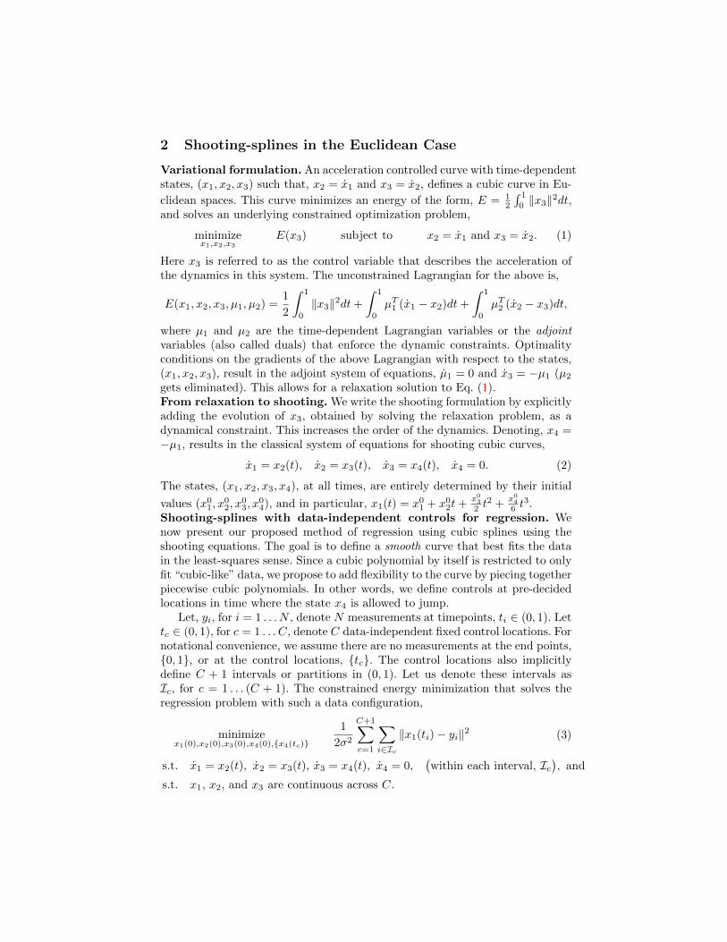
Shooting-splines with data-independent controls for regression. Wenow present our proposed method of regression using cubic splines using theshooting equations. The goal is to define a smooth curve that best fits the datain the least-squares sense. Since a cubic polynomial by itself is restricted to onlyfit “cubic-like” data, we propose to add flexibility to the curve by piecing togetherpiecewise cubic polynomials. In other words, we define controls at pre-decidedlocations in time where the state x4 is allowed to jump.

Let, yi, for i = 1 . . . N , denote N measurements at timepoints, ti ∈ (0, 1). Lettc ∈ (0, 1), for c = 1 . . . C, denote C data-independent fixed control locations. Fornotational convenience, we assume there are no measurements at the end points,0, 1, or at the control locations, tc. The control locations also implicitlydefine C + 1 intervals or partitions in (0, 1). Let us denote these intervals asIc, for c = 1 . . . (C + 1). The constrained energy minimization that solves theregression problem with such a data configuration,

minimizex1(0),x2(0),x3(0),x4(0),x4(tc)

1

2σ2

C+1∑c=1

∑i∈Ic

‖x1(ti)− yi‖2 (3)

s.t. x1 = x2(t), x2 = x3(t), x3 = x4(t), x4 = 0,(within each interval, Ic

), and

s.t. x1, x2, and x3 are continuous across C.

0.0 0.2 0.4 0.6 0.8 1.0t

1.0

0.5

0.0

0.5

1.0

1.5

Noisy data

Estimated x1

0.0 0.2 0.4 0.6 0.8 1.0t

15

10

5

0

5

10

15

Estimated x2

0.0 0.2 0.4 0.6 0.8 1.0t

120

100

80

60

40

20

0

20

40

60

Estimated x3

0.0 0.2 0.4 0.6 0.8 1.0t

400

300

200

100

0

100

200

300

400

Estimated x4

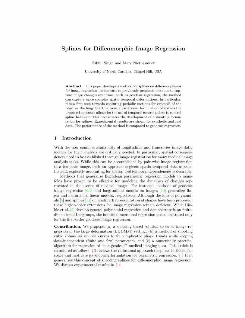
Fig. 1: States for splines regression in Euclidean space with one control at t=0.5.

The unconstrained Lagrangian enforcing shooting and continuity constraints us-ing time-dependent adjoint states, (λ1, λ2, λ3, λ4), and duals, (ν1, ν2, ν3), is

E(x01, x02,x

03, x

04, x

tc4 , λ1, λ2, λ3, λ4) =

1

2σ2

C+1∑c=1

∑i∈Ic

‖x1(ti)− yi‖2

+

∫ 1

0

(λT1 (x1 − x2) + λT2 (x2 − x3) + λT3 (x3 − x4) + λT4 x4

)dt

+ ν1(x−1 (tc)− x+1 (tc)) + ν2(x−2 (tc)− x+2 (tc)) + ν3(x−3 (tc)− x+3 (tc)).

The conditions of optimality on the gradients of the above Lagrangian resultin the adjoint system of equations, λ1 = 0, λ2 = −λ1, λ3 = −λ2, λ4 = −λ3.The gradients with respect to the initial conditions for states x0l for l = 1, . . . , 4are, δx0

1E = −λ1(0), δx0

2E = −λ2(0), δx0

3E = −λ3(0) and δx0

4E = −λ4(0).

The jerks at controls, xtc4 , are updated using, δxtc4E = −λ4(tc). The values

of adjoint variables required in these gradients are computed by integratingbackward the adjoint system. Note that λ1, λ2 and λ3 are continuous at joins,but λ1 jumps at the data-point location as per, λ1(t+i )−λ1(t−i ) = 1

σ2 (x1(ti)−yi).During backward integration, λ4 starts from zero at each interval at tc+1 andthe accumulated value at tc is used for the gradient update of x4(tc).

It is critical to note that, along the time, t, such a formulation guaranteesthat: (a) x4(t) is piecewise constant, (b) x3(t) is piecewise linear, (c) x2(t) ispiecewise quadratic, and (d) x1(t) is piecewise cubic. Thus, this results in acubic-spline curve. Fig. 1 demonstrates this shooting spline fitting on scalar data.While it is not possible to explain this data with a simple cubic curve alone, itsuffices to allow one control location to recover the meaningful underlying trend.The state, x4, experiences a jump at the control location that integrates upthrice to give a C2-continuous evolution for the state, x1.

3 Shooting-splines for Diffeomorphisms

Notations and preliminaries. We denote the group of diffeomorphisms by Gand its elements by g; the tangent space at g by TgG; and the Lie algebra, TeG,by g. Let Ω be the coordinate space of the image, I. A diffeomorphism, g(t), is

constructed by integrating an ordinary differential equation (ODE) on Ω definedvia a smooth, time-indexed velocity field, v(t). The deformation of an image Iby g is defined as the action of the diffeomorphism, given by g · I = I g−1. Thechoice of a self-adjoint differential operator, L, determines the right-invariantRiemannian structure on the collection of velocity fields with the norm definedas, ‖v‖2g =

∫Ω

(Lv(x), v(x))dx. The velocity, v ∈ g, maps to its dual deformationmomenta, m ∈ g∗, via the operator L such that m = Lv and v = K ? m. Theoperator K : g∗ → g denotes the inverse of L. For a thorough review of theRiemannian structure on the group of diffeomorphisms, please refer to [12,1,13].Variational formulation. As an end-point problem, a Riemannian cubic splineis defined by the curve g(t), that minimizes an energy of the form, E(g) =12

∫ 1

0‖∇g g‖2TgG

dt, where ∇ denotes the Levi-Civita connection and ‖ · ‖TgG isthe metric on the manifold at g. The quantity, ∇g g, is the generalization ofthe idea of acceleration to Riemannian manifolds [7,3]. Another way to definethe spline is by defining a time dependent control that forces the curve g(t) todeviate from being a geodesic [11]. Such a control or a forcing variable, u(t),takes the form, ∇g(t)g(t) = u(t). Notice, u(t) = 0 implies that g(t) is a geodesic.

Taking this idea forward to the group of diffeomorphisms, G, we propose toinclude a time-dependent forcing term that describes how much the ‘geodesic re-quirement’ deviates. Thus, we define the control directly on the known momentaEPDiff evolution equation for geodesics[13], obtained using the right invariantmetric to give the evolution in Lie algebra, g, as m+ ad∗vm = 0. Here, the oper-ator ad∗ is the adjoint of the Jacobi-Lie bracket [2,13]. After adding this control,the dynamics take the form, m + ad∗vm = u, where u ∈ g∗. Thus we allow thegeodesic to deviate from satisfying the EPDiff constraints and constrain it to

minimize an energy of the form, E = 12

∫ 1

0‖u(t)‖2gdt. It is important to note that

such a formulation will avoid direct computation of curvature. In other words,since the Levi-Civita connection is expressed in terms of curvature, we bypass itwhen we control the EPDiff in g instead of controlling ∇g(t)g(t) in Tg(t)G.

The constrained energy minimization problem for splines is,

minimizeu

1

2

∫ 1

0

‖u(t)‖2gdt

subject to control u(t)− m(t)− ad∗v(t)m(t) = 0,

subject to right action g(t) = v g(t),

subject to image evolution I(t) = I(0) g−1(t),

subject to momenta duality v(t) = K ?m(t).

(4)

Similar to the Euclidean case, the Euler-Lagrange equations for the above op-timization problem give an adjoint system that explains the evolution of u, orequivalently its dual, f ∈ g (f = K?u), such that, f−K?PDI+ad†f v−adv f = 0,

and P +∇· (Pv) = 0. Here, P is the adjoint variable corresponding to the image

evolution constraint and the conjugate operator is, ad†X(·) = K ? adX L(·).From relaxation to shooting. Notice that the above discussion is analogousto the discussion of the relaxation formulation for the Euclidean case in the

sense that the Euclidean states (x1, x2, x3) 7→ (g, v, f) in diffeomorphisms. Wenow convert the adjoint state, P (t) to a primal state to form a forward shootingsystem. Analogous to the Euclidean case, this increases the order of the systemby one. The shooting system for acceleration controlled motion is

g − v g = 0, v − f + ad†v v = 0,

f −K ? PDI + ad†f v − adv f = 0, P +∇ · (Pv) = 0.

The image evolves (equivalently advects) as per the group action of g on I(0).Here, the vector quantity, K ? PDI is analogous to x4.Shooting-splines with data-independent controls for regression. Similarto the data configuration in the Euclidean example, in the context of regression,let, Ji, for i = 1 . . . N , denote N measured images at timepoints, ti ∈ (0, 1).The goal now is to define finite and relatively fewer points than the number ofmeasurements in the interval, (0, 1) where K ?PDI is allowed to jump. In otherwords, P does not jump at every measurement but instead, is allowed to be freeat predefined time-points that are decided independently of the data. Thus, weconstruct a curve g(t), similar to the Euclidean case, in G, along the time, t,such that it guarantees, (a) K ? PDI is not continuous, (b) f is C0-continuous,(c) v is C1-continuous, and (d) g is C2-continuous.

The unconstrained Lagrangian for spline regression takes the form:

E(m0, u0, P 0, I0, P tc , λm, λu, λP , λI) =1

2σ2

C+1∑c=1

∑i∈Ic

‖I(ti)− Ji‖2 (5)

+

C+1∑c=1

∫ 1

0

〈λmc, mc − uc + ad∗vc mc〉+ 〈λuc, u− PcDIc + ad∗fc mc −K−1 advc fc〉dt

+

C+1∑c=1

∫ 1

0

〈λPc, Pc +∇ · (Pcvc)〉+ 〈λIc, Ic +DIc · vc〉+ 〈λvc, vc −K ?mc〉dt

+

C+1∑c=1

∫ 1

0

〈λfc, fc −K ? uc〉dt+ subject to continuity of m, u, and I at C joins.

Gradients. The optimality conditions on the gradients of the above energyfunctional show that the adjoint variables, λm, λu, λI , are continuous at all Cjoins. The gradients with respect to the initial conditions are,

δm01E = −λm1(0), δu0

1E = −λu1(0), δP 0

1E = −λP1(0), δI01E = −λI1(0).

We compute the gradients by integrating the adjoint system of equations withineach interval backward in time,

λmc + adλmcvc + ad†λmc

vc − adfc λuc− ad†fc λuc −K ? λIcDIc = 0, (6)

λuc + λmc + ad†λucvc + ad†vc λuc = 0, (7)

λPc +DIc · λuc +DλPc · vc = 0, (8)

λIc +∇ · (λIcvc)−∇ · (Pcλuc) = 0. (9)

All variables start from zero as their initial conditions for this backwardintegration. Similar to the Euclidean case, we add jumps in λI as λIc(t

+i ) −

λIc(t−i ) = 1

σ2 (Ic(ti) − Ji) at measurements, t = ti. We ensure the continuity ofλmc, λuc, and λIc at the joins and λPc starts from zero at every join. We usethe accumulated λPc+1 to update the jerk, Pc(tk), at the control location with,

δPc+1(tc)(tc)E = −λPc+1(tc). (10)

Note this is the ‘data independent’ control that we motivated our formulationwith. This determines the initial condition of the forward system for each intervaland needs to be estimated numerically. Also note that a regularizer can be addedon the initial momenta, m0

1 by restricting its Sobolev norm, in which case, thegradient includes an additional term and takes the form, δm0

1E = Km0

1−λm1(0).

4 Results and Discussion

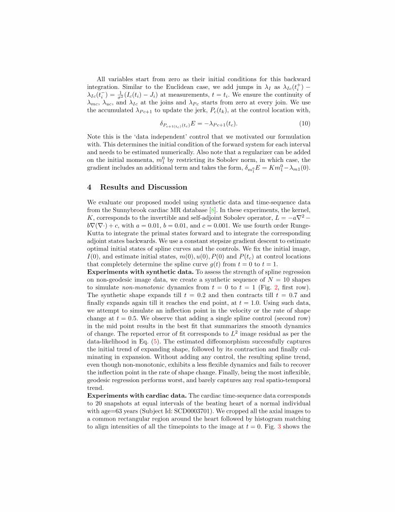
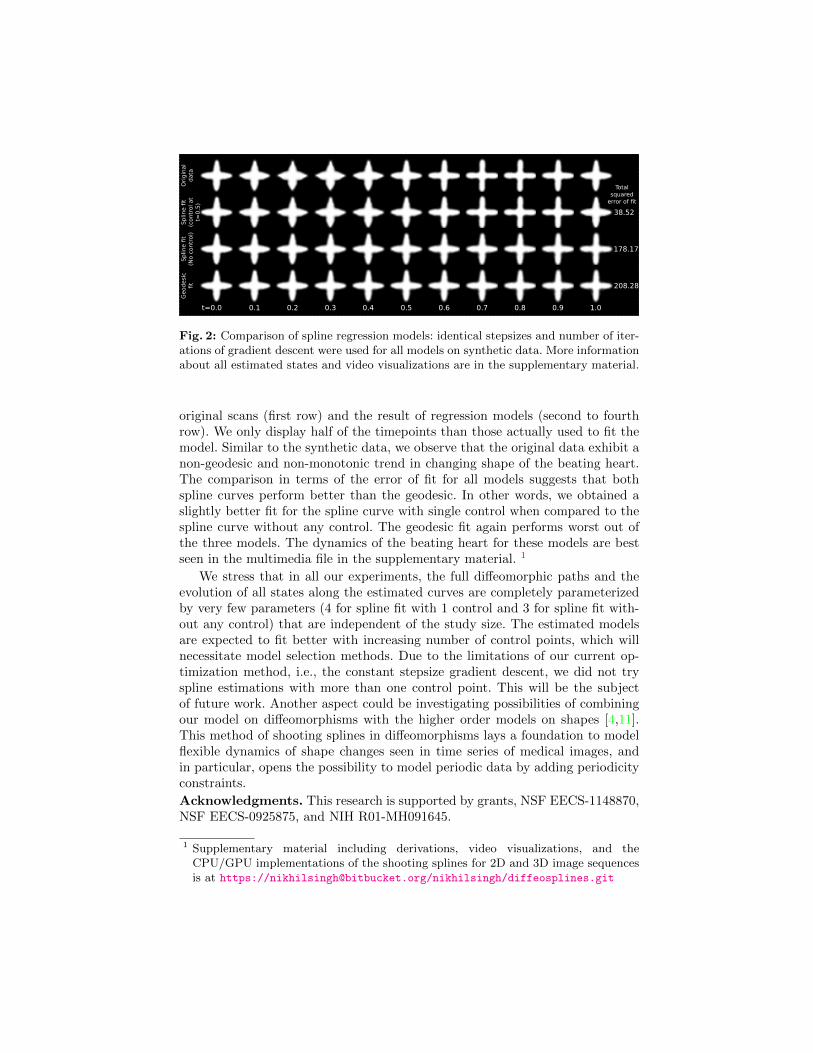
We evaluate our proposed model using synthetic data and time-sequence datafrom the Sunnybrook cardiac MR database [8]. In these experiments, the kernel,K, corresponds to the invertible and self-adjoint Sobolev operator, L = −a∇2−b∇(∇·) + c, with a = 0.01, b = 0.01, and c = 0.001. We use fourth order Runge-Kutta to integrate the primal states forward and to integrate the correspondingadjoint states backwards. We use a constant stepsize gradient descent to estimateoptimal initial states of spline curves and the controls. We fix the initial image,I(0), and estimate initial states, m(0), u(0), P (0) and P (tc) at control locationsthat completely determine the spline curve g(t) from t = 0 to t = 1.Experiments with synthetic data. To assess the strength of spline regressionon non-geodesic image data, we create a synthetic sequence of N = 10 shapesto simulate non-monotonic dynamics from t = 0 to t = 1 (Fig. 2, first row).The synthetic shape expands till t = 0.2 and then contracts till t = 0.7 andfinally expands again till it reaches the end point, at t = 1.0. Using such data,we attempt to simulate an inflection point in the velocity or the rate of shapechange at t = 0.5. We observe that adding a single spline control (second row)in the mid point results in the best fit that summarizes the smooth dynamicsof change. The reported error of fit corresponds to L2 image residual as per thedata-likelihood in Eq. (5). The estimated diffeomorphism successfully capturesthe initial trend of expanding shape, followed by its contraction and finally cul-minating in expansion. Without adding any control, the resulting spline trend,even though non-monotonic, exhibits a less flexible dynamics and fails to recoverthe inflection point in the rate of shape change. Finally, being the most inflexible,geodesic regression performs worst, and barely captures any real spatio-temporaltrend.Experiments with cardiac data. The cardiac time-sequence data correspondsto 20 snapshots at equal intervals of the beating heart of a normal individualwith age=63 years (Subject Id: SCD0003701). We cropped all the axial images toa common rectangular region around the heart followed by histogram matchingto align intensities of all the timepoints to the image at t = 0. Fig. 3 shows the

Ori

gin

al

data

Splin

e fi

t(c

ontr

ol at

t=0

.5)

Geodesi

cfit

Splin

e fi

t(N

o c

ontr

ol)

Totalsquared

error of fit

t=0.0 0.1 0.2 0.3 0.4 0.5 0.6 0.7 0.8 0.9 1.0

38.52

178.17

208.28

Fig. 2: Comparison of spline regression models: identical stepsizes and number of iter-ations of gradient descent were used for all models on synthetic data. More informationabout all estimated states and video visualizations are in the supplementary material.

original scans (first row) and the result of regression models (second to fourthrow). We only display half of the timepoints than those actually used to fit themodel. Similar to the synthetic data, we observe that the original data exhibit anon-geodesic and non-monotonic trend in changing shape of the beating heart.The comparison in terms of the error of fit for all models suggests that bothspline curves perform better than the geodesic. In other words, we obtained aslightly better fit for the spline curve with single control when compared to thespline curve without any control. The geodesic fit again performs worst out ofthe three models. The dynamics of the beating heart for these models are bestseen in the multimedia file in the supplementary material. 1

We stress that in all our experiments, the full diffeomorphic paths and theevolution of all states along the estimated curves are completely parameterizedby very few parameters (4 for spline fit with 1 control and 3 for spline fit with-out any control) that are independent of the study size. The estimated modelsare expected to fit better with increasing number of control points, which willnecessitate model selection methods. Due to the limitations of our current op-timization method, i.e., the constant stepsize gradient descent, we did not tryspline estimations with more than one control point. This will be the subjectof future work. Another aspect could be investigating possibilities of combiningour model on diffeomorphisms with the higher order models on shapes [4,11].This method of shooting splines in diffeomorphisms lays a foundation to modelflexible dynamics of shape changes seen in time series of medical images, andin particular, opens the possibility to model periodic data by adding periodicityconstraints.

Acknowledgments. This research is supported by grants, NSF EECS-1148870,NSF EECS-0925875, and NIH R01-MH091645.

1 Supplementary material including derivations, video visualizations, and theCPU/GPU implementations of the shooting splines for 2D and 3D image sequencesis at https://nikhilsingh@bitbucket.org/nikhilsingh/diffeosplines.git

Ori

gin

al

data

Sp

line fi

t(c

ontr

ol at

t=0

.5)

Geod

esi

cfit

Sp

line fi

t(N

o c

ontr

ol)

Totalsquared

error of fit

t=0.0 0.1 0.2 0.3 0.4 0.5 0.6 0.7 0.8 0.9 1.0

424.96

479.00

660.33

Fig. 3: Spline regression models on cardiac MRI breathing data. Comparison is betterseen in the video visualizations in supplementary material.

References

1. Arnol’d, V.I.: Sur la geometrie differentielle des groupes de Lie de dimension infinieet ses applications a l’hydrodynamique. Ann. Inst. Fourier 16, 319–361 (1966) 3

2. Bruveris, M., Gay-Balmaz, F., Holm, D., Ratiu, T.: The momentum map repre-sentation of images. Journal of Nonlinear Science 21(1), 115–150 (2011) 3

3. Camarinha, M., Leite, F.S., Crouch, P.: Splines of class ck on non-euclidean spaces.IMA Journal of Mathematical Control and Information 12(4), 399–410 (1995) 3

4. Gay-Balmaz, F., Holm, D.D., Meier, D.M., Ratiu, T.S., Vialard, F.X.: Invarianthigher-order variational problems II. J. Nonlinear Science 22(4), 553–597 (2012) 4

5. Hinkle, J., Fletcher, P., Joshi, S.: Intrinsic polynomials for regression on Rieman-nian manifolds. Journal of Mathematical Imaging and Vision pp. 1–21 (2014) 1

6. Niethammer, M., Huang, Y., Vialard, F.X.: Geodesic regression for image time-series. In: Fichtinger, G., Martel, A., Peters, T. (eds.) MICCAI 2011, LNCS, vol.6892, pp. 655–662. Springer Berlin Heidelberg (2011) 1

7. Noakes, L., Heinzinger, G., Paden, B.: Cubic splines on curved spaces. IMA Journalof Mathematical Control and Information 6(4), 465–473 (1989) 3

8. Radau, P., Lu, Y., Connelly, K., Paul, G., Dick, A., Wright, G.: Evaluation frame-work for algorithms segmenting short axis cardiac MRI. (07 2009) 4

9. Singh, N., Hinkle, J., Joshi, S., Fletcher, P.: A vector momenta formulation ofdiffeomorphisms for improved geodesic regression and atlas construction. In: ISBI.pp. 1219–1222 (2013) 1

10. Singh, N., Hinkle, J., Joshi, S., Fletcher, P.: A hierarchical geodesic model fordiffeomorphic longitudinal shape analysis. In: IPMI, vol. 7917, pp. 560–571 (2013)1

11. Trouve, A., Vialard, F.X.: Shape splines and stochastic shape evolutions: A secondorder point of view. Quarterly of Applied Mathematics 70(2), 219–251 (2012) 1,3, 4

12. Younes, L.: Shapes and Diffeomorphisms, vol. 171. Springer Berlin (2010) 313. Younes, L., Arrate, F., Miller, M.I.: Evolution equations in computational anatomy.

NeuroImage 45(1 Suppl), S40–S50 (2009) 3