SPIRAL: A Generator for Platform-Adapted Librariesof Signal Processing Algorithms

Markus Puschel∗ Bryan Singer Jianxin Xiong Jose M. F. MouraJeremy Johnson David Padua Manuela Veloso Robert W. Johnson

Abstract

SPIRAL is a generator of libraries of fast software implementations of linear signal processing trans-forms. These libraries are adapted to the computing platform and can be re-optimized as the hardware isupgraded or replaced. This paper describes the main components of SPIRAL: the mathematical frame-work that concisely describes signal transforms and their fast algorithms; the formula generator thatcaptures at the algorithmic level the degrees of freedom in expressing a particular signal processingtransform; the formula translator that encapsulates the compilation degrees of freedom when translatinga specific algorithm into an actual code implementation; and, finally, an intelligent search engine thatfinds within the large space of alternative formulas and implementations the “best” match to the givencomputing platform. We present empirical data that demonstrates the high performance of SPIRALgenerated code.

1 Introduction

The short life cycles of modern computer platforms are a major problem for developers of high performancesoftware for numerical computations. The different platforms are usually source code compatible (i.e., asuitably written C program can be recompiled) or even binary compatible (e.g., if based on Intel’s x86architecture), but the fastest implementation is platform-specific due to differences in, for example, microar-chitectures or cache sizes and structures. Thus, producing optimal code requires skilled programmers withintimate knowledge in both the algorithms and the intricacies of the target platform. When the computingplatform is replaced, hand-tuned code becomes obsolete.

The need to overcome this problem has led in recent years to a number of research activities that arecollectively referred to as “automatic performance tuning.” These efforts target areas with high performancerequirements such as very large data sets or real time processing.

One focus of research has been the area of linear algebra leading to highly efficient automatically tunedsoftware for various algorithms. Examples include ATLAS [36], PHiPAC [2], and SPARSITY [17].

Another area with high performance demands is digital signal processing (DSP), which is at the heartof modern telecommunications and is an integral component of different multi-media technologies, such asimage/audio/video compression and water marking, or in medical imaging like computed image tomographyand magnetic resonance imaging, just to cite a few examples. The computationally most intensive tasksin these technologies are performed by discrete signal transforms. Examples include the discrete Fouriertransform (DFT), the discrete cosine transforms (DCTs), the Walsh-Hadamard transform (WHT) and thediscrete wavelet transform (DWT).

∗This work was supported by DARPA through research grant DABT63-98-1-0004 administered by the Army Directorate ofContracting.

1

The research on adaptable software for these transforms has to date been comparatively scarce, exceptfor the efficient DFT package FFTW [11, 10]. FFTW includes code modules, called “codelets,” for smalltransform sizes, and a flexible breakdown strategy, called a “plan,” for larger transform sizes. The codeletsare distributed as a part of the package. They are automatically generated and optimized to perform well onevery platform, i.e., they are not platform-specific. Platform-adaptation arises from the choice of plan, i.e.,how a DFT of large size is recursively reduced to smaller sizes. FFTW has been used by other groups totest different optimization techniques, such as loop interleaving [13], and the use of short vector instructions[7]; UHFFT [21] uses an approach similar to FFTW and includes search on the codelet level and additionalrecursion methods.

SPIRAL is a generator for platform-adapted libraries of DSP transforms, i.e., it includes no code forthe computation of transforms prior to installation time. The users trigger the code generation process afterinstallation by specifying the transforms to implement. In this paper we describe the main components ofSPIRAL: the mathematical framework to capture transforms and their algorithms, the formula generator,the formula translator, and the search engine.

SPIRAL’s design is based on the following realization:• DSP transforms have a very large number of different fast algorithms (the term “fast” refers to the oper-

ations count).• Fast algorithms for DSP transforms can be represented as formulas in a concise mathematical notation

using a small number of mathematical constructs and primitives.• In this representation, the different DSP transform algorithms can be automatically generated.• The automatically generated algorithms can be automatically translated into a high-level language (like

C or Fortran) program.Based on these facts, SPIRAL translates the task of finding hardware adapted implementations into an

intelligent search in the space of possible fast algorithms and their implementations.The main difference to other approaches, in particular to FFTW, is the concise mathematical represen-

tation that makes the high-level structural information of an algorithm accessible within the system. Thisrepresentation, and its implementation within the SPIRAL system, enables the automatic generation of thealgorithm space, the high-level manipulation of algorithms to apply various search methods for optimiza-tion, the systematic evaluation of coding alternatives, and the extension of SPIRAL to different transformsand algorithms. The details will be provided in Sections 2–4.

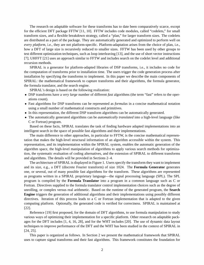
The architecture of SPIRAL is displayed in Figure 1. Users specify the transform they want to implementand its size, e.g., a DFT (discrete Fourier transform) of size 1024. The Formula Generator generatesone, or several, out of many possible fast algorithms for the transform. These algorithms are representedas programs written in a SPIRAL proprietary language—the signal processing language (SPL). The SPLprogram is compiled by the Formula Translator into a program in a common language such as C orFortran. Directives supplied to the formula translator control implementation choices such as the degree ofunrolling, or complex versus real arithmetic. Based on the runtime of the generated program, the SearchEngine triggers the generation of additional algorithms and their implementations using possibly differentdirectives. Iteration of this process leads to a C or Fortran implementation that is adapted to the givencomputing platform. Optionally, the generated code is verified for correctness. SPIRAL is maintained at[22].

Reference [19] first proposed, for the domain of DFT algorithms, to use formula manipulation to studyvarious ways of optimizing their implementation for a specific platform. Other research on adaptable pack-ages for the DFT includes [1, 4, 16, 28], and for the WHT includes [20]. The use of dynamic data layouttechniques to improve performance of the DFT and the WHT has been studied in the context of SPIRAL in[24, 25].

This paper is organized as follows. In Section 2 we present the mathematical framework that SPIRALuses to capture signal transforms and their fast algorithms. This framework constitutes the foundation for

2

DSP transform (user specified)

?

Formula Translator

?

Formula Generator

Sear

chE

ngin

e�controls

algorithm generation

�controls

implementation options

fast algorithmas SPL formula

6runtime on given platform

platform-adapted implementation?

Figure 1: The architecture of SPIRAL.

SPIRAL’s architecture. The following three sections explain the three main components of SPIRAL, theformula generator (Section 3), the formula translator (Section 4), and the search engine (Section 5). Sec-tion 6 presents empirical runtime results for the code generated by SPIRAL. For most transforms, highlytuned code is not readily available as benchmark. An exception is the DFT for which we compared SPIRALgenerated code with FFTW, one of the fastest FFT packages available.

2 SPIRAL’s Framework

SPIRAL captures linear discrete signal transforms (also called DSP transforms) and their fast algorithms ina concise mathematical framework. The transforms are expressed as a matrix-vector product

y = M · x, (1)

where x is a vector of n data points, M is an n×n matrix representing the transform, and y is the transformedvector.

Fast algorithms for signal transforms arise from factorizations of the transform matrix M into a productof sparse matrices,

M = M1 ·M2 · · ·Mt, Mi sparse. (2)

Typically, these factorizations reduce the arithmetic cost of computing the transform from O(n2), as requiredby direct matrix-vector multiplication, to O(n log n). It is a special property of signal transforms that thesefactorizations exist and that the matrices Mi are highly structured. In SPIRAL, we use this structure to writethese factorizations in a very concise form.

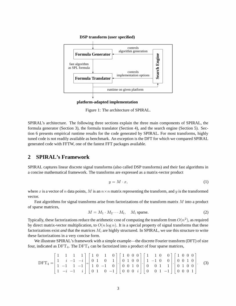
We illustrate SPIRAL’s framework with a simple example—the discrete Fourier transform (DFT) of sizefour, indicated as DFT4. The DFT4 can be factorized into a product of four sparse matrices,

DFT4 =

1 1 1 11 i −1 −i1 −1 1 −11 −i −1 i

=

1 0 1 00 1 0 11 0 −1 00 1 0 −1

·

1 0 0 00 1 0 00 0 1 00 0 0 i

·

1 1 0 01 −1 0 00 0 1 10 0 1 −1

·

1 0 0 00 0 1 00 1 0 00 0 0 1

. (3)

3

This factorization represents a fast algorithm for computing the DFT of size four and is an instantiation ofthe Cooley-Tukey algorithm [3], usually referred to as the fast Fourier transform (FFT). Using the structureof the sparse factors, (3) is rewritten in the concise form

DFT4 = (DFT2⊗ I2) · T42 · (I2⊗DFT2) · L4

2, (4)

where we used the following notation. The tensor (or Kronecker) product of matrices is defined by

A⊗B = [ak,` ·B], where A = [ak,`].

The symbols In, Lrsr , Trs

r represent, respectively, the n × n identity matrix, the rs × rs stride permutationmatrix that maps the vector element indices j as

Lrsr : j 7→ j · r mod rs− 1, for j = 0, . . . , rs− 2; rs− 1 7→ rs− 1, (5)

and the diagonal matrix of twiddle factors (n = rs),

Trsr =

s−1⊕

j=0

diag(ω0n, . . . , ωr−1

n )j , ωn = e2πi/n, i =√−1, (6)

where

A⊕B =

[A

B

]

denotes the direct sum of A and B. Finally,

DFT2 =

[1 11 −1

]

is the DFT of size 2.A good introduction to the matrix framework of FFT algorithms is provided in [32, 31]. SPIRAL extends

this framework 1) to capture the entire class of linear DSP transforms and their fast algorithms; and 2) toprovide the formalism necessary to automatically generate these fast algorithms. We now extend the simpleexample above and explain SPIRAL’s mathematical framework in detail. In Section 2.1 we define theconcepts that SPIRAL uses to capture transforms and their fast algorithms. Section 2.2 introduces a numberof different transforms considered by SPIRAL. Section 2.3 discusses the space of different algorithms for agiven transform. Finally, Section 2.4 explains how SPIRAL’s architecture (see Figure 1) is derived from thepresented framework.

2.1 Transforms, Rules, and Formulas

In this section we explain how DSP transforms and their fast algorithms are captured by SPIRAL. At theheart of our framework are the concepts of rules and formulas. In short, rules are used to expand a giventransform into formulas, which represent algorithms for this transform. We will now define these conceptsand illustrate them using the DFT.

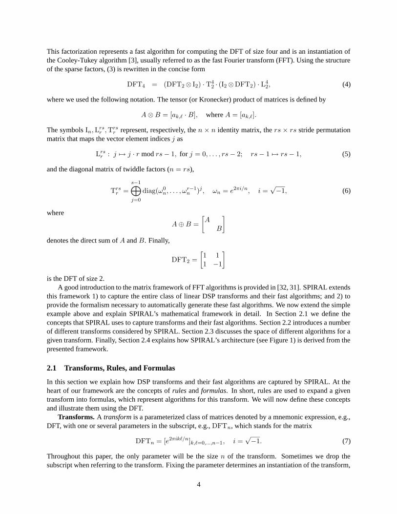
Transforms. A transform is a parameterized class of matrices denoted by a mnemonic expression, e.g.,DFT, with one or several parameters in the subscript, e.g., DFTn, which stands for the matrix

DFTn = [e2πik`/n]k,`=0,...,n−1, i =√−1. (7)

Throughout this paper, the only parameter will be the size n of the transform. Sometimes we drop thesubscript when referring to the transform. Fixing the parameter determines an instantiation of the transform,

4

e.g., DFT8 by fixing n = 8. By abuse of notation, we will refer to an instantiation also as a transform. Bycomputing a transform M , we mean evaluating the matrix-vector product y = M · x in Equation (1).

Rules. A break-down rule, or simply rule, is an equation that structurally decomposes a transform. Theapplicability of the rule may depend on the parameters, i.e., the size of the transform. An example rule isthe Cooley-Tukey FFT for a DFTn, given by

DFTn = (DFTr ⊗ Is) · Tns ·(Ir ⊗DFTs) · Ln

r , for n = r · s, (8)

where the twiddle matrix Tns and the stride permutation Ln

r are defined in (6) and (5). A rule like (8) iscalled parameterized, since it depends on the factorization of the transform size n. Different factorizationsof n give different instantiations of the rule. In the context of SPIRAL, a rule determines a sparse structuredmatrix factorization of a transform, and breaks down the problem of computing the transform into computingpossibly different transforms of usually smaller size (here: DFTr and DFTs). We apply a rule to a transformof a given size n by replacing the transform by the right hand-side of the rule (for this n). If the ruleis parameterized, an instantiation of the rule is chosen. As an example, applying (8) to DFT8, using thefactorization 8 = 4 · 2, yields

(DFT4⊗ I2) · T82 · (I4⊗DFT2) · L8

4 . (9)

In SPIRAL’s framework, a breakdown-rule does not yet determine an algorithm. For example, applying theCooley-Tukey rule (8) once reduces the problem of computing a DFTn to computing the smaller transformsDFTr and DFTs. At this stage it is undetermined how these are computed. By recursively applying ruleswe eventually obtain base cases like DFT2. These are fully expanded by trivial break-down rules, the basecase rules, that replace the transform by its definition, e.g.,

DFT2 = F2, where F2 =

[1 11 −1

]

. (10)

Note that F2 is not a transform, but a symbol for the matrix.Formulas. Applying a rule to a transform of given size yields a formula. Examples of formulas are (9)

and the right-hand side of (4). A formula is a mathematical expression representing a structural decomposi-tion of a matrix. The expression is composed from the following:• mathematical operators like the matrix product ·, the tensor product ⊗, the direct sum ⊕;• transforms of a fixed size such as DFT4, DCT(II)

8 ;• symbolically represented matrices like In, Lrs

r , Trsr , F2, or Rα for a 2× 2 rotation matrix of angle α:

Rα =

[cos α sin α− sin α cos α

]

;

• basic primitives such as arbitrary matrices, diagonal matrices, or permutation matrices.On the latter we note that we represent an n×n permutation matrix in the form [π, n], where σ is the definingpermutation in cycle notation. For example, σ = (2, 4, 3) signifies the mapping of indices 2→ 4→ 3→ 2,and

[(2, 4, 3), 4] =

1 0 0 00 0 0 10 1 0 00 0 1 0

.

An example of a formula for a DCT of size 4 (introduced in Section 2.2) is

[(2, 3), 4] · (diag(1,√

1/2) · F2⊕R13π/8) · [(2, 3), 4] · (I2⊗F2) · [(2, 4, 3), 4]. (11)

5

Algorithms. The motivation for considering rules and formulas is to provide a flexible and extensibleframework that derives and represents algorithms for transforms. Our notion of algorithms is best explainedby expanding the previous example DFT8. Applying Rule (8) (with 8 = 4 · 2) once yields Formula (9).This formula does not determine an algorithm for the DFT8, since it is not specified how to compute DFT4

and DFT2. Expanding DFT4 using again Rule (8) (with 4 = 2 · 2) yields((

(DFT2⊗ I2) · T42 · (I2⊗DFT2) · L4

2

)⊗ I2

)· T8

2 ·(I4⊗DFT2) · L84 .

Finally, by applying the (base case) Rule (10) to expand all occurring DFT2’s we obtain the formula((

(F2⊗ I2) · T42 · (I2⊗F2) · L4

2

)⊗ I2

)· T8

2 ·(I4⊗F2) · L84, (12)

which does not contain any transforms. In our framework, we call such a formula fully expanded. A fullyexpanded formula uniquely determines an algorithm for the represented transform:

fully expanded formula↔ algorithm.

In other words, the transforms in a formula serve as place-holder that need to be expanded by a rule tospecify the way they are computed.

Our framework can be restated in terms of formal languages [27]. We can define a grammar by takingtransforms as (parameterized) nonterminal symbols, all other constructs in formulas as terminal symbols,and an appropriate set of rules as productions. The language generated by this grammar consists exactly ofall fully expanded formulas, i.e., algorithms for transforms.

In the following section we demonstrate that the presented framework is not restricted to the DFT, but isapplicable to a large class of DSP transforms.

2.2 Examples of Transforms and their Rules

SPIRAL considers a broad class of DSP transforms and associated rules. Examples include the discreteFourier transform (DFT), the Walsh-Hadamard transform (WHT), the discrete cosine and sine transforms(DCTs and DSTs), the Haar transform, and the discrete wavelet transform.

We provide a few examples. The DFTn, the workhorse in DSP, is defined in (7). The Walsh-Hadamardtransform WHT2k is defined as

WHT2k = F2⊗ . . .⊗ F2︸ ︷︷ ︸

k fold

.

There are sixteen types of trigonometric transforms, namely eight types of DCTs and eight types of DSTs[35]. As examples, we have

DCT(II)n =

[cos ((` + 1/2)kπ/n)

],

DCT(IV)n =

[cos ((k + 1/2)(` + 1/2)π/n)

],

DST(II)n =

[sin ((k + 1)(` + 1/2)π/n)

],

DST(IV)n =

[sin ((k + 1/2)(` + 1/2)π/n)

],

(13)

where the superscript indicates in romans the type of the transform, and the index range is k, ` = 0, . . . , n−1in all cases. Some of the other DCTs and DSTs relate directly to the ones above; for example,

DCT(III)n = (DCT(II)

n )T , and DST(III)n = (DST(II)

n )T , where (·)T = transpose.

The DCT(II) and the DCT(IV) are used in the image and video compression standards JPEG and MPEG,respectively [26].

6

The (rationalized) Haar transform is recursively defined by

RHT2 = F2, RHT2k+1 =

[RHT2k ⊗[1 1]

I2k ⊗[1 −1]

]

, k > 1.

We also consider the real and the imaginary part of the DFT,

CosDFT = Re(DFTn), andSinDFT = Im(DFTn).

(14)

We list a subset of the rules considered by SPIRAL for the above transforms in Equations (15)–(28). Dueto lack of space, we do not give the exact form of every matrix appearing in the rules, but simply indicatetheir type. In particular, n × n permutation matrices are denoted by Pn, P ′

n, P ′′n , diagonal matrices by Dn,

other sparse matrices by Sn, S′n, and 2 × 2 rotation matrices by Rk, R

(j)k . The same symbols may have

different meanings in different rules. By AP = P−1 ·A · P , we denote matrix conjugation; the exponent Pis always a permutation matrix. The exact form of the occurring matrices can be found in [34, 33, 6].

DFT2 = F2 (15)

DFTn = (DFTr ⊗ Is) · Tns ·(Ir ⊗DFTs) · Ln

r , n = r · s (16)

DFTn = CosDFTn +i · SinDFTn (17)

DFTn = Lnr ·(Is⊗DFTr) · Ln

s ·Tns ·(Ir ⊗DFTs) · Ln

r , n = r · s (18)

DFTn = (I2⊕(In/2−1⊗F2 · diag(1, i)))Pn · (DCT(I)

n/2+1⊕(DST(I)

n/2−1)P ′

n/2−1) (19)

·(I2⊕(In/2−1⊗F2))P ′′

n , 2 | nCosDFTn = Sn · (CosDFTn/2⊕DCT(II)

n/4) · S′n · Ln

2 , 4 | n (20)

SinDFTn = Sn · (SinDFTn/2⊕DCT(II)

n/4) · S′n · Ln

2 , 4 | n (21)

DCT(II)2 = diag(1,

√

1/2) · F2 (22)

DCT(II)n = Pn · (DCT(II)

n/2⊕(DCT(IV)

n/2)P ′

n) · (In/2⊗F2)P ′′

n , 2 | n (23)

DCT(IV)n = Sn ·DCT(II)

n ·Dn (24)

DCT(IV)n = (I1⊕(In/2−1⊗F2)⊕ I1) · Pn · (DCT(II)

n/2⊕(DST(II)

n/2)P ′

n/2) (25)

·(R1 ⊕ . . .⊕Rn/2)P ′′

n , 2 | nDCT(IV)

2k = P2k · (R1 ⊕ . . .⊕R2k−1) (26)

·

1∏

j=k−1

(I2k−j−1 ⊗F2⊗ I2j ) ·(

I2k−j−1 ⊗(

I2j ⊕R(j)1 ⊕ . . .⊕R

(j)

2j−1

))

· P ′2k

WHT2k =t∏

j=1

(I2k1+···+kj−1 ⊗WHT

2kj ⊗ I2kj+1+···+kt

), k = k1 + · · ·+ kt (27)

RHT2k = (RHT2k−1 ⊕ I2k−1) · (F2⊗ I2k−1) · L2k

2 , k > 1 (28)

The above rule can be informally divided into the following classes.• Base case rules expand a transform of (usually) size 2 (e.g., Rules (15) and (22)).• Recursive rules expand a transform in terms of similar (e.g., Rules (16) and (27)) or different (e.g.,

Rules (23) and (19)) transforms of smaller size.

7

k DFT, size 2k DCT(IV), size 2k

1 1 12 7 83 48 864 434 15,7785 171016 ∼ 5.0× 108

6 ∼ 3.4× 1012 ∼ 5.3× 1017

7 ∼ 3.7× 1028 ∼ 5.6× 1035

8 ∼ 2.1× 1062 ∼ 6.2× 1071

9 ∼ 6.8× 10131 ∼ 6.8× 10143

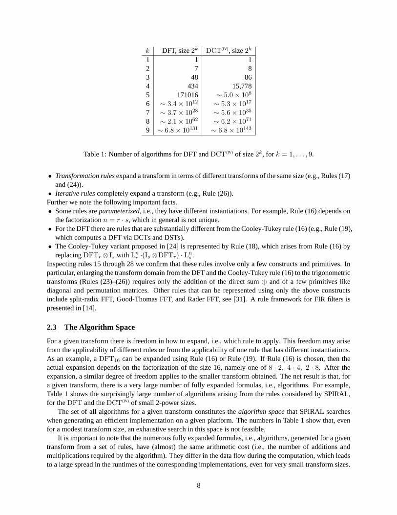
Table 1: Number of algorithms for DFT and DCT(IV) of size 2k, for k = 1, . . . , 9.

• Transformation rules expand a transform in terms of different transforms of the same size (e.g., Rules (17)and (24)).

• Iterative rules completely expand a transform (e.g., Rule (26)).Further we note the following important facts.• Some rules are parameterized, i.e., they have different instantiations. For example, Rule (16) depends on

the factorization n = r · s, which in general is not unique.• For the DFT there are rules that are substantially different from the Cooley-Tukey rule (16) (e.g., Rule (19),

which computes a DFT via DCTs and DSTs).• The Cooley-Tukey variant proposed in [24] is represented by Rule (18), which arises from Rule (16) by

replacing DFTr ⊗ Is with Lnr ·(Is⊗DFTr) · Ln

s .Inspecting rules 15 through 28 we confirm that these rules involve only a few constructs and primitives. Inparticular, enlarging the transform domain from the DFT and the Cooley-Tukey rule (16) to the trigonometrictransforms (Rules (23)–(26)) requires only the addition of the direct sum ⊕ and of a few primitives likediagonal and permutation matrices. Other rules that can be represented using only the above constructsinclude split-radix FFT, Good-Thomas FFT, and Rader FFT, see [31]. A rule framework for FIR filters ispresented in [14].

2.3 The Algorithm Space

For a given transform there is freedom in how to expand, i.e., which rule to apply. This freedom may arisefrom the applicability of different rules or from the applicability of one rule that has different instantiations.As an example, a DFT16 can be expanded using Rule (16) or Rule (19). If Rule (16) is chosen, then theactual expansion depends on the factorization of the size 16, namely one of 8 · 2, 4 · 4, 2 · 8. After theexpansion, a similar degree of freedom applies to the smaller transform obtained. The net result is that, fora given transform, there is a very large number of fully expanded formulas, i.e., algorithms. For example,Table 1 shows the surprisingly large number of algorithms arising from the rules considered by SPIRAL,for the DFT and the DCT(IV) of small 2-power sizes.

The set of all algorithms for a given transform constitutes the algorithm space that SPIRAL searcheswhen generating an efficient implementation on a given platform. The numbers in Table 1 show that, evenfor a modest transform size, an exhaustive search in this space is not feasible.

It is important to note that the numerous fully expanded formulas, i.e., algorithms, generated for a giventransform from a set of rules, have (almost) the same arithmetic cost (i.e., the number of additions andmultiplications required by the algorithm). They differ in the data flow during the computation, which leadsto a large spread in the runtimes of the corresponding implementations, even for very small transform sizes.

8

700 800 900 1000 1100 1200 1300 1400 15000

2

4

6

8

10

12

runtime [ns]400 500 600 700 800 900 10000

100

200

300

400

500

600

runtime [ns]

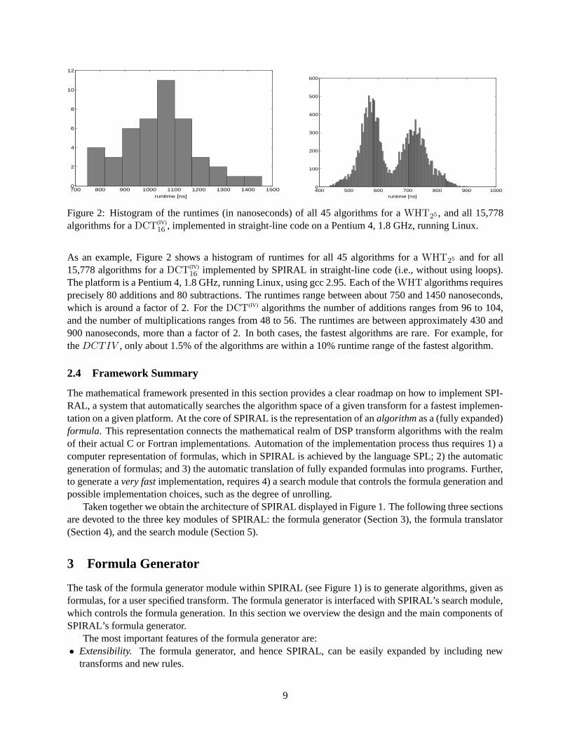
Figure 2: Histogram of the runtimes (in nanoseconds) of all 45 algorithms for a WHT25 , and all 15,778algorithms for a DCT(IV)

16 , implemented in straight-line code on a Pentium 4, 1.8 GHz, running Linux.

As an example, Figure 2 shows a histogram of runtimes for all 45 algorithms for a WHT25 and for all15,778 algorithms for a DCT(IV)

16 implemented by SPIRAL in straight-line code (i.e., without using loops).The platform is a Pentium 4, 1.8 GHz, running Linux, using gcc 2.95. Each of the WHT algorithms requiresprecisely 80 additions and 80 subtractions. The runtimes range between about 750 and 1450 nanoseconds,which is around a factor of 2. For the DCT(IV) algorithms the number of additions ranges from 96 to 104,and the number of multiplications ranges from 48 to 56. The runtimes are between approximately 430 and900 nanoseconds, more than a factor of 2. In both cases, the fastest algorithms are rare. For example, forthe DCTIV , only about 1.5% of the algorithms are within a 10% runtime range of the fastest algorithm.

2.4 Framework Summary

The mathematical framework presented in this section provides a clear roadmap on how to implement SPI-RAL, a system that automatically searches the algorithm space of a given transform for a fastest implemen-tation on a given platform. At the core of SPIRAL is the representation of an algorithm as a (fully expanded)formula. This representation connects the mathematical realm of DSP transform algorithms with the realmof their actual C or Fortran implementations. Automation of the implementation process thus requires 1) acomputer representation of formulas, which in SPIRAL is achieved by the language SPL; 2) the automaticgeneration of formulas; and 3) the automatic translation of fully expanded formulas into programs. Further,to generate a very fast implementation, requires 4) a search module that controls the formula generation andpossible implementation choices, such as the degree of unrolling.

Taken together we obtain the architecture of SPIRAL displayed in Figure 1. The following three sectionsare devoted to the three key modules of SPIRAL: the formula generator (Section 3), the formula translator(Section 4), and the search module (Section 5).

3 Formula Generator

The task of the formula generator module within SPIRAL (see Figure 1) is to generate algorithms, given asformulas, for a user specified transform. The formula generator is interfaced with SPIRAL’s search module,which controls the formula generation. In this section we overview the design and the main components ofSPIRAL’s formula generator.

The most important features of the formula generator are:• Extensibility. The formula generator, and hence SPIRAL, can be easily expanded by including new

transforms and new rules.

9

DFT2 DFT2

DFT4 DFT2

DFT8

���HHH

���HHH

↔((

(F2⊗ I2) · T42 · (I2⊗F2) · L4

2

)⊗ I2

)

·T82 ·(I4⊗F2) · L8

4

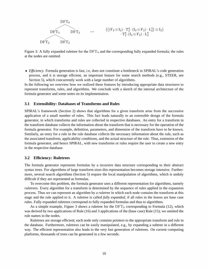
Figure 3: A fully expanded ruletree for the DFT8 and the corresponding fully expanded formula; the rulesat the nodes are omitted.

• Efficiency. Formula generation is fast, i.e, does not constitute a bottleneck in SPIRAL’s code generationprocess, and it is storage efficient, an important feature for some search methods (e.g., STEER, seeSection 5), which concurrently work with a large number of algorithms.

In the following we overview how we realized these features by introducing appropriate data structures torepresent transforms, rules, and algorithms. We conclude with a sketch of the internal architecture of theformula generator and some notes on its implementation.

3.1 Extensibility: Databases of Transforms and Rules

SPIRAL’s framework (Section 2) shows that algorithms for a given transform arise from the successiveapplication of a small number of rules. This fact leads naturally to an extensible design of the formulagenerator, in which transforms and rules are collected in respective databases. An entry for a transform inthe transform database collects the information about the transform that is necessary for the operation of theformula generator. For example, definition, parameters, and dimension of the transform have to be known.Similarly, an entry for a rule in the rule database collects the necessary information about the rule, such asthe associated transform, applicability conditions, and the actual structure of the rule. Thus, extension of theformula generator, and hence SPIRAL, with new transforms or rules require the user to create a new entryin the respective database.

3.2 Efficiency: Ruletrees

The formula generator represents formulas by a recursive data structure corresponding to their abstractsyntax trees. For algorithms of large transform sizes this representation becomes storage intensive. Further-more, several search algorithms (Section 5) require the local manipulation of algorithms, which is undulydifficult if they are represented as formulas.

To overcome this problem, the formula generator uses a different representation for algorithms, namelyruletrees. Every algorithm for a transform is determined by the sequence of rules applied in the expansionprocess. Thus we can represent an algorithm by a ruletree in which each node contains the transform at thisstage and the rule applied to it. A ruletree is called fully expanded, if all rules in the leaves are base caserules. Fully expanded ruletrees correspond to fully expanded formulas and thus to algorithms.

As a simple example, Figure 3 shows a ruletree for the DFT8 corresponding to Formula (12), whichwas derived by two applications of Rule (16) and 3 applications of the (base case) Rule (15); we omitted therule names in the nodes.

Ruletrees are storage efficient; each node only contains pointers to the appropriate transform and rule inthe database. Furthermore, ruletrees can be easily manipulated, e.g., by expanding a subtree in a differentway. The efficient representation also leads to the very fast generation of ruletrees. On current computingplatforms, thousands of trees can be generated in a few seconds.

10

For

mul

aG

ener

ator

transforms -

rules

?

recursiveapplication

ruletrees - formulas

Search Engine�controls

-export

�runtime

FormulaTranslator

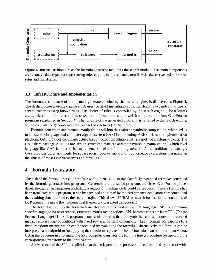
Figure 4: Internal architecture of the formula generator including the search module. The main componentsare recursive data types for representing ruletrees and formulas, and extensible databases (dashed boxes) forrules and transforms.

3.3 Infrastructure and Implementation

The internal architecture of the formula generator, including the search engine, is displayed in Figure 4.The dashed boxes indicate databases. A user specified instantiation of a transform is expanded into one orseveral ruletrees using known rules. The choice of rules is controlled by the search engine. The ruletreesare translated into formulas and exported to the formula translator, which compiles them into C or Fortranprograms (explained in Section 4). The runtime of the generated programs is returned to the search engine,which controls the generation of the next set of ruletrees (see Section 5).

Formula generation and formula manipulation fall into the realm of symbolic computation, which led usto choose the language and computer algebra system GAP [12], including AREP [5], as an implementationplatform. GAP provides the infrastructure for symbolic computation with a variety of algebraic objects. TheGAP share package AREP is focused on structured matrices and their symbolic manipulation. A high levellanguage like GAP facilitates the implementation of the formula generator. As an additional advantage,GAP provides exact arithmetic for square roots, roots of unity, and trigonometric expressions that make upthe entries of most DSP transforms and formulas.

4 Formula Translator

The task of the formula translator module within SPIRAL is to translate fully expanded formulas generatedby the formula generator into programs. Currently, the translated programs are either C or Fortran proce-dures, though other languages including assembly or machine code could be produced. Once a formula hasbeen translated into a program, it can be executed and timed by the performance evaluation component andthe resulting time returned to the search engine. This allows SPIRAL to search for fast implementations ofDSP transforms using the mathematical framework presented in Section 2.

The formulas input to the formula translator are represented in the SPL language. SPL is a domain-specific language for representing structured matrix factorizations. SPL borrows concepts from TPL (TensorProduct Language) [1]. SPL programs consist of formulas that are symbolic representations of structuredmatrix factorizations of matrices with fixed row and column dimensions. Each formula corresponds to afixed transform matrix, which can be obtained by evaluating the formula. Alternatively, the formula can beinterpreted as an algorithm for applying the transform represented by the formula to an arbitrary input vector.Using the structure in a formula, the SPL compiler translates the formula into a procedure for applying thecorresponding transform to the input vector.

A key feature of the SPL compiler is that the code generation process can be controlled by the user with-

11

out modifying the compiler. This is done through the use of compiler directives and a template mechanismcalled meta-SPL. Meta-SPL allows SPIRAL, in addition to searching through the space of algorithms, tosearch through the space of possible implementations for a given formula. A key research question is to de-termine which optimizations should be performed by default by the SPL compiler and which optimizationsshould be controlled by the search engine in SPIRAL. Some optimizations, such as common subexpressionelimination, are always applied; however, other potential optimizations, such as loop unrolling, for whichit is not clear when and to what level to apply, are implementation parameters for the search engine to ex-plore. It is worth noting that it is necessary for the SPL compiler to apply standard compiler optimizationssuch as common subexpression elimination, rather leaving them to the backend C or Fortran compiler, sincethese compilers typically do not fully utilize these optimizations on the type of code produced by the SPLcompiler [38].

The SPL representation of algorithms around which SPIRAL is built is very different from FFTW’scodelet generator, which represents algorithms as a collection of arithmetic expression trees for each output,which then is translated into a dataflow graph using various optimizations [10]. In both cases, the repre-sentation is restricted to a limited class of programs corresponding to linear computations of a fixed size,which have simplifying properties such as no side-effects and no conditionals. This opens the possibilityfor domain-specific optimizations. Advantages of the SPL representation of algorithms as generated by theformula generator include the following: 1) Formula generation is separated from formula translation andboth the formula generator and formula translator can be developed, maintained, and used independently. Inparticular, the formula generator can be used by DSP experts to include new transforms and algorithms. SPLprovides a natural language to transfer information between the two components. 2) The representation isconcise. The arithmetic expression tree representation used in FFTW expresses each output as linear func-tion of all n inputs and thus grows roughly as O(n2 log(n)), which restricts its application to small transformsizes (which, of course, is the intended scope and sufficient in FFTW). 3) High-level mathematical knowl-edge is maintained, and this knowledge can be used to obtain optimizations and program transformationsnot available using standard compiler techniques. This is crucial, for example, for short-vector code gen-eration (Section 4.4). 4) The mathematical nature of SPL allows other programs, in our case the formulagenerator, to easily manipulate and derive alternate programs. Moreover, algorithms are expressed naturallyusing the underlying mathematics. 5) SPL provides hooks that allow alternative code generation schemesand optimizations to be controlled and searched externally without modifying the compiler.

In the following three subsections we describe SPL, meta-SPL, and the SPL compiler, respectively. Anoverview of the language and compiler will be given, and several examples will be provided, illustratingthe syntax of the language and the translation process used by the compiler. Additional information maybe found in [38] and [37]. We conclude with a brief overview of an extension to the SPL compiler thatgenerates short vector code for last generation platforms that feature SIMD (single-instruction multiple-data) instruction set extensions.

4.1 SPL

In this section we describe the constructs and syntax of the SPL language. Syntax is described informallyguided by the natural mathematical interpretation. A more formal treatment along with a BNF grammaris available in [37]. In the next section we describe meta-SPL, a meta-language that is used to define thesemantics of SPL and allows the language to be extended.

SPL programs consist of the following: 1) SPL formulas, representing fully expanded formulas in thesense of Section 2.1; 2) constant expressions for entries appearing in formulas; 3) define statements forassigning names to formulas or constant expressions; and 4) compiler directives and type declarations. Eachformula corresponds to a factorization of a real or complex matrix of a fixed size. The size is determinedfrom the formula using meta-SPL, and the type is specified as real or complex. Meta-SPL is also used

12

to define the symbols occurring in formulas. Rather than constructing matrices, meta-SPL is used by thecompiler to generate a procedure for applying the transform (as represented by a formula) to an input vectorof the given size and type.

Constant expressions. The elements of a matrix can be real or complex numbers. Complex numbersa+b√−1 are represented by the pair of real numbers (a, b). In SPL, these numbers can be specified as scalar

constant expressions, which may contain function invocations and symbolic constants like pi. For example,12, 1.23, 5*pi, sqrt(5), and (cos(2*pi/3.0),sin(2*pi/3)) are valid scalar SPL expressions. Allconstant scalar expressions are evaluated at compile-time.

SPL formulas. SPL formulas are built from general matrix constructions, parameterized symbols de-noting families of special matrices, and matrix operations such as matrix composition, direct sum, and thetensor product. Each construction has a list of arguments that uniquely determine the corresponding matrix.The distinction between the different constructions is mainly conceptual; however it also corresponds todifferent argument types.

SPL uses a prefix notation similar to Lisp to represent formulas. The following lists example construc-tions that are provided from each category. However, it is possible to define new general matrix construc-tions, parameterized symbols, and matrix operations using meta-SPL.

General matrix constructions. Let aij denote an SPL constant and ik, jk, and σk denote positiveintegers. Examples include the following.• (matrix (a11 ... a1n) ... (am1 ... amn)) - the m× n matrix [aij ]1≤i≤m, 1≤j≤n.• (sparse (i1 j1 ai1j1) ... (it jt aitjt)) - the m × n matrix where m = max(i1, . . . , it), n =

max(j1, . . . , jt) and the non-zero entries are aikjkfor k = 1, . . . , t.

• (diagonal (a1 ... an)) - the n× n diagonal matrix diag(a1, . . . , an).• (permutation (σ1 ... σn)) - the n× n permutation matrix: k 7→ σk, for k = 1, . . . , n.

Parameterized Symbols. Parameterized symbols represent families of matrices parameterized by inte-gers. Examples include the following.• (I n) - the n× n identity matrix In.• (F n) - the n× n DFT matrix Fn.• (L n s) - the n× n stride permutation matrix Ln

s , where s|n.• (T n s) - the n× n twiddle matrix Tn

s , where s|n.Matrix operations. Matrix operations take a list of SPL formulas, i.e. matrices, and construct an-

other matrix. In the following examples, A and Ai are arbitrary SPL formulas and P is an SPL formulacorresponding to a permutation matrix.• (compose A1 ... At) - the matrix product A1 · · ·At.• (direct-sum A1 ... At) - the direct sum A1 ⊕ · · · ⊕At.• (tensor A1 ... At) - the tensor product A1 ⊗ · · · ⊗At.• (conjugate A P) - the matrix conjugation AP = P−1 ·A · P , where P is a permutation.

Define Statements are provided for assigning names to formulas or constant expressions. They providea short-hand for entering subformulas or constants in formulas.• (define name formula)

• (define name constant-expression)

Compiler Directives. There are two types of compiler directives. The first type is used to specify thematrix type, and the second type is used to influence the code produced by the compiler.• #datatype REAL | COMPLEX - set the type of the input and output vectors.• #subname name - name of the procedure produced by the compiler for the code that follows.• #codetype REAL | COMPLEX - if the datatype is complex, indicate whether complex are real variables

will be used to implement complex arithmetic in the generated code.• #unroll ON | OFF - if ON generate straight-line code and if OFF generate loop code.

13

#datatype COMPLEX #datatype REAL

#codetype REAL #unroll ON

#unroll ON #subname DCT2_4

(define F4 (compose

(compose (permutation (1 3 2 4))

(tensor (F 2) (I 2)) (direct_sum

(T 4 2) (compose (diagonal (1 sqrt(1/2))) (F 2))

(tensor (I 2) (F 2) (matrix

(L 4 2))) ( cos(13*pi/8) sin(13*pi/8))

#subname F_8 (-sin(13*pi/8) cos(13*pi/8))

#unroll OFF )

(compose )

(tensor F4 (I 2)) (permutation (1 3 2 4))

(T 8 2) (tensor (I 2) (F 2))

(tensor (I 4) (F 2)) (permutation (1 4 2 3))

(L 8 4)) )

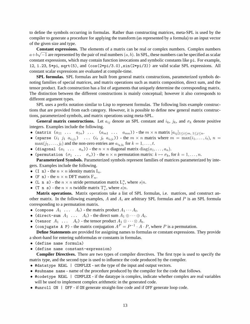
Figure 5: SPL expressions for DFT8 and DCT(II)4 .

Figure 5 shows SPL expressions for the fully expanded formulas for the transforms DFT8 and DCT(II)4 ,

corresponding to (12) and (11), respectively. These examples use all of the components of SPL includingparameterized symbols, general matrix constructions, matrix operations, constant expressions, define state-ments, and compiler directives. These SPL formulas will be translated into C or Fortran procedures with thenames F 8 and DCT2 4 respectively. The procedure F 8 has a complex input and output of size 8 and usesa mixture of loop and straight-line code. Complex arithmetic is explicitly computed with real arithmeticexpressions. The procedure DCT2 4 has a real input and output of size 4 and is implemented in straight-linecode.

4.2 Meta-SPL

The semantics of SPL programs are defined in meta-SPL using a template mechanism. Templates tell thecompiler how to generate code for the various symbols that occur in SPL formulas. In this way, templatesare used to define general matrix constructions, parameterized symbols and matrix operations, includingthose built-in and those newly created by the user. They also provide a mechanism to compute the inputand output dimensions of the matrices corresponding to a formula. In addition to templates, meta-SPL candefine functions (scalar, vector, and matrix) that can be used in template definitions. Finally, statements areprovided to inform the parser of the symbols that are defined by templates.

Symbol definition, intrinsic functions, and templates. Meta-SPL provides the following directivesto introduce parameterized matrices, general matrix constructions, matrix operators, intrinsic functions andtemplates.• (primitive name shape) - introduce new parameterized symbol.• (direct name size-rule) - introduce a new general matrix construction.• (operation name size-rule) - introduce new matrix operation.• (function name <arguments> <dimension> expression) - define an intrinsic function.• (template formula [condition] (i-code-list)) - define a template.The parameters shape and size-rule specify how the row and column dimensions of the representedmatrix are computed.

14

(template (T n s) ;; ---- n and s are integer parameters

[n >= 1 && s >= 1 && n%s == 0]

( coldim = n

rowdim = n

for i=0,...,n-1

y(i) = w(n,i*s) * x(i)

end ) )

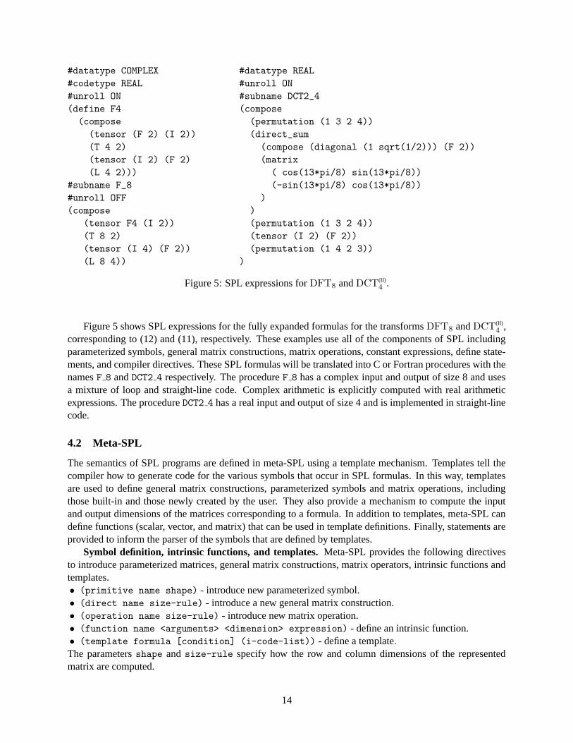
Figure 6: Template for (T n s).

A template contains a pattern followed by an optional guard condition and a code sequence using an in-termediate code representation called i-code. When the SPL compiler encounters an expression that matchesthe pattern and satisfies the guard condition, it inserts the corresponding i-code into the translated program,where the parameters are replaced by the values in the matched expression.

Templates use the convention that the input and output vectors are always referred to by the names x andy and have sizes given by coldim and rowdim. Intermediate code can refer to x, y, the input parameters,and temporary variables. The code consists of a sequence of two operand assignments and conditionals arenot allowed. Loops are allowed; however, the number of iterations, once the template is instantiated willalways be constant.

The following examples illustrate how templates are used to define parameterized symbols and matrixoperations. A detailed description of templates is provided in [37]. Note that the syntax used here is slightlysimplified to allow for a more accessible presentation. Also row and column dimensions are computedexplicitly rather than relying on size and shape rules.

Figure 6 shows the template definition for the parameterized symbol (T n s). The pattern (T n s)willmatch any SPL expression containing the symbol T in the first position followed by two integer parameters.The guard condition specifies that the two integer parameters are positive and the second parameter dividesthe first. The resulting code multiplies the input vector x by constants produced from intrinsic function calls:w(n, k) = ωk

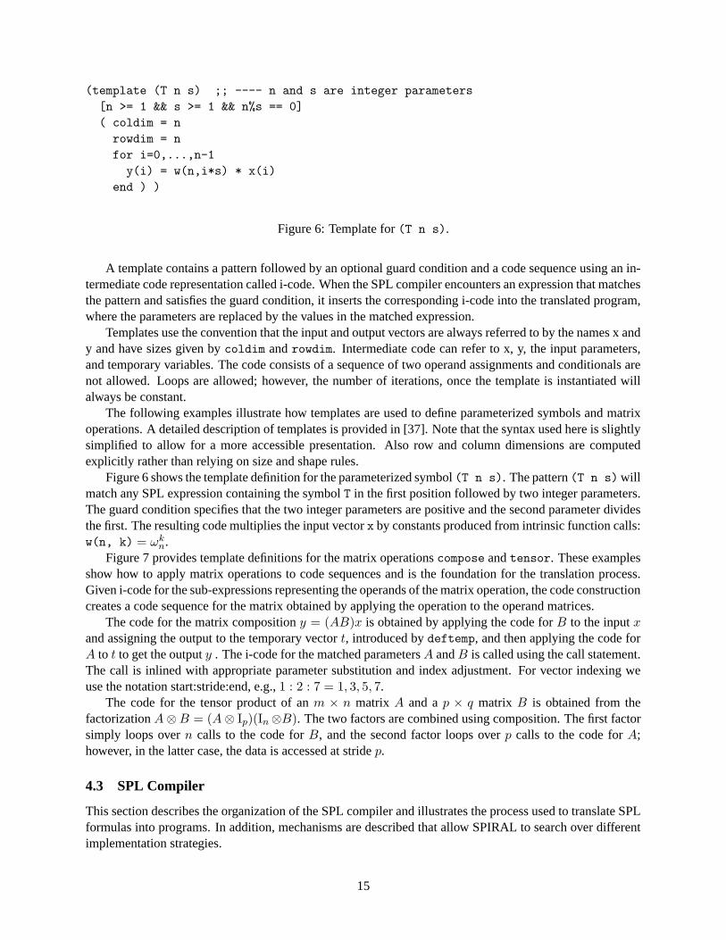
n.Figure 7 provides template definitions for the matrix operations compose and tensor. These examples

show how to apply matrix operations to code sequences and is the foundation for the translation process.Given i-code for the sub-expressions representing the operands of the matrix operation, the code constructioncreates a code sequence for the matrix obtained by applying the operation to the operand matrices.

The code for the matrix composition y = (AB)x is obtained by applying the code for B to the input xand assigning the output to the temporary vector t, introduced by deftemp, and then applying the code forA to t to get the output y . The i-code for the matched parameters A and B is called using the call statement.The call is inlined with appropriate parameter substitution and index adjustment. For vector indexing weuse the notation start:stride:end, e.g., 1 : 2 : 7 = 1, 3, 5, 7.

The code for the tensor product of an m × n matrix A and a p × q matrix B is obtained from thefactorization A⊗B = (A⊗ Ip)(In⊗B). The two factors are combined using composition. The first factorsimply loops over n calls to the code for B, and the second factor loops over p calls to the code for A;however, in the latter case, the data is accessed at stride p.

4.3 SPL Compiler

This section describes the organization of the SPL compiler and illustrates the process used to translate SPLformulas into programs. In addition, mechanisms are described that allow SPIRAL to search over differentimplementation strategies.

15

(template (compose A B) ; y = (A B) x = A(B(x)).

( deftemp t(B.rowdim)

coldim = A.rowdim

rowdim = B.coldim

t(0:1:B.rowdim-1) = call B(x(0:1:B.coldim-1))

y(0:1:A.rowdim-1) = call A(t(0:1:B.rowdim-1)) ) )

(template (tensor A B) ; y = (A tensor B) x

( rowdim = A.rowdim * B.rowdim

coldim = A.coldim * B.coldim

deftemp t(A.coldim*B.rowdim)

for i=0:A.coldim-1

t(i*B.rowdim:1:(i+1)*B.rowdim-1) =

call B(x(i*B.coldim:1:(i+1)*B.coldim-1));

end

for j=0:B.rowdim-1

y(j*A.rowdim:B.rowdim:(j+1)*A.rowdim-1) =

call A(t(j*A.coldim:B.rowdim:(j+1)*A.coldim -1 )

end ) )

Figure 7: Templates for compose and tensor.

The SPL compiler translates an SPL formula (matrix factorization) into an efficient program (currentlyin C or Fortran) to compute the matrix-vector product of the matrix given by the SPL formula. Transla-tion proceeds by applying various transformations, corresponding to the algebraic operators in SPL, to codesegments starting with code for the matrices occurring in the SPL formula. The code segments and transfor-mations are defined by the template mechanism in meta-SPL discussed in the previous section. Meta-SPLalso provides a mechanism to control the optimization and code generation strategies used by the compiler.

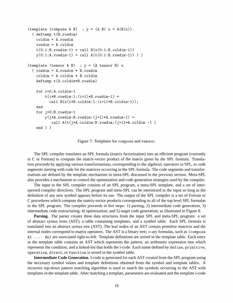
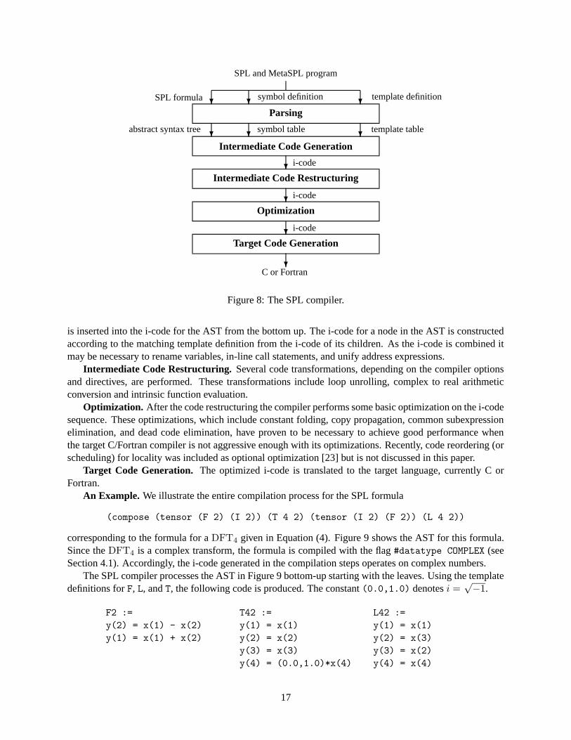
The input to the SPL compiler consists of an SPL program, a meta-SPL template, and a set of inter-spersed compiler directives. The SPL program and meta-SPL can be intermixed in the input so long as thedefinition of any new symbol appears before its use. The output of the SPL compiler is a set of Fortran orC procedures which compute the matrix-vector products corresponding to all of the top level SPL formulasin the SPL program. The compiler proceeds in five steps: 1) parsing; 2) intermediate code generation; 3)intermediate code restructuring; 4) optimization; and 5) target code generation; as illustrated in Figure 8.

Parsing. The parser creates three data structures from the input SPL and meta-SPL program: a setof abstract syntax trees (AST), a table containing templates, and a symbol table. Each SPL formula istranslated into an abstract syntax tree (AST). The leaf nodes of an AST contain primitive matrices and theinternal nodes correspond to matrix operators. The AST is a binary tree; n-ary formulas, such as (composeA1 ... An) are associated right-to-left. Template definitions are stored in the template table. Each entryin the template table contains an AST which represents the pattern, an arithmetic expression tree whichrepresents the condition, and a linked-list that holds the i-code. Each name defined by define, primitive,operation, direct, or function is stored in the symbol table.

Intermediate Code Generation. I-code is generated for each AST created from the SPL program usingthe necessary symbol values and template definitions obtained from the symbol and template tables. Arecursive top-down pattern matching algorithm is used to match the symbols occurring in the AST withtemplates in the template table. After matching a template, parameters are evaluated and the template i-code

16

C or Fortran?

Target Code Generation?i-code

Optimization?i-code

Intermediate Code Restructuring?i-code

Intermediate Code Generation?abstract syntax tree ?symbol table ? template table

Parsing?SPL formula ?symbol definition ? template definition

SPL and MetaSPL program

Figure 8: The SPL compiler.

is inserted into the i-code for the AST from the bottom up. The i-code for a node in the AST is constructedaccording to the matching template definition from the i-code of its children. As the i-code is combined itmay be necessary to rename variables, in-line call statements, and unify address expressions.

Intermediate Code Restructuring. Several code transformations, depending on the compiler optionsand directives, are performed. These transformations include loop unrolling, complex to real arithmeticconversion and intrinsic function evaluation.

Optimization. After the code restructuring the compiler performs some basic optimization on the i-codesequence. These optimizations, which include constant folding, copy propagation, common subexpressionelimination, and dead code elimination, have proven to be necessary to achieve good performance whenthe target C/Fortran compiler is not aggressive enough with its optimizations. Recently, code reordering (orscheduling) for locality was included as optional optimization [23] but is not discussed in this paper.

Target Code Generation. The optimized i-code is translated to the target language, currently C orFortran.

An Example. We illustrate the entire compilation process for the SPL formula

(compose (tensor (F 2) (I 2)) (T 4 2) (tensor (I 2) (F 2)) (L 4 2))

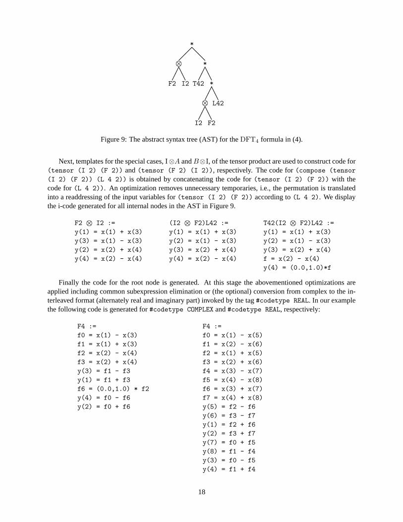
corresponding to the formula for a DFT4 given in Equation (4). Figure 9 shows the AST for this formula.Since the DFT4 is a complex transform, the formula is compiled with the flag #datatype COMPLEX (seeSection 4.1). Accordingly, the i-code generated in the compilation steps operates on complex numbers.

The SPL compiler processes the AST in Figure 9 bottom-up starting with the leaves. Using the templatedefinitions for F, L, and T, the following code is produced. The constant (0.0,1.0) denotes i =

√−1.

F2 :=

y(2) = x(1) - x(2)

y(1) = x(1) + x(2)

T42 :=

y(1) = x(1)

y(2) = x(2)

y(3) = x(3)

y(4) = (0.0,1.0)*x(4)

L42 :=

y(1) = x(1)

y(2) = x(3)

y(3) = x(2)

y(4) = x(4)

17

F2 I2 T42 *

⊗ *�

�AA

��

AA

��

@@*

⊗ L42��

AA

��

AA

I2 F2

Figure 9: The abstract syntax tree (AST) for the DFT4 formula in (4).

Next, templates for the special cases, I⊗A and B⊗I, of the tensor product are used to construct code for(tensor (I 2) (F 2)) and (tensor (F 2) (I 2)), respectively. The code for (compose (tensor

(I 2) (F 2)) (L 4 2)) is obtained by concatenating the code for (tensor (I 2) (F 2)) with thecode for (L 4 2)). An optimization removes unnecessary temporaries, i.e., the permutation is translatedinto a readdressing of the input variables for (tensor (I 2) (F 2)) according to (L 4 2). We displaythe i-code generated for all internal nodes in the AST in Figure 9.

F2 ⊗ I2 :=

y(1) = x(1) + x(3)

y(3) = x(1) - x(3)

y(2) = x(2) + x(4)

y(4) = x(2) - x(4)

(I2 ⊗ F2)L42 :=

y(1) = x(1) + x(3)

y(2) = x(1) - x(3)

y(3) = x(2) + x(4)

y(4) = x(2) - x(4)

T42(I2 ⊗ F2)L42 :=

y(1) = x(1) + x(3)

y(2) = x(1) - x(3)

y(3) = x(2) + x(4)

f = x(2) - x(4)

y(4) = (0.0,1.0)*f

Finally the code for the root node is generated. At this stage the abovementioned optimizations areapplied including common subexpression elimination or (the optional) conversion from complex to the in-terleaved format (alternately real and imaginary part) invoked by the tag #codetype REAL. In our examplethe following code is generated for #codetype COMPLEX and #codetype REAL, respectively:

F4 :=

f0 = x(1) - x(3)

f1 = x(1) + x(3)

f2 = x(2) - x(4)

f3 = x(2) + x(4)

y(3) = f1 - f3

y(1) = f1 + f3

f6 = (0.0,1.0) * f2

y(4) = f0 - f6

y(2) = f0 + f6

F4 :=

f0 = x(1) - x(5)

f1 = x(2) - x(6)

f2 = x(1) + x(5)

f3 = x(2) + x(6)

f4 = x(3) - x(7)

f5 = x(4) - x(8)

f6 = x(3) + x(7)

f7 = x(4) + x(8)

y(5) = f2 - f6

y(6) = f3 - f7

y(1) = f2 + f6

y(2) = f3 + f7

y(7) = f0 + f5

y(8) = f1 - f4

y(3) = f0 - f5

y(4) = f1 + f4

18

Loop Code. The code generated in the previous example consists entirely of straight-line code. TheSPL compiler can be instructed to generate loop code by using templates with loops such as those for thetwiddle symbol and the tensor product. Using these templates, the SPL compiler translates the expression(compose (F 2) (I 4)) (T 8 4)) into the following Fortran code.

do i0 = 0, 7

t0(i0+1) = T8_4(i0+1) * x(i0+1)

end do

do i0 = 0, 3

y(i0+5) = t0(i0+1) - t0(i0+5)

y(i0+1) = t0(i0+1) + t0(i0+5)

end do

Since loops are used, constants must be placed in an array so that they can be indexed by the loop variable.Initialization code is produced by the compiler to initialize arrays containing constants. In this example, theconstants from T8

4 are placed in the array T8 4.Observe that the data must be accessed twice: once to multiply by the twiddle matrix and once to

compute F2⊗ I4. By introducing an additional template that matches the expression that combines F2⊗ I4and the preceding twiddle matrix, the computation can be performed in one pass.

do i0 = 0, 3

r1 = 4 + i0

f0 = T8_4(r1+1) * x(i0+5)

y(i0+5) = x(i0+1) - f0

y(i0+1) = x(i0+1) + f0

end do

This example shows how the user can control the compilation process through the use of templates.In order to generate efficient code it is often necessary to combine loop code and straight-line code.

This can be accomplished through the use of loop unrolling. After matching a template pattern with loopsthe instantiated code has constant loop bounds. The compiler may be directed to unroll the loops, fully orpartially to reduce loop overhead and increase the number of choices in instruction scheduling. When theloops are fully unrolled, not only is the loop overhead eliminated but it also becomes possible to substitutescalar expressions for array elements. The use of scalar variables tends to improve the quality of the codegenerated by Fortran and C compilers which are usually unable to analyze codes containing array subscripts.The down side of unrolling is the increase in code size.

In SPL, the degree of unrolling can be specified for the whole program or for a single formula. Forexample, the compiler option -B32 instructs the compiler to fully unroll all loops in those sub-formulaswhose input vector is smaller than or equal to 32. Individual formulas can be unrolled through the use of the#unroll directive. For example

#unroll on

(define I2F2 (tensor (I 2) (F 2)))

#unroll off

(tensor (I 32) I2F2)

will be translated into the following code.

do i0 = 0, 31

y(4*i0+2) = x(4*i0+1) - x(4*i0+2)

19

y(4*i0+1) = x(4*i0+1) + x(4*i0+2)

y(4*i0+4) = x(4*i0+3) - x(4*i0+4)

y(4*i0+3) = x(4*i0+3) + x(4*i0+4)

end do

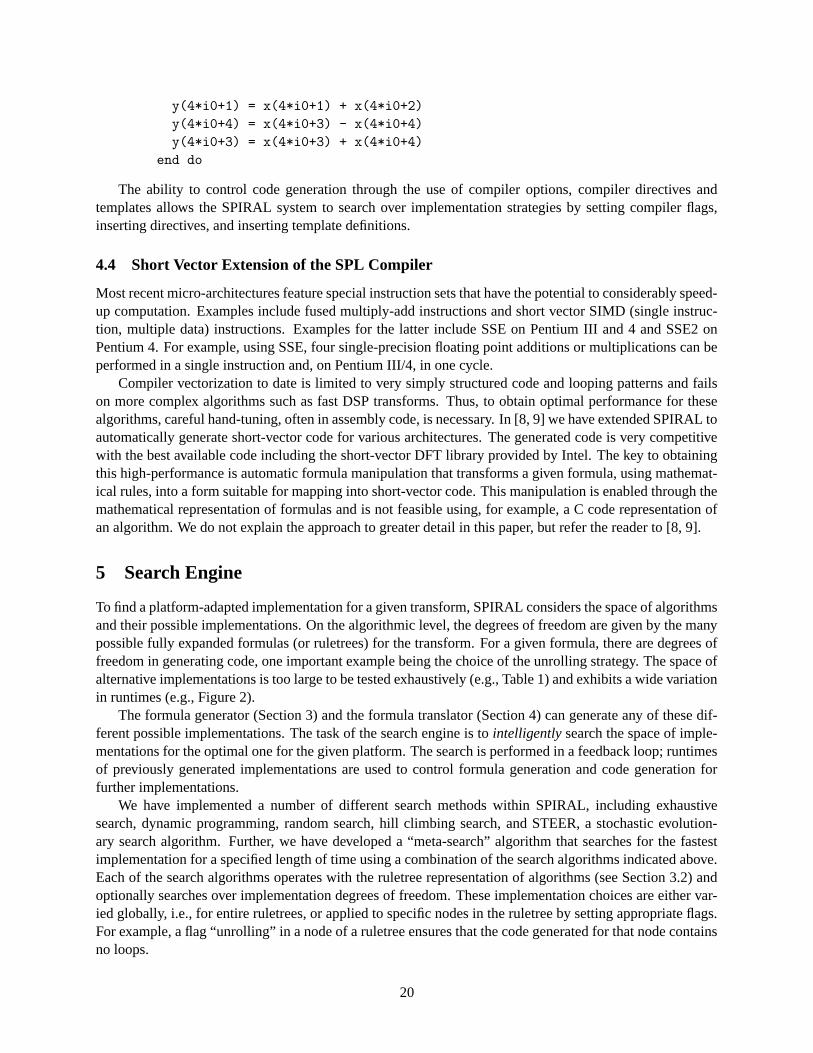
The ability to control code generation through the use of compiler options, compiler directives andtemplates allows the SPIRAL system to search over implementation strategies by setting compiler flags,inserting directives, and inserting template definitions.

4.4 Short Vector Extension of the SPL Compiler

Most recent micro-architectures feature special instruction sets that have the potential to considerably speed-up computation. Examples include fused multiply-add instructions and short vector SIMD (single instruc-tion, multiple data) instructions. Examples for the latter include SSE on Pentium III and 4 and SSE2 onPentium 4. For example, using SSE, four single-precision floating point additions or multiplications can beperformed in a single instruction and, on Pentium III/4, in one cycle.

Compiler vectorization to date is limited to very simply structured code and looping patterns and failson more complex algorithms such as fast DSP transforms. Thus, to obtain optimal performance for thesealgorithms, careful hand-tuning, often in assembly code, is necessary. In [8, 9] we have extended SPIRAL toautomatically generate short-vector code for various architectures. The generated code is very competitivewith the best available code including the short-vector DFT library provided by Intel. The key to obtainingthis high-performance is automatic formula manipulation that transforms a given formula, using mathemat-ical rules, into a form suitable for mapping into short-vector code. This manipulation is enabled through themathematical representation of formulas and is not feasible using, for example, a C code representation ofan algorithm. We do not explain the approach to greater detail in this paper, but refer the reader to [8, 9].

5 Search Engine

To find a platform-adapted implementation for a given transform, SPIRAL considers the space of algorithmsand their possible implementations. On the algorithmic level, the degrees of freedom are given by the manypossible fully expanded formulas (or ruletrees) for the transform. For a given formula, there are degrees offreedom in generating code, one important example being the choice of the unrolling strategy. The space ofalternative implementations is too large to be tested exhaustively (e.g., Table 1) and exhibits a wide variationin runtimes (e.g., Figure 2).

The formula generator (Section 3) and the formula translator (Section 4) can generate any of these dif-ferent possible implementations. The task of the search engine is to intelligently search the space of imple-mentations for the optimal one for the given platform. The search is performed in a feedback loop; runtimesof previously generated implementations are used to control formula generation and code generation forfurther implementations.

We have implemented a number of different search methods within SPIRAL, including exhaustivesearch, dynamic programming, random search, hill climbing search, and STEER, a stochastic evolution-ary search algorithm. Further, we have developed a “meta-search” algorithm that searches for the fastestimplementation for a specified length of time using a combination of the search algorithms indicated above.Each of the search algorithms operates with the ruletree representation of algorithms (see Section 3.2) andoptionally searches over implementation degrees of freedom. These implementation choices are either var-ied globally, i.e., for entire ruletrees, or applied to specific nodes in the ruletree by setting appropriate flags.For example, a flag “unrolling” in a node of a ruletree ensures that the code generated for that node containsno loops.

20

The different search algorithms are described in more detail below.

5.1 Exhaustive Search

Exhaustive search is straightforward. It generates all the possible implementations for a given transform andtimes each one to determine the fastest one. This search method is only feasible for very small transformsizes, as the number of possible algorithms for most transforms grows exponentially with the transformsize. For example, Table 1 shows that exhaustive search becomes impractical for DFTs of size 26 and forDCT(IV)’s of size 25.

5.2 Dynamic Programming

Dynamic programming (DP) is a common approach to search in this type of domain [18, 11, 16, 28]. DPrecursively builds a table of the best ruletrees found for each transform. A given transform is expanded onceusing all applicable rules. The ruletrees, i.e., expansions, of the obtained children are looked up in the table.If a ruletree is not present, then DP is called recursively on this child. Finally, the table is updated with thefastest ruletree of the given transform. DP usually times fewer ruletrees than the other search methods.

Dynamic programming makes the following assumption:

Dynamic Programming Assumption: The best ruletree for a transform is also the best way tosplit that transform in a larger ruletree.

This assumption does not hold in general; the performance of a ruletree varies greatly depending on itsposition in a larger ruletree due to the pattern of data flow and the internal state of the given machine. Inpractice, though, DP usually finds reasonably fast formulas. A variant of DP considered by SPIRAL keepstrack of the n best ruletrees found at each level, thus relaxing the DP assumption.

5.3 Random Search

Random search generates a number of random ruletrees and chooses the fastest. Note that it is a nontrivialproblem to uniformly draw ruletrees from the space of all possibilities, i.e., algorithms. Thus, in the currentimplementation, a random ruletree is generated by choosing (uniformly) a random rule in each step of theexpansion of the given transform.

Random search has the advantage that it times as few or as many formulas as the user desires, but leadsto poor results if the fast ruletrees are scarce.

5.4 STEER

STEER (Split Tree Evolution for Efficient Runtimes) uses a stochastic, evolutionary search approach [29,30]. STEER is similar to genetic algorithms [15], except that, instead of using a bit vector representa-tion, it uses ruletrees as its representation. Unlike random search, STEER uses evolutionary operators tostochastically guide its search toward more promising portions of the space of formulas.

Given a transform and size of interest, STEER proceeds as follows:1. Randomly generate a population P of legal ruletrees of the given transform and size.2. For each ruletree in P , obtain its running time.3. Let Pfastest be the set of the b fastest trees in P .4. Randomly select from P , favoring faster trees, to generate a new population Pnew.5. Cross-over c random pairs of trees in Pnew.6. Mutate m random trees in Pnew.

21

7. Let P ← Pfastest ∪ Pnew.8. Repeat step 2 and following.

All selections are performed with replacement so that Pnew may contain multiple copies of the same tree.Since timing ruletrees is expensive, runtimes are cached and only new ruletrees in P at step 2 are actuallytimed.

During this process, the ruletrees may not be optimized as a whole, but still include subtrees that arevery efficient. Crossover [15] provides a method for exchanging subtrees between two different ruletrees,potentially allowing one ruletree to take advantage of a better subtree in another ruletree. Crossover on apair of ruletrees t1 and t2 proceeds as follows:

1. Let n1 and n2 be random nodes in t1 and t2 respectively such that n1 and n2 represent the sametransform and size.2. If no n1 and n2 exists, then the trees can not be crossed-over.3. Otherwise, swap the subtrees rooted at n1 and n2.

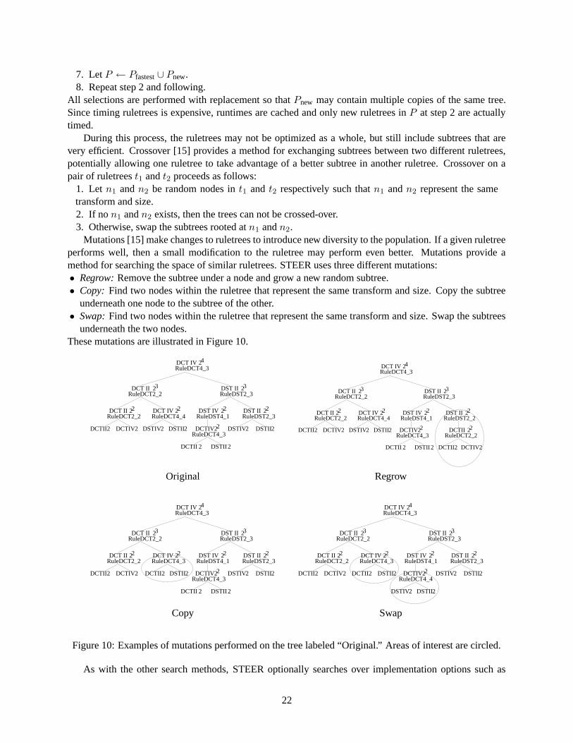
Mutations [15] make changes to ruletrees to introduce new diversity to the population. If a given ruletreeperforms well, then a small modification to the ruletree may perform even better. Mutations provide amethod for searching the space of similar ruletrees. STEER uses three different mutations:• Regrow: Remove the subtree under a node and grow a new random subtree.• Copy: Find two nodes within the ruletree that represent the same transform and size. Copy the subtree

underneath one node to the subtree of the other.• Swap: Find two nodes within the ruletree that represent the same transform and size. Swap the subtrees

underneath the two nodes.These mutations are illustrated in Figure 10.

22� 22� 22� 22�

2323

24

22�

RuleDCT4_3

RuleDST2_3

DST IV

DCT II

RuleDCT2_2DCT II

RuleDCT4_4DCT IV

RuleDCT2_2

RuleDST4_1 RuleDST2_3DST II

DST II

RuleDCT4_3

DCT IV

DCTII DCTIV DSTIV DSTII

DSTIIDCTII

2 2 2 2DCTIV2DSTII2DSTIV

2 2

22� 22� 22� 22�

2323

24

22� 22�

RuleDCT4_3

RuleDST2_3

DST IV

DCT II

RuleDCT2_2DCT II

RuleDCT4_4DCT IV

RuleDCT2_2

RuleDST4_1DST II

DST II

RuleDCT4_3

DCT IV

DCTII DCTIV

DSTII

2 2 DCTIV2DSTII2DSTIV

2 2DCTII

RuleDST2_2

DCTIIRuleDCT2_2

2DCTIV2DCTII

Original Regrow

22� 22� 22� 22�

2323

24

22�RuleDCT4_3

DSTIIDCTII 2 2

RuleDCT4_3

RuleDST2_3

DST IV

DCT II

RuleDCT2_2DCT II DCT IV

RuleDCT2_2

RuleDST4_1 RuleDST2_3DST II

DST II

DCT IV

DCTII DCTIV DSTIV DSTII2 2 2 2DCTIV

RuleDCT4_3

2DSTII2DCTII

22� 22� 22� 22�

2323

24

22�

RuleDCT4_3

RuleDST2_3

DST IV

DCT II

RuleDCT2_2DCT II DCT IV

RuleDCT2_2

RuleDST4_1 RuleDST2_3DST II

DST II

DCT IV

DCTII DCTIV DSTIV DSTII2 2 2 2DCTIV

RuleDCT4_3

2DSTII2DSTIV

RuleDCT4_42DSTII2DCTII

Copy Swap

Figure 10: Examples of mutations performed on the tree labeled “Original.” Areas of interest are circled.

As with the other search methods, STEER optionally searches over implementation options such as

22

the unrolling strategy. For example, enabling a “local unrolling” option determines, for each node in theruletree, whether it should be translated into loop code or unrolled code. The unrolling decisions within aruletree are subject to mutations within reasonable limits.

STEER explores a larger portion of the space of ruletrees than dynamic programming, while still re-maining tractable. Thus, STEER often finds faster formulas than dynamic programming, at the small costof a more expensive search.

5.5 Hill Climbing Search

Hill climbing is a refinement of random search, but is not as sophisticated as STEER. First, hill climbinggenerates a random ruletree and times it. Then, it randomly mutates this ruletree with the mutations definedfor STEER, and times the resulting ruletree. If the new ruletree is faster, hill climbing continues by applyinga mutation to the new ruletree and the process is repeated. Otherwise, if the original ruletree was faster,hill climbing applies another random mutation to the original ruletree and the process is repeated. After acertain number of mutations, the process is restarted with a completely new random ruletree.

5.6 Timed Search

When there is a limited time for search, SPIRAL’s search engine has an integrated approach that combinesthe above search methods to find a fast implementation in the given time. Timed search takes advantageof the strengths of the different search methods, while limiting the search. It is completely configurable,so that a user can specify which search methods are used and how long they are allowed to run. SPIRALprovides reasonable defaults. These defaults first run a random search over a small number of ruletrees tofind a reasonable implementation. Then it calls dynamic programming since this search method often findsgood ruletrees in a relatively short time. Finally, if time remains, it calls STEER to search an even largerportion of the search space.

5.7 Integration and Implementation

All search methods above have been implemented in SPIRAL. As with the formula generator (Section 3),the search engine is implemented entirely in GAP. The search engine uses the ruletree representation ofalgorithms as its only interface to the formula generator. Thus, all search methods are immediately availablewhen new transforms or new rules are added to SPIRAL.

6 Experimental Results

In this section, we present a number of experiments we have conducted using the SPIRAL system version3.1 [22]. Table 2 shows the computing platforms we used for the experiments. In the remainder of thissection we refer to the machines by the name given in the first column.

All timings for the transform implementations generated by SPIRAL are obtained by taking the meanvalue of a sufficiently large number of repeated evaluations. As C compiler options, we used “-O6 -fomit-frame-pointer -malign-double -fstrict-aliasing -mcpu=pentiumpro” for gcc, “-fast -xO5 -dalign” for cc, and“-G6 -O3” and “-G7 -O3” for the Intel compiler on the Pentium III and the Pentium 4, respectively.

The experimental data presented in this section, as well as in Section 2.3, illustrate the following keypoints: 1) The fully-expanded formulas in the algorithm space for DSP transforms have a wide range ofperformance and formulas with the best performance are rare (see Figure 2). 2) The best formula is platformdependent. The best formula on one machine is usually not the best formula on another machine. Searchcan be used to adapt the given platform by finding formulas well suited to that platform. This is shown

23

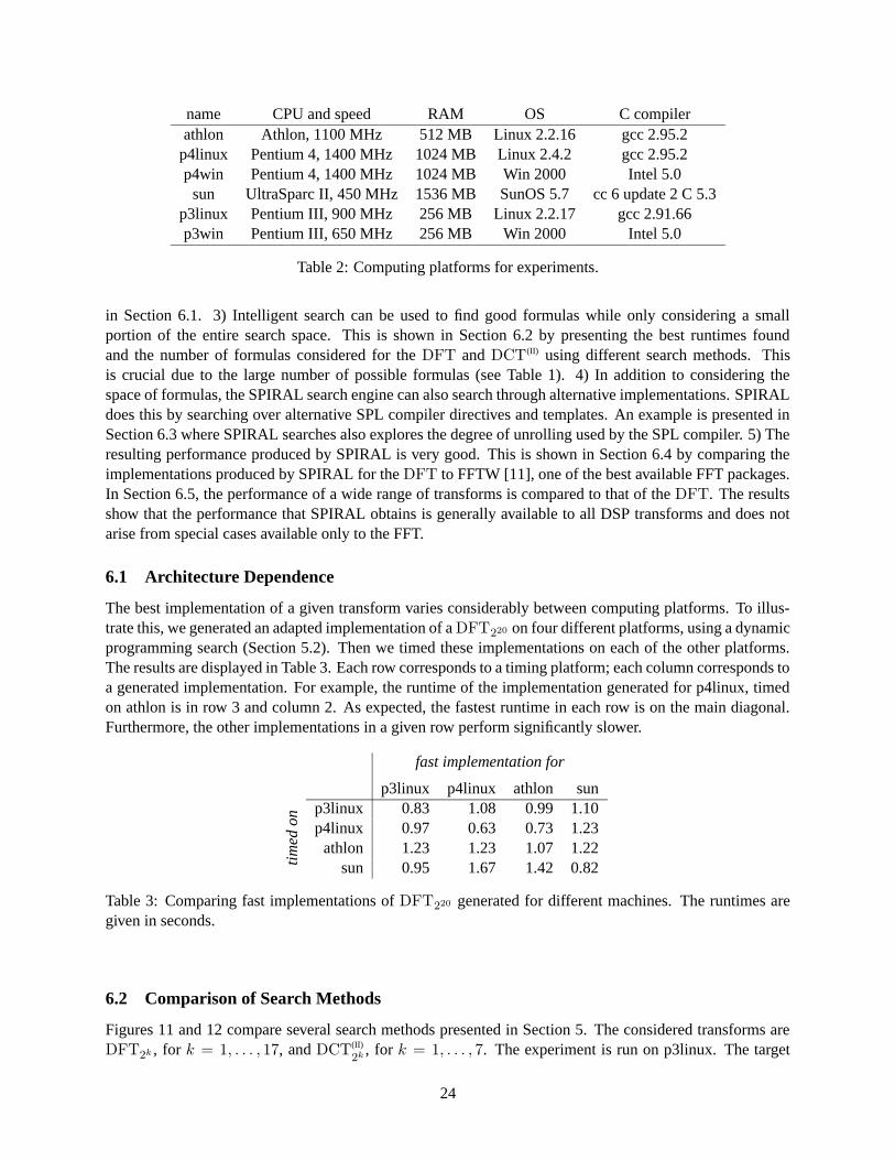
name CPU and speed RAM OS C compilerathlon Athlon, 1100 MHz 512 MB Linux 2.2.16 gcc 2.95.2

p4linux Pentium 4, 1400 MHz 1024 MB Linux 2.4.2 gcc 2.95.2p4win Pentium 4, 1400 MHz 1024 MB Win 2000 Intel 5.0

sun UltraSparc II, 450 MHz 1536 MB SunOS 5.7 cc 6 update 2 C 5.3p3linux Pentium III, 900 MHz 256 MB Linux 2.2.17 gcc 2.91.66p3win Pentium III, 650 MHz 256 MB Win 2000 Intel 5.0

Table 2: Computing platforms for experiments.

in Section 6.1. 3) Intelligent search can be used to find good formulas while only considering a smallportion of the entire search space. This is shown in Section 6.2 by presenting the best runtimes foundand the number of formulas considered for the DFT and DCT(II) using different search methods. Thisis crucial due to the large number of possible formulas (see Table 1). 4) In addition to considering thespace of formulas, the SPIRAL search engine can also search through alternative implementations. SPIRALdoes this by searching over alternative SPL compiler directives and templates. An example is presented inSection 6.3 where SPIRAL searches also explores the degree of unrolling used by the SPL compiler. 5) Theresulting performance produced by SPIRAL is very good. This is shown in Section 6.4 by comparing theimplementations produced by SPIRAL for the DFT to FFTW [11], one of the best available FFT packages.In Section 6.5, the performance of a wide range of transforms is compared to that of the DFT. The resultsshow that the performance that SPIRAL obtains is generally available to all DSP transforms and does notarise from special cases available only to the FFT.

6.1 Architecture Dependence

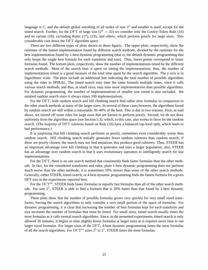
The best implementation of a given transform varies considerably between computing platforms. To illus-trate this, we generated an adapted implementation of a DFT220 on four different platforms, using a dynamicprogramming search (Section 5.2). Then we timed these implementations on each of the other platforms.The results are displayed in Table 3. Each row corresponds to a timing platform; each column corresponds toa generated implementation. For example, the runtime of the implementation generated for p4linux, timedon athlon is in row 3 and column 2. As expected, the fastest runtime in each row is on the main diagonal.Furthermore, the other implementations in a given row perform significantly slower.

fast implementation for

p3linux p4linux athlon sunp3linux 0.83 1.08 0.99 1.10p4linux 0.97 0.63 0.73 1.23

athlon 1.23 1.23 1.07 1.22

tim

edon

sun 0.95 1.67 1.42 0.82

Table 3: Comparing fast implementations of DFT220 generated for different machines. The runtimes aregiven in seconds.

6.2 Comparison of Search Methods

Figures 11 and 12 compare several search methods presented in Section 5. The considered transforms areDFT2k , for k = 1, . . . , 17, and DCT(II)

2k , for k = 1, . . . , 7. The experiment is run on p3linux. The target

24

language is C, and the default global unrolling of all nodes of size 25 and smaller is used, except for thetimed search. Further, for the DFT of large size (2k > 32) we consider only the Cooley-Tukey Rule (16)and its variant (18), excluding Rules (17), (19), and others, which perform poorly for large sizes. Thisconsiderably cuts down the DFT algorithm space.

There are two different types of plots shown in these figures. The upper plots, respectively, show theruntimes of the fastest implementation found by different search methods, divided by the runtimes for thebest implementation found by 1-best dynamic programming (that is, the default dynamic programming thatonly keeps the single best formula for each transform and size). Thus, lower points correspond to fasterformulas found. The bottom plots, respectively, show the number of implementations timed by the differentsearch methods. Most of the search time is spent on timing the implementations; thus, the number ofimplementations timed is a good measure of the total time spent by the search algorithm. The y-axis is inlogarithmic scale. The plots include an additional line indicating the total number of possible algorithmsusing the rules in SPIRAL. The timed search may time the same formula multiple times, since it callsvarious search methods, and thus, at small sizes, may time more implementations than possible algorithms.For dynamic programming, the number of implementations of smaller size timed is also included. Weomitted random search since it always times 100 implementations.

For the DFT, both random search and hill climbing search find rather slow formulas in comparison tothe other search methods at many of the larger sizes. In several of these cases however, the algorithms foundby random search are still within a reasonable 30–40% of the best. This is due to two reasons. First, as saidabove, we turned off some rules for large sizes that are known to perform poorly. Second, we do not drawuniformly from the algorithm space (see Section 5.3), which, in this case, also works in favor for the randomsearch. (The majority of DFT ruletrees based on Rule (16) have a balanced top-level split, which leads tobad performance.)

It is surprising that hill climbing search performs so poorly, sometimes even considerably worse thanrandom search. Hill climbing search initially generates fewer random ruletrees than random search; ifthese are poorly chosen, the search may not find mutations that produce good ruletrees. Thus, STEER hasan important advantage over hill climbing in that it generates and uses a larger population; also, STEERhas an advantage over random search in that it uses evolutionary operators to intelligently search for fastimplementations.

For the DFT, there is no one search method that consistently finds faster formulas than the other meth-ods. In fact, for the considered transforms and rules, plain 1-best dynamic programming does not performmuch worse than the other methods; it is sometimes 10% slower than some of the other search methods.Generally, either STEER, timed search, or 4-best dynamic programming finds the fastest formula for a givenDFT size in the experiments reported here.

For the DCT(II), STEER finds faster formulas or equally fast formulas than all of the other search meth-ods. For size 27, STEER is able to find a formula that is 20% faster than that found by 1-best dynamicprogramming.

These plots show that the number of possible formulas grows very quickly for very small sized trans-forms, forcing the search algorithms to only consider a very small portion of the space of formulas. Fordynamic programming, it is clear that increasing the number of best formulas kept for each transform andsize increases the number of formulas that must be timed. For small sizes, timed search usually times themost formulas as it calls several search algorithms. Since, in the presented experiments, timed search is onlyallowed 30 minutes, it begins to time slightly fewer formulas at larger sizes as it requires more time to runlarger sized formulas. For larger sizes of the DFT, 4-best dynamic programming times the most formulasof all the search algorithms. For DCT(II) sizes 25 to 27, STEER times the most formulas.

25

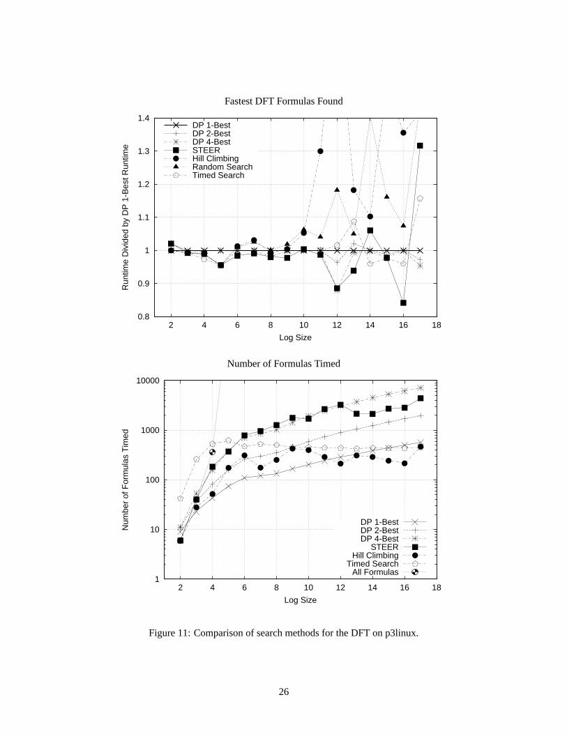
Fastest DFT Formulas Found

0.8

0.9

1

1.1

1.2

1.3

1.4

2 4 6 8 10 12 14 16 18

Run

time

Div

ided

by

DP

1-B

est R

untim

e

Log Size

DP 1-BestDP 2-BestDP 4-BestSTEERHill ClimbingRandom SearchTimed Search

Number of Formulas Timed

1

10

100

1000

10000

2 4 6 8 10 12 14 16 18

Num

ber

of F

orm

ulas

Tim

ed

Log Size

DP 1-BestDP 2-BestDP 4-Best

STEERHill Climbing

Timed SearchAll Formulas

Figure 11: Comparison of search methods for the DFT on p3linux.

26

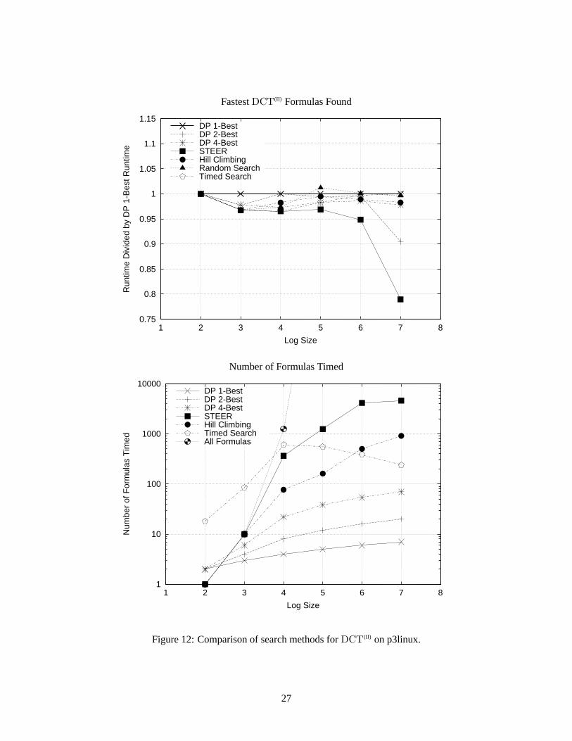
Fastest DCT(II) Formulas Found

0.75

0.8

0.85

0.9

0.95

1

1.05

1.1

1.15

1 2 3 4 5 6 7 8

Run

time

Div

ided

by

DP

1-B

est R

untim

e

Log Size

DP 1-BestDP 2-BestDP 4-BestSTEERHill ClimbingRandom SearchTimed Search

Number of Formulas Timed

1

10

100

1000

10000

1 2 3 4 5 6 7 8

Num

ber

of F

orm

ulas

Tim

ed

Log Size

DP 1-BestDP 2-BestDP 4-BestSTEERHill ClimbingTimed SearchAll Formulas

Figure 12: Comparison of search methods for DCT(II) on p3linux.

27

6.3 Searching over Local Unrolling Settings

Figure 13 compares several of the search methods when also searching over local unrolling settings for theDFT. STEER and 1-best and 4-best dynamic programming were run on the same machine as the experimentsin Section 6.2; this time, the search methods also explored the possible local unrolling settings. Sections 4and 5 describe how this is accomplished. The plots in Figure 13 compare these new runs against the previousruns that used a fixed global unrolling setting.

For many of the smaller sizes of the DFT, the searches that explored the possible local unrolling set-tings found faster implementations than those that used a fix global unrolling setting. The price paid is thenumber of timed formulas, which is much larger compared to searching with fixed global unrolling set-ting. Thus, if search time is not an issue, allowing a search over local unrolling settings can produce fasterimplementations.

6.4 Comparison with FFTW

Figure 14 compares the performance of the best SPIRAL implementation of the DFT to FFTW 2.1.3 on allof the computing platforms considered for sizes 21 to 222. For other transforms highly tuned code is notreadily available. We observe that for various machines and various sizes SPIRAL is faster than FFTW andvice versa. For small DFT sizes, FFTW code is slower due to its more complicated infrastructure. Thesame reason seems to favor SPIRAL code on p4win where the Intel vendor compiler can perform additionaloptimizations on SPIRAL’s simple loop code. The main point in this comparison is not that one is faster thanthe other (without additional analysis and careful consideration of error in timing experiments a definitiveconclusion can not be drawn presently), but rather that the runtimes produced by the general SPIRAL systemare comparable across a range of platforms and transform sizes to FFTW.

6.5 Performance of Different Transforms

Figure 15 shows the performance of the best implementations of different transforms found by SPIRAL onthe Sun machine. The transforms include different types of trigonometric transforms, the Walsh-Hadamardtransform and the (rationalized) Haar transform. The performance of these transforms for sizes 2 to 64 iscompared to the best time for the DFT of the same size. Since the performance of these transforms arecomparable to that of the DFT and it was shown in Section 6.4 that the SPIRAL DFT times are comparableto the best available FFT packages, we can conclude that good performance is obtained across transforms.Figure 15 shows that the other transforms are faster than the DFT beyond size 4, with the WHT and RHTbeing the fastest. This is to be expected since these transforms operate on real data whereas the DFToperates on complex data. That the DFT is faster for sizes 2 and 4 may be due to special optimizations thathave been applied to the DFT.

7 Conclusions

We presented the main components of SPIRAL, a system that automatically generates platform-adaptedimplementations of linear DSP transforms. At the core of SPIRAL is the representation of algorithmsfor transforms as mathematical formulas using a few constructs and primitives. This insight motivates thedesign of the language SPL, which is a domain-specific language for (linear) DSP algorithms. The SPLcompiler translates algorithms, written in SPL, into C or Fortran procedures, and thus connects the math-ematical realm of algorithms with the realm of concrete implementations. The space of algorithms for agiven transform is very large, and yet generated from a small set of rules, which makes possible the au-tomatic generation of these algorithms, and, furthermore, makes it easy to include new transforms. Since

28

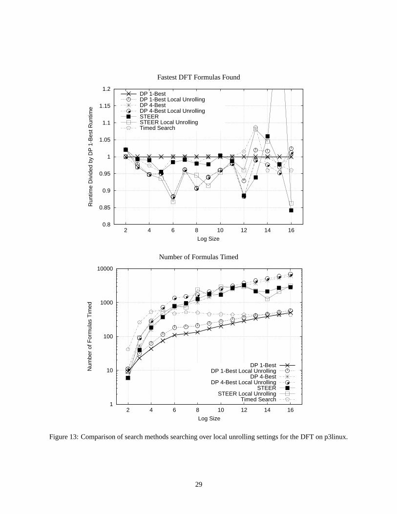
Fastest DFT Formulas Found

0.8

0.85

0.9

0.95

1

1.05

1.1

1.15

1.2

2 4 6 8 10 12 14 16

Run

time

Div

ided

by

DP

1-B

est R

untim

e

Log Size

DP 1-BestDP 1-Best Local UnrollingDP 4-BestDP 4-Best Local UnrollingSTEERSTEER Local UnrollingTimed Search

Number of Formulas Timed

1

10

100

1000

10000

2 4 6 8 10 12 14 16

Num

ber

of F

orm

ulas

Tim

ed

Log Size

DP 1-BestDP 1-Best Local Unrolling

DP 4-BestDP 4-Best Local Unrolling

STEERSTEER Local Unrolling

Timed Search

Figure 13: Comparison of search methods searching over local unrolling settings for the DFT on p3linux.

29

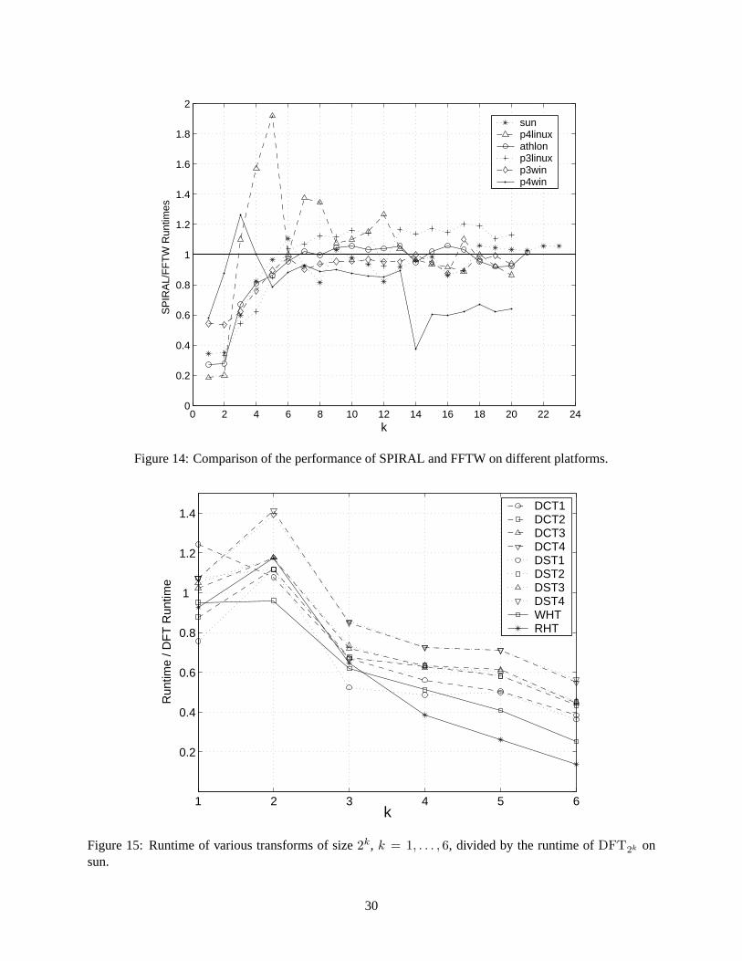
0 2 4 6 8 10 12 14 16 18 20 22 240

0.2

0.4

0.6

0.8

1

1.2

1.4

1.6

1.8

2

k

SP

IRA

L/F

FT

W R

untim

es

sunp4linuxathlonp3linuxp3winp4win

Figure 14: Comparison of the performance of SPIRAL and FFTW on different platforms.

1 2 3 4 5 6

0.2

0.4

0.6

0.8

1

1.2

1.4

k

Run

time

/ DF

T R

untim

e

DCT1DCT2DCT3DCT4DST1DST2DST3DST4WHTRHT

Figure 15: Runtime of various transforms of size 2k, k = 1, . . . , 6, divided by the runtime of DFT2k onsun.

30

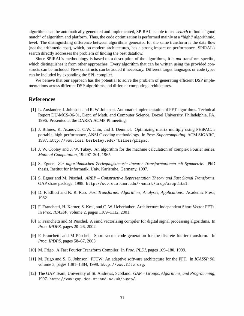
algorithms can be automatically generated and implemented, SPIRAL is able to use search to find a “goodmatch” of algorithm and platform. Thus, the code optimization is performed mainly at a “high,” algorithmic,level. The distinguishing difference between algorithms generated for the same transform is the data flow(not the arithmetic cost), which, on modern architectures, has a strong impact on performance. SPIRAL’ssearch directly addresses the problem of finding the best dataflow.

Since SPIRAL’s methodology is based on a description of the algorithms, it is not transform specific,which distinguishes it from other approaches. Every algorithm that can be written using the provided con-structs can be included. New constructs can be added if necessary. Different target languages or code typescan be included by expanding the SPL compiler.

We believe that our approach has the potential to solve the problem of generating efficient DSP imple-mentations across different DSP algorithms and different computing architectures.

References

[1] L. Auslander, J. Johnson, and R. W. Johnson. Automatic implementation of FFT algorithms. TechnicalReport DU-MCS-96-01, Dept. of Math. and Computer Science, Drexel University, Philadelphia, PA,1996. Presented at the DARPA ACMP PI meeting.

[2] J. Bilmes, K. Asanovic, C.W. Chin, and J. Demmel. Optimizing matrix multiply using PHiPAC: aportable, high-performance, ANSI C coding methodology. In Proc. Supercomputing. ACM SIGARC,1997. http://www.icsi.berkeley.edu/~bilmes/phipac.

[3] J. W. Cooley and J. W. Tukey. An algorithm for the machine calculation of complex Fourier series.Math. of Computation, 19:297–301, 1965.

[4] S. Egner. Zur algorithmischen Zerlegungstheorie linearer Transformationen mit Symmetrie. PhDthesis, Institut fur Informatik, Univ. Karlsruhe, Germany, 1997.

[5] S. Egner and M. Puschel. AREP – Constructive Representation Theory and Fast Signal Transforms.GAP share package, 1998. http://www.ece.cmu.edu/∼smart/arep/arep.html.

[6] D. F. Elliott and K. R. Rao. Fast Transforms: Algorithms, Analyses, Applications. Academic Press,1982.

[7] F. Franchetti, H. Karner, S. Kral, and C. W. Ueberhuber. Architecture Independent Short Vector FFTs.In Proc. ICASSP, volume 2, pages 1109–1112, 2001.

[8] F. Franchetti and M Puschel. A simd vectorizing compiler for digital signal processing algorithms. InProc. IPDPS, pages 20–26, 2002.

[9] F. Franchetti and M Puschel. Short vector code generation for the discrete fourier transform. InProc. IPDPS, pages 58–67, 2003.

[10] M. Frigo. A Fast Fourier Transform Compiler. In Proc. PLDI, pages 169–180, 1999.

[11] M. Frigo and S. G. Johnson. FFTW: An adaptive software architecture for the FFT. In ICASSP 98,volume 3, pages 1381–1384, 1998. http://www.fftw.org.

[12] The GAP Team, University of St. Andrews, Scotland. GAP – Groups, Algorithms, and Programming,1997. http://www-gap.dcs.st-and.ac.uk/∼gap/.

31

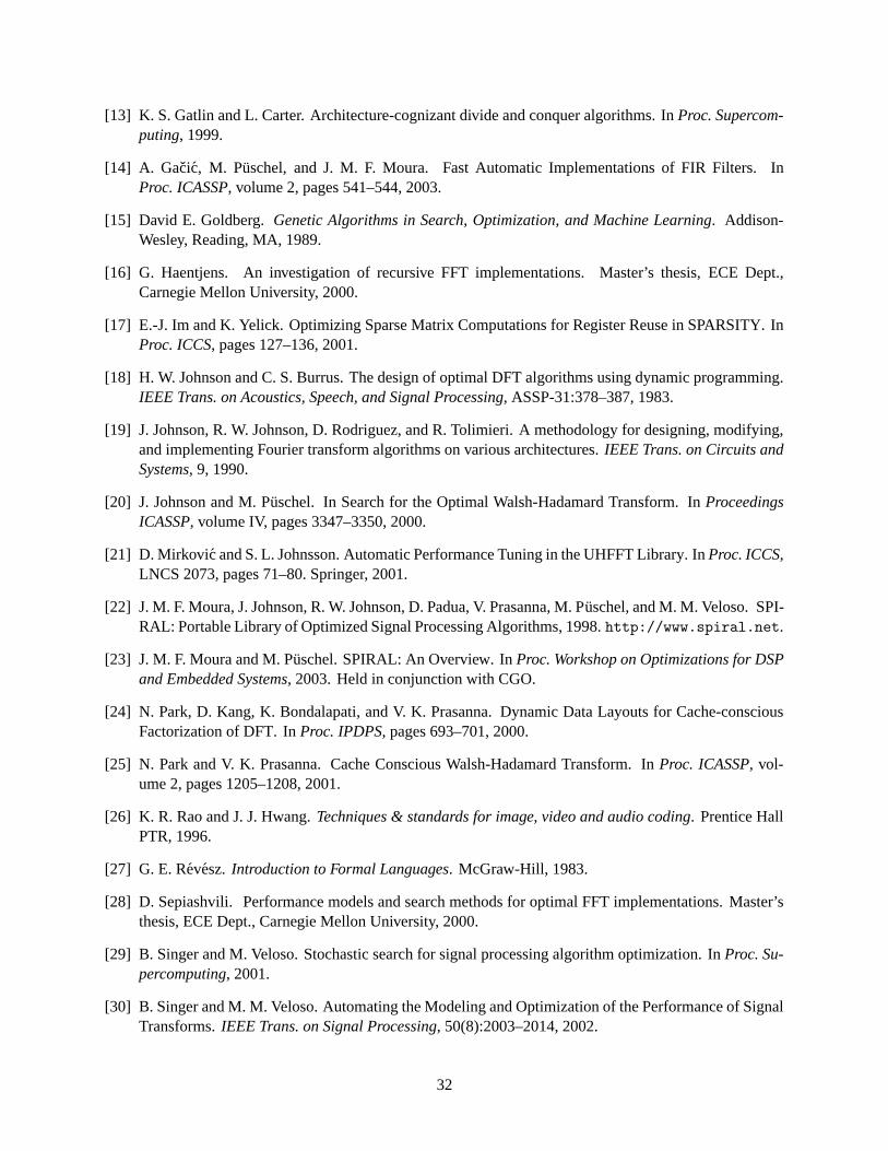
[13] K. S. Gatlin and L. Carter. Architecture-cognizant divide and conquer algorithms. In Proc. Supercom-puting, 1999.

[14] A. Gacic, M. Puschel, and J. M. F. Moura. Fast Automatic Implementations of FIR Filters. InProc. ICASSP, volume 2, pages 541–544, 2003.

[15] David E. Goldberg. Genetic Algorithms in Search, Optimization, and Machine Learning. Addison-Wesley, Reading, MA, 1989.

[16] G. Haentjens. An investigation of recursive FFT implementations. Master’s thesis, ECE Dept.,Carnegie Mellon University, 2000.

[17] E.-J. Im and K. Yelick. Optimizing Sparse Matrix Computations for Register Reuse in SPARSITY. InProc. ICCS, pages 127–136, 2001.

[18] H. W. Johnson and C. S. Burrus. The design of optimal DFT algorithms using dynamic programming.IEEE Trans. on Acoustics, Speech, and Signal Processing, ASSP-31:378–387, 1983.

[19] J. Johnson, R. W. Johnson, D. Rodriguez, and R. Tolimieri. A methodology for designing, modifying,and implementing Fourier transform algorithms on various architectures. IEEE Trans. on Circuits andSystems, 9, 1990.

[20] J. Johnson and M. Puschel. In Search for the Optimal Walsh-Hadamard Transform. In ProceedingsICASSP, volume IV, pages 3347–3350, 2000.

[21] D. Mirkovic and S. L. Johnsson. Automatic Performance Tuning in the UHFFT Library. In Proc. ICCS,LNCS 2073, pages 71–80. Springer, 2001.

[22] J. M. F. Moura, J. Johnson, R. W. Johnson, D. Padua, V. Prasanna, M. Puschel, and M. M. Veloso. SPI-RAL: Portable Library of Optimized Signal Processing Algorithms, 1998. http://www.spiral.net.

[23] J. M. F. Moura and M. Puschel. SPIRAL: An Overview. In Proc. Workshop on Optimizations for DSPand Embedded Systems, 2003. Held in conjunction with CGO.

[24] N. Park, D. Kang, K. Bondalapati, and V. K. Prasanna. Dynamic Data Layouts for Cache-consciousFactorization of DFT. In Proc. IPDPS, pages 693–701, 2000.

[25] N. Park and V. K. Prasanna. Cache Conscious Walsh-Hadamard Transform. In Proc. ICASSP, vol-ume 2, pages 1205–1208, 2001.

[26] K. R. Rao and J. J. Hwang. Techniques & standards for image, video and audio coding. Prentice HallPTR, 1996.

[27] G. E. Revesz. Introduction to Formal Languages. McGraw-Hill, 1983.

[28] D. Sepiashvili. Performance models and search methods for optimal FFT implementations. Master’sthesis, ECE Dept., Carnegie Mellon University, 2000.

[29] B. Singer and M. Veloso. Stochastic search for signal processing algorithm optimization. In Proc. Su-percomputing, 2001.

[30] B. Singer and M. M. Veloso. Automating the Modeling and Optimization of the Performance of SignalTransforms. IEEE Trans. on Signal Processing, 50(8):2003–2014, 2002.

32

[31] R. Tolimieri, M. An, and C. Lu. Algorithms for discrete Fourier transforms and convolution. Springer,2nd edition, 1997.

[32] C. Van Loan. Computational Framework of the Fast Fourier Transform. Siam, 1992.

[33] M. Vetterli and H.J. Nussbaumer. Simple FFT and DCT Algorithms with reduced Number of Opera-tions. Signal Processing, 6:267–278, 1984.

[34] Z. Wang. Fast Algorithms for the Discrete W Transform and for the Discrete Fourier Transform. IEEETrans. on Acoustics, Speech, and Signal Processing, ASSP-32(4):803–816, 1984.

[35] Z. Wang and B.R. Hunt. The Discrete W Transform . Applied Mathematics and Computation, 16:19–48, 1985.

[36] R. C. Whaley and J. Dongarra. Automatically Tuned Linear Algebra Software (ATLAS). In Proc. Su-percomputing, 1998. http://math-atlas.sourceforge.net/.

[37] J. Xiong. Automatic Optimization of DSP Algorithms. PhD thesis, Computer Science, Universityof Illinois at Urbana-Champaign, 2001. Also as Tech. Report UIUCDCS-R-2001-224, University ofIllinois.

[38] J. Xiong, J. Johnson, R. Johnson, and D. Padua. SPL: A Language and Compiler for DSP Algorithms.In Proc. PLDI, pages 298–308, 2001.

33