Speed scaling: An algorithmic perspective

Adam Wierman∗ Lachlan L. H. Andrew† Minghong Lin‡

Abstract

Speed scaling has long been used as a power-saving mechanism at a chip level. However, in recent years, speedscaling has begun to be used as an approach for trading off energy usage and performance throughout all levels ofcomputer systems. This wide-spread use of speed scaling has motivated significant research on the topic, but manyfundamental questions about speed scaling are only beginning to be understood. In this chapter, we focus on a simple,but general, model of speed scaling and provide an algorithmic perspective on four fundamental questions: (i) Whatis the structure of the optimal speed scaling algorithm? (ii) How does speed scaling interact with scheduling? (iii)What is the impact of the sophistication of speed scaling algorithms? and (iv) Does speed scaling have any unintendedconsequences? For each question we provide a summary of insights from recent work on the topic in both worst-caseand stochastic analysis as well as a discussion of interesting open questions that remain.

1 IntroductionComputer systems must make a fundamental tradeoff between performance and energy usage. The days of “faster isbetter” are gone — energy usage can no longer be ignored in designs, from chips to mobile devices to data centers.This has led speed scaling, a technique once only applied in microprocessors, to become an important technique at alllevels of systems. At this point, speed scaling is quickly being adopted across systems from chips [1] to disks [2] anddata centers [3] to wireless devices [4].

Speed scaling works by adapting the “speed” of the system to balance energy and performance. It can be highlysophisticated — adapting the speed at all times to the current state (dynamic speed scaling) — or very simple —running at a static speed chosen a priori to balance energy and performance, except when idle (gated-static speedscaling) as used in current disk drives [5].

Dynamic speed scaling leads to many challenging algorithmic problems. Fundamentally, when implementingspeed scaling, an algorithm must make two decisions at each time: (i) a scheduling policy decides which job(s) toserve, and (ii) a speed scaler decides how fast to run. Further, there is an unavoidable interaction between thesedecisions.

The growing adoption of speed scalers and the inherent complexity of their design has led to a significant, and stillgrowing analytic literature studying the design and performance of speed scaling algorithms. The analytic study ofthe speed scaling problem began with the seminal work of [6] in 1995. Since [6], three main performance objectiveshave emerged: (i) the total energy used in order to meet job deadlines, e.g., [7, 8] (ii) the average response time givenan energy/power budget, e.g., [9, 10], and (iii) a linear combination of expected response time and energy usage perjob [11, 12].

The goal of this chapter is not to provide a complete survey of analytic work on speed scaling. For such purposeswe recommend the reader consult the recent survey [13] in addition to the current chapter. Instead, the goal of thecurrent chapter is to provide examples of the practical insights about fundamental issues in speed scaling that comefrom the analytic work. Consequently, to limit the scope of the chapter, we focus on only the third performanceobjective listed above, a linear combination of response time and energy usage, which captures how much reductionin response time justifies using one extra joule and applies where there is a known monetary cost to extra delay (e.g.,many web applications). Note that (iii) is related to (ii) by duality. Further, we additionally simplify the settingconsidered in this chapter by studying only a simple, single resource model, which is described in detail in Section 2.∗Computer and Mathematical Sciences, California Institute of Technology, adamw@caltech.edu†Centre for Advanced Internet Architectures, Swinburne University of Technology, landrew@swin.edu.au‡Computer and Mathematical Sciences, California Institute of Technology, mhlin@caltech.edu

1

Through the simplifications described above, we avoid complexity in the model and can focus on the insightsprovided by the results we survey. More specifically, we focus on four fundamental issues in speed scaling design forwhich recent analytic results have been able to provide new, practical insights.

I What structure do (near-)optimal algorithms have? Can an online speed scaling algorithm be optimal?

II How does speed scaling interact with scheduling?

III How important is the sophistication of the speed scaler? What benefits come from using dynamic versus staticspeed scaling?

IV What are the drawbacks of speed scaling?

To provide insight into these issues, we provide an overview of recent work from two analytic frameworks – worst-case analysis and stochastic analysis. For each question we provide a summary of insights from both worst-case andstochastic analysis as well as a discussion of interesting open questions that remain. To conclude the introductionwe provide a brief, informal overview of the insights into Issues I-IV that follow from recent results in the analyticcommunity. The remainder of the chapter will then provide a more formal description of the results and insightsreferred to briefly below.

Issue I: The analytic results we survey prove that “energy-proportional” speed scaling provides near-optimalperformance. Specifically, by using sn, the speed to run at given n jobs, such that P (sn) = nβ (where P (s) is thepower needed to run at speed s and 1/β is the price of energy) it is possible to be 2-competitive for general P ; that is,to incur a total cost at most twice the optimum obtainable by a system will full prior knowledge. This provides analyticjustification for a common heuristic applied by system designers, e.g., [14]. However, note that this algorithm does notmatch the offline optimal performance. In fact, no “natural” speed scaling algorithm (see Definition 1) can be betterthan 2-competitive; hence no online energy-proportional speed scaler matches the offline optimal. Thus, optimizingfor energy and delay is, in some sense, fundamentally harder than optimizing for delay alone.1

Issue II: The analytic results we survey related to Issue II uncover two useful insights. First, at least among thepolicies analyzed so far, speed scaling can be decoupled from scheduling in that energy-proportional speed scalingprovides nearly optimal performance for three common scheduling policies. Second, scheduling is not as importantonce energy is considered. Specifically, scheduling policies that are not constant competitive for delay alone becomeO(1)-competitive for the linear combination of energy and response time once speed scaling is considered. Theseinsights allow designers to deal individually with two seemingly coupled design decisions.

Issue III: The analytic results we survey highlight that increased sophistication provides minimal performanceimprovements in speed scaling designs. More specifically, the optimal gated-static speed scaling performs nearly aswell as the optimal dynamic speed scaler. However, increased sophistication does provide improved robustness. Theseinsights have the practical implication that it may be better to design “optimally robust” speeds instead of “optimal”speeds, since robustness is the main benefit of dynamic scaling.

Issue IV: The analytic results we survey show that, unfortunately, dynamic speed scaling can magnify unfairness.This is perhaps surprising at first, but follows intuitive from the fact that dynamic speed scaling selects faster speedswhen there are more jobs in the system: If some property of a job is correlated with the occupancy while it is in service,then dynamic speed scaling gives an unfairly high service rate to jobs with that property. In contrast to the conclusionfor Issue II, these results highlight that designers should be wary about the interaction between the scheduler and speedscaler when considering fairness.

2 Model and notationTo highlight the insights that follow from analytic results, we focus on a simple, single server model and ignore manypractical issues such as deadlines and the costs of switching speeds. It is important to emphasize however that thereis a broad literature of analytic work that has begun to study the impact of such issues, and we do our best to givepointers to this work.

Throughout this chapter we consider a single server with two control decisions: speed scaling and scheduling.Further, we take as the performance objective the minimization of a linear combination of expected response time

1A simple, greedy policy (Shortest Remaining Processing Time) optimizes mean delay in a single server system of fixed rate [15].

2

(also called sojourn time or flow time), denoted by T , and energy usage per job, E :

z = E[T ] + E[E ]/β. (1)

Using Little’s law, this may be more conveniently expressed as

λz = E[N ] + E[P ]/β (2)

where N is the number of jobs in the system and P = λE is the power expended.Note that though we take a linear combination of energy and response time as our performance metric, there

are a wide variety of other metrics that have been studied in the speed scaling literature. The first to be studied inan algorithmic context was minimizing the total energy consumption given deadlines for each job [6, 16, 17]. In thissetting, the energy reduction incurs no performance penalty, since it is assumed that there is no benefit to finishing jobsbefore the deadline. Another objective is to minimize the makespan (time to finish all jobs) given a constraint on thetotal energy [17,18]. This is called the “laptop problem”, since the constrained energy consumption matches the fixedcapacity of a portable device’s battery. Circuit designers are often interested in the product of power and delay [19],which represents the energy per operation. Many other formulations have been considered, such as minimizing delaygiven a trickle-charged energy storage [20], and cases in which jobs need not be completed but can provide revenuedependent on their delay [21].

Further, though we focus only on a single server, there is recent work that studies speed scaling in multiserverenvironments as well: in the context of jobs with deadlines [22, 23], the laptop problem [17], or with the aboveobjective [23–26].

2.1 Modeling energy usageTo model the energy usage, first let n(t) denote the number of jobs in the system at time t and s(t) denote the speedthat the system is running at time t. Further, define P (s) as the power needed to run at speed s. Then, the energy usedby time t is E(t) =

∫ t0P (s(τ))dτ .

In many applications P (s) ≈ ksα with α ∈ (1, 3). For example, for dynamic power in CMOS chips α ≈ 1.8 [27].However, wireless communication has an exponential P [28] or even unbounded power at finite rate [29]. Some ofthe results we discuss assume a polynomial form, and simplify specifically for α = 2. Others hold for general, evennon-convex and discontinuous, power functions. Several results are limited to regular power functions [12], which aredifferentiable on [0,∞), strictly convex, non-negative, and P (0) = 0.

Note that implicit in the model above is that all jobs have the same P (s). In practice, different classes of jobs mayhave different mixes of requirements for CPU, disk, IO, etc. This leads to each class of jobs having a different P (s)function characterizing its power-speed tradeoff curve.

2.2 Modeling speed scaling and schedulingA speed scaling algorithm A = (π,Σ) consists of a scheduling discipline π that defines the order in which jobs areprocessed, and a speed scaler Σ that defines the speed as a function of system state, in terms of the power function, P .Throughout, we consider the speed to depend only on the number of jobs in the system, i.e., sn is the speed when theoccupancy is n.2

We consider online preempt-resume schedulers, which are not aware of a job j until it arrives at time r(j), at whichpoint they learn its size, xj , and which may interrupt serving a job and later restart it from the point it was interruptedwithout overhead. We focus on Shortest Remaining Processing Time (SRPT), which preemptively serves the jobwith the least remaining work, and Processor Sharing (PS), which serves all jobs in the system at equal rate. SRPTis important due to its optimality properties: in a classical, constant speed system, SRPT minimizes the expectedresponse time [15]. PS is important because it is a simple model of scheduling that is commonly applied for, e.g.,operating systems and web servers. A third policy that we discuss occasionally is First Come First Served (FCFS),which serves jobs in order of arrival.

The speed scaling rules, sn, we consider can be gated-static, which runs at a constant speed while the systemis non-empty and sleeps while the system is empty, i.e., sn = sgs1n 6=0; or more generally dynamic sn = g(n) for

2This suits objective (1); e.g., it is optimal for an isolated batch arrival, and the optimal s is constant between arrival/departures. For otherobjectives, it is better to base the speed on the unfinished work instead [30].

3

some function g : N ∪ 0 → [0,∞). To be explicit, we occasionally write sπn as the speed under policy π when theoccupancy is n. The queue is single-server in the sense that the full speed sn can be devoted to a single job.

2.3 Analytic frameworkAnalytic research studying speed scaling has used two distinct approaches: worst-case analysis and stochastic analysis.We discuss results from both settings in this paper, and so we briefly introduce the settings and notation for each in thefollowing.

Notation for the worst-case model

In the worst-case model we consider finite, arbitrary (maybe adversarial) deterministic instances of ν arriving jobs.Let E(I) be the total energy used to complete instance I , and Tj be the response time of job j, the completion timeminus the release time r(j). The analog of (1) is to replace the ensemble average by the sample average, giving thecost of an instance I under a given algorithm A as

zA(I) =1

ν

(∑jTj +

1

βE(I)

). (3)

In this model, we compare the cost of speed scaling algorithms to the cost of the optimal offline algorithm, OPT. Inparticular, we study the competitive ratio, defined as

CR = supIzA(I)/zO(I),

where zO(I) is the optimal cost achievable on I . A scheme is “c-competitive” if its competitive ratio is at most c.

Notation for the stochastic model

In the stochastic model, we consider an M/GI/1 (or sometimes GI/GI/1) queue with arrival rate λ. Let X denote arandom job size with cumulative distribution function (c.d.f.) F (x), complementary c.d.f. (c.c.d.f.) F (x) = 1−F (x),and continuous probability density function (p.d.f.) f(x) = dF (x)/dx. Let ρ = λE[X] ∈ [0,∞) denote the loadof arriving jobs. Note that ρ is not the utilization of the system and that many dynamic speed scaling algorithms arestable for all ρ. When the power function is P (s) = sα, it is natural to use a scaled load, γ := ρ/β1/α (see [27]).

Denote the response time of a job of size x by T (x). We consider the performance metric (1) where the expectationsare averages per job. In this model the goal is to optimize this cost for a specific workload, ρ. Let zO be the averagecost of the optimal offline algorithm. and define the competitive ratio in the M/GI/1 model as

CR = supF,λ

zA/zO.

3 Optimal speed scalingThe most natural starting point for discussing speed scaling algorithms is to understand:

What structure do (near-)optimal algorithms have? Can a speed scaling algorithm be optimal?

In this section, we discuss the stream of research that has sought to answer these questions.To begin, recall that a speed scaling algorithm depends on two choices, the scheduler and the speed scaler. How-

ever, when determining the optimal speed scaling algorithm, the optimality properties of SRPT in the static speedsetting [15] make it a natural choice for the scheduler. In fact, it is easy to argue that any speed scaling algorithm whichdoes not use SRPT can be improved by switching the scheduler to SRPT and leaving the speeds s(t) unchanged [12].

Thus, in this section we focus on speed scaling algorithms that use SRPT scheduling and seek to understand thestructure of the (near-)optimal speeds. The study of optimal speed scaling algorithms has primarily been performed inthe worst-case analytic framework. The reason for this is simple: SRPT is difficult to analyze in the stochastic modeleven in the case when the speed is fixed. So, when dynamic, controllable speeds are considered the analysis is, to thispoint, seemingly intractable.

4

However, in the worst-case framework considerable progress has been made. The focus of this research has pri-marily been on one particularly promising algorithm: (SRPT, P−1(n)), which uses policy π = SRPT and speed scalerΣ which sets sn = P−1(n), and there has been a stream of upper bounds on its competitive ratio for objective (1): forunit-size jobs in [11, 30] and for general jobs with P (s) = sα in [31, 32]. A major breakthrough was made in [12],which shows the 3-competitiveness of (SRPT, P−1(n+1)) for general P . Following this breakthrough, [33] was ableto use similar techniques to reduce the competitive ratio slightly and prove a matching lower bound. In particular, [33]establishes the following:

Theorem 1. For any regular power function P , (SRPT, P−1(nβ)) has a competitive ratio of exactly 2.

Thus, (SRPT, P−1(n)) is not optimal, in that an offline algorithm could do better. However, it is highly robust —guaranteeing to provide cost within a factor of two of optimal.

We will not dwell on the analytic approaches in this chapter, however it is useful to give some feel for the prooftechniques for the major results. In this case, the proof uses amortized local competitiveness arguments with thepotential function

Φ(t) =

∫ ∞0

n[q;t]∑i=1

1 + η

βP ′(P−1 (iβ)

)dq, (4)

where n[q; t] = max(0, nA[q; t] − nO[q; t]) with nA[q; t] and nO[q; t] the number of unfinished jobs at time t withremaining size at least q under (SRPT,P−1(nβ)) (algorithm A) and the optimal (offline) algorithm O, respectively.Specifically, it first shows that

zA(t) +dΦ

dt≤ (1 + η)zO(t), (5)

where zA(t) and zO(t) are the instantaneous costs ofA and O respectively, given by n(t) +P (s(t))/β. It then showsthat integrating this, with η = 1, gives the above theorem.

The following more general form can be proven analogously.

Corollary 2. Let η ≥ 1 and Φ be given by (4). Any scheme A = (SRPT, sn) with sn ∈ [P−1(nβ), P−1(ηnβ)] is(1 + η)-competitive.

The above results motivate the question:

Are there other speed scaling algorithms with lower competitive ratios?

A recent result [33] suggests that the answer is “No”. In particular, no “natural” speed scaling algorithm can bebetter than 2-competitive.

Definition 1. A speed scaling algorithmA is defined to be natural if it runs at speed sn when it has n unfinished jobs,and for convex P , one of the following holds:

(a) the scheduler is work-conserving and works on a single job between arrival/departure events; or

(b) g(s) + P (s)/β is convex, for some g with g(sn) = n; or

(c) the speeds sn satisfy P (sn) = ω(n); or

(d) the speeds sn satisfy P (sn) = o(n).

Theorem 3. For any ε > 0 there is a regular power function Pε such that any natural algorithm A on Pε hascompetitive ratio larger than 2− ε.

Note that natural algorithms include SRPT scheduling for any sn, energy-proportional speeds for all schedulersand any speeds consistently faster or slower than energy-proportional. We conjecture that Theorem 3 holds for allspeed scaling algorithms, which would imply that the competitive ratio of (SRPT, P−1(nβ)) is minimal.

Interestingly, the proof considers only two classes of workloads: one consisting of an isolated burst of jobs andthe other consisting of a long train of uniformly spaced jobs. Any “natural” scheduler which processes the long trainfast enough to avoid excessive delay costs must process the burst so fast that it incurs excessive energy costs; thusoptimizing over these two specific workloads is already impossible for a “natural” speed scaler.

5

3.1 Open questionsThe results above highlight that that energy-proportional speed scaling (P (sn) = nβ) is nearly optimal, which pro-vides analytic justification of a common design heuristic, e.g., [14]. Further, they highlight that optimizing for thecombination of energy and delay is fundamentally harder than optimizing for delay alone (where SRPT is optimal,i.e., 1-competitive). However, they also leave a number of interesting and important questions unanswered. Threesuch questions that are particularly interesting are the following.

First, the fact that Theorem 3 holds only for “natural” algorithms is bothersome and likely only a technical restric-tion. It would be very nice to remove this restriction and provide a true lower bound on the achievable competitiveratio.

Additionally, the fact that (SRPT,P−1(n)) is exactly 2-competitive for every power function highlights that it maybe possible to outperform this algorithm for specific power functions. In particular, for the realistic case of P (s) = sα

with α ∈ (1, 3) it is possible to derive other speed scalers besides P−1(n) that have competitive ratios smaller than2. In the extreme case that P is concave, it is optimal to run at the maximum possible speed whenever there is workin the system, and be idle otherwise. It would be interesting to understand in general what the lower bound on theachievable competitive ratio for a fixed P (s) is, and what speed scaler can achieve it.

Finally, a third open problem is to understand the optimal speeds for SRPT scheduling in the stochastic model,i.e., in an M/GI/1 queue. This problem is completely open, and seemingly difficult, but would provide interesting newinsight.

These three open questions all relate to the simple model which is the focus of this chapter; however the issuesdiscussed in this section are clearly also interesting (and open) when the model is made more complex. For example,by allowing class-dependent P (s) functions.

4 The interaction of speed scaling and schedulingIn the prior section, we focused on optimal speed scaling algorithms, and thus limited our attention to SRPT. However,in practice, SRPT may not be appropriate, for a variety of reasons. In many situations, other scheduling policies aredesirable (or required) and in particular, policies such as PS are used. Once a different scheduling policy is consideredit is not clear how the optimal speeds should be adjusted. In particular, there is a clear coupling between the speedscaling and the scheduling. So, the focus of this section is to understand:

How does speed scaling interact with scheduling?

To shed light on this question we focus primarily on PS in this section, due to its importance in application suchas operating systems and web servers. However, the insights we describe certainly hold more generally.

There is work relating to the interaction of scheduling and speed scaling from both the worst-case and stochasticframeworks, so we will discuss each briefly. Interestingly, the two distinct sets of results highlight similar insights. Inparticular they highlight that (i) scheduling and speed scaling can be largely decoupled with minimal performance lossand (ii) scheduling is much less important when considering speed scaling than it is in standard models with constantspeeds.

4.1 Worst-case analysisIn contrast to the long stream of research focusing on SRPT, until recently there was no worst-case analysis of speedscaling under PS. The first result relating to PS is from [33], which shows that (PS, P−1(nβ)) is O(1)-competitive forP (s) = sα with fixed α. In particular:

Theorem 4. If P (s) = sα then (PS, P−1(nβ)) is max(4α− 2, 2(2− 1/α)α)-competitive.

As with SRPT, this admits a more general corollary

Corollary 5. For sn given in Corollary 2, the scheme (PS, sn) is O(1)-competitive in the size of the instance.

Notice that the competitive ratio in Theorem 4 reduces to (4α − 2)-competitive for the α typical in CPUs, i.e.,α ∈ (1, 3].

6

The proof of Theorem 4 in [33] builds on the analysis in [34] of LAPS, another blind policy. (LAPS, P−1(nβ))is also O(1)-competitive in this case, and actually has better asymptotic performance for large α. However, as α ∈(1, 3] in most computer sub-systems, the performance for small α is more important than asymptotics in α, and PSoutperforms LAPS in that case. In both the case of PS and LAPS the proof uses the potential function

Φ = (1 + η)(2α− 1)(H/β)1/αnA(t)∑i=1

i1−1/α max(0, qA(ji; t)− qO(ji; t)) (6)

where qπ(j; t) is the remaining work on job j at time t under scheme π ∈ A, O, and jinA(t)i=1 is an ordering of the

jobs in increasing order of release time: r(j1) ≤ r(j2) ≤ · · · ≤ r(jnA(t)).This result has been generalized in [35] to show that weighted PS is again O(1)-competitive in the case when jobs

have differing weights. If the processor has a maximum speed, then the result still holds under a resource augmentationassumption.

There are a number of remarks we would like to highlight about Theorem 4. First, notice that this scheme usesthe same energy-proportional speeds sn = P−1(nβ) that achieve the optimal competitive ratio under SRPT. Further,the same speeds are also used for LAPS in [34]. This suggests that the two design decisions of speed scaling andscheduling are not as closely coupled as may be first thought.

A second remark about Theorem 4 is that, although this competitive ratio of around 10 is larger than may be hoped,it is very much smaller than the competitive ratio of PS on a fixed-speed processor. On a fixed-speed processor, PShas an unbounded competitive ratio: PS is Ω(ν1/3)-competitive for instances with ν jobs [36]. This is because PS is“blind” to the job sizes, which can cause it to make a poor decision early on, from which it can never recover. Withunbounded speeds and dynamic speed scaling, the processor can always run a little faster to recover quickly, and thuscontinue with a modest additional cost. Note however, that difference in cost across scheduling policies grows if thereis a bounded maximum speed.

To explain the limited impact of scheduling, one can view speed scaling as a physical realization of the analyticaltechnique of resource augmentation [37]. The latter shows that many algorithms with high competitive ratios couldachieve almost the same cost as the optimal algorithm, if they were given the advantage of a slightly faster processor.

Finally, a third remark about Theorem 4 is that it is much weaker than Theorem 1 for SRPT: Not only is the com-petitive ratio larger, but the result is only valid for power functions of the form P (s) = sα, and even depends stronglyon the exponent α. This is not simply because the result is incomplete, but because the problem is fundamentally lesswell approximable. In fact, all policies blind to job sizes have unbounded competitive ratio as α → ∞ [34], whichshows that the form of power function must unavoidably enter any competitive ratio result.

4.2 Stochastic analysisIn contrast to the limited amount of research studying PS in the worst-case framework, there has been a substantialamount of work applicable to PS in the stochastic framework, due to its analytic tractability. In particular, in theM/GI/1 model, [38–41]3 study speed scaling in the context of generic “operating costs”.

This work formulates the determination of the optimal speeds as a dynamic programming (DP) problem andprovides numerical techniques for determining the optimal speeds. Further, it has been proven that the optimal speedsare monotonic in the queue length [43] and that the optimal speeds can be bounded as follows [27]. Recall thatγ = ρ/β1/α.

Proposition 6. Consider an M/GI/1 PS queue with controllable service rates sn. Let P (s) = sα. The optimal dynamicspeeds are concave and satisfy the dynamic program given in [27]. For α = 2 and any n ≥ 2γ, they satisfy

γ +√n− 2γ ≤ sDPn√

β≤ γ +

√n+ min

( γ2n, γ1/3

). (7)

3Since M/GI/1 PS with controllable service rates is symmetric [42], it has the same occupancy distribution and mean delay as M/M/1 FCFSstudied in the references.

7

For general α > 1, they satisfy

sDPnβ1/α

≤(

n

α− 1

)1/α

+ γ1

α− 1+O(n−1/α) (8)

sDPnβ1/α

≥(

n

α− 1

)1/α

. (9)

Interestingly, the bounds in Proposition 6 are tight for large n and have a form similar to the form of the worst-casespeeds for SRPT and PS in Theorems 1 and 4.

The asymptotic form of these results also matches the form of the optimal speed when there are n jobs in thesystem and no more jobs will arrive before the queue is emptied, as occurs when the instance is a single batch arrival.For both SRPT and PS, this batch speed is given by the solution s∗n to

βn = s∗nP′(s∗n)− P (s∗n). (10)

This is not surprising, since when the backlog is large, the arrival rate will be negligible compared with the optimalspeed. This insight is further supported by looking at the fluid model, e.g., [44], where the differences betweenscheduling policies are negligible.

As we have discussed previously, the analysis of the optimal dynamic speeds given SRPT scheduling is seeminglyintractable. However, taking inspiration from the fact that the speeds given by the worst-case analysis of SRPT andPS match, combined with the fact that (10) is the optimal batch speed for both SRPT and PS and also matches theasymptotic form of the stochastic results for PS in Proposition 6, a natural proposal for the dynamic speeds underSRPT is to use the optimal PS speeds.

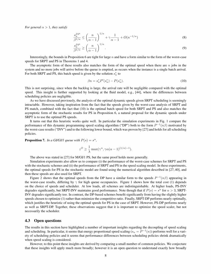
It turns out that this heuristic works quite well. In particular the simulation experiments in Fig. 1 compare theperformance of this dynamic programming speed scaling algorithm (“DP”) both to the form P−1(nβ) motivated bythe worst-case results (“INV”) and to the following lower bound, which was proven by [27] and holds for all schedulingpolicies.

Proposition 7. In a GI/GI/1 queue with P (s) = sα,

zO ≥ 1

λmax(γα, γα(α− 1)(1/α)−1).

The above was stated in [27] for M/GI/1 PS, but the same proof holds more generally.Simulation experiments also allow us to compare (i) the performance of the worst-case schemes for SRPT and PS

with the stochastic schemes and (ii) the performance of SRPT and PS in the speed scaling model. In these experiments,the optimal speeds for PS in the stochastic model are found using the numerical algorithm described in [27, 40], andthen these speeds are also used for SRPT.

Figure 2 shows that the optimal speeds from the DP have a similar form to the speeds P−1(nβ) appearing inthe worst-case results, differing by γ for high queue occupancies. Figure 1 shows how the total cost (1) dependson the choice of speeds and scheduler. At low loads, all schemes are indistinguishable. At higher loads, PS-INVdegrades significantly, but SRPT-INV maintains good performance. Note though that if P (s) = sα for α > 3, SRPT-INV degrades significantly too. In contrast, the DP-based schemes benefit significantly from having the slightly higherspeeds chosen to optimize (1) rather than minimize the competitive ratio. Finally, SRPT-DP performs nearly optimally,which justifies the heuristic of using the optimal speeds for PS in the case of SRPT. However, PS-DP performs nearlyas well as SRPT-DP. Together, these observations suggest that it is important to optimize the speed scaler, but notnecessarily the scheduler.

4.3 Open questionsThe results in this section have highlighted a number of important insights regarding the decoupling of speed scalingand scheduling. In particular, it seems that energy proportional speed scaling (sn = P−1(n)) performs well for a vari-ety of scheduling policies and it seems that performance differences between scheduling policies shrink dramaticallywhen speed scaling is considered.

However, to this point these insights are derived by comparing a small number of common policies. We conjecturethat these insights will apply much more broadly; however it is an open question to understand exactly how broadly

8

1/16 1/4 0 4 16 640

10

20

30

40

50

60

γ

cost

PS−INV

PS−DP

SRPT−INV

SRPT−DP

LowerBound

(a)

1/16 1/4 0 4 16 640

1

2

3

4

γ

cost/lo

werb

ound

PS−INV

PS−DP

SRPT−INV

SRPT−DP

(b)

Figure 1: Comparison of SRPT and PS under both sn = P−1(nβ) and speeds optimized for an M/GI/1 PS system,using Pareto(2.2) job sizes and P (s) = s2.

they apply. More specifically, it would be interesting to characterize the class of scheduling policies for which sn =P−1(n) guarantees O(1)-competitiveness. This would jointly highlight a decoupling between scheduling and speedscaling and show that scheduling has much less impact on performance. The above question proposes to study thedecoupling of scheduling and speed scaling in the worst-case framework. In the stochastic framework however, theparallel question can be asked: for what class of policies will sn = P−1(n) guarantee O(1)-competitiveness in theM/GI/1 model.

5 Impact of speed scaler sophisticationUp until this point we have focused on dynamic speed scaling, which allows the speed to change as a function ofthe number of jobs in the system. Dynamic speed scaling can perform nearly optimally; however its complexity maybe prohibitive. In contrast, gated-static speed scaling, where sn = sgs1n 6=0 for some constant speed sgs, requiresminimal hardware to support; e.g., a CMOS chip may have a constant clock speed but AND it with the gating signalto set the speed to 0.

In this section our goal is to understand:

How important is the sophistication of the speed scaler? What benefits come from using dynamic versusstatic speed scaling?

Note that we can immediately see that gated-static speed scaling can be arbitrarily bad in the worst case since jobscan arrive faster than sgs. Thus, we study gated-static speed scaling only in the stochastic model, where the constantspeed sgs can depend on the load.

We focus our discussion on SRPT and PS, though the insights we highlight do not depend on the workings of theseparticular policies and should hold more generally.

Overall, there are three main insights that have emerged from the literature regarding the questions above. First, andperhaps surprisingly, the simplest policy (gated-static) provides nearly the same expected cost as the most sophisticatedpolicy (optimal dynamic scaling). Second, the performance of gated-static under PS and SRPT are not too different,thus scheduling is less important to optimize than in systems in which the speed is fixed in advance. This alignswith the observations discussed in the previous section for the case of dynamic speed scaling. Third, though dynamicspeed scaling does not provide significantly improved cost, it does provide significantly improved robustness (e.g., totime-varying and/or uncertain workloads).

9

5.1 Optimal gated-static speedsTo begin our discussion, we must first discuss the optimal speeds to use for gated-static designs under both PS andSRPT. In the case of PS, this turns out to be straightforward; however in the case of SRPT it is not.

Before stating the results, note that since the power cost is constant at P (sgs) whenever the server is running, theoptimal speed is

sgs = arg minsβE[T ] +

1

λP (s) Pr(N 6= 0). (11)

In the second term Pr(N 6= 0) = ρ/s, and so multiplying by λ and setting the derivative to 0 gives that the optimalgated-static speed satisfies

βdE[N ]

ds+ r

P ∗(s)

s= 0, (12)

where r = ρ/s is the utilization and P ∗(s) ≡ sP ′(s)−P (s). Note that if P is convex then P ∗ is increasing and if P ′′

is bounded away from 0 then P ∗ is unbounded.Under PS, E[N ] = ρ/(s− ρ), and so dE[N ]/ds = E[N ]/(ρ− s). By (12), the optimal speeds satisfy [27]

βE[N ] = (1− r)rP ∗(s). (13)

For SRPT, things are not as easy. For s = 1, we have [45]

E[T ] =

∫ ∞x=0

∫ x

t=0

dt

1− λ∫ t

0τ dF (τ)

+λ∫ x

0τ2 dF (τ) + x2F (x)

2(1− λ∫ x

0τdF (τ))2

dF (x)

The complexity of this equation rules out calculating the speeds analytically. So, instead [33] derives simplerforms for E[N ] that are exact in asymptotically heavy or light traffic. Note that using a heavy-traffic approximation isnatural for this setting because, if energy is important (β small), than the speed will be provisioned so that the serveris in “high” load.

We state the heavy-traffic results for distributions whose c.c.d.f. F has lower and upper Matuszewska indices [46]of m and M . Intuitively this means that C1x

m . F (x) . C2xM as x → ∞ for some C1, C2, so the Matuszewska

index can be thought of as a “moment index.” Further, let G(x) =∫ x0tf(t) dt/E[X] be the fraction of work coming

from jobs of size at most x, and define h(r) = (G−1)′(r)/G−1(r). The following was proven in [47].

Proposition 8 ( [47]). For an M/GI/1 under SRPT with speed 1, E[N ] = Θ(H(ρ)) as ρ→ 1, where

H(ρ) =

E[X2]/((1− ρ)G−1(ρ)) if M < −2E[X] log(1/(1− ρ)) if m > −2.

(14)

For the case of unit speed, this suggests the heavy traffic approximation

E[N ] ≈ CH(ρ) (15)

where the constant C depends on the distribution of job sizes.

Theorem 9. Under the assumption that (15) holds with equality:

(i) If M < −2, then for the optimal gated-static speed,

βE[N ]

(2− r1− r

− rh(r)

)= rP ∗(s). (16a)

(ii) If m > −2, then for the optimal gated-static speed,

βE[N ]

(1

(1− r) log(1/(1− r))

)= P ∗(s). (16b)

Moreover, if P ∗(s) is unbounded as s→∞ and −2 6∈ [m,M ] then as ρ→∞, (16) induces the heavy-traffic regime,ρ/s→ 1.

Although the heavy traffic results hold for large ρ, for small ρ the performance of the optimal GS speed for PSgives better performance. To combine these, [33] proposes using the speed

sSRPTgs = min(sPSgs , sSRPT (HT )gs ), (17)

where sPSgs satisfies (13), and sSRPT (HT )gs is given by (16) with E[N ] estimated by (15).

10

0 20 40 60 80 1000

2

4

6

8

10

12

n

sn

DP

INV

Figure 2: Comparison of sn = P−1(nβ) with speeds“DP” optimized for an M/GI/1 system with γ = 1 andP (s) = s2.

0.5 0.9 0.99 0.9990

10

20

30

40

ρ

E[T

]

approximate E[T]

numerical E[T]

Figure 3: Validation of the heavy-traffic approxima-tion (15) by simulation using Pareto(3) job sizes withE[X] = 1.

5.2 Dynamic vs. gated static: cost comparisonGiven the optimal gated static speeds derived in the previous section, we can now contrast the cost of gated-static, thesimplest scheme, with that of dynamic speed scaling, the most sophisticated under both SRPT and PS.

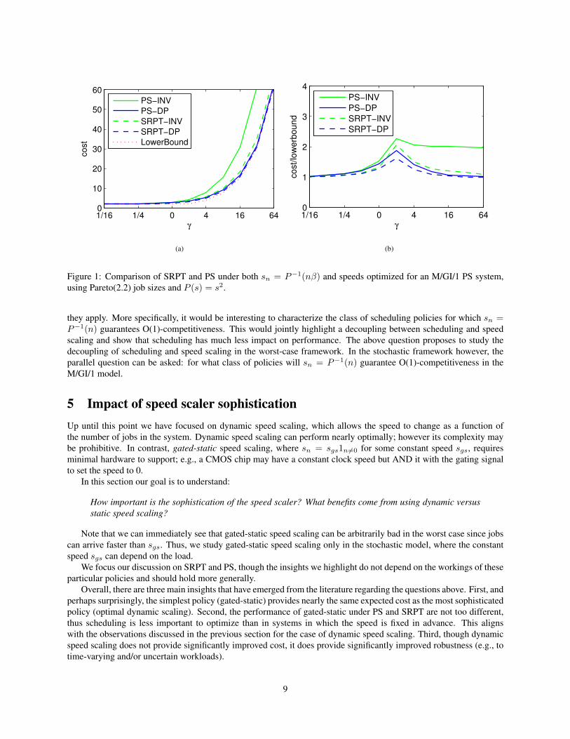
As Fig. 4 shows, the performance of a well-tuned gated-static system is almost indistinguishable from that of theoptimal dynamic speeds. Moreover, there is little difference between the cost under PS-GATED and SRPT-GATED,again highlighting that scheduling becomes less important when speed can be scaled than in traditional models.

Additionally, [27] has recently provided analytic support for the empirical observation that gated-static schemesare near optimal. Specifically, in [27] it was proven that PS-GATED is within a factor of 2 of PS-DP when P (s) = s2.With the results of Section 3, this implies:

Corollary 10. If P (s) = s2 then the optimal PS and SRPT gated-static designs are O(1)-competitive in an M/GI/1queue with load ρ.

5.3 Dynamic vs. gated static: robustness comparisonThe previous section shows that near-optimal performance is obtained by running at a static speed when not idle. Whythen do CPUs have multiple speeds? The reason is that the optimal gated-static design depends intimately on the loadρ. This cannot be exactly known in advance, especially since workloads vary with time. So, an important property ofa speed scaling design is robustness to uncertainty in the workload (ρ and F ) and to model inaccuracies.

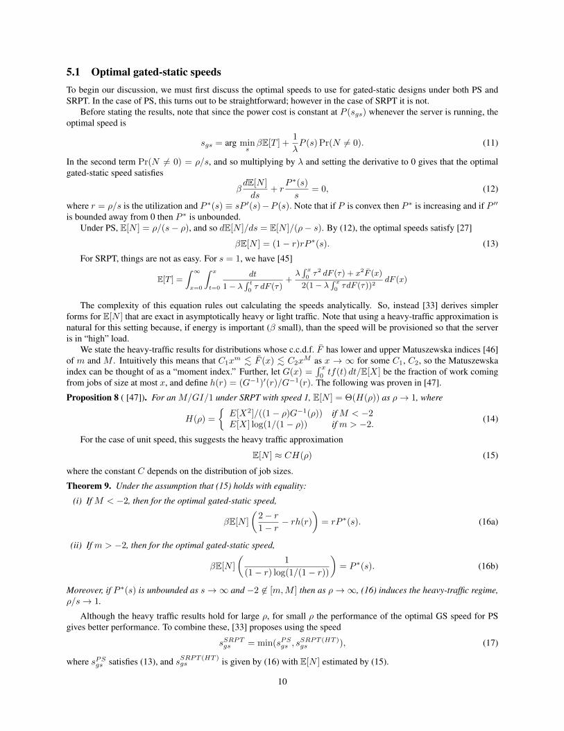
Figure 5 shows that the performance of gated-static degrades dramatically when ρ is mispredicted. If the load islower than expected, excess energy will be used; if the system has static speed s and ρ ≥ s then the cost is unbounded.In contrast, Fig. 5 also shows that dynamic speed scaling (SRPT-DP) is significantly more robust to misprediction ofthe workload.

Recently, [33] proved the robustness of SRPT-DP and PS-DP by providing worst-case guarantees for SRPT-DPand PS-DP showing that they are both constant competitive. These results are nearly unique in that they provideworst-case guarantees for stochastic control policies. In the following, let sDPn denote the speeds used for SRPT-DPand PS-DP.

Corollary 11. Consider P (s) = sα with α ∈ (1, 2] and algorithm A which chooses speeds sDPn optimal for PS in anM/GI/1 queue with load ρ. If A uses either PS or SRPT, then A is O(1)-competitive in the worst-case.

The proof of the result follows from combining (8) and (9) with Corollaries 2 and 5.Notice that for α = 2, Proposition 6 implies sDPn ≤ (2γ + 1)P−1(nβ), whence (SRPT, sDPn ) is (4γ2 + 4γ + 2)-

competitive.Finally, though Corollary 11 shows that sDPn designed for a given ρ leads to a “robust” speed scaler, note that the

cost still degrades significantly when ρ is mispredicted badly (see Fig. 5). To address this issue, we consider a second,

11

1/16 1/4 0 4 16 640

10

20

30

40

50

60

γ

cost

PS−GATED

PS−DP

SRPT−GATED

SRPT−DP

LowerBound

(a)

1/16 1/4 0 4 16 640

1

2

3

4

γ

cost/lo

werb

ound

PS−GATED

PS−DP

SRPT−GATED

SRPT−DP

(b)

Figure 4: Comparison of PS and SRPT with gated-static speeds (13) and (17), versus the dynamic speeds optimal foran M/GI/1 PS. Job sizes are distributed as Pareto(2.2) and P (s) = s2.

0 10 20 30 40

5

10

15

20

design γ

cost

SRPT−GATED

SRPT−DP

SRPT−LIN

(a) SRPT

0 10 20 30 40

5

10

15

20

design γ

cost

PS−GATED

PS−DP

PS−LIN

(b) PS

Figure 5: Effect of misestimating γ under PS and SRPT: cost when γ = 10, but sn are optimal for a different “designγ”. Pareto(2.2) job sizes; P (s) = s2.

12

weaker form of robustness: robustness only to misestimation of ρ, not to the underlying stochastic model. In particular,in this model the arrivals are known to be Poisson, but ρ is unknown. In this setting, it was shown in [27] that using“linear” speeds, sn = n

√β, gives near-optimal performance when P (s) = s2 and PS scheduling is used. Specifically,

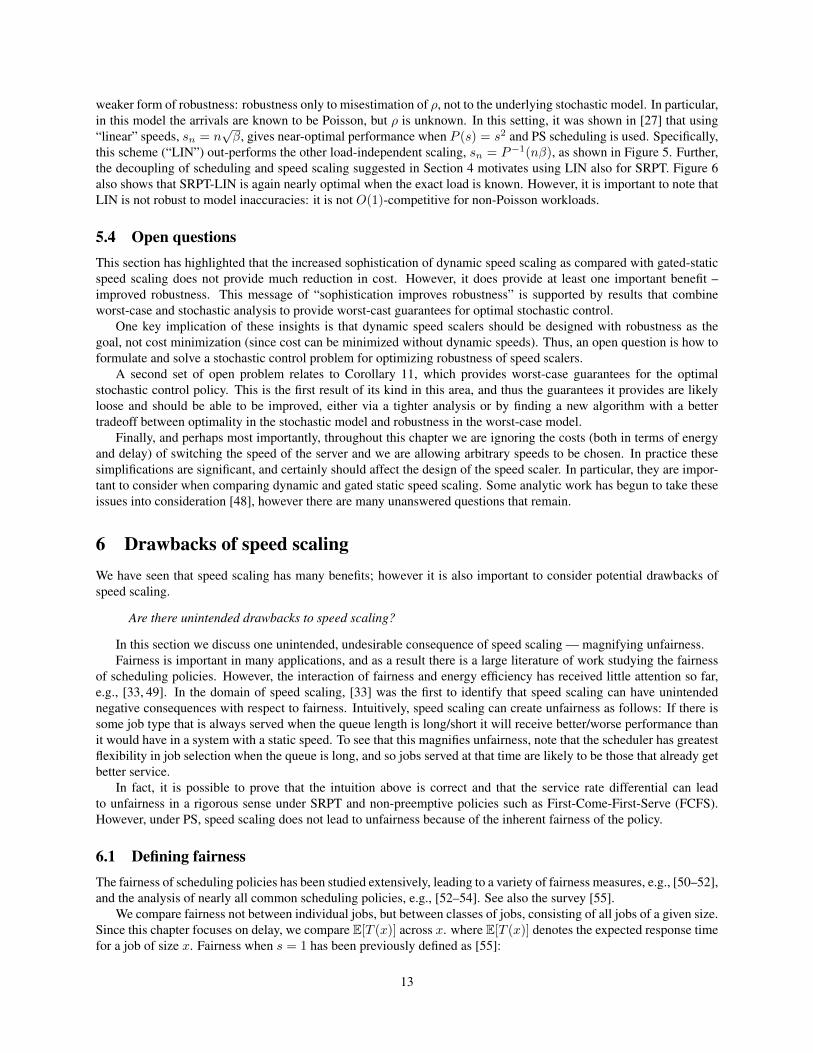
this scheme (“LIN”) out-performs the other load-independent scaling, sn = P−1(nβ), as shown in Figure 5. Further,the decoupling of scheduling and speed scaling suggested in Section 4 motivates using LIN also for SRPT. Figure 6also shows that SRPT-LIN is again nearly optimal when the exact load is known. However, it is important to note thatLIN is not robust to model inaccuracies: it is not O(1)-competitive for non-Poisson workloads.

5.4 Open questionsThis section has highlighted that the increased sophistication of dynamic speed scaling as compared with gated-staticspeed scaling does not provide much reduction in cost. However, it does provide at least one important benefit –improved robustness. This message of “sophistication improves robustness” is supported by results that combineworst-case and stochastic analysis to provide worst-cast guarantees for optimal stochastic control.

One key implication of these insights is that dynamic speed scalers should be designed with robustness as thegoal, not cost minimization (since cost can be minimized without dynamic speeds). Thus, an open question is how toformulate and solve a stochastic control problem for optimizing robustness of speed scalers.

A second set of open problem relates to Corollary 11, which provides worst-case guarantees for the optimalstochastic control policy. This is the first result of its kind in this area, and thus the guarantees it provides are likelyloose and should be able to be improved, either via a tighter analysis or by finding a new algorithm with a bettertradeoff between optimality in the stochastic model and robustness in the worst-case model.

Finally, and perhaps most importantly, throughout this chapter we are ignoring the costs (both in terms of energyand delay) of switching the speed of the server and we are allowing arbitrary speeds to be chosen. In practice thesesimplifications are significant, and certainly should affect the design of the speed scaler. In particular, they are impor-tant to consider when comparing dynamic and gated static speed scaling. Some analytic work has begun to take theseissues into consideration [48], however there are many unanswered questions that remain.

6 Drawbacks of speed scalingWe have seen that speed scaling has many benefits; however it is also important to consider potential drawbacks ofspeed scaling.

Are there unintended drawbacks to speed scaling?

In this section we discuss one unintended, undesirable consequence of speed scaling — magnifying unfairness.Fairness is important in many applications, and as a result there is a large literature of work studying the fairness

of scheduling policies. However, the interaction of fairness and energy efficiency has received little attention so far,e.g., [33, 49]. In the domain of speed scaling, [33] was the first to identify that speed scaling can have unintendednegative consequences with respect to fairness. Intuitively, speed scaling can create unfairness as follows: If there issome job type that is always served when the queue length is long/short it will receive better/worse performance thanit would have in a system with a static speed. To see that this magnifies unfairness, note that the scheduler has greatestflexibility in job selection when the queue is long, and so jobs served at that time are likely to be those that already getbetter service.

In fact, it is possible to prove that the intuition above is correct and that the service rate differential can leadto unfairness in a rigorous sense under SRPT and non-preemptive policies such as First-Come-First-Serve (FCFS).However, under PS, speed scaling does not lead to unfairness because of the inherent fairness of the policy.

6.1 Defining fairnessThe fairness of scheduling policies has been studied extensively, leading to a variety of fairness measures, e.g., [50–52],and the analysis of nearly all common scheduling policies, e.g., [52–54]. See also the survey [55].

We compare fairness not between individual jobs, but between classes of jobs, consisting of all jobs of a given size.Since this chapter focuses on delay, we compare E[T (x)] across x. where E[T (x)] denotes the expected response timefor a job of size x. Fairness when s = 1 has been previously defined as [55]:

13

1/16 1/4 0 4 16 640

10

20

30

40

50

60

γ

cost

PS−LIN

PS−DP

SRPT−LIN

SRPT−DP

LowerBound

(a)

1/16 1/4 0 4 16 640

1

2

3

4

γ

cost/lo

werb

ound

PS−LIN

PS−DP

SRPT−LIN

SRPT−DP

(b) c

Figure 6: Comparison of PS and SRPT with linear speeds, sn = n√β, and with dynamic speeds optimal for PS. Job

sizes are Pareto(2.2) and P (s) = s2.

Definition 2. A policy π is fair if for all x

E[Tπ(x)]

x≤ E[TPS(x)]

x.

This metric is motivated by the fact that (i) PS is intuitively fair since it shares the server evenly among all jobs atall times; (ii) for s = 1, the slowdown (“stretch”) of PS is constant, i.e., E[T (x)]/x = 1/(1−ρ); (iii) E[T (x)] = Θ(x)[56], so normalizing by x when comparing the performance of different job sizes is appropriate. Additional support isprovided by the fact that minπ maxx E[Tπ(x)]/x = 1/(1− ρ) [52].

By this definition, the class of large jobs is treated fairly under all work-conserving policies, i.e., limx→∞ E[T (x)]/x ≤1/(1−ρ) [56] — even policies such as SRPT that seem biased against large jobs. In contrast, all non-preemptive poli-cies, e.g., FCFS have been shown to be unfair to small jobs [52].

The foregoing applies only when s = 1. However, the following Proposition shows that PS still maintains aconstant slowdown for arbitrary speeds, and so Definition 2 is still a natural notion of fairness.

Proposition 12. Consider an M/GI/1 queue with a symmetric scheduling discipline, e.g., PS with controllable servicerates. Then, E[T (x)] = x (E[T ]/E[X]) .

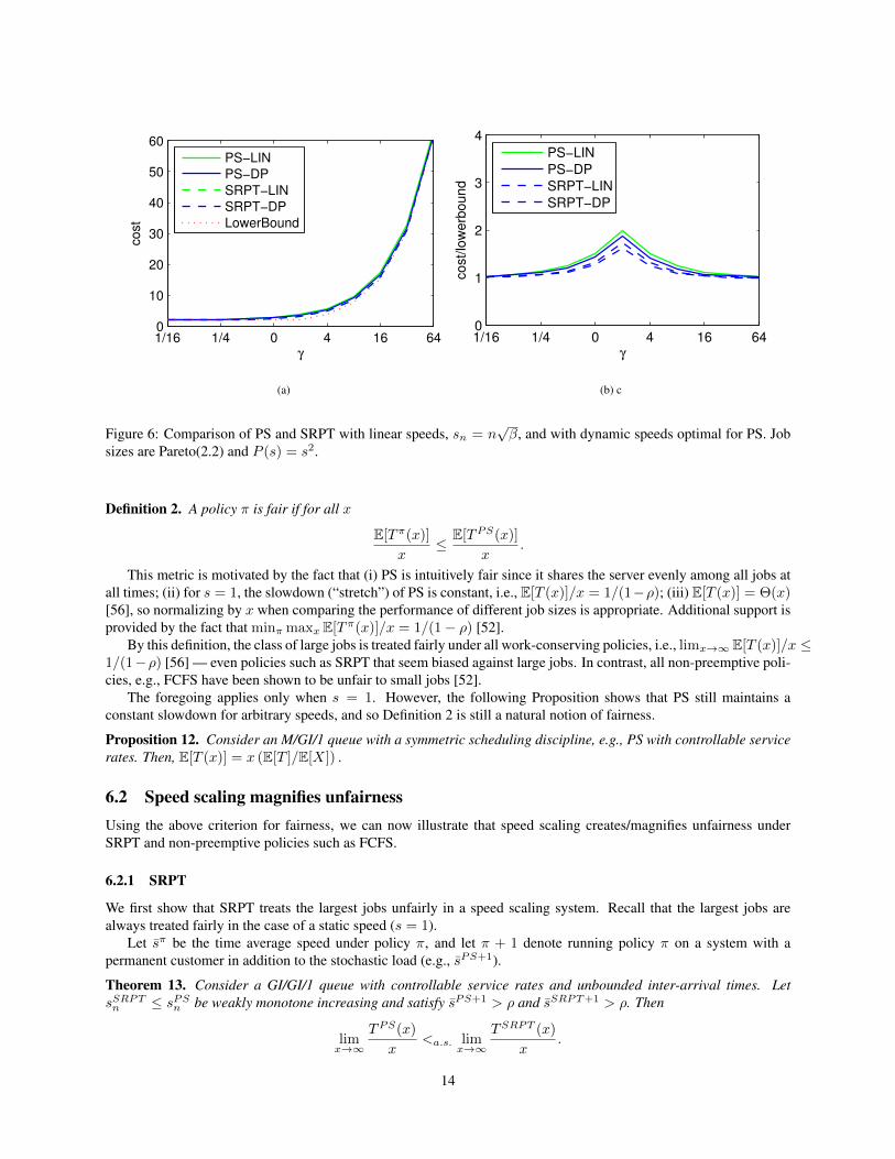
6.2 Speed scaling magnifies unfairnessUsing the above criterion for fairness, we can now illustrate that speed scaling creates/magnifies unfairness underSRPT and non-preemptive policies such as FCFS.

6.2.1 SRPT

We first show that SRPT treats the largest jobs unfairly in a speed scaling system. Recall that the largest jobs arealways treated fairly in the case of a static speed (s = 1).

Let sπ be the time average speed under policy π, and let π + 1 denote running policy π on a system with apermanent customer in addition to the stochastic load (e.g., sPS+1).

Theorem 13. Consider a GI/GI/1 queue with controllable service rates and unbounded inter-arrival times. LetsSRPTn ≤ sPSn be weakly monotone increasing and satisfy sPS+1 > ρ and sSRPT+1 > ρ. Then

limx→∞

TPS(x)

x<a.s. lim

x→∞

TSRPT (x)

x.

14

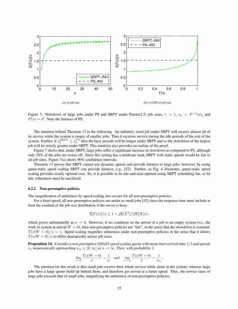
0 10 20 30 40 500

0.5

1

1.5

2

2.5

3

x

E[T

(x)]

/x

SRPT−INV

PS−INV

(a) vs job size

0 0.2 0.4 0.6 0.8 10

0.5

1

1.5

2

2.5

3

F(x)

E[T

(x)]

/x

SRPT−INV

PS−INV

(b) vs CDF of job size

Figure 7: Slowdown of large jobs under PS and SRPT under Pareto(2.2) job sizes, γ = 1, sn = P−1(n), andP (s) = s2. Note the fairness of PS.

The intuition behind Theorem 13 is the following. An infinitely sized job under SRPT will receive almost all ofits service while the system is empty of smaller jobs. Thus it receives service during the idle periods of the rest of thesystem. Further, if sSRPTn ≤ sPSn then the busy periods will be longer under SRPT and so the slowdown of the largestjob will be strictly greater under SRPT. This intuition also provides an outline of the proof.

Figure 7 shows that, under SRPT, large jobs suffer a significant increase in slowdown as compared to PS, althoughonly 10% of the jobs are worse off. Since this setting has a moderate load, SRPT with static speeds would be fair toall job sizes. Figure 7(a) shows 90% confidence intervals.

Theorem 13 proves that SRPT cannot use dynamic speeds and provide fairness to large jobs; however, by usinggated-static speed scaling SRPT can provide fairness, e.g., [52]. Further, as Fig. 4 illustrates, gated-static speedscaling provides nearly optimal cost. So, it is possible to be fair and near-optimal using SRPT scheduling but, to befair, robustness must be sacrificed.

6.2.2 Non-preemptive policies

The magnification of unfairness by speed scaling also occurs for all non-preemptive policies.For a fixed speed, all non-preemptive policies are unfair to small jobs [52] since the response time must include at

least the residual of the job size distribution if the server is busy:

E[T (x)]/x ≥ 1 + ρE[X2]/(2E[X]x),

which grows unboundedly as x → 0. However, if we condition on the arrival of a job to an empty system (i.e., thework in system at arrival W = 0), then non-preemptive policies are “fair”, in the sense that the slowdown is constant:T (x|W = 0)/x = 1. Speed scaling magnifies unfairness under non-preemptive policies in the sense that it allowsT (x|W = 0)/x to differ dramatically across job sizes.

Proposition 14. Consider a non-preemptive GI/GI/1 speed scaling queue with mean inter-arrival time 1/λ and speedssn monotonically approaching s∞ ∈ (0,∞] as n→∞. Then, with probability 1,

limx→0

T (x|W = 0)

x=

1

s1and lim

x→∞

T (x|W = 0)

x=

1

s∞.

The intuition for this result is that small jobs receive their whole service while alone in the system; whereas largejobs have a large queue build up behind them, and therefore get served at a faster speed. Thus, the service rates oflarge jobs exceeds that of small jobs, magnifying the unfairness of non-preemptive policies.

15

6.3 Open questionsThis section has highlighted that dynamic speed scaling has an important drawback – it magnifies unfairness. However,the results summarized here represent only a first step toward understanding this phenomenon. In particular, they onlyhighlight the existence of the phenomenon and say little else.

There are many remaining questions that should be answered. For example, what is the magnitude of the unfairnesscreated? How does this depend on the workload? the speed scaler? and the scheduler? Further, the results summarizedabove only focus on the largest or smallest jobs. Is it possible to characterize the fairness experienced by intermediatejobs?

Additionally, note that the discussion of fairness in this section has focused on one particular measure of fairness.There are a wide variety of other fairness measures that have been proposed and studied in the classic, static speedmodel. It would be quite interesting whether the results summarized in this section are corroborated by results forother fairness metrics or not.

Finally, note that this section has focused on only one particular drawback of dynamic speed scaling – unfairness.There are certainly other possible drawbacks, such as increased switching costs (both in terms of added delay andenergy), which warrant study. The particular case of switching costs becomes very important when considering scalingthe “speed” of a data center by turning servers on and off. This has been the focus of some work, e.g., [57–60]; howeverthere is much yet to be understood.

7 Concluding remarksIn this chapter we have reviewed recent results on algorithms for speed scaling. Our focus has not been on providinga complete overview of the literature, which is large and growing quickly. Rather, our goal has been to illustrate theinsight provided by recent analytic results for four fundamental issues in speed scaler design.

We have highlighted that significant progress has been made in understanding speed scaling design and, specif-ically, in providing insight into these four issues. However, we have also illustrated throughout that there are manyremaining open questions that provide interesting directions for future work.

To end, it is interesting to tie together the four issues we have discussed throughout the chapter to highlight onefinal important direction for future work. The results we have surveyed demonstrate that there is a tension in the designof speed scaling algorithms between three desirable objectives: near-optimal performance, robustness, and fairness.As we have seen, SRPT with dynamic speed scaling is robust and nearly optimal, but is unfair. However, SRPT canbe fair and still nearly optimal if gated-static speed scaling is used, but this is not robust. On the other hand, dynamicspeed scaling with PS can be fair and robust but, in the worst case, pays a significant performance penalty comparedto using SRPT. Thus, among the policies considered in this chapter, it is possible to achieve any two of near-optimal,fair, and robust — but not all three. So, the question remains for future research: is it possible for a speed scalingalgorithm to be near-optimal, robust, and fair or alternatively, is there a fundamental limitation that prevents this?

References[1] S. Kaxiras and M. Martonosi, Computer Architecture Techniques for Power-Efficiency. Morgan and Claypool,

2008.

[2] S. W. Son and M. Kandemir, “Energy-aware data prefetching for multi-speed disks,” in Proc. Conference onComputing Frontiers, 2006.

[3] R. Sharma, C. Bash, C. Patel, R. Friedrich, and J. Chase, “Balance of power: dynamic thermal management forinternet data centers,” IEEE Internet Computing, vol. 9, no. 1, pp. 42 – 49, 2005.

[4] S.-L. Kim, Z. Rosberg, and J. Zander, “Combined power control and transmission rate selection in cellularnetworks,” in Proc. Vehicular Technology Conference, 1999.

[5] “Intellipower.” [Online]. Available: http://www.storagereview.com/1000.sr

[6] F. Yao, A. Demers, and S. Shenker, “A scheduling model for reduced CPU energy,” in Proc. IEEE Symp. Foun-dations of Computer Science (FOCS), 1995, pp. 374–382.

16

[7] N. Bansal, H.-L. Chan, K. Pruhs, and D. Katz, “Improved bounds for speed scaling in devices obeying thecube-root rule,” in Automata, Languages and Programming, 2009, pp. 144–155.

[8] K. Pruhs, P. Uthaisombut, and G. Woeginger, “Getting the best response for your erg,” in Scandinavian Worksh.Alg. Theory, 2004.

[9] D. P. Bunde, “Power-aware scheduling for makespan and flow,” in Proc. ACM Symp. Parallel Alg. and Arch.,2006.

[10] S. Zhang and K. S. Catha, “Approximation algorithm for the temperature-aware scheduling problem,” in Proc.IEEE Int. Conf. Comp. Aided Design, Nov. 2007, pp. 281–288.

[11] S. Albers and H. Fujiwara, “Energy-efficient algorithms for flow time minimization,” in Lecture Notes in Com-puter Science (STACS), vol. 3884, 2006, pp. 621–633.

[12] N. Bansal, H.-L. Chan, and K. Pruhs, “Speed scaling with an arbitrary power function,” in Proc. SODA, 2009.

[13] S. Albers, “Energy-efficient algorithms,” Comm. of the ACM, vol. 53, no. 5, pp. 86–96, 2010.

[14] L. A. Barroso and U. Holzle, “The case for energy- proportional computing,” Computer, vol. 40, no. 12, pp.33–37, 2007.

[15] L. E. Schrage, “A proof of the optimality of the shortest remaining processing time discipline,” Oper. Res.,vol. 16, pp. 678–690, 1968.

[16] N. Bansal, T. Kimbrel, and K. Pruhs, “Speed scaling to manage energy and temperature,” J. ACM, vol. 54, no. 1,pp. 1–39, Mar. 2007.

[17] K. Pruhs, R. van Stee, and P. Uthaisombut, “Speed scaling of tasks with precedence constraints,” Theory ofComputing Systems, vol. 43, no. 1, pp. 67–80, 2008.

[18] D. P. Bunde, “Power-aware scheduling for makespan and flow,” Journal of Scheduling, vol. 12, no. 5, pp. 489–500, 2009.

[19] A. Chandrakasan, S. Sheng, and R. Brodersen, “Low-power cmos digital design,” IEEE J. Solid-State Circuits,vol. 27, no. 4, pp. 473 – 484, Apr. 1992.

[20] N. Bansal, H.-L. Chan, and K. Pruhs, “Speed scaling with a solar cell,” Theoretical Computer Science, vol. 410,no. 45, pp. 4580–4587, 2009.

[21] K. Pruhs and C. Stein, “How to schedule when you have to buy your energy,” in Approximation, Randomization,and Combinatorial Optimization (LNCS), 2010.

[22] S. Albers, F. Muller, and S. Schmelzer, “Speed scaling on parallel processors,” in Proc. ACM Symp. ParallelAlgorithms and Architectures (SPAA), 2007.

[23] G. Greiner, T. Nonner, and A. Souza, “The bell is ringing in speed-scaled multiprocessor scheduling,” in Proc.ACM Symp. Parallel Algorithms and Architectures (SPAA), 2009.

[24] T.-W. Lam, L.-K. Lee, I. K. K. To, and P. W. H. Wong, “Competitive non-migratory scheduling for flow time andenergy,” in Proc. ACM Symp. Parallel Algorithms and Architectures (SPAA), 2008.

[25] ——, “Nonmigratory multiprocessor scheduling for response time and energy,” IEEE Trans. Parallel and Dis-tributed Systems, vol. 19, no. 11, pp. 1527 – 1539, Nov. 2008.

[26] H. Sun, Y. Cao, and W.-J. Hsu, “Non-clairvoyant speed scaling for batched parallel jobs on multiprocessors,” inACM conference on Computing Frontiers, 2009.

[27] A. Wierman, L. L. H. Andrew, and A. Tang, “Power-aware speed scaling in processor sharing systems,” in Proc.IEEE INFOCOM, 2009.

17

[28] T. M. Cover and J. A. Thomas, Elements of Information Theory. Wiley, 1991.

[29] S. V. Hanly, “Congestion measures in DS-CDMA networks,” IEEE Trans. Commun., vol. 47, no. 3, pp. 426–437,Mar. 1999.

[30] N. Bansal, K. Pruhs, and C. Stein, “Speed scaling for weighted flow times,” in Proc. SODA, 2007, pp. 805–813.

[31] N. Bansal, H.-L. Chan, T.-W. Lam, and L.-K. Lee, “Scheduling for speed bounded processors,” in Proc. Int.Colloq. Automata, Languages and Programming, 2008, pp. 409–420.

[32] T.-W. Lam, L.-K. Lee, I. K. K. To, and P. W. H. Wong, “Speed scaling functions for flow time scheduling basedon active job count,” in Proc. Euro. Symp. Alg., 2008.

[33] L. H. Andrew, M. Lin, and A. Wierman, “Optimality, fairness, and robustness in speed scaling designs,” in Proc.of ACM Sigmetrics, 2010.

[34] H.-L. Chan, J. Edmonds, T.-W. Lam, L.-K. Lee, A. Marchetti-Spaccamela, and K. Pruhs, “Nonclairvoyant speedscaling for flow and energy,” in Proc. STACS, 2009.

[35] S.-H. Chan, T.-W. Lam, L.-K. Lee, H.-F. Ting, and P. Zhang, “Non-clairvoyant scheduling for weighted flow timeand energy on speed bounded processors,” in Proceedings of Computing: the Australasian Theory Symposium(CATS), 2010.

[36] R. Motwani, S. Phillips, and E. Torng, “Nonclairvoyant scheduling,” Theoret. Comput. Sci., vol. 130, no. 1, pp.17–47, 1994.

[37] B. Kalyanasundaram and K. Pruhs, “Speed is as powerful as clairvoyance,” J. ACM (JACM), vol. 47, no. 4, Jul.2000.

[38] J. R. Bradley, “Optimal control of a dual service rate M/M/1 production-inventory model,” European Journal ofOperations Research, vol. 161, no. 3, pp. 812–837, 2005.

[39] T. B. Crabill, “Optimal control of a service facility with variable exponential service times and constant arrivalrate,” Management Science, vol. 18, no. 9, pp. 560–566, 1972.

[40] J. M. George and J. M. Harrison, “Dynamic control of a queue with adjustable service rate,” Oper. Res., vol. 49,no. 5, pp. 720–731, 2001.

[41] R. Weber and S. Stidham, “Optimal control of service rates in networks of queues,” Adv. Appl. Prob., vol. 19, pp.202–218, 1987.

[42] F. P. Kelly, Reversibility and Stochastic Networks, 1979.

[43] S. Stidham and R. R. Weber, “Monotonic and insensitive policies for control of queues,” Operations Research,vol. 87, no. 4, pp. 611–625, 1989.

[44] W. Chen, D. Huang, A. Kulkarni, J. Unnikrishnan, Q. Zhu, P. G. Mehta, S. Meyn, and A. Wierman, “Approximatedynamic programming using fluid and diffusion approximations with applications to power management,” inProc. of CDC, 2009.

[45] L. Kleinrock, Queueing Systems Volume II: Computer Applications. Wiley Interscience, 1976.

[46] N. Bingham, C. Goldie, and J. Teugels, Regular Variation. Cambridge University Press, 1987.

[47] M. Lin, A. Wierman, and B. Zwart, “Heavy-traffic analysis of mean responsetime under shortest remaining processing time,” Preprint, 2009. [Online]. Available:http://www.cs.caltech.edu/∼adamw/papers/heavy traffic srpt.pdf

[48] F. Dabiri, A. Vahdatpour, M. Potkonjak, and M. Sarrafzadeh, “Energy minimization for real-time systems withnon-convex and discrete operation modes,” in Design, Automation and Test in Europe (DATE), 2009, pp. 1416 –1421.

18

[49] P. Tsiaflakis, Y. Yi, M. Chiang, and M. Moonen, “Fair greening for DSL broadband access,” in GreenMetrics,2009.

[50] B. Avi-Itzhak, H. Levy, and D. Raz, “A resource allocation fairness measure: properties and bounds,” QueueingSystems Theory and Applications, vol. 56, no. 2, pp. 65–71, 2007.

[51] W. Sandmann, “A discrimination frequency based queueing fairness measure with regard to job seniority andservice requirement,” in Proc. of Euro NGI Conf. on Next Generation Int. Nets, 2005.

[52] A. Wierman and M. Harchol-Balter, “Classifying scheduling policies with respect to unfairness in an M/GI/1,”in Proc. of ACM Sigmetrics, 2003.

[53] A. A. Kherani and R. N. nez Queija, “TCP as an implementation of age-based scheduling: fairness and perfor-mance,” in IEEE INFOCOM, 2006.

[54] I. A. Rai, G. Urvoy-Keller, and E. Biersack, “Analysis of FB scheduling for job size distributions with highvariance,” in Proc. of ACM Sigmetrics, 2003.

[55] A. Wierman, “Fairness and classifications,” Perf. Eval. Rev., vol. 34, no. 4, pp. 4–12, 2007.

[56] M. Harchol-Balter, K. Sigman, and A. Wierman, “Asymptotic convergence of scheduling policies with respectto slowdown,” Perf. Eval., vol. 49, no. 1-4, pp. 241–256, Sep. 2002.

[57] A. Gandhi, V. Gupta, M. Harchol-Balter, and M. Kozuch, “Optimality analysis of energy-performance trade-offfor server farm management,” in Proc. of IFIP Performance, 2010.

[58] S. Irani, S. Shukla, and R. Gupta, “Algorithms for power savings,” ACM Transactions on Algorithms, vol. 3,no. 4, Nov. 2007.

[59] M. Lin, A. Wierman, L. L. H. Andrew, and E. Thereska, “Dynamic right-sizing for power-proportional datacenters,” in Proc. IEEE INFOCOM, 10-15 Apr 2011.

[60] Z. Liu, M. Lin, A. Wierman, L. H. Andrew, and S. Low, “Greening geographical load balancing,” Under submis-sion.

19