Embed Size (px)
Citation preview
Spectrum Analyzer and Spectrum Analysis
Shimshon Levy
October 2012
CONTENTS
1 Spectrum Analyzer and Spectrum Analysis 3
1.1 Objectives . . . . . . . . . . . . . . . . . . . . . . . . . . . . . . . . . 31.2 Necessary Background: . . . . . . . . . . . . . . . . . . . . . . . . . . 31.3 Prelab Exercise . . . . . . . . . . . . . . . . . . . . . . . . . . . . . . 3
1.3.1 Problem 1 . . . . . . . . . . . . . . . . . . . . . . . . . . . . . 31.3.2 Problem-2 . . . . . . . . . . . . . . . . . . . . . . . . . . . . . 41.3.3 Problem-3 . . . . . . . . . . . . . . . . . . . . . . . . . . . . . 51.3.4 Problem-4 . . . . . . . . . . . . . . . . . . . . . . . . . . . . . 5
1.4 References . . . . . . . . . . . . . . . . . . . . . . . . . . . . . . . . . 51.5 Background Theory -Frequency and Time Domain . . . . . . . . . . . 61.6 Spectrum Analyzer Block Diagram and Theory of Operation . . . . . 61.7 Input Section . . . . . . . . . . . . . . . . . . . . . . . . . . . . . . . 7
1.7.1 LPF or Preselector (Tunable BPF) . . . . . . . . . . . . . . . 81.8 Mixer and Local oscillator. . . . . . . . . . . . . . . . . . . . . . . . . 81.9 IF (Intermediate Frequency) Filter and Selectivity . . . . . . . . . . . 81.10 Envelope detector . . . . . . . . . . . . . . . . . . . . . . . . . . . . . 91.11 Video Filter . . . . . . . . . . . . . . . . . . . . . . . . . . . . . . . . 91.12 Sensitivity . . . . . . . . . . . . . . . . . . . . . . . . . . . . . . . . 10
2 Experiment Procedure 122.1 Required Equipment . . . . . . . . . . . . . . . . . . . . . . . . . . . 122.2 Reading Amplitude and Frequency . . . . . . . . . . . . . . . . . . . 12
2.2.1 Setting the Reference Level and Center Frequency. . . . . . . 132.2.2 Setting the Frequency Span. . . . . . . . . . . . . . . . . . . . 132.2.3 Using Marker to Read Frequency and Amplitude. . . . . . . . 13
2.3 Resolving Two Signals of Equal Amplitude . . . . . . . . . . . . . . . 132.3.1 Simulation of Resolving Two Signals of Equal Amplitude . . . 132.3.2 Measurement of Resolving Two Signals of Equal Amplitude . 142.3.3 Notice! . . . . . . . . . . . . . . . . . . . . . . . . . . . . . . . 15
2.4 Shape Factor . . . . . . . . . . . . . . . . . . . . . . . . . . . . . . . 152.4.1 Simulation of Shape Factor- Butterworth Band Pass Filter. . . 152.4.2 Measurement the Shape Factor of IF BPF . . . . . . . . . . . 16
CONTENTS 2
2.5 Measuring Signals using Logarithmic and Linear mode, Absolute andRelative Quantities. . . . . . . . . . . . . . . . . . . . . . . . . . . . . 172.5.1 Simulation of a Squarewave in Frequency Domain . . . . . . . 172.5.2 Squarerave Measurement . . . . . . . . . . . . . . . . . . . . . 18
2.6 Measuring Frequency Response of LPF . . . . . . . . . . . . . . . . . 192.6.1 Simulation of LPF . . . . . . . . . . . . . . . . . . . . . . . . 192.6.2 Measurement of LPF . . . . . . . . . . . . . . . . . . . . . . . 202.6.3 Setting the spectrum analyzer . . . . . . . . . . . . . . . . . . 20
2.7 Measuring Signal To Noise Ratio of Low-Level Signal. . . . . . . . . . 212.8 Measuring a Signal Very Close to the Noise Floor . . . . . . . . . . . 212.9 Final Report . . . . . . . . . . . . . . . . . . . . . . . . . . . . . . . . 22
Chapter 1
SPECTRUM ANALYZER AND SPECTRUM ANALYSIS
1.1 Objectives
Upon completion of the experiment the student will:
� Learn the basic concept of frequency domain measurements.
� Learn, and understand how to operate the spectrum analyzer.
� Understand the function of each block of the spectrum analyzer.
� Simulate and analysis electrical signals.
1.2 Necessary Background:
The student needs to have a basic understanding of Fourier series, and Fourier trans-form.
1.3 Prelab Exercise
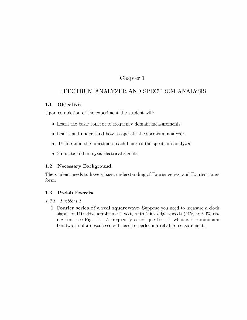
1.3.1 Problem 1
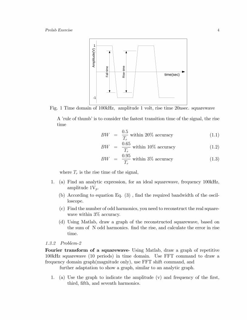
1. Fourier series of a real squarewave- Suppose you need to measure a clocksignal of 100 kHz, amplitude 1 volt, with 20ns edge speeds (10% to 90% ris-ing time see Fig. 1). A frequently asked question, is what is the minimumbandwidth of an oscilloscope I need to perform a reliable measurement.
Prelab Exercise 4
Am
plitu
de(V
)
time(sec)Fall
time
1
-1
Ris
etim
e
Fig. 1 Time domain of 100kHz, amplitude 1 volt, rise time 20nsec. squarewave
A �rule of thumb�is to consider the fastest transition time of the signal, the risetime
BW =0:5
Trwithin 20% accuracy (1.1)
BW =0:65
Trwithin 10% accuracy (1.2)
BW =0:95
Trwithin 3% accuracy (1.3)
where Tr is the rise time of the signal,
1. (a) Find an analytic expression, for an ideal squarewave, frequency 100kHz,amplitude 1Vp:
(b) According to equation Eq. (3) , �nd the required bandwidth of the oscil-loscope.
(c) Find the number of odd harmonics, you need to reconstruct the real square-wave within 3% accuracy.
(d) Using Matlab, draw a graph of the reconstructed squarewave, based onthe sum of N odd harmonics. �nd the rise, and calculate the error in risetime.
1.3.2 Problem-2
Fourier transform of a squarewave- Using Matlab, draw a graph of repetitive100kHz squarewave (10 periods) in time domain. Use FFT command to draw afrequency domain graph(magnitude only), use FFT shift command, and
further adaptation to show a graph, similar to an analytic graph.
1. (a) Use the graph to indicate the amplitude (v) and frequency of the �rst,third, �fth, and seventh harmonics.

References 5
1.3.3 Problem-3
Block diagram of a Spectrum Analyzer-Draw a block diagram of a spectrumanalyzer, and explain brie�y each of the following blocks (Attenuator,ampli�er,LPF,IF �lter, envelope detector, video �lter, display, LO, Ramp generator).
1.3.4 Problem-4
Shape factor of a Gaussian �lter-The voltage of a gaussian shape �lter is givenby
V (f) =1
�p2�exp
�(f � f0)
2
2�2
!(1.4)
where f0 is the center frequency of the �lter, and � is the standard deviation. Inprobability theory � is the standard deviation (About 68% of values drawn froma normal distribution are within one standard deviation, �). Electrical engineeringconsider the envelope of the curve.Assume that the the center frequency is 10MHz, and the -3dB bandwidth of the �lteris 1MHz.
1. (a) Use Eq. (4) to �nd the standart deviation of the �lter (-3dB is related tothe power V 2 (f) ).
(b) Use Eq. (4) to �nd the -60dB bandwidth of the �lter, and the shape factorof the �lter
Shape factor � �60dB Bandwidth�3dB Bandwidth
5 6 7 8 9 10 11 12 13 14 150.0
0.1
0.2
0.3
0.4
0.5
0.6
Frequencv(MHz)
-3dB
a
Ampl
itude
(V)
Figure problem 4
1.4 References
1. ROBERT A. WITTE "Spectrum and Network Measurements" . New Jersy ,Prentice Hall,1991
Background Theory -Frequency and Time Domain 6
2. CYDE F. COOMBS, Jr. "Electronic Instrument Handbook". McGraw-Hill, second edition 1995.
3. C. Rauscher: "Fundamental of Spectrum analysis" Rhode&Schwarz 2001.4. Agilent Company: "Spectrum Analysis Basics". Application Note 150,
January 2005.
1.5 Background Theory -Frequency and Time Domain
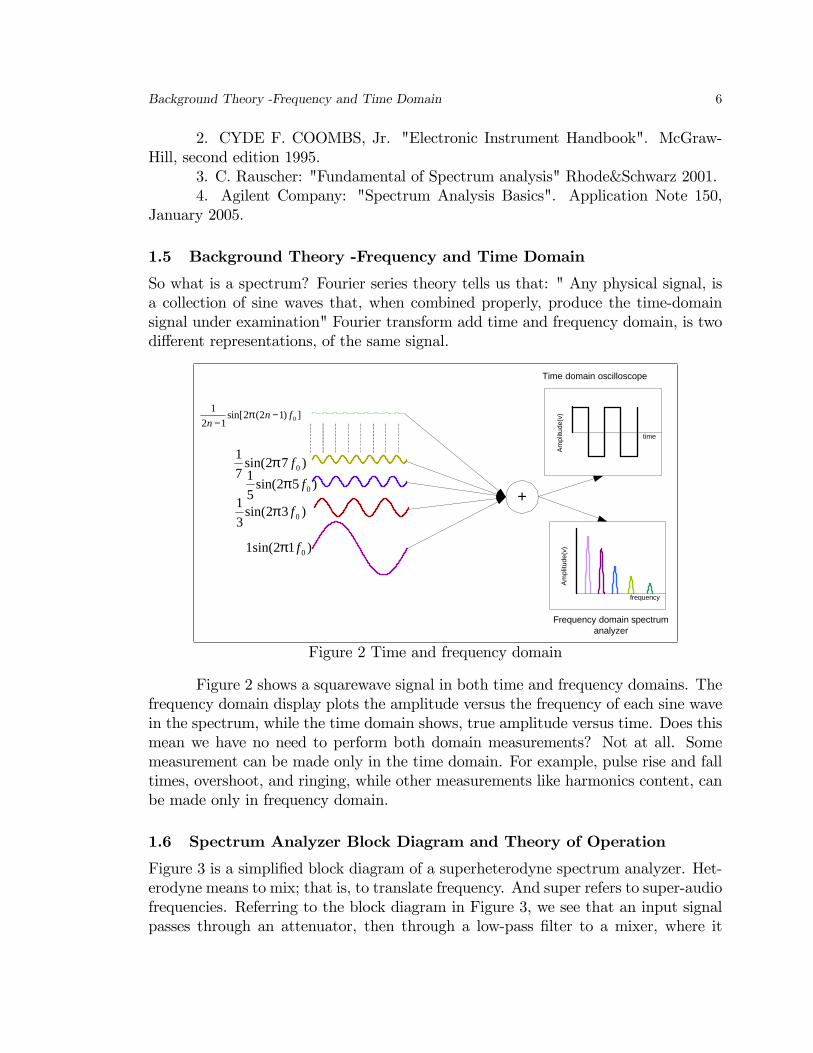
So what is a spectrum? Fourier series theory tells us that: " Any physical signal, isa collection of sine waves that, when combined properly, produce the time-domainsignal under examination" Fourier transform add time and frequency domain, is twodi¤erent representations, of the same signal.
time
Am
plitu
de(v
))12sin(1 0fπ
)32sin(31
0fπ
)52sin(51
0fπ
)72sin(71
0fπ
])12(2sin[12
10fn
n−
−π
+
Time domain oscilloscope
frequency
Ampl
itude
(v)
Frequency domain spectrumanalyzer
Figure 2 Time and frequency domain
Figure 2 shows a squarewave signal in both time and frequency domains. Thefrequency domain display plots the amplitude versus the frequency of each sine wavein the spectrum, while the time domain shows, true amplitude versus time. Does thismean we have no need to perform both domain measurements? Not at all. Somemeasurement can be made only in the time domain. For example, pulse rise and falltimes, overshoot, and ringing, while other measurements like harmonics content, canbe made only in frequency domain.
1.6 Spectrum Analyzer Block Diagram and Theory of Operation
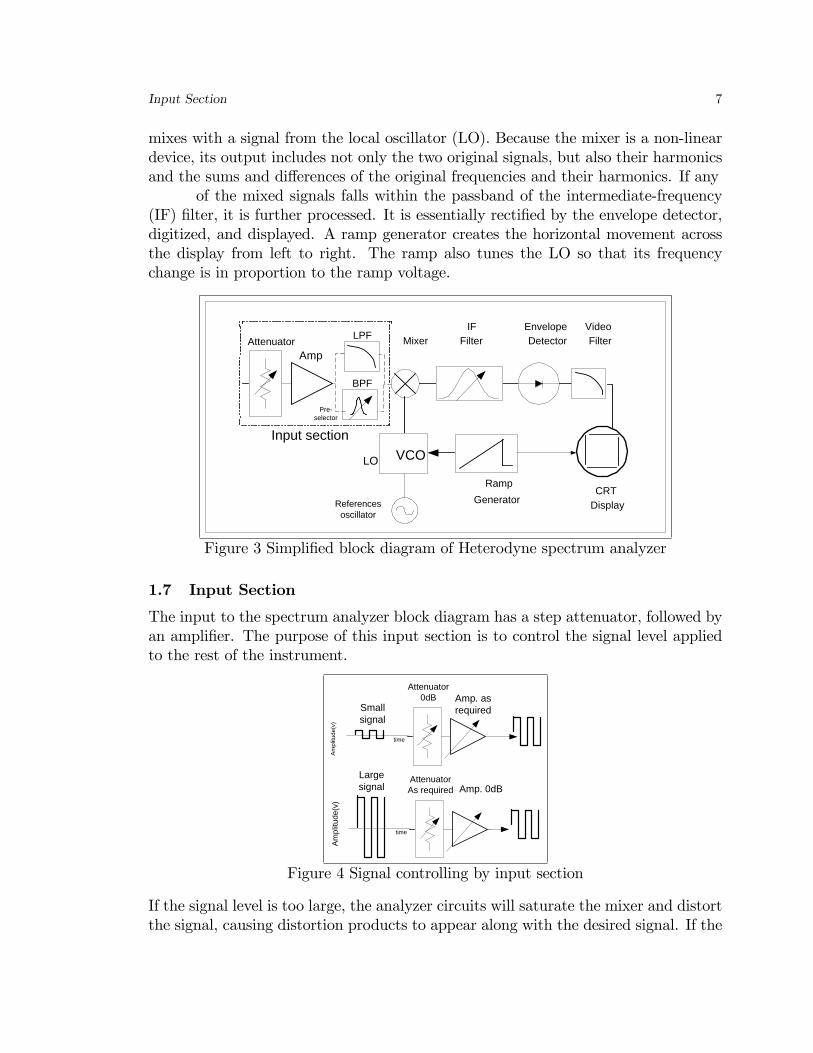
Figure 3 is a simpli�ed block diagram of a superheterodyne spectrum analyzer. Het-erodyne means to mix; that is, to translate frequency. And super refers to super-audiofrequencies. Referring to the block diagram in Figure 3, we see that an input signalpasses through an attenuator, then through a low-pass �lter to a mixer, where it
Input Section 7
mixes with a signal from the local oscillator (LO). Because the mixer is a non-lineardevice, its output includes not only the two original signals, but also their harmonicsand the sums and di¤erences of the original frequencies and their harmonics. If any
of the mixed signals falls within the passband of the intermediate-frequency(IF) �lter, it is further processed. It is essentially recti�ed by the envelope detector,digitized, and displayed. A ramp generator creates the horizontal movement acrossthe display from left to right. The ramp also tunes the LO so that its frequencychange is in proportion to the ramp voltage.
AttenuatorAmp
LPF MixerIF
FilterEnvelopeDetector
VideoFilter
CRTDisplay
RampGenerator
VCOLO
Input section
BPF
Pre-selector
Referencesoscillator
Figure 3 Simpli�ed block diagram of Heterodyne spectrum analyzer
1.7 Input Section
The input to the spectrum analyzer block diagram has a step attenuator, followed byan ampli�er. The purpose of this input section is to control the signal level appliedto the rest of the instrument.
time
Ampl
itude
(v)
Attenuator0dB Amp. as
requiredSmallsignal
time
Ampl
itude
(v)
AttenuatorAs required Amp. 0dB
Largesignal
Figure 4 Signal controlling by input section
If the signal level is too large, the analyzer circuits will saturate the mixer and distortthe signal, causing distortion products to appear along with the desired signal. If the
Mixer and Local oscillator. 8
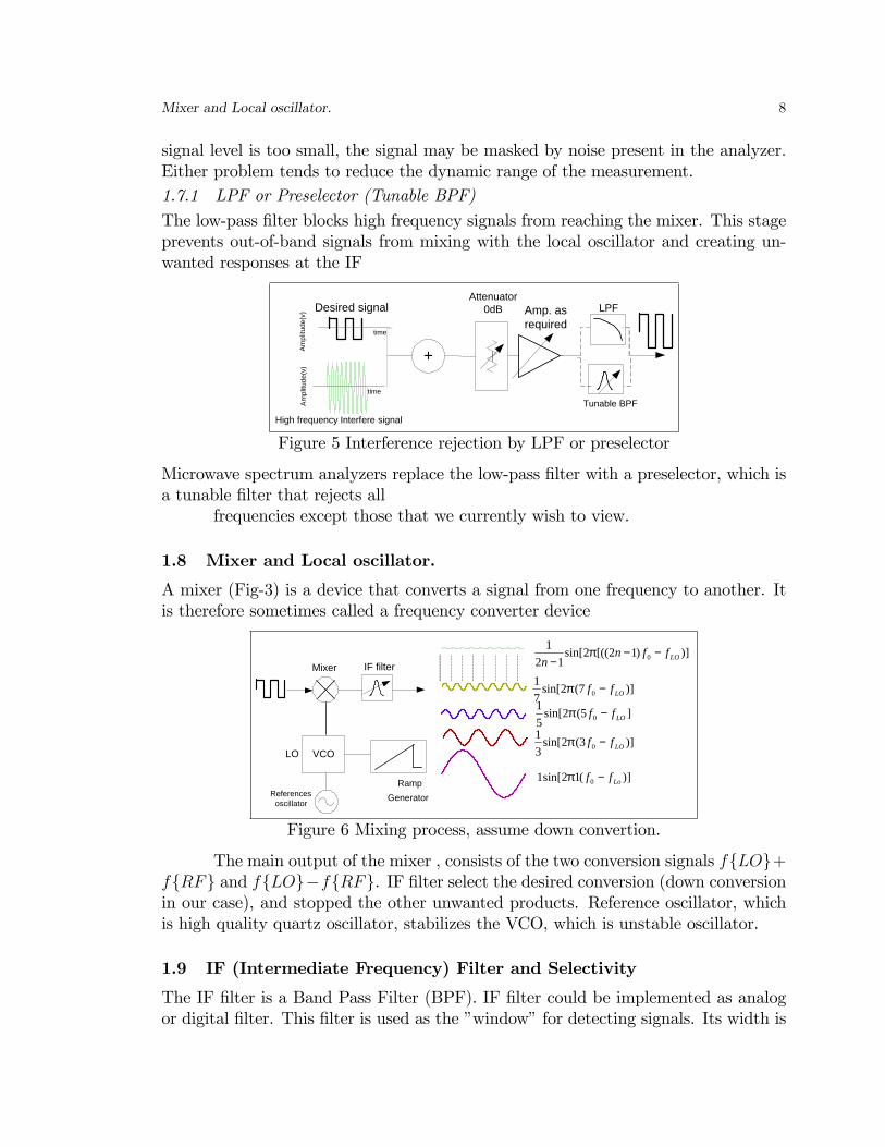
signal level is too small, the signal may be masked by noise present in the analyzer.Either problem tends to reduce the dynamic range of the measurement.1.7.1 LPF or Preselector (Tunable BPF)
The low-pass �lter blocks high frequency signals from reaching the mixer. This stageprevents out-of-band signals from mixing with the local oscillator and creating un-wanted responses at the IF
time
Am
plitu
de(v
) Desired signal
time
Am
plitu
de(v
)
High frequency Interfere signal
Attenuator0dB Amp. as
required
+
LPF
Tunable BPF
Figure 5 Interference rejection by LPF or preselector
Microwave spectrum analyzers replace the low-pass �lter with a preselector, which isa tunable �lter that rejects all
frequencies except those that we currently wish to view.
1.8 Mixer and Local oscillator.
A mixer (Fig-3) is a device that converts a signal from one frequency to another. Itis therefore sometimes called a frequency converter device
VCO
Mixer
LO
RampGenerator
IF filter
)](12sin[1 0 Loff −π
)]3(2sin[31
0 LOff −π
]5(2sin[51
0 LOff −π
)]7(2sin[71
0 LOff −π
)])12[((2sin[12
10 LOffn
n−−
−π
Referencesoscillator
Figure 6 Mixing process, assume down convertion.
The main output of the mixer , consists of the two conversion signals ffLOg+ffRFg and ffLOg�ffRFg. IF �lter select the desired conversion (down conversionin our case), and stopped the other unwanted products. Reference oscillator, whichis high quality quartz oscillator, stabilizes the VCO, which is unstable oscillator.
1.9 IF (Intermediate Frequency) Filter and Selectivity
The IF �lter is a Band Pass Filter (BPF). IF �lter could be implemented as analogor digital �lter. This �lter is used as the �window�for detecting signals. Its width is
Envelope detector 9
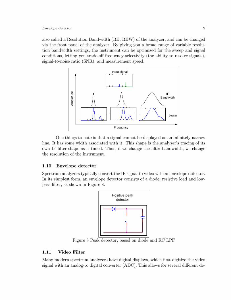
also called a Resolution Bandwidth (RB, RBW) of the analyzer, and can be changedvia the front panel of the analyzer. By giving you a broad range of variable resolu-tion bandwidth settings, the instrument can be optimized for the sweep and signalconditions, letting you trade-o¤ frequency selectivity (the ability to resolve signals),signal-to-noise ratio (SNR), and measurement speed.
-5
Input signal
IFBandwidth
Display
Frequency
Am
plot
ude
One things to note is that a signal cannot be displayed as an in�nitely narrowline. It has some width associated with it. This shape is the analyzer�s tracing of itsown IF �lter shape as it tuned. Thus, if we change the �lter bandwidth, we changethe resolution of the instrument.
1.10 Envelope detector
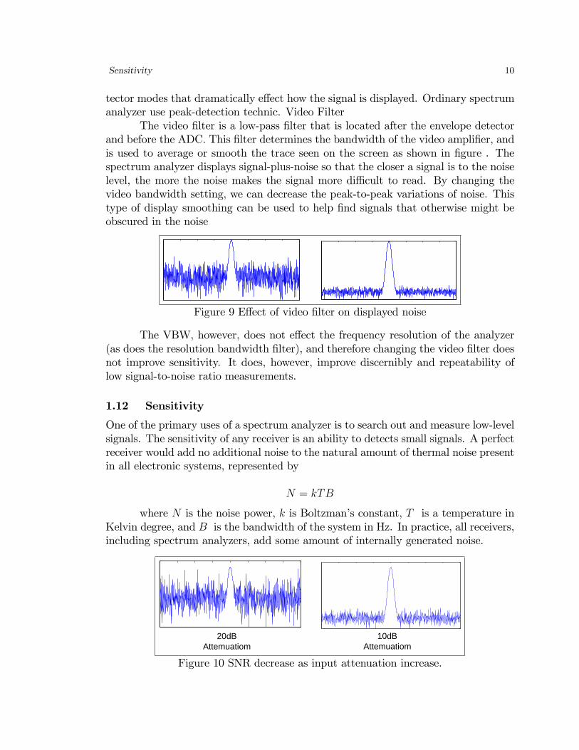
Spectrum analyzers typically convert the IF signal to video with an envelope detector.In its simplest form, an envelope detector consists of a diode, resistive load and low-pass �lter, as shown in Figure 8.
Positive peakdetector
Figure 8 Peak detector, based on diode and RC LPF
1.11 Video Filter
Many modern spectrum analyzers have digital displays, which �rst digitize the videosignal with an analog-to digital converter (ADC). This allows for several di¤erent de-
Sensitivity 10
tector modes that dramatically e¤ect how the signal is displayed. Ordinary spectrumanalyzer use peak-detection technic. Video Filter
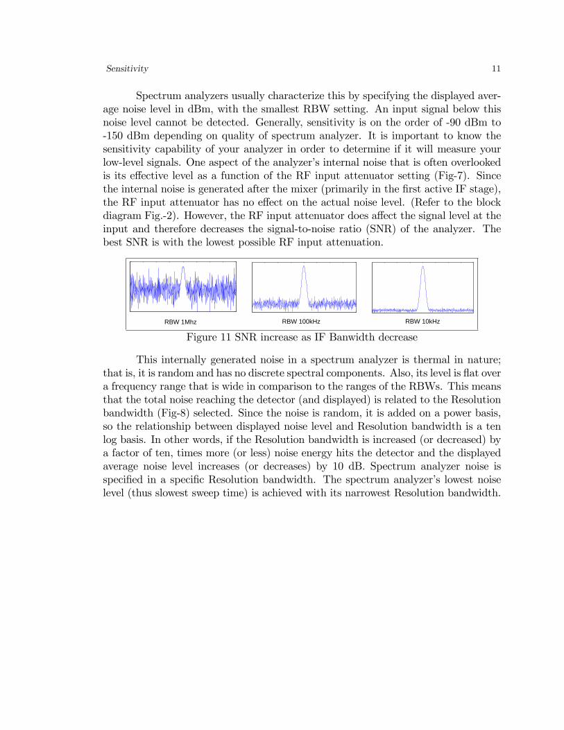
The video �lter is a low-pass �lter that is located after the envelope detectorand before the ADC. This �lter determines the bandwidth of the video ampli�er, andis used to average or smooth the trace seen on the screen as shown in �gure . Thespectrum analyzer displays signal-plus-noise so that the closer a signal is to the noiselevel, the more the noise makes the signal more di¢ cult to read. By changing thevideo bandwidth setting, we can decrease the peak-to-peak variations of noise. Thistype of display smoothing can be used to help �nd signals that otherwise might beobscured in the noise
Figure 9 E¤ect of video �lter on displayed noise
The VBW, however, does not e¤ect the frequency resolution of the analyzer(as does the resolution bandwidth �lter), and therefore changing the video �lter doesnot improve sensitivity. It does, however, improve discernibly and repeatability oflow signal-to-noise ratio measurements.
1.12 Sensitivity
One of the primary uses of a spectrum analyzer is to search out and measure low-levelsignals. The sensitivity of any receiver is an ability to detects small signals. A perfectreceiver would add no additional noise to the natural amount of thermal noise presentin all electronic systems, represented by
N = kTB
where N is the noise power, k is Boltzman�s constant, T is a temperature inKelvin degree, and B is the bandwidth of the system in Hz. In practice, all receivers,including spectrum analyzers, add some amount of internally generated noise.
20dBAttemuatiom
10dBAttemuatiom
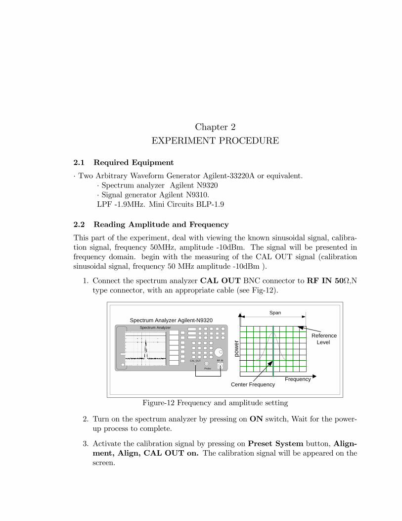
Figure 10 SNR decrease as input attenuation increase.
Sensitivity 11
Spectrum analyzers usually characterize this by specifying the displayed aver-age noise level in dBm, with the smallest RBW setting. An input signal below thisnoise level cannot be detected. Generally, sensitivity is on the order of -90 dBm to-150 dBm depending on quality of spectrum analyzer. It is important to know thesensitivity capability of your analyzer in order to determine if it will measure yourlow-level signals. One aspect of the analyzer�s internal noise that is often overlookedis its e¤ective level as a function of the RF input attenuator setting (Fig-7). Sincethe internal noise is generated after the mixer (primarily in the �rst active IF stage),the RF input attenuator has no e¤ect on the actual noise level. (Refer to the blockdiagram Fig.-2). However, the RF input attenuator does a¤ect the signal level at theinput and therefore decreases the signal-to-noise ratio (SNR) of the analyzer. Thebest SNR is with the lowest possible RF input attenuation.
RBW 10kHzRBW 100kHzRBW 1Mhz
Figure 11 SNR increase as IF Banwidth decrease
This internally generated noise in a spectrum analyzer is thermal in nature;that is, it is random and has no discrete spectral components. Also, its level is �at overa frequency range that is wide in comparison to the ranges of the RBWs. This meansthat the total noise reaching the detector (and displayed) is related to the Resolutionbandwidth (Fig-8) selected. Since the noise is random, it is added on a power basis,so the relationship between displayed noise level and Resolution bandwidth is a tenlog basis. In other words, if the Resolution bandwidth is increased (or decreased) bya factor of ten, times more (or less) noise energy hits the detector and the displayedaverage noise level increases (or decreases) by 10 dB. Spectrum analyzer noise isspeci�ed in a speci�c Resolution bandwidth. The spectrum analyzer�s lowest noiselevel (thus slowest sweep time) is achieved with its narrowest Resolution bandwidth.
Chapter 2
EXPERIMENT PROCEDURE
2.1 Required Equipment
� Two Arbitrary Waveform Generator Agilent-33220A or equivalent.� Spectrum analyzer Agilent N9320� Signal generator Agilent N9310.LPF -1.9MHz. Mini Circuits BLP-1.9
2.2 Reading Amplitude and Frequency
This part of the experiment, deal with viewing the known sinusoidal signal, calibra-tion signal, frequency 50MHz, amplitude -10dBm. The signal will be presented infrequency domain. begin with the measuring of the CAL OUT signal (calibrationsinusoidal signal, frequency 50 MHz amplitude -10dBm ).
1. Connect the spectrum analyzer CAL OUT BNC connector to RF IN 50;Ntype connector, with an appropriate cable (see Fig-12).
ReferenceLevel
Frequency
pow
er
Spectrum Analyzer Agilent-N9320
Center Frequency
Span
RF INCAL OUT
Spectrum Analyzer
Probe
Figure-12 Frequency and amplitude setting
2. Turn on the spectrum analyzer by pressing on ON switch, Wait for the power-up process to complete.
3. Activate the calibration signal by pressing on Preset System button, Align-ment, Align, CAL OUT on. The calibration signal will be appeared on thescreen.
Resolving Two Signals of Equal Amplitude 13
2.2.1 Setting the Reference Level and Center Frequency.
1. Press Amplitude, 10 dBm, what happen to the reference level? Press again0 dBm.
2. Press Frequency, 50 MHz, what happen to the center frequency?
2.2.2 Setting the Frequency Span.
1. Press SPAN, 50 MHz, what is the displayed, start frequency, and stopfrequency?
2.2.3 Using Marker to Read Frequency and Amplitude.
1. PressPeak Search, to place a marker (labeled-1) on the 50MHz signal peak.Note that the frequency and amplitude of the marker appear both in the activefunction block, and in the upper- right corner of the screen.
2.3 Resolving Two Signals of Equal Amplitude
In this example you explore the e¤ect of resolution bandwidth �lter (RBW), on theresolution of the spectrum analyzer, while measuring two signals of equal amplitude.2.3.1 Simulation of Resolving Two Signals of Equal Amplitude
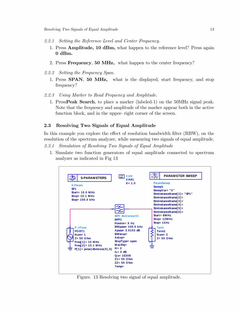
1. Simulate two function generators of equal amplitude connected to spectrumanalyzer as indicated in Fig 13
S_ParamSP1
Step= 100.0 kHzStop= 10.1 M HzStart= 10.0 M Hz
S-PARAM ETERSParamSweepSweep1
Step= 1kHzStop= 12M HzStart= 8M HzSimInstanceName[ 6] =SimInstanceName[ 5] =SimInstanceName[ 4] =SimInstanceName[ 3] =SimInstanceName[ 2] =SimInstanceName[ 1] = "SP1"SweepVar= "X"
PARAM ETER SWEEPVARVAR1X= 1.0
EqnVar
P_nTonePO RT1
P[ 1] = polar( dbmtow( 0) ,0)Freq[ 2] = 10.1 M HzFreq[ 1] = 10 M HzZ= 50 O hmNum= 1
BPF_ButterworthBPF1
Temp=Z2= 50 O hmZ1= 50 O hmQ u= 1E308IL= 0 dBN= 3M axRej=StopType= openAstop=BWstop=Apass= 3.0103 dBBWpass= 100.0 kHzFcenter= X Hz
TermTerm2
Z= 50 O hmNum= 2
Figure. 13 Resolving two signal of equal amplitude.
Resolving Two Signals of Equal Amplitude 14
2. Draw a graph of spectrum display, S21 versus variable X (center frequency),change the Y axis, to plot_vs(dB(max(S(2,1))), X), two signals are now visible.
3. Reduce BWpass of the �lter to 10kHz and watch the display.
4. Increase BWpass of the �lter to 300kHz and explain why one signals are nowvisible.
5. Explain if you change the order of the �lter, you improve the ability of spec-trum analyzer to resolve two signal of equal amplitude, prove your answer bysimulation.
2.3.2 Measurement of Resolving Two Signals of Equal Amplitude
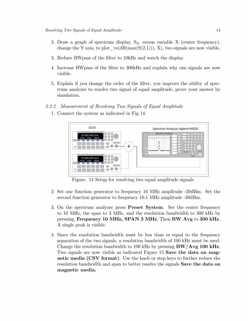
1. Connect the system as indicated in Fig 14.
+
Spectrum Analyzer Agilent-N9320
RF INCAL OUT
Spectrum Analyzer
Probe
20.000,000 kHzFreq Amp Offset
33220
20.000,000 kHzFreq Amp Offset
Figure. 14 Setup for resolving two equal amplitude signals
2. Set one function generator to frequency 10 MHz amplitude -20dBm. Set thesecond function generator to frequency 10.1 MHz amplitude -20dBm.
3. On the spectrum analyzer press Preset System. Set the center frequencyto 10 MHz, the span to 3 MHz, and the resolution bandwidth to 300 kHz bypressing, Frequency 10 MHz, SPAN 3 MHz, Then BW Avg to 300 kHz.A single peak is visible.
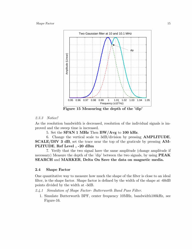
4. Since the resolution bandwidth must be less than or equal to the frequencyseparation of the two signals, a resolution bandwidth of 100 kHz must be used.Change the resolution bandwidth to 100 kHz by pressing BW/Avg 100 kHz.Two signals are now visible as indicated Figure 15 Save the data on mag-netic media (CSV format). Use the knob or step keys to further reduce theresolution bandwidth and span to better resolve the signals Save the data onmagnetic media.
Shape Factor 15
0.95 0.96 0.97 0.98 0.99 1 1.01 1.02 1.03 1.04 1.05Frequency (x107Hz)
Ampl
itude
(Lin
ear)
Two Gaussian filter at 10 and 10.1 MHz
dip
Figure 15 Measuring the depth of the �dip�
2.3.3 Notice!
As the resolution bandwidth is decreased, resolution of the individual signals is im-proved and the sweep time is increased.
5. Set the SPAN 1 MHz Then BW/Avg to 100 kHz.6. Change the vertical scale to 3dB/division by pressing AMPLITUDE,
SCALE/DIV 3 dB, set the trace near the top of the graticule by pressing AM-PLITUDE, Ref Level , -20 dBm
7. Verify that the two signal have the same amplitude (change amplitude ifnecessary) Measure the depth of the �dip�between the two signals, by using PEAKSEARCH andMARKER, Delta On Save the data on magnetic media.
2.4 Shape Factor
One quantitative way to measure how much the shape of the �lter is close to an ideal�lter, is the shape factor. Shape factor is de�ned by the width of the shape at -60dBpoints divided by the width at -3dB.
2.4.1 Simulation of Shape Factor- Butterworth Band Pass Filter.
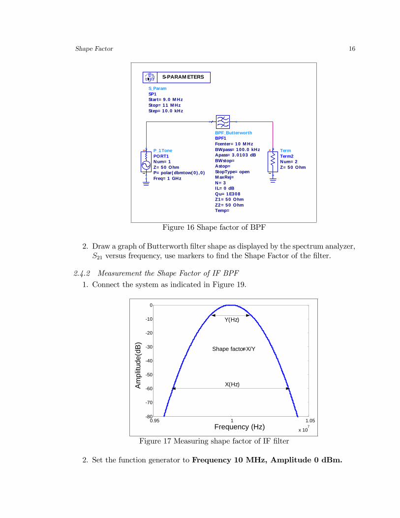
1. Simulate Butterworth BPF, center frequency 10MHz, bandwidth100kHz, seeFigure-16.
Shape Factor 16
P_1TonePORT1
Freq= 1 GHzP= polar( dbmtow( 0) ,0)Z= 50 OhmNum= 1
S_ParamSP1
Step= 10.0 kHzStop= 11 M HzStart= 9.0 M Hz
S-PARAM ETERS
BPF_ButterworthBPF1
Temp=Z2= 50 OhmZ1= 50 OhmQu= 1E308IL= 0 dBN= 3M axRej=StopType= openAstop=BWstop=Apass= 3.0103 dBBWpass= 100.0 kHzFcenter= 10 M Hz
TermTerm2
Z= 50 OhmNum= 2
Figure 16 Shape factor of BPF
2. Draw a graph of Butterworth �lter shape as displayed by the spectrum analyzer,S21 versus frequency, use markers to �nd the Shape Factor of the �lter.
2.4.2 Measurement the Shape Factor of IF BPF
1. Connect the system as indicated in Figure 19.
0.95 1 1.05
x 107
-80
-70
-60
-50
-40
-30
-20
-10
0
Frequency (Hz)
Am
plitu
de(d
B)
Shape factor=X/Y
X(Hz)
Y(Hz)
Figure 17 Measuring shape factor of IF �lter
2. Set the function generator to Frequency 10 MHz, Amplitude 0 dBm.
Measuring Signals using Logarithmic and Linear mode, Absolute and Relative Quantities. 17
3. Set the spectrum analyzer Frequency 10 MHz, Span 3 MHz, BW 100kHz, use the MARKER or MARKER Delta function, to �nd and recordthe -3 dB bandwidth of IF �lter.
4. Use the MARKER Delta function to measure the -60 dB bandwidth of theIF �lter, using the data calculate the shape factor (-60dB/-3dB bandwidth) ofthe 100 kHz BW �lter. Save the data on magnetic media (CSV format).
2.5 Measuring Signals using Logarithmic and Linear mode, Absoluteand Relative Quantities.
In this part of the experiment you measure the amplitude and frequency of the har-monics of 1 MHz Squarewave. The measurement will be in Absolute and Relativemode.
2.5.1 Simulation of a Squarewave in Frequency Domain
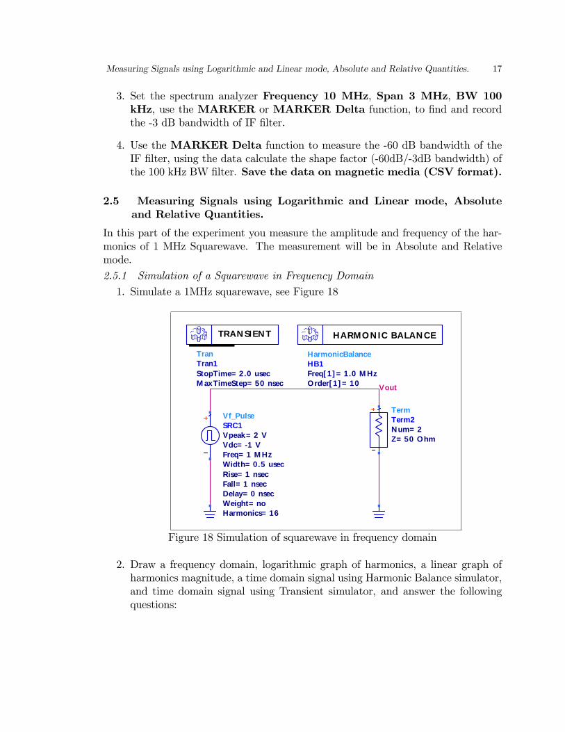
1. Simulate a 1MHz squarewave, see Figure 18
Vout
TranTran1
M axTimeStep= 50 nsecStopTime= 2.0 usec
TRAN SIEN T
HarmonicBalanceHB1
Order[ 1] = 10Freq[ 1] = 1.0 M Hz
HARMON IC BALAN CE
TermTerm2
Z= 50 OhmNum= 2
Vf_PulseSRC1
Harmonics= 16Weight= noDelay= 0 nsecFall= 1 nsecRise= 1 nsecWidth= 0.5 usecFreq= 1 M HzVdc= -1 VVpeak= 2 V
Figure 18 Simulation of squarewave in frequency domain
2. Draw a frequency domain, logarithmic graph of harmonics, a linear graph ofharmonics magnitude, a time domain signal using Harmonic Balance simulator,and time domain signal using Transient simulator, and answer the followingquestions:
Measuring Signals using Logarithmic and Linear mode, Absolute and Relative Quantities. 18
(a) Fill Table-1, and explain why the even harmonics disappear in linear mode
Absolute MeasurementHarmonics Frequency(MHz) Amplitude(dBm) Amplitude(mv)FirstSecondThird
Table -1
(b) Explain why the time domain squarewave graphs of the two simulator arenot identical?
2.5.2 Squarerave Measurement
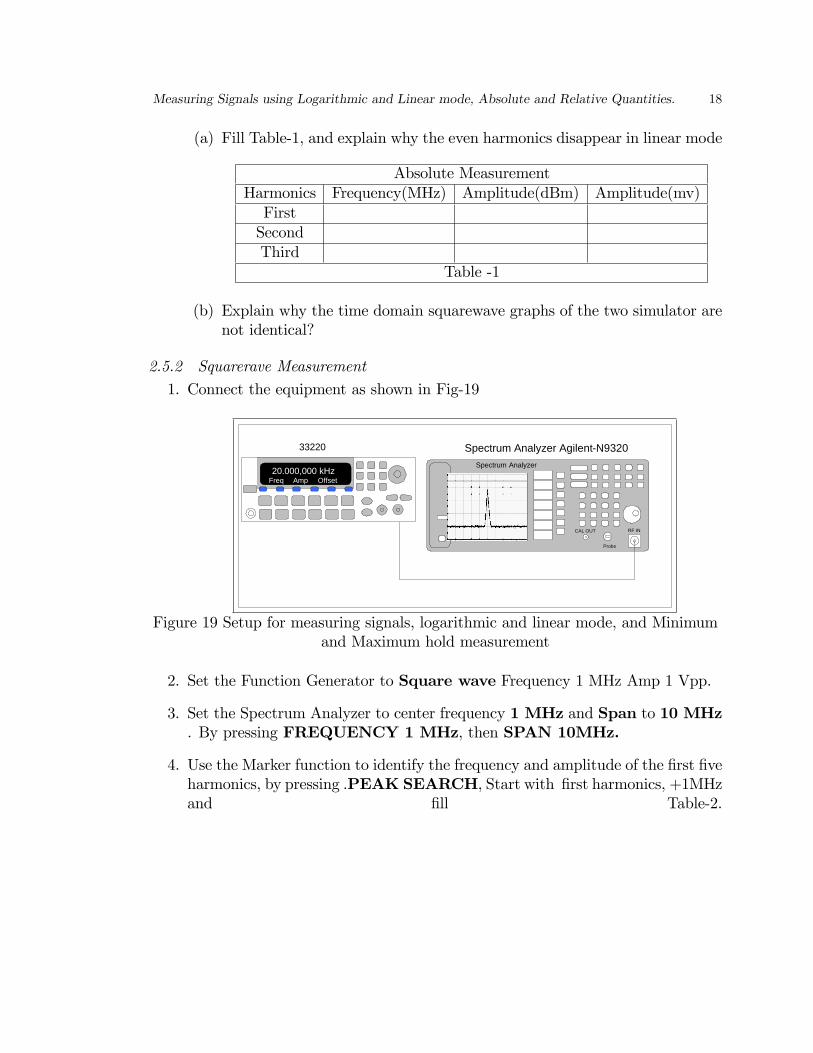
1. Connect the equipment as shown in Fig-19
Spectrum Analyzer Agilent-N9320
RF INCAL OUT
Spectrum Analyzer
Probe
20.000,000 kHzFreq Amp Offset
33220
Figure 19 Setup for measuring signals, logarithmic and linear mode, and Minimumand Maximum hold measurement
2. Set the Function Generator to Square wave Frequency 1 MHz Amp 1 Vpp.
3. Set the Spectrum Analyzer to center frequency 1 MHz and Span to 10 MHz. By pressing FREQUENCY 1 MHz, then SPAN 10MHz.
4. Use the Marker function to identify the frequency and amplitude of the �rst �veharmonics, by pressing .PEAK SEARCH, Start with �rst harmonics, +1MHzand �ll Table-2.
Measuring Frequency Response of LPF 19
Absolute MeasurementHarmonics Frequency(MHz) Amplitude(dBm) Amplitude(mv)FirstSecondThirdFourthFifth
Table -2
5. Measure the relative Amplitude and Frequency di¤erence between the odd har-monics, and �ll the relevant columns of Table -3. Compare the result to simu-lation. Save the data on magnetic media
Relative MeasurementHarmonics Frequency Amplitude Amplitude Matlab Simulation(No) di¤erence (MHz) di¤erence(dB) di¤erence(%) Result
First-ThirdThird-Fifth
Table -3
2.6 Measuring Frequency Response of LPF
The maximum hold function, can be powerful tool, while measuring frequency re-sponse of passive elements, such as LPF.2.6.1 Simulation of LPF
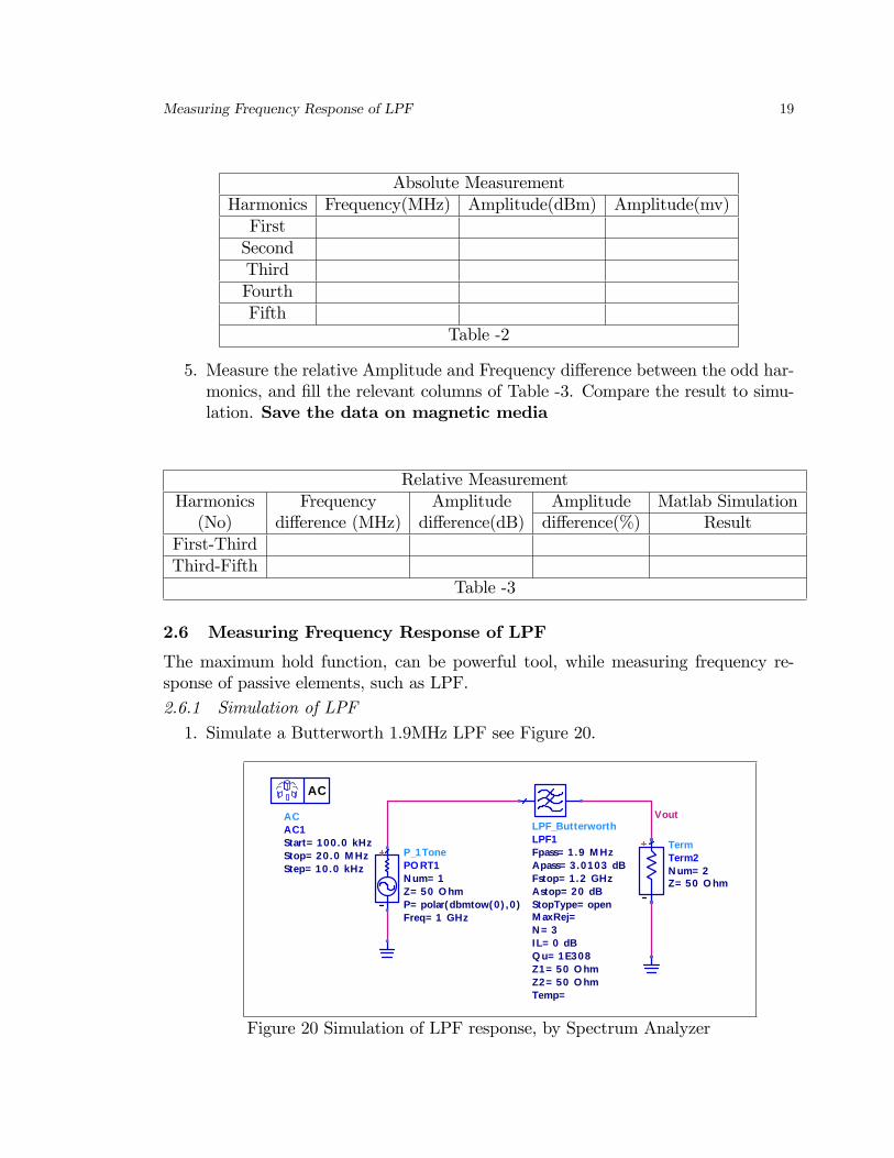
1. Simulate a Butterworth 1.9MHz LPF see Figure 20.
VoutACAC1
Step= 10.0 kHzStop= 20.0 M HzStart= 100.0 kHz
AC
P_1TonePO RT1
Freq= 1 GHzP= polar(dbmtow(0) ,0)Z= 50 O hmN um= 1
TermTerm2
Z= 50 O hmN um= 2
LPF_ButterworthLPF1
Temp=Z2= 50 O hmZ1= 50 O hmQ u= 1E308IL= 0 dBN = 3M axRej=StopType= openAstop= 20 dBFstop= 1.2 GHzApass= 3.0103 dBFpass= 1.9 M Hz
Figure 20 Simulation of LPF response, by Spectrum Analyzer
Measuring Frequency Response of LPF 20
2. Draw a graph of the �lter response, use marker delta function, to �nd thestopband slope of the �lter, dB/octave and dB/decade.
3. Explain if you increase the order of the �lter to N=5,the stopband slope of the�lter, dB/octave, decrease or increase? proove your answer by simulation.
2.6.2 Measurement of LPF
1. Add 1.9MHz Elliptic LPF to the input of the Spectrum Analyzer and connectthe equipment as shown in Figure 19.
2. Set the function generator to sweeper by setting, sweep mode, start frequency100Hz and stop frequency 10MHz. Press Sweep, Start 100Hz, Stop 10MHZ.
2.6.3 Setting the spectrum analyzer
In order to measure the frequency response of the LPF, we will use the maximumhold function, while the source is swept, and spectrum analyzer set to maximum holdthe trace.
1. PressPreset, Frequency, Center Freq, 1MHz, Span 10MHz, View/Trace,Max Hold.
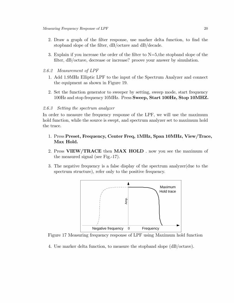
2. Press VIEW/TRACE then MAX HOLD . now you see the maximum ofthe measured signal (see Fig.-17).
3. The negative frequency is a false display of the spectrum analyzer(due to thespectrum structure), refer only to the positive frequency.
MaximumHold trace
Negative frequency Frequency0
Amp.
Figure 17 Measuring frequency response of LPF using Maximum hold function
4. Use marker delta function, to measure the stopband slope (dB/octave).
Measuring Signal To Noise Ratio of Low-Level Signal. 21
2.7 Measuring Signal To Noise Ratio of Low-Level Signal.
1. Connect the equipment as shown in Fig-16.
2. Set the function Generator to Sinewave, frequency 10 MHz, Output o¤.
3. Set the spectrum analyzer to 10 MHz Span 1 MHz. , by pressing Frequency,Center Freq, 10 MHz, Span 1 MHz. Can you explain why you see a signalwhile the output is o¤? .
4. Press BW/Avg , and Average On 50, to activate the trace average. Explainwhy the noise is changed under average, while the signal remain constant?
5. Measure the level of the signal (dBm), measure the level of the noise , andcalculate signal to noise ratio SNR, use marker delta to verify your calculation.Save the data on magnetic media
6. Increase the attenuation by 10dB, what happen to the SNR
7. Reduce the attenuation by 10dB, use marker to measure the level of the noise(under average). Decrease the BW, by factor 10, from 10kHz to 1 kHz andmeasure the level of the noise> Calculate the factor of noise level change.
2.8 Measuring a Signal Very Close to the Noise Floor
Spectrum analyzer sensitivity is the ability to measure low-level signals. It is limitedby the noise generated inside the spectrum analyzer. The spectrum analyzer inputattenuator, and bandwidth settings a¤ect the sensitivity, by changing the signal-to-noise ratio. The attenuator a¤ects the level of a signal passing through the instrument,whereas the bandwidth a¤ects the level of internal noise without a¤ecting the signal.If, after adjusting the attenuation and resolution bandwidth, a signal is still near thenoise, visibility can be improved by using the video-bandwidth and video-averagingfunctions.
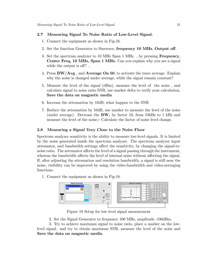
1. Connect the equipment as shown in Fig-18.
RF INCAL
Spectrum Analyzer
Probe
RF Iout
Signal Generator
LF out
AM
Mod
RF
600.000000 MHz
Figure 18 Setup for low level signal measurement
2. Set the Signal Generator to frequency 100 MHz, amplitude -100dBm.3. Try to achieve maximum signal to noise ratio, place a marker on the low-
level signal. and try to obtain maximum SNR. measure the level of the noise andSave the data on magnetic media.
Final Report 22
2.9 Final Report
1. Using the data of the �Resolving signals of equal amplitude�draw a graph ofthe two signals, and �nd the depth of the �dip�between the two signals, compareit to your measurement.
2. Draw a graph of the 1 MHz IF �lter, use the record data of the �lter, �ndthe Shape factor of the IF �lter. compare the calculated and measured Shapefactor.
3. Using the Measurement result of "Measuring Signal Very Close to the NoiseFloor", paragraph �nd the noise �gure of the spectrum analyzer
Noise Floor(dBm) = kTB (dBm) +NF (dB)