Embed Size (px)
Citation preview
ETH Library
Modulation techniques for theapplication of FTIR/DRIFTspectroscopy in heterogeneouscatalysis
Doctoral Thesis
Author(s):Ortelli, Enrico Eugenio
Publication date:2000
Permanent link:https://doi.org/10.3929/ethz-a-003913334
Rights / license:In Copyright - Non-Commercial Use Permitted
This page was generated automatically upon download from the ETH Zurich Research Collection.For more information, please consult the Terms of use.
Diss. ETH No 13694
Modulation Techniques for the
Application of FTIR/DRIFT Spectroscopy
in Heterogeneous Catalysis
A dissertation submitted to the
SWISS FEDERAL INSTITUTE OF TECHNOLOGY ZÜRICH
for the degree ofDoctor of Technical Sciences
Presented by
Enrico Eugenio Ortelli
dipl. Chem.-Ing. ETH
born the 3rd December 1971
citizen of Meride (TI)
accepted on the recommendation of
Prof. Dr. Alexander Wokaun, examiner
Prof. Dr. Alfons Baiker, co-examiner
Zürich 2000

This is page 2 !
This page was left intentionally blank !

G7h> f^cco^do del cawi waivm
o\Awa,j ^Jvomeo ed (çmwcco tyugwrda.

This is page 4 !
This page was left intentionally blank !
Acknowledgements
Acknowledgements
I would like to thank my advisor, Professor Dr. A. Wokaun, for stimulating discussions,
the continuous help and support during the time of my thesis. Without him, this work
would not have been possible.
I am also grateful to Professor Dr. A. Baiker for being my co-referee, and for making
available many of the catalyst samples investigated in this study.
I would like to thank Dr. J. Rritzenberger and Dr. J. Weigel-Meier for introducing me to
IR spectroscopy, and Dr. A. Bill for his assistance in the first FTIR experiments.
I would also like to thank Dr. J. Wambach for his friendly advice in the wide field of
heterogeneous catalysis.
I am grateful to Dr. D. Franzke, Dr. Th. Kunz, Dr. Ch. Hahn and Dr. T. Lippert for
stimulating discussions about science.
Particular thanks go to Dr. O. Haas, Dr. E. Newson, E. Uenala, F. Geiger, M. Kraus and
K. Geissler for their support and to P. Binkert, R. Hugi and Ch. Marmy for help with all
the mechanical and electronic problems.
Very special thank goes to my girlfriend, Marina, for her patience, continuing support,
love and confidence.
Finally, I would like to thank my parents for their understanding and support.
5
This is page 6 !
This page was left intentionally blank !
Ringraziamenti
Ringraziamenti
Desidero ringraziare il mio referente, Professor Dr. A. Wokaun, per le stimolanti
discussioni, il continuo aiuto e supporta durante tutto il mio dottorato. Senza di Lui
questo lavoro non sarebbe mai stato possibile.
Un grazie anche al Professor Dr. A. Baiker per vestire i panni del coreferente, e per aver
fornito gran parte dei catalizzatori utilizzati in questo studio.
Un ringraziamento anche al Dr. J. Kritzenberger e alia Dr.ssa J. Weigel-Meier per
avermi introdotto alia spettroscopia IR, nonchè al Dr. A. Bill per il suo aiuto durante la
prima parte degli esperimenti.
Desidero anche ringraziare il Dr. J. Wambach per i suoi sempre amichevoli consigli sul
vasto campo della catalisi eterogenea.
Un grazie anche al Dr. D. Franzke, Dr. Th. Kunz, Dr.ssa Ch. Hahn e Dr. T. Lippert per
le stimolanti discussioni nel campo scientifico.
Un grazie particolare al Dr. O. Haas, Dr. E. Newson, E. Uenala, F. Geiger, M. Kraus e
K. Geissler per il loro sostegno; e a P. Binkert, R. Hugi e Ch. Marmy per il sempre
pronto aiuto nel risolvere i vari problemi sia di ordine meccanico che elettronico.
Un ringraziamento veramente speciale va alla mia ragazza, Marina, per la sua pazienza,
il continuo supporta, l'amore e la fiducia sempre presenti.
In ultimo, vorrei ringraziare i miei genitori per la comprensione e il supporto
dimostratomi.
7
This is page 8 !
This page was left intentionally blank !
Table of contest
Table of contest
Acknowledgements 5
Ringraziamenti 7
Table of contest 9
Summary 15
Riassunto 17
Zusammenfassung 19
1. Introduction 21
1.1 Infrared spectroscopy 21
1.1.1 Definitions 21
1.1.2 Brief history of IR spectroscopy 23
1.2 Fourier transform IR spectroscopy 24
1.2.1 Introduction of the Fourier transform in the IR spectroscopy 24
1.2.2 Michelson interferometer and Fourier transform 26
1.3 Diffuse reflectance 27
1.3.1 Definitions 27
1.3.2 Specular reflectance 28
1.3.3 Diffuse reflectance 29
1.3.4 Parameters affecting the DRIFT spectrum 30
1.3.5 Gas phase species in DRIFT spectroscopy 31
1.4 DRIFT in heterogeneous catalysis 32
1.4.1 Introduction of DRIFT in heterogeneous catalysis 32
1.4.2 Use of DRIFT in heterogeneous catalysis 33
1.5 Scope ofthis thesis 33
2. Experimental 35
Table of contest
2.1 The experimental setup 35
2.2 The controlprogram 36
2.2.1 The programming language: LabVIEW 36
2.2.2 The control program 37
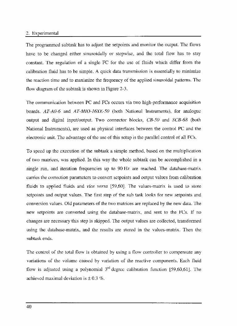
2.2.3 Management of the mass flow controllers {measure FCs) 39
2.2.4 Management of the temperature controllers {measure TCs) 41
2.2.5 The triggering of the spectrometer {trigger IFS) 42
2.3 The gas dosing systems 44
2.3.1 The Preparative Unit 44
2.3.2 The Modulation Unit 46
2.4 DRIFT: optical accessories and methodic 48
2.4.1 Controlled Environmental Chamber 48
2.4.2 Environmental Chamber 49
2.4.3 Representation of DRIFT spectra 50
2.4.4 Sample preparation 51
2.5 The micro reactor I gas cell system 51
2.6 The FTIR spectrometer 53
2.6.1 The instrument 53
2.6.2 The macro 53
2.7 Catalytic tests 55
2.8 Compounds 56
3. Reactants modulation 57
3.1 Introduction 57
3.2 Approach to the problem 59
3.3 Modulation ofthe reactants 60
3.3.1 Mathematical background 60
3.3.2 Modelling the setup 62
3.3.3 Experimental procedure 63
3.3.4 Experimental parameters 65
3.3.4.1 Determination oftdeiay 65
3.3.4.2 Delay element of 1st Order (PTi) 66
3.3.4.3 Delay element of2nd Order (PT2) 68
3.3.5 Recording techniques 72
3.3.6 Recording parameters 73
3.4 Useful simple models 74
3.4.1 A few definitions in heterogeneous catalysis 74
3.4.2 Heterogeneous reactions in the used setup 75
3.4.2.1 Adsorption/desorption equilibrium 76
10
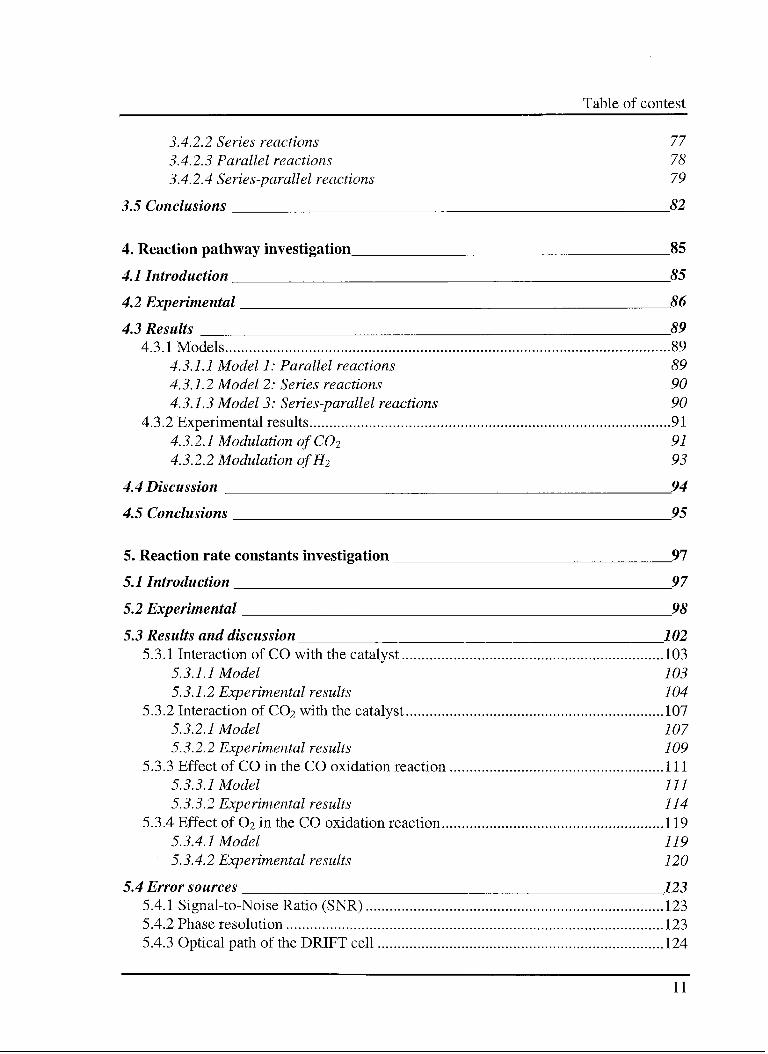
Table of contest
3.4.2.2 Series reactions 77
3.4.2.3 Parallel reactions 78
3.4.2.4 Series-parallel reactions 79
3.5 Conclusions 82
4. Reaction pathway investigation 85
4.1 Introduction 85
4.2 Experimental 86
4.3 Results 89
4.3.1 Models 89
4.3.1.1 Model 1: Parallel reactions 89
4.3.1.2 Model 2: Series reactions 90
4.3.1.3 Model 3: Series-parallel reactions 90
4.3.2 Experimental results 91
4.3.2.1 Modulation of C02 91
4.3.2.2 Modulation ofR2 93
4.4 Discussion 94
4.5 Conclusions 95
5. Reaction rate constants investigation 97
5.1 Introduction 97
5.2 Experimental 98
5.3 Results and discussion 102
5.3.1 Interaction of CO with the catalyst 103
5.3.1.1 Model 103
5.3.1.2 Experimental results 104
5.3.2 Interaction of C02 with the catalyst 107
5.3.2.1 Model 107
5.3.2.2 Experimental results 109
5.3.3 Effect of CO in the CO oxidation reaction Ill
5.3.3.1 Model 111
5.3.3.2 Experimental results 114
5.3.4 Effect of 02 in the CO oxidation reaction 119
5.3.4.1 Model 119
5.3.4.2 Experimental results 120
5.4 Error sources 123
5.4.1 Signal-to-Noise Ratio (SNR) 123
5.4.2 Phase resolution 123
5.4.3 Optical path of the DRIFT cell 124
11
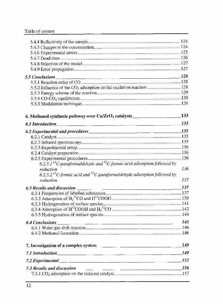
Table of contest
5.4.4 Reflectivity of the sample 124
5.4.5 Changes in the concentration 124
5.4.6 Experimental errors 125
5.4.7 Dead time 126
5.4.8 Selection of the model 127
5.4.9 Error propagation 127
5.5 Conclusions 128
5.5.1 Reaction order of CO 128
5.5.2 Influence of the C02 adsorption on the oxidation reaction 128
5.5.3 Energy scheme of the reaction 129
5.5.4 CO-C02 equilibrium 130
5.5.5 Modulation technique 131
6. Methanol synthesis pathway over Cu/Zr02 catalysts 133
6.1 Introduction 133
6.2 Experimental andprocedures 135
6.2.1 Catalyst 135
6.2.2 Infrared spectroscopy 135
6.2.3 Experimental setup 136
6.2.4 Catalyst preparation 136
6.2.5 Experimental procedures 136
6.2.5.1 C-paraformaldehyde and C-formic acid adsorptionfollowed by
reduction 1367 ? 79
6.2.5.2 C-formic acid and C-paraformaldehyde adsorptionfollowed by
reduction 137
6.3 Results and discussion 137
6.3.1 Frequencies of labelled substances 137
6.3.2 Adsorption of H213CO and H12COOH 139
6.3.3 Hydrogénation of surface species 141
6.3.4 Adsorption of H13COOH and H212CO 142
6.3.5 Hydrogénation of surface species 144
6.4 Conclusions 145
6.4.1 Water gas shift reaction 146
6.4.2 Methanol formation 146
7. Investigation of a complex system 149
7.1 Introduction 149
7.2 Experimental 152
7.3 Results and discussion 156
7.3.1 C02 adsorption on the reduced catalyst 157
12
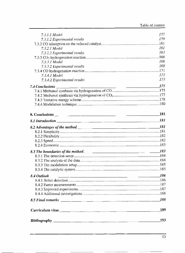
Table of contest
7.3.1.1 Model 157
7.3.1.2 Experimental results 159
7.3.2 CO adsorption on the reduced catalyst 161
7.3.2.1 Model 161
7.3.2.2 Experimental results 163
7.3.3 C02 hydrogénation reaction 166
7.3.3.1 Model 166
7.3.3.2 Experimental results 168
7.3.4 CO hydrogénation reaction 171
7.3.4.1 Model 171
7.3.4.2 Experimental results 173
7.4 Conclusions 175
7.4.1 Methanol synthesis via hydrogénation of CO 175
7.4.2 Methanol synthesis via hydrogénation of CQ2 177
7.4.3 Tentative energy scheme 178
7.4.4 Modulation technique 180
8. Conclusions 181
8.1 Introduction 181
8.2 Advantages ofthe method 181
8.2.1 Simplicity 181
8.2.2 Flexibility 182
8.2.3 Speed 182
8.2.4 Economic 183
8.3 The boundaries ofthe method 183
8.3.1 The detection setup 184
8.3.2 The analysis of the data 184
8.3.3 The modulation setup 185
8.3.4 The catalytic system 185
8.4 Outlook 186
8.4.1 Better detection 186
8.4.2 Faster measurements 187
8.4.3 Improved experiments 187
8.4.4 Additional investigations 188
8.5 Final remarks 188
Curriculum vitae 189
Bibliography 193
13
This is page 14 !
This page was left intentionally blank !
Summary
Summary
In this work a new experimental method based on FTIR and DRIFT spectroscopy has
been presented. The method is applicable to both qualitative and quantitative
measurements in heterogeneous catalysis. The basis of the modulation theory, its
advantages, limitations, possible improvements, and several examples are discussed.
The necessary setup consists of the same components as used in standard studies of
heterogeneously catalysed reactions, and includes mainly commercial parts.
The method is based on the idea that, from the analysis of the transformation of an input
perturbation signal into a response signal, information about the investigated system can
be obtained. Sinusoidal modulation of the reactant concentrations is chosen as the
perturbation, which allows one to monitor the concomitant changes in the
concentrations of different intermediates and products along the reaction pathway.
For quantitative measurements, the use of sinusoidal shaping of the modulation has the
advantage that calibration curves (FTIR spectroscopy) and ad hoc mathematical models
for the variation of the reflectivity of the used catalyst (DRIFT spectroscopy) are
unnecessary. Several parameters are collected at the same time during a single
measurement. The accumulated data provide information about the different
characteristics of the investigated system, from which other kinetic and thermodynamic
parameters can be derived.
The four essential components of a modulation experiment are the catalytic system, the
modulation setup, the detection system, and the data analysis algorithms. These
components are closely related to each other, and each characterised by a set of
operating parameters. To achieve the optimum working conditions, all possible
15
Summary
parameters must be considered and tested. Extended test experiments have been carried
out for this purpose.
The following reactions have been studied.
1. Reaction pathway investigation. As a test reaction, the methanol synthesis from
CO/C02/H2 over a commercial Cu/ZnO/Al203 catalyst was used. The investigation was
performed using FTIR spectroscopy and possible reaction pathways were discussed in
terms of standard chemical reaction engineering models. The modulation data were
found to be represented by a set of series and parallel reactions.
2. Reaction rate constants investigation. The CO oxidation over a Pd25Zr75 based
catalyst was studied in detail using DRIFT spectroscopy. Reaction rate constants as well
as the rate limiting step were determined. The repetition of the experiments at different
temperatures allowed the calculation of the activation energies of different reaction
steps, as well as modelling the conversion in the corresponding catalytic tests.
3. Investigation of a complex system. The application of the modulation concept to
study in situ (DRIFT) the reaction pathway and the reaction rate constants of a complex,
solid-state catalysed reaction system is described. The methanol synthesis over a
Cu4ôZr54 based catalyst starting from H2/CO and H2/C02 was chosen as test reaction.
Reaction rate constants as well as activation energies of the different reaction steps were
determined.
16
Riassunto
Riassunto
In questo lavoro viene presentato un nuovo metodo sperimentale applicato alia
spettroscopia FTIR e DRIFT, sia per ricerche quantitative che qualitative nel campo
délia catalisi eterogenea. Le basi del metodo, i vantaggi, i limiti, le possibili migliorie
come pure diversi esempi di applicazione vengono riportati e discussi. Le infrastrutture
e le apparecchiature necessarie per eseguire gli esperimenti sono le medesime che si
usano per conduire normali ricerche in catalisi eterogenea.
II metodo è basato sulla semplice idea che ogni azione induce una reazione, pertanto
analizzando come reagisce un sistema che viene perturbato da un segnale definito, si
possono ottenere informazioni sul sistema stesso. Modulando sinusoidalmente la
concentrazione dei reattandi si ottiene un'oscillazione indotta nelle concentrazioni dei
diversi composti intermedi cosi come dei prodotti.
L'uso di curve sinusoidali élimina la nécessita di creare delle curve di calibrazione
(spettroscopia FTIR) come pure l'elaborazione di modelli matematici ad hoc che
tengano conto delle variazioni délia reflettività del catalizzatore usato (spettroscopia
DRIFT). Durante la medesima misurazione, diversi parametri sono raccolti alio stesso
momento. Questi forniscono, da un lato, informazioni sulle differenti caratteristiche del
sistema, dall'altro sono usati per ricavare dati riguardanti i processi cinetici come pure le
caratteristiche termodinamiche del sistema stesso.
I quattro gruppi di elementi che limitano il sistema sono: il sistema di detezione, l'analisi
dei dati, il dosaggio dei gas e il sistema catalitico. Dato che questi s'influenzano l'un
l'altro, per ottenere le condizioni ideali di sperimentazione è necessario considerare tutti
i possibili parametri. L'esecuzione di esperimenti per testare l'influsso dei vari parametri
puö diventare un processo lungo e impegnativo.
17
Riassunto
Gli esempi di applicazione presentati sono i seguenti.
1. Classificazione del meccanismo di reazione. Corne reazione è stata scelta la
sintesi del metanolo partendo da CO/C02/H2 su un catalizzatore commerciale
Cu/ZnO/Al203. La spettroscopia FTIR viene utilizzata per ottenere delle informazioni
sui possibili meccanismi di reazione. I dati raccolti sono discussi basandosi sui modelli
standard usati nel campo del genio chimico. Nel caso considerato viene dimostrata
l'esistenza di reazioni in parallelo e in série.
2. Studio sulle costanti di reazione. L'ossidazione del CO su un catalizzatore
Pd25Zr75 viene analizzata in dettaglio usando la spettroscopia DRIFT. I dati raccolti
vengono usati per determinare le velocità di reazione dalle quali si ottiene poi la
reazione limitante. La ripetizione deU'esperimento a diverse temperature fornisce la
possibilità di stimare l'energia di attivazione delle differenti reazioni presenti nonchè la
conversione.
3. Studio di un sistema catalitico complesso. Il concetto di modulazione viene
applicato ad un sistema complesso quale la sintesi del metanolo su un catalizzatore
Cu4ôZr54 partendo da CO/C02/H2. Il sistema viene analizzato in situ (DRIFT) al fine di
ottenere informazioni sui meccanismi di reazione e sulle velocità di reazione, queste
sono poi usate per stimare l'energia di attivazione delle differenti reazioni.
18
Zusammenfassung
Zusammenfassung
In dieser Arbeit wird eine neue experimentelle Methode präsentiert, die auf FTIR- und
DRIFT-Spektroskopie basiert. Die Methode kann benutzt werden, um qualitative sowie
quantitative Untersuchungen in der heterogenen Katalyse durchzuführen. Die Theorie
der Modulationstechnik, Vorteile, Begrenzungen, mögliche Verbesserungen sowie
Anwendungsbeispiele werden vorgestellt. Der notwendige Aufbau besteht aus ähnlichen
Komponenten, wie sie bei Standarduntersuchungen in der heterogenen Katalyse
eingesetzt werden.
Die Methode basiert auf der einfachen Idee, dass aus der Analyse der Umwandlung
eines Störsignal in ein Antwortsignal Informationen über das untersuchte System
erhalten werden können. Als Störsignal wird die sinusförmige Modulation der
Konzentration eines der Edukte benutzt, so dass die dadurch verursachte Änderung der
verschiedenen Zwischen- und Endprodukte beobachtet werden kann.
Der Einsatz von sinusförmiger Modulation eignet sich besonders für quantitative
Analysen, da man auf Eichkurven (FTIR Spektroskopie) oder ad hoc entwickelte
mathematische Modelle (DRIFT Spektroskopie), welche die optischen Eigenschaften
des untersuchten Katalysators voraussetzen, verzichten kann. Weiterhin werden
gleichzeitig mehrere Kenngrössen erhalten. Aus den Daten werden Informationen über
die verschiedenen Eigenschaften des untersuchten System gewonnen, aus denen weitere
kinetische und thermodynamische Parameter abgeleitet werden.
Die vier wesentlichen Komponenten des Experimentes sind die Beaufschlagung des
katalytischen Systems, die Vorbereitung und Modulation der Feedgas-Konzentration,
das Detektions-system und die Analyse der Daten. Diese beeinflussen sich gegenseitig,
weswegen alle möglichen Parameter betrachtet werden sollen, um ideale
19
Zusammenfassung
Reaktionsbedingungen zu finden. Zu diesem Zweck wurden eingehende Testmessungen
durchgeführt.
Die folgenden Reaktionen wurden untersucht.
1. Klassifizierung des Reaktionsmechanismus. Als Test-Reaktion wurde die
Methanol Synthese aus CO/C02/H2 über einen kommerziellen Cu/ZnO/Al203
Katalystor benutzt. FTIR-Spektroskopie wurde angewendet, um Informationen über
mögliche Reaktionsmechanismen zu erhalten. Die Resultate wurden im Rahmen von
Standard-Modellen der chemischen Reaktionstechnik diskutiert und lieferten im
vorliegenden Fall Evidenz für das simultane Ablaufen von seriellen und parallelen
Reaktionen.
2. Bestimmung von Reaktionsgeschwindigkeitskonstanten. Die CO-Oxidation über
einem Pd25Zr75-basierten Katalysator wurde mit DRlb'l-Spektroskopie im Detail
studiert. Die Reaktionsgeschwindigkeitskonstanten und der geschwindigkeits-
limitierende Schritt konnte ermittelt werden. Durch Experimente bei verschieden
Temperaturen wurden die Aktivierungsenergien der verschiedenen Schritte bestimmt
und der Umsatz in den entsprechenden katalytischen Experimenten modelliert.
3. Untersuchung eines komplexeren katalytische Systems. Das Modulationskonzept
wurde zur Untersuchung des Reaktionsmechanismus der Methanolsynthese aus H2/CO
und H2/C02 über einen Cu4öZr54 Katalysator verwendet. Die Reaktionsgeschwindig¬
keitskonstanten und die Aktivierungsenergien der verschiedenen Reaktionsschritte
wurden bestimmt.
20
1.1 Infrared spectroscopy
1. Introduction
1.1 Infrared spectroscopy
1.1.1 Definitions
Infrared spectroscopy (from Latin spectrum = the appearance and from Greek
skopein = to view) is defined as the use of instrumentation in measuring a physical
property of matter, and the relating of the obtained data to the chemical composition.
The measured physical property of the matter is the ability of absorption, transmission
or reflection of infrared radiation. The analysis of the radiation gives information about
the identity, the quantity, the structure, and the environment of molecules as well as
ions.
Not all forms of matter are capable of producing an infrared spectrum (i. e. metals do
not). To give rise to the absorption bands appearing in the spectrum the infrared
radiation has to interact with vibrational (and rotational) excitations of the molecule. In
contrast to pure rotational (microwave) spectroscopy, a permanent dipole moment is not
required in vibrational spectroscopy. However, only those vibrations involving a dipole
momentum that changes its intensity {dM) during the bond excursion (dq) are infrared
active.
*o (i.i)dq
21
1. Introduction
Example: methane (CH4) has M = 0 but several vibrations with dM/dq ^ 0.
Vibrations may involve the modification of bond lengths -stretching- or of the bond
angles -deformation-, or relative torsional motions of molecular moieties. The intensity
of the infrared radiation {IRBand) is proportional to the square of the change of the dipole
momentum as function of the interatomic distance (dr) [1].
IRBand °=
'dM^
[. dr J(1.2)
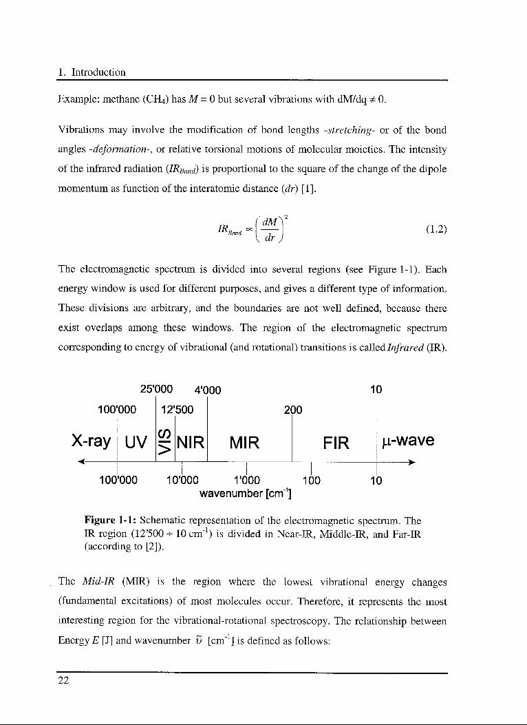
The electromagnetic spectrum is divided into several regions (see Figure 1-1). Each
energy window is used for different purposes, and gives a different type of information.
These divisions are arbitrary, and the boundaries are not well defined, because there
exist overlaps among these windows. The region of the electromagnetic spectrum
corresponding to energy of vibrational (and rotational) transitions is called Infrared (IR).
25'CIOO 4'000
100'OQO
X-ray UV
12'500
NIRCO
>
10
200
MIR FIR
ioo'ooo lo'ooo rooo 100
wavenumber [cm1]10
iu-wave
—
Figure 1-1: Schematic representation of the electromagnetic spectrum. The
IR region (12'500 * 10 cm"1) is divided in Near-IR, Middle-IR, and Far-IR
(according to [2]).
The Mid-IR (MTR) is the region where the lowest vibrational energy changes
(fundamental excitations) of most molecules occur. Therefore, it represents the most
interesting region for the vibrational-rotational spectroscopy. The relationship between
Energy E [J] and wavenumber v [cm-1] is defined as follows:
22
1.1 Infrared spectroscopy
E = he 100 v (1.3)
where c is the speed of the light and h the Planck's constant (6.626-10"34 J s). The
wavenumber ö as a function of the wavelength X [m] is given by the following
equation.
v=—^— (1.4)100 À
1.1.2 Brief history of IR spectroscopy
The basis for the development of the spectroscopy was originated several billion of
years ago with the creation of the light {And God said: Eet there be light'. - Genesis 1;3)
and its composition {I set my bow in the clouds, and it shall be a sign, - Genesis 9; 13).
Several centuries ago humans recognised that light is necessary for colours to exist
(Aristotele, 400 BC), and, after two millennia, that it can be divided into a spectrum
(Newton, Principia, 1666). In 1678 Huygens proposed the wave theory of light. This
was validated in 1802 by Thomas Young, who obtained the spectrum of light by
diffraction using a crude transmission grating. In 1860 J. C. Maxwell developed the
mathematical equations describing the light as an electromagnetic wave.
In 1800 F. W. Herschel noted that different amounts of heat passed through distinct
coloured glasses. He hence deduced that heat is similar to light. In 1900 William
Coblentz collected the first IR spectra of organic compounds. In 1949 John White and
Max Listen developed the double-beam optical zero adjustment IR spectrometer. With
the commercialisation of this system the chemical infrared spectroscopy came into
widespread use. These dispersive instruments proved the tremendous importance of
infrared analysis which soon became the characterisation workhorse in chemical
laboratories.
23
1. Introduction
The mathematical equation describing the attenuation of a wave passing through a
sample was found in 1760 by Johann Lambert. His starting point were the experiments
of Pierre Bouger (1729), who noticed the attenuation of light as it passed through
successive thicknesses of glass. In 1852 August Beer showed the logarithmic relation of
the Bouguer-Lambert Law. The Bouger-Lambert-Beer Equation (see Equation 1.5)
describes the attenuation dl of a radiation having a wavelength À through a sample with
a concentration c and natural extinction coefficient £n {A) as function of the sample
thickness dl.
% = -IceH{A) (1.5)
1.2 Fourier transform IR spectroscopy
1.2.1 Introduction of the Fourier transform in the IR spectroscopy
To pursue his studies on the speed of light in 1891, A. A. Michelson developed a device
able to produce an interference pattern from a beam of light: the interferometer [3]. He
was able to obtain plausible spectra from the observed interferograms, by using an
iterative series of reverse Fourier transforms and fitting sequences. Manual by calculated
spectra were elaborated and manipulated to obtain the best representation of the
collected raw data.
The Fourier Transform (FT) [4,5] is a complex mathematical computation used to
convert the time-domain into frequency-domain, or the spatial-domain into
spatial-frequency (wavenumber). It is named after its French discoverer the
mathematician and physicist, Baron Jean Baptiste Joseph Fourier.
24
1.2 Fourier transform IR spectroscopy
In 1949 the astrophysicist Peter Fellgett used an interferometer, similar to those of
Michelson, to measure light from celestial bodies and produced the first Fourier
Transform Infrared (FTIR) spectrum. By using an interferometer, all source
wavelengths are measured simultaneously, whereas in a dispersive spectrometer they are
measured successively. Thus, a complete spectrum can be collected very rapidly and
multiple scans can be averaged in the same time needed for a single scan of a dispersive
spectrometer [6]. This improvement was called Multiplex or Fellgett advantage.
During the same period Jacquinot observed that, for the same resolution, the energy
throughput in an FTIR interferometer could be higher than in a dispersive spectrometer,
where it was restricted by the slits [7]. This discovery was called Throughput or
Jacquinot advantage.
Using a FTIR spectrometer it was possible to achieve the same signal-to-noise ratio as
from a dispersive instrument, but in a much shorter time. The Fourier transformation of
the interferograms required large and expensive computers as well as up to 12 hours to
convert an interferogram into a spectrum. Thus, only a restricted number of advanced
research groups used FTIR. The application of this technique was limited to study
problems which could not be solved by dispersive techniques.
In 1964 Cooley-Tukey developed an algorithm, which quickly performs a FT: the Fast
Fourier Transform (FFT) [8]. The introduction of microprocessors (1972), and the
subsequent digital handling of spectral data (Gary Horlick, 1972) was pivotal in the
commercialisation of FTIR spectrometers. Nevertheless, the first FTIR spectrometers
were large and expensive and found exclusively in few well-to-do research labs.
A further improvement occurred in 1966. HeNe lasers were introduced as an internal
reference for each scan to derive the wavenumber scale of the interferometer [9]. The
wavelength of the HeNe laser is known accurately and is very stable. The calibration of
FTIR instruments resulted in a higher accuracy and long term stability than that of
dispersive instruments. This improvement was called Frequency or Connes advantage.
25
1. Introduction
In 1988 the Joint Committee on Atomic and Molecular Physical Data created a standard
language (JCAMP-DX) [10] allowing, theoretically, the exchange of data between the
different types of IR spectroscopy softwares
Gradually, technology reduced the costs, increased the availability, and enhanced the
capacities and accuracy of the systems. Today FTIR spectroscopy is one of the most
widely used techniques available for all fields of analytical chemistry. It is suitable for
qualitative as well as quantitative analyses, and serves both research and routine studies
earned out in application and process-control laboratories. More details about FTIR
spectroscopy can be found m the literature [11,12].
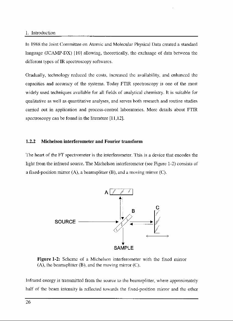
1.2.2 Michelson interferometer and Fourier transform
The heart of the FT spectrometer is the interferometer. This is a device that encodes the
light from the infrared source. The Michelson interferometer (see Figure 1-2) consists of
a fixed-position mirror (A), a beamsplitter (B), and a moving mirror (C).
AfZZ
SOURCE
SAMPLE
Figure 1-2: Scheme of a Michelson interferometer with the fixed mirror
(A), the beamsplitter (B), and the moving mirror (C).
Infrared energy is transmitted from the source to the beamsplitter, where approximately
half of the beam intensity is reflected towards the fixed-position mirror and the other
26
1.3 Diffuse reflectance
half transmitted towards the moving mirror. The returning beam from each mirror
comes back to the beamsplitter where the two beams are recombined. There they
interfere constructively or destructively, depending on the magnitude of the phase shift
between each other. This light is then directed towards the sample compartment.
From the sample, the infrared radiation reaches the detector where the remaining light is
measured and an interferogram is produced. The interferogram is a spatial-domain
{x [m]) representation of the interference patterns created in the interferometer. The
spectrum is a spatial-frequency-domain ( v ) representation of the same data. The
Fourier transform is used to decode the interferogram ( f{x) ) into a single-beam
spectrum {F{v ) ).
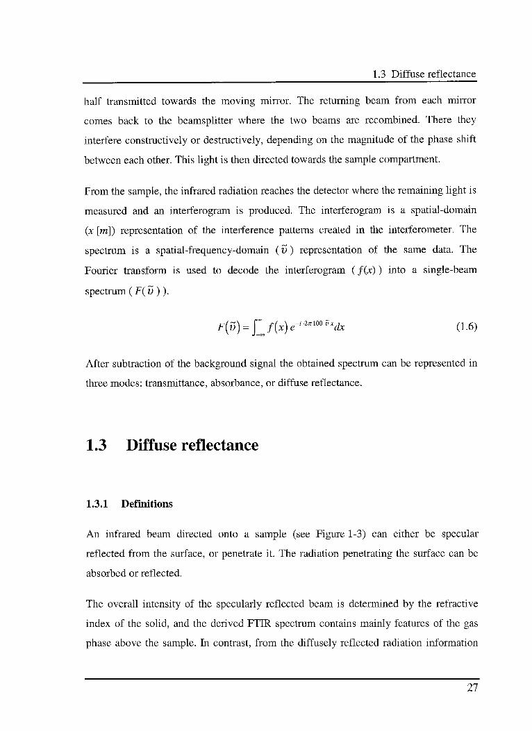
F(v) = \~j(x)e-l27im~vxdx (1.6)
After subtraction of the background signal the obtained spectrum can be represented in
three modes: transmittance, absorbance, or diffuse reflectance.
1.3 Diffuse reflectance
1.3.1 Definitions
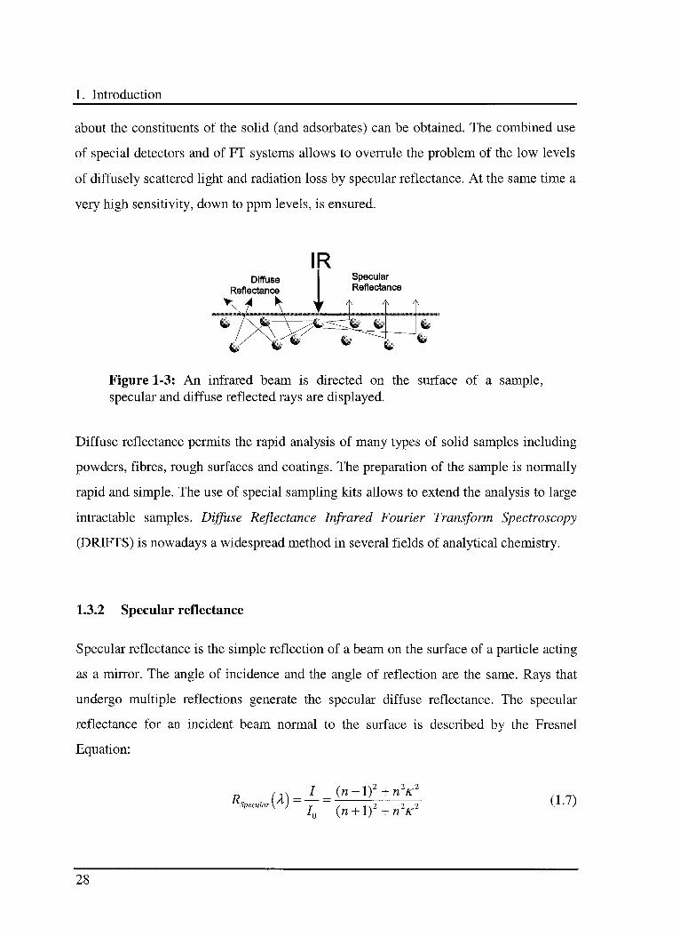
An infrared beam directed onto a sample (see Figure 1-3) can either be specular
reflected from the surface, or penetrate it. The radiation penetrating the surface can be
absorbed or reflected.
The overall intensity of the specularly reflected beam is determined by the refractive
index of the solid, and the derived FTIR spectrum contains mainly features of the gas
phase above the sample. In contrast, from the diffusely reflected radiation information
27
1. Introduction
about the constituents of the solid (and adsorbates) can be obtained. The combined use
of special detectors and of FT systems allows to overrule the problem of the low levels
of diffusely scattered light and radiation loss by specular reflectance. At the same time a
very high sensitivity, down to ppm levels, is ensured.
Diffuse
Reflectance
Figure 1-3: An infrared beam is directed on the surface of a sample,
specular and diffuse reflected rays are displayed.
Diffuse reflectance permits the rapid analysis of many types of solid samples including
powders, fibres, rough surfaces and coatings. The preparation of the sample is normally
rapid and simple. The use of special sampling kits allows to extend the analysis to large
intractable samples. Diffuse Reflectance Infrared Fourier Transform Spectroscopy
(DRIFTS) is nowadays a widespread method in several fields of analytical chemistry.
1.3.2 Specular reflectance
Specular reflectance is the simple reflection of a beam on the surface of a particle acting
as a mirror. The angle of incidence and the angle of reflection are the same. Rays that
undergo multiple reflections generate the specular diffuse reflectance. The specular
reflectance for an incident beam normal to the surface is described by the Fresnel
Equation:
RSpecular
/-\_
/ _{n-l)2 + n2K2^ '
~
I0~
{n +1)2 + n2K2(1.7)
28
1.3 Diffuse reflectance
Rspecuiar(A) is the reflectivity of an incident ray. / is the intensity of the reflected beam
and lo is the intensity of the incident beam, n is the refractive index of the sample and K
the absorption index of the matter. The absorption index is defined through Lambert's
Law:
I = I0 exp
f \7tnKl^
K j
(1.8)
where Xo denotes the wavelength of the radiation in vacuum, and I the layer thickness. It
is simple to observe that for a non-absorbing material {k~ 0) the specular reflectance
RspecuiaAA) is small except for very high values of n, whereas for strongly absorbing
substances (a:» 0) RsPecuiar(A) approaches unity, indicating a quasi total reflection of
the light beam.
1.3.3 Diffuse reflectance
Diffuse reflectance is the interaction and reflection of a beam by the surface of a
particle. The interpretation of diffuse reflectance is based on the theory developed by
Kubelka and Munk [13,14,15] and extended by Kortiim [16,17], and Kortüm et al. [18]
about the scattering of light in samples diluted in non-absorbing matrices. This model
considers that parallel layers of particles are randomly illuminated (isotropically) with
monochromatic radiation, and particles with dimensions smaller than the thickness of
the layer can absorb and/or scatter the radiation.
The obtained equation is only valid for samples of infinite thickness, i. e. samples for
which an increase in the depth does not appreciably change the spectrum. For infrared
radiation a layer of 1 - 3 mm of finely grinded powder can be considered as infinite
thickness. The diffuse reflectance R„ for a diluted sample of infinite thickness is given
by the Kubelka-Munk (K-M) Equation:
29
1. Introduction
f(Rj)=
(l R~>-2.303— (1.9)Jy '
2Rx s
where C is the concentration of the sample, a the absorptivity and s the scattering
coefficient. In practice it is not always possible to measure R„. Therefore, the relative
diffuse reflectance R/Ro is used instead, where R is the reflectance of the sample and Ro
the reflectance of the reference material.
1.3.4 Parameters affecting the DRIFT spectrum
From the theoretical point of view, it is possible to obtain spectra from samples ranging
from highly diluted to neat. In practice, the quality and the result of an analysis depend
on several parameters, the modification of which can largely affect the collected data.
Refractive index, scattering coefficient, and used diluents are the most important
parameters.
Any change of the sample refractive index [19,20,21] can significantly alter the obtained
spectrum, e. g. it may cause peak inversions, spectra which can be misinterpreted or not
even interpreted at all. Such problems can be caused by increasing coverage of adsorbed
substances [22,23]. In this case, i. e. highly concentrated samples with a high refractive
index, a dramatic increase in the specular contribution to the spectral data is observed.
To minimize this effect an adequate dilution of the sample in a non-absorbing matrix or
the use of special designed accessories [24,25,26], for a reduction of the specular
reflectance, is necessary.
Since the scattering coefficient depends on both particle size and degree of sample
packing [27,28], the linearity of the Kubelka-Munk Function can only be assured if
particle size and packing method are strictly controlled [29,30,31,32]. The particle size
is very important in diffuse reflectance measurements of powders [33,34,35,36]. Too
30
1.3 Diffuse reflectance
large particles result in the alteration of band width and intensity. Uniformly
fine-grinded samples can reduce or solve this problem.
To avoid any artefacts, the used reference or dilution matrix should not absorb radiation
at the same wavelengths as the sample. If an analytic compound is mixed with a non-
absorbing diluent it is necessary that the sample is as homogeneous as possible [37]. An
inhomogeneous distribution of the matter may affect the relative peaks intensities
[22,38].
If all of the previously discussed conditions are taken into account, quantitative accurate
measurements can be obtained [39,40,41]. Sometimes these conditions can not be
completely fulfilled. To overcome this difficulty, special ad hoc models based onto the
K-M theory have been developed [39,42,43,44,45,46,47,48].
Such models are based on reference measurements and calibration curves used to
develop the theory and the necessary mathematical equations. The validity of the models
is usually limited to the used samples and applied measurement conditions.
Modifications of these parameters frequently result in radical changes of the collected
spectra. Hence, the specialised model would no longer be valid.
1.3.5 Gas phase species in DRIFT spectroscopy
Another important feature of DRIFT spectroscopy is the possibility to observe adsorbed
as well as gas phase species at the same time. Therefore, it is possible to correlate the
gas phase composition with the observed surface compounds. Indications about gas
phase species are collected by both specular and diffusely reflected radiation. To
perform a quantitative measurement the refractive index of the sample should be nearly
constant. However, if the gas phase species react with the sample, this condition can not
always be accomplished.
31
1. Introduction
In gas phase analysis the optical path within the cell is very important, because it is
directly related to the quality of the obtained spectrum. The path inside a DRIFT cell
does usually not exceed 10 mm, which is very short compared to the ten or more meters
of a gas cell. Hence, in DRIFT cells the effects of the change of the refractive index are
enhanced by the reduced optical path. The consequences are a limited sensitivity and a
large uncertainty towards gas phase species. Therefore, quantitative measurements of
the gas phase are difficult to obtain.
1.4 DRIFT in heterogeneous catalysis
1.4.1 Introduction of DRIFT in heterogeneous catalysis
Heterogeneous catalysis is one of the numerous applications of IR spectroscopy.
Catalysis is by definition a kinetic phenomenon, yet it is noteworthy that vibrational
spectroscopy has been used to follow the transient response of kinetically significant
intermediates on heterogeneous catalysts [49,50,51,52]. One of the fundamental
approaches of vibrational spectroscopy applied to surface species is the transmission-
absorption infrared spectroscopy, which has a history dating back to 1911 [53]. This
technique offers an adequate sensitivity for weakly infrared absorbing surface species.
The main disadvantage of transmission is the necessity to press self supporting disks of
catalyst material, which must have three properties. They have to be transparent to the
IR beam, allow the throughput of the reaction gases as well as contain enough matter to
permit the observation of the surface species. Compressed catalyst disks have poor
porosity compared to the original powder. This characteristic can limit the usefulness of
transmission for in situ studies of surface reaction kinetics as a consequence of diffusion
control of reaction rates.
32
1.5 Scope of this thesis
The use of diluent powders is not a simple solution at all. The chosen material should be
completely inert towards all the components of the investigated reactions to avoid any
artefacts. The preparation of the disks is often a difficult, tedious trial and error process.
All these troubles can be partially eliminated with the use of the Diffuse Reflectance
Infrared Fourier Transform (DRIFT) spectroscopy [22,54,55,56]. This technology has
several advantages. The catalysts can be investigated in situ. The sample preparation is
unspecific and very simple, because the substance can be placed directly in the sample
holder. No dilution is normally necessary, because highly opaque, weakly absorbing and
non-reflecting materials can be analysed too. Therefore, DRIFT spectroscopy is
nowadays a very powerful tool to perform investigations in many fields of
heterogeneous catalysis.
1.4.2 Use of DRIFT in heterogeneous catalysis
DRIFT spectroscopy is, at the present, essentially applied for semiquantitative and
qualitative investigations. Quantitative measurements are usually not plausible, because
the reaction of the gas phase components with the sample induces a modification of the
refractive index of the used material. Therefore, small alterations of the reaction
conditions can induce large variations of the amount of reflected radiation. Even the
development and the application of special mathematical models, which consider these
deviations, is not simple, because a large number of parameters have to be considered
and monitored.
1.5 Scope of this thesis
Aim of the present investigation is an extension of the applicability of the FTIR/DRIFT
spectroscopy in the field of the heterogeneous catalysis. The purpose is to develop an
33

1. Introduction
analytical method, which is able to obtain qualitative and quantitative information at the
same time, i. e. reaction pathway and rate constants. The method should be insensitive
towards the used setup and the applied reaction conditions. It has to be simple, quick,
flexible, precise and economic.
34
2.1 The experimental setup
2. Experimental
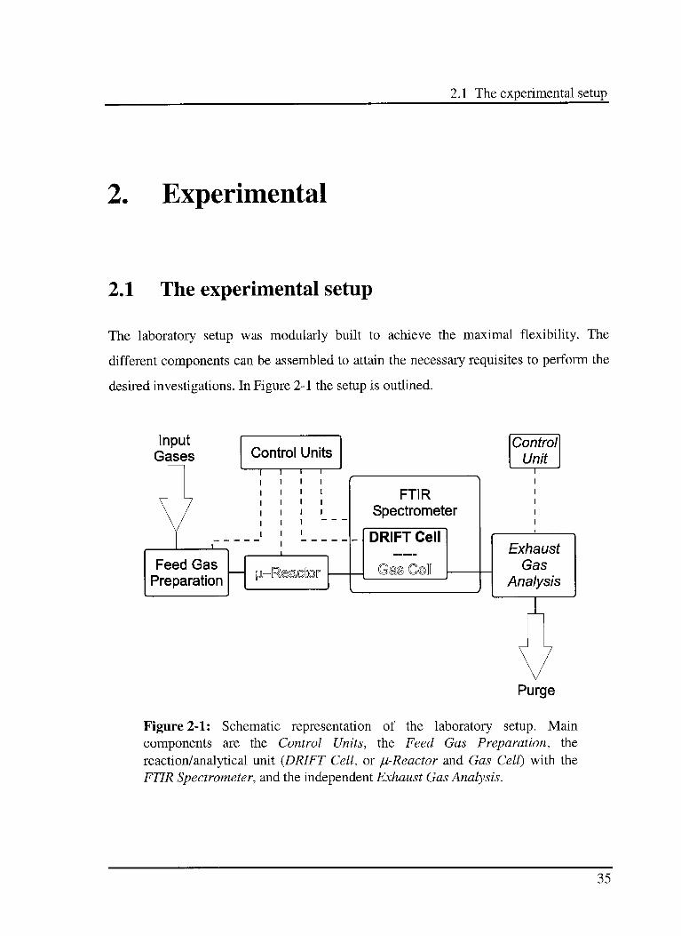
2.1 The experimental setup
The laboratory setup was modularly built to achieve the maximal flexibility. The
different components can be assembled to attain the necessary requisites to perform the
desired investigations. In Figure 2-1 the setup is outlined.
InputGases Control Units
Feed Gas
Preparation
FTIR
Spectrometer
DRIFT Cell
Control
Unit
Exhaust
Gas
Analysis
Purge
Figure 2-1: Schematic representation of the laboratory setup. Main
components are the Control Units, the Feed Gas Preparation, the
reaction/analytical unit {DRIFT Cell, or ju-Reactor and Gas Cell) with the
FTIR Spectrometer, and the independent Exhaust Gas Analysis.
35
2. Experimental
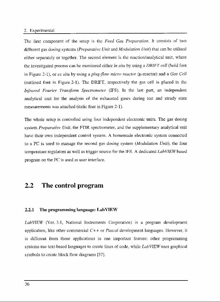
The first component of the setup is the Feed Gas Preparation. It consists of two
different gas dosing systems {Preparative Unit and Modulation Unit) that can be utilised
either separately or together. The second element is the reaction/analytical unit, where
the investigated process can be monitored either in situ by using a DRIFT cell (bold font
in Figure 2-1), or ex situ by using a plug-flow micro reactor ((i-reactor) and a Gas Cell
(outlined font in Figure 2-1). The DRIFT, respectively the gas cell is placed in the
Infrared Fourier Transform Spectrometer (IFS). In the last part, an independent
analytical unit for the analysis of the exhausted gases during test and steady state
measurements was attached (italic font in Figure 2-1).
The whole setup is controlled using four independent electronic units. The gas dosing
system Preparative Unit, the FTIR spectrometer, and the supplementary analytical unit
have their own independent control system. A homemade electronic system connected
to a PC is used to manage the second gas dosing system {Modulation Unit), the four
temperature regulators as well as trigger source for the IFS. A dedicated LabVIEWbased
program on the PC is used as user interface.
2.2 The control program
2.2.1 The programming language: LabVIEW
LabVIEW (Ver. 3.1, National Instruments Corporation) is a program development
application, like other commercial C++ or Pascal development languages. However, it
is different from those applications in one important feature: other programming
systems use text-based languages to create lines of code, while LabVIEW uses graphical
symbols to create block flow diagrams [57].
36
2.2 The control program
LabVIEW uses the concept of modular programming. An application is divided into a
series of dedicated tasks, which can be further divided until a complicated application
becomes a series of simple subtasks. The final recombination of all subtasks represents
the program.
2.2.2 The control program
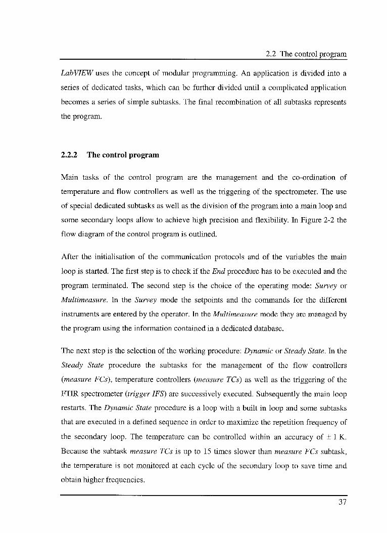
Main tasks of the control program are the management and the co-ordination of
temperature and flow controllers as well as the triggering of the spectrometer. The use
of special dedicated subtasks as well as the division of the program into a main loop and
some secondary loops allow to achieve high precision and flexibility. In Figure 2-2 the
flow diagram of the control program is outlined.
After the initialisation of the communication protocols and of the variables the main
loop is started. The first step is to check if the End procedure has to be executed and the
program terminated. The second step is the choice of the operating mode: Survey or
Multimeasure. In the Survey mode the setpoints and the commands for the different
instruments are entered by the operator. In the Multimeasure mode they are managed by
the program using the information contained in a dedicated database.
The next step is the selection of the working procedure: Dynamic or Steady State. In the
Steady State procedure the subtasks for the management of the flow controllers
{measure FCs), temperature controllers {measure TCs) as well as the triggering of the
FTIR spectrometer {trigger IFS) are successively executed. Subsequently the main loop
restarts. The Dynamic State procedure is a loop with a built in loop and some subtasks
that are executed in a defined sequence in order to maximize the repetition frequency of
the secondary loop. The temperature can be controlled within an accuracy of ± 1 K.
Because the subtask measure TCs is up to 15 times slower than measure FCs subtask,
the temperature is not monitored at each cycle of the secondary loop to save time and
obtain higher frequencies.
37
2. Experimental
database
Multi-
measure
measure
FCs
measure
TCs
For Each
Cycleu
triggerIFS
measure
TCs
i-Q
N
measure
FCs
Unti All
Cycles
Next Cycle
Figure 2-2: Flow diagram of the control program. Main components are the
main loop, with the Steady State and the Dynamic State loops, as well as the
subtasks measure FCs, measure TCs and trigger IFS.
38
2.2 The control program
The Dynamic State loop checks first if the routine to send the trigger signal to the FTIR
spectrometer {trigger IFS) has to be executed. The secondary loop is then started and
repeated for a specified number of accumulations. Each cycle start checking if the
temperatures have to be measured, and if so, the routine measure TCs is then executed.
Then the subtask measure FCs is executed and the cycle ends. When the secondary loop
is terminated the Dynamic State loop ends too. The program can then either restart
another Dynamic State loop or the main loop. To avoid possible conflicts between
commands simple Errors-Controls are implemented [58].
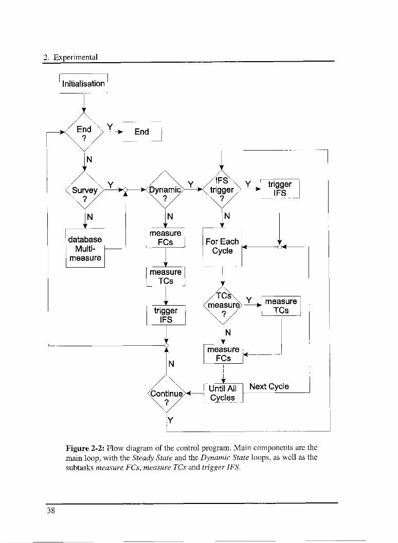
2.2.3 Management of the mass flow controllers {measure FCs)
The four mass flow controllers and the liquid flow controller (FCs) of the Modulation
Unit have to be managed with high precision and flexibility. The programmed subtask
has to adjust the setpoints and to monitor the output.
/\New\
xValues/Y Data
Base
>
N
i ^ '
Read
Values
Set
Values
Figure 2-3: Flow diagram of the subtask dedicated for the management of
theflow controllers (FCs). Further details are given in the text.
39
2. Experimental
The programmed subtask has to adjust the setpoints and monitor the output. The flows
have to be changed either sinusoidally or stepwise, and the total flow has to stay
constant. The regulation of a single FC for the use of fluids which differ from the
calibration fluid has to be simple. A quick data transmission is essentially to minimize
the reaction time and to maximize the frequency of the applied sinusoidal patterns. The
flow diagram of the subtask is shown in Figure 2-3.
The communication between PC and FCs occurs via two high-performance acquisition
boards, AT-A0-6 and AT-MIO-16XE-50 (both National Instruments), for analogue
output and digital input/output. Two connector blocks, CB-50 and SCB-68 (both
National Instruments), are used as physical interfaces between the control PC and the
electronic unit. The advantage of the use of this setup is the parallel control of all FCs.
To speed up the execution of the subtask a simple method, based on the multiplication
of two matrices, was applied. In this way the whole subtask can be accomplished in a
single run, and iteration frequencies up to 90 Hz are reached. The database-matrix
carries the correction parameters to convert setpoints and output values from calibration
fluids to applied fluids and vice versa [59,60]. The values-matrix is used to store
setpoints and output values. The first step of the sub task looks for new setpoints and
conversion values. Old parameters of the two matrices are replaced by the new data. The
new setpoints are converted using the database-matrix, and sent to the FCs. If no
changes are necessary this step is skipped. The output values are collected, transformed
using the database-matrix, and the results are stored in the values-matrix. Then the
subtask ends.
The control of the total flow is obtained by using a flow controller to compensate any
variations of the volume caused by variation of the reactive components. Each fluid
flow is adjusted using a polynomial 3rd degree calibration function [59,60,61]. The
achieved maximal deviation is ± 0.3 %.
40
2.2 The control program
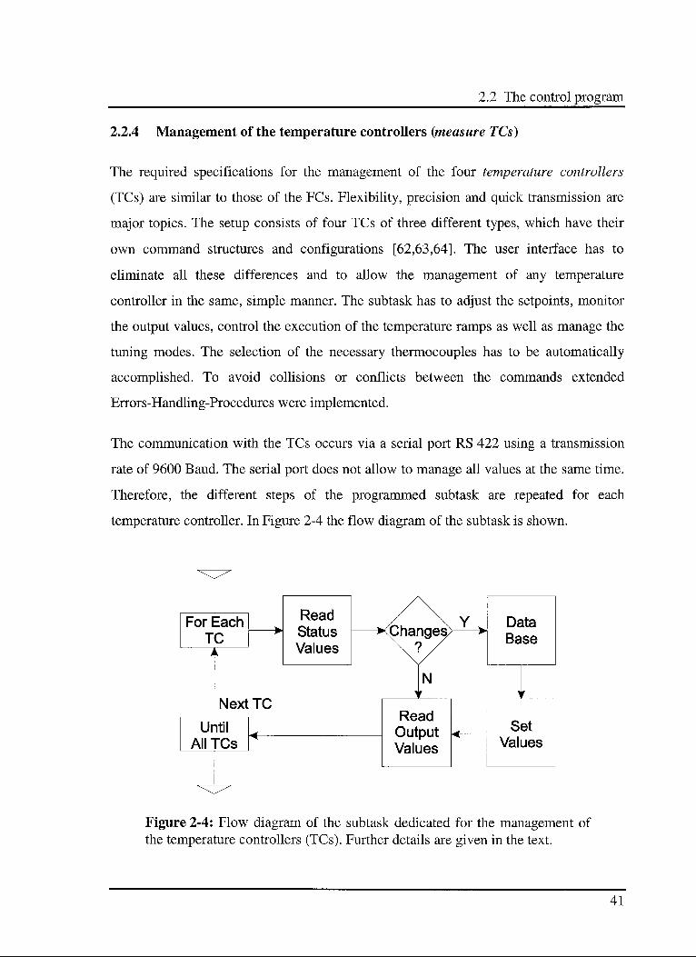
2.2.4 Management of the temperature controllers {measure TCs)
The required specifications for the management of the four temperature controllers
(TCs) are similar to those of the FCs. Flexibility, precision and quick transmission are
major topics. The setup consists of four TCs of three different types, which have their
own command structures and configurations [62,63,64]. The user interface has to
eliminate all these differences and to allow the management of any temperature
controller in the same, simple manner. The subtask has to adjust the setpoints, monitor
the output values, control the execution of the temperature ramps as well as manage the
tuning modes. The selection of the necessary thermocouples has to be automatically
accomplished. To avoid collisions or conflicts between the commands extended
Errors-Handling-Procedures were implemented.
The communication with the TCs occurs via a serial port RS 422 using a transmission
rate of 9600 Baud. The serial port does not allow to manage all values at the same time.
Therefore, the different steps of the programmed subtask are repeated for each
temperature controller. In Figure 2-4 the flow diagram of the subtask is shown.
Read
Status
Values
Data
Base
For Each
TC<Changea>\ o /
Y.
w
> k \. " /
^
Nr > '
Next ICRead
OutputValues
<Set
Values
Until
All"res
Figure 2-4: Flow diagram of the subtask dedicated for the management of
the temperature controllers (TCs). Further details are given in the text.
41
2. Experimental
In this case a programming technique based on two matrices is also used. A
database-matrix contains setting values and status flags. A values-matrix is used for the
setpoints and output values. In the first step the program collects information about the
actual status of the TC. In the second, the occurred changes and the new values are
combined and elaborated, the database-matrix is updated, the new setpoints converted
and the necessary commands are sent to the TC. The steps are skipped if no changes are
indicated. In the last step the output values are collected, using the database-matrix,
converted and stored in the values-matrix. Then the whole task is repeated for another
TC. As in the FCs subtask only the necessary operations are performed.
The selection of the thermocouple is obtained by sending the necessary command
sequences and putting the TC off-line for several seconds. Temperature ramp programs
and tune modes of the TCs are activated by starting the dedicated request procedures.
The use of self and adaptive tune programs results in a maximum temperature deviation
of ± 1 K. The achieved mean iteration time is 175 ms for each TC.
2.2.5 The triggering of the spectrometer {trigger IFS)
The triggering of the FTIR spectrometer (see section 2.6) is used to set the starting
points for time resolved measurements. Therefore, the management of the data
communications with the FTIR spectrometer is very important. A simple data protocol
is essential to permit a fast transmission and therefore a minimal time delay between
send of the start signal {-trigger now-) and start of the measurement. The subtask trigger
IFS has to monitor the actual status of the IFS and of the running measurement but also
to coordinate the start of new measurements by setting the trigger flag.
A high-performance acquisition board AT-MIO-16XE-50 for analogue output and digital
input/output and a connector block CB-50 (both National Instruments) are used as
communication interface between the control PC and IFS. The advantage of this setup is
42
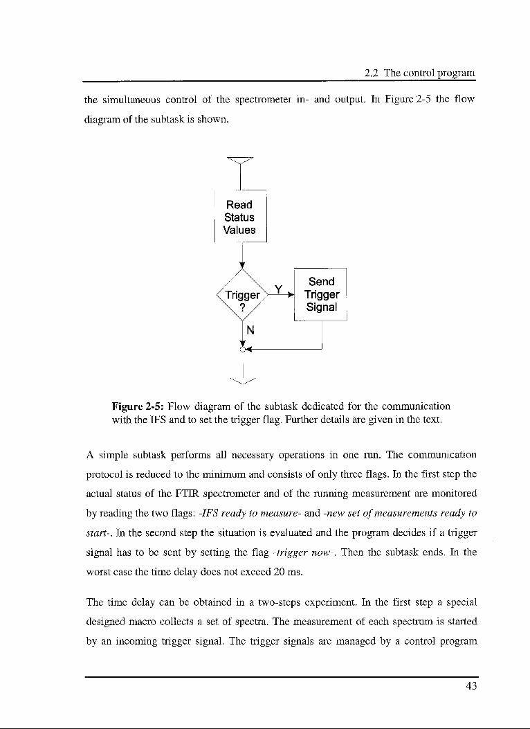
2.2 The control program
the simultaneous control of the spectrometer in- and output. In Figure 2-5 the flow
diagram of the subtask is shown.
Figure 2-5: Flow diagram of the subtask dedicated for the communication
with the IFS and to set the trigger flag. Further details are given in the text.
A simple subtask performs all necessary operations in one run. The communication
protocol is reduced to the minimum and consists of only three flags. In the first step the
actual status of the FTIR spectrometer and of the running measurement are monitored
by reading the two flags: -IFS ready to measure- and -new set ofmeasurements ready to
start-. In the second step the situation is evaluated and the program decides if a trigger
signal has to be sent by setting the flag -trigger now-. Then the subtask ends. In the
worst case the time delay does not exceed 20 ms.
The time delay can be obtained in a two-steps experiment. In the first step a special
designed macro collects a set of spectra. The measurement of each spectrum is started
by an incoming trigger signal. The trigger signals are managed by a control program
43
2. Experimental
which can send an impulse every 10 ms. The time at which the spectrum is collected is
automatically stored by the FTIR spectrometer. The first starting time is subtracted from
the last one, then this value is divided by the number of collected spectra. The mean
time necessary for the collection of a spectrum - wait for trigger signal - interpretation
of the signal - start next measurement is obtained.
In a second step a macro collects a set of spectra without waiting for trigger signals.
Identical to the first step the mean value between starting times is calculated. In this case
the mean time for collection ofa spectrum - start the next measurement is obtained. The
difference between the first and the second mean time is the value for wait for trigger
signal - interpretation of the signal. This interval corresponds to the time delay between
the start signal {-trigger now-) and start of the measurement.
2.3 The gas dosing systems
2.3.1 The Preparative Unit
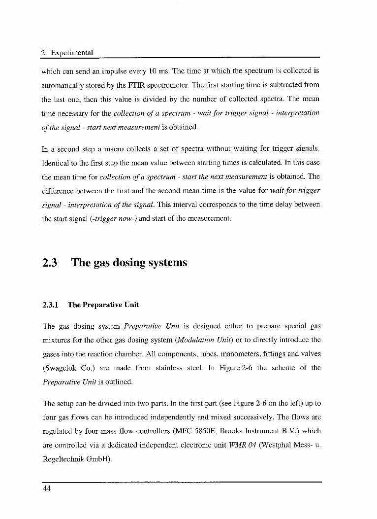
The gas dosing system Preparative Unit is designed either to prepare special gas
mixtures for the other gas dosing system {Modulation Unit) or to directly introduce the
gases into the reaction chamber. All components, tubes, manometers, fittings and valves
(Swagelok Co.) are made from stainless steel. In Figure 2-6 the scheme of the
Preparative Unit is outlined.
The setup can be divided into two parts. In the first part (see Figure 2-6 on the left) up to
four gas flows can be introduced independently and mixed successively. The flows are
regulated by four mass flow controllers (MFC 5850E, Brooks Instrument B.V.) which
are controlled via a dedicated independent electronic unit WMR 04 (Westphal Mess- u.
Regeltechnik GmbH).
44
2.3 The gas dosing systems
WMR04
GAS1 cr£>-
GAS2 cz[>-
GAS3c4>-
-£°a
-CxO
GAS4i^>-
-IX}
-ix}
TO THE
W-<> REACTOR
ANALYSIS
FROM THE
REACTOR
JL
PURGE
Figure 2-6: Schematic representation of the Preparative Unit. Main partsare the preparation (left) and the pressure regulation (bottom right).
In the second part (see Figure 2-6 bottom right) a manometer, ON/OFF valves and
needle valves with different Flow Coefficient (Cy) are used to regulate the desired
pressure within the reaction chamber.
The three lines are parallel mounted. In the middle line a needle valve with a small Cy
(0.004) is used to control the gas flow down to 10 mlN min"1. The lower line consists of
a needle valve with a higher Cy (0.03) and an ON/OFF valve. This is used to control the
pressure at higher gas flows. The upper line is equipped with an ON/OFF valve. In this
way it is possible to bypass the two other lines without changing the settings of the
needle valves. This is useful for flushing samples prior, during or after other
experiments. This special designed setup is very sensitive to pressure control. The
desired pressure value is quickly reached, and is held without detectable changes over a
long period. Two exits are used to connect additional analytical units.
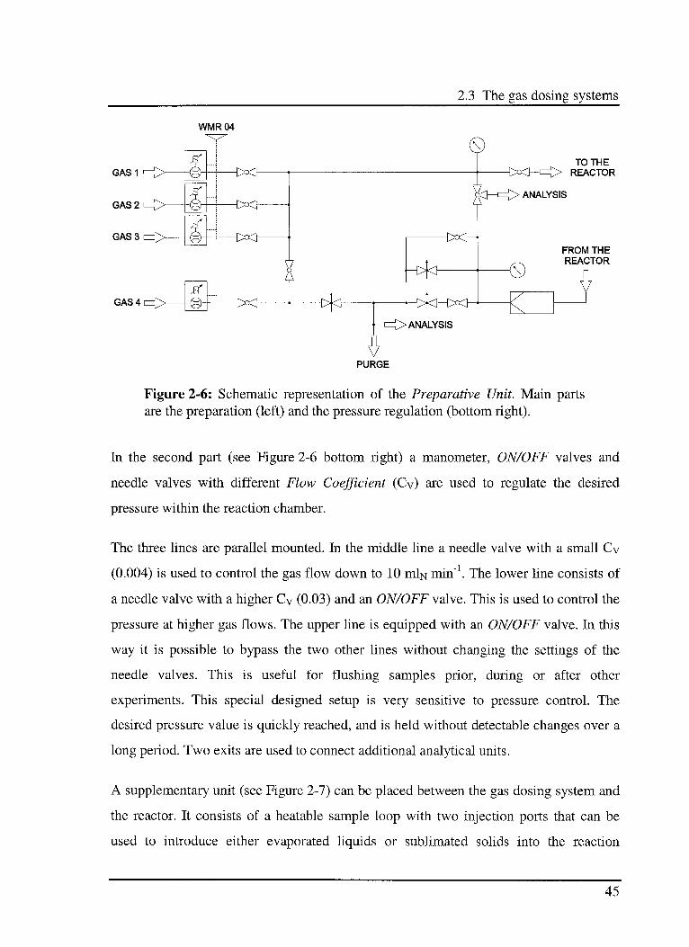
A supplementary unit (see Figure 2-7) can be placed between the gas dosing system and
the reactor. It consists of a heatable sample loop with two injection ports that can be
used to introduce either evaporated liquids or sublimated solids into the reaction
45
2. Experimental
chamber. This unit consists of two parallel lines. When a substance is introduced in one
loop, the gas flow is directed to the other line.
CONTROL UNITv
LIQUID^^ {TJ
FROM THE
GAS-DOSING
SYSTEM
Figure 2-7: Schematic view of the supplementary unit of the PreparativeUnit. Main components are the heatable sample loop and the two injection
ports.
Then the gas flow is switched to the line containing the evaporated or sublimated
compound. The loop can be heated up to 473 K using a heating tape (Hillesheim
GmbH), while the temperature is controlled by a digital temperature regulator (model
94C, Eurotherm Regler GmbH). The thermocouple (Type K, 0 1 mm) is placed at the
gas exit.
2.3.2 The Modulation Unit
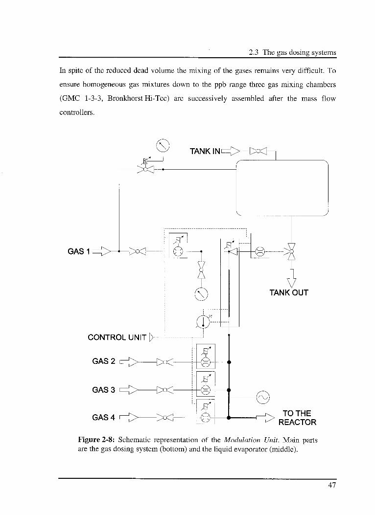
The second gas dosing system Modulation Unit is designed to independently introduce
up to four gases and one liquid into the reaction chamber. All components, tubes,
manometers, fittings and valves (Swagelok Co.) are made from stainless steel. The
diameter of the tubes was chosen in order to obtain a minimal dead volume. The gas
flows are regulated to the desired values using mass flow controllers (MFC
F-201C-FA-31, Bronkhorst Hi-Tec).
46
SOLID
TO THE
REACTOR
2.3 The gas dosing systems
In spite of the reduced dead volume the mixing of the gases remains very difficult. To
ensure homogeneous gas mixtures down to the ppb range three gas mixing chambers
(GMC 1-3-3, Bronkhorst Hi-Tec) are successively assembled after the mass flow
controllers.
GAS1
CONTROL UNIT
GAS 2
GAS 3
GAS 4TO THE
REACTOR
Figure 2-8: Schematic representation of the Modulation Unit. Main partsare the gas dosing system (bottom) and the liquid evaporator (middle).
47
2. Experimental
To avoid possible condensation in the system the mixing chambers are heated by a
semiconductor-based heating tape HBRT40 (Hillesheim GmbH) allowing a maximum
temperature of 393 K.
The liquid is placed in a 0.2 1 high pressure stainless steel tank, its flow is monitored via
a liquid flow controller (LF Ll-FA-11-0, Bronkhorst Hi-Tec) and regulated by an
electromagnetic needle valve at the top of the evaporation unit. Then the liquid is
introduced into the controlled evaporator mixer (CEM W-102-131-P,
Bronkhorst Hi-Tec).
A digital temperature regulator (model 94C Eurotherm Regler GmbH) is used to control
the temperature in the evaporation unit. The thermocouple (Type PtlOO) is placed at the
gas exit. The mass flow controllers, the liquid flow controller and the temperature
controller are managed through a dedicated homemade electronic system connected to
the control PC using the LabVIEW based program.
2.4 DRIFT: optical accessories and methodic
Two different environmental chambers are used, which allow to emulate process
conditions.
2.4.1 Controlled Environmental Chamber
The Controlled Environmental Chamber (Model 0030-102, Spectra-Tech) is suitable for
experiments requiring temperatures up to 1173 K and pressures among 104 Pa and
0.7 MPa. The chamber hood is fitted with two NaCl windows (transparent from 48TOO
to 650 cm4) (Korth Kristalle GmbH).
48
2.4 DRIFT: optical accessories and methodic
The sample holder has a volume of about 0.1 ml, and the reaction gases flow over the
sample. The heater element is part of the sample holder. The thermocouple (Type K,
0 0.5 mm) is placed directly below the sample holder surface. The temperature is
controlled using a digital temperature regulator (model 94C Eurotherm Regler GmbH).
A water cooling canal is contained, below the steel dome, in the top part of the cell
support, to protect the gaskets from high temperatures. A gas-tight attachment of the
steel dome over the cell support is obtained by viton O-rings. A schematic view of the
DRIFT cell can be found elsewhere [65].
The environmental chamber is placed in the COLLECTOR (Diffuse Reflectance
Accessory 0030-0XX, Spectra-Tech). Its characteristic is the measurement in on-axis
geometry that provides a high energy throughput. Some modifications of the original
design were carried out in order to obtain a quick and better fixation of the whole unit in
the measurement chamber of the FTIR spectrometer. Further details about the accessory
can be found elsewhere [66].
Test measurements have shown that, under the applied conditions, the specular
reflectance effect is normally very weak or not present at all. No pronounced artefacts
could be detected.
2.4.2 Environmental Chamber
The Environmental Chamber (HT-HP EC 19933, Graseby-Specac) is suitable for
experiments requiring temperatures up to 773 K and pressures between 10"4 Pa and
3.3 MPa. The chamber hood is fitted with a ZnSe window (transparent from 20'000 to
455 cm"1).
A volume of about 0.1 ml of material can be loaded into the sample holder. The original
design was modified in order to allow the reaction gases to pass through the sample. A
mesh, placed at the bottom of the sample holder where the gases enter, acts as support
49
2. Experimental
for the loaded compound and distributes the gas flow uniformly through the whole
sample. The heater element is part of the sample holder. The thermocouple (Type PtlOO,
0 1.0 mm) is placed directly below the sample holder surface. The temperature is
controlled using a digital temperature regulator (model 847, Eurotherm Regler GmbH).
A water-cooling body is placed between the cell support and the dome, to protect the
gaskets from the high temperatures. A gas-tight attachment of the steel dome over the
cell support is obtained by viton O-rings. A schematic view of the DRIFT cell can be
found elsewhere [67].
Test measurements, using two thermocouples (Type K, 0 0.33 mm, Philips A.G.),
placed on the surface and the bottom of the catalyst bed in the sample holder, have
shown that the thermal gradient is below 1.5 K ± 0.5 K.
The environmental chamber was placed in the SELECTOR (Diffuse Reflectance
Accessory 19900, Graseby-Specac). The measurements in off-axis geometry ensure the
minimization of unwanted specular reflectance. A scheme of this accessory can be
found elsewhere [68].
2.4.3 Representation of DRIFT spectra
The DRIFT spectra are usually displayed in Kubelka-Munk units. Catalysts of
greyish-black colour absorb strongly throughout the MIR region, and their reflectance
during the reaction {R) is higher than those of freshly pretreated catalysts which are used
as reference {Ro). These properties violate one of the basic assumptions of the Kubelka-
Munk theory, i. e. the presence of a non- or weakly absorbing substrate [13,14,15].
Therefore, in this work the spectra will be presented as relative reflectance units {R/Ro).
Several authors use multiplication of the background spectrum by a factor of 20 [69] in
the K-M equation or the logarithm of the inverse of the reflectance [70,71] instead of the
50
2.5 The micro reactor / gas cell system
K-M model. However, these procedures are not suitable when desorption or reactive
consumption of surface species must be considered. Therefore, the use of relative
reflectance units, which are directly related to the experiment, is more appropriate.
The dilution of the sample with a non-absorbing substance is not possible in
heterogeneous catalysis. Alkali halides (KCl, KBr, ...) are chemically not inert under the
applied conditions and react either with the catalyst or with the reaction gases. Other
diluents (e. g. metal oxides, ...) can perturb the reaction via secondary reactions or
induce the migration of adsorbed species, i. e. spillover, between the different sample
components.
2.4.4 Sample preparation
As mentioned in the previous chapter, DRIFT spectra are greatly influenced by sample
packing [29,30,31]. The duration and the pressure applied to the sample are critical in
affecting the scattering coefficients. To ensure the reproducibility of the experiments,
the catalyst is pressed, for 0.5 to 1 minute, with a constant pressure of 1 MPa into the
sample holder of the environmental chamber with a home made sample packing device
[72]. Test experiments performed with this packing system have shown reproducibility
of the spectra with a small standard deviation [73].
2.5 The micro reactor / gas cell system
The setup consists of a plug flow micro reactor (|J,-reactor) placed in a vertically
mounted furnace and a gas cell. This system is suitable for experiments requiring
temperatures up to 973 K and pressures among 0.1 and 4 MPa. A scheme of the setup is
outlined in Figure 2-9.
51
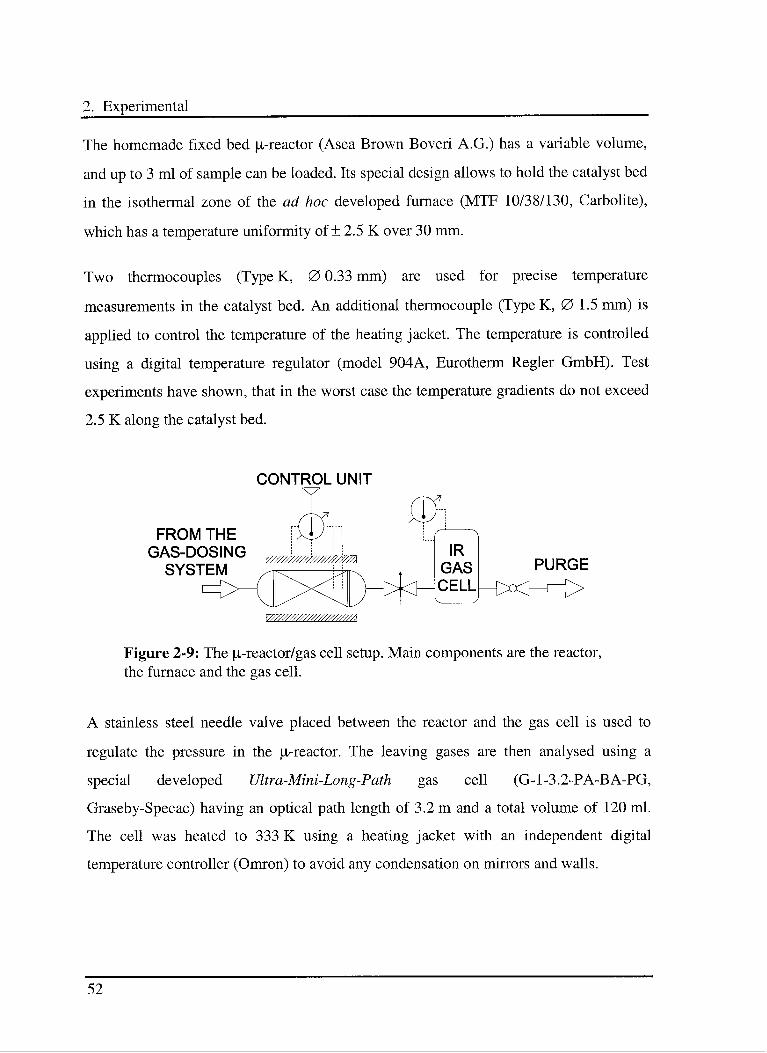
2. Experimental
The homemade fixed bed ji-reactor (Asea Brown Boveri A.G.) has a variable volume,
and up to 3 ml of sample can be loaded. Its special design allows to hold the catalyst bed
in the isothermal zone of the ad hoc developed furnace (MTF 10/38/130, Carbolite),
which has a temperature uniformity of ± 2.5 K over 30 mm.
Two thermocouples (Type K, 0 0.33 mm) are used for precise temperature
measurements in the catalyst bed. An additional thermocouple (TypeK, 0 1.5 mm) is
applied to control the temperature of the heating jacket. The temperature is controlled
using a digital temperature regulator (model 904A, Eurotherm Regler GmbH). Test
experiments have shown, that in the worst case the temperature gradients do not exceed
2.5 K along the catalyst bed.
CONTROL UNIT
FROM THE
GAS-DOSING
SYSTEMY////////////////////7//A
IR
GAS
CELL
PURGE
Y///////////////////////A
Figure 2-9: The u.-reactor/gas cell setup. Main components are the reactor,
the furnace and the gas cell.
A stainless steel needle valve placed between the reactor and the gas cell is used to
regulate the pressure in the |J,-reactor. The leaving gases are then analysed using a
special developed Ultra-Mini-Long-Path gas cell (G-1-3.2-PA-BA-PG,
Graseby-Specac) having an optical path length of 3.2 m and a total volume of 120 ml.
The cell was heated to 333 K using a heating jacket with an independent digital
temperature controller (Omron) to avoid any condensation on mirrors and walls.
52
2.6 The FTIR spectrometer
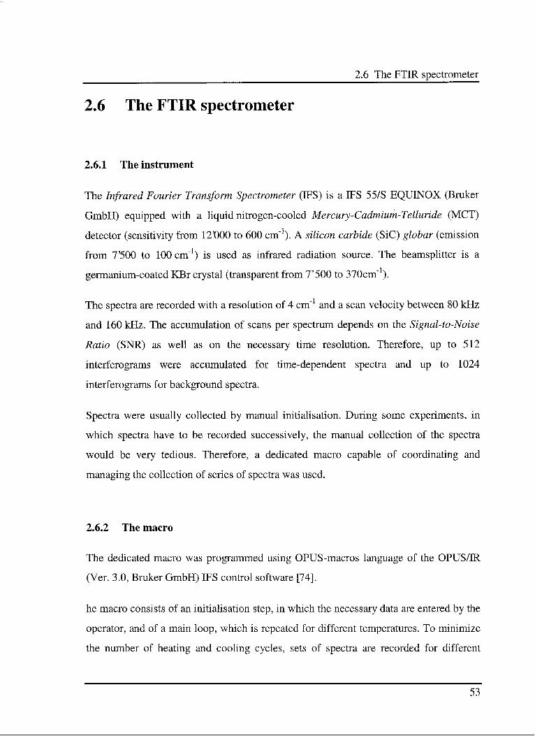
2.6 The FTIR spectrometer
2.6.1 The instrument
The Infrared Fourier Transform Spectrometer (IFS) is a IFS 55/S EQUINOX (Bruker
GmbH) equipped with a liquid nitrogen-cooled Mercury-Cadmium-Telluride (MCT)
detector (sensitivity from 12X)00 to 600 cm"1). A silicon carbide (SiC) globar (emission
from 7'500 to 100 cm"1) is used as infrared radiation source. The beamsplitter is a
germanium-coated KBr crystal (transparent from 7'500 to 370cm"1).
The spectra are recorded with a resolution of 4 cm"1 and a scan velocity between 80 kHz
and 160 kHz. The accumulation of scans per spectrum depends on the Signal-to-Noise
Ratio (SNR) as well as on the necessary time resolution. Therefore, up to 512
interferograms were accumulated for time-dependent spectra and up to 1024
interferograms for background spectra.
Spectra were usually collected by manual initialisation. During some experiments, in
which spectra have to be recorded successively, the manual collection of the spectra
would be very tedious. Therefore, a dedicated macro capable of coordinating and
managing the collection of series of spectra was used.
2.6.2 The macro
The dedicated macro was programmed using OPUS-macros language of the OPUS/IR
(Ver. 3.0, Bruker GmbH) IFS control software [74].
he macro consists of an initialisation step, in which the necessary data are entered by the
operator, and of a main loop, which is repeated for different temperatures. To minimize
the number of heating and cooling cycles, sets of spectra are recorded for different
53
2. Experimental
parameters at a chosen temperature. Then the same sequence is repeated at a new
temperature.
Initialisation
IFor Each
TemperatureSet Status —>
Reference
Spectrat k
v
Until All
Temperatures< Set Status <
Measurement
Spectra
> '
End
Figure 2-10: Flow diagram of the macro used to perform multiplemeasurements during experiments. Further details are given in the text.
The first step of the loop is the setting of flags. Two flags -IFS ready to measure- and
-new set of measurements ready to start- are used to indicate the status of the IFS and
the measurement. The first flag indicates when new spectra can be collected. The second
flag is used to control the start of a new set of measurements at a new temperature. Two
similar submacros are started subsequently: one for the accumulation of reference
spectra, the other for the collection of measurement spectra. The flags are then reset and
the loop can be restarted for a new temperature.
Both submacros have the same flow diagram, but differ for the number of collected
interferograms per sample and background spectra. The task of these submacros is to
coordinate the collection of spectra. In Figure 2-11 the flow diagram of the submacros is
shown.
54
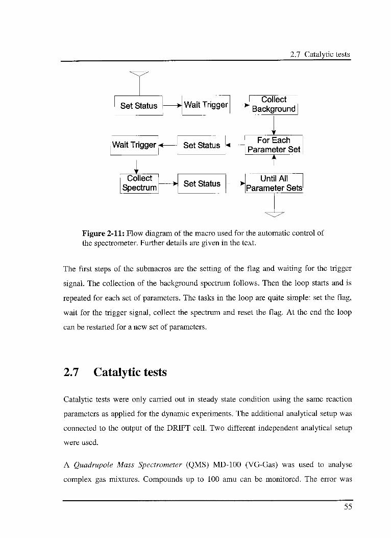
2.7 Catalytic tests
Set Status Wait TriggerCollect
Background
Wait Trigger <— Set Status <For Each
Parameter Set
^ ' ÎCollect
Spectrum— Set Status
Until All
Parameter Sets
Figure 2-11: Flow diagram of the macro used for the automatic control of
the spectrometer. Further details are given in the text.
The first steps of the submacros are the setting of the flag and waiting for the trigger
signal. The collection of the background spectrum follows. Then the loop starts and is
repeated for each set of parameters. The tasks in the loop are quite simple: set the flag,
wait for the trigger signal, collect the spectrum and reset the flag. At the end the loop
can be restarted for a new set of parameters.
2.7 Catalytic tests
Catalytic tests were only carried out in steady state condition using the same reaction
parameters as applied for the dynamic experiments. The additional analytical setup was
connected to the output of the DRIFT cell. Two different independent analytical setup
were used.
A Quadrupole Mass Spectrometer (QMS) MD-100 (VG-Gas) was used to analyse
complex gas mixtures. Compounds up to 100 amu can be monitored. The error was
55
2. Experimental
estimated to be ± 2 % of the measured value. A Siemens IR CO/CO2 analyser was used
to measure carbon monoxide and carbon dioxide. The error of the apparatus was ± 5 %
of the measured value.
2.8 Compounds
Nitrogen, that was used as carrier gas, as well as carbon monoxide, carbon dioxide,
hydrogen and oxygen were used without further purification. All gases were
commercially available (Sauerstoff Lenzburg A.G.) in 5.0 quality (purity >99.999 %).
Formic acid, methanol and paraformaldehyde (both Fluka purum > 98%) were used as
1 T
reference substances; labelled formic acid and paraformaldehyde (both > 99%, C;
chemical purity > 98%) were obtained from Cambridge Isotope Laboratories.
The Pd25Zr75 catalyst for the CO oxidation was prepared by the melt spinning technique
[75]. The Cu4öZr54 catalyst for the C02/CO hydrogénation to methanol was prepared by
coprecipitation of the corresponding metal nitrates, at constant pH and temperature, as
described elsewhere [76,77]. Both catalysts were prepared in the group of Prof. Dr. A.
Baiker at the Swiss Federal Institute of Technology, ETH Zürich, Switzerland. We
thank him for making available these samples.
The Cu/Zn0/Al203 catalyst for the CO/CO2 hydrogénation to methanol was provided by
Haldor Tops0e A/S.
56
3.1 Introduction
3. Reactants modulation
3.1 Introduction
The characterisation of catalytic reactions is important for the production of new
catalysts, and for the optimisation of industrial catalytic processes [78,79,80]. The
primary goal of the characterisation is to provide a basis for understanding the activity
and selectivity of the investigated system. The secondary goal is to obtain all necessary
information in order to develop better catalysts and find the best working conditions.
From a systems theory point of view, investigated catalytic processes can be considered
as unknown systems with their own internal rules. The investigation of unknown
systems and the determination of the governing rules is one of the main tasks of the
Control System Theory [81,82,83] and of the Signal Processing Theory [84,85,86]. The
investigation is based on the application of theoretical concepts to the experimental
result.
In the theoretical analysis existing information is used to create complete models and to
evaluate possible modifications allowing high flexibility. The developed model can be
rapidly and simplyadaptedtodescribesimilarsystems.Thedisadvantageistheimpossibilitytoknowaprioriiftheobtainedmodelwillbeappropriate.Theexperimentalanalysisusesexperimentallyobtaineddatatodevelopamodel.Asimplemodelisnormallyenoughtodescribetherawdata,butnonewknowledgeabouttheinvestigatedsystemcanbeacquired.Bestresultsareobtainedbymodifyingatheoreticalmodeltomatchtheexperimentaldata.
57
3. Reactants modulation
A similar procedure is used in the modulation analytical concept in heterogeneous
catalysis, to be described below, in order to obtain information about reaction pathways
and reaction rate constants of a catalytic system. In this new concept theoretical
knowledge is used to create models, which are modified to match the experimental data.
Models that adequately represent the reality are obtained using the classical method of
fitting the experimental data to the control system models.
An external perturbation applied to the system induces time-dependent selective
modifications of the different components. The temporal evolution of the signals is
monitored over large spectral intervals. Then the collected data are elaborated and fitted
to the applied model. Information about the processes occurring in the system are thus
obtained.
In the 2D correlation techniques, extensively applied in NMR [87,88,89,90] and IR
[91,92,93,94,95] spectroscopy, two different perturbations were used to obtain
additional information about the investigated system.
In the field of heterogeneous catalysis several methods based on a similar idea were
used, e. g. Transient Response Methods, Temperature Programmed Desorption and
Temperature Programmed Reaction [96,97,98]. Theoretical studies of the application of
Frequency Response techniques to catalytic systems were presented by several authors
[99,100,101,102]. More recently, practical applications of these techniques were used in
the investigation of adsorption kinetics of gases [103,104] and catalytic systems
[105,106,107].
58
3.2 Approach to the problem
3.2 Approach to the problem
In our approach the equilibrium of a system is perturbed by a test signal. The choice of
this test signal is very important, because it influences directly the output signals. These
have to be monitored and should not be influenced by the setup.
For heterogeneously catalysed reactions studied by DRIFT spectroscopy, the choice of
the test signal is not very simple. As explained in the first chapter, small variations of
the sample refractive index induce large changes in the measured values. Therefore, test
signals, e. g. ramps or step up/step down, where information about the system are
obtained from the form and intensity of the output signals, are not often applicable.
The problem of the refractive index can be solved by using repetitive test signals, e. g.
sinusoidal waves. In such a case the system influences form, intensity and position of
the output signals. The output signal is also sinusoidal, and maxima respectively minima
in the concentrations unambiguously correspond to maxima and minima in the
measured values. Information about the investigated system can hence be obtained from
the position, or phase lag, of the output signals.
In gas phase FTIR spectroscopy, the use of sinusoidal functions as test signals allows
the elimination of calibration curves.
Heterogeneous catalytic systems can be perturbed by varying different parameters, i. e.
temperature, total pressure and reactant concentrations in the feed gas. Modulation of
the temperature induces the parallel modification of all reaction components. In this
case it is very difficult to observe selective changes of single components. Due to the
superposition of the system answers, the information can not be easily extracted.
Modulation of the total pressure or of a single component, participating in different
steps of the process, allows the reduction of the responses superposition, and therefore
conclusions can be drawn. On the other hand, the modulation of a component that reacts
59
3. Reactants modulation
in the first step of the process allows to follow the selective modification of the different
components along the reaction path. Information is collected about the individual
reaction steps present in the investigated system.
3.3 Modulation of the reactants
3.3.1 Mathematical background
Any heterogeneous catalytic system can be described as a dynamic system that
transforms, via an operator T, an input signal xin{t) into an output signal jcom,(0-
xM(f) = T[xm{t)] (3.1)
These systems are continuous, and can therefore be modelled using sets of differential
equations up to nth order. In the control system theory, differential equations of nth order
are described using delay elements ofn'1 order with proportional behaviour (PTn).
1=0 "*
This equation can be simply solved using the Fourier Transformation (see also
Equation 1.6).
F{ü)) = [j(t)e-^'dt (3.3)
The solution corresponds to the Frequency Response G{ico) of the Admittance Function
G{s). The advantages of a similar transformation are multiple, e. g. no complicated
calculations in the time domain and transformations into the frequency domain are
necessary, because G(ioJ) is in the frequency domain. Another advantage is the
60
3.3 Modulation of the reactants
possibility to linearly combine simple G{ico) functions to create the Gr0tai{ioi) of the
complete model. The obtained equations are the solutions of the set of differential
equations which describe the investigated system. The third advantage is the possibility
to use G{ico) to convert a given input signal xin{co) directly into the corresponding output
signal x0Ut{(0).
x0Ut{co) = G{iu))-xin{0)) (3.4)
xout{ct)) and xin{co) represent the input and output signals xin{t) and xout{t) in the frequency
domain. The solution of the differential equations can be achieved by using the Laplace
Transformation. In this case, the obtained solution is an Admittance Function G{s)
containing the complex variable s = <r+ id). In the special case, when cr= 0 the solution
corresponds to the Frequency Response G{ioi) of the Admittance Function G{s).
G{ico) can be divided into a real 9t(û>) and an imaginary part 3{co) expressed as function
of the frequency co.
G{ia>)^3i{co) + iZ{co) (3.5)
It is possible to calculate the Amplitude Response A{co) and the Phase Response (p{aJ)
from the imaginary and real parts. A{co) is used to obtain the ratio between the amplitude
of the output signal and the amplitude of the input signal as a function of the frequency.
(p(cà) represents the retardation of the output signal referred to the input signal as
function of the applied frequency. | x;„ | is the amplitude and <p (x,„) the initial
retardation of the input signal Xin{a).
HA{o)) = 4^{co)2 + 3(«)2 =
'|.
;|(3.6)
<p(oj) = arctan^^ = <p(xin) - <p(xout(co)) (3.7)
61
3. Reactants modulation
All the delay elements with proportional behaviour, e. g. PTi up to PTn, present lowpass
properties. Low frequencies are transmitted better, while high frequencies are strongly
weakened. This behaviour is described by the concept of bandwidth, which is the
frequency (üb where the intensity of the amplitude, relative to its value at co=0, is
reduced by 3 dB. This corresponds to an attenuation of the measured signal to about
[1-2"0'5] (= 30%). The maximal value of the amplitude is attained at the Resonance
Frequency (ûy, which is calculated by setting the derivative of the amplitude response
A{cd) equal to 0.
3.3.2 Modelling the setup
Before starting the practical experiments, a basic model appropriate to the applied
reaction conditions and setup is developed.
The system |a-reactor/gas cell is divided into two parts. The first part consists of the
reactor, in which the gases pass through the catalyst. The use of large gas flows,
compared to the reactor volume, justifies the assumption that no concentration gradients
are present in the catalyst bed, neither by with respect to gas nor surface species.
Therefore, the reactor can be considered as a Continuous Stirred Tank Reactor (CSTR)
with a residence time r. The residence time is defined as the ratio between the volume of
the vessel and the total flow. Note that the use of large flows induces rto approach zero.
The second part is the gas cell where the output gases are analysed. The cell has a
reduced volume, which is used to monitor the present gases. The collected signals are
mean values for the whole cell. Therefore, it was modelled as a continuous stirred tank
with a residence time Tm-ceu-
The DRIFT cell presents another situation. The geometry offers the possibility to
monitor surface and gas phase composition. The use of a thin catalyst bed and a small
total flow allows the assumption that the gas phase and surface species are always in
62
3.3 Modulation of the reactants
equilibrium. Therefore, it is possible to assume that the content is well mixed and that
the outgoing gases have the same composition as the fluid within the reactor.
Consequently, the system was modelled as a CSTR with a residence time r.
The use of a practical residence time, instead of the exactly calculated value has the
advantage that no conversion of the flows and estimation of the effective volume is
necessary. The evolution of ras function of the temperature T (see Equation 3.9) was
approximated with the Ideal Gas Law (see Equation 3.8).
PV = nRT (3.8)
r{T) = ^ (3.9)
To ensure a constant total flow, each change in the flow of a component was
compensated by an equivalent inverse change in the carrier gas flow. For all reaction
rate constants, the Arrhenius equation was used. The pre-exponential factor k0 was
assumed to be temperature independent.
_AEA
k{T) = kQe RT (3.10)
3.3.3 Experimental procedure
As explained above, information about the investigated system can be obtained by the
analysis of the retardation. Modulated test signals using well defined frequencies CO are
introduced in the system, and simultaneously time resolved measurements are started.
The collected spectra, which cover some modulation period, are integrated and the peak
area of each component is plotted as function of time. Then a sinus function is fitted and
the relative retardation, which is measured between the generated input and the output
63
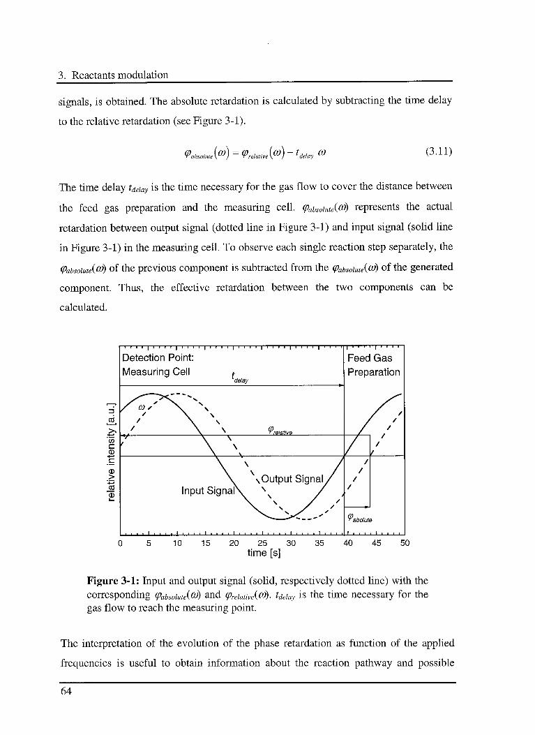
3. Reactants modulation
signals, is obtained. The absolute retardation is calculated by subtracting the time delay
to the relative retardation (see Figure 3-1).
(Pabsolutei®) = (Prelate) ~ l'delay « (3.11)
The time delay tdeiay is the time necessary for the gas flow to cover the distance between
the feed gas preparation and the measuring cell. (pabsoiute{co) represents the actual
retardation between output signal (dotted line in Figure 3-1) and input signal (solid line
in Figure 3-1) in the measuring cell. To observe each single reaction step separately, the
Çabsoiute{oi) of the previous component is subtracted from the cpabsoiute{(à) of the generated
component. Thus, the effective retardation between the two components can be
calculated.
•f | l l l I | l l l l [ i i i i | l l l l | l l 1 l |
Detection Point:
Measuring Cell
Figure 3-1: Input and output signal (solid, respectively dotted line) with the
corresponding (pabsoiute{oi) and cpreiative{co)- tdeiay is the time necessary for the
gas flow to reach the measuring point.
The interpretation of the evolution of the phase retardation as function of the applied
frequencies is useful to obtain information about the reaction pathway and possible
64
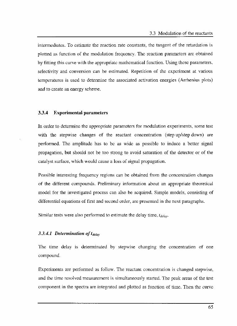
3.3 Modulation of the reactants
intermediates. To estimate the reaction rate constants, the tangent of the retardation is
plotted as function of the modulation frequency. The reaction parameters arc obtained
by fitting this curve with the appropriate mathematical function. Using these parameters,
selectivity and conversion can be estimated. Repetition of the experiment at various
temperatures is used to determine the associated activation energies (Arrhenius plots)
and to create an energy scheme.
3.3.4 Experimental parameters
In order to determine the appropriate parameters for modulation experiments, some test
with the stepwise changes of the reactant concentration (step up/step down) are
performed. The amplitude has to be as wide as possible to induce a better signal
propagation, but should not be too strong to avoid saturation of the detector or of the
catalyst surface, which would cause a loss of signal propagation.
Possible interesting frequency regions can be obtained from the concentration changes
of the different compounds. Preliminary information about an appropriate theoretical
model for the investigated process can also be acquired. Simple models, consisting of
differential equations of first and second order, are presented in the next paragraphs.
Similar tests were also performed to estimate the delay time, tdeiay
3.3.4.1 Determination of tdeiay
The time delay is determinated by stepwise changing the concentration of one
compound.
Experiments are performed as follow. The reactant concentration is changed stepwise,
and the time resolved measurement is simultaneously started. The peak areas of the test
component in the spectra are integrated and plotted as function of time. Then the curve
65
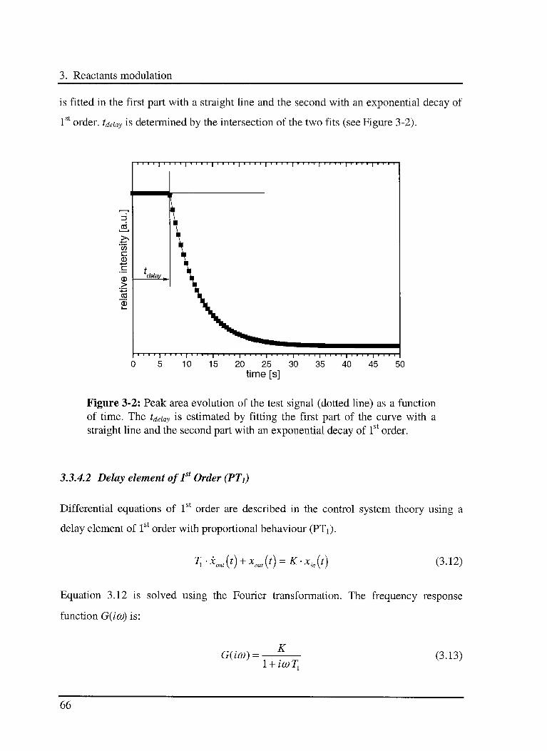
3. Reactants modulation
is fitted in the first part with a straight line and the second with an exponential decay of
1st order, tdeiay is determined by the intersection of the two fits (see Figure 3-2).
Figure 3-2: Peak area evolution of the test signal (dotted line) as a function
of time. The tdeiay is estimated by fitting the first part of the curve with a
straight line and the second part with an exponential decay of 1st order.
3.3.4.2 Delay element of 1st Order (PTi)
Differential equations of Is order are described in the control system theory using a
delay element of 1st order with proportional behaviour (PTi).
Tr-x0Ut{t) + x0Ut(t) = K-xm{t) (3.12)
Equation 3.12 is solved using the Fourier transformation. The frequency response
function G{ico) is:
G{ico) =K
1 + icoTi(3.13)
66
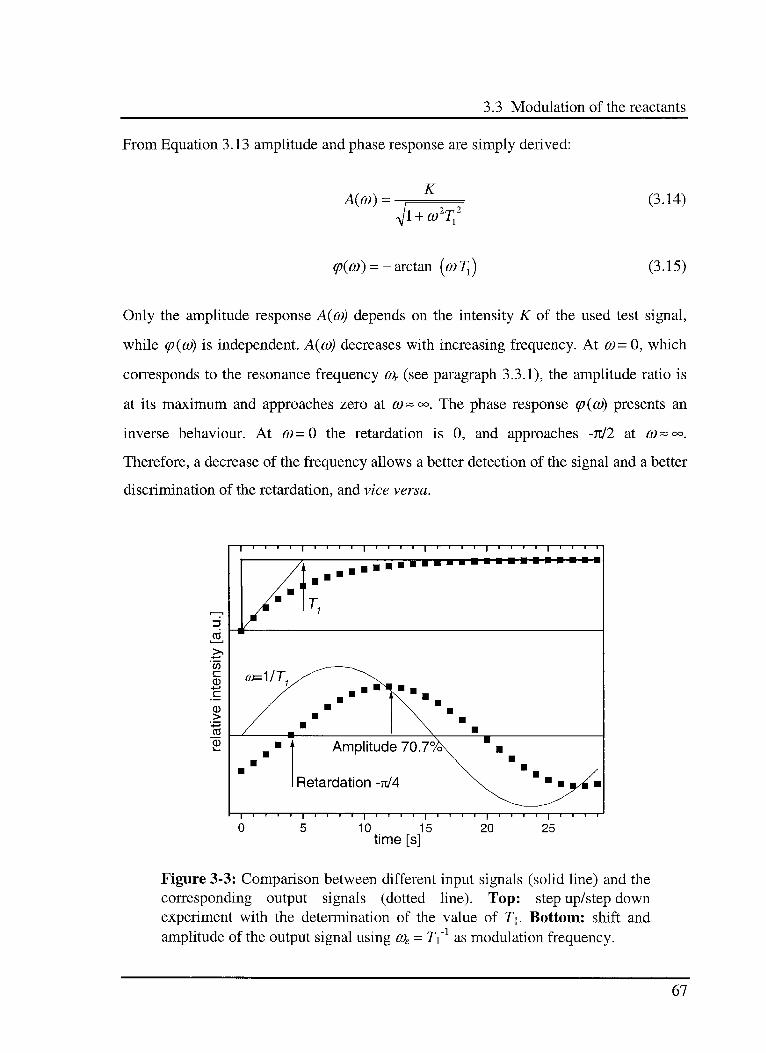
3.3 Modulation of the reactants
From Equation 3.13 amplitude and phase response are simply derived:
A{co) =K
yjl + C02T2(3.14)
(p{co) = - arctan (o)Tx) (3.15)
Only the amplitude response A{co) depends on the intensity K of the used test signal,
while (p{co) is independent. A{co) decreases with increasing frequency. At ü)=0, which
corresponds to the resonance frequency COr (see paragraph 3.3.1), the amplitude ratio is
at its maximum and approaches zero at co~°°. The phase response cp{oi) presents an
inverse behaviour. At co=0 the retardation is 0, and approaches -7t/2 at co~°°.
Therefore, a decrease of the frequency allows a better detection of the signal and a better
discrimination of the retardation, and vice versa.
d
7",
V)c
CD-1—•
c
CD>-t—>
<o=VTiys^
/ m
/ m
f\""\\\
m
mm
m
Amplitude 70.7°^"
\\
Retardation -n/4 \. m,V
(
i i i i
) i
1
10
tirr15 20 25
e[s]
Figure 3-3: Comparison between different input signals (solid line) and the
corresponding output signals (dotted line). Top: step up/step down
experiment with the determination of the value of T\. Bottom: shift and
amplitude of the output signal using coe = T{1 as modulation frequency.
67
3. Reactants modulation
The characteristic parameter of the considered delay element is obtained as follows.
From the plot of a step up/step down experiment, T\ is estimated (see Figure 3-3, top).
Using the same amplitude K of the step up/step down experiment and the Edge
Frequency coe - T{1 as modulation frequency, the intensity of the obtained signal should
be equal to 2"°'5 (=71%) of the step up/step down experiment, and a retardation of -%IA
should be observed (see Figure 3-3, bottom). Note that the PTi acts as a low pass filter,
and that the chosen frequency^ is equivalent to the bandwidth frequency cot (see
paragraph 3.3.1).
For the determination of the interesting frequency region some considerations are
necessary. As explained above, an increase in the frequency reduces the general quality
of the signal, and, at the edge frequency coe, the amplitude of the output signal is reduced
by = 30%. A retardation of -n/4 should already be achieved. To avoid the collection of
data having a large uncertainty the analysed region should be between the edge
frequency and co= 0.
nd3.3.4.3 Delay element of2 Order (PT2)
-.ndThe differential equations of 2 order are described in the control system theory using a
Mid
delay element of 2 order with proportional behaviour (PT2).
T22 KuM + ?! • *„,(') + xout{t) = K xjt) (3.16)
Equation 3.16 is solved using the Fourier transformation. The frequency response
function G{ico) is:
G{ico) = —— (3.17)l + icoT.-co-T2
From Equation 3.17 amplitude and phase response are quickly derived.
68
3.3 Modulation of the reactants
A{co) = -r=K
= (3.18)
^j{\-co2T2)2 + co2T2
cp{co) = - arctan
fcoT,
^
yl-C02T2j(3.19)
As for the PT], the phase response^ {co) is independent from the intensity K of the input
signal, but reveals an interesting evolution. At co - 0 the retardation is 0 and at co~ °°
cp{co) approaches 0, too. A similar behaviour of the retardation can be explained by
considering the PT2 element as two separate, consecutive PTi elements. Using high
frequencies both retardations approach the maximum value of -7i/2. Hence, at co~ °° the
total retardation is closer to -%. At co- T2A the total retardation approaches -n/2, and a
discontinuity is created. This last frequency is called Eigen Frequency C0q of the
undamped oscillation.
A{co) presents a more complicated evolution than for the delay element of 1st order. At
co~ c° the amplitude ratio approaches zero. The maximum value of A{co) depends on the
ratio Ti/T2. If this ratio is greater or equal to 20'5 then the amplitude has its maximum at
co= 0. In the other case A{co) reaches its maximum at the resonance frequency C0rm.
»^•f| <3-20)
and the corresponding amplitude ratio A{C0r) in given in Equation 3.21.
A{cor) = ^== (3.21)
T2 V AT2
69
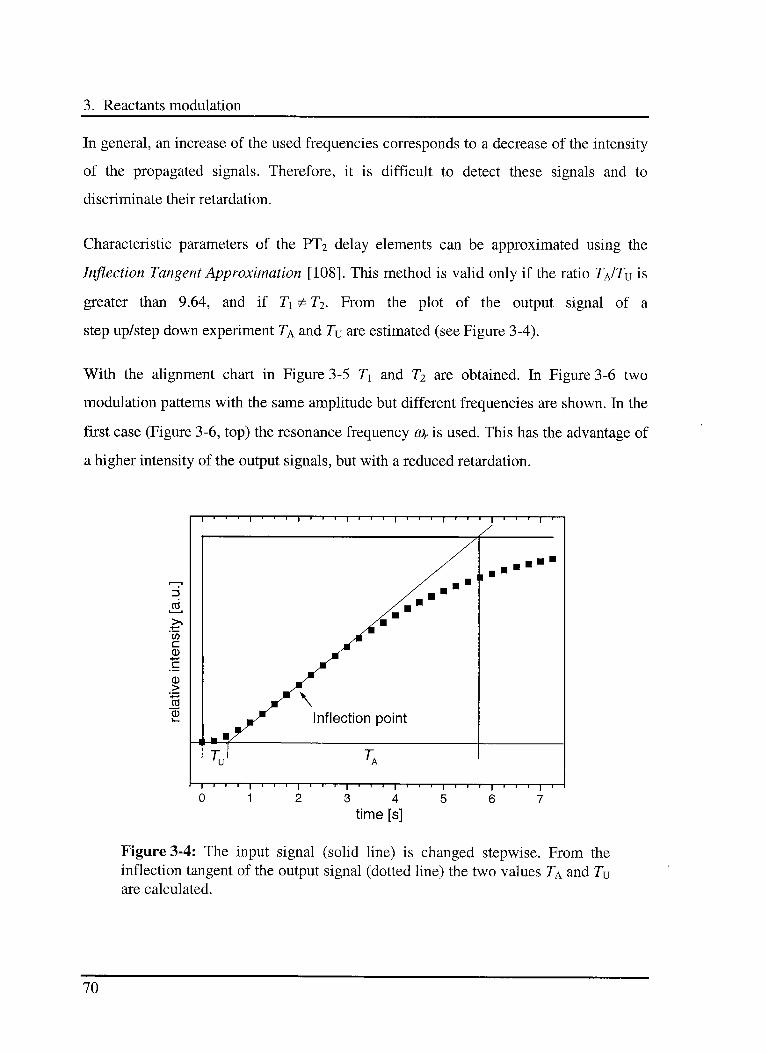
3. Reactants modulation
In general, an increase of the used frequencies corresponds to a decrease of the intensity
of the propagated signals. Therefore, it is difficult to detect these signals and to
discriminate their retardation.
Characteristic parameters of the PT2 delay elements can be approximated using the
Inflection Tangent Approximation [108]. This method is valid only if the ratio TpJTu is
greater than 9.64, and if T\ * T2. From the plot of the output signal of a
step up/step down experiment T& and 7\j are estimated (see Figure 3-4).
With the alignment chart in Figure 3-5 T\ and T2 are obtained. In Figure 3-6 two
modulation patterns with the same amplitude but different frequencies are shown. In the
first case (Figure 3-6, top) the resonance frequency COr is used. This has the advantage of
a higher intensity of the output signals, but with a reduced retardation.
1 1 1 1 1 1 1 1 1 1 1 1 1 1 1 1 1 1 1 1 1 1 1 1 1 1 1 1
/
6
cCD
Ç
CD>
CO y\CD
I--/
' Inflection point
1 1 1 1 —1—1—| 1 1—r—|—r—1—1—r—1—1 ! | 1 1 1 1 1 1 1 1
0 12 3 4 5 6 7
time [s]
Figure 3-4: The input signal (solid line) is changed stepwise. From the
inflection tangent of the output signal (dotted line) the two values Ta and 7\j
are calculated.
70
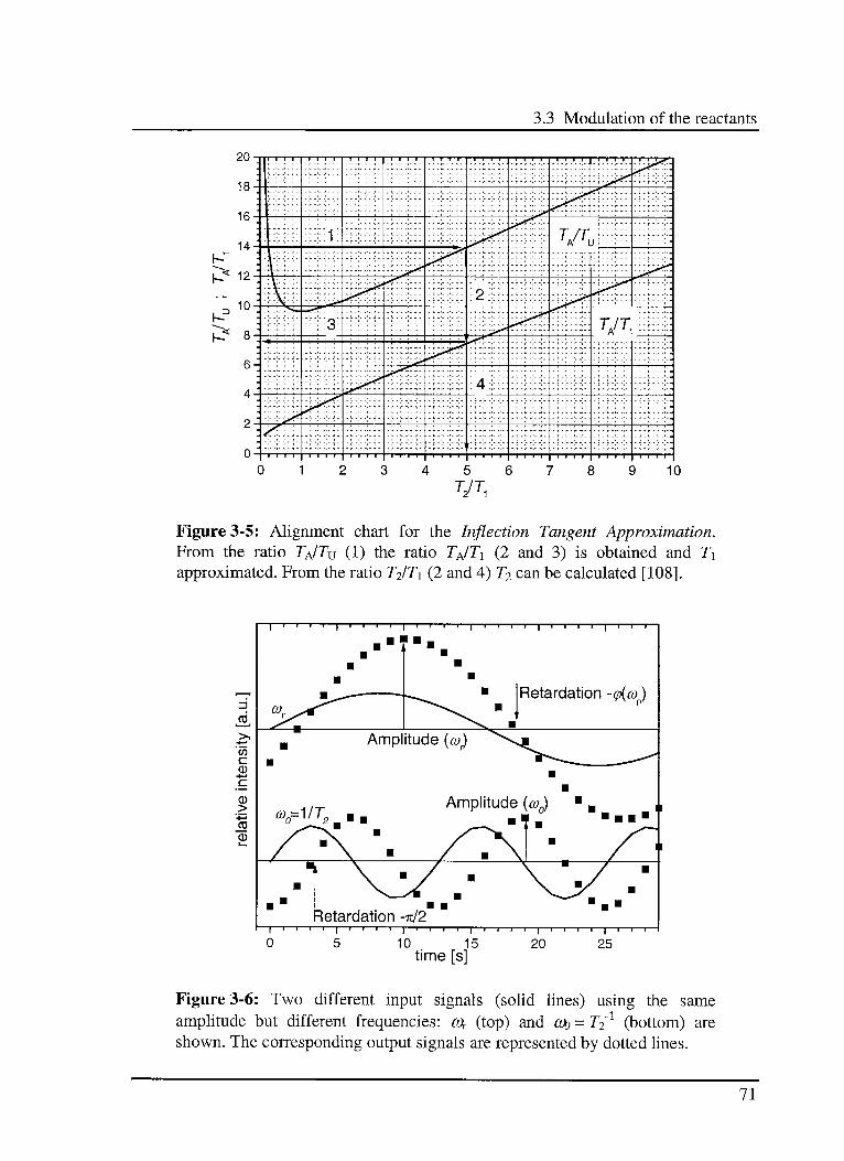
3.3 Modulation of the reactants
20
18
16
14
K* 12-i
K"10
8
\
:- \
\ '
1 T /TJ
\
\ ;\ \ ^
\ -
, ; 2 , . :
\_ .
3r V^
-*
; ;' :
:
^^ 4 \
; ;' '
: : ;•
: :
II 1 1 —i irr1 r r i i'
1 1 1 1 1
r
1111
1
1 1 1 1 i i i i I i i i i i i i i 1 1 1 1
0123456789 10
Figure 3-5: Alignment chart for the Inflection Tangent Approximation.From the ratio T/JTy (1) the ratio TpJT\ (2 and 3) is obtained and T\
approximated. From the ratio T2IT\ (2 and 4) T2 can be calculated [108].
| i i i . , i i i 1 I 1 1 | 1 I I T | 1 1 1 1 | 1 1 1
^ ^" Retardation -<p(co )
3CO ^^-"""^ "*"->.
p
Ä '^s^
u
~
Amp itude {co) "\jcoc *
—. ..
—~~^o
c
CD>1—'
CO
.,_ Amplitudeao=VT2a'm m
H) H
-_ _
i
_
CD/ X / X
/ \ / \ / i
*[ \ / \ ./ "
m v ^ ^ y^-^.. ^^-. -
Retardation -n/2—|—i—i—i—i—|—i—i—i—i—]—i—i—r—i—|—i—i—i—i—|—i—i—i—i—i—i—i—i—
10 15
time [s]
Figure 3-6: Two different input signals (solid lines) using the same
amplitude but different frequencies: co, (top) and coj = T2A (bottom) are
shown. The corresponding output signals are represented by dotted lines.
71
3. Reactants modulation
In the second case (Figure 3-6, bottom) the Eigen Frequency C0q is used, and the
expected retardation approaches -7t/2.
The determination of the interesting frequency region is not quite simple. As explained
above, an increase of the frequency lowers the general quality of the signal, but is
necessary to induce the oscillation of the PTi delay term elements included in the
investigated PT2. Therefore, analysis of the characteristic values: COq, cor and c% of the
system is necessary.
As rule of thumb, a region around the Eigen Frequency coj down to co- 0 is used as
starting point. This has the advantage that a retardation (-Tt/2), covering one half of the
maximum, has already been achieved.
3.3.5 Recording techniques
Experimental data are recorded using time resolved FTIR spectroscopy
[109,110,111,112,113]. Essentially, there are two time resolved FTIR techniques,
depending on the method used for moving the interferometer mirror: continuous moving
(slow-scan [110,114] respectively rapid-scan [115,116]) or step-by-step moving
(step-scan [117,118]).
In the slow-scan mode complete interferograms are recorded and immediately Fourier
transformed before starting the collection of a new spectrum. In the rapid-scan mode
sets of complete interferograms are collected before executing the Fourier
transformation. In both cases the co-addition of complete interferograms allows an
achievement of the desired Signal-to-Noise Ratio (SNR).
The slow-scan and rapid-scan technique are suitable to investigate reactions that occur
in the second to milliseconds range.
72
3.3 Modulation of the reactants
In the step-scan mode the interferograms are created point by point. At each mirror
position, data are collected for as long as it is necessary to achieve the desired SNR.
Then the mirror is moved to the next position, the experiment is repeated and new data
are collected. Using the accumulated data interferograms the Fourier transformation is
performed.
Step-scan is useful for reactions in the microseconds to nanoseconds range. Due to the
necessity of repeating each single experiment at each mirror position the investigated
processes should be easily repeated to avoid long measurement times, examples are:
photoacustic spectroscopy [119,120], liquid crystal reorientation [121] and
photo-excited states investigation [122].
3.3.6 Recording parameters
Independently from the applied recording technique it is not easy to achieve a high
enough SNR for plausible spectra. The SNR value can be controlled by the aperture,
filters, resolution, scan velocity and number of collected spectra.
Modification of the aperture and used filters is a simple way to improve the SNR. The
used parameters should allow the highest energy throughput, but any limitation of the
collected frequency windows should be avoided. Scan velocity, resolution and number
of averaged scans have a strong influence on the SNR. The number of photons reaching
the detector should be as high as possible. The scale of the spectra and the time
resolution should allow the evaluation of the observed retardation. To find the best
condition test experiments are necessary.
73
3. Reactants modulation
3.4 Useful simple models
3.4.1 A few definitions in heterogeneous catalysis
A reaction is heterogeneous if it requires the presence of at least two phases to proceed
at the given rate. Since more than one phase is present, the movement of material from
phase to phase must be considered.
A central problem is the reaction pathway. In systems, such as solid catalysed reactions,
where several series-parallel reactions are usually present, the concentration of the
different intermediates is usually difficult to determine. To overcome this problem, rates
are expressed in terms of overall reaction rates {roveraii). These are absolute rate
expressions of the whole reaction, or of a single reaction step. Additionally to the usual
chemical kinetics terms, mass transfer terms are also incorporated.
If the changes take place by parallel paths, under steady state conditions the overall rate
is simply the sum of all individual rates (r,).
n
overall = E r« ^2T>
On the other hand, if the overall change requires that a number of steps take place in
succession, at steady state, all these steps will proceed at the same rate.
Overall = Cl (3"23)
In this case the step providing the major resistance is called rate-limiting step, and can
be considered alone. In Equation 3.24 the nth order reaction of compoundA is shown.
r =k -A" (3.24)overall icite-hmiting
;
1A
3.4 Useful simple models
This procedure leads to a very simple expression and is used whenever possible. More
details about the modelling and the design of chemical reactions can be found m the
literature [123,124].
3.4.2 Heterogeneous reactions in the used setup
As explained above, both used setup can be modelled as a continuous stirred tank
reactor with residence time r. The difference between the two setup can be summarised
in the following way. The DRIFT cell permits the observation of gas phase and surface
composition, but has a lower sensitivity towards the gas phase. The u,-reactor/gas cell
system has a high sensitivity for gases, but no surface species can be detected.
Therefore, a reduced amount of information can be collected and only suggestions about
the reaction pathways can be obtained.
The gas cell acts as a continuous stirred tank that induces a supplementary retardation of
each monitored compound. The retardation of a compound A can be represented using
the following differential equation-
~~7~= ~TIR-cell A + riR-cell A) (3.25)
where Ao is the concentration of A m the entering the gas cell from the reactor side, and
% ceil is the residence time m the cell. The equation is resolved using the Fourier
transformation (see Equation 3.3), and the retardation as a function of co is obtained.
tm(cpA-çAi) = coTIR_ceU (3.26)
As expected the cell causes a retardation of the signals, which is only function of the
residence time The use of faster gas flows allows to reduce this value.
75
3. Reactants modulation
In the following paragraphs several simple models are presented and discussed. The
reactions start always with compound A, with a concentration of A» in the feed gas. All
the reaction rate constants £, are considered as overall first order rate constants.
3.4.2.1 Adsorption/'desorption equilibrium
The adsorption of a component is the first step in each catalysed reaction, while the
desorption always follows. Knowledge about these equilibria is of great interest for an
understanding of observed reaction behaviour, as well as in the formulation of plausible
reaction schemes.
In this paragraph the equilibrium between an adsorbate B* and a gas phase component
A is considered. If a low partial pressure is applied, the surface concentration of vacant
adsorption sites can be assumed as constant, and the following simple model can be
used:
A^^B*
A^-B*
The system is described using the following set of differential equations.
dA— = -{kx + -r1 )A + r~l\ + k2B *
dt(3.27)
dB*= -k2B * +kxA
dt
This set of differential equations is solved using the Fourier transformation. The
retardation as function of co is obtained.
tan
, xcoico2 + Lk, +k2)
76
3.4 Useful simple models
tan(ç?s„ -çA) = cok2 (3.29)
For B*, the retardation is only dependent on the desorption reaction. For A, a
superposition is present. Considering that co2 is only important when high frequencies
are applied, a low frequency approximation can be used.
tan(ç?A -cpA = corik^k'1 +1) (3.30)
In this approximation the reaction rates are substituted by an overall equilibrium
constant {k\/k2). The single values can be obtained using the value for k2 estimated in
Equation 3.29. If the residence time approaches zero, the retardation of A approaches
zero too, and only the retardation of B* can be monitored. A minor desorption or
adsorption indicates a surface saturated with stable species. Therefore, the system acts
as simple continuous stirred tank.
3.4.2.2 Series reactions
Series reactions consist of a sequence of two or more reaction steps. These represent the
simplest form of catalytic reactions, where only one end product is formed.
In the considered system a compound A adsorbs on the surface to form B*, which reacts
to the end product C If a low partial pressure ofA is used, the surface concentration of
vacant adsorption sites can be considered as constant. The use of an excess of other
involved components allows the assumption of constant surface concentration. The
following simplified model is used:
A h >B* h )C
which is described by the following set of differential equations:
77
3. Reactants modulation
^ = -(^1+r-1)A + T-1Aûdt
dB*^— = -k2B*+kxA (3.31)dt
— = -T~lC + k2B*
dt2
The system is resolved using the Fourier transformation and the retardation is expressed
as function of co.
tan(pA -<pAo) = <o(kl + r-'Y (3.32)
tan(<pB„ -cpA) = cok21 (3.33)
tan(^c -<pB*) = cot (3.34)
For A and B* the retardation is influenced by the adsorption and the reaction. For C only
the residence time is important. The use of small residence times induces the retardation
ofA and C to approach zero. The only remaining retardation is given by Equation 3.33.
3.4.2.3 Parallel reactions
For parallel reactions, two or more reaction steps originate from the same intermediate,
but different end products are obtained. Similar models are used for the case that
expected as well as undesired products are generated from the same intermediate.
In the chosen example the compound A adsorbs on the surface, and the adsorbate B* is
created. This reacts to the end products C and D. As discussed in the previous
paragraph, the use of an excess of other involved components and a low partial pressure
ofA lead to the following simple model.
78
3.4 Useful simple models
B* kl >C
B ->£>
This model is described by the following set of differential equations:
~ = -{kl+T-1)A + T-1A0dt
dB'= -{k2+k3)B*+k,A
dt
— = -T-lC + k2B*
dt2
— = -T~lD + kzB*
[dt3
(3.35)
The set is solved and the solution is given as function of the modulation frequency.
tan(^-^Ao) = c;(r-1+^1)"1 (3.36)
tan(çjBt-q}A) = œ(k2 + k3)~
tan(#7c -<pB>) = cot
tan(cpD - cpBt) = co t
(3.37)
(3.38)
(3.39)
As expected, the retardations of compounds A and B* depend on the rates of the
different reaction steps. End products C and D present the same retardation, which is
only dependent on the residence time. If r approaches zero, all gas phase species show
no retardation any longer, and only Equation 3.37 remains valid.
3.4.2.4 Series-parallel reactions
In series-parallel reactions different reaction steps, both in series and in parallel, are
present. These represent the classical situation in heterogeneous catalysis. A reactant can
79
3. Reactants modulation
generate different products and intermediates, which can lead to various other end
products.
In the considered example the compound A adsorbs on the surface to form B*, which
can either react to the end product C or to the intermediate D. The last component reacts
to a separate intermediate E* that further leads to the end product F. If all the previously
discussed simplifications about surface concentration of vacant adsorption sites and
co-reactants are valid, the following simplified model can be used.
A—^5*^^->C
B* *3 >D ki >E*—^—>F
The system is described using the following set of differential equations:
dA_dt
dB*
dt
dC
dt
dD
dt
dE*
-{kl+r-l)A + T~1A0
= -{k2 + k3)B*+kxA
= -r^C + KB-
^ = -{k4 + T~1)D + k3B*
= -k5E*+kADdt
dF_dt
-T~lF + kKE *
(3.40)
The solutions as function of co are the following:
tm(<pA-<pAo) = a)(T-1 + kl)~1
tan(<?v - cpA) = co(k2 + £3)_1
tan(^7c -<pBY) = cot
(3.41)
(3.42)
(3.43)
80
3.4 Useful simple models
tan(<pD - (pg.) = co (r~l + £4)*
(3.44)
itm(cpE,-cpD) = cok~x (3.45)
im(cpF -çe*) = cot (3.46)
As expected, the retardations of the compounds A and D depend on both, reaction and
residence time. The retardation of the intermediates {B* and E*) and of the end products
(C and F) depends only on the reaction rates and only on the residence time,
respectively. Due to the consecutive reaction, D precedes C in phase. If k^ approaches
zero the two compounds, C and D, would present the same retardation. If T approaches
zero only Equations 3.42 and 3.45 remain valid, because all other retardations approach
zero.
An amazing situation is possible if C and F represent the same end product. In this case,
in Equations set 3.40 F disappears and the differential equation for C is:
— = -T~lC + k2B*+k5E* (3.47)dt
that yields the following solution:
tan(pc-$v) =
coTlkJco2 + k2^j (co2t2 +(k4T + lf) + k3k4k5(kAT + 2k5T + l + k4ksT2 -oj2t2)) (3.48)
kJco2 +ft52) (co2t2 + (k4T + lf\ + k3kiksT(k5(l + k4T)-co2T(2 + k4T-k5T))
The signal of C is obtained from a superposition of two signals, the first is generated
from B* and the second from D*. The retardation is placed between the two limits. The
lower limit is given by k3 ~ 0, where the solution corresponds to Equation 3.43. The
upper limit is given by k2 ~ 0, where the solution is obtained from Equation 3.49. This
corresponds to the retardation between B* and F as given in the Equations set 3.40.
81
3. Reactants modulation
co (k4T + 2k5T +1 + k4k5T2 - co2T2)tan{<pF -cpBA-
^ +^ _^^+ ^T_ ^T)(3.49)
In the case of a residence time approaching to zero, Equation 3.48 is mainly dependent
on the value of k2. To show this relationship better, Equation 3.48 is rewritten with new
variables {X, Y and Z) and isolating r.
tan(çc - p») =
co(k2X + Y)X^z
X T— +—
(3.50)
v2 7
The new variables X, Y and Z are defined in the Equations set 3.51. The ratio Tlk2 is very
important, because from the residence time indications about k2 can be drawn directly. If
t approaches zero, the expected retardation approaches zero too. An observed large
value of the retardation indicates that k2 approaches zero, too.
X = (co2 + k2 ) (co2t2 +(k4T +1)2
Y = k3k4k5(k4T + 2k5T +1 + k4ksT2 - co2T2\
Z = k3k4kJk5(l + k4T) - co2t(2 + k4T - k5T))
(3.51)
3.5 Conclusions
The information potential of the reactants modulation technique in FTIR/DRIFT
spectroscopy studies of heterogeneous catalysis has been described. The experimental
procedure and the selection of the experimental conditions were discussed.
Some simple situations have been worked out to exemplify how this technique can be
used to yield kinetic information and hints on reaction pathways. Equations were
82
3.5 Conclusions
derived to show the relationship between the retardation of the concentration waves and
the system parameters, such as reaction rate constants and residence time. All these
parameters can be calculated from the experiments without the necessity of previously
established calibration curves.
83
This is page 84 !
This page was left intentionally blank !
4.1 Introduction
4. Reaction pathway investigation
4.1 Introduction
In this chapter the modulation concept for the investigation of the reaction pathways is
presented. The induced dynamic changes in the concentrations of products,
intermediates and reactants were monitored by FTIR spectroscopy in the gas cell. The
observed phase retardation A<p between the external perturbation of the feed gas and the
signals of products, intermediates and reactants was studied depending on the
modulation frequency co.
The methanol synthesis from CO/C02fH2 over a commercial Cu/ZnO/A^Os catalyst
was selected. Further details on the application of the modulation concept on this system
can be found elsewhere [125,126]
Methanol is a key compound in the chemical industry and a suitable energy carrier. It is
the precursor of several other widely used chemicals, such as formaldehyde, acetic acid,
MMA (methyl-methacrylate), DMT (dimethyl-terephthalate), MTBE (methyl-tertiary-
butylether) and chloromethanes.
The application of methanol as fuel is very important. It can either be used in
combustion engines, or partially oxidised to yield C02 and hydrogen, which is used in
fuel cells. Methanol has twice the energy density of liquid hydrogen, but without the
storage and transport problems. In the Rio de Janeiro agreements (1992) and Kyoto
protocols (1997) the attendees agreed to notably reduce the emission of greenhouse
85
4. Reaction pathway investigation
gases to the atmosphere in the next decade. The methanol synthesis starting from C02
appears to be a valid approach to lower the release of this gas to the environment.
Since the introduction of highly selective Cu/ZnO catalysts by ICI in 1960s, the
industrial production of methanol is exclusively based on this technology. All currently
used catalysts contain copper oxide and zinc oxide with one or more stabilising
additives, mainly AI2O3 and graphite. In the past years numerous investigations were
carried out to clarify the various aspects of the reactions involved in the methanol
synthesis, and different views of the mechanism have been proposed [127,128,129,130].
For the investigated system Ovesen et al. [131,132,133] and Askgaard et al. [134] have
demonstrated that the water-gas shift/reverse water-gas shift reactions are taking place
via adsorbed CO and C02 respectively. The hydrogénation reaction starts from adsorbed
CO2 and leads, via formates and methoxy, to the methanol product.
4.2 Experimental
The used setup consists of the gas dosing system Modulation Unit, described in section
2.3.2, which is attached to the (X-reactor/gas cell system (see section 2.5). All spectra
were recorded in the rapid scan mode with a resolution of 4 cm"1 and an accumulation of
8 to 64 interferograms for the time dependent spectra, and 1024 scans for background
spectra. The used FTIR spectrometer is presented in section 2.6.
A commercial CO/C02 hydrogénation Cu/ZnO/Al203 catalyst, kindly provided by
Haldor Tops0e A/S, was ground, sieved, and placed into the micro reactor. The reactor
length was adjusted to minimise the dead volume. The catalyst was activated by
reduction in 10%-H2/N2 with an overall flow of 2 1N min"1 at 5 bar using the following
temperature program: 3 K min"1 up to 453 K, and 1 K min"1 up to 523 K.
86
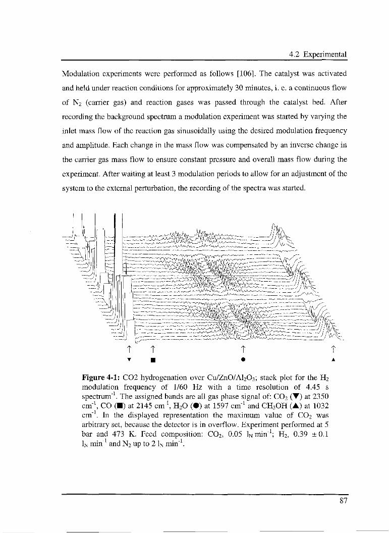
4.2 Experimental
Modulation experiments were performed as follows [106]. The catalyst was activated
and held under reaction conditions for approximately 30 minutes, i. e. a continuous flow
of N2 (carrier gas) and reaction gases was passed through the catalyst bed. After
recording the background spectrum a modulation experiment was started by varying the
inlet mass flow of the reaction gas sinusoidally using the desired modulation frequency
and amplitude. Each change in the mass flow was compensated by an inverse change in
the carrier gas mass flow to ensure constant pressure and overall mass flow during the
experiment. After waiting at least 3 modulation periods to allow for an adjustment of the
system to the external perturbation, the recording of the spectra was started.
T î t t
• a
Figure 4-1: C02 hydrogénation over Cu/ZnO/Al203; stack plot for the H2
modulation frequency of 1/60 Hz with a time resolution of 4.45 s
spectrum"1. The assigned bands are all gas phase signal of: C02 (T) at 2350
cm"1, CO () at 2145 cm"1, H20 (•) at 1597 cm"1 and CH3OH (A) at 1032
cm".In the displayed representation the maximum value of C02 was
arbitrary set, because the detector is in overflow. Experiment performed at 5
bar and 473 K. Feed composition: C02, 0.05 lNinin"1; H2, 0.39 ±0.1
In min"1 and N2 up to 2 1N min"1.
87
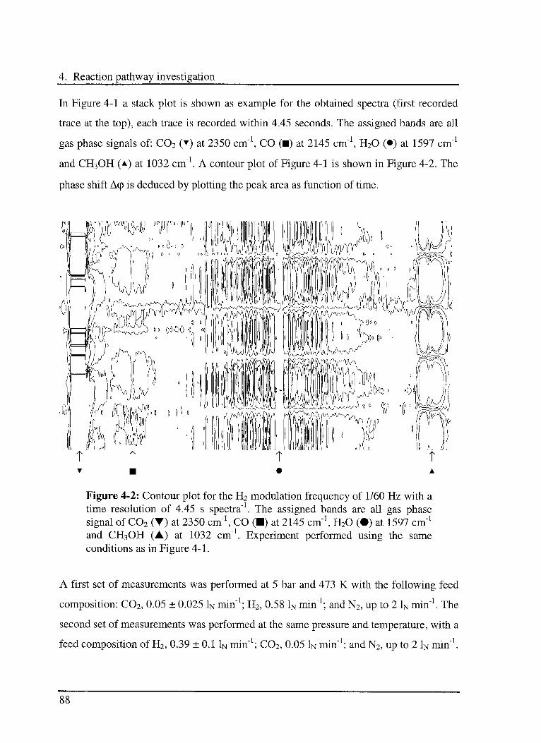
4. Reaction pathway investigation
In Figure 4-1 a stack plot is shown as example for the obtained spectra (first recorded
trace at the top), each trace is recorded within 4.45 seconds. The assigned bands are all
gas phase signals of: C02 () at 2350 cm"1, CO () at 2145 cm"1, H20 (•) at 1597 cm"1
and CH3OH (a) at 1032 cm"1. A contour plot of Figure 4-1 is shown in Figure 4-2. The
phase shift A(p is deduced by plotting the peak area as function of time.
Figure 4-2: Contour plot for the H2 modulation frequency of 1/60 Hz with a
time resolution of 4.45 s spectra"1. The assigned bands are all gas phasesignal of C02 (T) at 2350 cm"1, CO () at 2145 cm"1, H20 (•) at 1597 cm"1
and CH3OH (A) at 1032 cm"1. Experiment performed using the same
conditions as in Figure 4-1.
A first set of measurements was performed at 5 bar and 473 K with the following feed
composition: C02, 0.05 ± 0.025 1N min"1; H2, 0.58 1N min"1; and N2, up to 2 1N min"1. The
second set of measurements was performed at the same pressure and temperature, with a
feed composition of H2, 0.39 ± 0.11N min"1; C02, 0.05 1N min"1; and N2, up to 2 1N min"1.
88
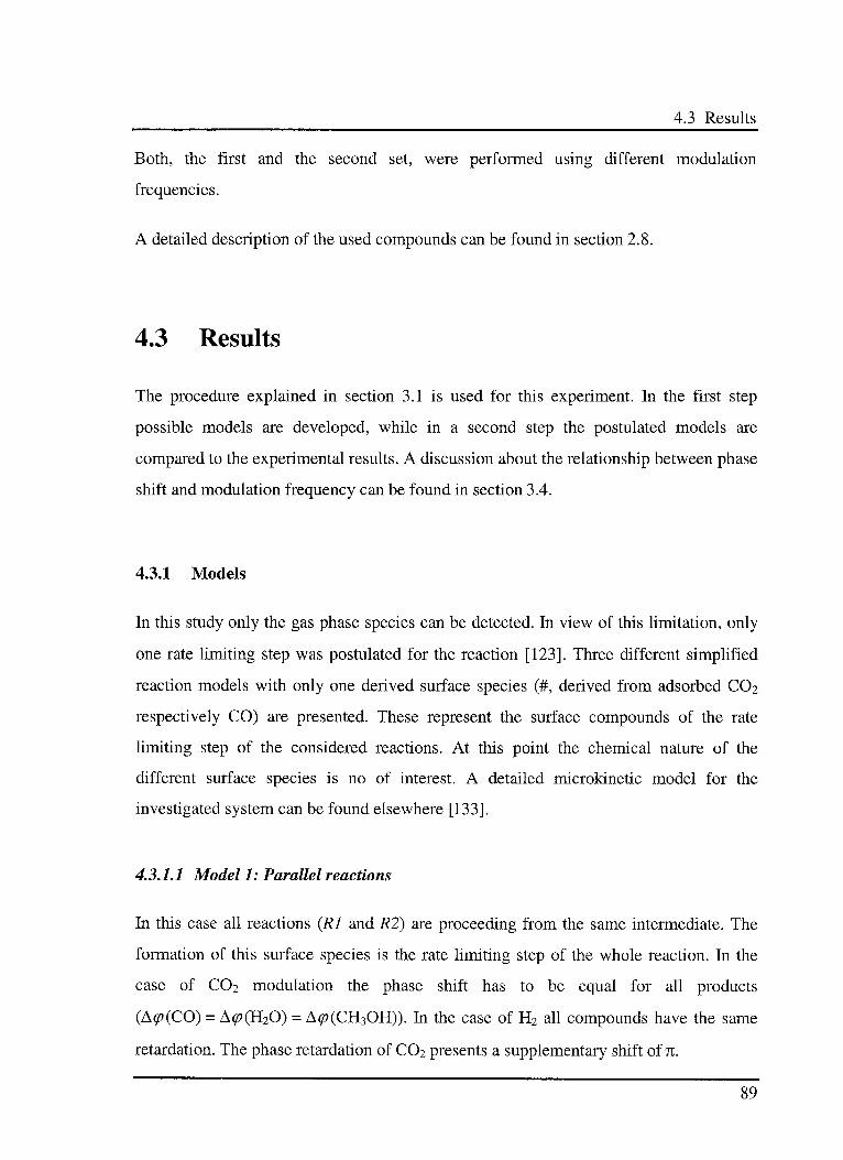
4.3 Results
Both, the first and the second set, were performed using different modulation
frequencies.
A detailed description of the used compounds can be found in section 2.8.
4.3 Results
The procedure explained in section 3.1 is used for this experiment. In the first step
possible models are developed, while in a second step the postulated models are
compared to the experimental results. A discussion about the relationship between phase
shift and modulation frequency can be found in section 3.4.
4.3.1 Models
In this study only the gas phase species can be detected. In view of this limitation, only
one rate limiting step was postulated for the reaction [123]. Three different simplified
reaction models with only one derived surface species (#, derived from adsorbed CO2
respectively CO) are presented. These represent the surface compounds of the rate
limiting step of the considered reactions. At this point the chemical nature of the
different surface species is no of interest. A detailed microkinetic model for the
investigated system can be found elsewhere [133].
4.3.1.1 Model 1 : Parallel reactions
In this case all reactions {Rl and R2) are proceeding from the same intermediate. The
formation of this surface species is the rate limiting step of the whole reaction. In the
case of CO2 modulation the phase shift has to be equal for all products
(Ac? (CO) = A#?(H20) = Aç?(CH3OH)). In the case of H2 all compounds have the same
retardation. The phase retardation of C02 presents a supplementary shift of n.
89
4. Reaction pathway investigation
C02 -> [#] *2> CO + H20 {Rl)
C02 -> [#] —^-» CH3OH + H20 {R2)
4.3.1.2 Model 2: Series reactions
In this model methanol is produced in a second step from adsorbed CO {R3).
C02 -» [#]Ha
> CO + H20 (i?i)
CO -> [#] 2H?) CH3OH {R3)
During C02 modulation the phase shift H2O/CO2 and CO/CO2 from the reverse water
gas shift reaction should be the same.
However, if CO has to be consumed to obtain methanol, its absolute phase shift must be
smaller than the one of H20. Methanol is at the end of the reaction sequence; however,
if its formation from CO is sufficiently rapid, its phase shift may lie between those of
CO and H20 (Ap(CO) < [ A<p(H20) or A<p(CH3OH) ])•
During H2 modulation the phase shifts of CO/H2, H20/H2 and CH3OH/H2 should be
monitored together. If CO was consumed to produce methanol, the phase shift CO/H2
would be smaller and the phase shift CH3OH/H2 would be larger than the relative phase
shift of H2O/H2 (Ap(CO) < A^(H20) < Ap(CH3OH)). The phase shift of C02 would
present a shift of 7t with respect to the water signal.
4.3.1.3 Model 3: Series-parallel reactions
Here all three reactions presented so far are assumed to proceed simultaneously.
C02 -» [#] —2*-> CO + H20 (Rl)
C02 -> [#] —^-^ CH3OH + H20 (R2)
90
4.3 Results
CO -> [#] —2Jk~^ CH3OH (R3)
The case for CO2 modulation is similar to those of series reactions. The sequence of
absolute phase shifts will not be changed: Atp(CO) < [ A#>(H20) or A#>(CH3OH) ].
In case of H2 modulation, one might expect from visual inspection that all products have
the same phase shift. However, CO is used to produce methanol, and hence the phase
shift CO/H2 will be smaller and the phase shift CH3OH/H2 will be larger. The sequence
is again: Acp (CO) < Acp (H2O) < Ac (CH3OH), even though at the same time C02 is
directly reduced to CH3OH and water. This fact is not influencing the discussed result.
The phase shift CH3OH/H2 will be similar to the phase shift of H20/H2.
4.3.2 Experimental results
In this section the above presented models are discussed in relation to the observed
phase shifts to check the proposed pathways.
4.3.2.1 Modulation of CO2
In the present system C02 modulation induces a modulation of all following reaction
steps. As shown in Figure 4-3, the phase shifts H20/C02 and CH3OH/C02 are not the
same. The corresponding curves could be fitted with the phase function of a third order
delay term (PT3), suggesting more than one relevant surface species and/or several
reaction pathways leading to the same products [131,132,133,134].
CO is produced first (smallest phase shift) and the curve can be fitted with the phase
function of a second order delay term (PT2), suggesting that only one relevant surface
species was involved and that CO is reacting. In any case, even assuming that more
surface species are involved in model 1, water should exhibit a phase shift between
those of methanol and CO, because it can be produced from both reactions. This could
91
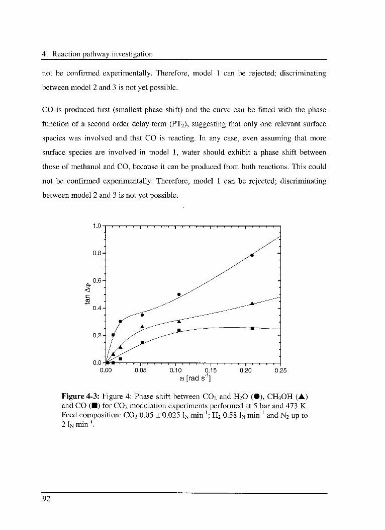
4. Reaction pathway investigation
not be confirmed experimentally. Therefore, model 1 can be rejected; discriminating
between model 2 and 3 is not yet possible.
CO is produced first (smallest phase shift) and the curve can be fitted with the phase
function of a second order delay term (PT2), suggesting that only one relevant surface
species was involved and that CO is reacting. In any case, even assuming that more
surface species are involved in model 1, water should exhibit a phase shift between
those of methanol and CO, because it can be produced from both reactions. This could
not be confirmed experimentally. Therefore, model 1 can be rejected; discriminating
between model 2 and 3 is not yet possible.
"I .0 I i 1 i 1 i i 1 i'r—
i"T"r"M,i' i1 "j 1 1 1 1 1 1 1 1 1—
0.8- ^S
0.6- /^9-
. /< /«= y^ ^
CO - ^^ .__—-"^4—» ^^ ^
0.4- ^^ _-—-~"^
0.2- 4 / ^^^
0.0 ! i ! i i—i , | i i 1 t | i . i—i 1—i 1 1 r—
0.00 0.05 0.10 0.15 0.20 0.25
co [rad s"1]
Figure 4-3: Figure 4: Phase shift between C02 and H20 (•), CH3OH (A)and CO () for C02 modulation experiments performed at 5 bar and 473 K.
Feed composition: C02 0.05 ± 0.025 1N min"1; H2 0.58 In min"1 and N2 up to
2 1N min"1.
92
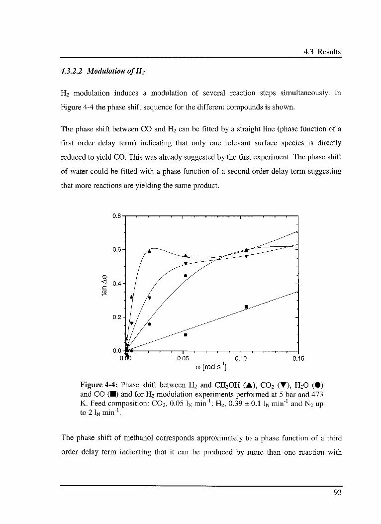
4.3 Results
4.3.2.2 Modulation ofH2
H2 modulation induces a modulation of several reaction steps simultaneously. In
Figure 4-4 the phase shift sequence for the different compounds is shown.
The phase shift between CO and H2 can be fitted by a straight line (phase function of a
first order delay term) indicating that only one relevant surface species is directly
reduced to yield CO. This was already suggested by the first experiment. The phase shift
of water could be fitted with a phase function of a second order delay term suggesting
that more reactions are yielding the same product.
0.8 —1 1 1 1 1 1 1 1 1 1 1 1 1 1 r
Figure 4-4: Phase shift between H2 and CH3OH (A), C02 (T), H20 (•)and CO () and for H2 modulation experiments performed at 5 bar and 473
K. Feed composition: C02, 0.05 1N min"1; H2, 0.39 ± 0.1 1N min"1 and N2 up
to 2 lNiriin"1.
The phase shift of methanol corresponds approximately to a phase function of a third
order delay term indicating that it can be produced by more than one reaction with
93
4. Reaction pathway investigation
several intermediates. From this information it is already possible to reject model 2 and
to select model 3 as the most reasonable among the choices considered.
4.4 Discussion
In the chosen model (3), CO2 reacts to yield CO via a derived surface species #, and CO
can react to yield CH3OH via the same derived surface species #. This is an alternate
way to consider the equilibrium between C02 and CO established via the water-gas
shift/ reverse water-gas shift reactions. The formation of derived surface species #
represents the rate limiting step intermediate in the hydrogénation of CO to methanol. If
CO was directly converted to CH3OH the retardation of C02 in Figure 4-4 would be
smaller than the relative phase shift of CO. Hence, it is possible to conclude that CO and
C02 are in equilibrium and that the reaction of CO to methanol occurs via C02.
This is in agreement with the microkinetic model that has been proposed for
Cu/ZnO/Al203 catalysts [131,132,133,134], in which CO and C02 are in equilibrium
via the water-gas shift reaction. The oxidation of adsorbed CO to adsorbed C02 is the
rate limiting step of this latter equilibrium.
The considered model (3) assumes that carbon dioxide reacts to methanol via a surface
species (#co2) derived from C02, where the rate limiting step is the reduction of this
species.
This is also in agreement with the previously mentioned microkinetic model in which
adsorbed C02 is hydrogenated to methanol via formates, and methoxy species
[131,132,133,134]. The formation of methoxy is the rate limiting step.
The experimental results are sufficient to create a simplified model for this system. An
extended version of model 3, including more surface species, has to be developed to
understand the reaction pathway in more detail.
94
4.5 Conclusions
4.5 Conclusions
The periodic modulations of reactant concentrations were used to induce time dependent
changes in the FTIR signals of reactant, intermediate, and products. These were
monitored to obtain information on the reaction pathway of methanol synthesis over
Cu/ZnO/Al203, where a series-parallel model was found to be most appropriate. This
proofs the validity of the modulation concept in heterogeneous catalysis as monitored by
FTIR.
95
This is page 96 !
This page was left intentionally blank !
5.1 Introduction
5. Reaction rate constants investigation
5.1 Introduction
In this chapter the application of the modulation concept for studies of the reaction rate
constant of solid-state catalysed reactions is presented. The dynamic variations in the
concentrations of products, intermediates and reactants are monitored in situ in a DRIFT
cell. The observed phase shift (Atp) is examined depending on the modulation frequency
co. This is used to derive the rate constants, characterising the single reaction steps, and
reaction orders. The repetition of experiments at different temperatures makes it
possible to calculate the temperature dependent constants.
The CO oxidation over a Pd25Zr75 based catalyst is studied in detail. Further details on
the application of the modulation concept on this system can be found elsewhere
[106,135].
Generally, the oxidation of carbon monoxide to C02 by oxygen is an efficient method to
remove highly diluted CO from gases. This is of practical importance for the treatment
of exhaust gases of internal combustion engines. The current state of technology of fuel
cells operating with the reformate gas of liquid fuel, e. g. gasoline and methanol,
demands high purity CO-free feed gases, because carbon monoxide acts as poison for
the electrocatalyst of the polymer electrolytes. The selective oxidation of CO in the H2
containing reformate is a suitable procedure.
The kinetics of the CO oxidation over Pd (or Pt) based catalysts exhibits a multifaceted
behaviour. Three characteristic regimes of the reaction rate can be distinguished. With
97
5. Reaction rate constants investigation
increasing CO partial pressure the reaction rate increases first linearly with CO partial
pressure, then an oscillating behaviour follows, and finally a quenched reaction state is
reached [136], in which the apparent order with respect to CO is negative.
A corresponding behaviour is reported for the reaction rate as a function of temperature.
While at low temperatures the reaction rate is of negative order for CO, it passes
through a range of oscillations with increasing temperature, and finally exhibits a linear
increase with CO partial pressure at high temperatures [137]. Evidence for a Langmuir-
Hinshelwood mechanism for the reaction on metal surface was reported by different
authors [106,138,139,140,141]. The oscillating behaviour of the reaction rate onto Pd
and Pt was intensively investigated [136,137,142,143,144,145,146].
The properties of the used PdZr catalyst have been investigated and discussed in detail
by Baiker et al. [147,148,149,150], Ladas et al. [142], and Barnickel et al. [151]. It was
found that oxygen atoms adsorb on the substochiometric zirconia (Zr02.x), whereas CO
molecules adsorb and are consecutively oxidised on the surface of the palladium
component. In a previous work on the same catalyst [125], the band at 2056 cm"1 was
assigned to CO linearly bound to Pd [151,152].
5.2 Experimental
The used setup consists of the gas dosing system Modulation Unit (see section 2.3,2)
attached to the DRIFT cell presented in section 2.4.2. The whole setup is controlled
using the program presented in section 2.2. The FTIR spectrometer is described in
section 2.6. All spectra were recorded in the rapid scan mode with a resolution of 4
cm"1. For transient measurements 8 to 32 interferograms per spectra and 1024 scans for
the background spectra were accumulated.
98
5.2 Experimental
The amorphous Pd^Zrys alloy catalyst for CO oxidation was prepared by the melt
spinning technique [153]. A given amount (0.306 g) of catalyst was placed in the
DRIFT sample cup and packed with a stamp using a pressure of 1 MPa to ensure
reproducibility [31].
The experiments were performed as follows. In a first step the dead time between the
gas dosing system (the mixing of the feed gas) and the cell was estimated with
step up/step down experiments (see paragraph 3.3.4.1). In a second step the modulation
experiments were started. To monitor the influence of the temperature on the reaction,
the experiment was repeated applying different temperatures. The changes of
concentrations in step up/step down and modulation experiments have the same order of
magnitude.
Step up/step down and modulation experiments were performed as follows. Once the
catalyst was activated [147-151], it was held under constant reaction conditions for at
least 30 minutes, i. e. a continuous flow of N2 (carrier gas) and reactants passed through
the catalyst bed. After recording the background spectrum, the experiment was started.
For this purpose, the inlet mass flow of the reactants was altered in one step by the
desired amplitude. Simultaneously to each change in the reactant gas mass flow, the
carrier gas mass flow was compensated by the inverse amount to ensure constant
pressure and overall mass flow. Simultaneously, the recording of the spectra was started.
For each size of change two to four sets of spectra, containing up to 40 spectra each,
were collected. The dead time between the gas dosing system and the cell was
determined by plotting the peak area of the modulation gas (CO or C02) as function of
time. The mean value of several measurements was used to reduce the error.
Before starting a modulation experiment, as previously described [106,125,135], the
system was held under the same constant initial conditions for at least 30 minutes. A
new background spectrum was collected, and the modulation experiment was started.
99
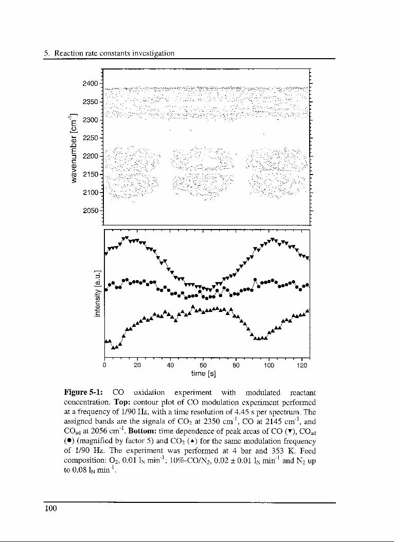
5. Reaction rate constants investigation
1'i 1 1 1 r—i 1—i 1 t
"
] r i i | i i —t- [ i 1 1 j
iEL
"to
<D-i—•
1 1 1 | 1 1 1 | 1 1 1 | 1 7 1 1 1 1 1 1 1 1 1 1—
20 40 60
time [s]
80 100 120
Figure 5-1: CO oxidation experiment with modulated reactant
concentration. Top: contour plot of CO modulation experiment performedat a frequency of 1/90 Hz, with a time resolution of 4.45 s per spectrum. The
assigned bands are the signals of C02 at 2350 cm"1, CO at 2145 cm"1, and
COad at 2056 cm"1. Bottom: time dependence of peak areas of CO (), COaci
(•) (magnified by factor 5) and C02 (a) for the same modulation frequencyof 1/90 Hz. The experiment was performed at 4 bar and 353 K. Feed
composition: 02, 0.01 1N min"1; 10%-CO/N2, 0.02 ± 0.01 1N min"1 and N2 up
to 0.08 1N min"1.
100
5.2 Experimental
The concentration of the feed gas was sinusoidally varied by the desired modulation
frequency and amplitude, ensuring again constant pressure and overall mass flow
conditions. The recording of the spectra was started at the beginning of the modulation
period. Four to five sets of spectra with the same frequency and amplitude were
subsequently collected. Of these sets the first two were always rejected, because they
contained the initial adjustment of the system to the external perturbation.
In Figure 5-1 (top) a contour plot is shown as example for the obtained sets of spectra
(first recorded trace at the left), each trace being recorded within 4.45 seconds. The
phase shift Acp is deduced by plotting the peak area as function of time, the latter
corrected for the measured dead time.
To reduce the error, a mean value was calculated from each measured set of data. In
Figure 5-1 (bottom) an example for the peak area evolution for the CO oxidation is
shown. In the lowest trace (a), the curve does not exhibit the expected sinusoidal
behaviour. In such a case, the phase shift was instead obtained from the maxima and
minima of the time-dependent intensities.
The assigned bands in Figure 5-1 (top) are the signals of: C02 (A) at 2350 cm"1, CO ()
at 2145 cm"1, and COad (•) at 2056 cm"1. The used integration limits are follow: CO2:
2400-2280 cm"1 and 3800-3550 cm"1 for the first overtone; CO: 2270-2075 cm"1; and
COad: 2075-1950 cm"1.
All experiments were performed at a total pressure of 4 bar and at temperatures of 298
K, 326 K, 353 K, 381 K, 408 K, and 436 K. The following feed gas composition were
used to investigate the questions listed below.
1. Interaction of CO with the catalyst: 10%-CO/N2, 0.02 ± 0.011N min"1.
2. Interaction of C02 with the catalyst: C02, 0.05 ± 0.02 1N min"1.
101
5. Reaction rate constants investigation
3. Effect of CO in the CO oxidation reaction: 10%-CO/N2, 0.02 ±0.01 ^min"1; 02,
0.011N min"1.
4. Effect of 02 in the CO oxidation reaction: 02, 0.02 ±0.01 iNmin"1; 10%-CO/N2,
0.04 1N min"1.
Nitrogen was used as carrier and compensation gas. The overall flow was always set to
0.08 1N min"1.
Catalytic reference runs under steady state condition were performed using:
10%-CO/N2, 0.02 1N min"1; 02, 0.01 lNmin"1. After dilution in N2 the gases were
analysed by means of a Siemens IR CO/CO2 analyser (see section 2.7).
5.3 Results and discussion
As explained in chapter 3, the interpretation of the experimental results (phase shifts Acp
or tan[A#?]) of an unknown system as a function of a perturbation (modulation frequency
co) to obtain information about its characteristics is an established method in many
engineering disciplines. A set of differential equation describing the investigated system
is used to obtain the relationships between observed retardation (tan[A#?]) and the data
characterising the considered reaction steps (see section 3.4). From the temperature
dependence, additional thermodynamic parameters of the reactions are determined.
The oxidation of CO can be described by the following microkinetic model: adsorption
of CO, adsorption and dissociation of oxygen, reaction between the two surface species
to form adsorbed C02, and finally, desorption of C02. For each of these steps the
reverse reaction must be considered. The single steps are separately analysed, so that
kinetical data of each step can be estimated. By doing so, it is possible to assess the
validity of the entire microkinetic model.
102
5.3 Results and discussion
5.3.1 Interaction of CO with the catalyst
5.3.1.1 Model
A modulation experiment was carried out to estimate the interaction of CO with the
catalyst surface. Assuming that, for low partial pressures, the surface concentration of
vacant CO adsorption sites is constant, the following simple model can be derived (see
paragraph 3.4.2.1):
h
CO ^=^ coad
Here, k\ and k.\ are effective first order rate constants. As explained in section 3.3.2 the
DRIFT cell can be represented by a continuous stirred tank reactor with residence time
t. With these assumptions the system can be described with the following set of
differential equations:
^o =ÇCjl. {K +I} co + kCO (5>1)
dt T T
dCOad
dt
= k,CO - ^COad (5.2)
where COo represents the CO concentration in the feed gas, CO the concentration of
carbon monoxide in the DRIFT cell, and COad the concentration of the adsorbed species.
Solving the system of differential equations for CO and COad one obtains equations that
are function of co and co2 (see Equation 3.28). As explained in paragraph 3.4.2.1, co2
terms play a role only when high frequencies are applied, it was hence decided to
employ the low frequency approximation. In this way a linearity between tan[A#>] and
the perturbation frequency is obtained:
103
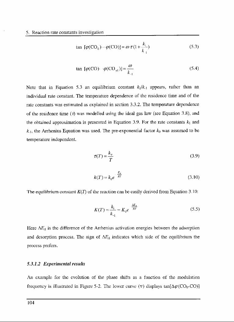
5. Reaction rate constants investigation
tan [(p(CO0)-cp(CO)] = C0T(l + ^-) (5.3)*-i
tan [<p(CO)-^(COad)] =-^- (5.4)
Note that in Equation 5.3 an equilibrium constant k\/L\ appears, rather than an
individual rate constant. The temperature dependence of the residence time and of the
rate constants was estimated as explained in section 3.3.2. The temperature dependence
of the residence time (f) was modelled using the ideal gas law (see Equation 3.8), and
the obtained approximation is presented in Equation 3.9. For the rate constants k\ and
k-\, the Arrhenius Equation was used. The pre-exponential factor ko was assumed to be
temperature independent.
t{T) = ^ (3.9)
-Ea.
k(T) = k0e RT (3.10)
The equilibrium constant K(T) of the reaction can be easily derived from Equation 3.10:
k -^4
K(T) = -^ = K0eRT (5.5)
k-i
Here AEa is the difference of the Arrhenius activation energies between the adsorption
and desorption process. The sign of AEa indicates which side of the equilibrium the
process prefers.
5.3.1.2 Experimental results
An example for the evolution of the phase shifts as a function of the modulation
frequency is illustrated in Figure 5-2. The lower curve (v) displays tan[A«p(COo-CO)]
104
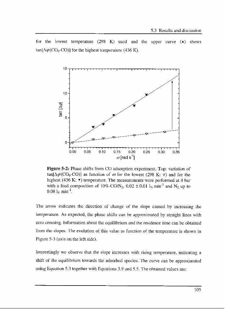
5.3 Results and discussion
for the lowest temperature (298 K) used and the upper curve (±) shows
tan[A#>(CO0-CO)] for the highest temperature (436 K).
15-
10-
c
CO
-i—r—i—r- -i—i—i—i—r-
0.00 0.05 0.10 0.15 0.20 0.25 0.30 0.35
œ [rad s" ]
Figure 5-2: Phase shifts from CO adsorption experiment. Top: variation of
tan[A^(CO0-CO)] as function of co for the lowest (298 K: v) and for the
highest (436 K: ) temperature. The measurements were performed at 4 bar
with a feed composition of 10%-CO/N2, 0.02 ± 0.01 1N min"1 and N2 up to
0.08 1N min"1.
The arrow indicates the direction of change of the slope caused by increasing the
temperature. As expected, the phase shifts can be approximated by straight lines with
zero crossing. Information about the equilibrium and the residence time can be obtained
from the slopes. The evolution of this value as function of the temperature is shown in
Figure 5-3 (axis on the left side).
Interestingly we observe that the slope increases with rising temperature, indicating a
shift of the equilibrium towards the adsorbed species. The curve can be approximated
using Equation 5.3 together with Equations 3.9 and 5.5. The obtained values are:
105
5. Reaction rate constants investigation
40-
r-,35-1
oO 30O
oO 25^
^20^c
CO
S.KH_oW
5^
0-
40
:35
j-30
-25
P20^v
15
|-10
i-5
-0
—I ' 1 ' 1 ' 1 ' 1 ' 1 ' 1 '
0.0022 0.0024 0.0026 0.0028 0.0030 0.0032 0.0034
temperature"1 [K~1]
Figure 5-3: Left: Variation of the slopes for tan[A^(CO0-CO)] () as
function of temperature. The curve was modelled using Equation 5.3, with
Equations 3.9 and 5.5. Right: Arrhenius plot for the variation of the slopesof tan[A#>(CO-COad)] (•) with the temperature. The curve was modelled
using Equations 5.4 and 3.10. Experimental conditions as in Figure 5-2.
fcc = l'331±267Ks ü:oi = 8'841±2'018 AEA1=24.1±1.4kJmol"1
The equilibrium is characterised by Kq,i and A£a,i, and the geometry of the reactor by kz.
AEa,i is positive indicating that the adsorption reaction is energy consuming. This result
agrees with the observation that COad exists spectroscopically only in the presence of
gas phase CO (data not shown).
The phase shift evolution between CO and COad provides information about the reverse
reaction. The slopes obtained from the phase shifts decrease with increasing
temperature. This indicates an enhanced desorption at higher temperatures. For an
Arrhenius plot, Equation 3.10 was inserted into Equation 5.4 and solved for ln(&_i). The
experimental data for the slopes of tan[A^(CO-COad)] were analysed according to this
106
5.3 Results and discussion
new equation. The temperature dependence of ln(fc.i) is shown in Figure 5-3 (axis on the
right side), from which Ea-\ and fco,-i are simply estimated. The obtained values are:
*b,.i = 1.95-108 ± 1.81-108 s"1 Eaa = 46.1 ± 2.6 kJ mol"1
In Figure 5-3, only the four lowest temperatures are plotted, because at high
temperatures the amplitude of the variation of the concentration was not large enough to
define the phase shift within an acceptable error. Even for the used values the error is
already quite high for kor\.
Approximated values for the Arrhenius energy and pre-exponential factor of the
adsorption reaction, Ea,i and £o,i respectively, can be derived from the numbers given
above:
Jfeo,i = 1.72-1012 ± 1.64-1012 s"1 EA,i = 70.2 ± 3.0 kJ mol"1
The obtained pre-exponential factor shows a relatively high error due to the uncertainty
of &o,-i. These apparent standard deviations of the pre-exponential values (fco.i, &o,-i) can
be traced back to the assumption that ko is temperature independent. The obtained
values should serve only as a hint for the adsorption/desorption reaction rates.
As a reference it is noteworthy that the activation energy for the desorption (E^des) of
singly bound CO on pure Pd was estimated to be 56.4 kJ mol"1 [146].
5.3.2 Interaction of CO2 with the catalyst
5.3.2.1 Model
As described above for CO, also in this experiment the interaction of a reactant gas
(C02) with the catalyst surface was investigated (see paragraph 3.4.2.1). Under the used
conditions no adsorbed C02 (C02,ad), neither reaction products like COad nor
107
5. Reaction rate constants investigation
carbonates, were observed. However this does not exclude the existence of these species
on the surface at a concentration below the detection limit of DRIFT. Therefore, it is not
possible to exclude that, applying different reaction conditions, C02 could be adsorbed
and dissociated, e. g., into COad and adsorbed oxygen (Oad). Hints about a similar
reaction were already found by Nijhuis et al. [154] for C02 adsorption on Pt using a
TAP reactor system.
The used model considers that a possible adsorption/desorption reaction can take place.
Like in the case of CO, it was assumed that, during the experiment, the surface
concentration of vacant C02 adsorption sites is constant. The simplified model can be
written as:
co2 ^^ co2,adk-3
Like above, the same presumptions are valid in this case: a) k3 and fc.3 are effective first
order rate constants, and b) the DRIFT cell can be represented by a continuous stirred
tank reactor with residence time T. With these assumptions, we can describe the system
only by using Equation 5.1, where, however, CO should be substituted with C02, k\
with k3 and k.\ with k.3. Equation 5.2 can not be applied, because a matching surface
species was not observed. With the same considerations as in the previous section for
CO, we can write:
tan [Aç{CO20-CO2)] = cot(1 + -^-) (5.6)
where C02o represents the gas phase concentration of carbon dioxide in the feed gas
and C02 in the DRIFT cell. Also like in Equation 5.3, Equation 5.6 approximates an
equilibrium constant. The evolution of t is approximated with Equation 3.9 and the
equilibrium constant with Equation 5.5.
108
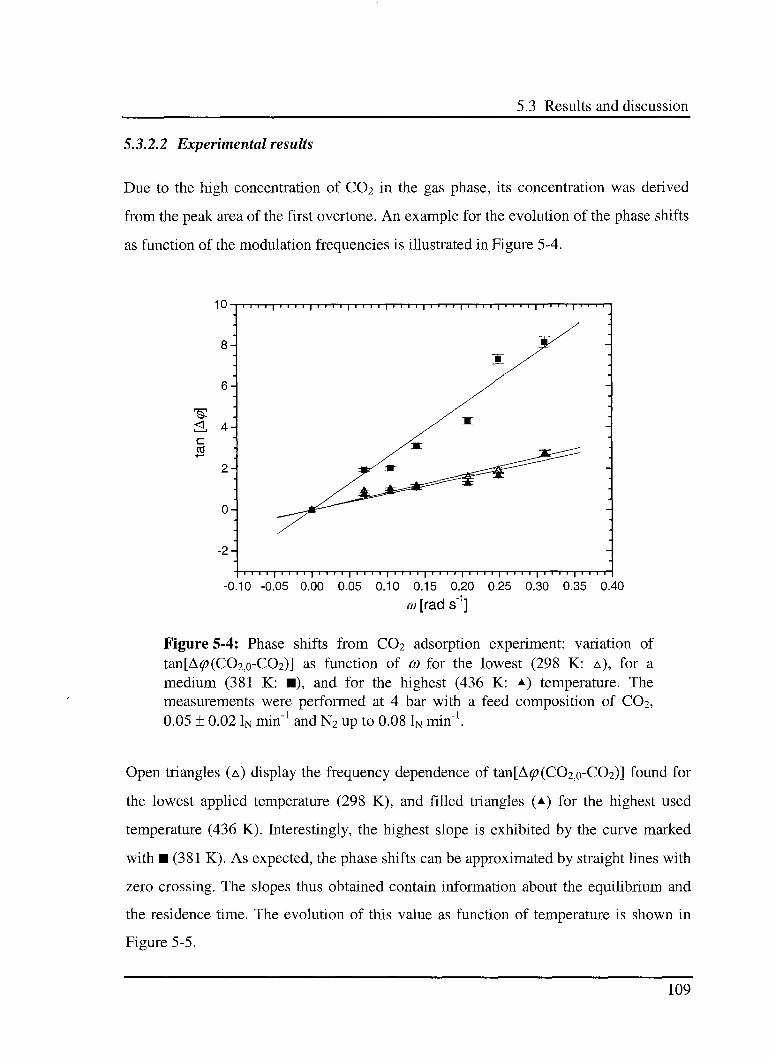
5.3 Results and discussion
5.3.2.2 Experimental results
Due to the high concentration of C02 in the gas phase, its concentration was derived
from the peak area of the first overtone. An example for the evolution of the phase shifts
as function of the modulation frequencies is illustrated in Figure 5-4.
10-
8-
6-
< 4-|c
CO
0-
-2-
1 ' ' i ' ' I ' ' i ' ' ' I i i i i i i i i i i i i i i i i i ii i i
i i i i i i i i i i i i i l i i i i i i i i i i i i i i i i i i i i i i i i l i i i i i i i i
-0.10 -0.05 0.00 0.05 0.10 0.15 0.20 0.25 0.30 0.35 0.40
co [rad s1]
Figure 5-4: Phase shifts from C02 adsorption experiment: variation of
tan[A^(CO2j0-CO2)] as function of co for the lowest (298 K: a), for a
medium (381 K: ), and for the highest (436 K: ±) temperature. The
measurements were performed at 4 bar with a feed composition of C02,
0.05 ± 0.02 1N min"1 and N2 up to 0.08 1N min"1.
Open triangles (a) display the frequency dependence of tan[A<p(CO2j0-CO2)] found for
the lowest applied temperature (298 K), and filled triangles (a) for the highest used
temperature (436 K). Interestingly, the highest slope is exhibited by the curve marked
with (381 K). As expected, the phase shifts can be approximated by straight lines with
zero crossing. The slopes thus obtained contain information about the equilibrium and
the residence time. The evolution of this value as function of temperature is shown in
Figure 5-5.
109
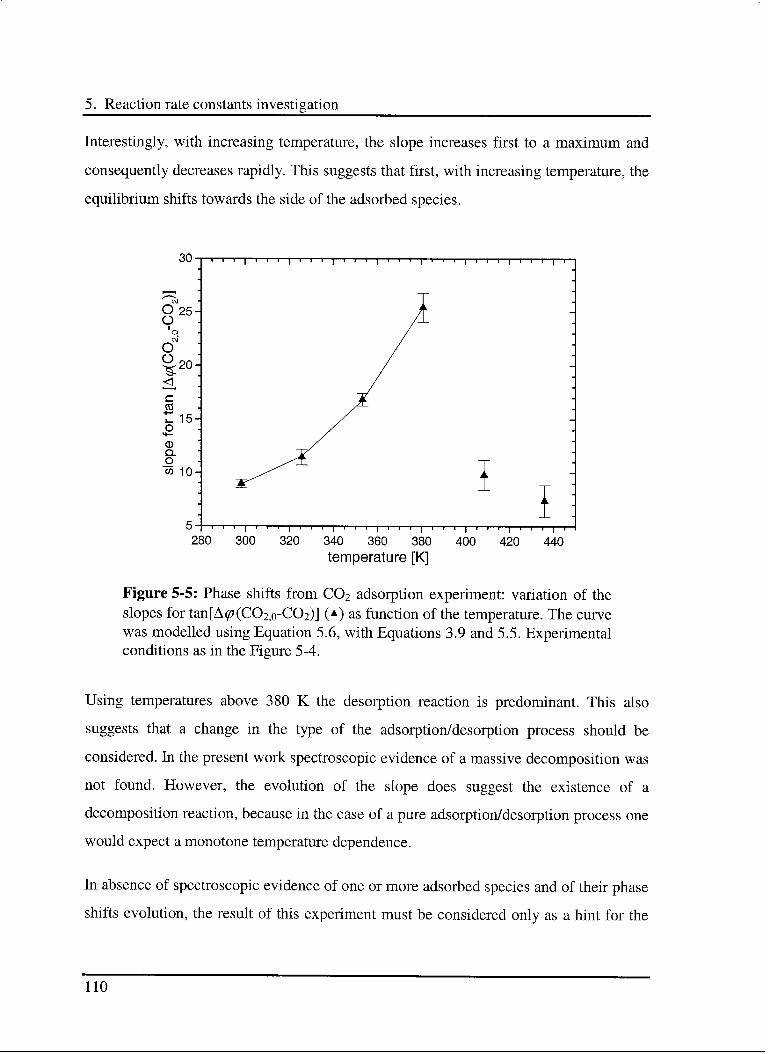
5. Reaction rate constants investigation
Interestingly, with increasing temperature, the slope increases first to a maximum and
consequently decreases rapidly. This suggests that first, with increasing temperature, the
equilibrium shifts towards the side of the adsorbed species.
30 -1—l—l—l—|—i—i—l—|—l—l—l—|—l—i—l—|—l—l—l—|—l—i—l—|—l—l—l—J—l—l—l—|—r
CM
825:o
cm"
o
;<L -
c
CO
r 15-oM—
0Q.
O
W 10-
5 I i i i i i i i | i i i i i i i | i i i | i i i | i i i | i i i | i
280 300 320 340 360 380 400 420 440
temperature [K]
Figure 5-5: Phase shifts from C02 adsorption experiment: variation of the
slopes for tan[A#?(CO2i0-CO2)] (a) as function of the temperature. The curve
was modelled using Equation 5.6, with Equations 3.9 and 5.5. Experimentalconditions as in the Figure 5-4.
Using temperatures above 380 K the desorption reaction is predominant. This also
suggests that a change in the type of the adsorption/desorption process should be
considered. In the present work spectroscopic evidence of a massive decomposition was
not found. However, the evolution of the slope does suggest the existence of a
decomposition reaction, because in the case of a pure adsorption/desorption process one
would expect a monotone temperature dependence.
In absence of spectroscopic evidence of one or more adsorbed species and of their phase
shifts evolution, the result of this experiment must be considered only as a hint for the
?
110
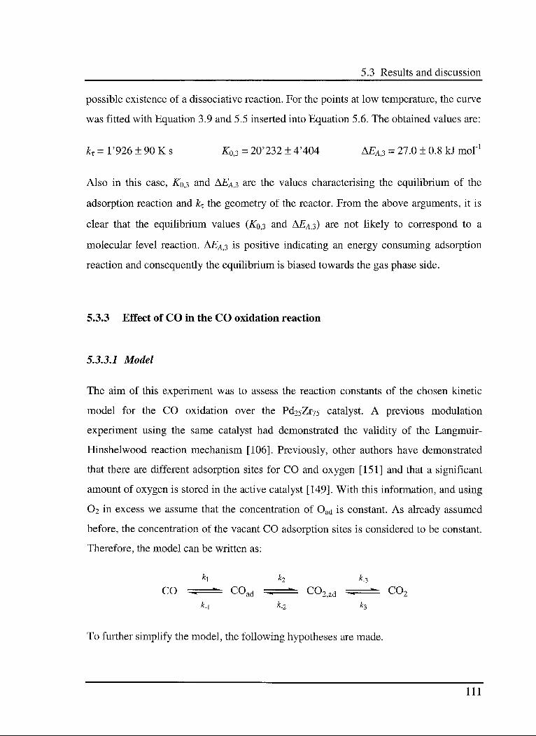
5.3 Results and discussion
possible existence of a dissociative reaction. For the points at low temperature, the curve
was fitted with Equation 3.9 and 5.5 inserted into Equation 5.6. The obtained values are:
Jkt=l'926±90Ks £0,3 = 20'232 ±4'404 AEA,3 = 27.0 ± 0.8 kJ mol"1
Also in this case, £0,3 and A£a,3 are the values characterising the equilibrium of the
adsorption reaction and k^ the geometry of the reactor. From the above arguments, it is
clear that the equilibrium values (K0j and AEA,s) are not likely to correspond to a
molecular level reaction. A£a,3 is positive indicating an energy consuming adsorption
reaction and consequently the equilibrium is biased towards the gas phase side.
5.3.3 Effect of CO in the CO oxidation reaction
5.3.3.1 Model
The aim of this experiment was to assess the reaction constants of the chosen kinetic
model for the CO oxidation over the Pd25Zr75 catalyst. A previous modulation
experiment using the same catalyst had demonstrated the validity of the Langmuir-
Hinshelwood reaction mechanism [106]. Previously, other authors have demonstrated
that there are different adsorption sites for CO and oxygen [151] and that a significant
amount of oxygen is stored in the active catalyst [149]. With this information, and using
02 in excess we assume that the concentration of Oad is constant. As already assumed
before, the concentration of the vacant CO adsorption sites is considered to be constant.
Therefore, the model can be written as:
CO ^=^ coad ^=^ co2,ad ^=^ co2
k_i k_2 fc3
To further simplify the model, the following hypotheses are made.
Ill
5 Reaction rate constants investigation
(1) Excess of oxygen allows to assume a saturation of Oad on the surface As a
consequence the rate constant of the COad oxidation process is faster than its back
reaction (k2 » k2).
(2) As discussed in paragraph 5 3 2 2, the positive value of AEa 3 suggests that the
equilibrium of the C02 adsorption is shifted to the side of the gas phase Therefore, we
can assume a very small C02 adsorption rate as compared to the desorption rate
(k3»k3)
(3) As a further consequence, the desorption rate of CO2 ad should be much faster than
the oxidation rate of COad {k 3 » k2)
The two steps from COad to gaseous C02 may hence be combined into one, and the four
reactions (characterised by constants k2, k2,k3 and £3) are replaced by a single one-side
reaction, with rate constant k2 This simplification appears adequate m view of the fact
that C02 ad was not observed spectroscopically
(4) Assuming that a single reaction step is rate limiting, the constants k\ and k 1 of the
CO adsorption/desorption process can be replaced with a net reaction constant k{ This
constant describes the overall process as COad production If the CO adsorption step is
rate limiting, k{ represents a rate constant If the COad oxidation is rate limiting, k{
measures the net production rate of COad from gaseous CO
Thus the following simple model was obtained
k{ kj
CO coad co2
Additional information about similar system can be found in paragraph 3 4 2 2 Here k\'
and k2 are effective first order rate constants The DRIFT cell is again represented as a
continuous stirred tank reactor Consequently, we can describe this system by the
following set of differential equations
112
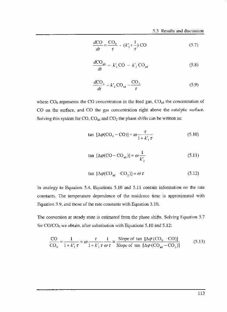
5.3 Results and discussion
ÉÇ9.=99sl
. (k\+~) co (5.7)dt T T
dCO
j
= k\CO -k\ COad (5.8)dt
dCO,,, _
CO,
dt2-fe'2COad
*- (5.9)
where CO0 represents the CO concentration in the feed gas, COad the concentration of
CO on the surface, and CO the gas concentration right above the catalytic surface.
Solving this system for CO, COad and C02 the phase shifts can be written as:
tan [A^(CO0 - CO)] = co—T-T- (5.10)1t/Ci T
tan [A^(CO-COad)] = w^- (5.11)k
2
tan [A^(COad -C02)] = cot (5.12)
In analogy to Equation 5.4, Equations 5.10 and 5.11 contain information on the rate
constants. The temperature dependence of the residence time is approximated with
Equation 3.9, and those of the rate constants with Equation 3.10.
The conversion at steady state is estimated from the phase shifts. Solving Equation 5.7
for CO/COo we obtain, after substitution with Equations 5.10 and 5.12:
CO 1 T \ Slope of tan [Acp (COn - CO)]= co =
—t—: Q— (5.13)
CO0 l + k\T l + k\TCOT Slope of tan [A<p(COad-C02)]
113
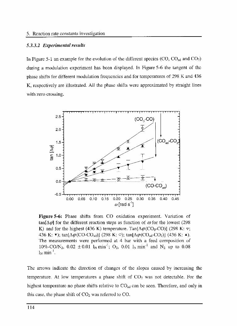
5. Reaction rate constants investigation
5.3.3.2 Experimental results
In Figure 5-1 an example for the evolution of the different species (CO, COad and C02)
during a modulation experiment has been displayed. In Figure 5-6 the tangent of the
phase shifts for different modulation frequencies and for temperatures of 298 K and 436
K, respectively are illustrated. All the phase shifts were approximated by straight lines
with zero crossing.
-0.5
(coad-coj
(CO-COJ
I I I I I I I I I I I I I I I I I » I I I I I I I I I I I I I I I
0.00 0.05 0.10 0.15 0.20 0.25 0.30 0.35 0.40 0.45
œ [rad s~1]
Figure 5-6: Phase shifts from CO oxidation experiment. Variation of
tan[A^] for the different reaction steps as function of co for the lowest (298
K) and for the highest (436 K) temperature. Tan[A<p(CO0-CO)] (298 K: v;
436 K: ); tan[A^(CO-COad)] (298 K: o); tan[A<p(COad-C02)] (436 K: a).The measurements were performed at 4 bar with a feed composition of
10%-CO/N2, 0.02 ±0.01 1N min"1; 02, 0.01 lNimn"1 and N2 up to 0.08
In min".
The arrows indicate the direction of changes of the slopes caused by increasing the
temperature. At low temperatures a phase shift of C02 was not detectable. For the
highest temperature no phase shifts relative to COad can be seen. Therefore, and only in
this case, the phase shift of CO2 was referred to CO.
114
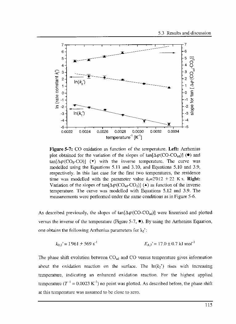
5.3 Results and discussion
c
CO
toc
oÜ
Q)+->
CO
0.0022 0.0024 0.0026 0.0028 0.0030
temperature"1 [K"1]
i r
0.0032 0.0034
Figure 5-7: CO oxidation as function of the temperature. Left: Arrhenius
plot obtained for the variation of the slopes of tan[A^(CO-COad)] (•) and
tan[A#>(CO0-CO)] () with the inverse temperature. The curve was
modelled using the Equations 5.11 and 3.10, and Equations 5.10 and 3.9,
respectively. In this last case for the first two temperatures, the residence
time was modelled with the parameter value kx-2X)l2 ±22 K s. Right:
Variation of the slopes of tan[A^(COad-C02)] (a) as function of the inverse
temperature. The curve was modelled with Equations 5.12 and 3.9. The
measurements were performed under the same conditions as in Figure 5-6.
As described previously, the slopes of tan[A<p(CO-COad)] were linearised and plotted
versus the inverse of the temperature (Figure 5-7, •). By using the Arrhenius Equation,
one obtains the following Arrhenius parameters for k2' :
£0,2'= 1961 ± 569 s"1-A,2 17.0 ± 0.7 kJ mol"1
The phase shift evolution between COad and CO versus temperature gives information
about the oxidation reaction on the surface. The ln(£2') rises with increasing
temperature, indicating an enhanced oxidation reaction. For the highest applied
temperature (T1 = 0.0023 K'1) no point was plotted. As described before, the phase shift
at this temperature was assumed to be close to zero.
115
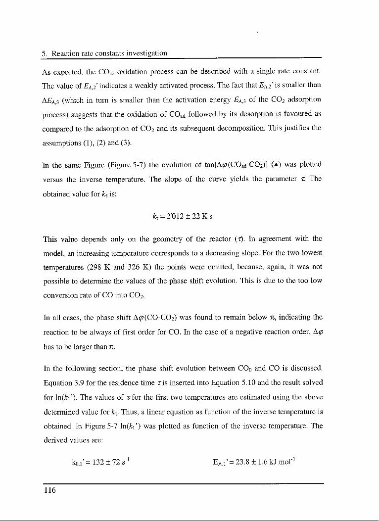
5. Reaction rate constants investigation
As expected, the COad oxidation process can be described with a single rate constant.
The value of Ea,2 indicates a weakly activated process. The fact that Ea,2 is smaller than
A£a,3 (which in turn is smaller than the activation energy £a,3 of the C02 adsorption
process) suggests that the oxidation of COad followed by its desorption is favoured as
compared to the adsorption of C02 and its subsequent decomposition. This justifies the
assumptions (1), (2) and (3).
In the same Figure (Figure 5-7) the evolution of tan[A#?(COad-C02)] (a) was plotted
versus the inverse temperature. The slope of the curve yields the parameter r. The
obtained value for kx is:
fet = 2X)12 ± 22 K s
This value depends only on the geometry of the reactor (t). In agreement with the
model, an increasing temperature corresponds to a decreasing slope. For the two lowest
temperatures (298 K and 326 K) the points were omitted, because, again, it was not
possible to determine the values of the phase shift evolution. This is due to the too low
conversion rate of CO into C02.
In all cases, the phase shift A^(CO-C02) was found to remain below n, indicating the
reaction to be always of first order for CO. In the case of a negative reaction order, Acp
has to be larger than n.
In the following section, the phase shift evolution between COo and CO is discussed.
Equation 3.9 for the residence time ris inserted into Equation 5.10 and the result solved
for ln(fci'). The values of rfor the first two temperatures are estimated using the above
determined value for k^. Thus, a linear equation as function of the inverse temperature is
obtained. In Figure 5-7 ln(k\') was plotted as function of the inverse temperature. The
derived values are:
ko,i'= 132 ± 72 s"1 EA,i'= 23.8 ± 1.6 kJ mol"1
116
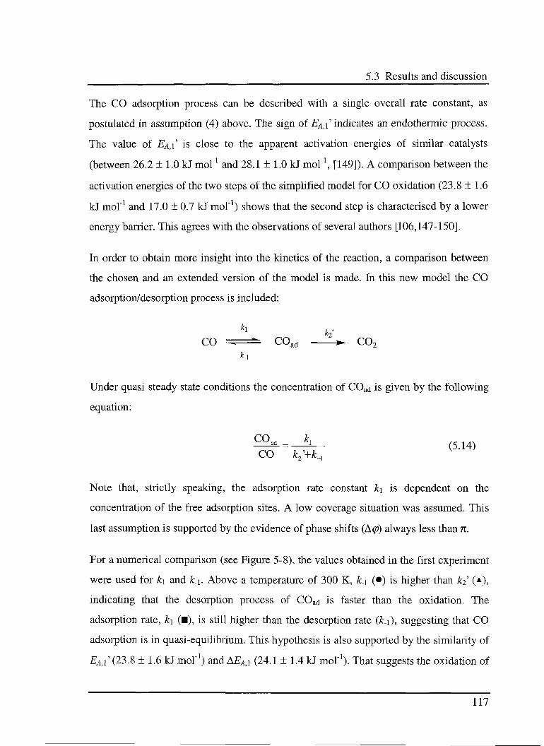
5.3 Results and discussion
The CO adsorption process can be described with a single overall rate constant, as
postulated in assumption (4) above. The sign of EA,\ indicates an endothermic process.
The value of Ea,\ is close to the apparent activation energies of similar catalysts
(between 26.2 ± 1.0 kJ mol"1 and 28.1 ± 1.0 kJ mol"1, [149]). A comparison between the
activation energies of the two steps of the simplified model for CO oxidation (23.8 ±1.6
kJ mol"1 and 17.0 ± 0.7 kJ mol"1) shows that the second step is characterised by a lower
energy barrier. This agrees with the observations of several authors [106,147-150].
In order to obtain more insight into the kinetics of the reaction, a comparison between
the chosen and an extended version of the model is made. In this new model the CO
adsorption/desorption process is included:
CO .
*
coad co2
Under quasi steady state conditions the concentration of COad is given by the following
equation:
^L=—*L_
(5.14)CO k2+k_x
Note that, strictly speaking, the adsorption rate constant k\ is dependent on the
concentration of the free adsorption sites. A low coverage situation was assumed. This
last assumption is supported by the evidence of phase shifts {Acp) always less than n.
For a numerical comparison (see Figure 5-8), the values obtained in the first experiment
were used for k\ and k.\. Above a temperature of 300 K, k_i (•) is higher than k2 (a),
indicating that the desorption process of COad is faster than the oxidation. The
adsorption rate, k\ (), is still higher than the desorption rate (k.\), suggesting that CO
adsorption is in quasi-equilibrium. This hypothesis is also supported by the similarity of
EAy (23.8 ± 1.6 kJ mol"1) and AEAA (24.1 ± 1.4 kJ mol"1). That suggests the oxidation of
117
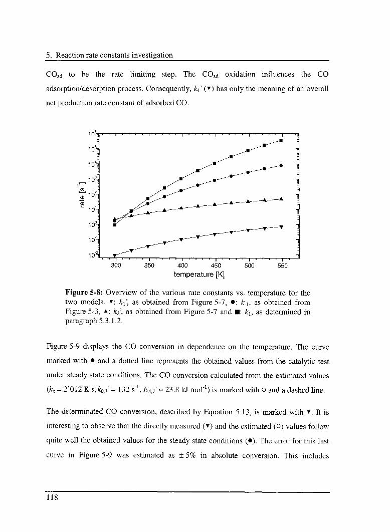
5. Reaction rate constants investigation
COad to be the rate limiting step. The COad oxidation influences the CO
adsorption/desorption process. Consequently, k\' () has only the meaning of an overall
net production rate constant of adsorbed CO.
10V1—'—i-1—'—'—'—1—r—1—'—"""i—'—I—'—'—1—'—'—'—'—r-1—'—'—l—i—I—1
300 350 400 450 500 550
temperature [K]
Figure 5-8: Overview of the various rate constants vs. temperature for the
two models. : k\, as obtained from Figure 5-7, •: k.\, as obtained from
Figure 5-3, a; k2\ as obtained from Figure 5-7 and : k\, as determined in
paragraph 5.3.1.2.
Figure 5-9 displays the CO conversion in dependence on the temperature. The curve
marked with • and a dotted line represents the obtained values from the catalytic test
under steady state conditions. The CO conversion calculated from the estimated values
(fct = 2'012 K s,£0,i' = 132 s"1, EA,\ = 23.8 kJ mol"1) is marked with o and a dashed line.
The determinated CO conversion, described by Equation 5.13, is marked with . It is
interesting to observe that the directly measured () and the estimated (o) values follow
quite well the obtained values for the steady state conditions (•). The error for this last
curve in Figure 5-9 was estimated as ± 5% in absolute conversion. This includes
118
5.3 Results and discussion
possible unstabilities (e. g. oscillations and deviations) of the steady state equilibria and
instrumentation. One can easily see that the applied model agrees well with the reality.
0.8-r
07-
06-
O 05-w
5 04-c
o
»0.3-
Ü
02-
01-
00-
-I I I | "1 I I 1 | -i—I—i—i—i—I—i—i—I I I—r
C)
<r -L
l"i"
r t | i i—i—i—| i i i i |—i i i i—p
250 300 350 400 450 500
temperature [K]550 600
Figure 5-9: Comparison of experimental and measured CO conversions. :
CO conversion estimated from the slopes of the phase shifts, as given by
Equation 5.13. o and dashed line: CO conversion calculated from the
estimated values, hl = T0\2 Ks, k0= 132 s \ EA,i=23.S kJmol1. • and
dotted line: CO conversion measured under steady state conditions, no
modulation, experimental error ± 0.05. The measurements under steady state
conditions were performed at 4 bar with a feed composition of 10%-CO/N2,
0.02 1N nun 1; 02, 0 011N mm"1 and N2 up to 0.08 1N mm l.
5.3.4 Effect of 02 in the CO oxidation reaction
5.3.4.1 Model
Finally, the influence of 02 onto the oxidation reaction should be estimated. In analogy
to the previous experiments (see section 5 3.3), CO was used in excess, and therefore
the concentration of adsorbed carbon monoxide (COad) was assumed to be constant.
119
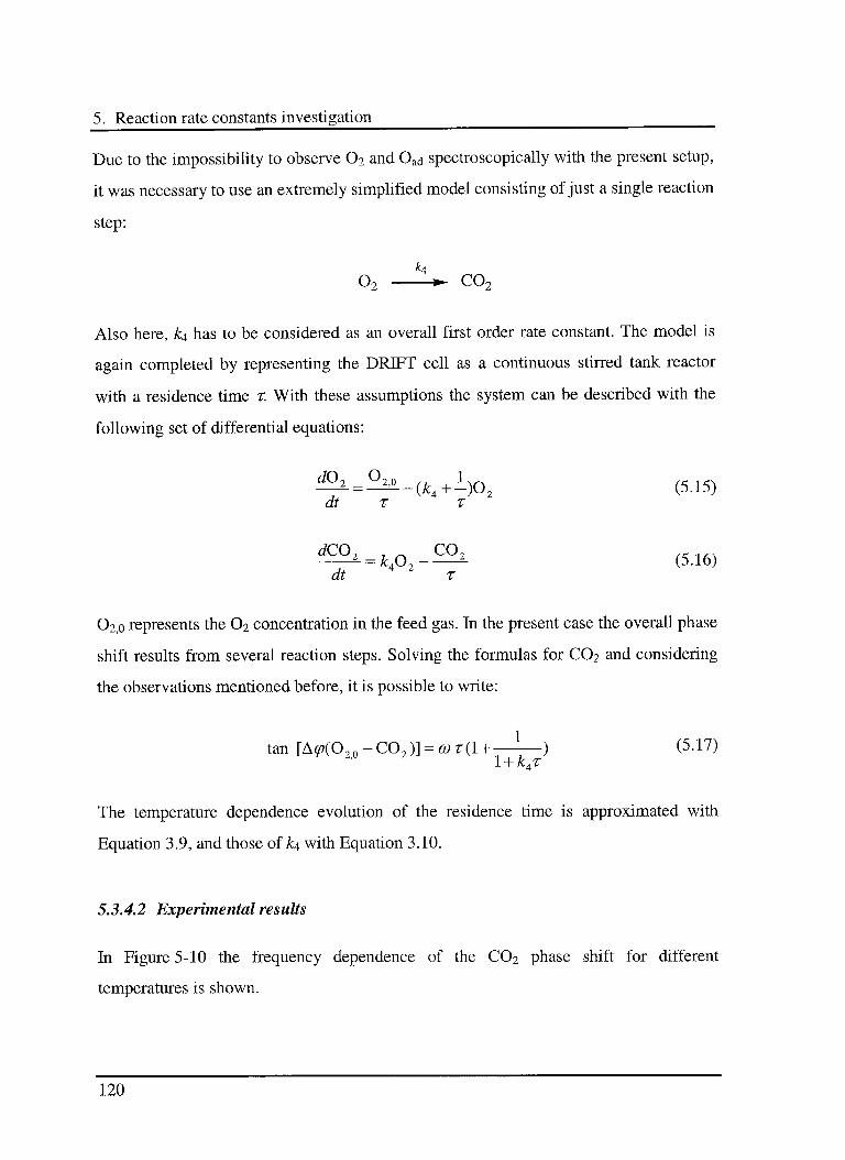
5. Reaction rate constants investigation
Due to the impossibility to observe 02 and Oad spectroscopically with the present setup,
it was necessary to use an extremely simplified model consisting of just a single reaction
step:
o2 co2
Also here, £4 has to be considered as an overall first order rate constant. The model is
again completed by representing the DRIFT cell as a continuous stirred tank reactor
with a residence time r. With these assumptions the system can be described with the
following set of differential equations:
^ = ^-(£4+I)02 (5.15)dt T T
dt
02ß represents the O2 concentration in the feed gas. In the present case the overall phase
shift results from several reaction steps. Solving the formulas for C02 and considering
the observations mentioned before, it is possible to write:
tan [A<p(O20-CO2)] = ft>r(l +—-—) (5.17)l + k4T
The temperature dependence evolution of the residence time is approximated with
Equation 3.9, and those of ki, with Equation 3.10.
5.3.4.2 Experimental results
In Figure 5-10 the frequency dependence of the C02 phase shift for different
temperatures is shown.
120
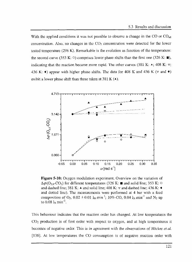
5.3 Results and discussion
With the applied conditions it was not possible to observe a change in the CO or COad
concentration. Also, no changes in the C02 concentration were detected for the lower
tested temperature (298 K). Remarkable is the evolution as function of the temperature:
the second curve (353 K: o) comprises lower phase shifts than the first one (326 K: ),
indicating that the reaction became more rapid. The other curves (381 K: a; 408 K: v;
436 K: ) appear with higher phase shifts. The data for 408 K and 436 K (v and )
exibit a lower phase shift than these taken at 381 K (a).
4.713-
3.142-
OÜ
<
1.571-
0.000
I I 1—I—p -I—I—I—I—|—I—I—I—I—|—I—I—I—I—f**|—I—I—I—J"
$----g
-0.05 0.00 0.05 0.10 0.15 0.20 0.25 0.30 0.35
co [rad s"1]
Figure 5-10: Oxygen modulation experiment. Overview on the variation of
A^(02,o-C02) for different temperatures (326 K: and solid line; 353 K: o
and dashed line; 381 K: a and solid line; 408 K: v and dashed line; 436 K:
and dotted line). The measurements were performed at 4 bar with a feed
composition of 02, 0.02 ± 0.01 lNimn"1; 10%-CO, 0.04 lNmin"1 and N2 up
to 0.08 1N min"1.
This behaviour indicates that the reaction order has changed. At low temperatures the
C02 production is of first order with respect to oxygen, and at high temperatures it
becomes of negative order. This is in agreement with the observations of Böcker et al.
[136]. At low temperatures the CO consumption is of negative reaction order with
121
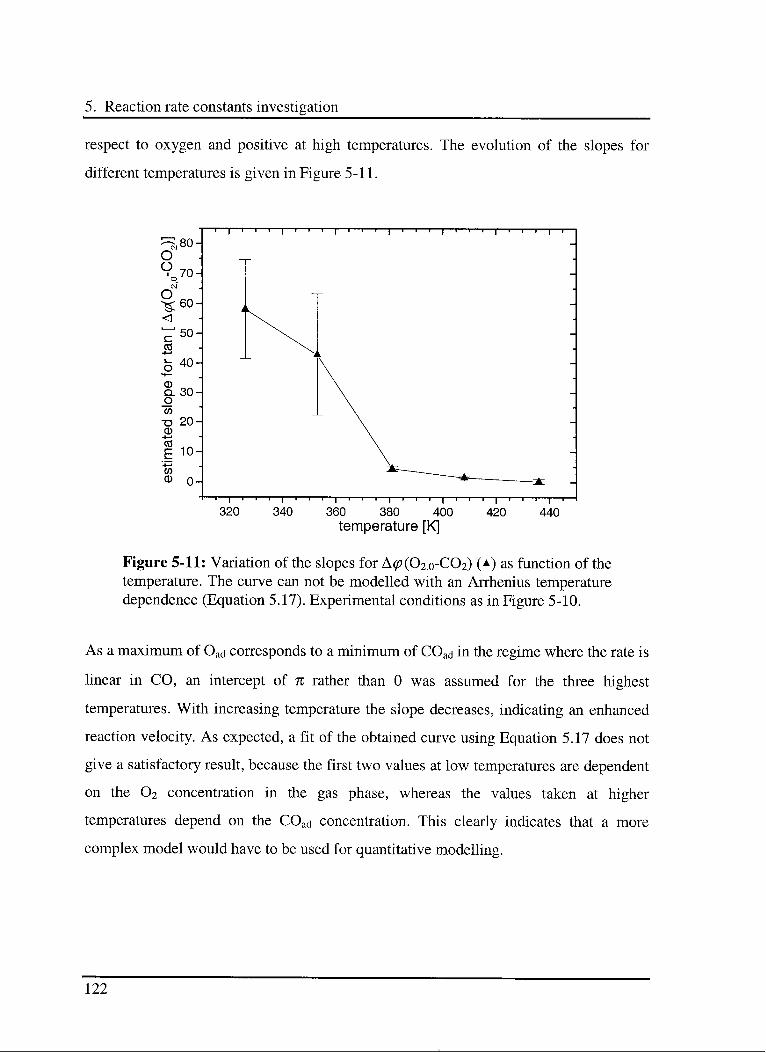
5. Reaction rate constants investigation
respect to oxygen and positive at high temperatures. The evolution of the slopes for
different temperatures is given in Figure 5-11.
^80-O
—i—|—i—i—i—|—i—i—i—|—i—i—i—|—i—i—i—|—p—i—i—|—i—i—i—|—i—
9o70-o
cm".
o^60- -
<
-50- -
c0 .
+-• \ k
o4°- \
*+— \
CDa. 30- \o
w>
-a 20- \
cd+-"
tö_„
g 10- \
CD 0-3fe—__________^
:Ai
i i i i i i i i i i i i i i i i i i i i i i i i i
320 340 360 380 400 420 440
temperature [K]
Figure 5-11: Variation of the slopes for A#>(02,o-C02) (A) as function of the
temperature. The curve can not be modelled with an Arrhenius temperature
dependence (Equation 5.17). Experimental conditions as in Figure 5-10.
As a maximum of Oad corresponds to a minimum of COad in the regime where the rate is
linear in CO, an intercept of n rather than 0 was assumed for the three highest
temperatures. With increasing temperature the slope decreases, indicating an enhanced
reaction velocity. As expected, a fit of the obtained curve using Equation 5.17 does not
give a satisfactory result, because the first two values at low temperatures are dependent
on the 02 concentration in the gas phase, whereas the values taken at higher
temperatures depend on the COad concentration. This clearly indicates that a more
complex model would have to be used for quantitative modelling.
122
5.4 Error sources
5.4 Error sources
In this paragraph possible sources of errors and their influence on the results are
discussed.
5.4.1 Signal-to-Noise Ratio (SNR)
An important error source is certainly the low Signal-to-Noise Ratio (SNR). As
explained in section 3.3.4, if the SNR is not good enough, the measured signal can
contain artefacts. After defining the measurement conditions (aperture, scan velocity,
filter, etc.), the SNR is dependent on the number of collected scans per spectrum, the
concentration of the different species, and the IR emissivity of the sample.
In our case, the number of photons is low (ca. 250 photons per second). This effect is
due to the greyish-black colour of the catalyst, exhibiting a strong absorption in the
mid-IR region. For each spectrum several interferograms were accumulated, but the
collection time is limited by the time resolution required to resolve the phase during a
modulation cycle.
5.4.2 Phase resolution
Six points per period were collected for several modulation periods, at any given
modulation frequency, to reduce the error caused by the approximation of the sinusoidal
curve. With this data set, it was possible to approximate the obtained points with a
sinusoidal function over several periods.
123
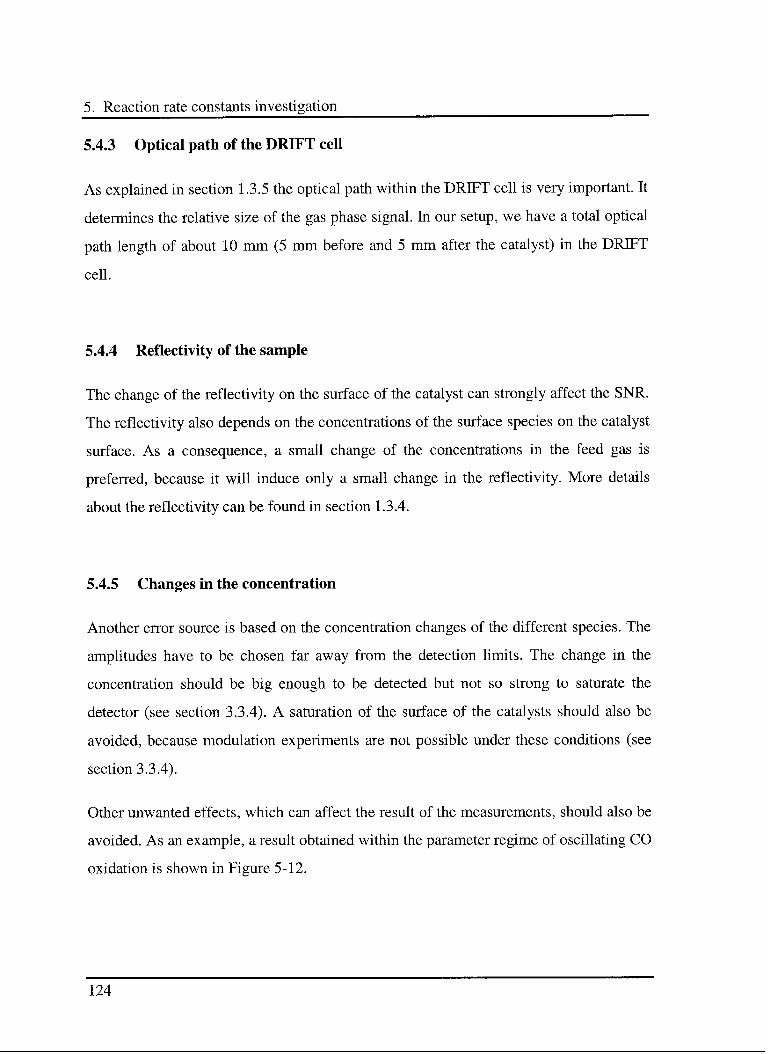
5. Reaction rate constants investigation
5.4.3 Optical path of the DRIFT cell
As explained in section 1.3.5 the optical path within the DRIFT cell is very important. It
determines the relative size of the gas phase signal. In our setup, we have a total optical
path length of about 10 mm (5 mm before and 5 mm after the catalyst) in the DRIFT
cell.
5.4.4 Reflectivity of the sample
The change of the reflectivity on the surface of the catalyst can strongly affect the SNR.
The reflectivity also depends on the concentrations of the surface species on the catalyst
surface. As a consequence, a small change of the concentrations in the feed gas is
preferred, because it will induce only a small change in the reflectivity. More details
about the reflectivity can be found in section 1.3.4.
5.4.5 Changes in the concentration
Another error source is based on the concentration changes of the different species. The
amplitudes have to be chosen far away from the detection limits. The change in the
concentration should be big enough to be detected but not so strong to saturate the
detector (see section 3.3.4). A saturation of the surface of the catalysts should also be
avoided, because modulation experiments are not possible under these conditions (see
section 3.3.4).
Other unwanted effects, which can affect the result of the measurements, should also be
avoided. As an example, a result obtained within the parameter regime of oscillating CO
oxidation is shown in Figure 5-12.
124
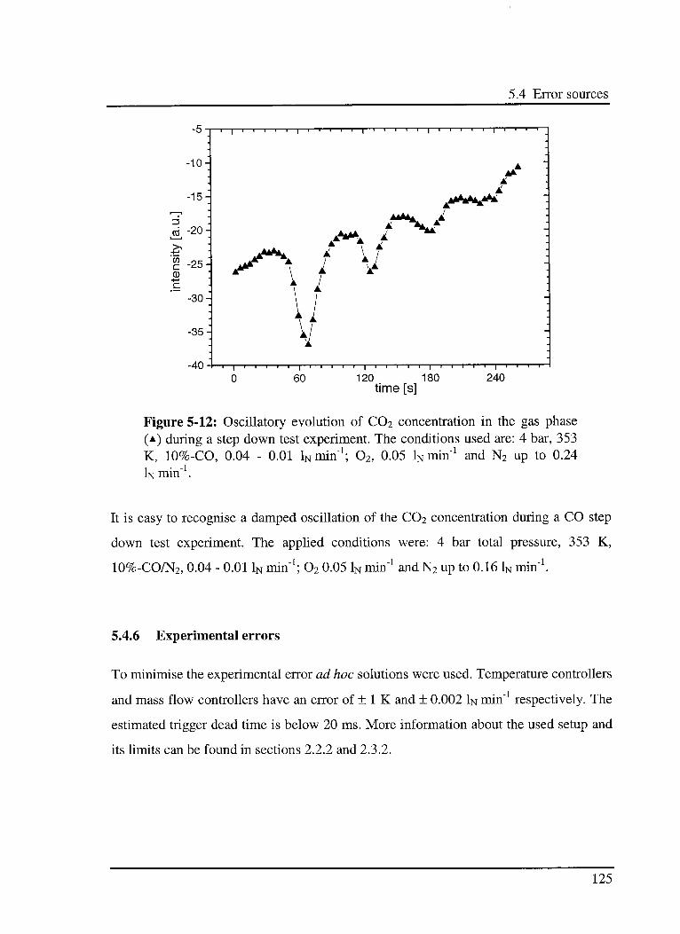
5.4 Error sources
-10-
-15-
cd -20 H
g -25 HCD
-30-
-35-
-40
-|—i—r—i—i—i—|—r—i—i i i—|—i—r—i—i—i—p -i—i—i i
^AAAjAè^Aà
S/
^/ w
wH
' I ' -i—r—i—i—i —r~ i |—i—r—i—r"
60 120 180
time [s]240
Figure 5-12: Oscillatory evolution of C02 concentration in the gas phase
(a) during a step down test experiment. The conditions used are: 4 bar, 353
K, 10%-CO, 0.04 - 0.01 lNmin"1; 02, 0.05 iNmin"1 and N2 up to 0.24
In min".
It is easy to recognise a damped oscillation of the C02 concentration during a CO step
down test experiment. The applied conditions were: 4 bar total pressure, 353 K,
10%-CO/N2, 0.04 - 0.011N min"1; 02 0.05 1N min"1 and N2 up to 0.16 1N min"1.
5.4.6 Experimental errors
To minimise the experimental error ad hoc solutions were used. Temperature controllers
and mass flow controllers have an error of ± 1 K and ± 0.002 1N min"1 respectively. The
estimated trigger dead time is below 20 ms. More information about the used setup and
its limits can be found in sections 2.2.2 and 2.3.2.
125
5. Reaction rate constants investigation
5.4.7 Dead time
The dead time estimation is important to define the start of a modulation period and
consequently the phase shift Acp between the species (see paragraph 3.3.4.1). The dead
time monitored during the different experiments at different temperatures is shown in
Figure 5-13.
ou- i i i i i i i i i i i i i i i I i "T 1 1 1 T'
| l l l | i i i 1 i
25- -
"w1
0 20-
* =*= Ï==
I
i
i
1
M
.1-t—•
-
dead -
10- -
3? S 23£
3Z 3? '.
i i i i i i i i i i i i i i i I i l l | l l i 1 i i i 1 " 1
280 300 320 340 360 380 400 420 440
temperature [K]
Figure 5-13: Dead time monitored during the different experiments at
different temperatures. : CO adsorption (section 5.3.1) a; C02 adsorption
(section 5.3.2); v: CO oxidation (section 5.3.3).
Note the changes of the dead time for the different temperatures. These variations are
due to the different conditions (temperature and pressure) present in the laboratory
during the experiments. To reduce the error, the used dead time is obtained by averaging
several measurements performed under identical conditions. The estimated error is
around 0.2 s.
126
5.4 Error sources
5.4.8 Selection of the model
Selecting the appropriate model is important to avoid artefacts and unrealistic results.
The existence of reverse reactions together with surface effects should be carefully
considered (for a complex example, see Figure 5-12). The model chosen for the
temperature dependence of parameters, such as k^ and k\, should also be considered. As
know from all fitting problems, the model should not be too complicated to induce too
many degrees of freedom. A large number of variables results normally in estimated
parameter values with large errors.
Using different models, it is possible that the same constant exhibits a large deviation in
the estimated values. An example are the differences between the values of k^,
approximated in the CO adsorption, in the CO oxidation, and in the C02 adsorption
experiments. Other constants display a smaller deviation, even when several other
parameters are varied. An example is EA in Equations 5.3, 5.6 and 5.10. Even a large
change of k^ induces only a limited deviation. This is a consequence of a model
describing events with defined assumptions.
More information about possible and useful models, that can be used in the
heterogeneous catalysis, can be found in section 3.4.
5.4.9 Error propagation
The propagation of errors along the data reduction chain has to be considered. (1) A
sinusoidal feed modulation induces a cascade of sinusoidal concentration dependencies.
(2) A phase shift is derived from each sinusoidal curve. (3) From all phase shifts
obtained under identical reaction conditions but with different modulation frequencies,
the model parameters (e. g. a slope) are obtained. (4) From the parameters calculated at
different temperatures an Arrhenius activation energy characterising the reaction is
derived.
127
5. Reaction rate constants investigation
To reduce errors and to ensure the reproducibility, the experiments were performed
several times under identical conditions, and averaged values were used.
5.5 Conclusions
Periodic modulations of reactant concentrations have been used to induce time
dependent variations in the FTIR signals of reactant, intermediate, and product
concentrations for the CO oxidation over a Pd25Zr75 catalyst. These were monitored and
consecutively analysed with a micro kinetical model to obtain information on the
reaction pathway and rate constants, characterising the kinetics of the reaction.
Repetition of experiments at different temperatures allows to estimate the Arrhenius
energy associated with each rate or equilibrium constant. The conclusions drawn from
the obtained results are presented in the following sections.
5.5.1 Reaction order of CO
At low temperatures (up to 380 K) the apparent reaction order of CO in the oxidation is
influenced by concentrations of 02 and CO in the gas phase. In the CO oxidation
experiments, the rate was always of apparent first order for CO. In the experiment at
high CO concentration, where the effect of O2 on the CO oxidation was investigated, the
order for CO is negative.
5.5.2 Influence of the CO2 adsorption on the oxidation reaction
The obtained AEA for the C02 adsorption/desorption process (27.0 ± 0.8 kJ mol"1), is
slightly higher than for the CO adsorption. As discussed previously this value does not
represent a reaction on a molecular level. C02 in the gas phase has probably no
influence on the CO oxidation reaction. If C02 adsorption has an influence, the COad
128
5.5 Conclusions
oxidation would be partly followed by C02ad dissociation. The desorption of C02ad
would become the rate limiting step, and a phase shift between COad and C02 greater
than Till would be expected. Nothing supporting this scenario is found.
5.5.3 Energy scheme of the reaction
As previously discussed, the rate limiting step is the COad oxidation, with an Arrhenius
activation energy of 17.0 ±0.7 kJmol"1. The CO adsorption occurs under quasi
equilibrium condition. The associated activation energy EA,\ (23.8 ±1.6 kJ mol"1)
corresponds to an effective rate constant for net production of adsorbed CO. This
assumption is supported by the similarity of the Ea,\ with the AEa,\ value (24.1 ±1.4
kJ mol"1) for the CO adsorption/ desorption process derived in the first experiment.
In Figure 5-14, a tentative energy reaction scheme for the CO oxidation reaction is
shown. The total reaction energy is obtained from the known combustion enthalpy
(AH°) of CO. It was also assumed that AEA,3 characterises only the C02 adsorption/
desorption equilibrium. From the scheme an Arrhenius activation energy of ~ 300
kJ mol"1 for the C02,ad dissociation process can be estimated.
For COad, the scheme would indicate a thermodynamic preference for oxidation over
desorption. In contrast, the COad oxidation was experimentally found to be the rate
limiting step. The reason of this apparent discrepancy can be traced to the
pre-exponential values of the rate constants. These values represent the influence of the
standard activation entropy, AS*. Therefore, the less positive activation entropy value of
the COad oxidation is responsible for the rate limitation of the entire CO oxidation
reaction sequence.
129
5. Reaction rate constants investigation
1i Energy70.2 kJ mot
Figure 5-14: Energy reaction scheme for the CO oxidation (italic). The used
total reaction energy was approximated from the combustion enthalpy (AH°)
of CO. It was assumed that AEa,3 characterises only the CO2
adsorption/desorption equilibrium.
5.5.4 CO-CO2 equilibrium
In case of high CO2 concentration an equilibrium on the catalyst surface between COad,
Oad and adsorbed CO2 should be considered in the model. In the C02 adsorption
experiment, the evolution of the slope, with increasing temperature, suggests the
possibility of a reaction following the adsorption.
130
5.5 Conclusions
5.5.5 Modulation technique
The modulation concept in heterogeneous catalysis, as monitored by DRIFT, has been
demonstrated. All parameters can be derived from the experiments without the need of a
previously established calibration curve. Possible error sources were presented and
discussed in detail.
131
This is page 132 !
This page was left intentionally blank !
6.1 Introduction
6. Methanol synthesis pathway over
Cu/Zr02 catalysts
6.1 Introduction
In this chapter an experiment to provide additional evidence on the pathway of methanol
synthesis over CU/Z1O2 catalyst is proposed. A three-step in situ experiment was
performed in a DRIFT cell. 13C-labelled as well as common 12C paraformaldehyde and
formic acid were adsorbed and subsequently hydrogenated under reaction conditions.
More information about this experiment can be found elsewhere [155].
As already explained in chapter 4, the use of methanol in the chemical industries as
reactant for other organic chemicals is increasing. Methanol plays also an important role
as energy carrier. Owing to the fact that C02 is recognised as the major greenhouse gas,
the use of this gas as an alternative feedstock replacing CO in liquid fuel production has
received much attention as one of the promising emission mitigation options. Therefore,
the synthesis of methanol from synthesis gas (CO, C02, H2) has gained increasing
importance in the last decade and is actually one of the most investigated catalytic
reactions.
The formation of methanol proceeds according to the two reaction equilibria:
CO + 2H2 <-> CH3OH
C02 + 3H2 o CH3OH + H20
133
6. Methanol synthesis pathway over Cu/Zr02 catalysts
The use of zirconia-supported copper catalysts is of special interest due to their
mechanical and thermal stability, the relatively high specific surface area, and
semiconducting properties of Zr02. Although these catalysts have been subjected to
numerous investigations, the nature of the active sites and of the intermediates continues
to be discussed controversially. An issue is the question whether the route to methanol
proceeds via formates or other intermediates.
For Zr02 supported catalysts, He et al. [156,157] have proposed a low temperature
mechanism in which formates were hydrogenated to yield a dioxymethylene species,
which could react further with hydrogen and desorb as methanol in the presence of
water. Abe et al. [158] found for Zr02 experimental evidence for a mechanism
proceeding via surface formates and methoxy species.
Amenomiya [159] found for Cu/Zr02 that C02 reacted directly to CH3OH, and that the
reverse water-gas shift reaction was taking place in parallel. Sun et al. [160] postulated
for Cu/Zr02 a formate-to-methoxy mechanism when starting from CO as reactant.
Schild etal. [161, 162], Koppel et al. [163], Wokaun et al. [164], and Weigel et al.
[165] found for Cu/Zr02 based catalysts that Tt-bonded formaldehyde, which is formed
in the catalytic reaction of CO and H2, is the key intermediate, and that subsequent
reduction yields surface-bound methylate and methanol. The same authors have
observed that in a first step surface formates are rapidly formed, in a second r|2-H2CO
and adsorbed H3CO" are produced simultaneously and in the last step gas phase H3COH
is present.
More recently, Fisher et al. [166, 167] found evidence of a formate —» methylenebisoxy
—» methoxy mechanism for Cu/Zr02/Si02 catalysts.
134
6.2 Experimental and procedures
6.2 Experimental and procedures
6.2.1 Catalyst
The Cu/Zr02 catalyst used in this study was prepared by coprecipitation of the
corresponding metal nitrates at constant pH and temperature as described elsewhere
[168]. It had a composition of Cu:Zr = 46:54 at.%, and a grain size of 50 - 150 urn.
6.2.2 Infrared spectroscopy
In situ experiments were performed in the DRIFT cell presented in section 2.4.1.
Spectra were recorded using the Fourier transform infrared spectrometer presented in
section 2.6. Spectra were recorded with a resolution of 4 cm"1, with an accumulation of
128-512 interferograms for the time dependent spectra, and 1024 interferograms for
background spectra, depending on the respective signal strengths.
The investigated catalyst has a greyish-black colour and adsorbs strongly throughout the
mid IR region. Its reflectance during the reaction is higher than for the reference. This
violates the basic assumptions of the Kubelka-Munk theory about a weakly absorbing
substrate, as explained in section 2.4.3. Therefore reflectance units (R/Ro), rather than
K-M units for the presentation of spectra are used.
Gaseous products were removed by a continuous stream of the reactant mixture passing
over the sample; this resulted in a reduction of the overlap of bands between surface
intermediates and gaseous species.
135
6. Methanol synthesis pathway over Cu/ZrQ2 catalysts
6.2.3 Experimental setup
The setup consists of a feed gas preparation unit connected to the DRIFT cell. Feed
gases were prepared using the Preparative Unit and the supplementary unit presented in
section 2.3.1, which was designed to introduce evaporated liquid and sublimated solid
substances into the reaction chamber. The temperature in the reaction chamber was
controlled by a homemade control program described in section 2.2.
The used gases and labelled compounds are described in detail in section 2.8.
6.2.4 Catalyst preparation
The catalyst was pressed for a constant time (10 seconds) in the sample holder as
described in section 2.4.4.
The packed catalyst was reduced in a nitrogen/hydrogen stream (10 1 h"1, H2:N2 = 3:1) at
0.1 MPa while heating to 523 K with a rate of 10 K min"1, and subsequently cooled to
423 K. Then the background spectrum was recorded.
6.2.5 Experimental procedures
6.2.5.113
C-paraformaldehyde and nC-formic acid adsorptionfollowed by reduction
About 0.2 g of H213CO (paraformaldehyde) were placed in the tube and heated to 403 K.
The sublimated substance was flushed with 1 1 h"1 N2 at 0.5 MPa onto the catalyst,
which was kept at a temperature of 423 K. After five minutes 0.1 ml of HCOOH were
injected into the 1 1 h"1 N2 flow and flushed over the catalyst. After five additional
minutes the flow was increased to 10 1 h"1 with a gas composition of H2:N2 = 3:1.
136
6.3 Results and discussion
6.2.5.2n
C-formic acid and12C-paraformaldehyde adsorption followed by reduction
About 0.1 ml of H13COOH were injected into a 1 1 h"1 N2 flow at 0.5 MPa and flushed
over the catalyst kept at 423 K. After five minutes the N2 flow was redirected through
the heated tube (403 K) containing 0.2 g of H2CO. Five additional minutes later the flow
was raised to 10 1 h"1 with a ratio of H2:N2 = 3:1 and passed over the catalyst surface.
6.3 Results and discussion
Detailed assignments of all relevant vibrational bands can be found in the pertinent
literature on copper oxides and zirconia supported catalyst [72,156-162,164,165,169]. In
the present chapter only few vibrational features that are important for the mechanism of
methanol synthesis over the investigated catalyst are considered.
6.3.1 Frequencies of labelled substances
The peak positions of labelled substances were calculated assuming that isotopically
substituted molecules just differ in the respective atomic masses, but have the same
bond strengths. Consequently one can write the frequency as:
27TC\JU
where k is the force constants and ju is the reduced mass:
mr mv
JU(C_Y) =c ¥
(6.2)mc + mY
Here mc is the mass of the carbon atom and mY is the mass of the Y-atom bonded to the
carbon. From the proportionality (Equation 6.1) one obtains:
137
6. Methanol synthesis pathway over Cu/Zr02 catalysts
k
Vc-D V ^C-C-Y)
03C-Y)*
<"(13C-r)
(6.3)
Upon substitution of (6.2) into (6.3) and evaluation for the C-0 and C-H bonds one
finds:
v(13c_0)= 0.9778 -v(12c_0) (6.4)
V«,=a997°-Vc-H) (6.5)
The shift will be larger for C-O bonds (> 22 cm"1) than for C-H bonds (< 9 cm"1). In the
following table some significant band frequencies are summarised [164-168].
Table 1: Summarise of the significant band frequencies observed.
^#*k VibnnW Literature This work ;jßiElated "'Are';iiest-It '•-'#.' ,-h
^ä0'
r\ -H2lzCO v(C=0) 1153
îl2-H213CO v(C=0) 1127
1155
1130 1129
Figure 6-3
Figure 6-1
12
CH3OH(g) v(C-O) 1034
13
CH3OH(g) v(C-O) 1011
1032
1010 1009
Figure 6-3
Figure 6-4
Figure 6-1
Figure 6-2
138
6.3 Results and discussion
6.3.2 Adsorption of H213CO and H12COOH
13/After switching on the N2 flow containing C-labelled formaldehyde, the spectrum
(trace a in Figure 6-1) showed groups of peaks at 1715 cm"1 and around 1145 cm"1. Both
peaks decreased rapidly after switching to the formic acid containing N2-flow (trace d in
Figure 6-1).
_i_ ' -j_L J 1—I—L- _l_
3500 3000 2500 2000 1500
wavenumber [cm"1]
_i_
1000
13Figure 6-1: Adsorption of H2 CO for 1, 3 and 5 minutes (a, b and c),
rl2/-followed by adsorption of H COOH for 1, 3 and 5 minutes (d, e and f). Thethin -•- and thick -- arrows designate marker bands of gas phase methanol
and adsorbed formaldehyde, as discussed in text.
A3,The first, above mentioned, band was assigned to v( C=0) of gas phase formaldehyde,
with contributions from bidentate carbonates (shoulder at 1670 cm"1). The second is the
result of the contributions of v(13C-0) of gas phase paraformaldehyde (1185 cm"1),
adsorbed paraformaldehyde (vas, 1070 cm"1), r|2-H213CO (1130 cm"1) (thick -- arrow in
139
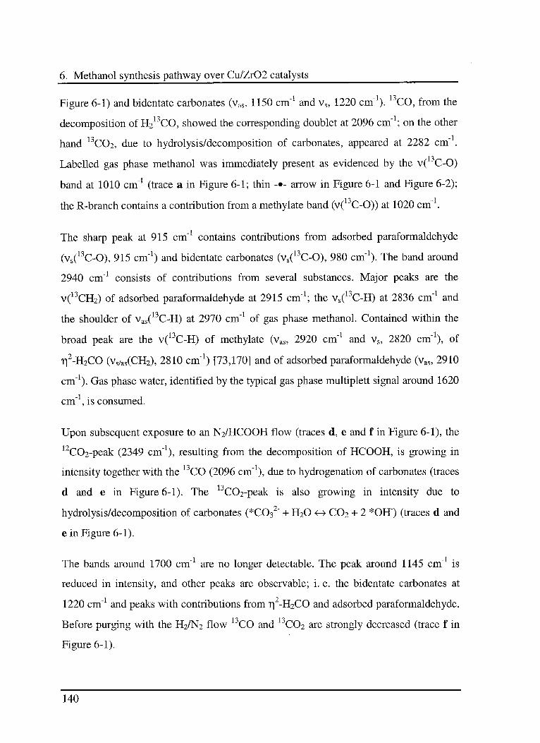
6. Methanol synthesis pathway over Cu/Zr02 catalysts
Figure 6-1) and bidentate carbonates (vas, 1150 cm"1 and vs, 1220 cm"1). 13CO, from the
decomposition of H2 CO, showed the corresponding doublet at 2096 cm" ; on the other
1 o 1
hand C02, due to hydrolysis/decomposition of carbonates, appeared at 2282 cm".
1 ^
Labelled gas phase methanol was immediately present as evidenced by the v( C-O)
band at 1010 cm"1 (trace a in Figure 6-1; thin -•- arrow in Figure 6-1 and Figure 6-2);
the R-branch contains a contribution from a methylate band (v( C-O)) at 1020 cm".
The sharp peak at 915 cm"1 contains contributions from adsorbed paraformaldehyde
(vs(13C-0), 915 cm"1) and bidentate carbonates (vs(13C-0), 980 cm"1). The band around
2940 cm"1 consists of contributions from several substances. Major peaks are the
v(13CH2) of adsorbed paraformaldehyde at 2915 cm"1; the vs(13C-H) at 2836 cm"1 and
the shoulder of vas(13C-H) at 2970 cm"1 of gas phase methanol. Contained within the
broad peak are the v(13C-H) of methylate (vas, 2920 cm"1 and vs, 2820 cm"1), of
r|2-H2CO (vs/as(CH2), 2810 cm"1) [73,170] and of adsorbed paraformaldehyde (vas, 2910
cm"1). Gas phase water, identified by the typical gas phase multiplett signal around 1620
cm"1, is consumed.
Upon subsequent exposure to an N2/HCOOH flow (traces d, e and f in Figure 6-1), the
C02-peak (2349 cm" ), resulting from the decomposition of HCOOH, is growing in
-I Q 1
intensity together with the CO (2096 cm" ), due to hydrogénation of carbonates (traces
d and e in Figure 6-1). The C02~peak is also growing in intensity due to
hydrolysis/decomposition of carbonates (*C032" + H20 <h> C02 + 2 *OH") (traces d and
ein Figure 6-1).
The bands around 1700 cm"1 are no longer detectable. The peak around 1145 cm"1 is
reduced in intensity, and other peaks are observable; i. e. the bidentate carbonates at
1220 cm"1 and peaks with contributions from r|2-H2CO and adsorbed paraformaldehyde.
Before purging with the H2/N2 flow ljCO and 13C02 are strongly decreased (trace f in
Figure 6-1).
140
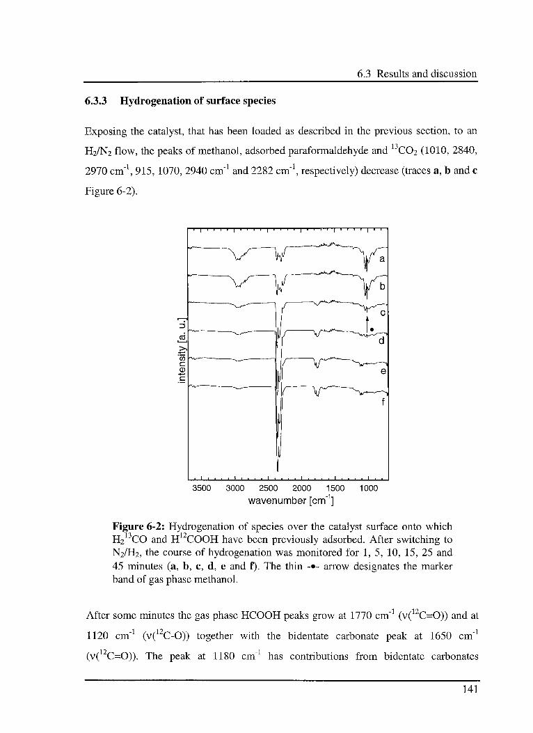
6.3 Results and discussion
6.3.3 Hydrogénation of surface species
Exposing the catalyst, that has been loaded as described in the previous section, to an
H2/N2 flow, the peaks of methanol, adsorbed paraformaldehyde and 13C02 (1010, 2840,
2970 cm"1, 915, 1070, 2940 cm"1 and 2282 cm"1, respectively) decrease (traces a, b and c
Figure 6-2).
3500 3000 2500 2000 1500
wavenumber [cm"1]1000
Figure 6-2: Hydrogénation of species over the catalyst surface onto which13 12
H2 CO and H COOH have been previously adsorbed. After switching to
N2/H2, the course of hydrogénation was monitored for 1, 5, 10, 15, 25 and
45 minutes (a, b, c, d, e and f). The thin -•- arrow designates the marker
band of gas phase methanol.
After some minutes the gas phase HCOOH peaks grow at 1770 cm"1 (v(12C=0)) and at
1120 cm"1 (v(12C-0)) together with the bidentate carbonate peak at 1650 cm"1
(v( C=0)). The peak at 1180 cm" has contributions from bidentate carbonates
141
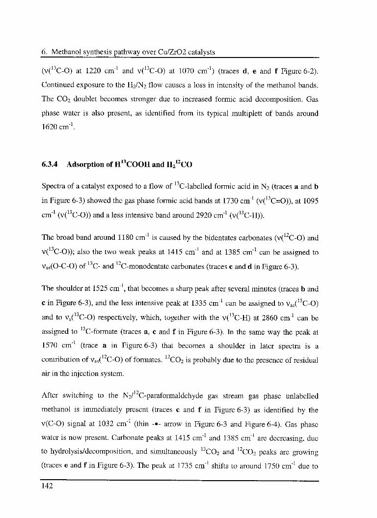
6. Methanol synthesis pathway over Cu/Zr02 catalysts
(v(13C-0) at 1220 cm"1 and v(13C-0) at 1070 cm"1) (traces d, e and f Figure 6-2).
Continued exposure to the H2/N2 flow causes a loss in intensity of the methanol bands.
The CO2 doublet becomes stronger due to increased formic acid decomposition. Gas
phase water is also present, as identified from its typical multiplett of bands around
1620 cm"1.
6.3.4 Adsorption of H13COOH and H212CO
Spectra of a catalyst exposed to a flow of C-labelled formic acid in N2 (traces a and b
in Figure 6-3) showed the gas phase formic acid bands at 1730 cm"1 (v(13C=0)), at 1095
cm"1 (v(13C-0)) and a less intensive band around 2920 cm"1 (v(13C-H)).
The broad band around 1180 cm"1 is caused by the bidentates carbonates (v(12C-0) and
v(13C-0)); also the two weak peaks at 1415 cm"1 and at 1385 cm"1 can be assigned to
vas(0-C-0) of 13C- and 12C-monodentate carbonates (traces c and d in Figure 6-3).
The shoulder at 1525 cm"1, that becomes a sharp peak after several minutes (traces b and
c in Figure 6-3), and the less intensive peak at 1335 cm"1 can be assigned to vas(13C-0)
and to vs(13C-0) respectively, which, together with the v(13C-H) at 2860 cm"1 can be
1 ^
assigned to C-formate (traces a, c and f in Figure 6-3). In the same way the peak at
1570 cm"1 (trace a in Figure 6-3) that becomes a shoulder in later spectra is a
contribution of vas(12C-0) of formates. 12C02 is probably due to the presence of residual
air in the injection system.
After switching to the N2/12C-paraformaldehyde gas stream gas phase unlabelled
methanol is immediately present (traces e and f in Figure 6-3) as identified by the
v(C-O) signal at 1032 cm"1 (thin -•- arrow in Figure 6-3 and Figure 6-4). Gas phase
water is now present. Carbonate peaks at 1415 cm"1 and 1385 cm"1 are decreasing, due
to hydrolysis/decomposition, and simultaneously 13C02 and 12C02 peaks are growing
(traces e and f in Figure 6-3). The peak at 1735 cm"1 shifts to around 1750 cm"1 due to
142
6.3 Results and discussion
19 1contribution of gas phase formaldehyde (v( C=0) at 1755 cm" ). Gas phase
-1 17
paraformaldehyde is also present, as visible from the shoulder at 1210 cm" (v( C-O)).
r)2-H212CO (1155 cm"1) (thick -- arrow in Figure 6-3) is formed and finally becomes
the predominant peak around 1150 cm"1.
3500 3000 2500 2000 1500 1000
wavenumber [cm"1]
rl3Figure 6-3. Adsorption of H COOH for 1, 3 and 5 minutes (a, b and c),12,followed by adsorption of H2 CO for 1, 3 and 5 minutes (d, e and f). The
thin -•- and thick - - arrows designate marker bands of gas phase methanol
and adsorbed formaldehyde, as discussed in text.
The weak peak at 1650 cm"1 can be assigned to the v(C=0) of bidentate carbonates. The
peak around 2950 cm"1 contains contributions from v(C-H) of paraformaldehyde (2915
cm"1) and methanol (2975 cm"1), the peak at 2820 cm"1 is assigned to adsorbed
formaldehyde.
143
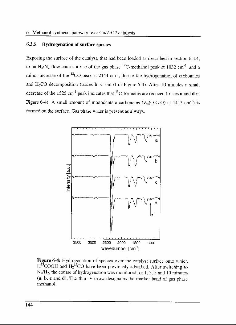
6. Methanol synthesis pathway over Cu/Zr02 catalysts
6.3.5 Hydrogénation of surface species
Exposing the surface of the catalyst, that had been loaded as described m section 6.3.4,
to an H2/N2 flow causes a nse of the gas phase 12C-methanol peak at 1032 cm \ and a
minor increase of the 12CO peak at 2144 cm l, due to the hydrogénation of carbonates
and H2CO decomposition (traces b, c and d m Figure 6-4). After 10 minutes a small
decrease of the 1525 cm"1 peak indicates that 13C-formates are reduced (traces a and d m
Figure 6-4). A small amount of monodentate carbonates (vas(0-C-0) at 1415 cm l) is
formed on the surface. Gas phase water is present as always.
3500 3000 2500 2000 1500 1000
wavenumber [cm1]
Figure 6-4: Hydrogénation of species over the catalyst surface onto which
H13COOH and H212CO have been previously adsorbed. After switching to
N2/H2, the course of hydrogénation was monitored for 1, 3, 5 and 10 minutes
(a, b, c and d). The thin -«-arrow designates the marker band of gas phasemethanol.
144
6.4 Conclusions
6.4 Conclusions
1 "3
In the first described experiment, adsorption of C-labelled paraformaldehyde led to the
formation of adsorbed paraformaldehyde and surface-bound formaldehyde (r|2-H2CO),
which was consumed after switching to the H2/N2. Surface carbonates were formed
from carbon monoxide (13CO), which was generated by H2CO decomposition. In the gas
phase 13C-labelled methanol was clearly detected with its v(13C-0) signal at 1010 cm"1.
1 7
Subsequent adsorption of C-formic acid resulted in the decomposition of HCOOH into
1 3
H2 and C02 and consequently hydrogénation of some carbonates into CO.
Hydrogénation of the surface led to a reduction of all present paraformaldehyde species.
Part of the carbonates were hydrolysed/decomposed to release 13C02; besides, additional
non-reactive carbonates were formed. Labelled methanol was always present. Neither
1 "3
surface bound CO, nor labelled surface formates were observed, even after long
exposure and hydrogénation times. No detectable change in the concentration of surface
hydroxyl groups was observed.
In the second experiment, the adsorption of 13C-labelled formic acid generated surface
carbonates and surface formates. No methanol or methylate signals were observed.
Subsequently, adsorption of H212CO led rapidly to a formation of gas phase unlabelled
CH3OH (v(12C-0) band at 1032 cm"1), and to the hydrolysis/decomposition of
carbonates (rising 13C02 band). No labelled adsorbed paraformaldehyde was detected.
Under reducing atmosphere, a rise of 12CO due to decomposition of H212CO together
with a small decrease of formates and formation of carbonates were observed. No
adsorbed CO was detected. Neither detectable production, nor decrease of surface
hydroxyl groups were observed.
145
6. Methanol synthesis pathway over Cu/Zr02 catalysts
6.4.1 Water gas shift reaction
The observations suggest that CO and C02 can be interconverted via surface carbonates,
according to the equilibria:
CO + 2*OH" <-> *C02 + H2+ *
*C032" <-» *02" + C02
* + *02" + H20 <-> 2 *OH"
where * designates an adsorption site. This scheme is supported by the following
observations. In the first experiment (Figure 6-1) the 13C source is the 13CO. 13C02 and
13C-carbonates must be generated from this source. In the presence of water
(consumption of gas phase water) carbonates will be hydrolysed/decomposed and 13C02
will be formed.
1 7
During the hydrogénation step some C02 is present and a little gas phase water is
consumed (traces e and f in Figure 6-2), as the system is close to equilibrium. In the
second experiment (Figure 6-3) 12C-carbonates are generated from 12C02. During the
17 17
hydrogénation step (Figure 6-4) C-carbonates are reduced and some CO together
with gas phase water is produced. This result is also in agreement with previous
observations [164-168].
6.4.2 Methanol formation
Additional useful information is provided on the methanol synthesis route. The
observations suggest that surface-bound formaldehyde is the key intermediate according
to the equilibria:
*?7-H2CO + *OH" (H2
> *H3CO" + *OH2
*H3CO" + *OH2 <-> * + *OH" + HjCOH
146
6.4 Conclusions
This is supported by the fact that it was not possible to find methylate or methanol
without the presence of ri2-H2CO on the surface (Figure 6-1, Figure 6-3, Figure 6-4),
and that even after long exposure to the hydrogen atmosphere no surface formates
species were reduced to methanol (Figure 6-2 and Figure 6-4), i.e. no methanol was
observed with the same carbon isotope as in the formates.
Most importantly, the isotope of the carbon atom of methanol and of the adsorbed
formaldehyde were always of the same (Figure 6-1, Figure 6-3, Figure 6-4). It was never
possible to observe CO bound to the surface.
Hence, it is possible to conclude that the C-source of the methanol carbon is always the
formaldehyde carbon respectively the ri2-H2CO carbon. This result confirms the
mechanism proposed from previous observations [73,164-168].
147

This is page 148 !
This page was left intentionally blank !
7.1 Introduction
7. Investigation of a complex system
7.1 Introduction
In this chapter the application of the modulation concept to study the reaction pathway
and the reaction rate constants of a complex solid-state catalysed reactions system is
described.
Kinetic data of different reaction steps can be calculated by performing modulation
experiments using different gas feed composition. The dynamic variations in the
concentrations of products, intermediates and reactants are monitored in situ in the
DRIFT cell. The observed phase shift {Ac) is examined depending on the modulation
frequency co. This method is used to derive equilibrium constants and overall rate
constants characterising the investigated reaction steps. By repeating the experiments at
different temperatures, constant such as Arrhenius activation energies can be assessed.
The methanol synthesis starting from H2/CO and H2/CO2 was chosen as test reaction.
As described in sections 4.1 and 6.1, methanol is an important key compound in
chemical industry. Nowadays, CH3OH is mainly produced from H2 and CO and/or C02
(synthesis gas [171]). At first sight, it might be suggested from a stoichiometric point of
view, that carbon monoxide is directly hydrogenated to methanol. The C02
hydrogénation is more complicated, because the reverse water gas shift and the
hydrogénation reactions occur simultaneously (see sections 6.1 and 6.4).
The classical catalysts for the methanol synthesis are based on copper-zinc
oxide-alumina systems. CH3OH synthesis over Cu/ZnO/Al203-based catalysts proceeds
149
7. Investigation of a complex system
via adsorption of carbon dioxide and hydrogen on the surface, to form formate species,
which have been suggested as an intermediate of the methanol synthesis
[172,173,174,175,176] and the water-gas shift reaction [177,178].
The hydrogénation of formates to methoxy-species is considered to be the rate
determining step of the synthesis reaction, which starts from carbon oxides
[179,180,181]. Neophytydes et al. [182] observed that formate species, which are
created by the hydrogénation of carbon dioxide and are adsorbed on copper, are the key
intermediates in the methanol synthesis. Performing experiments with labelled C02,
Chinchen et al. [183] confirmed that C02 is the precursor of methanol.
H2 + 2* <r> 2*H 01
co2 + *<-» *co2 02
*co2 + *<-> *co + *o 03
CO + *<h> *co 04
02 + 2* <-» 2*0 05
*C02 + *H «-> *HCOO + * 06
*HCOO + *H <-» *H2C02 +* 07
*H2C02 + *H <-» *H3CO + *0 08
*H3CO + *H <-» *H3COH +* 09
H3COH + *«-» *H3COH 10
*H2C02 +*o *H2CO + *0 11
H2CO +*^ *H2CO 12
*H2CO + *H O *H3CO + * 13
H20 +*
<-> *H20 14
*H20 +*
<-> *OH + *H 15
*OH + *<-» *0 + *H 16
2*OH +*
<-» *H20 + *0 17
Figure 7-1: Microkinetic reaction model for the methanol synthesis via C02
hydrogénation over Cu(100) [184]. The symbol *represents an adsorption
site.
150
7.1 Introduction
The complete reaction scheme is quite complicated, because several steps, which can be
equilibrium processes, are involved. In Figure 7-1 a complete microkinetic model for
the methanol synthesis via hydrogénation of CO/C02 over Cu(100) is presented [184]. It
is noteworthy that in this model carbonates are not included. Similar models for the
synthesis of CH3OH over Cu single crystal were also proposed by other authors
[133,134].
Previous studies performed on Cu/Zr02-based catalysts by Wokaun and co-workers
[73,155,161-165,185,186] had shown that carbon oxide hydrogénation over
copper/zirconia to yield methanol proceeds via a complete different reaction pathway.
Starting from C02, carbonates and formates are formed rapidly on the reduced surface.
CO32" is hydrogenated to CO and water, whereas the surface formate concentrations
remain in quasi steady state. This step represents the reverse water gas shift reaction.
CO is adsorbed on the surface, hydrogenated, and surface-bound formaldehyde and
formates are generated. Reduction of r|-H2CO leads to the formation of the methylate
and subsequently methanol, whereas surface formates do not react to further
intermediates or products [155] (see also chapter 6).
The reaction pathway of the CH3OH synthesis is divided into different reaction steps to
investigate the overall reaction in more detail. By using C02 it is possible to study the
first part of the reaction, the reverse water gas shift reaction. With CO as reactant, the
second part of the methanol synthesis reaction is examined. First, the CO and C02
adsorption processes are investigated to obtain information about the equilibrium rate
constants and surface species. Then the C02 and CO hydrogénation reactions are
analysed.
The application of zirconia-copper catalysts is of special interest due to their physical
and thermodynamic properties (see chapter 6). A complete review about Cu/Zr02
catalysts can be found elsewhere [187].
151
7. Investigation of a complex system
7.2 Experimental
The used setup is similar to those presented in chapter 5. It consists of the gas dosing
system Modulation Unit connected to the DRIFT cell, which was placed in the FTIR
spectrometer. The whole setup is controlled using the Lab-View based program
presented in section 2.2.
All spectra were recorded in the rapid scan mode with a resolution of 4 cm"1. For
transient measurements, 8 to 64 interferograms per spectrum and 1024 scans for the
background spectra were accumulated.
The amorphous Cu4ôZr54 alloy catalyst for CO oxidation was kindly provided by Prof.
Dr. A. Baiker, and had been prepared as previously described [163]. A certain amount
(0.298 g) of catalyst was placed into the DRIFT sample cup and packed as described in
section 2.4.4 to ensure reproducibility [29-31].
First, some step up/step down test experiments were used to estimate the dead time
between the gas dosing system Modulation Unit and the cell (see paragraph 3.3.4.1) as
well as the ability of the catalyst to propagate a perturbation. In a second step,
modulation experiments were started. The experiment was repeated applying different
temperatures to monitor the influence of the temperature on the reaction. The
concentration changes in step up/step down and modulation experiments exhibited the
same order of magnitude.
Step up/step down and modulation experiments were performed as described in section
5.2. For the same modulation frequency two to four sets of experiments, each consisting
of up to 60 spectra, were collected. The system was held under the same constant initial
conditions for at least 30 minutes, before starting a new modulation experiment. A new
background spectrum was collected for each new experiment. The first two sets of
spectra were discarded, because they contained the initial adjustments of the system to
external perturbations.
152
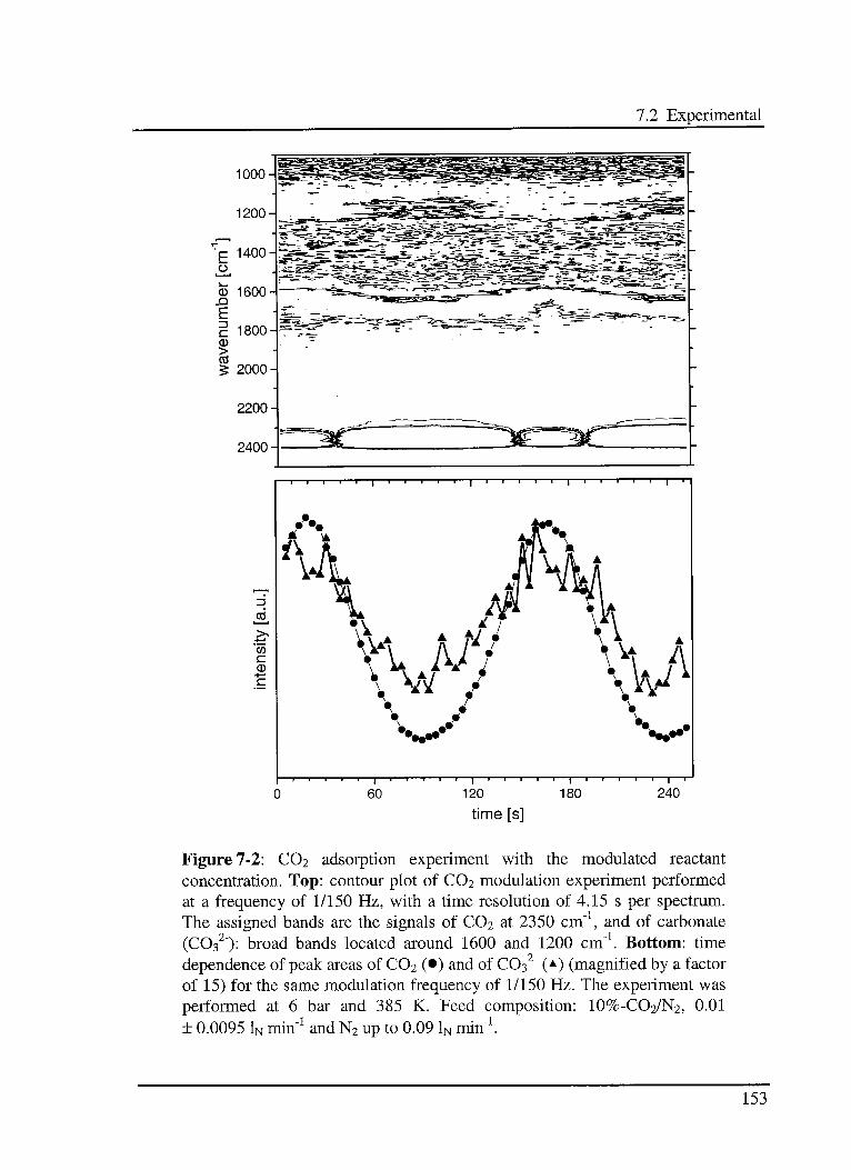
7.2 Experimental
1000-
1200-
T£ 1400
p,
0) 1600
E
c 1800CD>CO
<: 2000
2200
2400
3
cö
0
-| 1 1 1 1 1 1 1 1 1 1 1 1 r- ->—r
»•*•
*M A
v..»
I
60 120
time [s]
180 240
Figure 7-2: CO2 adsorption experiment with the modulated reactant
concentration. Top: contour plot of C02 modulation experiment performedat a frequency of 1/150 Hz, with a time resolution of 4.15 s per spectrum.
The assigned bands are the signals of C02 at 2350 cm"1, and of carbonate
(CO32"): broad bands located around 1600 and 1200 cm"1. Bottom: time
dependence of peak areas of C02 (•) and of CO32" (a) (magnified by a factor
of 15) for the same modulation frequency of 1/150 Hz. The experiment was
performed at 6 bar and 385 K. Feed composition: 10%-CO2/N2, 0.01
± 0.0095 1N min"1 and N2 up to 0.09 1N min"1.
153
7. Investigation of a complex system
The used method to evaluate the collected spectra is described in detail in chapters 3 and
5. The dead time between the gas dosing system and the cell was determined by plotting
the peak area of the modulated gas (CO or C02) as a function of time. The effective
phase shift Acp of other components is deduced by plotting the peak area as a function of
time, which was corrected for the measured dead time. In both cases, a mean value was
calculated from each measured set of data to reduce the error.
In Figure 7-2 (top) a contour plot is shown as example for the obtained spectra during
the C02 adsorption (first recorded trace at the left), where each trace is recorded within
4.15 seconds. At the bottom the corresponding peak area evolutions for the C02
adsorption are shown. The assigned bands are the signals of: C02 (•) at 2350 cm",and
the broad adsorption around 1600 cm"1 [169,182,188] for C032" (a). The used
integration limits are: C02: 2480-2250 cm"1 and C032": 1800-1480 cm"1.
In Figure 7-3 (top) a contour plot and (bottom) the corresponding peak area evolution,
obtained during the CO adsorption experiment, are shown. Each trace is recorded within
4.16 seconds (first recorded trace at the left). The assigned bands are the signals of: CO
() at 2150 cm"1, and adsorbed CO -COad- () at 2040 cm"1. The used integration limits
are: CO: 2250-2065 cm"1 andCOad: 2065-2015 cm"1.
All experiments were performed at a total pressure of 6 bar and at the following
temperatures of 328 K, 385 K, 442 K, 499 K, and 556 K. The feed gas compositions in
the experiments are:
1. C02 adsorption: 10%-CO2/N2, 0.01 ± 0.0095 1N min"1.
2. CO adsorption: 10%-CO/N2, 0.02 ± 0.0195 1N min"1.
3. C02 hydrogénation: 10%-CO2/N2, 0.01 ± 0.0095 1N min"1; H2, 0.02 1N min"1.
4. CO hydrogénation: 10%-CO/N2, 0.02 ± 0.0195 1N min"1; H2, 0.021N min"1.
__
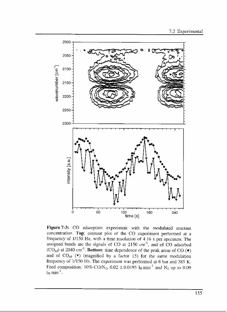
7.2 Experimental
Ep.
CD
E
c
cd>cd
2000
2050-
2100
2150
2200-
2250-
2300
120
time [s]180 240
Figure 7-3: CO adsorption experiment with the modulated reactant
concentration. Top: contour plot of the CO experiment performed at a
frequency of 1/150 Hz, with a time resolution of 4.16 s per spectrum. The
assigned bands are the signals of CO at 2150 cm"1, and of CO adsorbed
(COad) at 2040 cm"1. Bottom: time dependence of the peak areas of CO ()and of COad () (magnified by a factor 15) for the same modulation
frequency of 1/150 Hz. The experiment was performed at 6 bar and 385 K.
Feed composition: 10%-CO/N2, 0.02 ± 0.0195 1N min"1 and N2 up to 0.09
In min"1.
155
7. Investigation of a complex system
Nitrogen was used as carrier and compensation gas. The overall flow was always kept
constant at 0.09 In min"1.
7.3 Results and discussion
As explained in chapter 3, the interpretation of the resulting retardations (phase shifts
Acp or tan[A(/7]) as function of a perturbation (modulation frequency co) is an established
method to obtain information about an unknown system.
A set of equations is used to model the investigated system (see section 3.4). From the
temperature dependence, additional thermodynamic parameters of the reactions are
determined.
The synthesis of methanol can be described by the following microkinetic model:
adsorption of the C-supplying compound (CO or C02), adsorption and dissociation of
hydrogen, reaction between the C-containing surface species and hydrogen to form
intermediates, which react further to form new intermediates, and so on. The end
products are methanol and, for C02, also water. The interactions of CO and C02 with
the catalyst in an inert and hydrogen containing atmosphere are analysed separately, to
estimate the kinetic data characteristic of each reaction step.
For all experiments the C-supplying reactant (CO or C02) was modulated.
Unfortunately, only modifications in the concentration of the first surface species could
be detected. It was, however, not possible to deduce any phase shift between gas phase
and surface species within an acceptable error, because the signal of the adsorbed
species was always in phase with the signal of the reactant in the gas phase (see also
Figure 7-2 and Figure 7-3). Test experiments using higher modulation frequencies were
performed to resolve the phase shifts. The resulting amplitude of the concentration
variation was unfortunately not large enough to define the retardation.
156
7.3 Results and discussion
Additional test experiments with higher amplitudes and longer periods were performed
for the C02 and CO hydrogénation reactions to study the perturbation of further
intermediates and products. The resulting signals were again not strong enough to
identify these compounds or to define a retardation A #? within an acceptable error.
7.3.1 C02 adsorption on the reduced catalyst
7.3.1.1 Model
A modulation experiment was carried out to estimate the interaction of a reactant gas
(C02) with the catalyst surface (see section 7.3.2). Under the used conditions it was not
possible to distinguish between carbonite (CO2 ), which has the asymmetric stretching
vibration around 1540 cm"1 [185,189,190] and carbonates, which have a broad
absorption band around 1600 cm"1. The existence of carbonates on the surface was
confirmed by the presence of the bands around 1200 cm"1 [185]. However, this does not
exclude the existence of CO2"
species on the surface at concentrations below the
detection limit of DRIFT, or as high frequency part of the carbonate bands at 1600 cm"1.
The used model implies that carbon dioxide adsorbs and generates carbonates [73]
immediately. To obtain a better propagation of the perturbation, the largest possible
amplitude was used. The lowest possible partial pressure was applied in order to avoid
unwanted effects, such as saturation of the surface as well as an influence of the
concentration of vacant adsorption sites. Applying a reduced carbon dioxide partial
pressure has the consequence that the changes in the gas phase concentration are
limited. Therefore, it is possible to assume that the surface coverage is low and that the
number of vacant CO2 adsorption site remains quasi constant. The following simple
model can be derived:
157
7. Investigation of a complex system
k
C02 ^ C02-k-1
Here, k\ and k.\ are effective first order rate constants. As explained in section 3.3.2, the
DRIFT cell can be represented by a continuous stirred tank reactor with a residence time
t. Therefore, the system can be described with the following set of differential
equations:
dÇO^CO^. (fc +I)C02 + Jk ^O*" (7.1)
dt T T
dCO\-dt
= kxC02 - fc_1C032" (7.2)
C02,o represents the gas phase concentration of carbon dioxide in the feed gas and C02
in the DRIFT cell, CO32" is the surface concentration of carbonates. The set of
differential equations is solved for C02 and C032". Equations as function of co and co2
(see Equation 3.28) are obtained. As explained in paragraph 3.A..2.1, the co2 terms are
only important when high frequencies are applied. Therefore, the low frequency
approximation can be applied and the linearity between the tangent of the phase shift
(tan[A#>]) and the perturbation frequency (u)) is obtained:
tan [Acp{CO2Q-CO2)\ = C0T{\ + ^-) (7.3)
tan [ç{C02)-cp{COl-)] = ^- (7.4)k,
In Equation 7.3 an equilibrium constant k\lk.\ appears, rather than an individual rate
constant as in Equation 7.4 (see paragraph 3.4.2.1). The temperature influence was
estimated, as explained in chapter 3. The residence time (1) is modelled using Equation
3.9, which was derived from ideal gas law (see Equation 3.8). For the rate constants k\
158
7.3 Results and discussion
and fc_i the Arrhenius Equation was used (see Equation 3.10). The pre-exponential factor
ko was assumed to be temperature independent.
t{T) =^- (3.9)
-Ma
k{T) = k0e RT (3.10)
As explained in section 5.3.1 the equilibrium constant K{T) of the reaction can be easily
derived from Equation 3.10:
k -^
K(T) =J^
= KoeRT (5.5)
k-i
Here AEa is the difference of the Arrhenius activation energies between the adsorption
and desorption process. The sign of AEa indicates whether the equilibrium process
favours reactants or products.
7.3.1.2 Experimental results
In Figure 7-2 a contour plot and the peak area evolution for a C02 adsorption
experiment are shown. An example for the evolution of the phase shifts as a function of
the modulation frequencies is illustrated in Figure 7-4. Open triangles (a) display the
frequency dependence of tan[Aç7(CO2;0-CO2)] found for the lowest applied temperature
(328 K), and filled triangles (a) for the highest temperature (556 K). As expected, the
phase shifts can be approximated by straight lines with zero crossing. The arrow
indicates the direction of the slope change caused by increasing temperatures.
The obtained slope contains information about the reaction {K\$ and A£a,i) as well as
the residence time {k^). The evolution of the slope values as function of temperature is
shown in Figure 7-5. A monotonous temperature dependence of the adsorption/
159
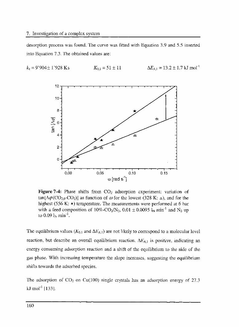
7. Investigation of a complex system
desorption process was found. The curve was fitted with Equation 3.9 and 5.5 inserted
into Equation 7.3. The obtained values are:
Jku = 9'904±l'928Ks £0li = 51±ll AEA,i = 13.2 ± 1.7 kJ mol"1
-\ 1 1 1— l | 1 1 T— 1-
|" "T I
"—I '"T | 1
0.00 0.05 0.10 0.15
co [rad s"1]
Figure 7-4: Phase shifts from C02 adsorption experiment: variation of
tan[A<p(C02,o-C02)] as function of co for the lowest (328 K: a), and for the
highest (556 K: *) temperature. The measurements were performed at 6 bar
with a feed composition of 10%-CO2/N2, 0.01 ± 0.0095 1N min"1 and N2 up
to 0.09 1N min"1.
The equilibrium values (Ko,i and AEA,i) are not likely to correspond to a molecular level
reaction, but describe an overall equilibrium reaction. AE^i is positive, indicating an
energy consuming adsorption reaction and a shift of the equilibrium to the side of the
gas phase. With increasing temperature the slope increases, suggesting the equilibrium
shifts towards the adsorbed species.
The adsorption of C02 on Cu(100) single crystals has an adsorption energy of 27.3
kJ mol"1 [133].
160
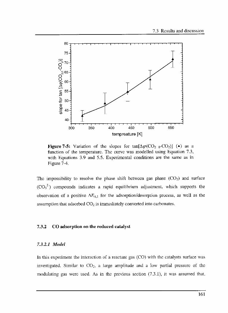
7.3 Results and discussion
80-
75-
70-
^65-
60-
OO
c
c.
oo
e-<
c 55cd-t—«
O 50-
CDQ.
o 45.CO
40-
-i j 1 1—1 r—j 1—1 1 1 T" 1 1 1 11 1 1—
300 350 400 450
i—1 1 1 1 1 1—p—r-
500 550
tempreature [K]
Figure 7-5: Variation of the slopes for tan[A#?(C02 o-C02)] (±) as a
function of the temperature. The curve was modelled using Equation 7.3,
with Equations 3.9 and 5.5. Experimental conditions are the same as in
Figure 7-4.
The impossibility to resolve the phase shift between gas phase (C02) and surface
(CO32) compounds indicates a rapid equilibrium adjustment, which supports the
observation of a positive AEA,\ for the adsorption/desorption process, as well as the
assumption that adsorbed C02 is immediately converted into carbonates.
7.3.2 CO adsorption on the reduced catalyst
7.3.2.1 Model
In this experiment the interaction of a reactant gas (CO) with the catalysts surface was
investigated. Similar to C02, a large amplitude and a low partial pressure of the
modulating gas were used. As in the previous section (7.3.1), it was assumed that,
161
7. Investigation of a complex system
during the experiment, the surface concentration of vacant CO adsorption sites was
constant.
An additional advantage of a low partial pressure is the reduced influence of the carbon
monoxide gas phase signal (2150 cm"1) on the quality of CO surface signal (2040 cm"1).
For large modulation amplitudes, no strong changes in the intensity of the CO band are
induced.
The simplified model can be written as:
h
CO ^=^ coad
k-3
The same assumptions are also valid in this case: a) k3 and k.3 are effective first order
rate constants, and b) the DRIFT cell can be represented by a continuous stirred tank
reactor with the residence time t. According to these assumptions, the system can be
describe using Equations 7.1 and 7.2, where, C02 should be substituted by CO, k\ with
k3 and fe_i with k.3.
^- = ^±-{k3 +1) CO + fc_3COad (7.5)dt T T
^L= k3CO-k_3COid (7.6)dt
where COo represents the CO concentration in the feed gas, CO the concentration of
carbon monoxide in the DRIFT cell, and COad the concentration of the adsorbed species.
Equations 7.5 and 7.6 are solved under the same assumptions as in the previous section
for C02. Linear relations between the tangent of the phase shift and the modulation
frequency are obtained:
162
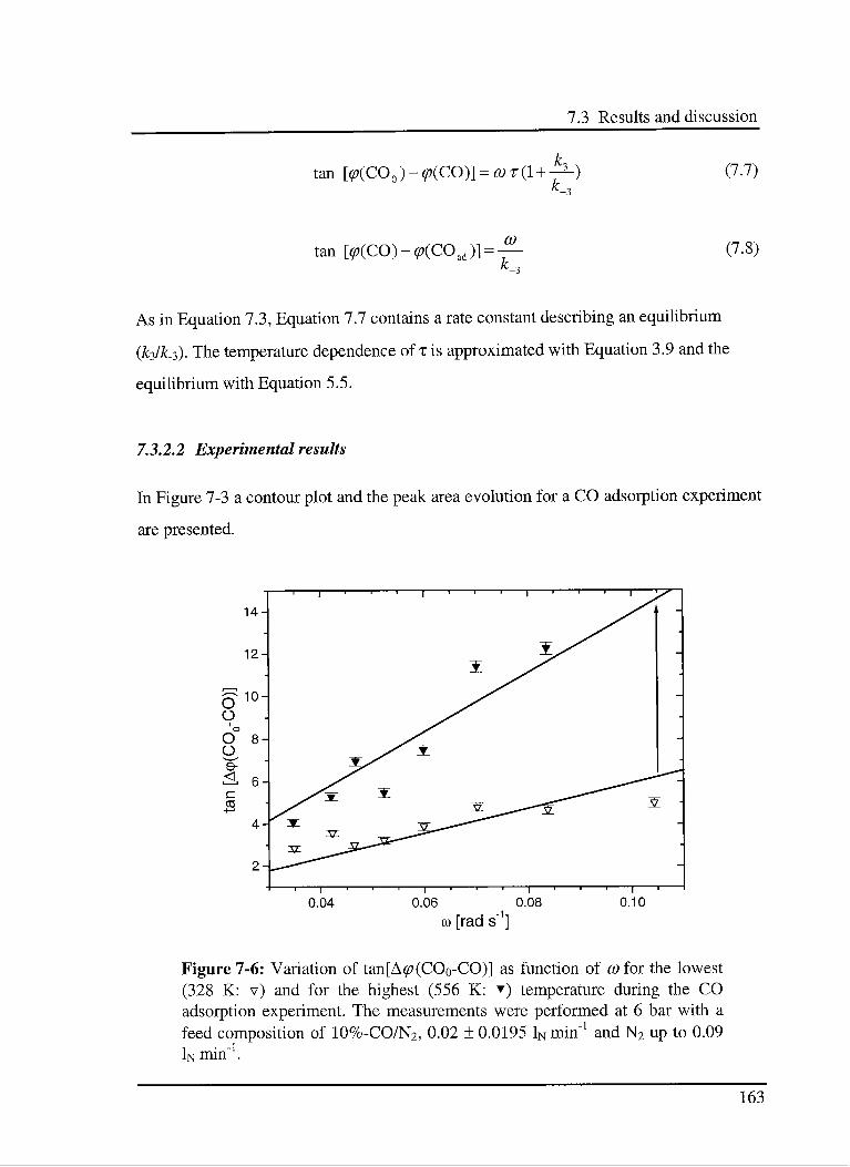
7.3 Results and discussion
tan [p(CO0)-p(CO)] = û>r(l + -3-) (7.7)
co
tan [<p(CO)-<p(COad)] =— (7.8)
As in Equation 7.3, Equation 7.7 contains a rate constant describing an equilibrium
{k3/k.3). The temperature dependence of x is approximated with Equation 3.9 and the
equilibrium with Equation 5.5.
7.3.2.2 Experimental results
In Figure 7-3 a contour plot and the peak area evolution for a CO adsorption experiment
are presented.
0.04 0.06 0.08 0.10
co [rad s"
Figure 7-6: Variation of tan[A^(CO0-CO)] as function of co fox the lowest
(328 K: v) and for the highest (556 K: ) temperature during the CO
adsorption experiment. The measurements were performed at 6 bar with a
feed composition of 10%-CO/N2, 0.02 ± 0.0195 1N min"1 and N2 up to 0.09
In min"1.
163
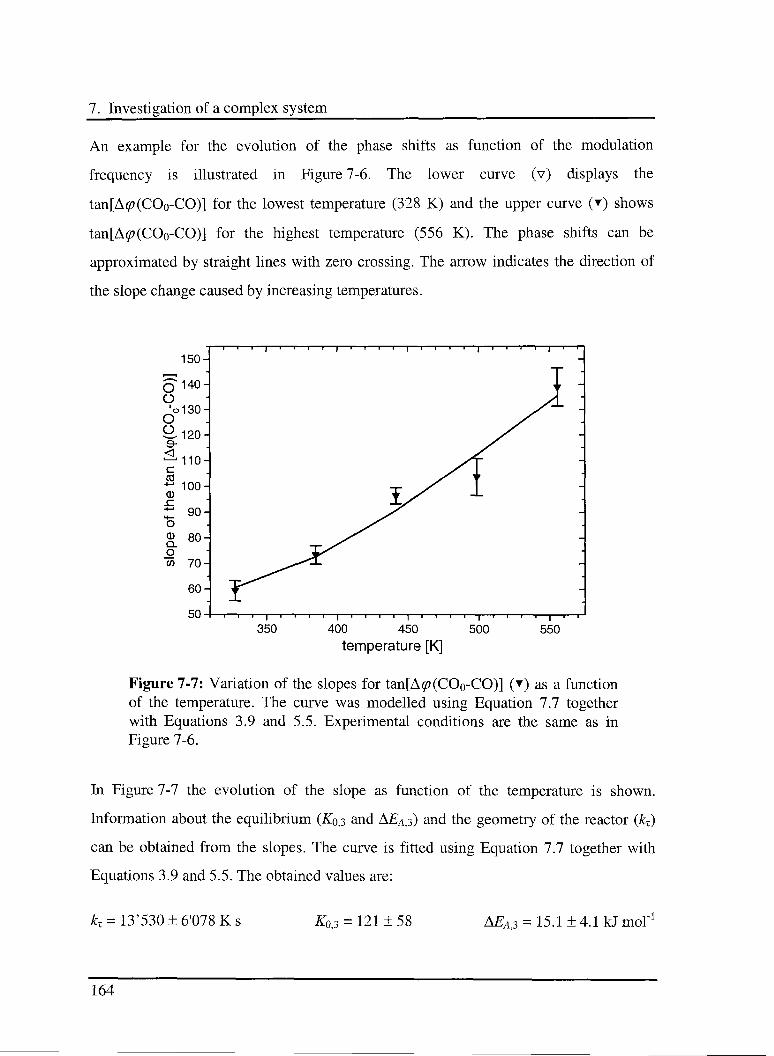
7. Investigation of a complex system
An example for the evolution of the phase shifts as function of the modulation
frequency is illustrated in Figure 7-6. The lower curve (v) displays the
tan[A#?(COo-CO)] for the lowest temperature (328 K) and the upper curve () shows
tan[Acp(CO0-CO)] for the highest temperature (556 K). The phase shifts can be
approximated by straight lines with zero crossing. The arrow indicates the direction of
the slope change caused by increasing temperatures.
150-111)1111 1 1 I 1 1 | 1 1 1 T—1 1 1 1 1 1 1 1
, ,
5*140- i r
Ü'o130- >^^^
_
O yT9-120- JS
e-<
..
"110--
c
cd yTi r
~ 100-0 1/ l :
Z 9°- _
o
S 80- _
Q.O -
co 70- -
60- -
50- 1 1 1 | 1 1 1 | 1—> 1— T , "I P 1 1— 1 1 1 1 1 1 1 1
350 400 450 500
temperature [K]
550
Figure 7-7: Variation of the slopes for tan[A<p(COo-CO)] () as a function
of the temperature. The curve was modelled using Equation 7.7 togetherwith Equations 3.9 and 5.5. Experimental conditions are the same as in
Figure 7-6.
In Figure 7-7 the evolution of the slope as function of the temperature is shown.
Information about the equilibrium (Xo,3 and AEA,3) and the geometry of the reactor {kx)
can be obtained from the slopes. The curve is fitted using Equation 7.7 together with
Equations 3.9 and 5.5. The obtained values are:
^=13'530±6'078Ks Z0,3 = 121 ± 58 AE^s = 15.1 ±4.1 kJ mol"
164
7.3 Results and discussion
The expectancy value for k^ differs slightly from the value obtained for the C02
adsorption/desorption process in the previous experiment (see section 7.3.1). The
difference is probably due to the reduced quality of the data. This hypothesis is
supported by the large standard deviations, making the difference between the two k^
values insignificant.
It is noteworthy that the adsorption energy obtained in this experiment (15.1 kJ mol" ) is
very different from the value (= 53.9 kJ mol"1) of CO on Cu(100), Cu(llO) or Cu(lll)
[133]. The large difference between the values indicates an important influence of the
support (zirconia) on the physico-chemical characteristic of the copper catalyst.
The positive value of AEA,3 suggests that the adsorption reaction is energy consuming
and that the equilibrium is on the side of the gas phase compound. The increase of the
slope, with increasing temperature, indicates a shift of the equilibrium towards the
adsorbed species. This result agrees with the observation that, in absence of gas phase
CO, the COad concentration decreases rapidly below the detection limit (data not
shown). Chorkendorff et al. have demonstrated, by using temperature programmed
desorption experiments in ultra high vacuum (TPD-UHV), that on a pure copper single
crystal (100) no carbon monoxide can be adsorbed on the surface at temperatures above
293 K [191,192].
The evidence that the signals of CO and COad are always in phase (see also Figure 7-3)
confirms the rapid equilibrium adjustment between the two species and supports the
observation of a positive AEa,3-
165
7. Investigation of a complex system
7.3.3 C02 hydrogénation reaction
7.3.3.1 Model
This modulation experiment was carried out to investigate the influence of the carbon
dioxide during CO2 hydrogénation reaction over the Cu/ZrC^-based catalyst.
Several authors report [161-165,185,186] that the C02 hydrogénation over these
catalysts has the following reaction pathway: C02 adsorbs on the reduced surface,
generating formates and carbonates. Carbonates are converted to CO via the reverse
water gas shift reaction. Subsequent hydrogénation of adsorbed carbon monoxide results
in the formation of surface-bound formaldehyde and methylate. No reaction of formates
to further intermediates or products could be detected [155] (see also chapter 6).
The following assumptions were made to assess a simplified model for
C02-modulation.
(1) As explained in section 7.3.1, it was not possible under the used conditions to
discriminate between carbonite (C02 ) and carbonates (CO3 "). It is assumed that gas
phase carbon dioxide is adsorbed and forms immediately carbonates.
(2) It is assumed that the CO32" decomposition process to C02 is much faster than the
carbonates hydrogénation reaction, which results in an undefined surface intermediate
species [#].
The validity of these assumptions is supported by the evidence that the applied
perturbations do not propagate observably further along the reaction pathway; and no
changes of formates, surface-bound formaldehyde and methylate bands could be
detected. Only the concentrations of carbon dioxide and carbonates are changing.
(3) H2 is used in excess. This allows the assumption of a saturation of hydrogen on
the surface. As a consequence the rate constants of the different reaction steps are not
166
7.3 Results and discussion
dependent on hydrogen surface concentration. Furthermore, the equilibrium of any
reversible hydrogénation reaction step would be shifted towards the product side, and
any possible dehydrogenation (reverse) reactions would be inhibited. Therefore, an
overall first order rate constant {k2) describing the CO32" hydrogénation reaction was
used.
A low C02 partial pressure and a large amplitude are used and a quasi constant
concentration of vacant C02 adsorption sites is assumed (see section 7.3.2). A simple
model is chosen to describe the reaction.
k
2
co2 .
» co32" —'-*- [#]
k\, k-i and k2 are effective first order rate constants. As explained in section 3.3.2 the
DRIFT cell is represented by a continuous stirred tank reactor with residence time T.
With these assumptions the system can be modelled using differential equations 7.1 and
7.9.
^ço1=co2^_ (Jki+I)C0 +kiC02- (71)
dt T T
dCO2'
dt^C02 - (£_! + k2') C03" (7.9)
Solving this system for C02 and CO32", with the same procedure as in the previous
sections and assuming k.\ » k2 (see assumption 2 above) the phase shifts can be written
as:
(1 + fL)tan [A<?(CO20-CO2)] = ö; -± (7.10)
{T~l+^-k2)
167
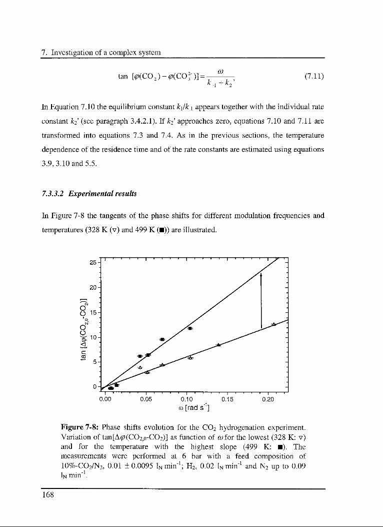
7. Investigation of a complex system
tan [ç{C02)-ç{C023)] =
co
/C i "T~ K-^y
(7.11)
In Equation 7.10 the equilibrium constant k\lk.\ appears together with the individual rate
constant k2 (see paragraph 3.4.2.1). If k2 approaches zero, equations 7.10 and 7.11 are
transformed into equations 7.3 and 7.4. As in the previous sections, the temperature
dependence of the residence time and of the rate constants are estimated using equations
3.9, 3.10 and 5.5.
7.3.3.2 Experimental results
In Figure 7-8 the tangents of the phase shifts for different modulation frequencies and
temperatures (328 K (v) and 499 K ()) are illustrated.
25-
20-
8 15-i
o
oÜ
s-
<[c
cd
10-
i i r- I I I I i i 1 r~
0.00 0.05 0.10
cd [rad s"1]0.15 0.20
Figure 7-8: Phase shifts evolution for the C02 hydrogénation experiment.Variation of tan[A<p(CO2,0-CO2)] as function of «for the lowest (328 K: v)and for the temperature with the highest slope (499 K: ). The
measurements were performed at 6 bar with a feed composition of
10%-CO2/N2, 0.01 ±0.0095 lNmin"1; H2, 0.02 ^min"1 and N2 up to 0.09
In min".
168
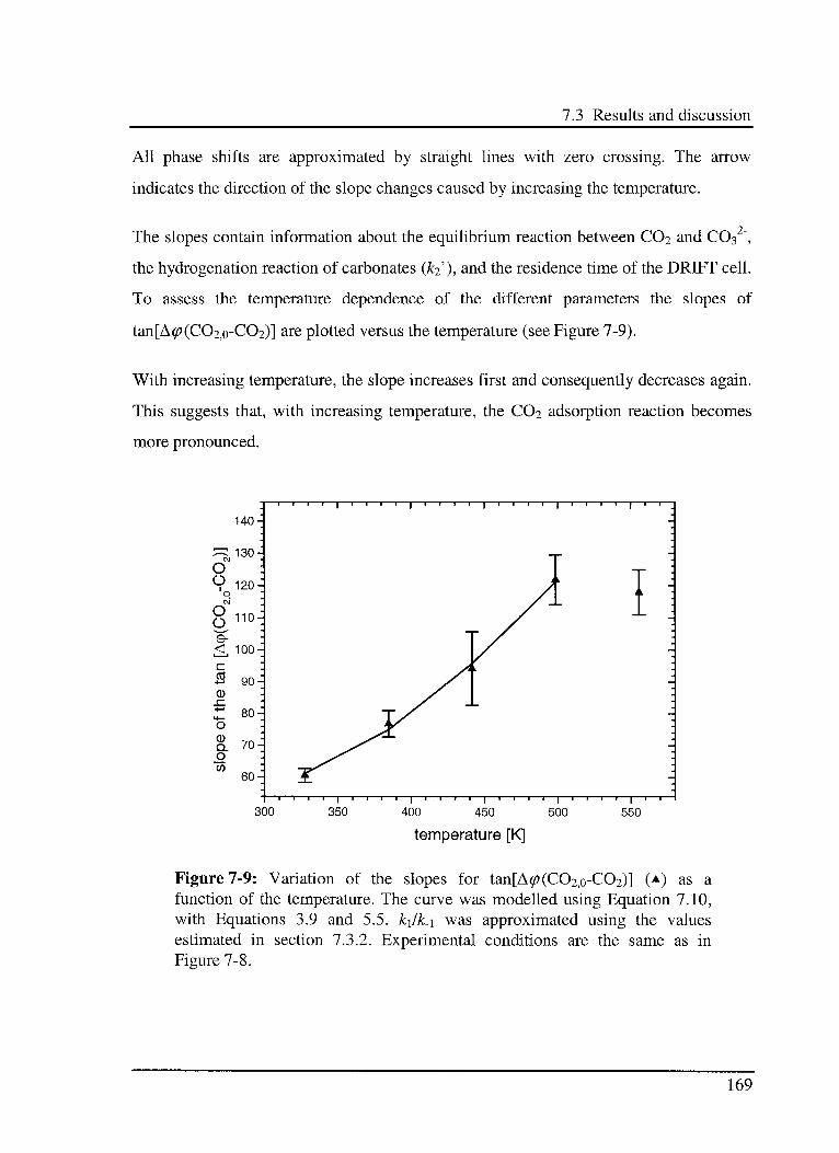
7.3 Results and discussion
All phase shifts are approximated by straight lines with zero crossing. The arrow
indicates the direction of the slope changes caused by increasing the temperature.
The slopes contain information about the equilibrium reaction between C02 and CO3 ",
the hydrogénation reaction of carbonates (k2), and the residence time of the DRIFT cell.
To assess the temperature dependence of the different parameters the slopes of
tan[Ac?(C02,o-C02)] are plotted versus the temperature (see Figure 7-9).
With increasing temperature, the slope increases first and consequently decreases again.
This suggests that, with increasing temperature, the CO2 adsorption reaction becomes
more pronounced.
140-
>—.
130-C\J
Ü -
Ü 1?0-0
"
OJ
00 110-|
9-<1 100-
c"
cd90-
0) .
_c1—'
H—80-
O -
CDO 70-
O .
CO
60-
300 350 400 450 500 550
temperature [K]
Figure 7-9: Variation of the slopes for tan[A^(C02,o-C02)] (A) as a
function of the temperature. The curve was modelled using Equation 7.10,
with Equations 3.9 and 5.5. k\lk.\ was approximated using the values
estimated in section 7.3.2. Experimental conditions are the same as in
Figure 7-8.
169
7. Investigation of a complex system
Using temperatures above 500 K another reaction becomes more pronounced. In section
7.3.1 the evolution of the adsorption/desorption reaction was not found to indicate an
increased desorption for the higher temperatures (556 K). Therefore, an increase in the
carbonate hydrogénation reaction can be deduced.
In a first step, the curve plotted in Figure 7-9 was fitted using equations 3.9, 3.10 and
5.5 substituted in equation 7.10. The values describing the equilibrium between CO2 in
the gas phase and on the surface (&1/&-1) were substituted by the parameters estimated in
section 7.3.1. The parameters deduced from the fit would suggest an enhanced
dehydrogenation (£0,2' < 0) of the undefined intermediates [#], indicating that the applied
model is not adequate.
Therefore, it was assumed that the carbonate hydrogénation reaction can be neglected
{k2~0). The curve shown in Figure 7-9 was fitted using equation 7.3. Due to this
simplification assumption 3 is not any longer valid. New parameters describing the
adsorption/desorption equilibrium {k{k.\) are estimated. The obtained values are:
&T=13'497±2'787Ks £0,1'= 151 ±50 AEA,i = 15.6 ± 2.3 kJ mol"1
The calculated activation energy {AEa,{) is close to the value obtained in the previous
section (7.3.1) for the CO2 adsorption, suggesting that the CO32" hydrogénation reaction
is of minor importance, and that an adsorption/desorption equilibrium is the dominant
process. This result confirms assumptions 1 and 2. The values of the pre-exponential
factor CRTo,i') and residence time {kz) have a large standard deviation. This is probably
due to the presence of hydrogen, and represents an indirect evidence for a CO32"
hydrogénation reaction.
The C03"
and CO2 signals are always in phase, suggesting that the equilibrium between
these two species is the dominant step. This observation confirms also the validity of
assumptions 1 and 2.
170
7.3 Results and discussion
7.3.4 CO hydrogénation reaction
7.3.4.1 Model
The modulation experiment was carried out to investigate under reaction conditions the
interaction between CO and the surface of the Cu/Zr02 catalyst. As reported by several
authors [161-165,185,186] CO is adsorbed on the surface of the catalyst, then reduced to
surface-bound formaldehyde and subsequently to methoxy species. The generated
formates show an improved stability even in a strong reducing atmosphere [185].
To assess a simplified model for CO-modulation experiments, the following
assumptions are made.
(1) Adsorbed carbon monoxide (COad) can desorb or react with hydrogen surface
groups to form an undefined surface species [#]. The desorption process is much faster
than the COad hydrogénation reaction.
The validity of this assumption is supported by the fact that perturbations do not
propagate along the reaction pathway observably. Only changes in the concentration of
COad can be clearly monitored, whereas modification of other surface species
concentration can not be detected.
(2) Using an excess of H2 allows one to assume a saturation of hydrogen on the
surface. As a consequence, the rate constants of the different reaction steps are not
dependent on the hydrogen surface concentration. Furthermore, each hydrogénation
reaction step is shifted towards the product side, and any possible dehydrogenation
(reverse) reaction is inhibited. Therefore, an overall first order rate constant (£4') can be
used to describe the COad hydrogénation reaction.
As in the previous section a large amplitude and a low CO partial pressure are applied,
and a quasi constant concentration of vacant CO adsorption sites is assumed. In view of
these limitations a simple reduced model can be chosen.
171
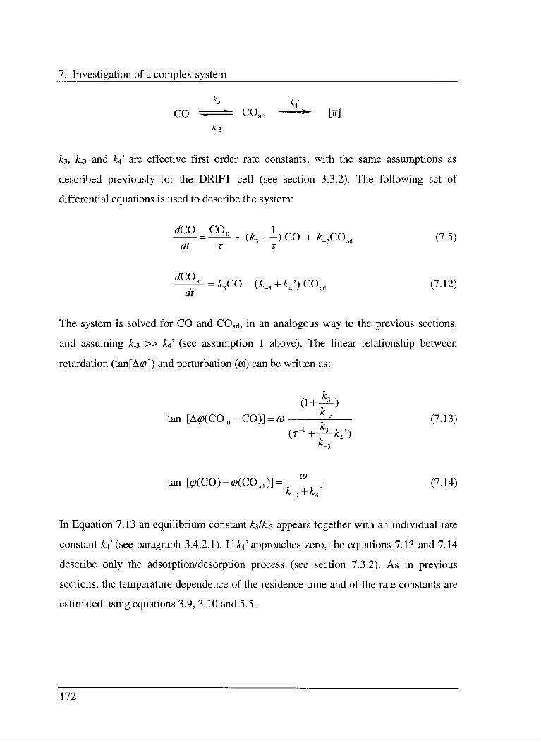
7. Investigation of a complex system
k3£4>
CO ^^ coad [#]
k-3
k3, k.3 and fc4' are effective first order rate constants, with the same assumptions as
described previously for the DRIFT cell (see section 3.3.2). The following set of
differential equations is used to describe the system:
^=^2°.
. {k3 +I) CO + k_3COäd (7.5)dt T T
dCO
dt
^= k3CO- (£_3+£4')COad (7.12)
The system is solved for CO and COad, in an analogous way to the previous sections,
and assuming k.3 » fc4' (see assumption 1 above). The linear relationship between
retardation (tan[A#>]) and perturbation (co) can be written as:
(1+F~}tan [Acp{CO0-CO)] = co f± (7.13)
tan [<?(CO)-«?(COad)]= \ ,(7.14)
In Equation 7.13 an equilibrium constant £3/^3 appears together with an individual rate
constant k\ (see paragraph 3.4.2.1). If &4' approaches zero, the equations 7.13 and 7.14
describe only the adsorption/desorption process (see section 7.3.2). As in previous
sections, the temperature dependence of the residence time and of the rate constants are
estimated using equations 3.9, 3.10 and 5.5.
172
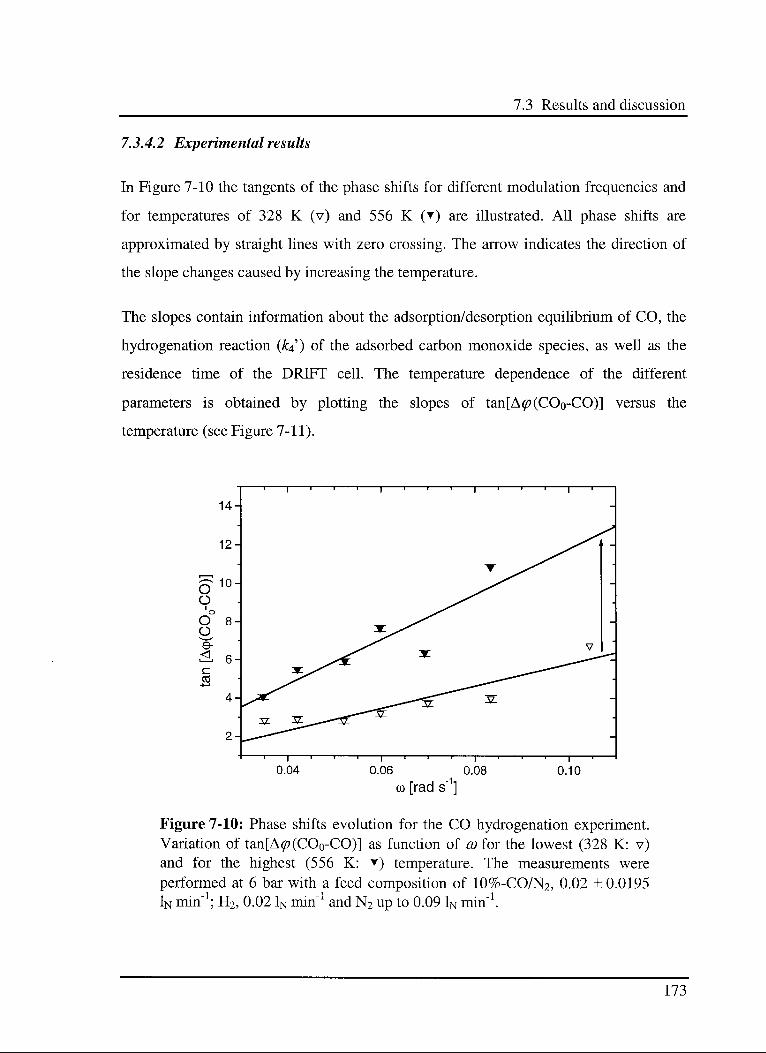
7.3 Results and discussion
7.3.4.2 Experimental results
In Figure 7-10 the tangents of the phase shifts for different modulation frequencies and
for temperatures of 328 K (v) and 556 K () are illustrated. All phase shifts are
approximated by straight lines with zero crossing. The arrow indicates the direction of
the slope changes caused by increasing the temperature.
The slopes contain information about the adsorption/desorption equilibrium of CO, the
hydrogénation reaction (&4') of the adsorbed carbon monoxide species, as well as the
residence time of the DRIFT cell. The temperature dependence of the different
parameters is obtained by plotting the slopes of tan[A<p(COo-CO)] versus the
temperature (see Figure 7-11).
14-
l l l l l i 1 1 l l 1 1 r-
0.04 0.06 0.08 0.10
co [rad s" ]
Figure 7-10: Phase shifts evolution for the CO hydrogénation experiment.Variation of tan[A^(CO0-CO)] as function of co for the lowest (328 K: v)and for the highest (556 K: ) temperature. The measurements were
performed at 6 bar with a feed composition of 10%-CO/N2, 0.02 ± 0.0195
1N min"1; H2, 0.02 1N min"1 and N2 up to 0.09 1N min"1.
173
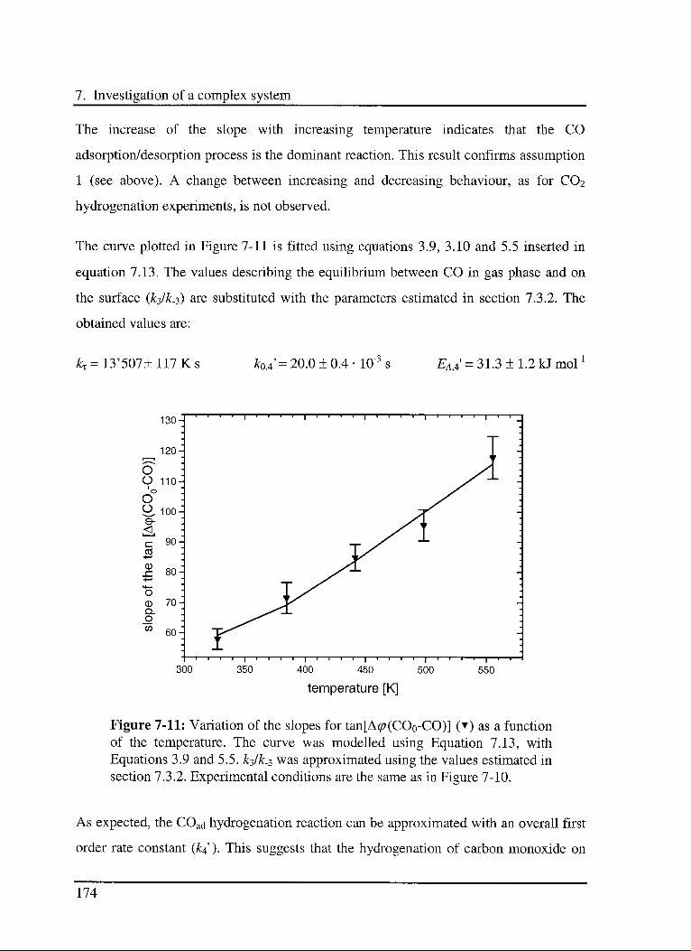
7. Investigation of a complex system
The increase of the slope with increasing temperature indicates that the CO
adsorption/desorption process is the dominant reaction. This result confirms assumption
1 (see above). A change between increasing and decreasing behaviour, as for C02
hydrogénation experiments, is not observed.
The curve plotted in Figure 7-11 is fitted using equations 3.9, 3.10 and 5.5 inserted in
equation 7.13. The values describing the equilibrium between CO in gas phase and on
the surface {k3lk.3) are substituted with the parameters estimated in section 7.3.2. The
obtained values are:
fcl=13'507±117Ks ko/= 20.0 ±0.4- 10"3s Eaa = 31.3 ± 1.2 kl mol"1
130- —1—1—1—1—|—1—1—1—1—|—1—1—1—1—|—1—1—1—1—1 ' ' 1 1 | 1 1_
120- j1—1
- ' ' "i
0 -
0 \-\o- ^r-*-
_
0
0 '.
0 100-J -
< yS ' ' \1 1
c 90 -_-
cd ;-»—'
.
0) .
.c 80- -
-t—»_^
^^^*+—
0
CD 70'.1 1/T _
Q.
O ^»^-~ '_CO
60-j
1 1 1 1 1 1 1 1 1 | 1 1 1 1 1 1 I 1 1 1 ' ' r 1 i 1 1 1
300 350 400 450 500
temperature [K]
550
Figure 7-11: Variation of the slopes for tan[A<p(CO0-CO)] () as a function
of the temperature. The curve was modelled using Equation 7.13, with
Equations 3.9 and 5.5. k3lk.3 was approximated using the values estimated in
section 7.3.2. Experimental conditions are the same as in Figure 7-10.
As expected, the COad hydrogénation reaction can be approximated with an overall first
order rate constant (£4 ). This suggests that the hydrogénation of carbon monoxide on
174
7.4 Conclusions
the surface is faster than the dehydrogenation of the intermediate [#]. This confirms
assumption 2 (see above).
The signals of CO and COad are always in phase, indicating a rapid equilibrium
adjustment between the two species. This result suggests that the desorption reaction
should be at least fast as the COad hydrogénation, again confirming assumption 1 (see
above). If the hydrogénation process would be faster the slopes for tan[A<p(COo-CO)]
would decrease with increasing temperature (see section 5.3.3).
7.4 Conclusions
7.4.1 Methanol synthesis via hydrogénation of CO
Tracing the propagation of perturbations along the reaction pathway is very difficult. For
modulation of carbon monoxide in the gas phase, oscillatory components in the DRIFT
signals could be detected only for adsorbed CO (COad). Gas phase and surface CO are
always in equilibrium, as demonstrated by the problems to estimate a rate constant for
the desorption reaction. In the presence of hydrogen, the existence of an intermediate,
which is formed by hydrogénation of COad, is supported by the fact that it is possible to
estimate the rate constant k\. The nature of the latter intermediate [#] could not be
established from the present experiment due to a strong attenuation of the propagated
modulation amplitudes.
Test experiments with modifications of hydrogen concentration were used to investigate
whether the signals of the intermediates remain insensitive to perturbations. Hydrogen is
active in several steps of the reaction pathway (see Figure 7-1). Therefore, changes in
the H2 concentration would be expected to induce modifications of surface
concentration of various compounds (see chapter 4). As example, the peak area
175
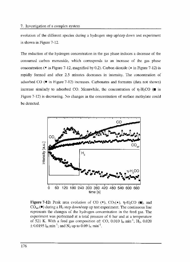
7. Investigation of a complex system
evolution of the different species during a hydrogen step up/step down test experiment
is shown in Figure 7-12.
The reduction of the hydrogen concentration in the gas phase induces a decrease of the
consumed carbon monoxide, which corresponds to an increase of the gas phase
concentration ( in Figure 7-12, magnified by 0.2). Carbon dioxide (± in Figure 7-12) is
rapidly formed and after 2.5 minutes decreases in intensity. The concentration of
adsorbed CO (• in Figure 7-12) increases. Carbonates and formates (data not shown)
increase similarly to adsorbed CO. Meanwhile, the concentration of r|-H2CO ( in
Figure 7-12) is decreasing. No changes in the concentration of surface methylate could
be detected.
| I I I I I | I 1 I I ? f T I T T T] I I I I I | I I I I I |TI J I I | I I I I I | I I I I I | I I I I I | I I I I I | I I I I I | I I
[ i i i i i | i i i i i | i i i i ? | i i i i i | i i i i i | i i i i i | i i i i i | i i r f rp m i | i i i i i | i i i i i | i i
0 60 120 180 240 300 360 420 480 540 600 660
time [s]
Figure 7-12: Peak area evolution of CO (), C02(a), r|-H2CO (), and
COad"(#) during a H2 step down/step up test experiment. The continuous line
represents the changes of the hydrogen concentration in the feed gas. The
experiment was performed at a total pressure of 6 bar and at a temperatureof 521 K. With a feed gas composition of: CO, 0.010 iNinin"1; H2, 0.020
± 0.0195 1N min"1; and N2 up to 0.09 1N min"1.
176
7.4 Conclusions
After approximately 4 minutes the hydrogen concentration in the feed was restored to
the initial value. This H2 increase induces a further pronounced decrease of the
consumed CO. All other compounds are not affected by this change and maintain the
previously exhibited increasing/decreasing behaviour (see Figure 7-12). Here, no change
in the concentration of surface methylate could be detected.
This result suggests that large changes in the reactant concentrations (CO or H2) were
not followed by the expected consequential changes in all derived surface species
concentrations. An influence of feed gas composition history on the kinetics of the
different reaction steps might be present. This can be due to changes of the catalyst
morphology or of the physico-chemical properties of the surface layer.
Influences of feed gas composition on the structure of Cu-based catalysts were already
reported by several authors [133,193,194,195]], who found modifications of the
morphology of copper on the catalysts [128,129,196,197,198].
Changes of the physico-chemical properties of the surface layer were reported by several
authors [191,199,200,201,202]. The influence of the surface adsorbates on the surface
properties of different single crystal metals were observed. This behaviour can be
explained by a change of the electronic states of the adsorbates, due to the interaction of
the adsorbate bonding/anti-bonding orbitals with the sp-electrons of the metal surface.
These different electronic states of the adsorbates interact then with the metal d-states
[203,204,205].
7.4.2 Methanol synthesis via hydrogénation of C02
The propagation of perturbations along the reaction pathway is again difficult to
observe. Perturbations generated by modulation of gas phase carbon dioxide induces
only oscillations in carbonate (CO32) concentrations. The equilibrium between these
two species is very rapid, as suggested by the problems to estimate a rate constant for
177
7. Investigation of a complex system
the desorption reaction. The rate constant describing the hydrogénation of carbonate,
could not be determined. The existence of such a reaction is suggested by the
pre-exponential factor (£0,1') and residence time {k^) of the C02 hydrogénation reaction,
which differ from the values obtained for the C02 adsorption experiments.
Test experiments, using modification of the hydrogen concentration, were also carried
out for the C02/H2 system. The results give information about the influence of the gas
phase reactants on the different reaction steps. Only overall increasing/decreasing
behaviours of the surface species concentrations could be observed. These results
suggest that, also in the case of the carbon dioxide hydrogénation, the feed composition
has an influence on the kinetics of the different reaction steps [133,193-195].
7.4.3 Tentative energy scheme
According to Wokaun and co-workers [73,155,161-165,185,186] carbon dioxide is
converted, via the reverse water gas shift reaction, into CO, which is hydrogenated to
methanol. Using these data a tentative reaction scheme can be presented (Figure 7-13).
The total reaction energies (italic) are calculated from the reaction enthalpies (AH0) of
the water gas shift reaction and from the CO hydrogénation reaction to yield methanol
[206,207]. It is assumed that the obtained AEA and EÀ values characterise only the
reaction equilibria of the different steps.
Had represents surface hydrogen. The not determined steps and energies are identified
with unknown. It is assumed that CO2 adsorbs and is immediately converted to
carbonates. The used equilibrium energy for CO2 adsorption/desorption process is the
calculated AEa of section 7.3.1. It was not possible to identify the intermediates of the
hydrogénation of COad. Therefore, the energy reaction scheme was simplified without
indicating intermediates of the hydrogénation reaction.
178
7.4 Conclusions
i i Energy
unknown
unknown
0.0 kJ mol
-40.9 kJmol'
Reaction
CH.OH
Figure 7-13: Energy reaction scheme for the CO2/CO hydrogénation to
yield methanol. The used total reaction energies (italic) are calculated from
the reaction enthalpies (AH0) of the water gas shift reaction and the CO
hydrogénation to methanol [206,207]. It is assumed that the calculated AEa
values characterise only the reaction equilibria. Had represents surface
hydrogen.
The high energy barrier between carbonates and adsorbed CO {AEA > 50 kJ mol"1) and
the following reduced reaction rate could explain the problems to monitor this step, as
described in section 7.3.3. This value suggests that the reduction step is the rate limiting
step in the reverse water gas shift reaction.
The problems to identify the intermediate [#] in the CO hydrogénation experiment
suggest that the formation (COad hydrogénation) of [#] is the rate limiting step. Decrease
of the H2 partial pressure in the gas phase causes a reduction of the intensity of r|-H2CO
(see Figure 7-13), which supports the previous argumentation. This suggests that the
179
7. Investigation of a complex system
undefined intermediate [#] may be identical with surface-bounded formaldehyde
[73,155,161-165,186,185].
A more detailed discussion about rate limiting steps, conversion or selectivity of the
methanol synthesis is not possible, because the information about this reaction is
insufficient.
The following activation energies were reported by Koppel et al. [208] for the C02
hydrogénation to yield methanol over a similar copper/zirconia catalyst: 47.9 kJ mol"1
for the methanol synthesis reaction and 93.2 kJmol"1 for the reverse water gas shift
reaction.
7.4.4 Modulation technique
The above results show that the modulation concept in heterogeneous catalysis,
monitored by DRIFT, is a promising tool, where parameters can be derived from the
experiments without any previously established calibration curves. Even in the case of
complicated reactions, useful information can be obtained. Specific modulation
experiments, e. g. using precursors of intermediates to observe specific adsorbed
compounds, could be used to trace down further reaction steps and to obtain more
details about the reaction.
A complete discussion of the possible error sources is compiled in section 5.4.
180
8.2 Advantages of the method
8. Conclusions
8.1 Introduction
In this work a new experimental FTIR and DRIFT spectroscopy based method has been
presented. The method is applicable to both qualitative and quantitative measurements
in heterogeneous catalysis. The basis of modulation theory, as well as several examples
of applications are described.
In this chapter advantages and boundaries of this method are discussed and an outlook is
presented.
8.2 Advantages of the method
8.2.1 Simplicity
The method is based on the action/reaction idea and quite simple. The transformation of
a perturbation signal into response signals depends on the different characteristics of the
system. The analysis of the differences between input and output signals is the key to
obtain information about the investigated system.
Sinusoidal modulations of the reactant concentrations are chosen as perturbations. The
advantage of this method is the possibility to follow selective modifications of different
intermediates and products along the reaction pathway. Information is obtained about
181
8. Conclusions
the various reaction steps. Even in the case of complicated reactions information can be
obtained.
8.2.2 Flexibility
The method is flexible. The modulation technique can be applied to quantitative as well
as qualitative investigations of heterogeneously catalysed reactions, independently of the
optical properties (reflectivity) of the used catalyst. The problem of the refractive index
(see sections 1.3 and 3.2), which is the main limiting factor for qualitative
measurements, is solved by using a sinusoidal pattern as perturbation function. In this
case the output signal is also sinusoidal, and maxima respectively minima in the
concentrations correspond to maxima and minima in the measured values.
Using the modulation technique, it is possible to perform investigations about several
aspects of heterogeneous catalysis, e. g. rate limiting steps or activation energies. In
chapters 4, 5 and 7 the utilisation of the method to different case studies has been
presented.
8.2.3 Speed
The method is fast. As explained above, several parameters are collected at the same
time during the same measurement. The accumulated data provide information about the
different characteristics of the investigated system, e. g. reaction pathway and rate
constants. From these data, other kinetic and thermodynamic parameters can be derived,
e. g. activation energies, rate limiting steps, conversion and selectivity. In gas phase
FTIR spectroscopy the use of sinusoidal functions as perturbation patterns eliminates the
need for calibration curves. In DRIFT spectroscopy the use of complicated ad hoc
developed mathematical models becomes unnecessary.
182
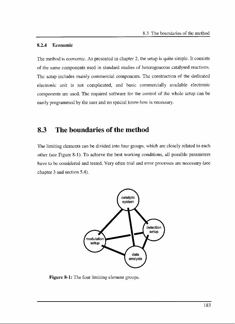
8.3 The boundaries of the method
8.2.4 Economic
The method is economic. As presented in chapter 2, the setup is quite simple. It consists
of the same components used in standard studies of heterogeneous catalysed reactions.
The setup includes mainly commercial components. The construction of the dedicated
electronic unit is not complicated, and basic commercially available electronic
components are used. The required software for the control of the whole setup can be
easily programmed by the user and no special know-how is necessary.
8.3 The boundaries of the method
The limiting elements can be divided into four groups, which are closely related to each
other (see Figure 8-1). To achieve the best working conditions, all possible parameters
have to be considered and tested. Very often trial and error processes are necessary (see
chapter 3 and section 5.4).
Figure 8-1: The four limiting element groups.
183
8. Conclusions
8.3.1 The detection setup
FTIR spectrometers are flexible and powerful instruments, but have several limitations.
The Signal-to-Noise Ratio (SNR) of the obtained spectra depends on the number of
photons per time reaching the detector (ADC-Counts). A large ADC-Counts number
produces a high SNR signal and therefore spectra of high quality.
There are several ways to ensure a sufficient SNR. A high intensity IR source or a better
detector can be used. A larger aperture is another possibility, but this can limit the
observable range of the electromagnetic spectrum. The lowpass filtering of the collected
signal can be eliminated, but the additional noise is added to the spectrum. Other
solutions are an increase in the number of collected scans per spectrum or the reduction
of the detector velocity. Both of these parameters are closely related to the time
resolution.
8.3.2 The analysis of the data
The time resolution of the FTIR determines the shortest detectable modulation period,
because a minimal number of points per period have to be measured, to fit the
sinusoidal curve. By reducing the modulation frequency the resolution of the retardation
is also reduced.
The collected data are analysed using an appropriate model. The choice of the model is
very important. It has to be simple, because a large number of degrees of freedom gives
rise to parameter values with large errors, artefacts and unrealistic results.
Additionally, the used gas flow can influence the resolution of the phase shift. The
induced effects depend on the reaction step. A reaction step taking place on the surface
is not influenced by the total gas flow. A reaction step involving gas phase species, e. g.
an adsorption/desorption process, results in a better resolved phase shift with a smaller
184
8.3 The boundaries of the method
gas flow, because the residence time x is larger, and x defines the highest possible time
retardation.
To develop a good model it is necessary to monitor the largest accessible number of
intermediates and products. Due to the attenuation of the intensity of the modulated
signal component along the reaction pathway, the largest possible amplitude of the
perturbation signal must be applied.
8.3.3 The modulation setup
The generation of the desired perturbation pattern is limited in frequency and amplitude.
The reaction and adjustment times of the used mass flow controller (MFC), together
with the chosen amplitude, limit the applicable frequency. An excessively high
modulation frequency, or a too large amplitude prohibits the correct implementation of
the desired feed gas composition, because changes in the setpoints are faster than the
adjustment of the output.
The amplitude is limited by the minimum and maximum flow of the MFC. The use of a
wide range MFC can not really help, because the regulation of reduced flows or small
amplitudes is very unprecise due to the sensitivity of the instrument. Preferable hence is
the use of pre-mixed gases with different reactant-to-inert gases ratio.
The used concentrations should be high for detection, but below the saturation of the
detector or the surface of the catalyst.
8.3.4 The catalytic system
The investigated catalytic system requires detailed consideration. Experimental
conditions must be chosen away from regimes, which causes unwanted effects. The
185
8. Conclusions
used catalyst has to react to the induced perturbations and produce a response signal.
The concentration change of the surface species on the catalyst induces a modification
of the reflectivity of the sample, which can strongly affect the SNR of the spectra. From
this point of view a small change of the concentrations in the feed gas is preferred,
because the induced modification of the reflectivity is limited.
8.4 Outlook
The method can be improved in several ways.
8.4.1 Better detection
The experimental setup can be improved by using a synchrotron IR beam as source,
which has a higher intensity within a well defined emission range compared to a
common SiC globar source (with Boltzmann distribution of a black-body emission).
Advantages are: an expected large improvement of the SNR, resulting in an
improvement of the time resolution (lower number of necessary scans); better detection
limits, allowing measurements of smaller concentrations. It is also possible to perform
experiments with a large IR beam without limitations in the range of the
electromagnetic spectrum.
An estimation of the possible improvements, which can be achieved by a synchrotron
source, is given below, using data from test measurements of KBr in the DRIFT cell. In
the best case (CO oxidation) with an aperture of 3.5 mm and collecting 64 scans (4.16 s)
per spectrum, a mean value for the SNR of 500 was achieved. Collecting a minimal
number of 5 to 6 spectra per modulation period, gives a lower limit of 25 s per period. If
a 1000 times more intense source (e. g. synchrotron) is used, the same SNR could
186
8.4 Outlook
theoretically be achieved by collecting only one scan (0.065 s) with an aperture of 0.3
mm diameter.
8.4.2 Faster measurements
The test experiments necessary to establish the optimum experimental conditions are a
time consuming process. To save time, a standard method for the test measurements
must be established. Test patterns different from step up/step down can be considered.
The data resolution to obtain phase shift can be improved by collecting spectra over
several modulation periods, calculating the desired integral values, combining together
the obtained values, and performing a Fast Fourier Transform (FFT). In a single step,
frequency and retardation are obtained.
Another way to reduce the measurement time is the application of perturbation patterns
which are generated by the combination of sinusoidal curves of different frequencies.
However, due to the non linear relation between concentration and IR intensity ghost
frequencies can be obtained in the fitting routine. Therefore, it is important to choose an
adequate fitting algorithm.
Additional errors due to changes in the optical reflectivity should be also considered.
8.4.3 Improved experiments
To elucidate complex catalytic systems, it is possible to use specific precursors to obtain
adsorbed intermediate compounds, which are expected to be involved in the reaction.
This would allow to bypass difficult steps and to derive more details about the
investigated system. The modulation setup can be improved to allow the introduction of
calibrated amounts of sublimated compounds, which would expand the above
possibilities described.
187
8. Conclusions
The development of the necessary models is not trivial, therefore, simplest model should
be chosen.
8.4.4 Additional investigations
The creation of a data base of systems in heterogeneous catalysis which have been
successfully investigated by the modulation technique would be most helpful.
Preliminary test experiments as well as complete studies using a variety of catalysts
would be useful. At the moment there is no way to asses a priori which catalysts are
suitable for these experiments.
The concept of modulation technique can also be applied to investigations in the
homogeneous catalysis and in material exchange processes. The relationships between
retardations and process parameters can be obtained analogously as explained in chapter
3.
8.5 Final remarks
The modulation technique expands the range of application of FTIR and DRIFT
spectroscopy in heterogeneous catalysis. It is noteworthy that it is possible to collect
data and to perform quantitative measurements without calibration curves or ad hoc
mathematical models for calibration.
This method is a powerful tool, which can still be improved in the future. In this work,
the basis of the modulation theory, as well as several examples of applications have
been reported. Further implementations and investigations of other catalytic systems are
necessary to fully exploit the potential of this technique.
188
Curriculum vitae
Curriculum vitae
Personal
Enrico Eugenio Ortelli, from Meride (TI), single, born December 3, 1971 in Lugano,
Switzerland.
Education
Sept.'77 - June '82 : Primary School in Lugano
Sept.'82 - June '86 : Secondary School in Lugano
Sept.'86-June'91 : Scientific College in Lugano
GCE-A level: Scientific including English
Major Topics: Computer science
Electronics
Nov.'91 - April '96 : Swiss Federal Institute of Technology (ETH) in Zürich,
Diploma in Chemical Engineering. Advisor: Prof. Dr. A. Baiker.
Major Topics: Biological Reaction Techniques
Layout and Computation of Technical Equipment
Analytical Methods of Technical Chemistry
June '96 - May '00 : Ph.D. thesis at the Swiss Federal Institute of Technology (ETH)
in Zürich, with experimental work carried out at the Paul
Scherrer Institut in Villigen. Advisor: Prof. Dr. A. Wokaun
189
Curriculum vitae
Referred Publications
Publications in preparation, and submitted are not listed.
D. Franzke, J. Kritzenberger, E. E. Ortelli, A. Baindl, O. Nuyken and A. Wokaun,
"Photolysis and thermolysis of diaryl(pentazadiene) compounds in solid matrix
investigated by infrared spectroscopy", /. Photochem. Photobiol. A: Chem. 112 (1998),
63-72.
E. E. Ortelli, J. M. Weigel and A. Wokaun, "Methanol synthesis pathway over Cu/Zr02
catalysts: a time-resolved DRIFT 13C-labelling experiment", Catal. Lett. 54 (1998), 41-
48.
E. E. Ortelli and A. Wokaun, "Use of periodic variations of reactant concentrations in
time resolved FTIR studies of heterogeneously catalysed reactions", Vib. Spectrosc. 19
(1999), 451-459.
M. A. Reiche, E. Ortelli and A. Baiker, "Vanadia grafted on Ti02-Si02, Ti02 and Si02
aerogels Structural properties and catalytic behaviour in selective reduction of NO by
NH3", Appl. Catal. B: Environmental 23 (1999), 187-203.
E. E. Ortelli, J. Wambach, A. Wokaun, "Use of periodic variations of reactant
concentrations in time resolved DRITT studies of heterogeneously catalysed reactions",
App. Catal. A: General 192 (2000), 137-152.
T. Lippert, E. Ortelli, J.-C. Panitz, F. Raimondi, J. Wambach, J. Wei and A. Wokaun,
"Imaging-XPS/Raman Investigation on the Carbonization of Polyimide after Irradiation
at 308 nm", Appl. Phys. A69 (1999), 651-654.
E. E. Ortelli, F. Geiger, T: Lippert, J. Wei and A. Wokaun, "UV-Laser Induced
Decomposition of Kapton Studied by Infrared Spectroscopy",Macromolecules, in print.
190
Curriculum vitae
Other publications
E. E. Ortelli and A. Wokaun, "Evidence of intermediates in methanol synthesis over
Cu/Zr02 catalysts: A time resolved, 13C-labelled experiment in DRIFT", PSI Annual
Report, Annex V, Villigen, 1998.
E. E. Ortelli and A. Wokaun, "Use of periodic variations of reactant concentrations in
time resolved FTIR studies of CO oxidation on Pd/Zr02 catalysts", PSI Annual Report,
Volume V, Villigen, 1999.
E. E. Ortelli, J. M. Wambach and A. Wokaun, "Determination of kinetical Data: a novel
application of DRIFT Modulation spectroscopy", PSI Annual Report, Volume V,
Villigen, 2000.
Posters
E. E. Ortelli and A. Wokaun, "Use of Periodic Variations of the Reactant
Concentrations in Time Resolved FTIR Studies of Heterogeneous Catalyzed Reactions",
AIRS III, Wien, July 5-8, 1998.
T. Lippert, E. Ortelli, J.-C. Panitz, F. Raimondi, J. Wambach, J. Wei and A. Wokaun,
"Imaging-XPS/Raman Investigation on the Carbonization of Polyimide after Irradiation
at 308 nm", COLA'99, Göttingen, July 19-23, 1999.
J. A. Anna Selvan, D. Grützmacher, E. Müller, E. Ortelli, A. Wokaun, H. Sigg, S. Stutz
and J. Gobrecht "Building Blocks for the Development of Thin Film Si Solar Cells",
National Photovoltaic Conference '99, Zürich, November 10-11, 1999.
191

Curriculum vitae
Talks
E. E. Ortelli and A. Wokaun, "Periodic Vanations of the Reactant Concentrations in
Time Resolved FTIR Studies of Heterogeneously Catalysed Reactions", CERC3,
Helsinki, May 20-23, 1999.
192
Bibliography
Bibliography
[I] J. Weidlein, U. Müller and K. Dehnicke, Schwingungsspektroskopie,G. Thieme Verlag, Stuttgart, New York, 1982.
[2] H.-H. Perkampus, Spektroskopie, VCH, Weinheim, New York, Basel,
Cambridge, 1993.
[3] A. A. Michelson, in Light Waves And Their Use, Univ. of Chicago Press, 1902.
[4] R. Bracewell, The Fourier Transform and Its Applications, McGraw-Hill,
New York, 1965.
[5] A. Papoulis, The Fourier Integral and Its Applications, McGraw-Hill,New York, 1962.
[6] P. B. Fellgett, /. Phy. Radium, 19 (1958), 237.
[7] P. Jacquinot, Rep. Prog. Phys. 13 (1960), 267.
[8] J. W. Cooley and J. W. Tuckey, Math. Comput. 19 (1965), 297.
[9] J. Connes and P. Connes, /. Opt. Soc. Am. 56, (1966), 896.
[10] R. P. McDonald and P. A. Wilks, Appl. Spectrosc. Al (1988), 151.
[II] P. R. Griffiths and J. A. de Haseth, Fourier Transform Infrared Spectrometry,vol. 83 of Chemical Analysis: A Series ofMonographs on Analtical Chemistryand Its Applications, J. Wiley & Sons, New York, 1986.
[12] J. R. Ferraro and K. Krishnan, Practical Fourier Transform Infrared
Spectroscopy, Academic Press, San Diego, 1990.
[13] P. Kubelka and F. Munk, Z. Tech. Phys. 12 (1931), 593.
193
Bibliography
[14] P. Kubelka, /. Opt. Soc. Am. 38(5) (1948), 1067.
[15] P. Kubelka, /. Opt. Soc. Am. 44 (1954), 330.
[16] G. Kortum, Spectrochim. Acta 6 (1957), 534.
[17] G. Kortum, Trans. Faraday Soc. 58 (1962), 1624.
[18] G. Kortum, W. Braun and G. Herzog, Angew. Chem. Intern. Ed. 2 (1963), 333.
[19] N. T. Melamed, /. Appl. Phys. 34(3) (1963), 560.
[20] P. D. Johnson, /. Appl. Phys. 35(2) (1964), 334.
[21] W. W. Wendlandt and H. G. Hecht, in Reflectance Spectroscopy, Interscience
Publishers, New York, London, 1966.
[22] W. K. Van Every and P. R. Griffiths, Appl. Spectrosc. 45(3) (1991), 347.
[23] E. M. Suzuki and W. R. Gresham, /. For. Sei. 31 (1986), 931.
[24] M. T. McKenzie and J. L. Koenig, Appl. Spectrosc. 39(3) (1985), 408.
[25] R. G. Messerschmidt, Appl. Spectrosc. 39(4), (1985), 737.
[26] R. Marbach and H. M. Hesse, in 8* International Conference on Fourier
Transform Spectroscopy, 288-289, H. M. Heise, E. H. Korte and H. W. Siesler,
1575 SPIE, 1991.
[27] D. J. J. Fraser and P. R. Griffiths, Appl. Spectrosc. 44(2) (1990), 193.
[28] M. Milosevic, Mikrochim. Acta, II (1988), 137.
[29] M. L. E. TeVrucht and P. R. Griffiths, Appl. Spectrosc. 43(8) (1989), 1492.
[30] S. A. Yeboah, S.-H. Wang and P. R. Griffths, Appl. Spectrosc. 38(2) (1984),259.
[31] Z. Krivâcsy and J. Hlavay, J. Spec. Acta, 50A(1) (1994), 49.
194
Bibliography
[32] K. Moradi, C. Depecker and J. Corset, Appl. Spectrosc. 48(12) (1994), 1491.
[33] A. A. Christy, Y. Liang, C. Hui, O. M. Kvalheim and R. A. Velapoldi, Vib.
Spectrosc. 5 (1993), 233.
[34] N. E. Sharpless and D. A. Gregory, Appl. Spectrosc. 17 (1962), 47.
[35] R. K. Vincent and G. R. Hunt, Appl. Opt. 7 (1968), 7.
[36] K. Moradi, C. Depecker, J. Barbillat and J. Corset, Spectrochimica Acta A: Mol
and Biomol. Spectrosc. 55(1) (1999), 43.
[37] IM. Hamadeh, S. A. Yeboah, K.A.Trumbull and P.R.Griffiths, Appl.
Spectrosc. 38(4) (1984), 486.
[38] F. Boroumand, J. E. Moser and H. Van den Bergh, Appl. Spectrosc. 46(12)
(1992), 1874.
[39] D. Reinecke, A. Jansen, F. Fister and U. Schernau, Anal. Chem. 60 (1988),1221.
[40] R. S. S. Murthy and D. E. Leyden, Anal. Chem. 58 (1986), 1228.
[41] J. M. Chalmers and M. W. MacKenzie, in Advances in Applied Fourier
Transform Infrared Spectroscopy, J. Wiley & Sons, Chichester, 1988.
[42] R. W. Frei, D. E. Ryan and V. T. Lieu, Canadian J Chem. 44 (1966), 1945.
[43] E. L. Simmons, Appl. Opt. 14(6) (1975), 1380.
[44] H. G. Hecht, Anal. Chem. 48(12) (1976), 1775.
[45] T. Hattori, K. Shirai, M. Niwa and Y. Murakami, Bull. Chem. Soc. Jpn. 54
(1981), 1964.
[46] A. A. Christy, O. M. Kvalheim and R. V. Velapoldi, Vib. Spectrosc. 9 (1995),
19.
[47] S. K. Loyalka and C. A. Riggs, Appl. Spectrosc. 49(8) (1995), 1107.
195
Bibliography
[48] B. Azambre, O. Heintz, M. Schneider, A. Krzton and J. V. Weber, Talanta,
50(2) (1999), 359.
[49] K. Tamaru, Adv. Catal. 15 (1964), 65.
[50] M. Kobayaski and K. Kobayaski, Catal. Rev.-Sci. Eng. 10 (1974), 139.
[51] C. O. Bennett, Ibid. 15 (976), 121.
[52] S. F. Parker, A. Amorelli, Y. D. Amos,C. Hughes, N. Porter and J. R. Walton,
J. Chem. Soc. Faraday Trans. 43(91) (1995), 517.
[53] W. W. Coblentz, J. Franklin Inst. 172 (1911), 309.
[54] M. P. Fuller and P. R. Griffiths, Anal. Chem. 50 (1978), 1906.
[55] M. P. Fuller and P. R. Griffiths, Amer. Lab. 10 (1978), 69.
[56] M. P. Fuller and P. R. Griffiths, Appl. Spectrosc. 34(5) (1980), 533.
[57] LabVIEW, Tutorial, National Instruments.
[58] Troutmann, 5f programming postulate, in Murphy's Law, A. Bloch, Methuen,
London, 1985.
[59] Mass Flow Controller, Operating Manual, Bronkhorst.
[60] Liqui Flow, Operating Manual, Bronkhorst.
[61] Controlled Evaporator Mixer, Operating Manual, Bronkhorst.
[62] T-Control 94C, Operating Manual, Eurotherm.
[63] T-Control 847, Operating Manual, Eurotherm.
[64] T-Control 904A, Operating Manual, Eurotherm.
[65] Model 0030-100, Operating Manual, Spectra Tech.
[66] Model 0030-0XX, Operating Manual, Spectra Tech.
196
Bibliography
[67]'
Environmental Chamber 19930, Operating Manual, Grasby-Specac.
[68] Selector Diffuse Reflectance Accessory 19900, Operating Manual,
Grasby-Specac.
[69] M. R. Praire, A. Renken, J. G. Highfield, K. R. Thampi and M. Grätzel, /.
Catal. 129 (1991), 130.
[70] J. M. Olinger and P. R. Griffiths, Anal. Chem. 60 (1988), 2427.
[71] N. R. Smyrl, E. L. Fuller Jr. and G. L. Powell, Appl. Spectrosc. 37(1) (1983),39.
[72] C. Schild, A. Wokaun and A. Baiker, /. Mol. Cat. 63 (1990), 243.
[73] J. M. Weigel, Ph. D. thesis, ETH, Zürich, 1996.
[74] OPUS/IR, Operating Manual, Bruker GmbH.
[75] H. J. Güntherodt, in Rapidly Quenched Metals, vol. 2, 1591, S. Steeb &
H. Warlimont, Elsevier, Amsterdam, 1985.
[76] C. Fröhlich, R. A. Koppel, A. Baiker, M. Kilo and A. Wokaun, Appl. Cat. A:
General, 106 (1993), 275.
[77] R. A. Koppel, A. Baiker, Ch. Schild and A. Wokaun, Stud. Surf. Sei. Catal. 63
(1991), 59.
[78] R. B. Andersos and P. T. Dawson, Experimental Methods in CatalyticResearch, vol. 1, Academic Press, New York, 1968.
[79] R. B. Andersos and P. T. Dawson, Experimental Methods in CatalyticResearch, vol. 2, Academic Press, New York, 1976.
[80] R. B. Andersos and P. T. Dawson, Experimental Methods in CatalyticResearch, vol. 3, Academic Press, New York, 1976.
[81] H. Unbehauen, Regelungstechnik I, Vieweg, Braunschweig/Wiesbaden, 1992.
[82] H. Unbehauen, Regelungstechnik II, Vieweg, Braunschweig/Wiesbaden, 1992.
197
Bibliography
[83] H. Unbehauen, Regelungstechnik III, Vieweg, Braunschweig/Wiesbaden, 1992.
[84] J. Baillieul and J. C. Willems, Mathematical Control Theory, Springer Verlag,New York, 1999.
[85] A. Cichocki and R. Unbehauen, Neural Networks for Optimisation and Signal
processing, J. Wiley & Sons, Stuttgart, 1993.
[86] K. J. Aström and B. Wittenmark, Adaptive Control, Addison-Wesley, 1995.
[87] W. P. Aue, E. Bartholdi, R. R. Ernst, J.Chem.Phys. 64 (1976), 229.
[88] A. Bax, Two dimensional Nuclear Magnetic Resonance in Liquids, Reidel,
Boston, 1982
[89] D. L. Turner, Prog. Nucl. Magn. Reson. Spectrosc. 17 (1985), 281.
[90] R. R. Ernst, G. Bodenhausen, A. Wokaun, Principles of nuclear magneticresonance in one and two dimensions, Clarendon Press, Oxford, 1987.
[91] I. Noda, /. Am. Chem. Soc. 111(21) (1989), 8116.
[92] I. Noda, Appl. Spectrosc. 44(4) (1990), 550.
[93] I. Noda, A. E. Dowrey and C. Marcott, Appl. Spectrosc. 47(9) (1993), 1317.
[94] I. Noda, Appl. Spectrosc. 47(9) (1993), 1329.
[95] I. Noda, Y. Liu, Y. Ozaki and M. Czarnecki, J. Phys. Chem. 99(10) (1995),3068.
[96] H. Kobayashi and M. Kobayashi, Cat. Rev.-Sci. Eng. 10(2) (1974), 391.
[97] J. L. Falconer and J. A. Schwarz, catal. Rev.sci.eng. 25(2) (1983), 141.
[98] A. Baiker, Int. Chem. Ing. 25(1) (1985), 30.
[99] J. R. Schrieffer and J. H. Sinfelt, /. Phys. Chem. 94 (1990), 1047.
[100] H.-S. Liu, S.-C. Wu and S.-C. Lin, Chem. Eng. Comm. 164 (1998), 13.
198
Bibliography
[101] A. E. Rodrigues and M. M. Dias, Chem. Eng. Process. 37 (1998), 498.
[102] U. Fringeli, Simultaneous Phase-Sensitive Digital Detection process For Time-
Resolved Quasi Simultaneously Captured Data Arrays Of A PeriodicallyStimulated System, PCT/CH96/00293, WO 97/08598.
[103] I. S. Park, M. Petkovska and D. D. Do, Chem. Eng. Sei. 53(4) (1998), 819.
[104] I. S. Park, M. Petkovska and D. D. Do, Chem. Eng. Sei. 53(4) (1998), 833.
[105] G. Marcelin, J. E. Lester and S. Mitchell, J. Catal. 102 (1986), 240.
[106] J. Kritzenberger and A. Wokaun, /. Mol Catal. A: Chem. 118 (1997). 235.
[107] M. Cavers, J.M.Davidson, I. R. Harkness, G. S. McDougall and
L. V. C. Rees, Stud. Surf. Sei. Catal. 122 (1999), 65.
[108] J. G. Ziegler and N. B. Nichols, Trans. ASME, 64 (1942), 759.
[109] R. E. Murphy and H. Sakai, in Aspen International Conference on Fourier
Spectroscopy, G. A. Vanasse, A. T. Stair and D. Baker, Air Force Geophysics
Laboratory, Cambridge, 1971, 301.
[110] R. E. Murphy, F. Cook and H. Sakai, /. Opt. Soc. Am. 65 (1975), 600.
[Ill] R. A. Cracombes, A. A. Garrison and G. Mamantov, 9th International
Conference on Fourier Transform Infrared Spectroscopy, H. Sakai, Proc. Soc.
Photo-Opt. Instrum. Eng. 289 (1981), 36.
[112] G. Durry, G. Guelachvili, D.Mathieu and A. Ubelmann, 9th International
Conference on Fourier Transform Infrared Spectroscopy, J. H. Bertie and
H. Weiser, Proc. Soc. Photo-Opt. Instrum. Eng. 289 (1993), 110.
[113] G. Durry and G. Guelachvili, Appl. Opt. 34(12) (1995), 1971.
[114] J. M. Presses, G. E. Hall, J. T. Muckermann, T. J. Sears, E. Weston, G. Guyot,J. C. Hanson, G. W. Flynn and H. Bernstein, Rev. Sei. Instrum. 64 (1993), 95.
[115] J. F. Durana and A. W. Mantz, Fourier Transform Spectroscopy, vol.2,J. Ferraro and L. Basile, Academic, San Diego, 1979.
199
Bibliography
[116] J. J. Sloan, 7 International Conference on Fourier Transform Spectroscopy,D. G. Cameron, Proc. Soc. Photo-Opt. Instrum. Eng. 145 (1989), 10.
[117] H. Sakai and R. E. Murphy, Appl. Opt. 17 (1978), 1343.
[118] R. A. Palmer, J. L. Chao, R. M. Dittmar, V. G. Gregoriou and S. E. Plunkett,
Appl. Spectrosc. 47 (1993), 1297.
[119] B. O. Budevska and C. J. Manning, Appl. Spectrosc. 50(7) (1996), 939.
[120] R. A. Palmer, E. Y. Jiang and J. L. Chao, Mikrochim. Acta, Suppl. 14 (1997),591.
[121] S. V. Shilov, H. Skupin, F. Kremer, E. Gebhard and R. Zentel, Liq. Cryst.
22(2) (1997), 203.
[122] R. A. Palmer, G. D. Smith and P. Y. Chen, Vib. Spectrosc. 19(1) (1999), 131.
[123] O. Levenspiel, Chemical Reaction Engineering, J. Wiley & Sons, international
edition, 1972.
[124] M. Baerns, H. Hoffmann and A. Renken, Chemische Reaktionstechnik,
G. Thieme Verlag, Stuttgart, New York, 1987.
[125] E. E. Ortelli and A. Wokaun, Vib. Spectrosc. 19 (1999), 451.
[126] A. Bill, Ph. D. thesis, EPF, Lausanne, 1998.
[127] M. Bowker, H. Houghton and K. Waugh, J. Chem. Soc. Faraday Trans. 77
(1981), 3023.
[128] G. Chinchen, P. Denny, J. Jennings, M. Spencer and K. Waugh, Appl. Catal.
36(1988), 1.
[129] M. Muhler, L. P. Nielsen, E. Törnqvist, B. S. Clausen and H. Tops0e, Catal.
Lett. 14 (1992), 241.
[130] B. Denise and R. Sneeden, Appl. Catal. 28 (1986), 235-239.
200
Bibliography
[131] C.V. Ovesen, P. Stoltze, J. K. N0rskov and C.T.Campbell, /. Catal. 134
(1992), 445
[132] C. V. Ovesen, B. S. Clausen, B. S. Hammersh0i, G. Steffensen, T. Askgaard,I. Chorkendorff, J. K. N0rskov, P. B. Rasmussen, P. Stoltze and P. Taylor, J.
Catal. 158 (1996), 170.
[133] C. V. Ovesen, B. S. Clausen, J. Schi0tz, P. Stoltze, H. Tops0e and
J. K. N0rskov, /. Catal. 168(2) (1997), 133.
[134] T. S. Askgaard, J. K. N0rskov, C. V. Ovesen and P. Stoltze, /. Catal. 156
(1995), 229.
[135] E. E. Ortelli, J. Wambach and A. Wokaun, Appl. Catal. 192(1) (2000), 137.
[136] D. Böcker and E. Wicke, Ber. Bunsenges. Phys. Chem. 89 (1985), 629.
[137] B. C. Sales, J. E. Turner and M. B. Maple, Surf. Sei. 114 (1982), 381.
[138] T. Engel and G. Ertl, Advan. Catal. 28 (1979), 1.
[139] H. Conrad, G. Ertl, and J. Küppers, Surf. Sei. 76 (1978), 33.
[140] T. Engel and G. Ertl, J. Chem. Phys. 69 (1978), 1267.
[141] T. Engel, /. Chem. Phys. 69 (1978), 373.
[142] S. Ladas, R. Imbihl and G. Ertl, Surf. Sei. 219 (1989), 88.
[143] Y. Q. Deng, T. G. Nevell and M. G. Jones, Catal. Lett. 34 (1995), 313.
[144] T. loannides, A. M. Efstathiou, Z. L. Zhang and X. E. Verykios, J. Catal. 156
(1995), 265.
[145] Yu. Suchorski, J. Beben and R. Imbihl, Surf. Sei. 405 (1998), L477.
[146] R. L. Keiski, M. Härkönen, A. Lathi, T. Maunula, A. Savimäki and T. Slotte, in
Proceedings CAPoC3 Conference, Brussels, 1994, 53.
[147] A. Baiker, D. Gasser, J. Lenzner, /. Chem. Soc. Chem. Commun. (1987), 1750.
201
Bibliography
[148] A. Baiker, Faraday Discuss. Chem. Soc. 87 (1987), 239.
[149] A. Baiker, D. Gasser, J. Lenzner, A. Relier and S. Schlögl, /. Catal. 126
(1990), 555.
[150] A. Baiker, M. Maciejewski and S. Tagliaferri, Ber. Bunenges. Phys. Chem. 91
(1993), 3.
[151] P. Barnickel, A. Wokaun and A. Baiker, /. Chem. Soc. Faraday Trans. 87(2)
(1991), 333.
[152] L. M. Sander and S. V. Ghaisas, Surf. Sei. 391 (1997), 125.
[153] H. J. Güntherodt, Rapidly Quenched Metals, vol. 2, S. Steeb & H. Warlimont,
Elsevier, Amsterdam, 1985, 1591.
[154] T. Nijhuis, M. Makkee, A. Van Langeveld and J. Moulijn, Appl. Catal. A:
General 164 (1997), 237.
[155] E. E. Ortelli, J. M. Weigel and A. Wokaun, Catal. Lett. 54 (1998), 41.
[156] M.-Y. He and J. G. Ekerdt, /. Catal. 87 (1984), 238.
[157] M.-Y. He, J. M. White and J. G. Ekerdt, /. Mol. Catal. 30 (1985), 415.
[158] H. Abe, K. Maruya, K. Domen and T. Onishi, Chem. Lett. (1984), 1875.
[159] Y. Amenomiya, Appl. Catal. 30 (1987), 57.
[160] Y. Sun and P. A. Sermon, J. Chem. Soc, Chem. Commun. (1993), 1242.
[161] C. Schild, A. Wokaun and A. Baiker, /. Mol. Cat. 63 (1990), 223.
[162] C. Schild, A. Wokaun and A. Baiker, Fres. J. Anal. Chem. 341 (1991), 395.
[163] R. A. Koppel, A. Baiker, C. Schild and A. Wokaun, J. Chem. Soc, FaradayTrans. 87(17) (1991), 2821.
[164] A. Wokaun, J. M. Weigel, M. Kilo and A. Baiker, Fres. J. Anal. Chem. 349
(1994), 71.
202
Bibliography
[165] J. M. Weigel, C. Fröhlich, A. Baiker and A. Wokaun, Appl. Catal. 140 (1996),29.
[166] I. Fisher, H.-C. Woo and A. Bell, Catal. Lett. 44 (1997), 11.
[167] I. Fisher and A. Bell, /. Catal. 172 (1997), 222.
[168] C. Fröhlich, R. A. Koppel, A. Baiker, M. Kilo and A. Wokaun, Appl. Cat. A:
General 106 (1993), 275.
[169] G. J. Millar, C. H. Rochester and K. C. Waugh, /. Chem. Soc, Faraday Trans.
88(15) (1992), 2257.
[170] A.B.Anton, J. E. Parmeter and W.H.Weinberg, /. Am. Chem. Soc 107
(1985), 5558.
[171] K. Weissermel and H.-J. Arpe, Industrielle Organische Chemie: Bedeutende
Vor- und Zwischenprodukte, VCH, Weinheim, 1994.
[172] M. Bowker, R. A. Hadden, H. Houghton, J. N. K. Hyland and K. C. Waugh, J.
Catal. 109 (1988), 263.
[173] E. Ramroson, R. Kieffer and A. Kiennemann, Appl. Catal. 4 (1982) 281.
[174] J. F. Edwards and G. L. Schrader, J. Catal. 94 (1985), 175.
[175] A. Kiennemann, H. Idriss, J. Hindermann, J. Lavalley, A. Vallet, P. Chaumette
andP. Courty, Appl. Catal. 59 (1990) 165.
[176] R. J. Klinger and J. W. Rathke, J. Am. Soc. 106 (1984), 7650.
[177] J. F. Edwards and G. L. Schrader, /. Phys. Chem. 88 (1984), 5620.
[178] A. Ueno, T. Onishi and K. Tamaru, /. Catal. 66 (1970), 756.
[179] M. Bowker, H. Hougton and K. C. Waugh, J. Chem. Soc, Faraday Trans. 11
(1981)3023.
[180] M. Bowker, H. Hougton, K. C. Waugh, T. Giddings and M. Green, J. Catal. 84
(1983) 252.
203
Bibliography
[181] M. Bowker, Vacuum 33 (1983), 669.
[182] S. G. Neophytides, A. J. Marchi and G. F. Froment, Appl. Cat. A: General 86
(1992), 45.
[183] G.C. Chinchen, P. J. Denny, J. R. Jennings, M. S. Spencer and D. A. Whan,
Appl. Catal A 30 (1987), 333.
[184] P. B. Rasmussen, M. Kazuta and I. Chorkendorff, Surf. Sei. 318 (1994), 267.
[185] J. Weigel, R. Koppel, A. Baiker and A. Wokaun, Langmuir 12(22) (1996),5319.
[186] M. Kilo, J. Weigel, A. Wokaun, R. A. Koppel and A. Baiker, J. Mol. Catal. A
Chem. 126(2-3) (1997), 169.
[187] J. Wambach, A. Baiker and A. Wokaun, Phys. Chem. Chem. Phys. 1 (1999),5071.
[188] S.Bailey, G. F. Froment, J. W. Snoeck and K. C. Waugh, Catal. Lett. 30
(1995), 99.
[189] S. Wohlrab, D. Ehrlich, J. Wambach, H. Kuhlenbeck and H.-J. Freund, Surf.Sei. 220 (1989), 243.
[190] C. Binet, A. Badri, M. Boutonnet-Kizling and J.-C. Lavalley, /. Chem. Soc,
Faraday Trans. 90(7) (1994), 1023
[191] J. Nerlov, S. Sckerl, J. Wambach and I. Chorkendorff, Appl. Catal. A: General
191 (2000), 97.
[192] J. H. Larsen and I. Chorkendorff, Surf. Sei. 405 (1998), 62.
[193] B. S. Clausen, J. Schi0tz, L. Grabaek, C. V. Ovesen, K. W. Jacobsen,J. K. Norskov andH. Tops0e, Top. Catal. 1 (1994), 367.
[194] H. Tops0e, C. V. Ovesen, B. S. Clausen, N.-Y. Tops0e, P. E. Hojlund Nielsen,E. Törnqvist and J. K. Norskov, Dynamics ofSurfaces and Reaction Kinetics in
Heterogeneous Catalysis, G. F. Froment and K. C. Waugh, Elsevier,
Amsterdam, 1997.
204
Bibliography
[195] N.-Y. Tops0e and H. Tops0e, /. Mol. Catal. A: Chem. 141 (1999), 95.
[196] T. H. Fleisch and R. L. Mieville, J. Catal. 90 (1984), 165.
[197] B. S. Clausen, G. Steffensen, B. Fabius, J. Villadsen, R. Feidenhans'l and
H. Tops0e, /. Catal. 132 (1991), 524.
[198] K. Waugh, Catal. Today 15 (1992), 51.
[199] M. E. Bridge, C. M. Comrie and R. M. Lambert, Surf. Sei. 67 (1977), 393
[200] F. Falo, I. Cano and M.Salmerön, Surf. Sei. 143 (1984), 303.
[201] M. T. Paffett, C. T. Campbell, T. N. Naylor and S. Srinivasan, Surf. Sei. 154
(1985), 284.
[202] U. Schneider, G. R. Castro and K. Wandelt, Surf. Sei. 287/288 (1993), 146.
[203] A. Ruban, B. Hammer, P. Stoltze, H. L. Skriver and J. K. N0rskov, /. Mol.
Catal. A 115 (1997), 421.
[204] B. Hammer and J. K. N0rskov, Surf. Sei. 343(3) (1995), 211.
[205] B. Hammer, Y. Morikawa and J. K. N0rskov, Phys. Rev. Lett. 76 (1996), 2141.
[206] J. B. Hansen, Handbook ofHeterogeneoul Catalysis, G. Ertl, H. Knözinger and
J. Weitkamp, VCH, Weinheim, 1997.
[207] G. H. Graaf, P. J. J. M. Sijtsema, E. J. Stamhuis, G. E. H. Joosten, Chem. Eng.Sei. 41 (1986), 2883.
[208] R. A. Koppel, A. Baiker and A. Wokaun, Appl. Catal. A: General 84 (1992),77.
205


![[Charles N. Satterfield] Heterogeneous Catalysis](https://img.pdfslide.us/doc/110x75/577cc1a51a28aba71193945e/charles-n-satterfield-heterogeneous-catalysis.jpg)

![Heterogeneous Catalysis [Basic Concepts] - Jens Norskov](https://img.pdfslide.us/doc/110x75/542ac2c4219acd89798b472d/heterogeneous-catalysis-basic-concepts-jens-norskov.jpg)