Spectro-temporal factors in two-dimensional human sound ...johnvo/papers/jasa.pdf · Spectro-temporal factors in two-dimensional human sound localization Paul M. Hofmana) and A. John

Spectro-temporal factors in two-dimensional human soundlocalization

Paul M. Hofmana) and A. John Van OpstalUniversity of Nijmegen, Department of Medical Physics and Biophysics, Geert Grooteplein 21,6525 EZ Nijmegen, The Netherlands

~Received 6 June 1997; revised 5 December 1997; accepted 29 January 1998!

This paper describes the effect of spectro-temporal factors on human sound localizationperformance in two dimensions~2D!. Subjects responded with saccadic eye movements to acousticstimuli presented in the frontal hemisphere. Both the horizontal~azimuth! and vertical~elevation!stimulus location were varied randomly. Three types of stimuli were used, having differentspectro-temporal patterns, but identically shaped broadband averaged power spectra: noise bursts,frequency-modulated tones, and trains of short noise bursts. In all subjects, the elevationcomponents of the saccadic responses varied systematically with the different temporal parameters,whereas the azimuth response components remained equally accurate for all stimulus conditions.The data show that the auditory system does not calculate a final elevation estimate from along-term~order 100 ms! integration of sensory input. Instead, the results suggest that the auditorysystem may apply a ‘‘multiple-look’’ strategy in which the final estimate is calculated fromconsecutive short-term~order few ms! estimates. These findings are incorporated in a conceptualmodel that accounts for the data and proposes a scheme for the temporal processing of spectralsensory information into a dynamic estimate of sound elevation. ©1998 Acoustical Society ofAmerica.@S0001-4966~98!03005-7#

PACS numbers: 43.66.Qp, 43.66.Ba, 43.66.Mk@RHD#

u-u

oem

t lck

am

eanannannd

thed96aextu

ed-flo-

nnat,

ted-

ese

-

rys of

om

ro-iblep-the

um

INTRODUCTION

Human auditory localization depends on implicit binaral and monaural acoustic cues. Binaural cues arise throinteraural differences in sound level~ILD ! and timing~ITD!that relate in a simple way to the horizontal componentsound direction relative to the head. The auditory systhowever, cannot distinguish, from these cues, betweensource positions with the same horizontal component thaon the so-called ‘‘cone of confusion.’’ Due to the front–basymmetry of the ITD and ILD cues, a sound azimuth~a!estimate provided by these binaural cues is thereforebiguous~e.g., Blauert, 1996; Wightman and Kistler, 1992!.

Monaural cues consist of direction-dependent linspectral filtering caused by the torso, head, and pinnae. Ident waveforms are reflected and diffracted in a complexdirection-dependent way, which typically gives rise to stroenhancement and attenuation at particular frequency b~Hebrank and Wright, 1974; Shaw, 1974; Mehrgardt aMellert, 1977; Middlebrookset al., 1989; Lopez-Poveda anMeddis, 1996!. These cues are essential for elevation~e! lo-calization and in resolving front–back ambiguities~e.g., Bat-teau, 1967; Musicant and Butler, 1984; Blauert, 1996!.

The relation between the pinna geometry anddirection-dependent filtering has been shown in both expmental and theoretical studies~Batteau, 1967; Teranishi anShaw, 1968; Han, 1994; Lopez-Poveda and Meddis, 19!.The actual importance of the filtering in two-dimensionlocalization has been underlined by various behavioralperiments. In some of these studies, the geometrical struc

a!Electronic mail: [email protected]

2634 J. Acoust. Soc. Am. 103 (5), Pt. 1, May 1998 0001-4966/98/10

gh

f,

allie

-

rci-d

gdsd

eri-

l-re

of the pinna was altered artificially, resulting in a degradlocalization performance~Gardner and Gardner, 1973; Oldfield and Parker, 1984b!. In other studies, manipulation othe sound spectra and the resulting effects on elevationcalization could be related to spectral features in the pifilters ~e.g., Middlebrooks, 1992; Butler and Musican1993!.

The features in the spectral pinna filter, or head-relatransfer function~HRTF!, are believed to carry the information about sound location~Kistler and Wightman, 1992!.Yet, a fundamental problem arises in the processing of thfeatures into estimates of sound location~Zakarouskas andCynader, 1993; Hofman and Van Opstal, 1997!. At the levelof the eardrums, the available spectrum,y(v;rS), associatedwith the source position,rS5(aS ,eS), results from thesource spectrum,x(v), filtered by the particular directiondependent HRTF,h(v;rS):

y~v;rS!5h~v;rS!•x~v! ~1!

with v the frequency in octaves. In principle, the auditosystem has no knowledge about the relative contributionneitherh(v;rS) nor x(v). Yet, it is necessary to minimizethe source influences in order to recognizeh(v;rS) and thusdetermine the position,rS ~mainly elevation and front–backangle, as left–right angle is determined predominantly frbinaural cues!.

So far, only a few computational models have been pposed, which suggest how this could be done. A posssolution to this problem would be to make a priori assumtions about the sound source spectrum. It would enableauditory system to directly compare the incoming spectrto the ~stored! HRTFs ~e.g., Netiet al., 1992; Zakarouskas

26343(5)/2634/15/$10.00 © 1998 Acoustical Society of America

neth

ncis

ae-petude

ksFmtrupof

oa

oar

in

aedragh

owsasednn

e-a

peIt

as

sn

re

im

es

di-e inofria-eddandtro-the

letead-

rio-ion

re-

rvi-

andu-

nsein

au-

ex-ectsf thel-suche ofor

andAlld.

nd

m,omdB

red

or-stede

and Cynader, 1993; Middlebrooks, 1992!. Neti et al. ~1992!showed that a feed-forward neural network could be traito accurately extract the location of broadband noise onbasis of the spectral filter properties of the cat’s pinna. Sithe model was only trained with white noise, however, itnot clear how it withstands spectral variations.

Zakarouskas and Cynader~1993! proposed a model inwhich the comparison between the cochlear spectrumthe HRTFs is based on spectral derivatives of first and sond order~i.e., dy/dv, d2y/dv2!. For a sound source spectrum that is locally constant, or has a locally constant slothe model was shown to recognize essential spectral feaof the underlying HRTF~specifically relevant peaks annotches!, and thus correctly extract the direction of thsound.

In an alternative model, proposed by Middlebroo~1992!, the sensory spectrum is compared with the HRTby computing a spectral correlation coefficient. This schesuggested that localization is accurate if the source specis broadband and sufficiently flat, such that the sensory inmaintains maximal correlation with the underlying HRTFthe associated source position.

In the latter two models, accurate localization reliesspecific spectral constraints on the source spectrum. Thissumption is supported by recent experimental results. Onhand, the auditory system appears to tolerate random vtions within the broadband sound spectrum~e.g., Wightmanand Kistler, 1989!. On the other hand, if relative variationsthe source spectrum become too large, localization candisturbed dramatically~e.g., Middlebrooks, 1992!. It there-fore remains unclear what the actual spectral constraints

So far, the majority of localization studies have applistimuli with stationary spectral properties. Yet, natusounds possess a high degree of nonstationarity. Althouis commonly accepted that spectral shape cues play ansential role in elevation detection, it is as yet unknown hthe auditory system applies the spectral analysis to nontionary sensory information. In addition, due to the fundmental relation between the temporal and spectral domainsufficiently high spectral resolution requires a minimal timwindow over which the spectral estimation is integrateD f •DT5constant. The temporal and spectral resolutioneeded for adequate sound localization, however, arewell known.

One possibility is that the sensory information is intgrated over a time scale of order, say, 100 ms to obtainaverage spectrum on which a spectral~shape! analysis can beapplied. If true, sounds with the same average power strum on that time scale would be localized equally well:would allow a considerable amount of freedom for the phspectrum on that time scale.

An alternative possibility could be that the auditory sytem applies a ‘‘multiple-look’’ strategy, in which elevatioestimation is based on multiple, consecutive short-term~say,of order a few ms! spectral analyses of the ongoing sensoinformation. This latter scheme would imply that thspectral-temporal behavior of the stimulus on that short tscale is also important.

In the present study, we specifically focused on th

2635 J. Acoust. Soc. Am., Vol. 103, No. 5, Pt. 1, May 1998

dee

ndc-

,res

sem

ut

ns-

neia-

be

re.

lit

es-

ta--, a

:sot

n

c-

e

-

y

e

e

spectro-temporal aspects for sound localization in twomensions. To our knowledge, such data are not availablthe current literature. In two experiments, the sensitivitythe localization process to short-term spectro-temporal vations was of interest. Localization to frequency-modulattones~‘‘FM sweeps’’! and trains of short-duration broadbanbursts was measured. These stimuli had similar broadbaverage power spectra, but fundamentally different spectemporal behaviors. In a third experiment, we estimatedminimal time needed by the localization process to compelevation estimation. To that means, localization to broband noise of various durations~3–80 ms! was measured. Ina recent pilot study by Frens and Van Opstal~1995!, it wasshown that localization performance systematically deterates in elevation, but not in azimuth, when stimulus duratof broadband noise bursts is shorter than 10 ms.

Saccadic eye movements were used to quantify thesponse accuracy. It enabled accurate measurements~within 1deg! of a very early spatial percept~below 200 ms! forstimuli presented within the oculomotor range~35-deg ec-centricity range in all directions!. Subjects were tested undeentirely open-loop conditions, i.e., neither acoustic, norsual or verbal feedback was provided.

The results of our experiments show a consistentsystematic influence of spectro-temporal factors of the stimlus on the elevation component of the localization respoin all subjects tested. These findings will be discussedterms of a conceptual spectro-temporal model of humanditory localization in two dimensions.

I. METHODS

A. Subjects

Seven male subjects participated in the localizationperiments. Their ages ranged from 23 to 39 years. Subjwere employees and students of the department. Three osubjects~PH, JO, and JG! were experienced in sound locaization experiments, whereas the other subjects had noprevious experience and were kept naive as to the purposthis investigation. Inexperienced subjects were given onetwo practice sessions to get acquainted with the setuplocalization paradigm and to gain stable performance.subjects reported to have no hearing problems of any kin

B. Apparatus

Experiments were conducted in a completely dark asound-attenuated room with dimensions 33333 m. Thewalls, floor, and ceiling were covered with acoustic foathat effectively absorbed reflections above 500 Hz. The rohad an A-weighted ambient background noise level of 30SPL.

The orientation of the subject’s right eye was measuwith the scleral search coil technique~Collewijn et al., 1975;Frens and Van Opstal, 1995!. The oscillating magnetic fieldsthat are needed by this method were generated by twothogonal pairs of square 333 m coils, attached to the room’edges: one pair of coils on the left and right walls generaa horizontal magnetic field~30 kHz! and a second pair on thceiling and floor created a vertical magnetic field~40 kHz!.

2635P. M. Hofman and A. J. Van Opstal: Localization factors

-aiozeon-

da

es

g

thr

nicens

unto

iot

a

ex-dy

theiallye

ce-ve-bye-

C-vely.qui-e:

-

nd

au-Cby

terC,

of

ed

rhinalletrolset

rom

mly

s

tiathed

An acoustically transparent frontal hemisphere~consist-ing of a thin wire framework, covered with black silk cloth!with 85 red light-emitting diodes~LEDs! was used for cali-bration of the eye-coil measurements and for providingfixation light at the start of each localization trial. LED coordinates are defined in a two-dimensional polar coordinsystem with the origin at the straight-ahead gaze directTarget eccentricity,RP@0,35# deg, is measured as the gaangle with respect to the straight-ahead fixation positiwhereas target direction,fP@0,360# deg, is measured in relation to the horizontal meridian. For example,R50 ~for anyf! corresponds to ‘‘straight ahead,’’ andf50, 90, 180, and270 deg~for R.0! correspond to ‘‘right,’’ ‘‘up,’’ ‘‘left,’’and ‘‘down’’ positions, respectively. LEDs were mounteat a distance of 85 cm from the subject’s eye,directions f50,30,60,...,330 deg and at eccentricitiR50,2,5,9,14,20,27,35 deg.

Sound stimuli were delivered through a broad-ranlightweight speaker~Philips AD-44725! mounted on a two-link robot ~see Fig. 1!. The robot consisted of a base witwo nested L-shaped arms, each arm driven by a sepastepping motor~Berger Lahr VRDM5! with an angular reso-lution of 0.4 deg. It enabled rapid~within 2 s! and accuratepositioning of the speaker at practically any point on a frotal hemisphere with a radius of 90 cm, the center of whwas aligned with the LED hemisphere’s center. To prevspurious echoes, the robot was entirely coated with acoufoam.

The robot’s stepping engines produced some sowhile moving which, at first sight, might be suspectedprovide additional cues with regard to the speaker positHowever, the first engine~M1! always remained in place, athe left of the subject. The sound of the second engine~M2!,that moved in the midsaggital plane above the subject,

FIG. 1. Experimental setup for delivering acoustic stimuli at various spalocations. Two stepping motors, M1 and M2, independently controlrotation anglesf1 and f2 , respectively. This construction ensures a fixdistance from the speaker to the center of the subject’s eyes~0.9 m! for anystimulus direction (f1 ,f2).


a

ten.

,

t

e

ate

-ht

tic

d

n.

p-

peared to provide no localizable stimulus cues. This wasperimentally verified with two subjects in a previous stu~Frens and van Opstal, 1995!.

A second potential source for response biases wasspeaker displacement between consecutive trials. Especif a new stimulus position is close to the position of thprevious trial, the subject might conclude a small displament of the speaker from the short duration of motor moments. This potential problem was effectively resolvedincorporating a random movement with a minimal displacment of 20° for each engine and prior to each trial.

Two PCs controlled the experiment: a PC-386 and P486 that acted as a master and slave computer, respectiThe master PC was equipped with hardware for data acsition, stimulus timing and control of the LED hemisphereye position signals were sampled with an AD-board~Me-trabyte DAS16! at a sampling rate of 500 Hz, stimulus timing was controlled by a digital IO board~Data TranslationDT2817! and the LEDs were controlled through a secodigital IO board~Philips I2C!.

The slave PC controlled the robot and generated theditory stimuli. It received commands from the master Pthrough its parallel port. Stimulus generation was donestoring a stimulus in the slave’s RAM before a trial and, afreceiving a trigger from the timing board in the master Ppassing it through a DA converter~Data TranslationDT2821! at a sampling output rate of 50 kHz. The outputthe board was fed into a band pass filter~Krohn–Hite 3343!with a pass band between 0.2 kHz and 20 kHz, amplifi~Luxman A-331!, and passed to the speaker.

C. Sound stimuli

Gaussian white noise~GWN!, recorded from a functiongenerator ~Hewlett–Packard HO1-3722A! and passedthrough a band pass filter~Krohn–Hite KH 3343 with passband 0.2–20 kHz flat within 1 dB! was used as a basis fothe noise stimuli. The speaker characteristic was flat wit12 dB between 2 and 15 kHz and was not corrected for. Inexperiments~also in each session!, the same broadband noisburst with a duration of 500 ms was included as the constimulus. All stimuli had 1-ms sine-squared onset–offramps.

In experiment I~subjects BB, JO, PH!, the test stimulusset consisted of broadband noise of various durations,D53,5, 10, 20, 40, and 80 ms@see Fig. 2~a!#. Each stimulus thatwas presented within one session was drawn randomly fthe recorded noise.

In experiment II~subjects JG, JR, PH!, the test stimuliwere trains of 3-ms bursts with various duty cycles,DT53,10, 20, 40, 80 ms@see Fig. 2~b!#. A duty cycle of DT msmeans that the onsets of consecutive bursts wereDT msapart. Each 3-ms burst of the train had been drawn randofrom the recorded noise. A single 3-ms burst stimulus~i.e.,same as in experiment I withD53 ms! was included as thelimit caseDT5`. The total duration of each burst train waabout 500 ms.

In experiment III~subjects KH, PH, VC!, the test stimu-lus set consisted of sweeps of various periods@see Fig. 2~c!#.Inverse Fourier transforms~N564,128,...,2048 points! were

le


pa

rarey

thhn

rsatabh

houtredndndoral

us

son-thect’s

torin aeszi-eel-e

’’

e

g aonmu-onof

lusent

as

h-omsac-totheasthe

. As.aseraland

ationub-.

e

argavheth

used to transform an amplitude spectrum, that was flat u16 kHz with a corresponding phase spectrum calculatedcording to Schro¨der’s algorithm, in to the time domain~Schroder, 1970; Wightman and Kistler, 1989!. This proce-dure yields FM sweeps with fixed periodsT51.28, 2.56,5.12, 10.24, 20.48, or 40.96 ms. The instantaneous chateristics of this stimulus are narrow band with a center fquency that ~repetitively! traverses the entire frequencrange downwards with a constant velocity of 16/T kHz/s.The total stimulus duration was 500 ms.

Examples of the spectograms of synthesized stimuliwere used in the experiments~before being passed througthe speaker! are shown in Fig. 2: a noise burst with duratioD520 ms, a burst train with duty cycleDT520 ms, and asweep with periodT520 ms. As can be seen, the noise bucontains spectral power over the entire frequency rangeover the entire stimulus duration. In a burst train, the tostimulus duration is long and the stimulus is broadband,power is only present during short 3-ms intervals. Like t

FIG. 2. Examples of the three stimulus types used in the localizationperiments: a noise burst withD520 ms~a!, a pulse train withDT520 ms~b! and an FM sweep withT520 ms~c!. The graphs show the stimuli from20 ms before stimulus onset until 80 ms after stimulus onset. The lpanels show the sonograms, which describe the spectro-temporal behof the power spectrum; spectral power is coded by the gray scale, wbright corresponds to low power, dark to high power. The panels onright contain the time-integrated power spectra~all on the same scale!. Fi-nally, the lower panels show the stimulus waveforms.


toc-

c--

at

tndl

ute

noise burst, the sweep contains no silence periods througthe whole stimulus duration. The sweep can be conside‘‘broadband’’ if one regards a whole period, yet narrow baon smaller time scales. Thus all stimuli have flat, broadbatime-averaged power spectra, whereas the spectro-tempbehavior is fundamentally different for the three stimultypes.

The control stimulus and all test stimuli had equal rmvalues. For the burst trains this rms value refers to the nsilence periods. The A-weighted sound level at whichstimuli were delivered was 70 dB, measured at the subjehead position~measuring amplifier Bruël & Kjær BK2610and microphone Bruël & Kjær BK4144!.

D. Stimulus positions

In this paper, the coordinates of both the oculomoresponse and the sound source position are describeddouble-pole coordinate system, in which the origin coincidwith the center of the head. The horizontal component, amuth a, is defined by the stimulus direction relative to thvertical median plane, whereas the vertical component,evatione, is defined by the stimulus direction relative to thhorizontal plane.

The stimulus positions were confined to 25 ‘‘boxescentered at azimuthsa50,613,626 deg, and elevationse50,613,626 deg@see, e.g., Fig. 5~a!#. The dimensions ofeach box were 8 deg38 deg, limiting the total stimulus rangin both azimuth and elevation to@230,30# deg. Sets of 25stimulus positions were composed by randomly selectinposition within each box. Already for one set, this selectiprocedure ensured a high degree of uncertainty in the stilus position while maintaining a homogeneous distributiover the oculomotor range. Importantly, the numberstimulus positions could thus be limited for each stimucondition, which was highly desirable as each experimhad seven different conditions.

E. Paradigm

The eye position in a head-fixed reference frame wused as an indicator of the perceived sound location~see alsoFrens and Van Opstal, 1995!. In order to calibrate the eyecoil, each session started with a run in which all 84 periperal LEDs on the hemisphere were presented in a randorder. Subjects were instructed to generate an accuratecade from the central fixation LED at 0-deg eccentricitythe peripheral target, and to maintain fixation as long astarget was visible. After calibration, the eye position wknown with an absolute accuracy of 3% or better overfull oculomotor range.

In the subsequent runs, sound stimuli were presentedtrial always started with the central visual fixation stimuluThen, after a random period of 0.4–0.8 s, the LED wswitched off and the sound was presented at some periphlocation. The subject’s task was to direct the eyes as fastas accurately as possible toward the apparent sound locwithout moving the head. A firm head rest enabled the sject to stabilize his head position throughout the session

x-

eiorree


oltha

e

erf 7eina

sis

atattegh

acspedefte

hafrseghraa

a

tteth

orc

uant

no

sa

at

ivenin

utedg

tricig.pa-

eye-and

ac-

ntrol

msbols

A typical run with sound stimuli consisted of the contrstimulus and six other sound stimulus conditions. During175 consecutive trials, each stimulus was presented onceset of 25 pseudo-randomly drawn positions~see above!. Theorder of stimulus conditions and positions throughout a ssion was randomized.

Each subject participated in four sessions on four diffent days. Hence, each subject traversed a total number olocalization trials. Each of the seven temporally definstimuli was presented 100 times in total four times witheach of the 25 stimulus boxes. Subject PH participated inthree experiments~2100 trials!.

F. Data analysis

Eye positions were calibrated on the basis of responto 85 visual stimuli in the first run of the session. From thrun, sets of raw eye position signals~AD values of the hori-zontal and vertical position channel! and the correspondingLED positions ~in azimuth and elevation! were obtained.LED azimuth,a, and elevation,e, were calculated from thepolar coordinates, (R,f), of the LEDs by:

a5arcsin~sin R cosf!,~2!

e5arcsin~sin R sin f!.

These data were used to train a three-layer backpropagneural network that mapped the raw data signals to calibreye position signals. In addition, the network also correcfor small inhomogeneities of the magnetic fields and a slicrosstalk between the horizontal and vertical channels.

A custom-made PC program was applied to identify scades in the calibrated eye-position signals on the basipreset velocity criteria for saccade onset and offset, restively. The program enabled interactive correction of thetection markings. The endpoint of the first saccade astimulus onset was defined as the response position~see alsoSec. II!. If saccade latency re. stimulus onset was less t80 ms or exceeded 500 ms, the saccade was discardedfurther analysis. Earlier or later stimulus-evoked responare highly unlikely for a normal, attentive subject, althouthe precise values of the boundaries are somewhat arbitEarlier responses are generally assumed to be predictiveare very inaccurate, even for visually evoked saccades. Lresponses are considered to be caused by inattention~seealso Sec. II!.

Response positions versus stimulus positions were fifor the respective components with a linear fit procedureminimizes the summed absolute deviation~Press et al.,1992!. This method is less sensitive to outliers than the mcommon least-squares method. For the same reason, therelation between response- and stimulus positions was qtified by the nonparametric rank correlation coefficierather than by Pearson’s linear correlation coefficient.

Confidence levels for both the linear fit parameters athe correlation coefficients were obtained through the bostrap method~Presset al., 1992!, since explicit expressionfor the confidence levels in the methods described abovenot available. In the bootstrap method, one createsN syn-thetic data sets by randomly selecting, with return, d


et a

s-

-00

d

ll

es

ioneddt

-ofc--r

noms

ry.nd

ter

dat

eor-n-

,

dt-

re

a

points from the original set~N typically about 100!. A syn-thetic set has the same size as the original set, so that a gdata point from the original set can occur more than oncethe synthetic set. The parameter of interest is then compfor each synthetic data set and the variance in the resultinNparameter values is taken as the confidence level.

II. RESULTS

A. Control condition

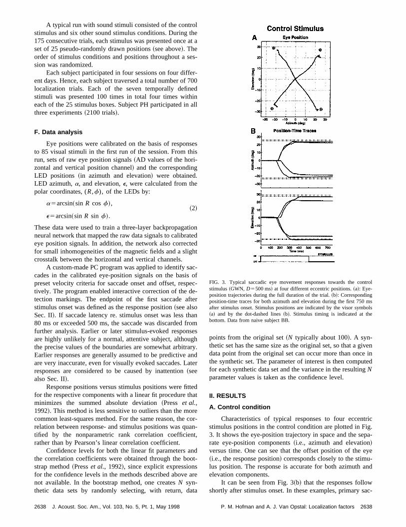
Characteristics of typical responses to four eccenstimulus positions in the control condition are plotted in F3. It shows the eye-position trajectory in space and the serate eye-position components~i.e., azimuth and elevation!versus time. One can see that the offset position of the~i.e., the response position! corresponds closely to the stimulus position. The response is accurate for both azimuthelevation components.

It can be seen from Fig. 3~b! that the responses followshortly after stimulus onset. In these examples, primary s

FIG. 3. Typical saccadic eye movement responses towards the costimulus~GWN, D5500 ms! at four different eccentric positions.~a!: Eye-position trajectories during the full duration of the trial.~b!: Correspondingposition-time traces for both azimuth and elevation during the first 750after stimulus onset. Stimulus positions are indicated by the visor sym~a! and by the dot-dashed lines~b!. Stimulus timing is indicated at thebottom. Data from naive subject BB.


s

re

e

utyelor

-ssoo

ctas

over

g.in

azi-uth

r-the

utheva-tirefor

io-

u

ithse-

. Forthe

t offor

x is

vation

cades are initiated with a latency of approximately 200 mand are completed within 400 ms after stimulus onset~i.e.,before stimulus offset time!.

All subjects in this study made accurate localizationsponses to the control stimulus~500-ms GWN! in all direc-tions ~azimuth and elevation!. Figure 4 shows all saccadtrajectories@Fig. 4~a!# and saccade endpoints@Fig. 4~b!# forall four sessions of one of the subjects~BB!. Note how boththe stimulus positions and saccade trajectories are distribover the entire stimulus range. Note also, that the accuracresponse elevation is both quantitatively and qualitativsimilar to azimuth localization. A summary of the results fall subjects is listed in Table I.

Figure 5~b! gives an overall impression of the local localization accuracy by showing the averaged signed errorthe saccadic responses for each stimulus box. For eachject and each stimulus box, the mean signed error was cputed for all responses to stimuli presented within that b

FIG. 4. Saccadic responses to the control stimulus.~a! Trajectories of pri-mary saccades~thick dotted lines, sampled at 2-ms intervals! to controlstimuli presented throughout the entire stimulus range. Stimulus positare indicated by the visor symbols.~b! Endpoint positions of the same primary saccades as in~a! versus stimulus positions for both azimuth~s! andelevation~d!. Also the linear-fit results for response positions versus stimlus position are provided~azimuth:aS vs aR ; elevation:eS vs eR!. Notelarge slopes~0.97 and 0.90, respectively;N598! and small offsets~within 2deg!. Subject BB.


,

-

edofy

ofub-m-x

~typically 4–8 responses for each box and each subje!.Then, a final mean signed error for each stimulus box wobtained by averaging the subject-mean signed errorsall 7 subjects.

Note that, for the majority of the error boxes in Fi5~b!, the height is larger than the width. Thus the scatterthe responses is somewhat larger for elevation than formuth. These scatter properties underline the fact that azimand elevation localization are dissociated processes~see theIntroduction!. They clearly contrast with the scatter propeties of visually evoked saccadic responses, that betraypolar organization of the visuomotor system~e.g., Van Op-stal and Van Gisbergen, 1989!.

One may observe that the highest accuracy for azimlocalization is reached near the median plane, whereas eltion accuracy is approximately homogeneous over the enoculomotor field. The largest signed errors were found

ns

-

FIG. 5. ~a! Stimulus positions were presented within the square boxes, wdimensions 838 deg. Sets of 25 stimulus positions were composed bylecting a position at random within each box.~b! The lines from the opensymbols to the closed symbols correspond to local mean signed errorseach stimulus box, the mean signed error is computed by averagingindividual mean signed errors of all seven subjects. The width and heigha box correspond to twice the standard deviation in the signed errorsazimuth and elevation, respectively. The center of each stimulus boindicated by the open circle@in both ~a! and ~b!#. Note the clear separationof almost all response boxes, and the larger response scatter in the elecomponents as compared to the azimuth components.

usn

–7:fit

ectively,

TABLE I. Parameters of the azimuth~a! and elevation~e! response components to the control stimul~500-ms white noise! for each subject. Columns 2–3: rank correlation coefficientr between response positioand stimulus position. Note that correlation coefficientsre.0.90 for elevation andra.0.95 for azimuth.Columns 4–5: slope, or gain,G, of a straight-line fit for response versus stimulus position. Columns 6standard deviationDFIT of the difference between the actual response and the response predicted by the~indegrees!. Columns 8–9: average absolute localization errorDRESP ~in degrees!. Column 10: median responslatency~in ms!. The two bottom rows present, for each column, the mean and standard deviation, respepooled for all subjects.

Subject

Corr r Gain G DFIT DRESP

Lat.a e a e a e a e

JO 0.97 0.91 1.1 0.67 4.3 4.9 5.1 6.3 166BB 0.97 0.94 0.97 0.90 4.5 6.2 3.3 4.9 198VC 0.96 0.91 0.96 0.81 5.0 6.8 3.8 8.3 226KH 0.96 0.92 1.0 0.88 5.7 5.5 5.2 4.6 244JR 0.97 0.95 1.1 1.1 5.0 6.9 4.3 5.9 148JG 0.97 0.93 1.3 1.0 4.6 6.4 5.4 7.8 156PH 0.98 0.95 1.1 1.1 3.9 5.9 4.4 6.4 166

mean 0.97 0.93 1.06 0.91 4.6 6.0 4.5 6.3 186s.d. 0.01 0.02 0.11 0.15 0.7 0.8 0.9 1.5 38


t

i

ur

e

-,ic

r

ev

iszens.lias

lusde

ege,

ially

for

tio

pro

-

u-or

stimulus positions within the box at (a,e)5(0,213) deg,where response elevations were, on average, abou65 deg lower than the actual stimulus elevations.

B. Test conditions

Typical responses to four eccentric stimulus positionsone of the test conditions~noise burst, durationD53 ms! areplotted in Fig. 6. It is clear that azimuth localization is accrate. However, in contrast to the control condition, wheelevation detection was also accurate, the responses nowhibit large undershoots in elevation.

Typical responses for the three different stimulus typemployed in this study are shown in Fig. 7~data from sub-jects BB, JR, and PH, respectively!. The most obvious feature of these data, obtained for all three test conditionsthat the saccade trajectories cover only part of the vertstimulus range@compare Fig. 7~a! with Fig. 4~a!#. Comparedto the control condition~see Fig. 4!, localization accuracyhas clearly deteriorated for elevation, whereas it hasmained the same for azimuth@Fig. 7~b!, open symbols#.However, although elevation accuracy has deterioratedthese test conditions, the correlation between stimulus el

FIG. 6. Typical responses toward short-duration noise bursts (D53 ms) atfour different eccentric positions. Note marked undershoot of the elevacomponents, whereas the azimuth components remain accurate~cf. Fig. 3!.Note further that also small secondary saccades are made after apmately 400 ms. See legend of Fig. 3 for further details.


8

n

-eex-

s

isal

e-

ina-

tion and response elevation is still highly significant. Thcan also be seen in Tables II, III, and IV, which summarithe regression results for all subjects and the test conditio

In summary, we found for all spectro-temporal stimuthat, although response elevation could be incorrect, it wquite consistent and correlated highly with the real stimuelevation:re>0.4 for all conditions. This is also expresseby the difference,DFIT , between the responses and thstraight line fits~dashed lines in Fig. 4 and Fig. 7!: DFIT

remained within 4–8 deg for elevation and within 3–6 dfor azimuth for all stimulus conditions and subjects. Hencthe variance in the responses did not increase substantwith respect to the control condition~compare with Table I!.

C. Response gain

Next, we compared the responses for each subjectthe different temporal parametersD, DT, and T with theresults from the control stimulus (D5500 ms). The straight

n

xi-

FIG. 7. Saccadic responses to test stimuli.~a! and ~b! responses of subjectBB to noise bursts of durationD53 ms~correlations for azimuth and elevation: ra50.97, re50.69; N595!. ~c! and ~d! responses of subject JR topulse trains with duty cycleDT540 ms ~ra50.97, re50.86; N597!. ~e!and ~f! responses of subject PH to FM sweeps with periodT520 ms ~ra

50.96,re50.38; N5143!. Correlations for response position versus stimlus position are listed in Tables II, III, and IV. See legend of Fig. 4 ffurther details.


s

2641 J. Acoust. S

TABLE II. Parameters of the responses to noise-burst stimuli with various durationsD ~in ms! for threesubjects. Note that elevation gain increases systematically with increasingD, but that the variability in the data(DFIT) is independent ofD. Azimuth gain, however, is not affected byD. Note also, that the median latencietend to decrease asD increases. See Table I for further explanation of the columns.

Subject D


Lat.a e a e a e a e

BB 3 0.97 0.69 0.85 0.22 4.9 5.9 4.9 13 2105 0.96 0.71 0.81 0.33 5.5 6.4 5.1 11 213

10 0.96 0.79 0.86 0.30 5.1 4.8 4.7 11 20720 0.97 0.89 0.87 0.50 5.4 5.6 4.4 9.1 19140 0.97 0.94 0.91 0.63 4.6 5.3 3.7 6.7 18880 0.95 0.94 0.90 0.76 6.4 5.8 5.0 5.7 190

JO 3 0.98 0.80 0.99 0.28 3.4 4.1 4.7 12 1825 0.98 0.76 1.0 0.35 3.4 5.1 4.1 11 180

10 0.97 0.80 1.0 0.43 3.8 5.0 4.4 10 17320 0.97 0.88 1.0 0.42 4.1 4.6 4.3 9.8 16440 0.96 0.92 1.0 0.56 4.3 4.4 4.8 7.2 16480 0.97 0.92 1.1 0.61 4.0 4.8 4.7 7.0 163

PH 3 0.97 0.85 1.1 0.67 4.4 8.0 4.4 10 1885 0.97 0.87 1.1 0.70 4.2 7.1 4.4 9.4 180

10 0.97 0.87 1.1 0.82 4.6 7.5 4.7 10 17220 0.96 0.89 1.1 0.81 4.4 7.1 4.9 8.3 16440 0.98 0.93 1.1 0.99 3.3 6.2 3.7 6.7 16480 0.97 0.94 1.1 1.0 4.1 6.0 4.2 6.1 162

tioethsey

ct

it

tion

ctub-vetrolrstise

line appeared to yield a reasonable description of the relabetween response versus stimulus position, and the slopthe line turned out to be a characteristic parameter forresponses in a given condition. One can immediatelyfrom Fig. 8 that the response gains for elevation varied stematically with all three temporal parameters~bottom pan-els!. The azimuth component of the saccades was unaffeby the stimulus parameters~top panels!.

For the noise burst, the same systematic variation w

oc. Am., Vol. 103, No. 5, Pt. 1, May 1998

nofee

s-

ed

h

D is observed for all three subjects: the response elevagain increases gradually with stimulus durationD, from D53 ms up toD580 ms. Although there is some intersubjevariability as to the absolute values of these gains, all sjects followed a similar trend. Note that similar quantitatiinter-subject differences were also obtained for the constimuli. Furthermore, as the control stimulus is a noise buwith D5500 ms, the results suggest that for broadband nobursts responses stabilize at roughlyD580 ms. Note that the

the

TABLE III. Parameters of the responses to the burst-train stimuli with various duty cyclesDT ~in ms!.Elevation gain, but not azimuth gain, depends systematically onDT. DT5` refers to the single 3-ms bursstimulus. Median latencies tend to decrease withDT for all three subjects. See Table I for explanation of tcolumns.

Subject DT


Lat.a e a e a e a e

JR 3 0.98 0.94 1.1 1.1 4.4 6.9 3.8 6.4 14810 0.98 0.93 1.1 1.0 4.4 7.3 3.9 5.7 15420 0.98 0.90 1.2 0.86 4.2 7.7 4.0 7.0 16040 0.97 0.86 1.1 0.69 5.0 7.7 4.2 8.6 16680 0.97 0.85 1.1 0.61 4.9 6.7 4.0 8.9 168` 0.96 0.74 1.1 0.49 5.1 7.8 4.2 10 166

JG 3 0.98 0.94 1.2 1.0 4.4 5.9 5.2 6.6 15610 0.98 0.87 1.2 0.82 4.1 7.7 4.9 8.0 15820 0.96 0.93 1.2 0.73 5.5 4.7 5.6 7.1 16640 0.97 0.92 1.2 0.77 4.8 5.8 5.5 7.1 17080 0.97 0.92 1.3 0.77 4.9 6.2 5.7 6.1 182` 0.97 0.83 1.3 0.55 5.7 7.9 6.8 12 176

PH 3 0.98 0.92 1.1 1.0 4.4 7.5 4.2 6.1 16410 0.97 0.96 1.1 0.97 4.4 5.1 4.1 5.8 17820 0.97 0.91 1.1 0.83 4.3 6.5 4.6 9.0 17040 0.97 0.91 1.1 0.71 4.3 6.0 4.7 10 18280 0.97 0.82 1.1 0.59 4.0 6.9 4.7 11 190` 0.97 0.84 1.1 0.76 4.4 8.1 4.5 11 182


2642 J. Acoust. S

TABLE IV. Parameters of the responses to sweep stimuli with various repetition periodsT ~in ms!. Elevationgain, but not azimuth gain, depends systematically onT. Median latencies tend to increase withT for subjectPH, but not for subjects VC and KH. See Table I for explanation of the columns.

Subject T


Lat.a e a e a e a e

VC 1.3 0.95 0.79 0.92 0.58 5.4 8.5 4.4 13 2442.6 0.96 0.87 0.84 0.63 4.2 7.2 4.5 9.8 2325.1 0.96 0.70 0.86 0.27 5.0 6.9 5.2 12 236

10 0.95 0.55 0.87 0.15 5.4 6.8 4.8 13 23720 0.96 0.43 0.94 0.14 5.4 5.8 4.6 14 23441 0.95 0.47 0.97 0.15 5.6 7.2 4.7 14 240

PH 1.3 0.97 0.91 1.1 0.91 4.3 7.2 4.0 10 1642.6 0.97 0.91 1.1 0.81 5.6 7.6 4.7 6.5 1635.1 0.96 0.86 1.0 0.64 4.8 6.9 4.0 7.9 170

10 0.97 0.43 1.2 0.15 5.3 8.1 5.5 14 16820 0.96 0.38 1.1 0.12 4.8 6.5 4.3 14 18841 0.96 0.63 1.2 0.20 6.2 4.1 7.1 14 184

HK 1.3 0.94 0.84 0.95 0.55 5.7 7.1 4.9 8.3 2512.6 0.95 0.84 0.81 0.66 5.3 7.4 5.0 8.4 2465.1 0.96 0.85 0.94 0.43 4.7 5.0 4.4 12 269

10 0.95 0.57 0.87 0.29 4.8 7.5 4.3 15 24320 0.93 0.41 0.79 0.13 4.7 5.9 5.3 20 25841 0.97 0.60 0.93 0.19 4.6 5.3 3.9 18 239

fo%

s

gn-i-ororr

fogle

lit

te

ttho

e,

.

ber

the-ive

that

of

C,ghwereed

wnnts.

e du-ob-

,

d asM

-e-

as avalwas-

short bursts already account for relatively large gains:example, the gains atD510 ms are already about 40%–80of the final gains obtained forD580 ms.

For the burst-train stimulus, response gain decreamonotonously with the duty cycleDT for subjects PH andJR. The response gain of subject JG, although displayinsimilar overall trend, does not vary significantly for the itermediate values ofDT510,20,40,80 ms. In this experment, the intersubject variability for the gains is small fboth the burst trains and the control condition. For the shest duty cycles applied (DT53 ms), the gain is similar as fothe control condition~indicated by C!. In addition, for sub-ject PH who also participated in experiment I, the gainDT580 ms is very similar to the gain observed for the sinnoise burst atD53 ms~conditionD3 in Fig. 8!. This resultcould be expected: the latency of this subject’s responsearound 150 ms~see Table III!, so that only the first burs~i.e., at t50 ms! and maybe the second one~at t580 ms!could actually have been processed by the auditory sysfor generating the first saccade.

For the sweeps, the elevation gain decreases whenperiod T increases. In contrast to the noise burst andburst train, the change with the temporal parameter is msudden. ApproximatelyT55 ms seems to be a critical valuwhere the response elevation changes most rapidly withT.From T510 ms~subject KH! or T520 ms~subjects PH andVC! there is little change in the gain which lies between 0and 0.2. Although the gains forT>10 ms are relatively low,correlations for the sweep data were still 0.38 or higher.

D. Response latency

The latencies of primary saccades are typically welllow 300 ms. Figure 9~a! shows a latency distribution fosaccades to the control stimulus~subject PH!. One can see

oc. Am., Vol. 103, No. 5, Pt. 1, May 1998

r

es

a

t-

r

es

m

heere

1

-

that latencies peak near 170 ms and remain within@100,300#-ms interval. This interval was typical for all subjects, which can be further appreciated from the cumulatlatency distributions in Fig. 9~b!. Data from three differentsubjects for the control condition are presented: latencieswere relatively short~subject JR!, long ~VC!, and intermedi-ate ~PH!. Note that, also for subject VC, more than 90%the latencies remained below 300 ms.

It may be observed that in Fig. 9~b! the curves are nearlylinear and roughly parallel to each other~see Sec. III!. This ismost obvious for the distributions of subjects PH and Vwhich are well-defined, since they consist of a relatively hinumber of saccades. For other subjects, fewer saccadesavailable for each condition, but the distributions exhibitroughly similar [email protected]., subject JR, Fig. 9~b!#.

For subject PH, also cumulative distributions are shothat resulted from the several short-noise burst experimeOne can see that latencies systematically increase as thration of the noise burst decreases. The same trend wasserved for the other subjects~BB, JO! who participated inthis experiment~see Table II!. Also in the other experimentsa systematic shift of the~reciprocal! latency distribution asfunction of the temporal stimulus parameter was observewell ~except for subjects VC and KH in response to Fsweeps!. Median latencies also show this trend~see TablesII, III, and IV !. For different stimulus conditions, the reciprocal latency distributions differed in their offset, but rtained their shape.

E. Primary and secondary saccades

The endpoint of the primary saccade was acceptedvalid response when its onset latency fell in the inter@80,500# ms. For the average subject, a valid responsemeasured in 97%62% of the trials. In the same time inter


tic

anbj

ng

ars

art,ed

rgadn,os-cth

ntsheysoralif-

ith

tro-ed

o-heous-lts

s un-the

per-odthehe

ntscedrmsed

thee

nn

f t

sn

tiv

ects aat, aheH;thinrsts

val, a secondary saccade was observed in 23%69% of thetrials, and a third saccade in less than 4% of the trials.

To test whether the secondary saccade was correc~which is known to be the case for visually evoked sacades!, the unsigned errors after the primary saccade,after the secondary saccade were compared for each suThis was done for saccade azimutha, elevatione, amplitudeR and directionf. The analyses revealed that incorporatithe second saccade did not significantly change~i.e. neitherimprove nor deteriorate! response accuracy~data not shown!.

To further check for a possible relation of the secondsaccade with the stimulus position, an additional analywas performed by comparing the directions of the primsaccade, the secondary saccade and the stimulus. Firsdifference in direction,Df12 between the primary and thsecondary saccade was computed. For all subjects poolewas found thatDf1254648 deg. The individual results foeach subject were similar. Thus the secondary saccadeerally proceeds in the same direction as the primary saccNext, Df12 was compared to the difference in directioDf01, between the primary saccade and the stimulus ption ~i.e., the direction error!. No significant correlation betweenDf12 and Df01 was found. Thus the secondary sacade does not correct for a residual direction error afterprimary saccade either.

FIG. 8. Response gains for all subjects and all conditions. The gaidefined as the slope of the straight line fitted through response compoversus stimulus component~see also Fig. 4 and Fig. 7!. Top panels: azimuthgains. Lower panels: elevation gains. Gains are plotted as function otemporal stimulus parametersD, DT, andT. The control condition is indi-cated by C. The single-burst condition in the burst-train experimentlabeled by D3. Optimal agreement of response and stimulus positioassociated with gain 1.0~dashed lines!. Lowest correlationsre obtained fornoise bursts, burst trains and sweeps were 0.58, 0.83, and 0.38, respecbut still highly significant~see Tables II, III, and IV!.


ve-d

ect.

yisythe

, it

en-e.

i-

-e

III. DISCUSSION

A. General findings

In the present study, human localization experimewere performed using a wide range of acoustic stimuli. Ttime-averaged power spectra of the stimuli were alwabroadband and identical in shape, but the spectro-tempbehavior on a millisecond time scale was fundamentally dferent. Localization performance varied systematically wthe experimental parametersT, DT, andD. Whereas eleva-tion detection appeared to be very sensitive to the spectemporal stimulus behavior, azimuth localization remainunaffected and was equally accurate for all conditions.

Our findings provide new insights into the spectrtemporal processing of acoustic sensory information. Tdata suggest specific temporal constraints for accurate actic localization of stimulus elevation. Moreover, these resuunderline the presence of separate dynamical processederlying the analysis of the different acoustic cues fordetection of azimuth~ITD, IID ! and elevation~spectral shapecues!.

B. Saccadic eye movements

1. Orienting to sounds through saccadic eyemovements

Saccadic eye movements were used to measure theceived sound direction. The results show that this methyields a highly reproducible and accurate measure ofacoustic localization percept for stimuli presented within toculomotor range~approximately 35 deg in all directions!.Correlations for both the horizontal and vertical componeof responses to control stimuli exceeded 0.9 in experienas well as in naive subjects. The oculomotor response foan important part of the natural repertoire of stimulus-evokorienting~including head and body movements! and does notrequire any specific training of the subjects. Moreover,response is fast~latencies remain well below 300 ms; sealso Frens and Van Opstal, 1995!.

isent

he

isis

ely,

FIG. 9. ~a! Response latency distribution for the control condition. SubjPH. ~b! Cumulative response latency distributions. The latency axis hareciprocal scale, whereas the abscissa is on probit scale. In this formGaussian distribution of reciprocal latency results in a straight line. Tthick dotted lines refer to the control conditions for subject JR, VC, and Pthe distributions consist of 99, 219, and 398 saccades, respectively. Thelines show the cumulative distributions of responses to short noise buwith D53, 5, 10, 40 ms~subject PH!. For each conditionD, about 116saccades are included.


tsn

-asinaeagb

arstoaca

ecuonetherla

ysilrut

elthist

otees

thcu

ncanad

re

ori-.lop-nal, ini-

-he

Ifre-

atatia-

in

ns.am-velesh-areinceec-hew-ore

hers

ngby

s.thec-ro-s

s of

on-t theation,

In previous localization studies with human subjecdifferent response methods have also been used to quathe localization percept: arm pointing~e.g., Oldfield andParker, 1984a!, the naming of learned coordinates~e.g.,Wightman and Kistler, 1989!, and head pointing~e.g., Mak-ous and Middlebrooks, 1990!. The first two methods are substantially slower than the eye-movement method and mthus be assumed to measure a later acoustic percept, posalso incorporating cognitive aspects. The head-pointmethod is potentially faster. Although latencies of hemovements can be similar to eye movement latencies, hmovements dynamically alter the acoustic input for londuration stimuli, which was deemed to be an undesirafactor for the purpose of this study.

2. Potential artefacts

We are confident that our main results cannot becribed to peculiar properties of the oculomotor system. Fithe sound stimuli were presented well within the oculomorange and stimulus types and stimulus positions were alwpresented in a randomized order. Therefore, the resultsnot be due to a~conscious or subconscious! strategy adoptedby the subjects.

A second argument for believing that the results reflproperties of the auditory system, rather than of the vismotor system, is that quite different behaviors were obtaifor the azimuth components of the responses, than forelevation components. Such a behavior is never encountin visually evoked eye movements toward stimuli at similocations.

We also believe that the auditory stimuli were alwapresented well above the detection threshold, since simtemporal-dependent response behaviors were obtained fothree acoustic stimulus types. The finding that the azimcomponents of the responses remained unaffected bystimulus parameters, indicates that the stimuli were wperceived by the auditory system, despite the fact thatoverall acoustic energy of the stimuli varied greatly. Thisalso supported by the fact that the standard deviations oflatency distributions were hardly affected@see Fig. 9~b!, andbelow#.

Finally, also the result that response variability did nchange systematically with the temporal stimulus parame~Tables II, IV, and III! argues against the possibility that thauditory stimuli may have been close to the detection threold for the shortest stimulus durationsD or longest dutycyclesDT.

3. Latency characteristics

There are some interesting aspects regardingauditory-evoked saccadic latency distributions. First, themulative latency probabilities in Fig. 9~b! are plotted on aso-called probit scale, which is the inverse of the Error fution. If the cumulative distribution on probit scale yieldsstraight line, the variable follows a Gaussian distributioThis linear feature of reciprocal latency distributions hbeen shown to be characteristic for visually evoked sacca~Carpenter, 1995!. In the present study, straight lines we


,tify

yiblygdd--le

s-t,rysn-

t-deedr

arall

thhel-e

he

trs

h-

e-

-

.ses

also obtained for auditory saccades, despite the differentgin and encoding format of acoustic sensory information

Carpenter~1995! proposed a simple model for visuasaccade initiation that accounts for this characteristic prerty ~Fig. 10!. The model assumes that a decision sigstarts to increase after stimulus onset and, subsequentlytiates the saccade upon exceeding a fixed threshold (u0).Consequently, the time-to-threshold~i.e., the saccade latency! is inversely proportional to the increase rate of tdecision signal. The increase rate~slope a! is assumed tovary from trial to trial, but remains constant during a trial.this rate is distributed as a gaussian over trials, then theciprocal latency is necessarily distributed likewise. Our dsuggest that a similar mechanism could underlie the inition of auditory-evoked saccades.

Yet, the question remains how stimulus-related shiftsthe distributions could arise. For example, Fig. 9~b! showsthat latencies become larger for shorter stimulus duratioThe simple model described above has only a few pareters that can cause a shift in the distribution: the initial leof the decision signal, its mean increase rate, and the throld level. The first two parameters have preset values andassumed to depend on expectation about the stimulus. Sthe different stimuli were presented in random order, exptation is not likely to play a role in the present situation. Tshift in the median latencies is qualitatively explained, hoever, if it is assumed that the threshold decreases as msensory information comes in (uD). For short burst dura-tions, the threshold would then remain systematically hig~yielding longer latencies! than for longer stimulus duration~see also Fig. 10!.

4. Secondary saccades

The typical response pattern of an auditory orientitrial usually consists of a large primary saccade followeda smaller secondary~and occasionally a tertiary! saccade. Asimilar pattern is also typical for visually elicited responseThe primary saccade carries the eye over roughly 90% ofrequired trajectory~undershoot!, whereas the secondary sacade corrects for the remaining retinal error. It has been pposed~Harris, 1995! that such a motor strategy minimize

FIG. 10. A simple model that accounts for the observed characteristicthe latency distribution~see also Carpenter, 1995!. At stimulus onset, adecision signal rises with a constant rate,a, and upon exceeding a fixedthreshold, atuD , a saccade is initiated. In each trial, the increase rate,a, isdrawn from a gaussian distribution. In order to incorporate the conditidependent modulations on the latency in this study, it is proposed thathreshold is not constant, but instead decreases during stimulus presentfrom the initial valueu0 to the final valueuD .


yioti

te

estroftengta

ctthTm

angiorrdndertl

inan

ala

rethc

g

f

pafeesfohes

tr

celt

mero-n-

kepts

-Al-

s ofon-as

emolu-

ry

-in-rm

at aa

nts

rmcle

i-m

theget

init

ests in

al-

e-inwn

ve-

helyro-e of

pri-with

~in a statistical sense! the time needed to fixate the target, btaking into account both the effects of a longer duratneeded to complete larger saccades, and the additionalneeded to program a corrective saccade in the oppositerection ~due to an overshoot!. Here, the question was whathe underlying strategy for secondary saccades could bthe case of a sound stimulus.

Analysis of the auditory responses indicated that the sondary saccades were not corrective. Note that, in contravisual stimulus conditions, the oculomotor system is not pvided with any feedback concerning its performance acompleting the primary auditory saccade. Notwithstandithe occurrence of a small secondary saccade in roughlysame direction as the primary saccade was quite typical insubjects tested. We propose that this phenomenon refleproperty of the programming mechanisms underlyingoculomotor response, rather than auditory processing.data suggest that the secondary saccade is a pre-programmovement that in this case, however, does not~cannot! cor-rect for a residual error.

C. Temporal aspects of sound localization

1. Effect of stimulus duration

It should be realized, that the programming ofauditory-evoked saccade consists of at least two main staa target localization stage, in which the acoustic informatis transformed into an estimate of target location, and asponse initiation stage in which the estimated target coonates are transformed into the appropriate motor commaWe believe that the data obtained from the noise-burstperiments may be interpreted in the light of these two, paseparate, stages.

First, it was found that the response elevation gaincreases systematically as function of stimulus duration,that it reaches a plateau for stimulus durations exceedingms ~Fig. 8!. From these data we infer that the auditory locization system needs roughly 80 ms of Gaussian broadbinput to reach a stable estimate of target elevation.

Second, the latency data@Fig. 9~b! and Table II# mayprovide further insights into the processing time of thesponse initiation stage. Although it takes less time forshort-duration bursts to complete, the associated latenwere about 20 ms longer than for the longest stimuli~seeTable II!. This suggests that the movement initiation statakes, at least, about 20 ms longer to initiate a saccadeward the shortest burst. We have no simple explanationthis apparent, yet consistent, discrepancy.

In contrast to sound elevation, sound azimuth can apently be determined accurately on the basis of only amilliseconds of sensory information. Even for the shortstimuli (D53 ms), the accuracy was about the same asthe control condition (D5500 ms). In this sense, azimutlocalization can be considered as a much ‘‘faster’’ procthan elevation localization. From our data it is not possibleconclude whether this property is due to mechanisms pcessing either the interaural phase or intensity differensince the broadband bursts provided both cues simuneously.


nmedi-

in

c-to-r,

hell

s aehe

ed

es:ne-i-s.

x-y

-d

80-nd

-eies

eto-or

r-wtr

soo-s,a-

2. Effect of nonstationarity of the short-termspectrum

The results obtained from the FM sweeps provide sofurther interesting suggestions regarding the temporal pcessing of sensory information in sound localization. In cotrast to the noise bursts, the duration of the sweeps wasconstant~at 500 ms!, but the spectro-temporal behavior wavaried by means of the cycle variableT. Response characteristics were similar as in the case of the noise bursts.though elevation localization accuracy varied withT, re-sponses remained consistent: high correlation coefficientresponse versus stimulus position were obtained for all cditions. Because elevation localization performance wmost accurate forT,5 ms and relatively inaccurate forT.5 ms, it is suggested that the auditory localization systdiscriminates spectro-temporal patterns at a temporal restion down to about 5 ms.

A possible explanation for this ability is that the auditosystem applies a so-calledmultiple-lookstrategy~e.g., Vie-meister and Wakefield, 1991!. In such a mechanism, the input spectrum is measured over consecutive short time wdows, each lasting only a few milliseconds. Each short-tespectrum is processed into a position estimate, which,higher level, is integrated with the earlier estimates intofinal estimate~see below, Fig. 12!. This explanation is also inline with the interpretation of the burst-duration experime~see above!.

As an example, consider the computation of a short-tespectrum over a 5-ms time window somewhere in the cyof an FM sweep with a long period, e.g.,T520 ms. Theoutcome will vary substantially for different window postions within the cycle. Elevation updates computed froconsecutive~but very different! short-term spectra wouldthen be inconsistent throughout the cycle and preventdynamic elevation estimate to stabilize at the actual tarelevation. Note, that such a 5-ms time-averaged spectruma fast sweep (T,5 ms) would be broadband, whereaswould be narrow band for very slow sweeps (T@5 ms).

3. Effect of silence gaps in the stimulus

The data obtained from the burst-train stimuli suggfurther constraints on the dynamics of the spectral analysithe localization process. For the shortest burst intervals,DT,near-optimal localization performance was obtained,though each burst was only 3 ms long.

Interestingly, the elevation gain was observed to dcrease significantly when the individual bursts of the trawere all chosen to be identical, rather than randomly draas in the experiments presented here, even forDT53 ms~data from subject PH only, not shown!. Thus acoustic inputpresented at later times indeed contributes to the improment of the final elevation estimate.

The low gains at long intervals are not explained by tfact that, within the latency period of roughly 180 ms, ontwo to four 3-ms bursts may have contributed to the pgramming of the first saccade, because the final estimatthe oculomotor responses~even after 500 ms! was not sys-tematically better than the estimate recorded after themary saccade. Rather, the decrease of elevation gain


stt

ha

fo

rade,or

o

ae

eshereme

e

,

ce

ro

m

vel-

se-

ith

mp-anachghlytaine-nal

ag-

oursandther-

increasingDT indicates that the subsequent elevation emates, based on each 3-ms sound burst, are not kepacoustic memory forever. Possibly, the integrative mecnism that combines subsequent elevation estimates~seeabove! is leaky. If so, the data suggest a time constantthis integrator in the order of a few tens of ms.

D. Toward a spectro-temporal model of soundlocalization

In this section we study the properties of a monaulocalization model that relies on spectral correlations in orto estimate sound elevation,eS ~see also Middlebrooks1992!. In addition, a biologically plausible mechanism fthe dynamic implementation of these correlations, basedour data, will be briefly described.

1. Spectral correlations

In the proposed spectral correlation approach, it issumed that the auditory system bases its comparison betwthe sensory signal and the HRTF on the log power of thspectral functions. In addition, a logarithmic scaling of tfrequency domain, reminiscent to the tonotopic neural repsentation of sound frequency throughout the auditory systis applied. By applying the logarithm to the power of thsensory signal measured at the eardrum, Eq.~1! can be re-written as:

Y~v;eS!5H~v;eS!1X~v!, ~3!

wherev is in octaves, andeS is the source elevation. Thcapitals indicate the logarithmic power [email protected]., X(v)[ logux(v)u#. Note, that elevation,eS , rather than positionrS , is used in Eq.~3!, as it is assumed that azimuth,aS , isalready extracted from binaural cues.

A quantitative scalar measure of similarity for two spetral functions can be given by the spectral correlation coficient. Therefore, the mean,F, and variance,sF

2, for anarbitrary spectral function,F(v), are first introduced:

F5^F~v!&[E0

`

dv p~v!F~v!,

~4!

sF25^~F~v!2F !2&,

with p(v) a normalized weighting function that is nonzein the ~broad! frequency band of interest. Herep(v) waschosen to be uniform in the@2, 16# kHz range, and zeroelsewhere. The spectral correlation,C„F(v),G(v)…, be-tween two functions,F(v), and,G(v), is then defined as

C„F~v!,G~v!…[K S F~v!2F

sFD S G~v!2G

sGD L . ~5!

The outcome varies in@21,1#, whereC(•)51 correspondsto ‘‘maximal similarity,’’ and C(•)<0 means ‘‘no similar-ity.’’

In the present discussion, the spectral correlation copares the sensory signal,Y(v;eS), with ~neurally stored!HRTFs,H(v;e), for all sound elevationse. By using Eq.~3!and by taking the mean~whereY5HS1X!, this comparisonreads:


i-in-

r

lr

n

s-ene

e-,

-f-

-

CY~e;eS![C„Y~v;eS!,H~v;e!…

5S sHS

sYDC„H~v;eS!,H~v;e!…

1S sX

sYDC„X~v!,H~v;e!…

[S sHS

sYDCH~e;eS!1S sX

sYDCX~e!, ~6!

with sY , sHS, sX the standard deviations of the respecti

quantities in Eq.~3!. Thus Eq.~6! quantifies the spectracorrelation of each stored HRTF~associated with sound elevation,e! with the measured spectrum at the eardrum~re-sulting from a sound source at elevation,eS!. It proposed thatthe perception of sound elevation essentially consists oflecting the unique positione5eP at which the global maxi-mum, CY(eP ;eS), is attained.

In its decomposed form, Eq.~6! can be readily inter-preted. The first term on the right-hand side,CH(e;eS), isthe spectral correlation between the HRTFsH(v;e) andH(v;eS). Under the assumption that HRTFs are unique wrespect to position,CH(e;eS) reaches a maximum in theneighborhood ofeS , i.e., ate'eS .

Figure 11 shows that this is indeed a reasonable assution. In this figure, measured HRTF functions in the mediplane of one of our subjects have been correlated with eother. Note that only along the principal diagonal a hicorrelation is obtained, indicating that, indeed, HRTFs onresemble themselves. Therefore, these functions conunique information about target elevation, when all frquency bands are allowed to contribute to the computatio

FIG. 11. Spectral correlations of human HRTFs, measured in the midsgital plane at elevations$235,230,...,150,155% deg. Subject PH. Thestrength of the correlation is coded by brightness. Markers label the contat different values. Note that HRTFs correlate strongest with themselveswith HRTFs at neighboring elevations. Correlations were computed infrequency range@2,16# kHz and HRTFs were sampled at 1/20 octave intevals.


ound,

Feonation,

FIG. 12. Conceptual spectro-temporal correlation model of human sound localization. The first stage represents the auditory periphery, where a sx(t),at elevation,eS , is processed from the external ear up to the cochlea. In the second stage, a short-term~order a few ms! averaged spectrum,Y(v,t;eS), isdetermined around the current time,t, from the ongoing sensory spectrum,Y(v,t;eS). Then, Y(v,t;eS) is correlated with the neurally stored HRTrepresentations,H(v;e), for all possible elevationse, i.e.,e1 ,...,eN , yielding short-term correlationsC(e,t;eS). Next, integration is done over a longer timspan~order several tens of ms!, resulting in a long-term correlation up to current timet, C(e,t;eS). This integration process may be leaky. In the decisistage, the average correlation at timet yields a perceived elevation,eP(t). It is proposed that this decision depends on the maximum of the average correlbut also on the consistency of that average and on the initial elevation percept.

f

n

in

-

te

n

ch.e

th

li-

tic

coo

thiotooncootra

iva

tione of

t-

tion

ent

on

tingion

g ishe

a-

ab-iza-va-g

sys-azetialrth-d-ef-lus

Joseleforlsom-

process. We have verified that this conclusion also holdsthe entire elevation domain~eP@260,90# deg, front andback!, although the region of maximum correlation broadeappreciably close to zenith positions~e'190 deg; data notshown!. It is therefore expected, that stimuli presented withthat range are not well localized and discriminated.

The second term in Eq.~6!, CX(e), expresses the resemblance of the source spectrumX(v) with each particularHRTF H(v;e). If the source spectrum does not correlasignificantly with any of the stored HRTFs, thenCX(e)'0for all e @for example, this would be true ifX(v) is flat andbroadband#. In that case, the maximum correlatioCY(eP ;eS) will be reached ateP5eS , thus the sound wouldbe accurately localized. It is expected that there will bebroad range of naturally occurring acoustic stimuli for whithere is little or no resemblance with the stored HRTFs, iCX(e)'0.

However, the second term does come into play, ifsource spectrumX(v) does correlate well with a givenHRTF, sayH(v;e* ). This occurs ifX(v) contains promi-nent features that are characteristic forH(v;e* ). Then,CX(e* )@0, meaning thatCY(e;eS) contains a second locamaximum ate5e* . This could even be the global maxmum in which case the perceived position,eP , would be,e* , rather than the actual position,eS , thus eP5e* ÞeS .This might occur, for example, whenX(v) is narrow band~i.e., peaked! with its center frequency at a characterispeak ofH(v;e* ). In the study of Middlebrooks~1992!, con-sistent mislocalizations were attributed to such spuriousrelations between the narrow-band source spectrum andof the HRTFs.

2. Conceptual spectro-temporal model

The data presented in this study clearly indicate thatspectral estimation performed by the auditory localizatsystem is also a temporal process. Therefore, if the audisystem bases its spatial estimation on spectral correlatithe underlying computational mechanisms have to be inporated within a temporal scheme. Figure 12 provides a cceptual model of the successive stages in this spectemporal process~see legend for specific details!. The modelaccounts for the different aspects that have been derfrom the data for each of the spectro-temporal stimulus pterns~see above, Sec. III C!.


or

s

a

.,

e

r-ne

enrys,r-n-l-

edt-

~1! The sweep data suggest that the elevation localizasystem first measures spectra on a short time scalabout 5 ms~‘‘multiple looks’’ !. Accurate localization re-quires a broadband, short-term spectrum~fast sweeps,noise bursts!. Inaccurate localization results if the shorterm spectrum is narrow band~slow sweep!.

~2! The noise-burst data suggest that acoustic informaneeds to be delivered over a~longer! time scale ofroughly 80 ms. If short-term estimates are consistover time~fast sweeps, noise! averaging will enhance thefinal estimate. Yet, if the estimates vary strongly~e.g.,for slow sweeps! the estimates may cancel each otheraverage.

~3! The burst-train data suggest a power-dependent gamechanism and leakiness of the long-term integratprocess. Estimates at different time windows~e.g., inburst trains with a long duty cycle! are not heavily sup-pressed by the intervening silence periods, thus gatinplausible. Leakiness is inferred from the finding that televation gain drops as the silence period increases.

In this scheme, the current estimate,eP(t), of target position,eS , smoothly develops over time as more acoustic informtion enters the system.

The experimental data further suggest that, in thesence of sufficient spectral processing the auditory localtion system stays close to its default initial estimate of eletion, typically near the horizontal plane. An interestinquestion that remains to be investigated, is whether thetem’s default elevation estimate depends on the initial gdirection, or on head orientation. In the present study, inieye position, the horizontal plane of the head, and the eafixed horizon always coincided. This problem could be stuied by systematically changing these different frames of rerence with respect to each other under similar stimuconditions as applied in this study.

ACKNOWLEDGMENTS

The authors are indebted to Jeroen Goossens andVan Riswick for their participation in the experiments. Wthank Hans Kleijnen and Ton Van Dreumel for valuabtechnical assistance. BB, KH, and VC are acknowledgedvolunteering as experimental subjects. The authors athank both referees for their useful and constructive co


n

.

nd

Re

ra

J.

ht-

n

y

ha

m

f

o

ust.

e,’’

ion

P.

y

e

ion

st.

ments. This research was supported by the NetherlaFoundation of the Life Sciences~SLW; PH! and the Univer-sity of Nijmegen~AJVO!.

Batteau, D. W.~1967!. ‘‘The role of pinna in human localization,’’ Proc. RSoc. London, Ser. B168, 158–180.

Blauert, J.~1996!. Spatial Hearing: The Psychophysics of Human SouLocalization~MIT, Cambridge, MA!.

Butler, R. A., and Musicant, A. D.~1993!. ‘‘Binaural localization: Influenceof stimulus frequency and the linkage to covert peak areas,’’ Hearing67, 220–229.

Carpenter, R. H. S., and Williams, M. L. L.~1995!. ‘‘Neural computation oflog likelihood in control of saccadic eye movements,’’ Nature~London!377, 59–62.

Collewijn, H., Van der Mark, F., and Jansen, T. C.~1975!. ‘‘Precise record-ing of human eye movements,’’ Vision Res.15, 447–450.

Frens, M. A., and Van Opstal, A. J.~1995!. ‘‘A quantitative study ofauditory-evoked saccadic eye movements in two dimensions,’’ Exp. BRes.107, 103–117.

Gardner, M. B., and Gardner, R. S.~1973!. ‘‘Problem of localization in themedian plane: Effect of pinnae occlusion,’’ J. Acoust. Soc. Am.53, 400–408.

Han, H. L. ~1994!. ‘‘Measuring a dummy head in search of pinna cues,’’Audio Eng. Soc.42, 15–37.

Harris, C. M.~1995!. ‘‘Does saccadic undershoot minimize saccadic fligtime? A Monte-Carlo study,’’ Vision Res.35, 691–701.

Hebrank, J., and Wright, D.~1974!. ‘‘Spectral cues used in the localizatioof sound sources on the median plane,’’ J. Acoust. Soc. Am.56, 1829–1234.

Hofman, P. M., and Van Opstal, A. J.~1997!. ‘‘Identification of spectralfeatures as sound localization cues in the external ear acoustics,’’ inBio-logical and Artificial Computation: From Neuroscience to Technolog,edited by J. Mira, R. Moreno-Dıáz, and J. Cabestany~Springer-Verlag,Berlin!.

Kistler, D. J., and Wightman, F. L.~1992!. ‘‘A model of head-related trans-fer functions based on principal component analysis and minimum-preconstruction,’’ J. Acoust. Soc. Am.91, 1637–1647.

Lopez-Poveda, E. A., and Meddis, R.~1996!. ‘‘A physical model of sounddiffraction and reflections in the human concha,’’ J. Acoust. Soc. A100, 3248–3259.

Makous, J. C., and Middlebrooks, J. C.~1990!. ‘‘Two-dimensional sound


ds

s.

in

se

.

localization by human listeners,’’ J. Acoust. Soc. Am.87, 2188–2200.Mehrgardt, S., and Mellert, V.~1977!. ‘‘Transformation characteristics o

the external ear,’’ J. Acoust. Soc. Am.61, 1567–1576.Middlebrooks, J. C.~1992!. ‘‘Narrow-band sound localization related t

external ear acoustics,’’ J. Acoust. Soc. Am.92, 2607–2624.Middlebrooks, J. C., Makous, J. C., and Green, D. M.~1989!. ‘‘Directional

sensitivity of sound-pressure levels in the human ear canal,’’ J. AcoSoc. Am.86, 89–108.

Musicant, A. D., and Butler, R. A.~1984!. ‘‘The influence of pinnae-basedspectral cues on sound localization,’’ J. Acoust. Soc. Am.75, 1195–1200.

Neti, C., Young, E. D., and Schneider, M. H.~1992!. ‘‘Neural networkmodels of sound localization based on directional filtering by the pinnaJ. Acoust. Soc. Am.92, 3141–3155.

Oldfield, S. R., and Parker, S. P.~1984a!. ‘‘Acuity of sound localisation: atopography of auditory space. I. Normal hearing conditions,’’ Percept13, 581–600.

Oldfield, S. R., and Parker, S. P.~1984b!. ‘‘Acuity of sound localisation: atopography of auditory space. II. Pinna cues absent,’’ Perception13, 601–617.

Press, W. H., Teukolsky, S. A., Vetterling, W. T., and Flannery, B.~1992!. Numerical Recipes in C~Cambridge U.P., Cambridge, MA!, 2nded.

Schroder, M. R. ~1970!. ‘‘Synthesis of low-peak-factor signals and binarsequences with low autocorrelation,’’ IEEE Trans. Inf. Theory16, 85–89.

Shaw, E. A. G.~1974!. ‘‘Transformation of sound pressure level from frefield to eardrum in the horizontal plane,’’ J. Acoust. Soc. Am.56, 1848–1861.

Teranishi, R., and Shaw, E. A. G.~1968!. ‘‘External-ear acoustic modelswith simple geometry,’’ J. Acoust. Soc. Am.44, 257–263.

Van Opstal, A. J., and Van Gisbergen, J. A. M.~1989!. ‘‘Scatter in themetrics of saccades and properties of the collicular motor map,’’ VisRes.29, 1183–1196.

Viemeister, N. F., and Wakefield, G. H.~1991!. ‘‘Temporal integration andmultiple looks,’’ J. Acoust. Soc. Am.90, 858–865.

Wightman, F. L., and Kistler, D. J.~1989!. ‘‘Headphone simulation of freefield listening I: stimulus synthesis,’’ J. Acoust. Soc. Am.85, 858–867.

Wightman, F. L., and Kistler, D. J.~1992!. ‘‘The dominant role of low-frequency interaural time differences in sound localization,’’ J. AcouSoc. Am.91, 1648–1661.

Zakarouskas, P., and Cynader, M. S.~1993!. ‘‘A computational theory ofspectral cue localization,’’ J. Acoust. Soc. Am.94, 1323–1331.


Documents

Spectro-temporal factors in two-dimensional human sound ...johnvo/papers/jasa.pdf · Spectro-temporal factors in two-dimensional human sound localization Paul M. Hofmana) and A. John