SPECIFIC SOFTWARE TOOL DEVELOPMENT FOR RIGID PIPELINE

DESIGN

Nuno Filipe Salsa da Silva Ferreira

Thesis to obtain the Master of Science Degree in

Petroleum Engineering

Supervisors: Professor Maria João Correia Colunas Pereira Engineer Jérémy Auer

Examination Comittee

Chairperson: Professor Amílcar de Oliveira Soares Supervisor: Engineer Jérémy Auer

Member of the Committee: Professor Luís Filipe Galrão dos Reis

June 2016

i

ACKNOWLEDGMENTS

I would like to express my gratitude for those that make this thesis a reality, first I would like to exalt

Subsea 7 in the person of Jérémy de Barbarin the integration in the team and the guidance by example to make

this thesis possible to accomplish. A special recognition to Jérémy Auer for his daily basis support either along

the thesis as all other subject that runs in an engineering office. I would like to show my gratitude to Guy

Mencarelli, Valentin Pannérec, Ivo Lourenço and so many people around the Subsea 7 world that has given a

decisive contribution for the accomplishment of this tool. A special word to my colleagues at Lisbon Office

whom exemplify one of the company values, collaboration, without them this journey should have been way

harder.

Many people have been involved helping, contributing with ideas and making this thesis possible, to them a

word of recognition.

I would like to acknowledge the contribution and support from Professor Maria João and Professor Amílcar

Soares to the fulfillment of this master.

Finaly but not less I would like to leave a word for those who are and will always be the first supporters my

family and friends, my parents Luis Filipe and Ana Maria, to my brothers Ricardo José, Inês Maria e Luis Miguel

and my nephews Santiago, Sebastião, Simão and Gastão.

“Don’t be afraid to give up the good to go for the great”, John D. Rockefeller (1839-1937)

ii

iii

ABSTRACT

The Oil&Gas industry faces tremendous structural changes driven by the low oil prices conducting to

measures to reduce its costs by optimizing engineering processes. The aim of this thesis, following the actual

trend of the Oil&Gas service companies, is to minimize their PM&E costs by developing an engineering tool

towards the improvement of efficiency.

This tool increases engineering efficiency by mitigating and preventing input data errors, as well as

accelerating design time. Sourcing different in-house calculation analysis spreadsheets, best practices and

lessons learned a specific software tool using basic programming language comprising various calculation

analyses was developed. The analysis are based on different standards used by the companies and comprises

wall thickness selection, pipeline characteristics, pipeline expansion, lateral buckling screening, on-bottom

stability and cathodic protection design. Several validation cases based on project data were assessed and

trustworthy results were produced. The final result is a validated software tool which addresses all main design

calculations. Further updates can be made due to the modular design of the tool to add additional calculations

or to follow the updates of Client specifications and Codes and Standards. This development showed an

efficient measure for the offshore industry to reduce its costs by optimizing its processes.

KEYWORDS: Rigid Pipeline, Specific Design Tool, Mechanical Design, Pipeline Expansion, Lateral Buckling, On-

Bottom Stability, Cathodic Protection.

iv

v

RESUMO

A indústria do petróleo está perante novas mudanças estruturais devido aos baixos preços do petróleo

conduzindo a medidas para a redução de custos através da optimização dos processos de engenharia. O

objectivo desta tese, seguindo a tendência actual das companhias de serviços é de minimizar os custos de

gestão de projecto e engenharia desenvolvendo uma ferramenta de engenharia que aumente a sua eficiência.

Esta ferramenta aumenta a eficiência através da mitigação e prevenção de erros na introdução de dados bem

como acelerando o projecto. Recorrendo a diferentes ferramentas, boas práticas e experiência de projectos foi

desenvolvida uma ferramenta especifica reunindo diversas análises. As análises são baseadas em diferentes

normas compreendendo o cálculo de espessura, as caracteristicas do pipeline, a expansão térmica, a

encurvadura lateral, a estabilidade de fundo do mar e a protecção catódica. Várias validações foram efectuadas

e resultados fidedignos foram obtidos. O resultado final é uma ferramenta de projecto validada que foca todos

os cálculos e que pode ser ampliada para contemplar actualizações de especificações de clientes ou normas.

Este desenvolvimento demonstra uma medida de melhoria de efciência para a indústria do petróleo reduzindo

os seus custos através da optimização dos seus processos.

PALAVRAS-CHAVE: Pipeline Rígido, Ferramenta de Projecto Específica, Projecto Mecânico, Expansão,

Encurvadura Lateral, Estabilidade Local, Protecção Catódica

vi

vii

TABLE OF CONTENTS

Acknowledgments .................................................................................................................................... i

Abstract ................................................................................................................................................... iii

Resumo ..................................................................................................................................................... v

List of Figures ........................................................................................................................................... ix

List of Tables ............................................................................................................................................ xi

Glossary ................................................................................................................................................. xiii

Acronyms ................................................................................................................................................ xv

Symbology ............................................................................................................................................ xvii

Units Systems Conversion ................................................................................................................... xxiii

1. Introduction ..................................................................................................................................... 1

1.1. Scope ....................................................................................................................................... 1

1.2. Problem Definition and Objectives ......................................................................................... 1

1.3. Structure of the Dissertation ................................................................................................... 2

2. Fundamentals of Rigid Pipeline Design ........................................................................................... 3

2.1. Mechanical Design .................................................................................................................. 3

2.1.1. Design Philosophies ......................................................................................................... 3

2.1.2. Design Limit States .......................................................................................................... 4

2.1.3. Design Loads .................................................................................................................... 5

2.1.4. Pipeline Burst due to Internal Overpressure ................................................................... 5

2.1.5. Local Collapse due to External Overpressure .................................................................. 6

2.1.6. Propagating Collapse ....................................................................................................... 6

2.1.7. Local Buckling due to Combined Load ............................................................................. 7

2.2. Pipeline Expansion ................................................................................................................... 8

2.3. Pipeline Buckling and Walking .............................................................................................. 10

2.4. On-Bottom Stability ............................................................................................................... 11

2.5. Cathodic Protection ............................................................................................................... 12

3. Methodology ................................................................................................................................. 13

3.1. Mechanical Design ................................................................................................................ 13

3.1.1. Mechanical Design Following DNV-OS-F101 ................................................................. 13

3.1.2. Mechanical Design Following API-RP-1111 ................................................................... 20

3.2. Pipeline Expansion ................................................................................................................. 23

viii

3.3. Lateral Buckling and Walking Screening ................................................................................ 24

3.3.1. Design Criteria ............................................................................................................... 24

3.3.2. Buckling Phenomena ..................................................................................................... 24

3.4. On-Bottom Stability ............................................................................................................... 25

3.4.1. Vertical Stability ............................................................................................................. 25

3.4.2. Absolute Lateral Static Stability ..................................................................................... 25

3.4.3. Wave Spectra ................................................................................................................. 26

3.4.4. Wave Directionality and Spreading ............................................................................... 28

3.4.5. Spectral Analysis ............................................................................................................ 29

3.4.6. Current Analysis............................................................................................................. 30

3.5. Cathodic Protection ............................................................................................................... 31

3.5.1. Design Criteria ............................................................................................................... 31

3.5.2. Anode Design ................................................................................................................. 32

4. Software Tool Development ......................................................................................................... 36

4.1. Conceptual Design ................................................................................................................. 36

4.1.1. Modular Design and Decision Process .......................................................................... 36

4.1.2. Implemented Solutions ................................................................................................. 38

4.2. Data Workflow ...................................................................................................................... 39

4.2.1. Input Data ...................................................................................................................... 41

5. Results and Discussion .................................................................................................................. 48

5.1. Validation of the Tool ............................................................................................................ 48

5.2. Results from Design Modules ................................................................................................ 49

5.2.1. Wall Thickness Design ................................................................................................... 49

5.2.2. Pipeline Expansion ......................................................................................................... 53

5.2.3. Lateral Buckling Screening ............................................................................................. 55

5.2.4. On-Bottom Stability ....................................................................................................... 57

5.2.5. Cathodic Protection Design ........................................................................................... 58

5.3. Discussion of the Results ....................................................................................................... 59

6. Conclusions and Further Developments ....................................................................................... 62

7. References ..................................................................................................................................... 64

8. Appendix ........................................................................................................................................ 66

Appendix A ........................................................................................................................................ 67

ix

LIST OF FIGURES

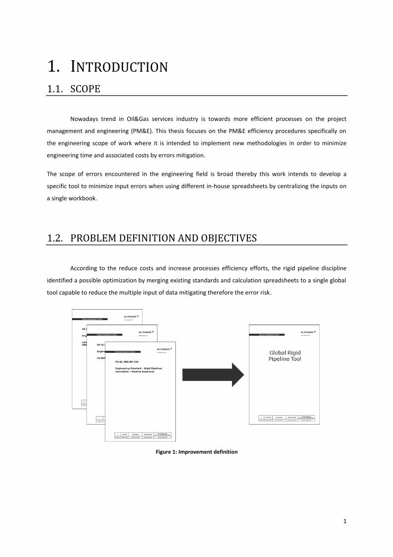
Figure 1: Improvement definition ........................................................................................................................... 1

Figure 2: Mechanical design philosophies, Source: Subsea 7 ................................................................................. 3

Figure 3: Link between design cases and limit states, Source: Ref. [1] ................................................................... 4

Figure 4: Example of Pipe burst, Source: Subsea 7 ................................................................................................. 5

Figure 5: Example of Pipe local collapse, Source: Subsea 7 .................................................................................... 6

Figure 6: Example of Propagating buckle, Source: Subsea 7................................................................................... 6

Figure 7: Buckle arrestor, Source: Subsea 7 ............................................................................................................ 7

Figure 8: Example of Local Buckling due to Combined Loads, Source: Subsea 7 .................................................... 7

Figure 9: Pipeline expansion loads, Source: Subsea 7 ............................................................................................. 8

Figure 10: Effective force distribution for short pipeline, Source: Subsea 7 ........................................................... 9

Figure 11: Effective force distribution for long pipeline, Source: Subsea 7 ............................................................ 9

Figure 12: Vertical Connector Jumper, Source: Subsea 7 ..................................................................................... 10

Figure 13: Example of Lateral Buckling, Source: Subsea 7 .................................................................................... 10

Figure 14: Pipeline loads on seabed, Source: Subsea 7 ........................................................................................ 12

Figure 15: Wall thickness definition, Source: Subsea 7 ......................................................................................... 14

Figure 16: Pressure definition, Source: Subsea 7 .................................................................................................. 14

Figure 17: Local pressure distribution, Source: Subsea 7 ..................................................................................... 15

Figure 18: Material de-rating, Source: Ref. [1] ...................................................................................................... 16

Figure 19: Coulomb friction force, Source: Subsea 7 ............................................................................................ 23

Figure 20: Peak enhancement factor, Source: Ref. [6] ......................................................................................... 27

Figure 21: Wave spreading function, Source: Ref. [4] ........................................................................................... 28

Figure 22: Global tool design modules workflow.................................................................................................. 37

Figure 23: Global tool user interface .................................................................................................................... 37

Figure 24: Trapezoidal Element, Source: Subsea 7 ............................................................................................... 38

Figure 25: Newton-Raphson Method, Source: Subsea 7 ...................................................................................... 39

Figure 26: Data Workflow ..................................................................................................................................... 40

Figure 27: Pipeline Coating Arrangement, Source: Subsea 7 ................................................................................ 42

Figure 28: Operational pressure and temperature ............................................................................................... 45

Figure 29: Bathymetry and seawater temperature .............................................................................................. 45

Figure 30: Validated Spreadsheet Result (left) and Global Tool Result (right) ..................................................... 54

Figure 31: Validated Spreadsheet Result (left) and Global Tool Result (right) ..................................................... 54

Figure 32: Validated Spreadsheet Result (left) and Global Tool Result (right) ..................................................... 55

Figure 33: JONSWAP Wave Spectrum from OrcaFlexTM

........................................................................................ 58

Figure 34: JONSWAP Spectrum from Global Tool ................................................................................................. 58

Figure 35: Validated Spreadsheet Result (left) and Global Tool Result (right) ..................................................... 59

x

xi

LIST OF TABLES

Table 1: Code wall thickness definition ................................................................................................................. 13

Table 2: Pipeline characteristics ............................................................................................................................ 41

Table 3: Steel properties ....................................................................................................................................... 42

Table 4: Anti-corrosion coating properties ........................................................................................................... 42

Table 5: Concrete weight coating properties ........................................................................................................ 43

Table 6: Operational and Environmental Data...................................................................................................... 43

Table 7: Wall thickness design loads ..................................................................................................................... 44

Table 8: Soil friction coefficients ........................................................................................................................... 44

Table 9: Lateral Buckling Additional Input Data .................................................................................................... 45

Table 10: Pipeline Route Characterization ............................................................................................................ 46

Table 11: Wave Spectrum ..................................................................................................................................... 46

Table 12: Cathodic protection design data ........................................................................................................... 46

Table 13: Coating breakdown factors ................................................................................................................... 47

Table 14: Anode geometrical characteristics ........................................................................................................ 47

Table 15: Pipeline Expansion Validation Cases ..................................................................................................... 48

Table 16: Lateral Buckling Screening Validation Cases ......................................................................................... 49

Table 17: DNV factors ........................................................................................................................................... 50

Table 18: DNV Wall Thickness Results .................................................................................................................. 51

Table 19: DNV Local Buckling Check ..................................................................................................................... 51

Table 20: API factors ............................................................................................................................................. 52

Table 21: API Wall Thickness Results .................................................................................................................... 52

Table 22: API Load Check ...................................................................................................................................... 53

Table 23: Pipeline Expansion PE.01 Validation Case Results ................................................................................ 53

Table 24: Pipeline Expansion PE.02 Validation Case Results ................................................................................ 54

Table 25: Pipeline Expansion PE.03 Validation Case Results ................................................................................ 55

Table 26: Lateral Buckling Screening LBS.01 Validation Case Results ................................................................... 56

Table 27: Lateral Buckling Screening LBS.02 Validation Case Results ................................................................... 56

Table 28: Lateral Buckling Screening LBS.03 Validation Case Results ................................................................... 57

Table 29: Spectral Analysis Results ....................................................................................................................... 57

Table 30: Cathodic Protection Results .................................................................................................................. 59

Table 31: Integration Method Refinement Assessment ....................................................................................... 60

xii

xiii

GLOSSARY Based on Subsea 7 Glossary

Design Pressure Max internal pressure during normal operation defined at a specific reference elevation.

Hydrotest Pressure Internal pressure applied to as laid pipeline system following installation and connection to check for leaks and check weld integrity.

Incidental Pressure Max pressure the pipe is designed to withstand during any incidental (i.e. temporary) operating situation, such as surge pressure or unintended shut-in pressure.

Line Pipe Welded or seamless pipe, available with the ends plain, beveled, grooved, cold expanded, flanged, or threaded; principally used to convey gas, oil, or water.

Long Pipeline Pipeline long enough to be restrained axially by the friction with the seabed.

Mill Test Pressure check used to test strength integrity of individual piping components (e.g. pipe, bends, connectors) during the FAT following fabrication and manufacture.

Short Pipeline Pipeline too short to be restrained axially by the friction with the seabed.

UOE Pipe fabrication process for welded pipes, expanded

xiv

xv

ACRONYMS

3LPE 3-Layer Polyethylene

API American Petroleum Institute

ALS Accidental Limit State

ASD Allowable Stress Design

CBF Coating Breakdown Factor

CPY Company

DNV Det Norske Veritas

ERW Electrical Resistance Welding

FAT Factory Acceptance Test

FJC Field Joint Coating

FLS Fatigue Limit State

ILT In-Line Tee

ISO International Organization for Standardization

JIP Joint Industry Project

KP Kilometric Point

LFRD Load and Resistance Factor Design

LP Line Pipe

LSD Limit State Design

MPP Mid-Point Potential

MSL Mean Sea Level

N/A Not Available or Applicable

O&G Oil and Gas

OS Offshore Standard

PE Polyethylene

PLET Pipeline End Termination

PM&E Project Management and Engineering

RP Recommended Practice or Rigid Pipeline

SAW Submerged Arc Welding

SLS Serviceability Limit State

SMYS Specified Minimum Yield Stress

SMTS Specified Minimum Tensile Stress

TRB Three Roll Bending

ULS Ultimate Limit State

WD Water Depth

xvi

xvii

SYMBOLOGY

Uppercase Latin

aA

Anode surface area

afA Anode final exposed surface area

cA Coated surface area

iA

Internal cross section area

oA

External cross section area

sA

Cross section area (corroded or not corroded)

B Attenuation constant

YC Peak horizontal load coefficient

ZC Peak vertical load coefficient

D Outer steel diameter

E Young’s modulus

aE Design closed circuit potential

xEa Anode potential function

cE Design protective potential

corrE Corrosion potential

YF Peak horizontal load

ZF Peak vertical load

H Residual lay tension

afI Final anode current output

xI a Anode current function

cmI Total mean current demand

cfI Total final current demand

ID Overall inner diameter

AttL Attenuated length

intjoL Joint or double Joint length

totalL

Total pipeline section length

xviii

M Minimum total anode mass

aM Mass of one anode

agM Gross mass of one anode

insM Insert material mass

totM Total anode mass required

tN

Number of tapers

aN

Number of anodes

iN Number of anodes per current criteria

mN Number of anodes per mass criteria

OD Overall outer diameter

afR Final anode resistance

LR Linear resistance

MeR

Steel resistivity

aP Incidental overpressure

bP Specified minimum burst pressure of pipe

cP Collapse pressure of pipe

dP Design pressure of the pipeline

eP Elastic collapse pressure

iP Internal pressure

oP External hydrostatic pressure

pP Buckle propagation pressure

tP Hydrostatic pressure

yP Yield pressure at collapse

S Specified minimum yield stress

T Sea state duration

T Single design oscillation derived period

aT

Axial tension (API)

maxT

Maximum operating temperature

pT Peak period

xix

swT

Seawater temperature

U Specified minimum tensile stress

agV Gross anode volume

pV Pocket (bolt recess) volume

tV Taper volume

WT Steel wall thickness

Lowercase Latin

a Combined coating breakdown constant

FJCa Field joint coating breakdown constant

LPCa Field joint coating breakdown constant

b Combined coating breakdown constant or buoyancy per unit length

FJCb Line pipe coating breakdown constant

LPCb Line pipe coating breakdown constant

d Inner steel diameter

0f Out of roundness

1f Bending safety factor for installation bending plus external pressure

2f Bending safety factor for in-place bending plus external pressure

cf Collapse factor for use with combined pressure and bending loads

df Internal pressure factor

ef Weld joint factor

of Collapse factor

pf Propagating buckle design factor

cbf Calculation variable

cmf Mean breakdown factor

cff Final breakdown factor

'

cff Mean final breakdown factor

tempyf , De-rating on yield stress

tempuf , De-rating on tensile stress

g Collapse reduction factor

h Water depth

xx

maxh Maximum water depth

minh Minimum water depth

refh Elevation at pressure reference level

cmi Design mean current density

g Gravity acceleration

bp Pressure containment resistance

cp Characteristics collapse pressure

dp Design pressure

ep External pressure

elp Elastic collapse pressure

incp Incidental pressure

lip Local incidental pressure

ltp Local system test pressure

minp Minimum internal pressure

pp Plastic collapse pressure

prp Propagating pressure

stp System test pressure

ytotr , Horizontal load reduction factor

ztotr , Vertical load reduction factor

ACCt Anti-corrosion coating thickness

CWCt Concrete weight coating thickness

coatt Overall coating thickness

corrt Corrosion allowance

nomt Nominal steel wall thickness

at Anode thickness

ft Design life

fabt Fabrication thickness tolerance

tt Anode end taper thickness

sw Submerged weight per unit length

xxi

Lowercase Greek

Thermal coefficient of expansion

fab Material fabrication factor

c Flow stress parameter

gw Girth weld factor

h Material hardening factor

spt System test pressure factor

p Pressure factor

U Material strength factor

Combined loading criteria factor

SC Safety class factor

A Accidental load factor

E Environmental load factor

inc Incidental to design pressure ratio factor

m Material resistance factor

W Vertical stability safety factor

Ovality

Electrochemical capacity

c Collapse strain

Sd Design strain

ax Axial friction coefficient

y Lateral friction coefficient

sw Seawater kinematic viscosity

Poisson ratio

Environmental resistivity

a Anode material density

ACC Anti-corrosion coating density

CWC Concrete weight coating density

cont Content density

xxii

s Steel density

t System test density (API)

st System test density

sw Seawater density

xxiii

UNITS SYSTEMS CONVERSION

Conventional System Units International System Units

1 bar 100 000 Pa

1 barg 100 000 Pa

1 bara 101 325 Pa

1’ (ft) 0.3048 m

1’’ (in) 0.0254 m

xxiv

1

1. INTRODUCTION 1.1. SCOPE

Nowadays trend in Oil&Gas services industry is towards more efficient processes on the project

management and engineering (PM&E). This thesis focuses on the PM&E efficiency procedures specifically on

the engineering scope of work where it is intended to implement new methodologies in order to minimize

engineering time and associated costs by errors mitigation.

The scope of errors encountered in the engineering field is broad thereby this work intends to develop a

specific tool to minimize input errors when using different in-house spreadsheets by centralizing the inputs on

a single workbook.

1.2. PROBLEM DEFINITION AND OBJECTIVES

According to the reduce costs and increase processes efficiency efforts, the rigid pipeline discipline

identified a possible optimization by merging existing standards and calculation spreadsheets to a single global

tool capable to reduce the multiple input of data mitigating therefore the error risk.

Figure 1: Improvement definition

2

The main objective of this dissertation is to develop this specific software tool for rigid pipeline design

considering the internal standards, international industry standards, best practices and lessons learned. The

objectives are summarized as follows:

Development of a specific software tool for rigid pipelines design;

Validation of the tool with project data;

Enrichment of the tool by considering multidisciplinary engineering best practices and lessons learned.

1.3. STRUCTURE OF THE DISSERTATION

This dissertation intends to perform a logical chain to describe the fundamentals of rigid pipeline

design, the standard design formulation, the implemented methodology and illustrative example based on

project data for validation.

Chapter 1 addresses the scope of the dissertation and its problem definition and objectives.

In Chapter 2 the fundamentals of design are summarized according to different international and industry

approved standards. It pretends to describe the main design premises for designing a marine pipeline.

In Chapter 3 pipeline design formulation is presented and the considerations and assumptions are scrutinized.

Chapter 4 focuses on the conceptual approach for the global tool development and solutions implemented

such as the numerical solver and the integration method.

Chapter 5 outlines the results and discussion of the software tool based on its deliverables and an illustrative

example based on project data validation scheme.

Finally Chapter 6 draws the conclusions and the key findings and proposes further developments.

Due to the large amount of information that references and supports this dissertation a References and

Appendix chapters are added.

3

2. FUNDAMENTALS OF RIGID PIPELINE DESIGN

In this chapter the fundamentals of rigid pipeline design are stated. The key design philosophies and

approaches for the preliminary pipeline design are endorsed herein.

2.1. MECHANICAL DESIGN

2.1.1. DESIGN PHILOSOPHIES

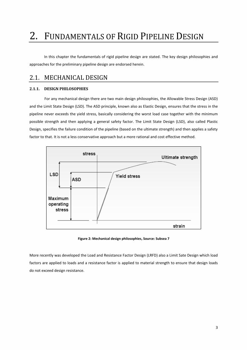
For any mechanical design there are two main design philosophies, the Allowable Stress Design (ASD)

and the Limit State Design (LSD). The ASD principle, known also as Elastic Design, ensures that the stress in the

pipeline never exceeds the yield stress, basically considering the worst load case together with the minimum

possible strength and then applying a general safety factor. The Limit State Design (LSD), also called Plastic

Design, specifies the failure condition of the pipeline (based on the ultimate strength) and then applies a safety

factor to that. It is not a less conservative approach but a more rational and cost effective method.

Figure 2: Mechanical design philosophies, Source: Subsea 7

More recently was developed the Load and Resistance Factor Design (LRFD) also a Limit Sate Design which load

factors are applied to loads and a resistance factor is applied to material strength to ensure that design loads

do not exceed design resistance.

4

2.1.2. DESIGN LIMIT STATES

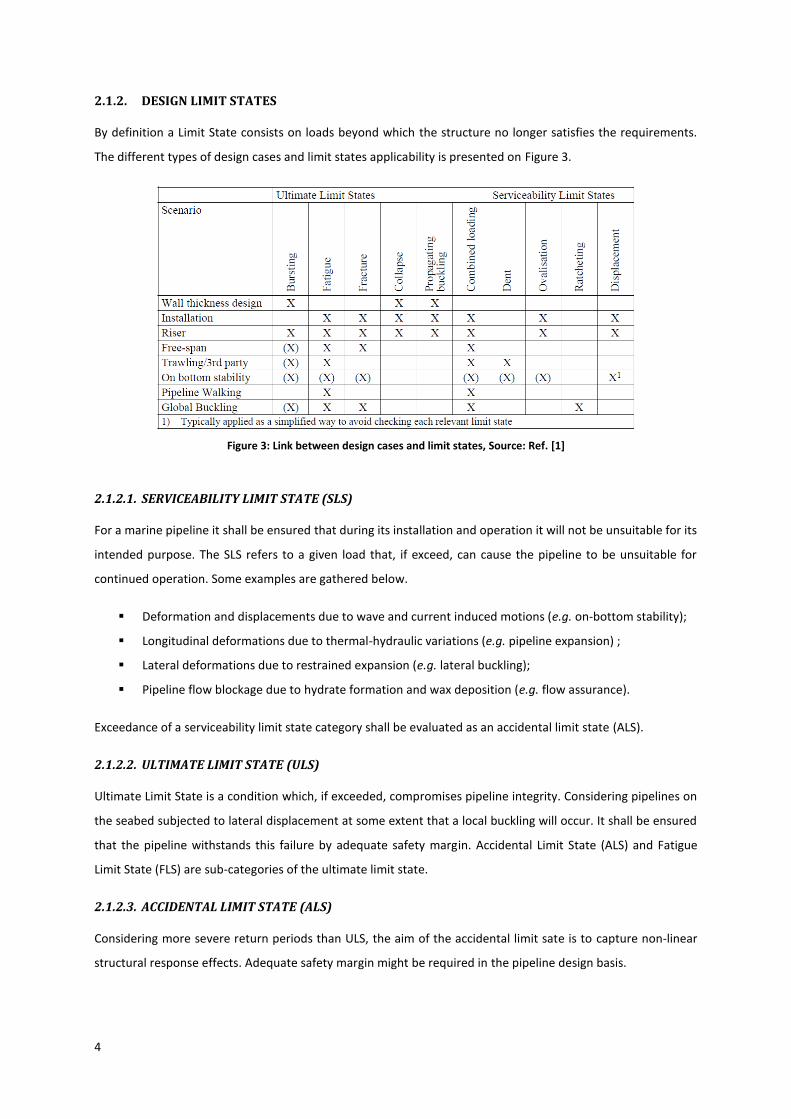
By definition a Limit State consists on loads beyond which the structure no longer satisfies the requirements.

The different types of design cases and limit states applicability is presented on Figure 3.

Figure 3: Link between design cases and limit states, Source: Ref. [1]

2.1.2.1. SERVICEABILITY LIMIT STATE (SLS)

For a marine pipeline it shall be ensured that during its installation and operation it will not be unsuitable for its

intended purpose. The SLS refers to a given load that, if exceed, can cause the pipeline to be unsuitable for

continued operation. Some examples are gathered below.

Deformation and displacements due to wave and current induced motions (e.g. on-bottom stability);

Longitudinal deformations due to thermal-hydraulic variations (e.g. pipeline expansion) ;

Lateral deformations due to restrained expansion (e.g. lateral buckling);

Pipeline flow blockage due to hydrate formation and wax deposition (e.g. flow assurance).

Exceedance of a serviceability limit state category shall be evaluated as an accidental limit state (ALS).

2.1.2.2. ULTIMATE LIMIT STATE (ULS)

Ultimate Limit State is a condition which, if exceeded, compromises pipeline integrity. Considering pipelines on

the seabed subjected to lateral displacement at some extent that a local buckling will occur. It shall be ensured

that the pipeline withstands this failure by adequate safety margin. Accidental Limit State (ALS) and Fatigue

Limit State (FLS) are sub-categories of the ultimate limit state.

2.1.2.3. ACCIDENTAL LIMIT STATE (ALS)

Considering more severe return periods than ULS, the aim of the accidental limit sate is to capture non-linear

structural response effects. Adequate safety margin might be required in the pipeline design basis.

5

2.1.2.4. FATIGUE LIMIT STATE (FLS)

It is defined as an ULS condition for cyclic load effects.

2.1.3. DESIGN LOADS

It is possible to classify marine pipeline loads as follows:

Functional Loads, resultant from the operation of the pipeline mainly, self-weight, content weights

and loads due to temperature/pressure variations;

Environmental Loads, defined as the interaction loads between the pipeline and the environment

mainly wave and current induced loads;

Accidental Loads, originated from natural hazards (earthquakes, mudslides, pockmarks) and third

party hazards (dropped objects, fishing activities);

Installation Loads covers all the loads due to installation and commission activities. These loads are

quantified prior to the operation by dedicated software and allowable sea states are defined for

specific acceptable limits.

Combination of Loads, as engineering principle for a design case the most unfavorable combination of

loads is taken into account.

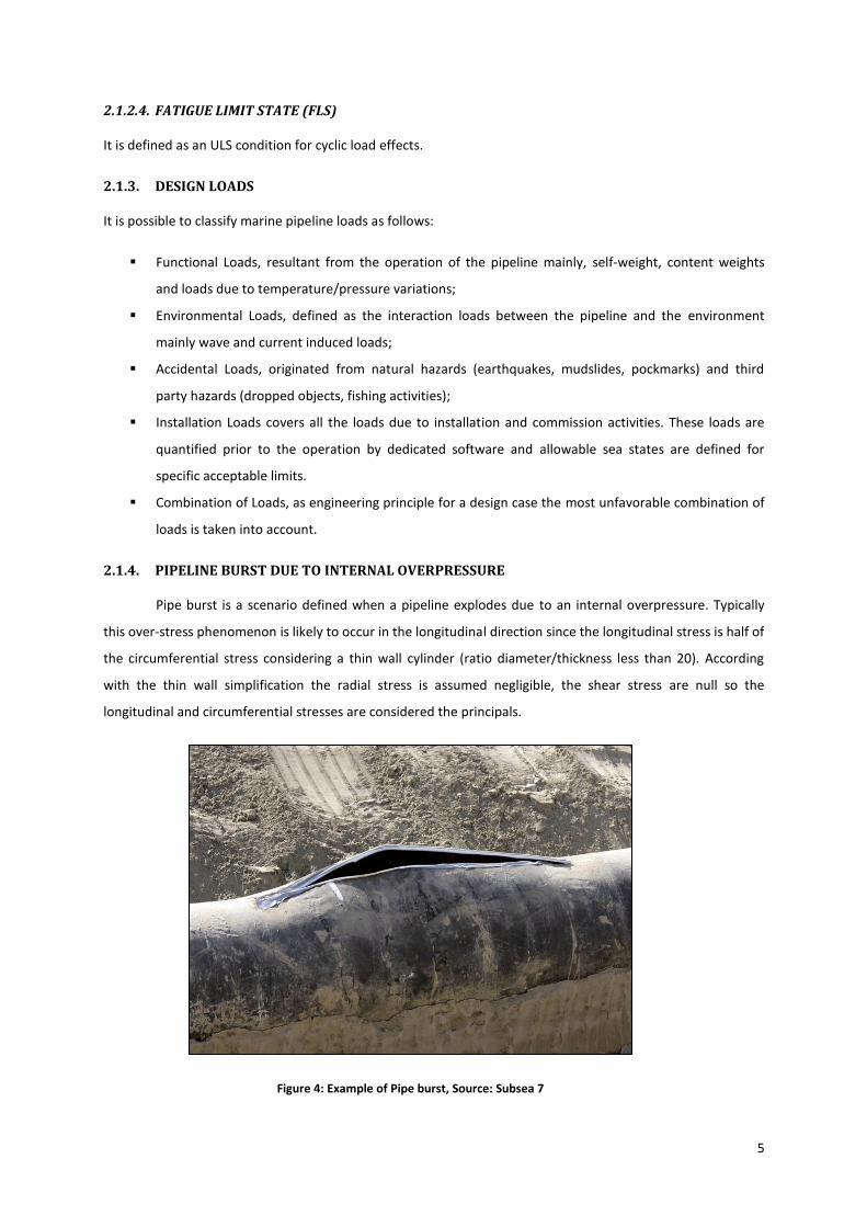
2.1.4. PIPELINE BURST DUE TO INTERNAL OVERPRESSURE

Pipe burst is a scenario defined when a pipeline explodes due to an internal overpressure. Typically

this over-stress phenomenon is likely to occur in the longitudinal direction since the longitudinal stress is half of

the circumferential stress considering a thin wall cylinder (ratio diameter/thickness less than 20). According

with the thin wall simplification the radial stress is assumed negligible, the shear stress are null so the

longitudinal and circumferential stresses are considered the principals.

Figure 4: Example of Pipe burst, Source: Subsea 7

6

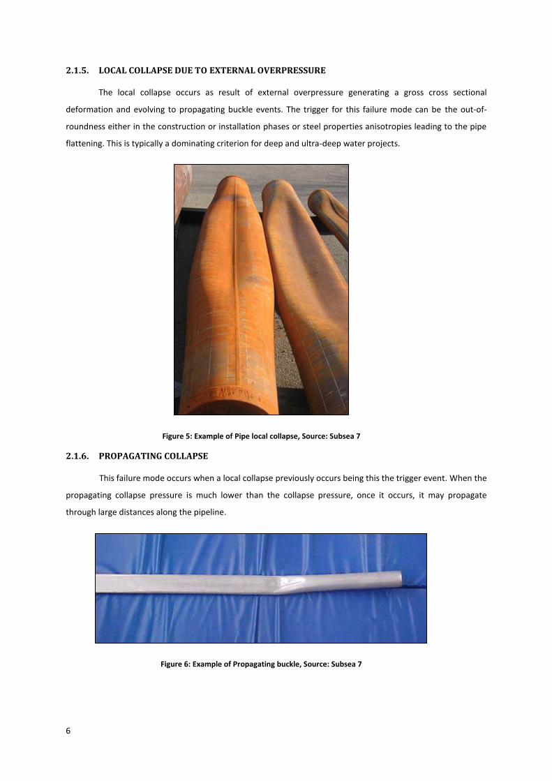
2.1.5. LOCAL COLLAPSE DUE TO EXTERNAL OVERPRESSURE

The local collapse occurs as result of external overpressure generating a gross cross sectional

deformation and evolving to propagating buckle events. The trigger for this failure mode can be the out-of-

roundness either in the construction or installation phases or steel properties anisotropies leading to the pipe

flattening. This is typically a dominating criterion for deep and ultra-deep water projects.

Figure 5: Example of Pipe local collapse, Source: Subsea 7

2.1.6. PROPAGATING COLLAPSE

This failure mode occurs when a local collapse previously occurs being this the trigger event. When the

propagating collapse pressure is much lower than the collapse pressure, once it occurs, it may propagate

through large distances along the pipeline.

Figure 6: Example of Propagating buckle, Source: Subsea 7

7

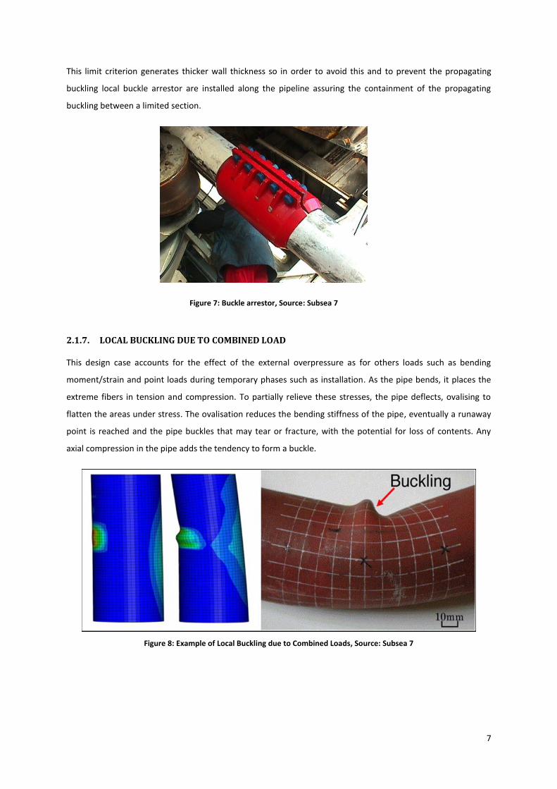
This limit criterion generates thicker wall thickness so in order to avoid this and to prevent the propagating

buckling local buckle arrestor are installed along the pipeline assuring the containment of the propagating

buckling between a limited section.

Figure 7: Buckle arrestor, Source: Subsea 7

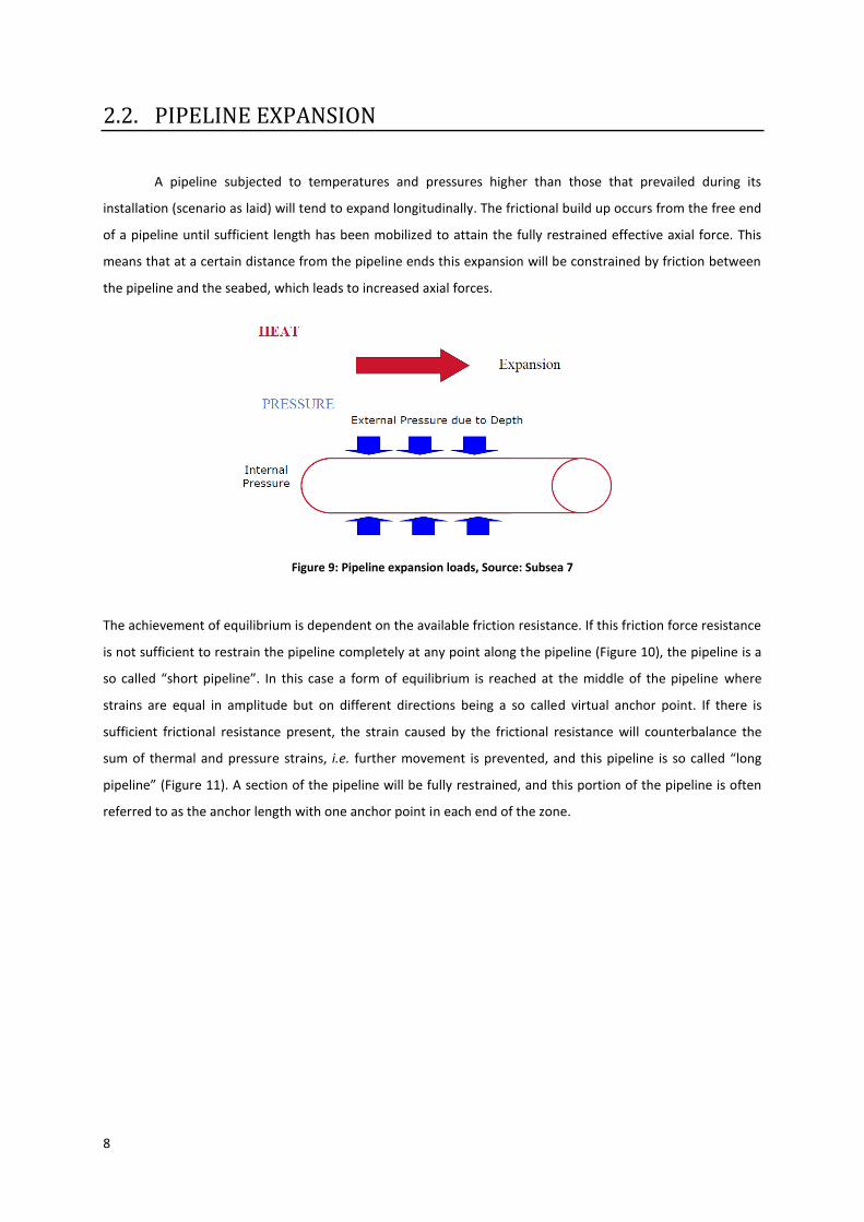
2.1.7. LOCAL BUCKLING DUE TO COMBINED LOAD

This design case accounts for the effect of the external overpressure as for others loads such as bending

moment/strain and point loads during temporary phases such as installation. As the pipe bends, it places the

extreme fibers in tension and compression. To partially relieve these stresses, the pipe deflects, ovalising to

flatten the areas under stress. The ovalisation reduces the bending stiffness of the pipe, eventually a runaway

point is reached and the pipe buckles that may tear or fracture, with the potential for loss of contents. Any

axial compression in the pipe adds the tendency to form a buckle.

Figure 8: Example of Local Buckling due to Combined Loads, Source: Subsea 7

8

2.2. PIPELINE EXPANSION

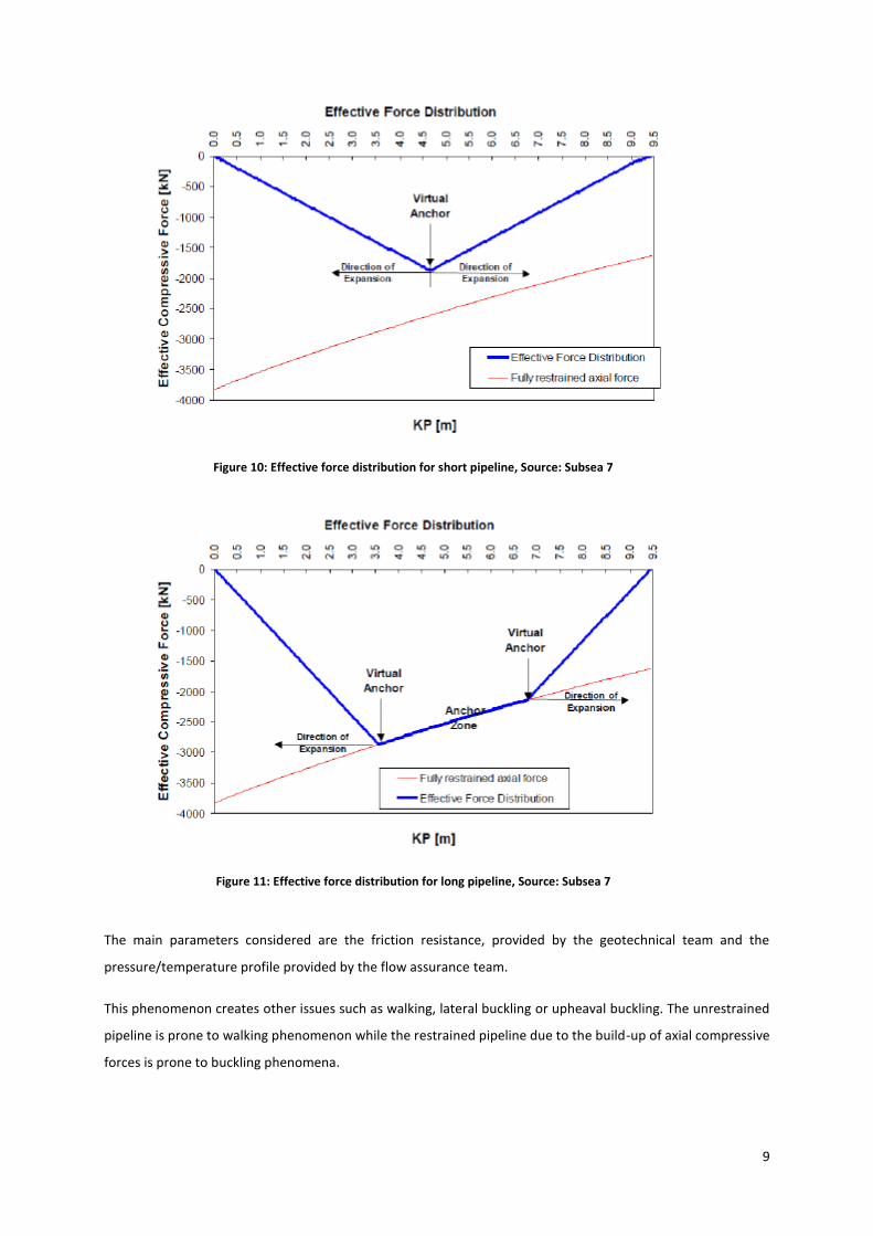
A pipeline subjected to temperatures and pressures higher than those that prevailed during its

installation (scenario as laid) will tend to expand longitudinally. The frictional build up occurs from the free end

of a pipeline until sufficient length has been mobilized to attain the fully restrained effective axial force. This

means that at a certain distance from the pipeline ends this expansion will be constrained by friction between

the pipeline and the seabed, which leads to increased axial forces.

Figure 9: Pipeline expansion loads, Source: Subsea 7

The achievement of equilibrium is dependent on the available friction resistance. If this friction force resistance

is not sufficient to restrain the pipeline completely at any point along the pipeline (Figure 10), the pipeline is a

so called “short pipeline”. In this case a form of equilibrium is reached at the middle of the pipeline where

strains are equal in amplitude but on different directions being a so called virtual anchor point. If there is

sufficient frictional resistance present, the strain caused by the frictional resistance will counterbalance the

sum of thermal and pressure strains, i.e. further movement is prevented, and this pipeline is so called “long

pipeline” (Figure 11). A section of the pipeline will be fully restrained, and this portion of the pipeline is often

referred to as the anchor length with one anchor point in each end of the zone.

9

Figure 10: Effective force distribution for short pipeline, Source: Subsea 7

Figure 11: Effective force distribution for long pipeline, Source: Subsea 7

The main parameters considered are the friction resistance, provided by the geotechnical team and the

pressure/temperature profile provided by the flow assurance team.

This phenomenon creates other issues such as walking, lateral buckling or upheaval buckling. The unrestrained

pipeline is prone to walking phenomenon while the restrained pipeline due to the build-up of axial compressive

forces is prone to buckling phenomena.

10

Due to the pipeline terminations expansion the PLET structures must accommodate this displacements by using

bendable pipes – spools or jumpers – being this an important input for the subsea structures project

engineering.

Figure 12: Vertical Connector Jumper, Source: Subsea 7

2.3. PIPELINE BUCKLING AND WALKING

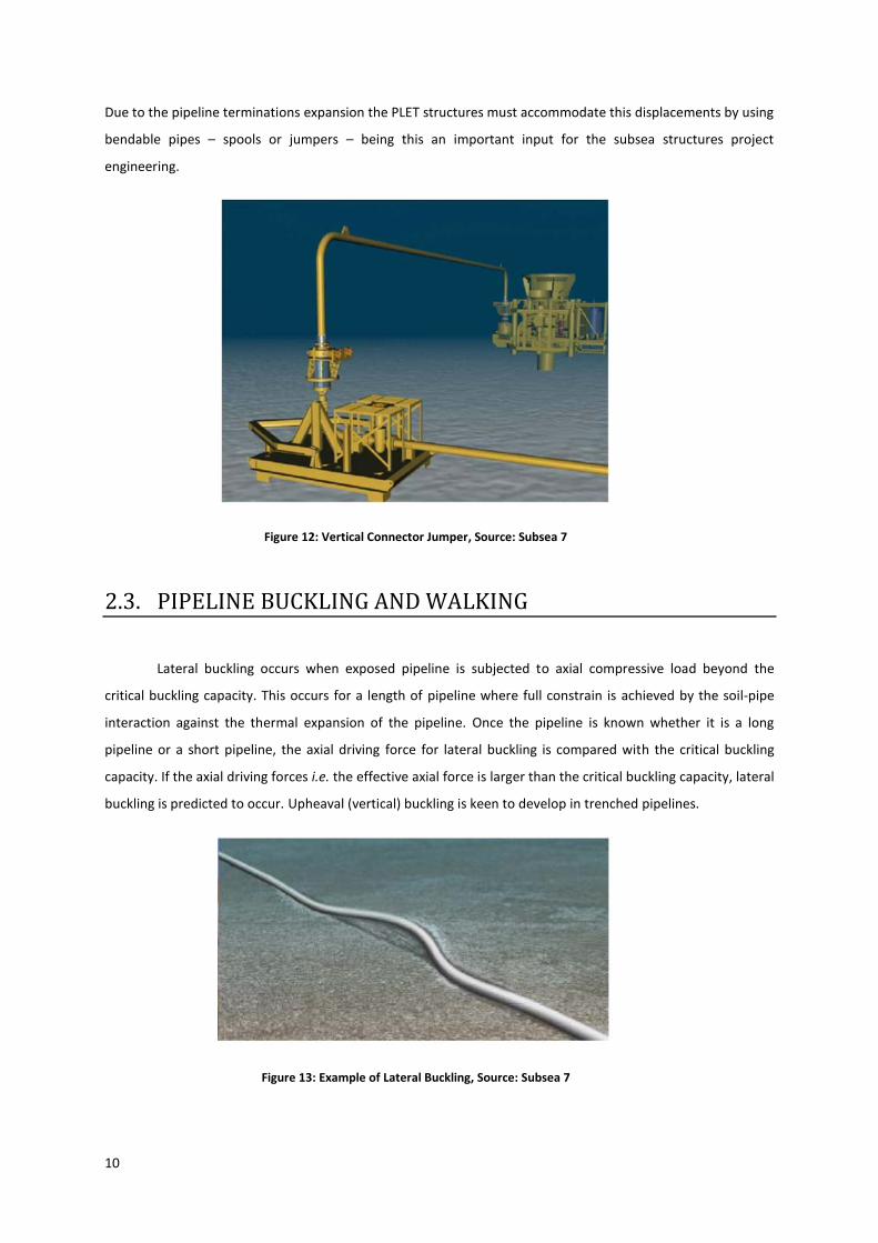
Lateral buckling occurs when exposed pipeline is subjected to axial compressive load beyond the

critical buckling capacity. This occurs for a length of pipeline where full constrain is achieved by the soil-pipe

interaction against the thermal expansion of the pipeline. Once the pipeline is known whether it is a long

pipeline or a short pipeline, the axial driving force for lateral buckling is compared with the critical buckling

capacity. If the axial driving forces i.e. the effective axial force is larger than the critical buckling capacity, lateral

buckling is predicted to occur. Upheaval (vertical) buckling is keen to develop in trenched pipelines.

Figure 13: Example of Lateral Buckling, Source: Subsea 7

11

Pipelines are subjected to thermal cycles along their service life which will induce expansions and contractions.

During the cool down process the pipeline will tend to contract although the frictional resistance will develop

and oppose the movement, thereby the pipeline will not walk back to its initial position leading to a global

displacement of the whole pipeline. In order for walking to occur, the pipeline or a section of the pipeline must

be unrestrained by soil friction, i.e. the axial restraint provided by the soil is insufficient to overcome the

loading due to pipeline loading. This phenomenon is difficult to assess as relies under uncertainties, although

the outcome can be substantially severe for the pipeline as:

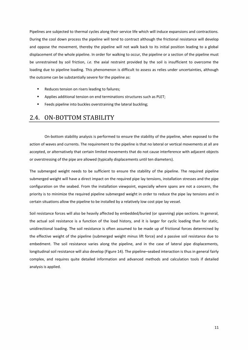
Reduces tension on risers leading to failures;

Applies additional tension on end terminations structures such as PLET;

Feeds pipeline into buckles overstraining the lateral buckling;

2.4. ON-BOTTOM STABILITY

On-bottom stability analysis is performed to ensure the stability of the pipeline, when exposed to the

action of waves and currents. The requirement to the pipeline is that no lateral or vertical movements at all are

accepted, or alternatively that certain limited movements that do not cause interference with adjacent objects

or overstressing of the pipe are allowed (typically displacements until ten diameters).

The submerged weight needs to be sufficient to ensure the stability of the pipeline. The required pipeline

submerged weight will have a direct impact on the required pipe lay tensions, installation stresses and the pipe

configuration on the seabed. From the installation viewpoint, especially where spans are not a concern, the

priority is to minimize the required pipeline submerged weight in order to reduce the pipe lay tensions and in

certain situations allow the pipeline to be installed by a relatively low cost pipe lay vessel.

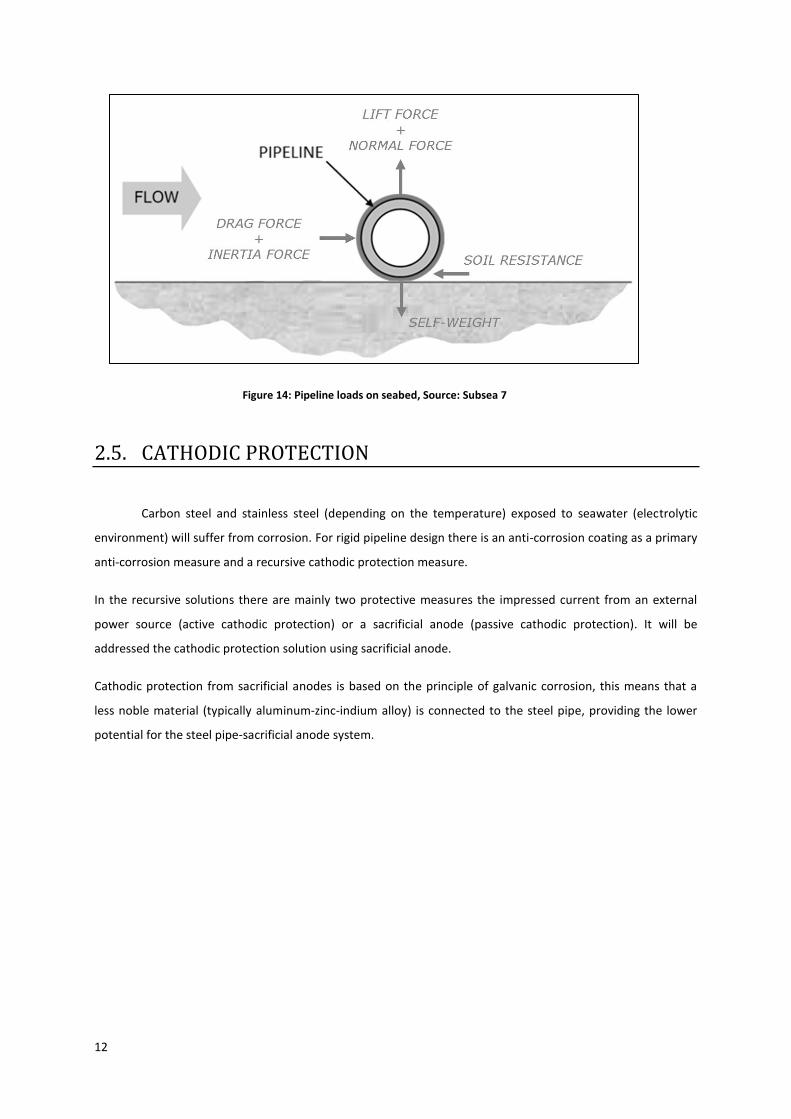
Soil resistance forces will also be heavily affected by embedded/buried (or spanning) pipe sections. In general,

the actual soil resistance is a function of the load history, and it is larger for cyclic loading than for static,

unidirectional loading. The soil resistance is often assumed to be made up of frictional forces determined by

the effective weight of the pipeline (submerged weight minus lift force) and a passive soil resistance due to

embedment. The soil resistance varies along the pipeline, and in the case of lateral pipe displacements,

longitudinal soil resistance will also develop (Figure 14). The pipeline–seabed interaction is thus in general fairly

complex, and requires quite detailed information and advanced methods and calculation tools if detailed

analysis is applied.

12

Figure 14: Pipeline loads on seabed, Source: Subsea 7

2.5. CATHODIC PROTECTION

Carbon steel and stainless steel (depending on the temperature) exposed to seawater (electrolytic

environment) will suffer from corrosion. For rigid pipeline design there is an anti-corrosion coating as a primary

anti-corrosion measure and a recursive cathodic protection measure.

In the recursive solutions there are mainly two protective measures the impressed current from an external

power source (active cathodic protection) or a sacrificial anode (passive cathodic protection). It will be

addressed the cathodic protection solution using sacrificial anode.

Cathodic protection from sacrificial anodes is based on the principle of galvanic corrosion, this means that a

less noble material (typically aluminum-zinc-indium alloy) is connected to the steel pipe, providing the lower

potential for the steel pipe-sacrificial anode system.

13

3. METHODOLOGY

Along this chapter rigid pipeline design formulation is addressed according to fundamentals stated on

the previous section.

3.1. MECHANICAL DESIGN

3.1.1. MECHANICAL DESIGN FOLLOWING DNV-OS-F101

3.1.1.1. INTRODUCTION

This offshore standard (Ref. [1]) gives the criteria and recommendations on concept development,

design, construction, operation and abandonment of submarine pipeline systems. This standard is based on

Limit State Design (LSD) philosophy specifically LFRD. The objectives of this standard are to:

Ensure that the concept, development, design, operation and abandonment of pipeline systems are

safe and conducted with regard to public safety and the protection of the environment;

Provide an internationally acceptable standard of safety for submarine pipeline systems by defining

minimum requirements for concept development, design, construction, operation and abandonment;

Serve as a technical reference document in contractual matters between Purchaser and Contractor;

Serve as a guideline for Designers, Purchaser and Contractors.

This module calculates the pressure containment resistance for installation and shut-down scenario, local

buckling (collapse) based on the external overpressure for installation and shut-down scenario and propagating

buckling based on the same assumption. At the end combined load check based on load controlled and

displacement controlled condition is performed.

3.1.1.2. WALL THICKNESS DEFINITION

Two different characterizations of the wall thickness are used; 1t and 2t are referred explicitly in the

design criteria. Thickness 1t is used where failure is likely to occur in connection with a low capacity (i.e.

system effects are present) while thickness 2t is used where failure is likely to occur in connection with an

extreme load effect at a location with average thickness.

Table 1: Code wall thickness definition

Code Wall Thickness Prior to Operation Operation

1t fabnom tt corrfabnom ttt

2t nomt corrnom tt

14

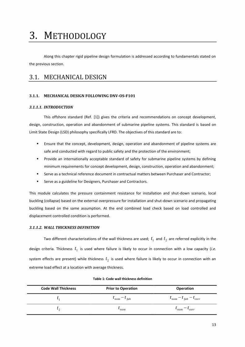
The fabrication tolerance is typically given as an absolute value or percentage of the nominal wall thickness

depending on the pipe manufacturing process (welded or seamless). The nominal wall thickness is therefore

calculated as:

fab

corrnom

t

ttt

%1

1

(1)

fabcorrnom tttt 1 (2)

The wall thickness definition is presented hereafter on Figure 15.

Figure 15: Wall thickness definition, Source: Subsea 7

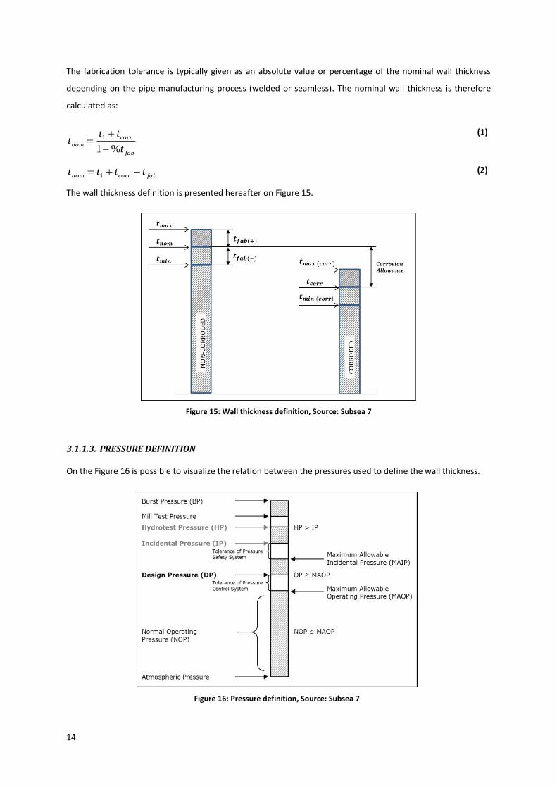
3.1.1.3. PRESSURE DEFINITION

On the Figure 16 is possible to visualize the relation between the pressures used to define the wall thickness.

Figure 16: Pressure definition, Source: Subsea 7

15

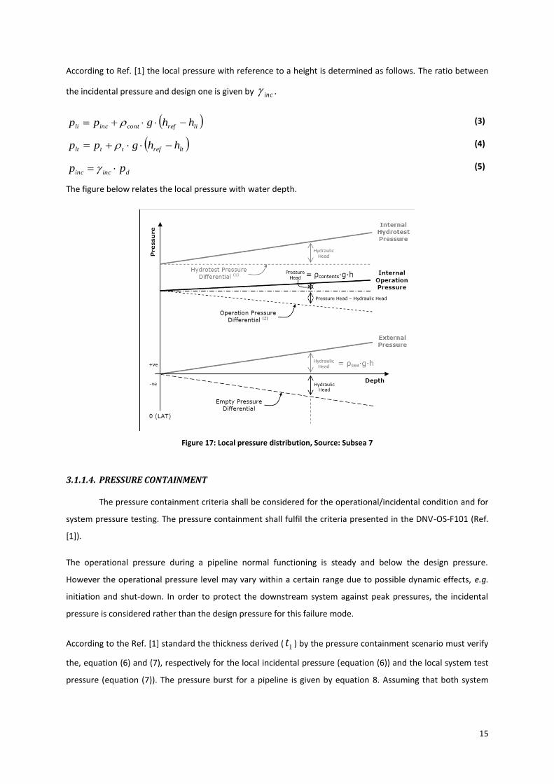
According to Ref. [1] the local pressure with reference to a height is determined as follows. The ratio between

the incidental pressure and design one is given by inc .

lirefcontincli hhgpp (3)

ltrefttlt hhgpp (4)

dincinc pp (5)

The figure below relates the local pressure with water depth.

Figure 17: Local pressure distribution, Source: Subsea 7

3.1.1.4. PRESSURE CONTAINMENT

The pressure containment criteria shall be considered for the operational/incidental condition and for

system pressure testing. The pressure containment shall fulfil the criteria presented in the DNV-OS-F101 (Ref.

[1]).

The operational pressure during a pipeline normal functioning is steady and below the design pressure.

However the operational pressure level may vary within a certain range due to possible dynamic effects, e.g.

initiation and shut-down. In order to protect the downstream system against peak pressures, the incidental

pressure is considered rather than the design pressure for this failure mode.

According to the Ref. [1] standard the thickness derived ( 1t ) by the pressure containment scenario must verify

the, equation (6) and (7), respectively for the local incidental pressure (equation (6)) and the local system test

pressure (equation (7)). The pressure burst for a pipeline is given by equation 8. Assuming that both system

16

pressure test and mill test pressure test have been performed according to Ref [1] the pressure containment

criteria shall be the governing one.

SCm

beli

tppp

1 (6)

SCm

belt

tppp

1 (7)

The burst pressure is given by the following equation and the thickness used can be both code wall thickness

according to the specification required and defined on Table 1,

3

22

cbb f

tD

ttp (8)

Where reduced material properties, cbf , are as follows,

15.1,min u

ycb

fff (9)

Utempyy fSMYSf ,

(10)

Utempuu fSMTSf ,

(11)

200100104.0

10050306.0

500

,,

TifT

TifT

Tif

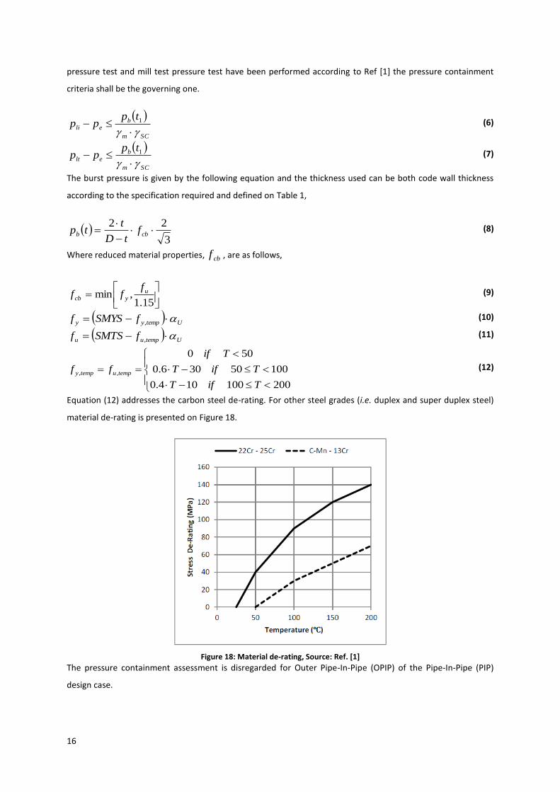
ff temputempy (12)

Equation (12) addresses the carbon steel de-rating. For other steel grades (i.e. duplex and super duplex steel)

material de-rating is presented on Figure 18.

Figure 18: Material de-rating, Source: Ref. [1]

The pressure containment assessment is disregarded for Outer Pipe-In-Pipe (OPIP) of the Pipe-In-Pipe (PIP)

design case.

17

3.1.1.5. LOCAL BUCKLING

Local buckling implies gross deformation of the cross section. The criterion is defined as follows.

SCm

ce

tppp

1

min (13)

The characteristics resistance for external pressure shall be calculated as:

t

Dftptptptptptptp pelcpcelc 0

22 (14)

The elastic and plastic resistance pressures are given as follows.

2

3

1

2

D

tE

tpel

(15)

D

tftp fabyp

2

(16)

The third degree polynomial equation has the following analytical solution.

bypc 3

1 (17)

Where:

tpb el (18)

t

Dftptptpc elpp 0

2 (19)

2tptpd pel (20)

cbu 2

3

1

3

1 (21)

dcbbv

3

1

27

2

2

1 3 (22)

3

1cosu

v (23)

180

60

3cos2

uy (24)

3.1.1.6. PROPAGATING BUCKLING

Propagation buckling cannot be initiated unless local buckling has occurred, the criterion given below.

SCm

pr

e

tppp

2

min (25)

18

Where:

5.2

2

2 35

D

tftp fabypr (26)

Valid on this range:

4515 2 tD

3.1.1.7. LOCAL BUCKLING DUE TO COMBINED LOADS

Load Controlled Condition (LCC)

A pipeline subjected to bending moment, effective axial force and internal overpressure shall verify

the following equation.

1

2

2

2

22

tp

pp

tS

pS

tM

M

bc

eip

pc

iSdSCm

pc

Sd

SCm

(27)

Valid on this range:

4.0

4515 2

pSd

ei

SS

pp

tD

A pipeline subjected to bending moment, effective axial force and external overpressure shall verify

the following condition.

1

2

2

min

2

22

tp

pp

tS

S

tM

M

cc

ep

pc

SdSCm

pc

Sd

SCm

(28)

That shall be considered valid on this range:

4.0

4515 2

pSd

ie

SS

pp

tD

The design loads are achieved as follows.

EEFFSd SSS (29)

EEFFSd MMM (30)

19

Displacement Controlled Condition (DCC)

A pipeline subjected to longitudinal compressive strain due to bending moment and effective axial

force and internal overpressure shall verify the following condition.

ec

Sd

ppt min2 ,

(31)

This shall be considered valid on the following range.

ei pp

tD

452

Where the design strain is given by:

EEFFSd (32)

The collapse strain is calculated as follows.

gwh

b

eec

tp

pp

D

tppt

5.1min

min 75.5101.078.0, (33)

A pipeline subjected to longitudinal compressive strain due to bending moment and effective axial force and

external overpressure shall verify the following condition.

1

0, 2

min

8.0

2

SCm

c

e

c

Sd

tp

pp

t

(34)

Shall be considered valid on this range.

epp

tD

min

2 45

3.1.1.8. BUCKLE ARRESTOR DESIGN

An integral buckle arrestor may be designed according to Ref. [1]:

SCm

X

e

pp

1.1 (35)

Where the crossover pressure is,

2

2

, 201D

LtEXPpppp BA

prBAprprX (36)

20

The propagating buckle capacity of an infinite arrestor is calculated with the buckle arrestor properties as

follows.

5.2

,2

,,,2, 35

BA

BA

BAfabBAyBABAprD

tftp (37)

3.1.2. MECHANICAL DESIGN FOLLOWING API-RP-1111

This recommended practice (Ref. [2]) sets criteria for the design, construction, testing, operation, and

maintenance of offshore steel pipelines utilized in the production, production support, or transportation of

hydrocarbons. This standard follows the Limit State Design (LSD) philosophy.

3.1.2.1. INTERNAL PRESSURE DESIGN

The design criteria are stated below.

btedt PfffP (38)

td PP 80.0 (39)

ta PP 90.0 (40)

Where tP is the hydrostatic test pressure, dP is the design pressure and aP is the accidental pressure. The

design factor ( df ), weld joint factor ( ef ) and the temperature de-rating factor ( tf ) are given as per Ref. [2].

The specified minimum burst pressure is given by:

i

bD

DUSP ln45.0 (41)

The internal pressure design is disregarded for Outer Pipe-In-Pipe (OPIP) of the Pipe-In-Pipe (PIP) design case.

Longitudinal Load Design

The effective tension, effT , due to static primary longitudinal loads shall not exceed the following criteria:

yeff TT 60.0 (42)

sy AST (43)

Combined Load Design

The combination of primary longitudinal load and differential pressure load shall not exceed that given by the

following equations respectively for operation (equation (44)), accidental and system test scenarios (equation

(45)).

21

90.0

22

y

eff

b

oi

T

T

P

PP (44)

96.0

22

y

eff

b

oi

T

T

P

PP (45)

3.1.2.2. EXTERNAL PRESSURE DESIGN

Collapse due to External Pressure

The following condition shall be verified.

ioco PPPf (46)

The collapse factor, of , and the collapse pressure is given by:

22

ey

ey

c

PP

PPP

(47)

Where the yield pressure and elastic pressure are provided respectively by,

D

tSPy 2 (48)

2

3

12

D

t

EPe

(49)

Buckling due to Combined Bending and External Pressure

Combined bending strain and external pressure load shall verify the following statement,

g

Pf

PP

cc

io

b

(50)

Where b is the buckling strain under pure bending and the collapse reduction factor as function of the ovality

is given by,

201

1g (51)

And to avoid buckling bending strains should be limited as follows:

11 f (52)

22 f (53)

22

Where 1 and 2 are respectively the maximum installation and in-place strains. The 1f and 2f are bending

safety factors.

Propagating Buckles

Buckle arrestors shall be used under the following condition,

ppio PfPP (54)

Where the propagating pressure is given by:

4.2

24

D

tSPp

(55)

23

3.2. PIPELINE EXPANSION

The fully restrained effective axial force is applied on the pipeline and is given by the following equation.

oisiires TTEAApHS 21 (56)

The axial friction force given by Coulomb approach is the following.

xwS axsff (57)

The effective axial force is given by the minimum between friction and fully restrained forces.

resffeff SSS ,min (58)

If the fully restrained force is higher than the friction force along the entire flowline there is no anchored

length.

It is defined a hot end where temperatures and pressures are higher and cold end at the other extremity. The

virtual anchored point from hot end is defined on the intersection between the fully restrained and friction

force if there is an anchored length, otherwise it will be considered at maximum friction point. The slope is

taken into account by achieving an equivalent friction coefficient.

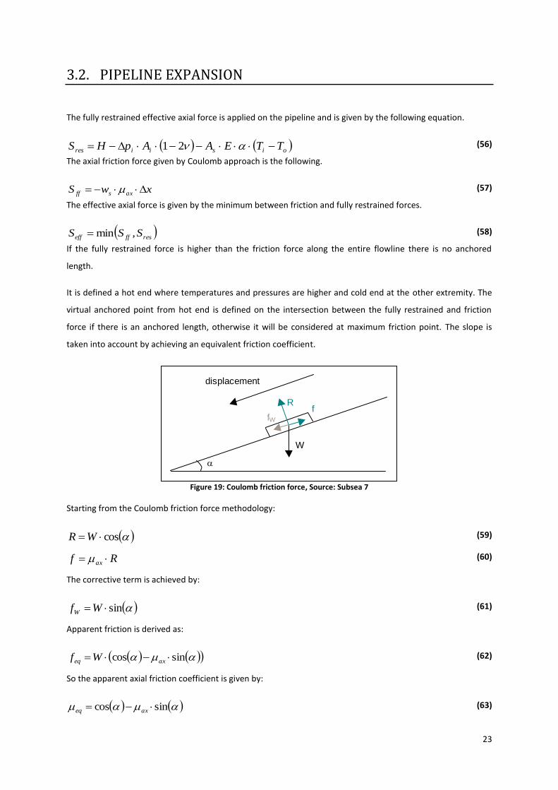
Figure 19: Coulomb friction force, Source: Subsea 7

Starting from the Coulomb friction force methodology:

cosWR (59)

Rf ax (60)

The corrective term is achieved by:

sinWfW (61)

Apparent friction is derived as:

sincos axeq Wf (62)

So the apparent axial friction coefficient is given by:

sincos axeq (63)

Rf

displacement

W

fW

24

The hot end, cold end and ILT expansion is then determined by,

dx

AE

xSxS

hotx s

ffres

hot

0

(64)

dx

AE

xSxScold

tot

x

L s

ffres

cold

(65)

dx

AE

xSxSILT

anchor

x

x s

ffres

ILT

(66)

There will be expansion at ILT if it’s positioned on the mobilized part of the pipeline.

3.3. LATERAL BUCKLING AND WALKING SCREENING

3.3.1. DESIGN CRITERIA

As per Ref. [3] the pipeline is susceptible to buckling if the following inequality is true:

Creff SS max, (67)

3.3.2. BUCKLING PHENOMENA

The critical buckling force is achieved by the following equation.

CrBcr SSS ,65.0min (68)

And relies on two parameters, one dependent of Euler buckling of straight pipeline section and other related to

pipeline curve sections. The critical force under which a buckle in a large radius route bend can be developed is

given by:

RSS LBcrB (69)

Where LBS is the maximum lateral friction force.

The Hobbs safe force for infinite mode buckling (based on Euler buckling) is given by:

21

80.3

D

SEIS LB (70)

25

3.4. ON-BOTTOM STABILITY

3.4.1. VERTICAL STABILITY

In order to avoid floatation in water, the submerged weight of the pipelines is checked to see if the

following criterion is met:

00.1

bw

b

s

W (71)

3.4.2. ABSOLUTE LATERAL STATIC STABILITY

The absolute lateral stability approach detailed in Ref. [4], restricts lateral displacement of pipeline, i.e.

hydrodynamic stability during a given sea state.

This is based on a static equilibrium of forces that ensures that the resistance of the pipe against motion is

sufficient to withstand maximum hydrodynamic loads during a sea state, i.e. the pipe will experience no lateral

displacement under the design extreme single wave induced oscillatory cycle in the sea state considered. The

following conditions shall be fulfilled:

00.1

Rssw

ZswY

SCFw

FF

(72)

00.1

s

ZSC

w

F (73)

Being the peak horizontal and vertical loads defined as:

2,2

1 VUCODrF YswytotY (74)

2,2

1 VUCODrF ZswztotZ (75)

The soil passive resistance force RF is defined either for sand or clay soils. Load reduction factor totr is

defined by the sum of reduction factors due to soil penetration, trenching and permeable seabed.

26

3.4.3. WAVE SPECTRA

3.4.3.1. JONSWAP SPECTRUM

The JONSWAP (Joint North Sea Wave Project) spectrum is formulated as a modification of the Pierson-

Moskowitz spectrum for a developing sea state in a fetch limited situation.

2

5.0expp

p

PMJ SAS

(76)

Being A a normalization factor.

ln287.01 A (77)

Since the Pierson-Moskowitz spectrum is given by:

4

542

4

5exp

16

5

p

psPM HS

(78)

The extended formulation of the JONSWAP spectrum is given below:

2

5.0exp4

52

4

5exp

p

p

p

J gS

(79)

Alpha is a parameter that relates to the wind speed and fetches length, otherwise is the intensity of the

spectra. Gamma is defined as peak enhancement factor and beta is the shape factor. According to Ref. [5] the

parameters are as follow:

ln287.0116

52

42

g

H ps (80)

else

p

09.0

07.0 (81)

0.50.1

0.56.315.175.5exp

6.30.5

s

p

s

p

s

p

s

p

H

T

H

T

H

T

H

T

(82)

Typical default values for the North Sea are the following.

25.1

3.3

01.0,0081.0

27

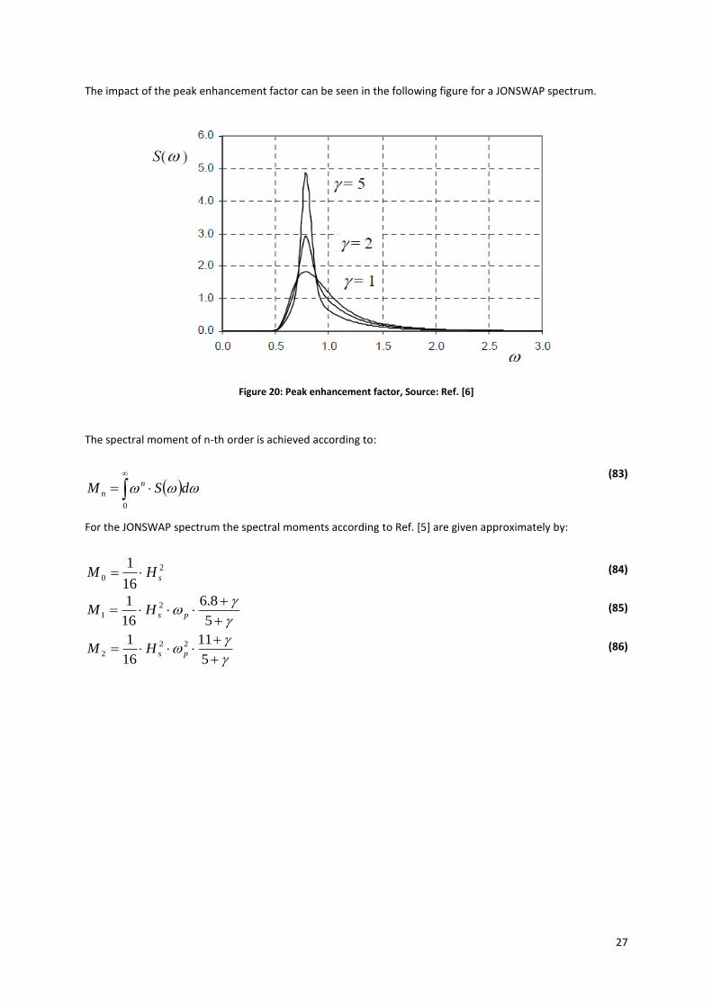
The impact of the peak enhancement factor can be seen in the following figure for a JONSWAP spectrum.

Figure 20: Peak enhancement factor, Source: Ref. [6]

The spectral moment of n-th order is achieved according to:

0

dSM n

n

(83)

For the JONSWAP spectrum the spectral moments according to Ref. [5] are given approximately by:

2

016

1sHM (84)

5

8.6

16

1 2

1 psHM (85)

5

11

16

1 22

2 psHM (86)

28

3.4.3.2. OCHI-HUBBLE SPECTRUM

Ochi and Hubble (Ref. [6]) suggested to describe bimodal spectra by a superposition of two modified

Pierson-Moskovitz spectra defined as a sum of two three-parameter wave spectra one representing the low

frequency components and the other high frequency components of the wave energy. The formulation is given

below.

2

1

4

14

2

4

14exp

4

14

4

1

j

mjjsj

j

mj

j

OHj

j

HS

(87)

For sake of simplicity within the tool it is defined only a single modal spectrum therefore the equation reduces

to:

4

14

2

4

14exp

4

14

4

1

ps

p

OH

HS

(88)

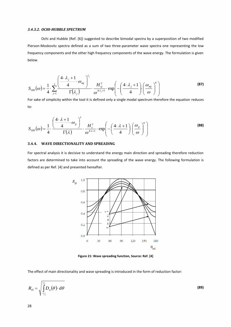
3.4.4. WAVE DIRECTIONALITY AND SPREADING

For spectral analysis it is decisive to understand the energy main direction and spreading therefore reduction

factors are determined to take into account the spreading of the wave energy. The following formulation is

defined as per Ref. [4] and presented hereafter.

Figure 21: Wave spreading function, Source: Ref. [4]

The effect of main directionality and wave spreading is introduced in the form of reduction factor:

2

2

dDR wD (89)

29

Where:

else

s

s

D w

s

w

0

22sincos

25.0

211 2

(90)

And the spreading factor:

else

s w

24

3

48

(91)

3.4.5. SPECTRAL ANALYSIS

The wave induced velocity spectrum at seabed may be obtained through a spectral transformation of the

waves at sea level using a first order wave theory.

SGSUU 2

(92)

The transfer function that transforms sea surface elevation to seabed wave induced velocity is given by:

hk

G

sinh

(93)

The dispersion relation, this is the relation between the wave frequency and wave number is given by a

transcendental equation:

hkkg

tanh2

(94)

There are some simplifications for shallow and deep water cases. For shallow water, defined as below the wave

number is given by:

hkh

2020

And for deep water:

hkh

2

Where the wavelength relation with wave number is,

k

2 (95)

30

For shallow water the relation between wave number and wave frequency reduces to:

hg

khkhk

tanh (96)

And for deep water:

g

khk2

1tanh

(97)

For all other case a numerical solver will solve the dispersion relation.

The spectral derived mean zero up-crossing period is given below.

2

02M

MTu (98)

The spectral derived oscillatory velocity is,

02 MU s (99)

The perpendicular projected single oscillation velocity amplitude is provided by.

Ds RUU

ln2

5772.0ln2

2

1 (100)

3.4.6. CURRENT ANALYSIS

The mean perpendicular current velocity over a pipe diameter is defined as:

c

r

rcc

z

z

z

OD

OD

z

zVVV sin

1ln

11ln1

0

0

0

*

(101)

31

3.5. CATHODIC PROTECTION

3.5.1. DESIGN CRITERIA

To meet anode mass criteria the following inequality shall be verified.

totaa MMN (102)

And to meet the final current output criteria the expression below shall be verified.

cfafa IIN (103)

According to Ref. [7] for distances between anodes higher than 300 m the effect of the metallic resistance in

the pipe wall shall be taken into account, for that anodes spacing larger than 300 m shall verify the attenuation

criteria.

For the attenuation criteria two formulations were implemented, the conservative DNV approach (Ref. [7]) and

a more realistic Uhlig’s approach (Ref. [8]).

According to Ref. [7] approach the protected length is as follows.

00

2

22

'

242. ac

cfcmMe

total

cfaf

total

cfaf

cmcfMe

Att EEWTDWT

Dfi

L

IR

L

IR

ifD

WTDWTL

(104)

The Uhlig’s approach (Ref. [8]) is presented below.

L

af

L

af

corr

acorr

corr

acorr

R

BR

R

BR

E

EE

E

EE

BL

1

18.08.0

ln2

22

max

(105)

Where the pipeline attenuation constant is,

cm

ccorr

cfL

i

EE

fRDB

'

(106)

The linear resistance is,

22 24

WTDD

RR Me

L

(107)

32

3.5.2. ANODE DESIGN

Based on typical project specifications it is defined two possible arrangements: combined breakdown factor

typically given by the ISO standard (Ref. [9]) and an individual breakdown for the Field Joint Factor (FJC) and

Line Pipe Coating (LPC) factor typically based on Ref. [7].

For that mean current demand is achieved for the FJC plus LPC currents or for the entire pipeline, taking into

account the surface coated areas.

cmLPCcmLPCcLPCcm ifAI .,, (108)

cmFJCcmFJCcFJCcm ifAI ,,, (109)

FJCcmLPCcmcm III ,, (110)

Or based in combined pipeline coating breakdown factor.

cmcmccm ifAI (111)

Where the mean coating breakdown factors are given for the combined arrangement as,

fcm tbaf 5.0 (112)

Or based on an individual arrangement,

fLPCLPCLPCcm tbaf 5.0, (113)

fFJCFJCFJCcm tbaf 5.0, (114)

The final coating breakdown is achieved following,

fLPCLPCLPCcf tbaf , (115)

fFJCFJCFJCcf tbaf , (116)

Or,

fcf tbaf (117)

The mean final coating breakdown factor is achieved by:

FJCcf

jo

FJCLPCcfcf f

L

Lff ,

int

,

' (118)

Final current demand is determined as follow:

cmLPCcfLPCcLPCcf ifAI .,, (119)

cmFJCcfFJCcFJCcf ifAI ,,, (120)

FJCcfLPCcfcf III ,, (121)

33

Or considering a combined arrangement,

cmcfccf ifAI (122)

The gross anode volume is determined by subtracting from a gross cylindrical anode volume the taper volume

and the bolt recess volume (pocket volume) and the inserted material volume.

ppttttaaaaaaag VNVNLNLhtdtdV

22

4

22 (123)

The pocket (bolt recess) volume is considered as follow.

3000125.0 mVp

And the tapered volume (truncated cone) is,

attatta

ta

t

ta

taata

ta

taaaat

hLthLtt

Ld

Ltt

Ltdtd

tt

LtdtdV

22

4

2

2

4

2

32

2

4

2

3

2

22

(124)

The gross anode mass is computed by multiplying the anode volume by its density.

agaag VM (125)

The insert material mass is considered 10 % of the gross anode mass.

agins MM 10.0

The net anode mass is therefore:

insaga MMM (126)

The total net anode mass to meet mean current demand is calculated as,

u

tIM

fcm

tot

8760 (127)

The anode final resistance according to Ref. [9] is given by,

af

afA

R

315.0 (128)

The final anode current output is given by,

34

af

ac

afR

EEI

(129)

The number of anodes based on mass criteria is given by.

a

tot

mM

MN (130)

The number of anodes based on the current criteria is given by.

af

cf

iI

IN (131)

Therefore maximum anode spacing, based on number of joints is given by,

imjo

tot

NNL

LS

,maxint

int

1 (132)

The maximum anode spacing, in meters is given by,

int12 joLSS (133)

The minimum number of anodes is given,

1int2

S

LN tot

a (134)

Therefore the total anode mass is achieved by,

aa MNM (135)

The current demand and potential required at the star of the protected pipeline is given by,

af

L

acorr

a

RL

BB

LBR

EEI

2sinh

2cosh

1

(136)

2sinh

2sinh

12L

B

LLB

II aa (137)

The end flowline electrochemical potential is given by,

11 aafaa IREE (138)

35

22 aafaa IREE (139)

Therefore the Mid-Point Potential (MPP) is given by,

2sinh

1

LBB

IRMPP a

L

(140)

The equation that provides the potential attenuation along the pipeline is given by,

corrEL

xBMPPxE

2cosh (141)

36

4. SOFTWARE TOOL DEVELOPMENT

In this chapter the conceptual design approach is scrutinized as the implemented solutions. The data

workflow is presented and the interaction between design modules is explained. The data for validation is

presented herein.

4.1. CONCEPTUAL DESIGN

The tool is developed towards an increasing process efficiency this is, avoiding multiple inputs typing

and therefore mitigating the error. It is also important to increase the interchangeability of data originated

from multiple modules. The end users target is the pipeline design engineers, therefore engineering judgment

is required.

Engineering tools are developed to minimize the time consumed by large number of repetitive calculations that

needs to be performed, although they need to be user-centered, pragmatic, accessible and clearly explained.

The application is developed in Microsoft™ Excel® using the Visual Basic for Applications (VBA) a powerful and

available tool. For simple calculations the standard Excel formulae database is used while for dedicated

applications VBA is applied, for instance in the case of spectral analysis.

4.1.1. MODULAR DESIGN AND DECISION PROCESS

The modular design approach enables further developments of the tool by independently adding new

design modules. This is a critical design criterion since the industry standards are continuously evolving and

incorporating field-proven methods.

The decision process aimed to a logic loop starting on the design and subsequent verification with pipeline

environmental and operational conditions known as in-place analysis. The process can be described as a

primary design, focusing wall thickness and buckle arrestor design, complementary design addressed by the

cathodic protection and design verification assessment by in-place analysis such as pipeline expansion, lateral

buckling screening and on-bottom stability. Consecutive loops of this process enable to define the pipeline, the

coating and the ancillary designs. This modular design approach enables the end user to run sequentially the

modules or execute individually each module.

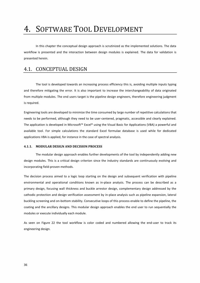
As seen on Figure 22 the tool workflow is color coded and numbered allowing the end-user to track its

engineering design.

37

Figure 22: Global tool design modules workflow

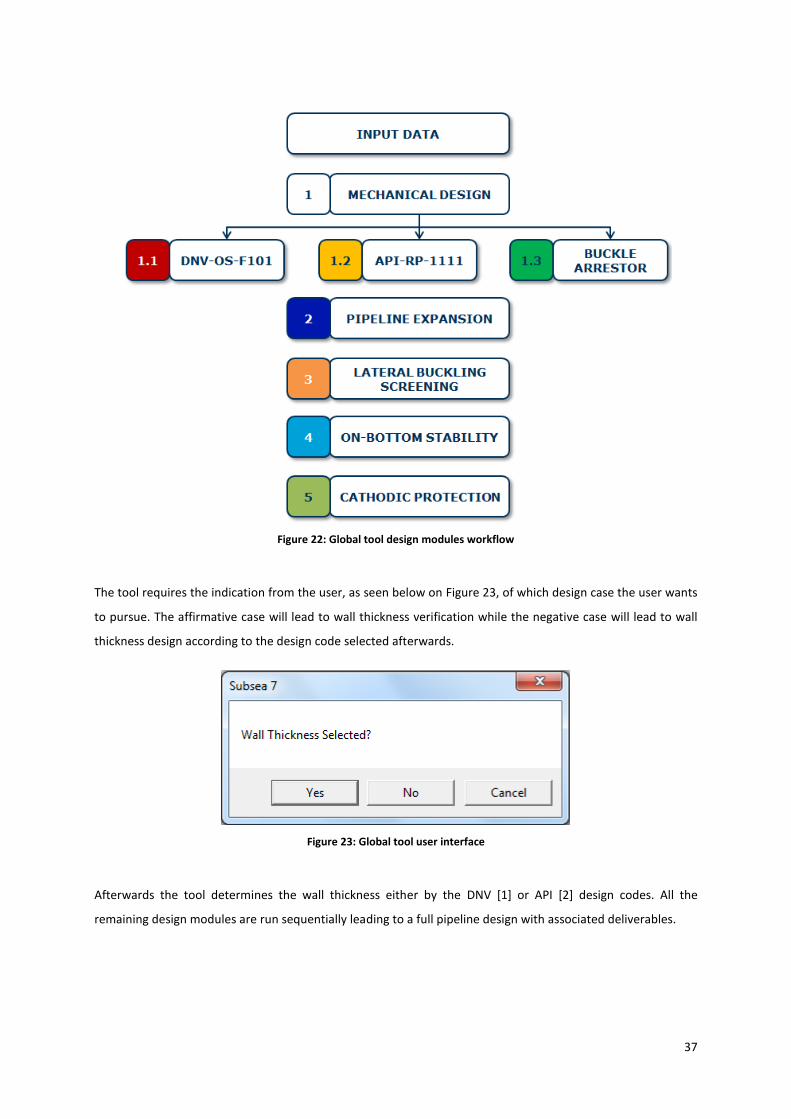
The tool requires the indication from the user, as seen below on Figure 23, of which design case the user wants

to pursue. The affirmative case will lead to wall thickness verification while the negative case will lead to wall

thickness design according to the design code selected afterwards.

Figure 23: Global tool user interface

Afterwards the tool determines the wall thickness either by the DNV [1] or API [2] design codes. All the

remaining design modules are run sequentially leading to a full pipeline design with associated deliverables.

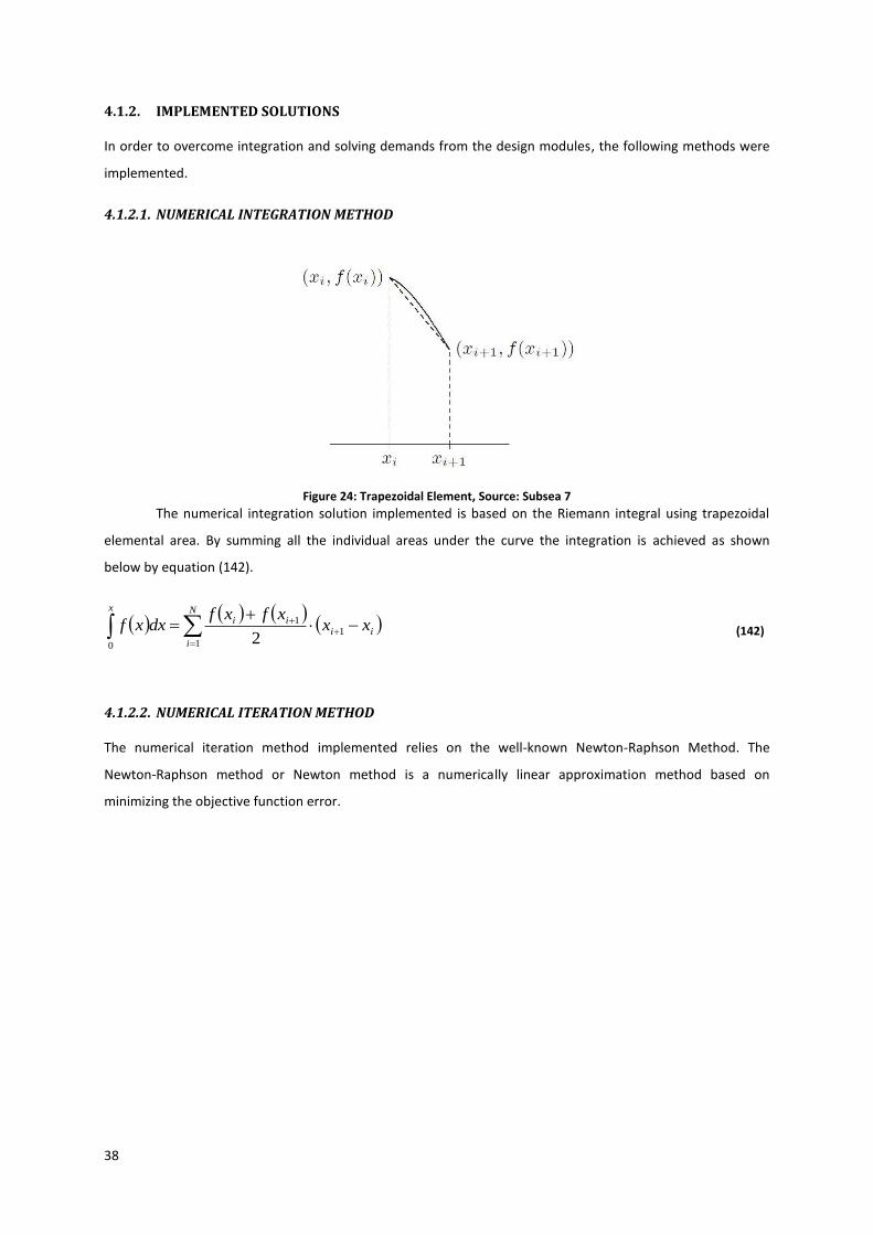
38

4.1.2. IMPLEMENTED SOLUTIONS

In order to overcome integration and solving demands from the design modules, the following methods were

implemented.

4.1.2.1. NUMERICAL INTEGRATION METHOD

The numerical integration solution implemented is based on the Riemann integral using trapezoidal

elemental area. By summing all the individual areas under the curve the integration is achieved as shown

below by equation (142).

N

i

iiii

x

xxxfxf

dxxf1

11

02

(142)

4.1.2.2. NUMERICAL ITERATION METHOD

The numerical iteration method implemented relies on the well-known Newton-Raphson Method. The

Newton-Raphson method or Newton method is a numerically linear approximation method based on

minimizing the objective function error.

Figure 24: Trapezoidal Element, Source: Subsea 7

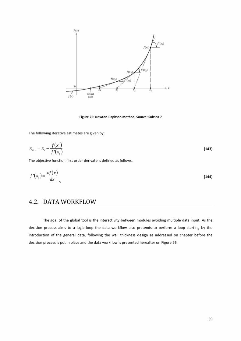
39

Figure 25: Newton-Raphson Method, Source: Subsea 7

The following iterative estimates are given by:

i

i

iixf

xfxx

'1

(143)

The objective function first order derivate is defined as follows.

ix

idx

xdfxf ' (144)

4.2. DATA WORKFLOW

The goal of the global tool is the interactivity between modules avoiding multiple data input. As the

decision process aims to a logic loop the data workflow also pretends to perform a loop starting by the

introduction of the general data, following the wall thickness design as addressed on chapter before the

decision process is put in place and the data workflow is presented hereafter on Figure 26.

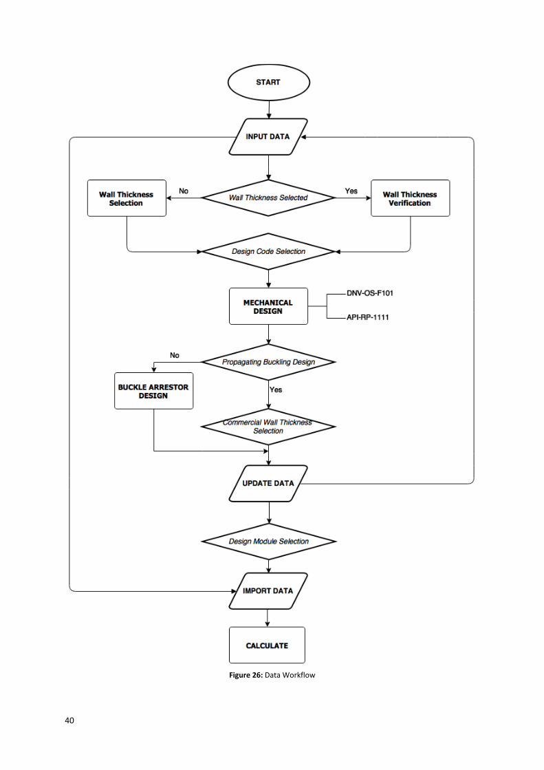
40

Figure 26: Data Workflow

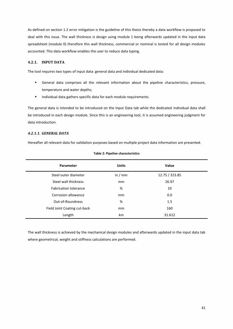
41

As defined on section 1.2 error mitigation is the guideline of this thesis thereby a data workflow is proposed to

deal with this issue. The wall thickness is design using module 1 being afterwards updated in the input data

spreadsheet (module 0) therefore this wall thickness, commercial or nominal is tested for all design modules

accounted. This data workflow enables the user to reduce data typing.

4.2.1. INPUT DATA

The tool requires two types of input data: general data and individual dedicated data:

General data comprises all the relevant information about the pipeline characteristics, pressure,

temperature and water depths;

Individual data gathers specific data for each module requirements.

The general data is intended to be introduced on the Input Data tab while the dedicated individual data shall

be introduced in each design module. Since this is an engineering tool, it is assumed engineering judgment for

data introduction.

4.2.1.1. GENERAL DATA

Hereafter all relevant data for validation purposes based on multiple project data information are presented.

Table 2: Pipeline characteristics

Parameter Units Value

Steel outer diameter in / mm 12.75 / 323.85

Steel wall thickness mm 26.97

Fabrication tolerance % 10

Corrosion allowance mm 0.0

Out-of-Roundness % 1.5

Field Joint Coating cut-back mm 160

Length km 31.612

The wall thickness is achieved by the mechanical design modules and afterwards updated in the input data tab

where geometrical, weight and stiffness calculations are performed.

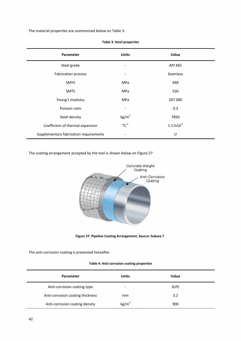
42

The material properties are summarized below on Table 3.

Table 3: Steel properties

Parameter Units Value

Steel grade - API X65

Fabrication process - Seamless

SMYS MPa 448

SMTS MPa 530

Young’s modulus MPa 207 000

Poisson ratio - 0.3

Steel density kg/m3 7850

Coefficient of thermal expansion ⁰C-1

1.17x10-5

Supplementary fabrication requirements - U

The coating arrangement accepted by the tool is shown below on Figure 27

Figure 27: Pipeline Coating Arrangement, Source: Subsea 7

The anti-corrosion coating is presented hereafter.

Table 4: Anti-corrosion coating properties

Parameter Units Value

Anti-corrosion coating type - 3LPE

Anti-corrosion coating thickness mm 3.2

Anti-corrosion coating density kg/m3 900

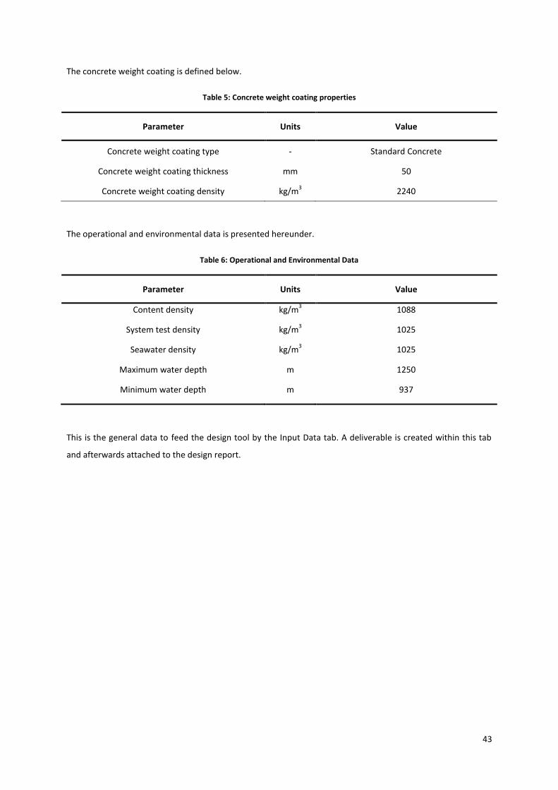
43

The concrete weight coating is defined below.

Table 5: Concrete weight coating properties

Parameter Units Value

Concrete weight coating type - Standard Concrete

Concrete weight coating thickness mm 50

Concrete weight coating density kg/m3 2240

The operational and environmental data is presented hereunder.

Table 6: Operational and Environmental Data

Parameter Units Value

Content density kg/m3 1088

System test density kg/m3 1025

Seawater density kg/m3 1025

Maximum water depth m 1250

Minimum water depth m 937

This is the general data to feed the design tool by the Input Data tab. A deliverable is created within this tab

and afterwards attached to the design report.

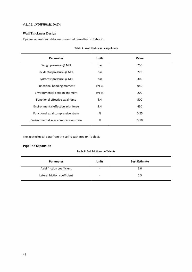
44

4.2.1.2. INDIVIDUAL DATA

Wall Thickness Design

Pipeline operational data are presented hereafter on Table 7.

Table 7: Wall thickness design loads

Parameter Units Value

Design pressure @ MSL bar 250

Incidental pressure @ MSL bar 275

Hydrotest pressure @ MSL bar 305

Functional bending moment kN·m 950

Environmental bending moment kN·m 200

Functional effective axial force kN 500

Environmental effective axial force kN 450

Functional axial compressive strain % 0.25

Environmental axial compressive strain % 0.10

The geotechnical data from the soil is gathered on Table 8.

Pipeline Expansion

Table 8: Soil friction coefficients

Parameter Units Best Estimate

Axial friction coefficient - 1.0

Lateral friction coefficient - 0.5

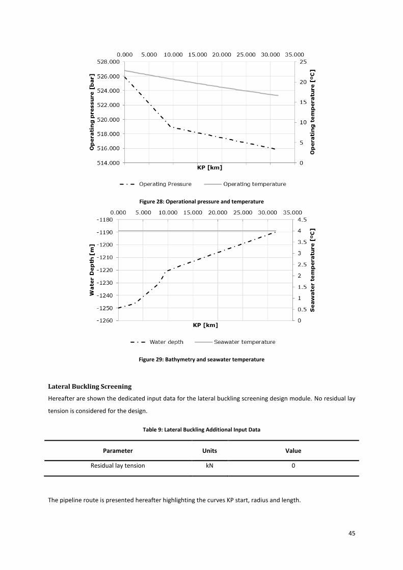
45

Figure 28: Operational pressure and temperature

Figure 29: Bathymetry and seawater temperature

Lateral Buckling Screening

Hereafter are shown the dedicated input data for the lateral buckling screening design module. No residual lay

tension is considered for the design.

Table 9: Lateral Buckling Additional Input Data

Parameter Units Value

Residual lay tension kN 0

The pipeline route is presented hereafter highlighting the curves KP start, radius and length.

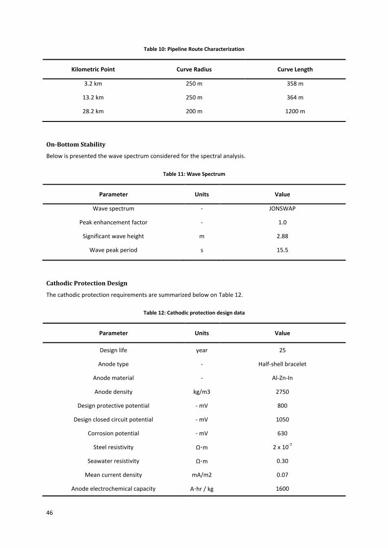
46

Table 10: Pipeline Route Characterization

Kilometric Point Curve Radius Curve Length

3.2 km 250 m 358 m

13.2 km 250 m 364 m

28.2 km 200 m 1200 m

On-Bottom Stability

Below is presented the wave spectrum considered for the spectral analysis.

Table 11: Wave Spectrum

Parameter Units Value

Wave spectrum - JONSWAP

Peak enhancement factor - 1.0

Significant wave height m 2.88

Wave peak period s 15.5

Cathodic Protection Design

The cathodic protection requirements are summarized below on Table 12.

Table 12: Cathodic protection design data

Parameter Units Value

Design life year 25

Anode type - Half-shell bracelet

Anode material - Al-Zn-In

Anode density kg/m3 2750

Design protective potential - mV 800

Design closed circuit potential - mV 1050

Corrosion potential - mV 630

Steel resistivity Ω·m 2 x 10-7

Seawater resistivity Ω·m 0.30

Mean current density mA/m2 0.07

Anode electrochemical capacity A·hr / kg 1600

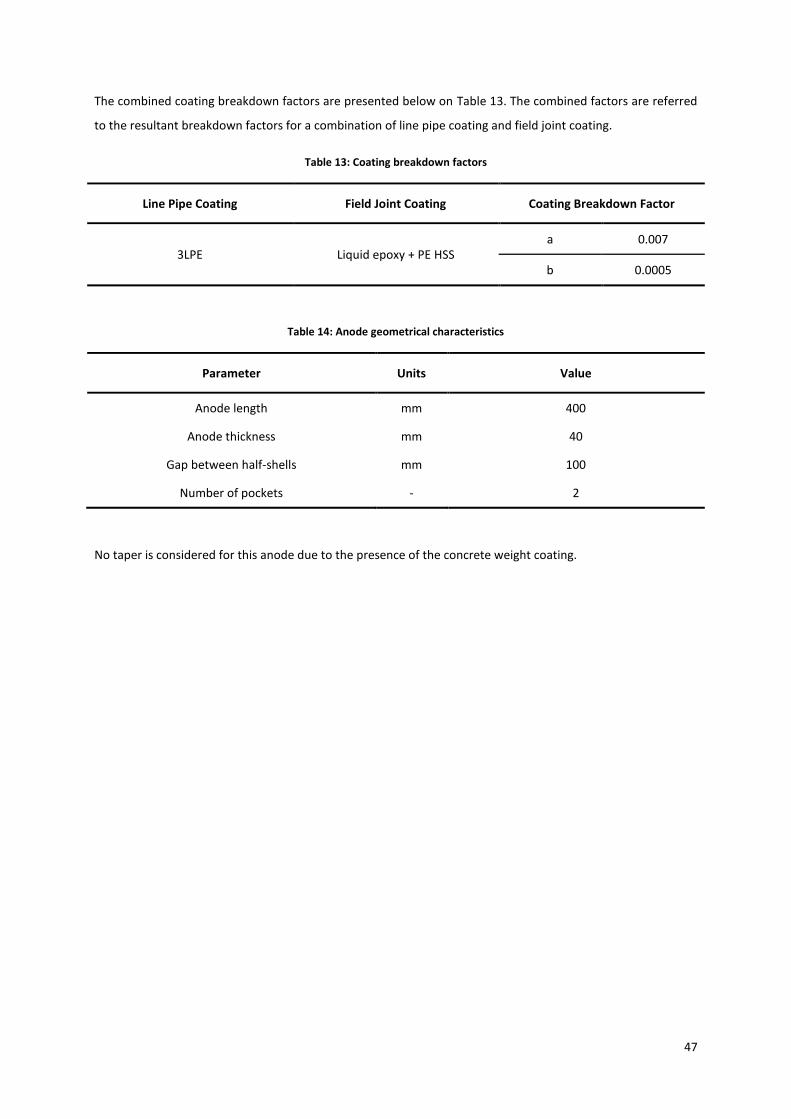
47

The combined coating breakdown factors are presented below on Table 13. The combined factors are referred

to the resultant breakdown factors for a combination of line pipe coating and field joint coating.

Table 13: Coating breakdown factors

Line Pipe Coating Field Joint Coating Coating Breakdown Factor

3LPE Liquid epoxy + PE HSS a 0.007

b 0.0005

Table 14: Anode geometrical characteristics

Parameter Units Value

Anode length mm 400

Anode thickness mm 40

Gap between half-shells mm 100

Number of pockets - 2

No taper is considered for this anode due to the presence of the concrete weight coating.

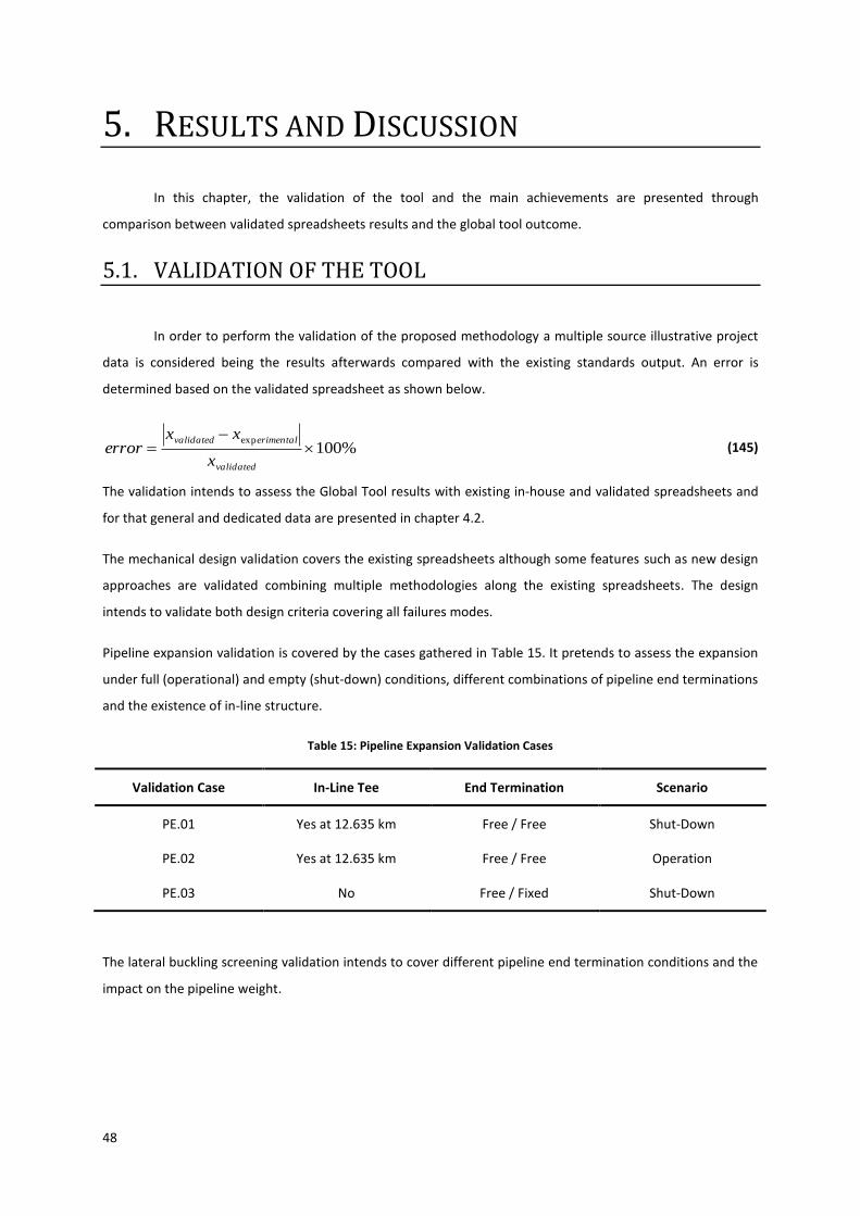
48

5. RESULTS AND DISCUSSION

In this chapter, the validation of the tool and the main achievements are presented through

comparison between validated spreadsheets results and the global tool outcome.

5.1. VALIDATION OF THE TOOL

In order to perform the validation of the proposed methodology a multiple source illustrative project

data is considered being the results afterwards compared with the existing standards output. An error is

determined based on the validated spreadsheet as shown below.

%100exp

validated

erimentalvalidated

x

xxerror (145)

The validation intends to assess the Global Tool results with existing in-house and validated spreadsheets and

for that general and dedicated data are presented in chapter 4.2.

The mechanical design validation covers the existing spreadsheets although some features such as new design

approaches are validated combining multiple methodologies along the existing spreadsheets. The design

intends to validate both design criteria covering all failures modes.

Pipeline expansion validation is covered by the cases gathered in Table 15. It pretends to assess the expansion

under full (operational) and empty (shut-down) conditions, different combinations of pipeline end terminations

and the existence of in-line structure.

Table 15: Pipeline Expansion Validation Cases

Validation Case In-Line Tee End Termination Scenario

PE.01 Yes at 12.635 km Free / Free Shut-Down

PE.02 Yes at 12.635 km Free / Free Operation

PE.03 No Free / Fixed Shut-Down

The lateral buckling screening validation intends to cover different pipeline end termination conditions and the

impact on the pipeline weight.

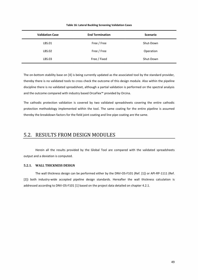
49

Table 16: Lateral Buckling Screening Validation Cases

Validation Case End Termination Scenario

LBS.01 Free / Free Shut-Down

LBS.02 Free / Free Operation

LBS.03 Free / Fixed Shut-Down

The on-bottom stability base on [4] is being currently updated as the associated tool by the standard provider,

thereby there is no validated tools to cross check the outcome of this design module. Also within the pipeline

discipline there is no validated spreadsheet, although a partial validation is performed on the spectral analysis

and the outcome compared with industry based OrcaFlex™ provided by Orcina.

The cathodic protection validation is covered by two validated spreadsheets covering the entire cathodic

protection methodology implemented within the tool. The same coating for the entire pipeline is assumed

thereby the breakdown factors for the field joint coating and line pipe coating are the same.

5.2. RESULTS FROM DESIGN MODULES

Herein all the results provided by the Global Tool are compared with the validated spreadsheets

output and a deviation is computed.

5.2.1. WALL THICKNESS DESIGN

The wall thickness design can be performed either by the DNV-OS-F101 (Ref. [1]) or API-RP-1111 (Ref.

[2]) both industry-wide accepted pipeline design standards. Hereafter the wall thickness calculation is

addressed according to DNV-OS-F101 [1] based on the project data detailed on chapter 4.2.1.

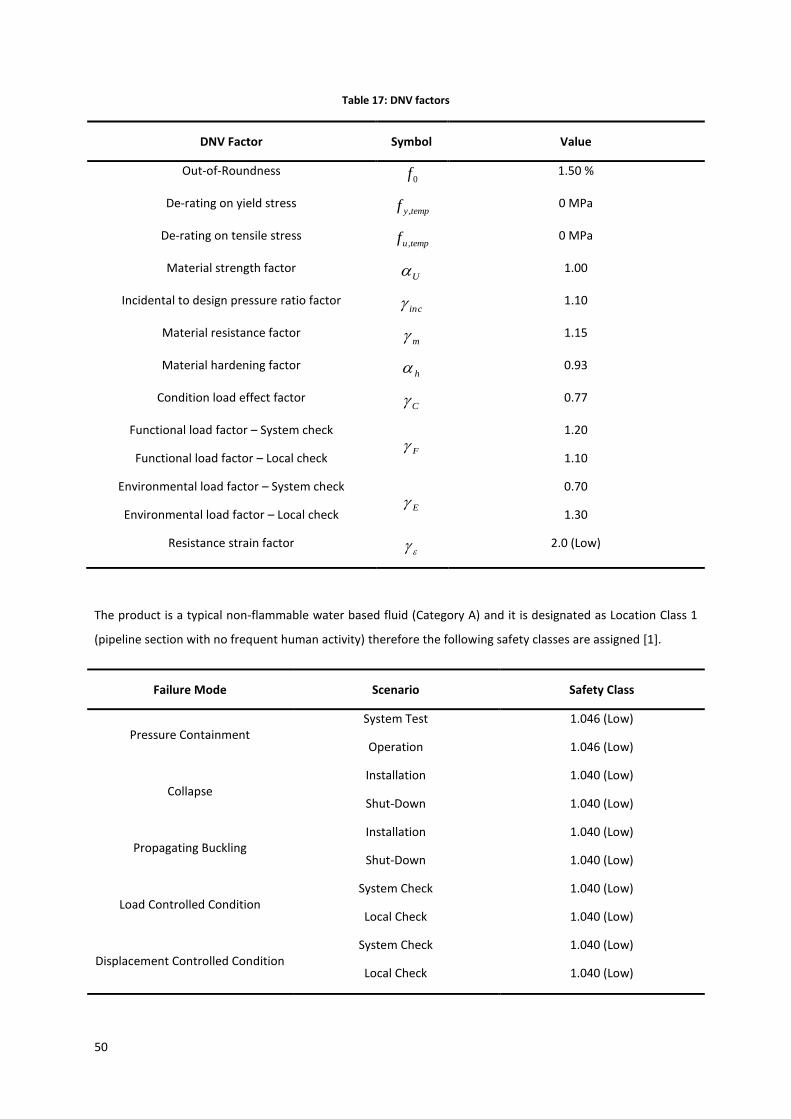
50

Table 17: DNV factors

DNV Factor Symbol Value

Out-of-Roundness 0f

1.50 %

De-rating on yield stress tempyf ,

0 MPa

De-rating on tensile stress tempuf ,

0 MPa

Material strength factor U

1.00

Incidental to design pressure ratio factor inc

1.10

Material resistance factor m

1.15

Material hardening factor h 0.93

Condition load effect factor C 0.77

Functional load factor – System check

F 1.20

Functional load factor – Local check 1.10

Environmental load factor – System check

E 0.70

Environmental load factor – Local check 1.30

Resistance strain factor 2.0 (Low)

The product is a typical non-flammable water based fluid (Category A) and it is designated as Location Class 1

(pipeline section with no frequent human activity) therefore the following safety classes are assigned [1].

Failure Mode Scenario Safety Class

Pressure Containment System Test 1.046 (Low)

Operation 1.046 (Low)

Collapse Installation 1.040 (Low)

Shut-Down 1.040 (Low)

Propagating Buckling Installation 1.040 (Low)

Shut-Down 1.040 (Low)

Load Controlled Condition System Check 1.040 (Low)

Local Check 1.040 (Low)

Displacement Controlled Condition System Check 1.040 (Low)

Local Check 1.040 (Low)

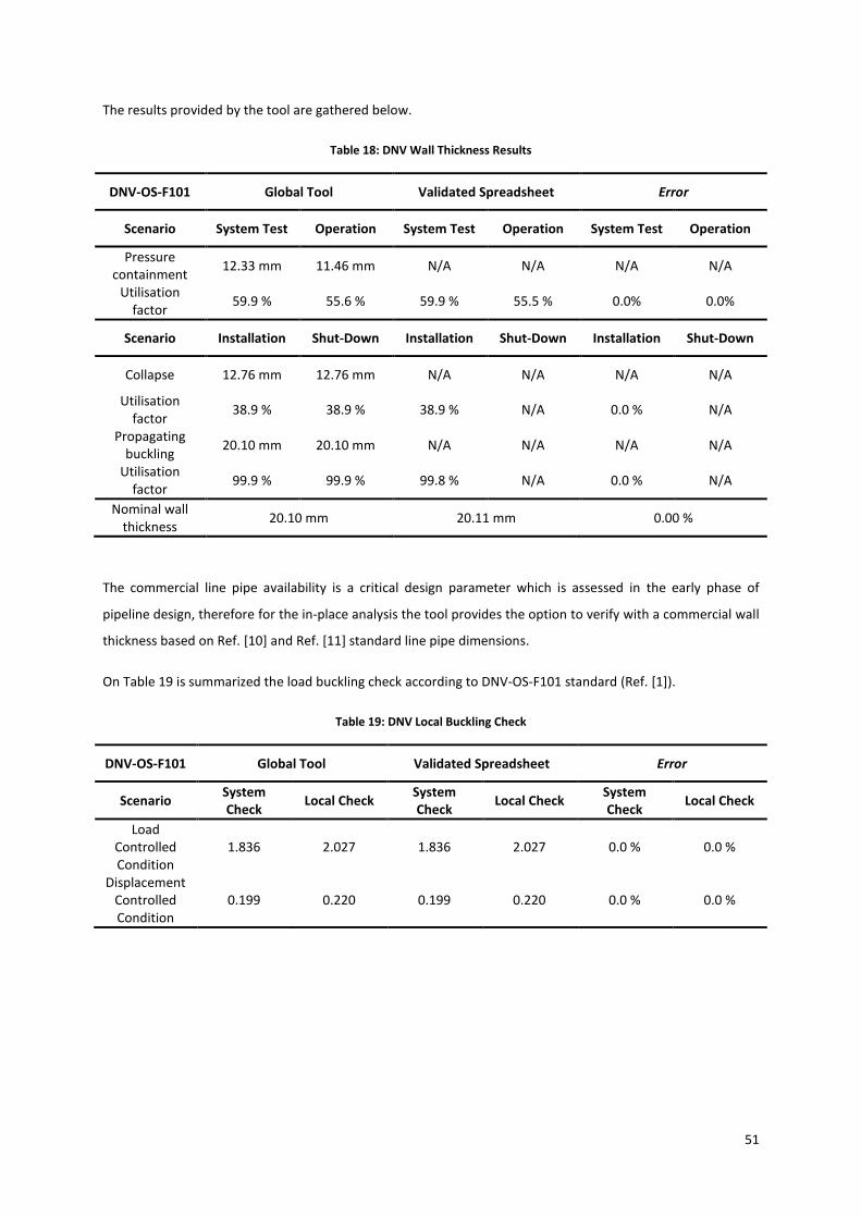
51

The results provided by the tool are gathered below.

Table 18: DNV Wall Thickness Results

DNV-OS-F101 Global Tool Validated Spreadsheet Error

Scenario System Test Operation System Test Operation System Test Operation

Pressure containment

12.33 mm 11.46 mm N/A N/A N/A N/A

Utilisation factor

59.9 % 55.6 % 59.9 % 55.5 % 0.0% 0.0%

Scenario Installation Shut-Down Installation Shut-Down Installation Shut-Down

Collapse 12.76 mm 12.76 mm N/A N/A N/A N/A

Utilisation factor

38.9 % 38.9 % 38.9 % N/A 0.0 % N/A

Propagating buckling

20.10 mm 20.10 mm N/A N/A N/A N/A

Utilisation factor

99.9 % 99.9 % 99.8 % N/A 0.0 % N/A

Nominal wall thickness

20.10 mm 20.11 mm 0.00 %

The commercial line pipe availability is a critical design parameter which is assessed in the early phase of

pipeline design, therefore for the in-place analysis the tool provides the option to verify with a commercial wall

thickness based on Ref. [10] and Ref. [11] standard line pipe dimensions.

On Table 19 is summarized the load buckling check according to DNV-OS-F101 standard (Ref. [1]).

Table 19: DNV Local Buckling Check

DNV-OS-F101 Global Tool Validated Spreadsheet Error

Scenario System Check

Local Check System Check

Local Check System Check

Local Check

Load Controlled Condition

1.836 2.027 1.836 2.027 0.0 % 0.0 %

Displacement Controlled Condition

0.199 0.220 0.199 0.220 0.0 % 0.0 %

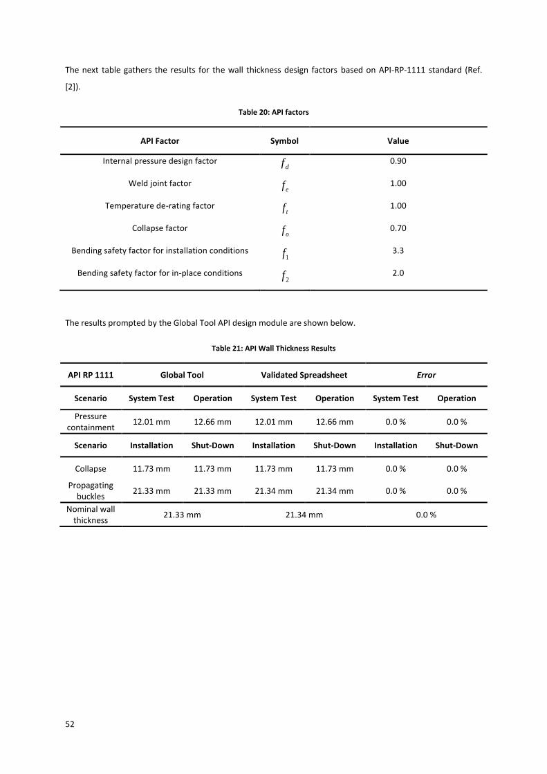
52

The next table gathers the results for the wall thickness design factors based on API-RP-1111 standard (Ref.

[2]).

Table 20: API factors

API Factor Symbol Value

Internal pressure design factor df 0.90

Weld joint factor ef 1.00

Temperature de-rating factor tf 1.00

Collapse factor of 0.70

Bending safety factor for installation conditions 1f 3.3

Bending safety factor for in-place conditions 2f 2.0

The results prompted by the Global Tool API design module are shown below.

Table 21: API Wall Thickness Results

API RP 1111 Global Tool Validated Spreadsheet Error

Scenario System Test Operation System Test Operation System Test Operation

Pressure containment

12.01 mm 12.66 mm 12.01 mm 12.66 mm 0.0 % 0.0 %

Scenario Installation Shut-Down Installation Shut-Down Installation Shut-Down

Collapse 11.73 mm 11.73 mm 11.73 mm 11.73 mm 0.0 % 0.0 %

Propagating buckles

21.33 mm 21.33 mm 21.34 mm 21.34 mm 0.0 % 0.0 %

Nominal wall thickness

21.33 mm 21.34 mm 0.0 %

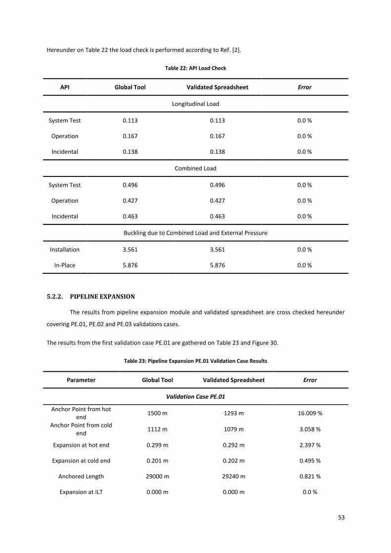
53

Hereunder on Table 22 the load check is performed according to Ref. [2].

Table 22: API Load Check

API Global Tool Validated Spreadsheet Error

Longitudinal Load

System Test 0.113 0.113 0.0 %

Operation 0.167 0.167 0.0 %

Incidental 0.138 0.138 0.0 %

Combined Load

System Test 0.496 0.496 0.0 %

Operation 0.427 0.427 0.0 %

Incidental 0.463 0.463 0.0 %

Buckling due to Combined Load and External Pressure

Installation 3.561 3.561 0.0 %

In-Place 5.876 5.876 0.0 %

5.2.2. PIPELINE EXPANSION

The results from pipeline expansion module and validated spreadsheet are cross checked hereunder

covering PE.01, PE.02 and PE.03 validations cases.

The results from the first validation case PE.01 are gathered on Table 23 and Figure 30.

Table 23: Pipeline Expansion PE.01 Validation Case Results

Parameter Global Tool Validated Spreadsheet Error

Validation Case PE.01

Anchor Point from hot end

1500 m 1293 m 16.009 %

Anchor Point from cold end

1112 m 1079 m 3.058 %

Expansion at hot end 0.299 m 0.292 m 2.397 %

Expansion at cold end 0.201 m 0.202 m 0.495 %

Anchored Length 29000 m 29240 m 0.821 %

Expansion at ILT 0.000 m 0.000 m 0.0 %

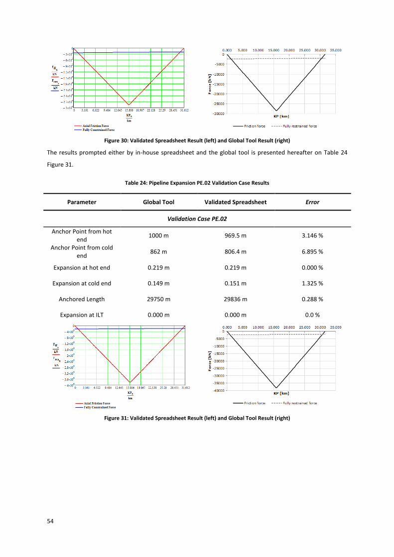
54

Figure 30: Validated Spreadsheet Result (left) and Global Tool Result (right)

The results prompted either by in-house spreadsheet and the global tool is presented hereafter on Table 24

Figure 31.

Table 24: Pipeline Expansion PE.02 Validation Case Results

Parameter Global Tool Validated Spreadsheet Error

Validation Case PE.02

Anchor Point from hot end

1000 m 969.5 m 3.146 %

Anchor Point from cold end

862 m 806.4 m 6.895 %

Expansion at hot end 0.219 m 0.219 m 0.000 %

Expansion at cold end 0.149 m 0.151 m 1.325 %

Anchored Length 29750 m 29836 m 0.288 %

Expansion at ILT 0.000 m 0.000 m 0.0 %

Figure 31: Validated Spreadsheet Result (left) and Global Tool Result (right)

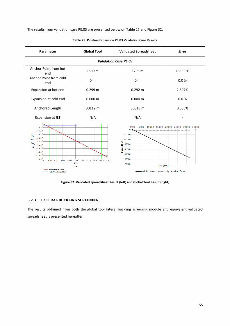
55

The results from validation case PE.03 are presented below on Table 25 and Figure 32.

Table 25: Pipeline Expansion PE.03 Validation Case Results

Parameter Global Tool Validated Spreadsheet Error

Validation Case PE.03

Anchor Point from hot end

1500 m 1293 m 16.009%

Anchor Point from cold end

0 m 0 m 0.0 %

Expansion at hot end 0.299 m 0.292 m 2.397%

Expansion at cold end 0.000 m 0.000 m 0.0 %

Anchored Length 30112 m 30319 m 0.683%

Expansion at ILT N/A N/A -

Figure 32: Validated Spreadsheet Result (left) and Global Tool Result (right)

5.2.3. LATERAL BUCKLING SCREENING

The results obtained from both the global tool lateral buckling screening module and equivalent validated

spreadsheet is presented hereafter.

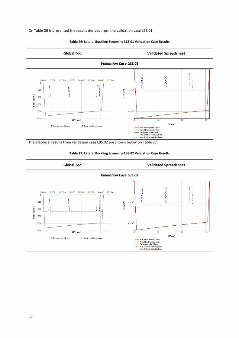
56

On Table 26 is presented the results derived from the validation case LBS.01.

Table 26: Lateral Buckling Screening LBS.01 Validation Case Results

Global Tool Validated Spreadsheet

Validation Case LBS.01

The graphical results from validation case LBS.02 are shown below on Table 27.

Table 27: Lateral Buckling Screening LBS.02 Validation Case Results

Global Tool Validated Spreadsheet

Validation Case LBS.02

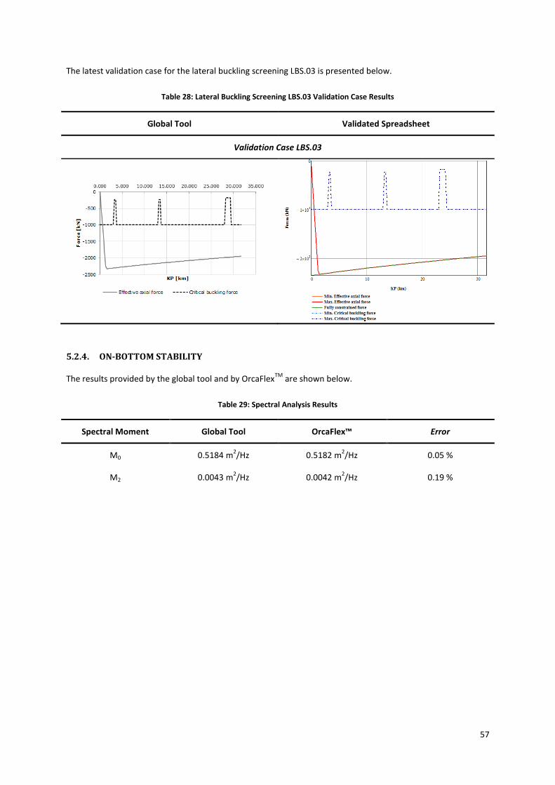
57

The latest validation case for the lateral buckling screening LBS.03 is presented below.

Table 28: Lateral Buckling Screening LBS.03 Validation Case Results

Global Tool Validated Spreadsheet

Validation Case LBS.03

5.2.4. ON-BOTTOM STABILITY

The results provided by the global tool and by OrcaFlexTM

are shown below.

Table 29: Spectral Analysis Results

Spectral Moment Global Tool OrcaFlex™ Error

M0 0.5184 m2/Hz 0.5182 m

2/Hz 0.05 %

M2 0.0043 m2/Hz 0.0042 m

2/Hz 0.19 %

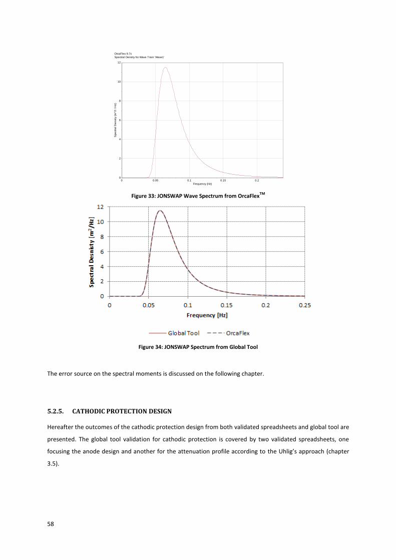
58

Figure 33: JONSWAP Wave Spectrum from OrcaFlex

TM

Figure 34: JONSWAP Spectrum from Global Tool

The error source on the spectral moments is discussed on the following chapter.

5.2.5. CATHODIC PROTECTION DESIGN

Hereafter the outcomes of the cathodic protection design from both validated spreadsheets and global tool are

presented. The global tool validation for cathodic protection is covered by two validated spreadsheets, one

focusing the anode design and another for the attenuation profile according to the Uhlig’s approach (chapter

3.5).

OrcaFlex 9.7c

Spectral Density for Wave Train 'Wave1'

Frequency (Hz)

0.20.150.10.050

Sp

ectr

al D

en

sity (

m^2

/ H

z)

12

10

8

6

4

2

0

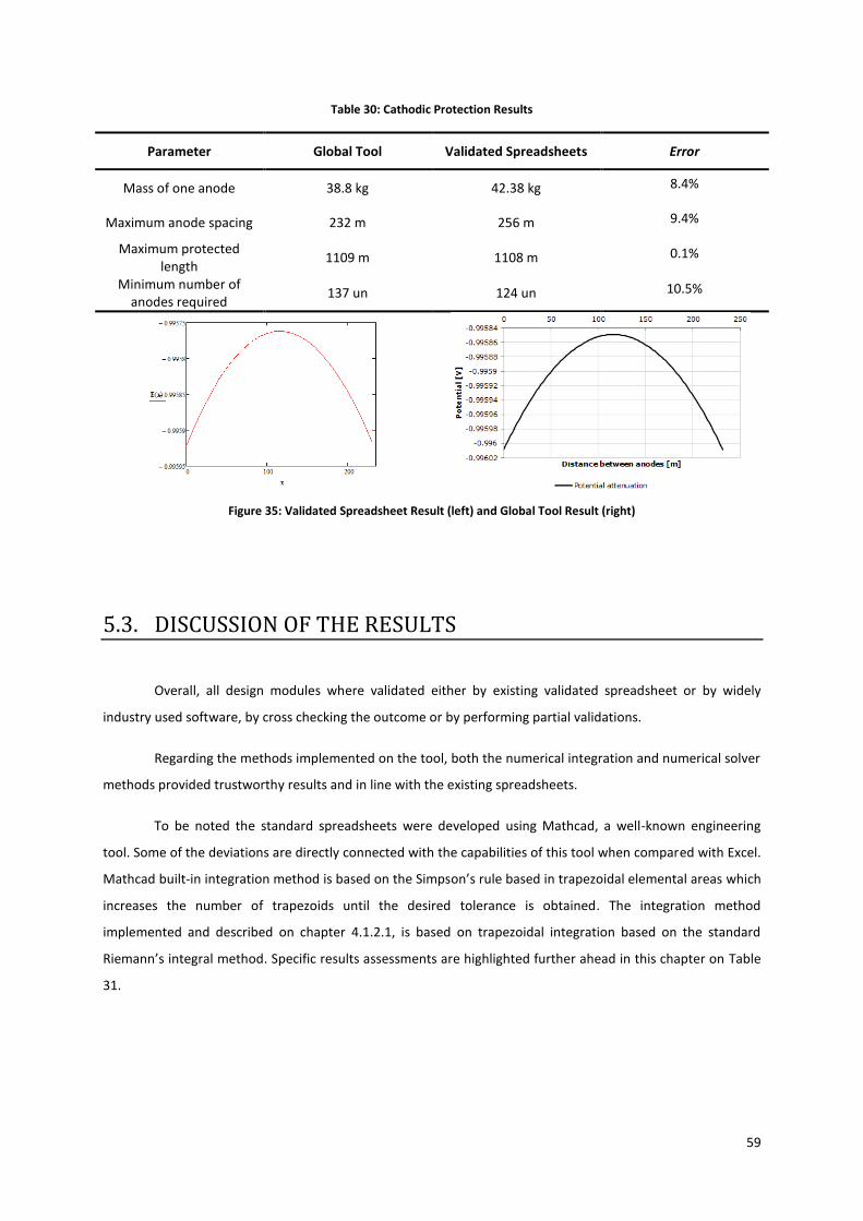
59

Table 30: Cathodic Protection Results

Parameter Global Tool Validated Spreadsheets Error

Mass of one anode 38.8 kg 42.38 kg 8.4%

Maximum anode spacing 232 m 256 m 9.4%

Maximum protected length

1109 m 1108 m 0.1%

Minimum number of anodes required

137 un 124 un 10.5%

Figure 35: Validated Spreadsheet Result (left) and Global Tool Result (right)

5.3. DISCUSSION OF THE RESULTS

Overall, all design modules where validated either by existing validated spreadsheet or by widely

industry used software, by cross checking the outcome or by performing partial validations.

Regarding the methods implemented on the tool, both the numerical integration and numerical solver

methods provided trustworthy results and in line with the existing spreadsheets.

To be noted the standard spreadsheets were developed using Mathcad, a well-known engineering

tool. Some of the deviations are directly connected with the capabilities of this tool when compared with Excel.

Mathcad built-in integration method is based on the Simpson’s rule based in trapezoidal elemental areas which

increases the number of trapezoids until the desired tolerance is obtained. The integration method

implemented and described on chapter 4.1.2.1, is based on trapezoidal integration based on the standard

Riemann’s integral method. Specific results assessments are highlighted further ahead in this chapter on Table

31.

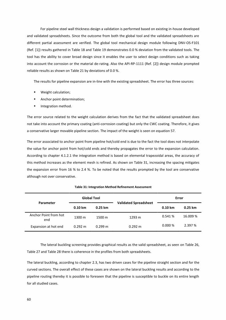
60

For pipeline steel wall thickness design a validation is performed based on existing in-house developed

and validated spreadsheets. Since the outcome from both the global tool and the validated spreadsheets are

different partial assessment are verified. The global tool mechanical design module following DNV-OS-F101

(Ref. [1]) results gathered in Table 18 and Table 19 demonstrates 0.0 % deviation from the validated tools. The

tool has the ability to cover broad design since it enables the user to select design conditions such as taking

into account the corrosion or the material de-rating. Also the API-RP-1111 (Ref. [2]) design module prompted

reliable results as shown on Table 21 by deviations of 0.0 %.

The results for pipeline expansion are in-line with the existing spreadsheet. The error has three sources:

Weight calculation;

Anchor point determination;

Integration method.

The error source related to the weight calculation derives from the fact that the validated spreadsheet does

not take into account the primary coating (anti-corrosion coating) but only the CWC coating. Therefore, it gives

a conservative larger movable pipeline section. The impact of the weight is seen on equation 57.

The error associated to anchor point from pipeline hot/cold end is due to the fact the tool does not interpolate

the value for anchor point from hot/cold ends and thereby propagates the error to the expansion calculation.

According to chapter 4.1.2.1 the integration method is based on elemental trapezoidal areas, the accuracy of

this method increases as the element mesh is refined. As shown on Table 31, increasing the spacing mitigates

the expansion error from 16 % to 2.4 %. To be noted that the results prompted by the tool are conservative

although not over conservative.

Table 31: Integration Method Refinement Assessment

Parameter

Global Tool

Validated Spreadsheet

Error

0.10 km 0.25 km 0.10 km 0.25 km

Anchor Point from hot end

1300 m 1500 m 1293 m 0.541 % 16.009 %

Expansion at hot end 0.292 m 0.299 m 0.292 m 0.000 % 2.397 %

The lateral buckling screening provides graphical results as the valid spreadsheet, as seen on Table 26,

Table 27 and Table 28 there is coherence in the profiles from both spreadsheets.

The lateral buckling, according to chapter 2.3, has two driven cases for the pipeline straight section and for the

curved sections. The overall effect of these cases are shown on the lateral buckling results and according to the

pipeline routing thereby it is possible to foreseen that the pipeline is susceptible to buckle on its entire length

for all studied cases.

61

For the on-bottom stability module the partial validation is in-line with the industry used software.

Calculations which require integration have associate errors that can be tracked until the integration method

where, as addressed before, the accuracy of the method is dependent on the element length.

The cathodic protection design module delivered trustworthy and realistic design. Deviations are

found between the tool and validated spreadsheet due to the anode sizing which therefore derives from the

anode volume calculation method. The volume calculation approach defined in the tool (equation 123) takes

into accounts several volumes, half shell gap, anti-corrosion coating and fitting tolerances. More over the tool

calculates the net anode mass which is achieved by subtracting the insert material mass (equation 126). This

error is about 9% of the required mass of one anode and propagates in the results that follow. The existing

spreadsheet over-estimates anode volumes while the global tool generates realistic volumes.

62

6. CONCLUSIONS AND FURTHER DEVELOPMENTS

The Oil&Gas service companies’ face nowadays a challenge to reduce its costs and increase its

efficiency by improving the way it works. This thesis presented a new approach to deal with the optimization

required in the pipeline discipline by delivering this engineering tool.

As specified in the objectives for this thesis a final assessment of the achievements is done below:

Development of a rigid pipeline design global tool;

Validation of the tool with existing and discipline validated standards;

Numerical iteration and integration methods delivered trustworthy results.

As said before, the global design tool is the core achievement of this thesis and enhanced the possibility to

integrate all the information, following the actual trend of Oil&Gas companies to increase efficiency. This

application enables to foresee dedicated analysis requirements in an early project stage optimizing the

engineering process.

Also the methodology applied prompted reliable results and in line with the existing standards, best practices

and lessons learned.

The extensive validation performed covered the design modules methodology and the computational approach

developed delivered expected results as any commercial software, having the capability to be improvable and

adjustable.

For conclusion the objectives proposed to develop a global rigid pipeline design tool were achieved.

Further developments for the enhancement of this thesis are proposed by introducing in the tool other

modules, such as:

Pressure calculation module focused to deliver results for the pre-commissioning team.

Other pipeline design codes such as the British Standard PD 8010-2.

Improve computational time by optimizing the VBA code and data interchangeability with Excel

interface.

63

64

7. REFERENCES

[1] DNV-OS-F101, October 2013, Submarine Pipeline Systems, Det Norske Veritas AS

[2] API-RP-1111, December 2009, Design, Construction, Operation and Maintenance of Offshore

Hydrocarbon Pipelines – Limit State Design, American Petroleum Institute

[3] SAFEBUCK JIP III, October 2014, Safe Design of Pipelines with Lateral Buckling Design Guideline

[4] DNV-RP-F109, October 2010, On-Bottom Stability Design of Submarine Pipelines, Det Norske Veritas AS

[5] DNV-RP-H103, February 2014, Modelling and Analysis of Marine Operations, Det Norske Veritas AS

[6] Ochi, M.K. and Hubble, E.N., 1976, Six Parameter Wave Spectra, Coastal Engineering, Chapter 18, p.301-

328

[7] DNV-RP-F103, October 2010, Cathodic Protection of Submarine Pipelines by Galvanic Anodes, Det

Norkse Veritas AS

[8] Uhlig, H.H. and Revie, R.W., 1985, Corrosion and Corrosion Control, 3rd edition, New York, John Wiley

and Sons, p.421-423

[9] ISO-15589-2, May 2014, Petroleum, Petrochemical and Natural Gas Industries – Cathodic Protection of

Pipeline Systems Part 2: Offshore Pipelines

[10] ASME B36.10M, August 2015, Welded and Seamless Wrought Steel Pipe, American Society of

Mechanical Engineers

[11] API 5L, July 2000, Specification for Line Pipe, American Petroleum Institute

65

66

8. APPENDIX

All the results for this dissertation are presented in this chapter.

Appendix A gathers the validation reports generated by the Global Tool.

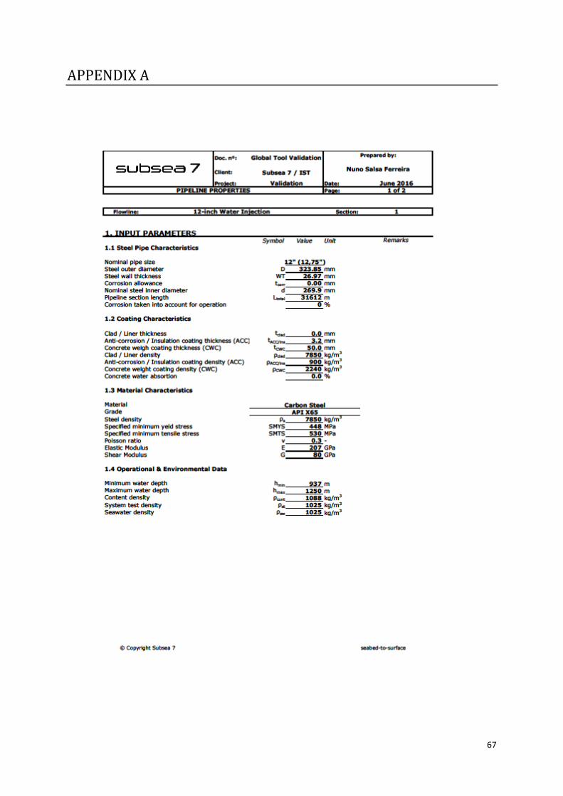
67

APPENDIX A

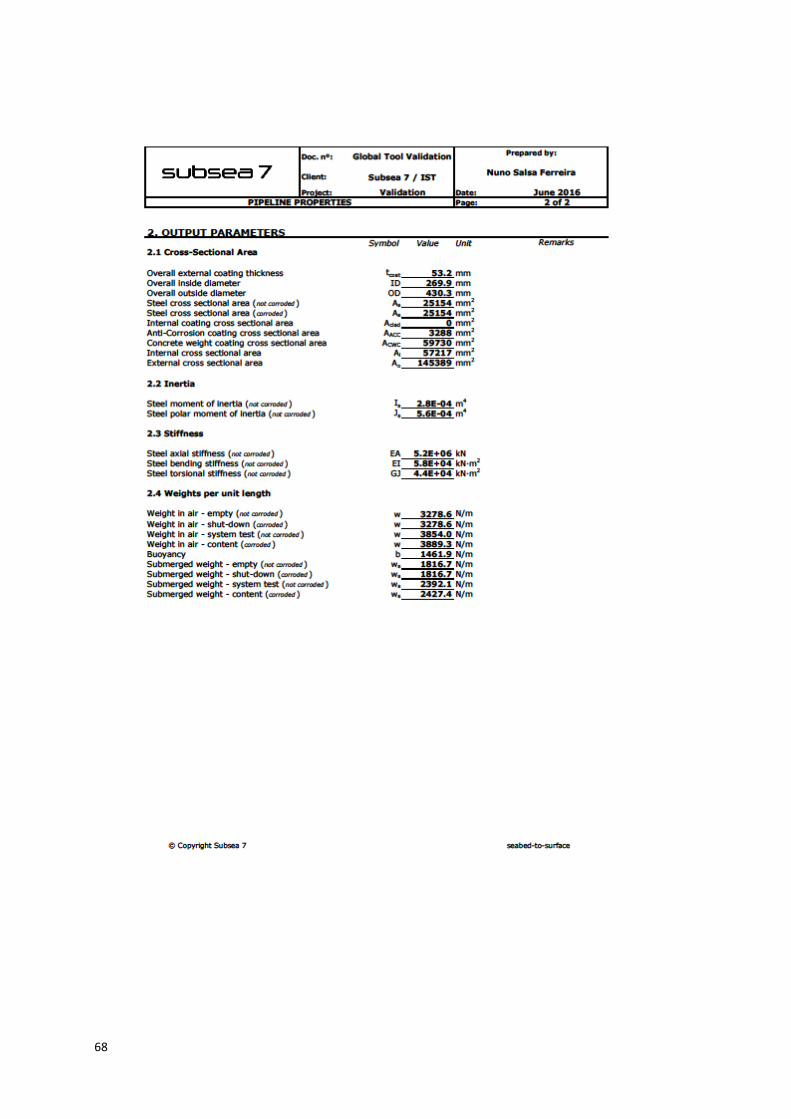
68

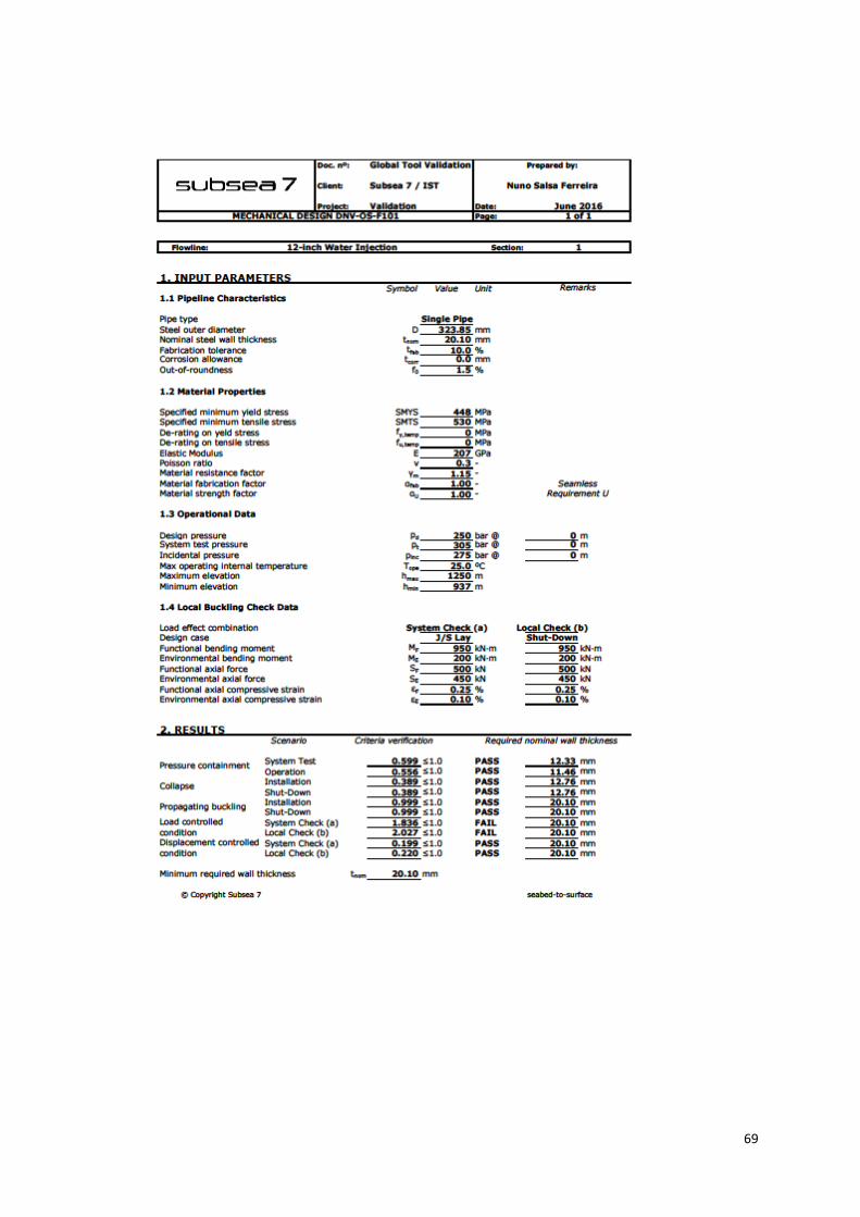
69

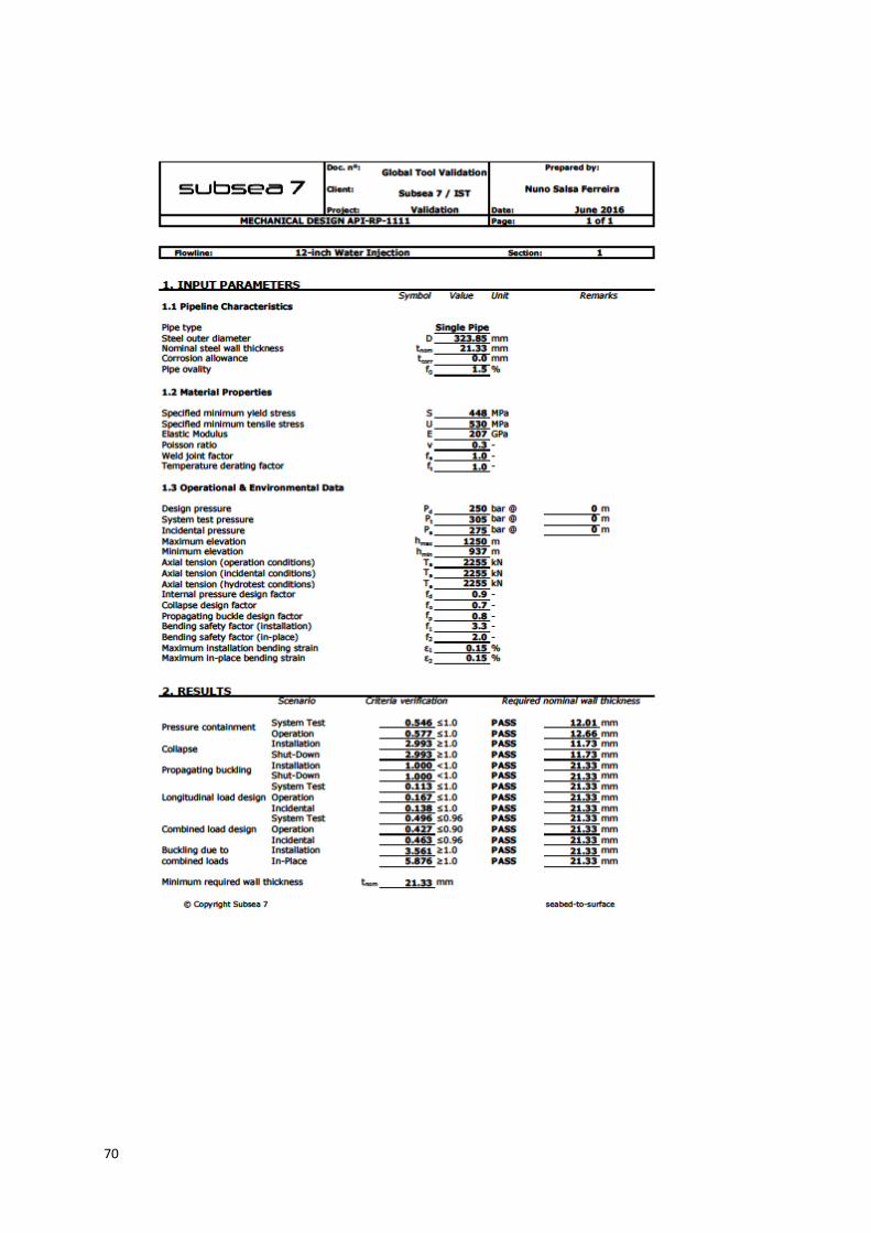
70

71

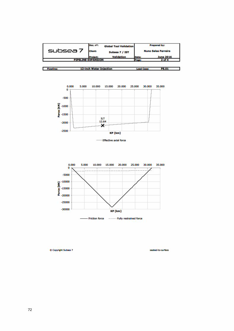
72

73

74

75

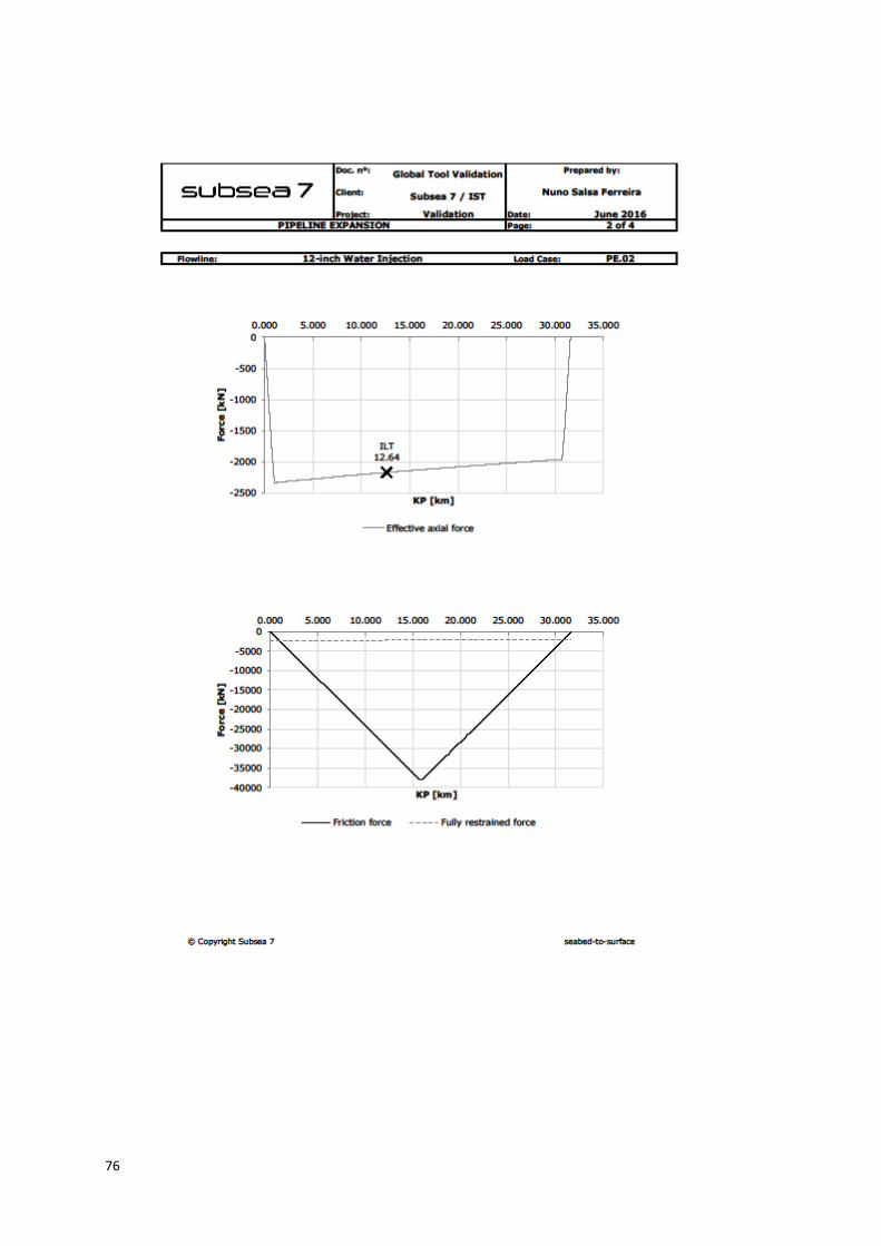
76

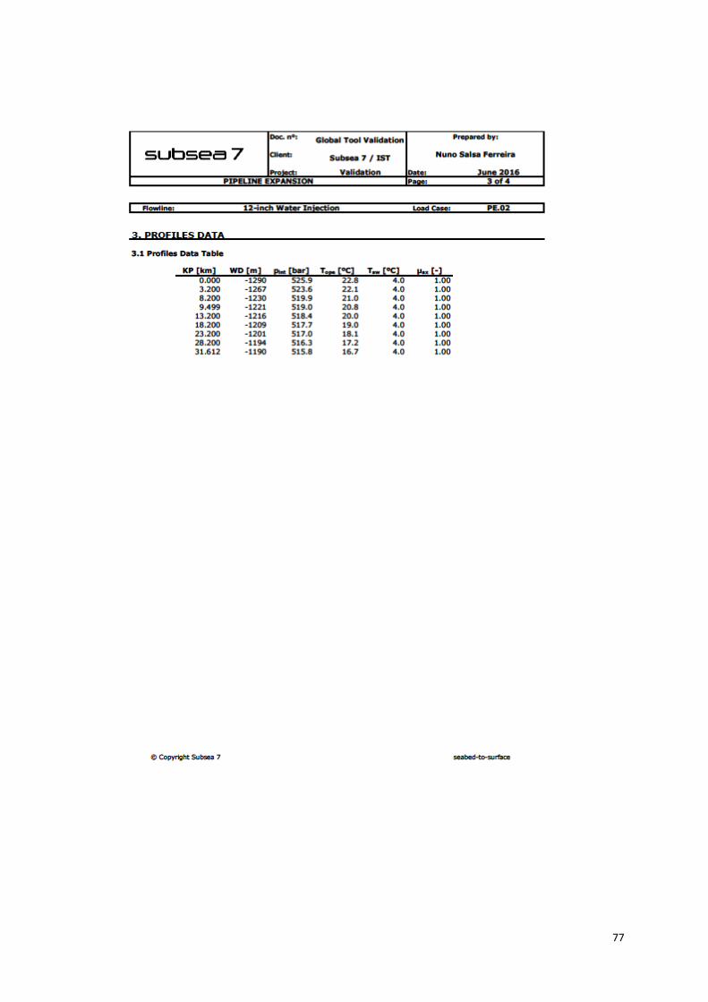
77

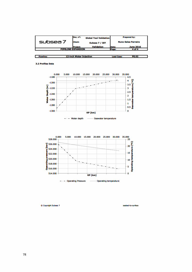
78

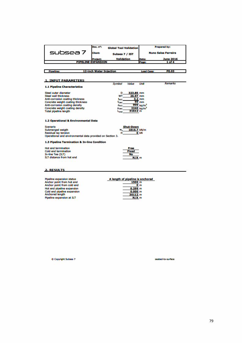
79

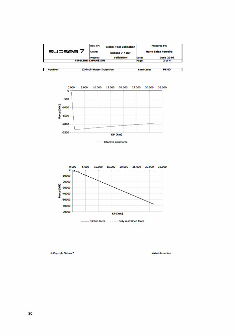
80

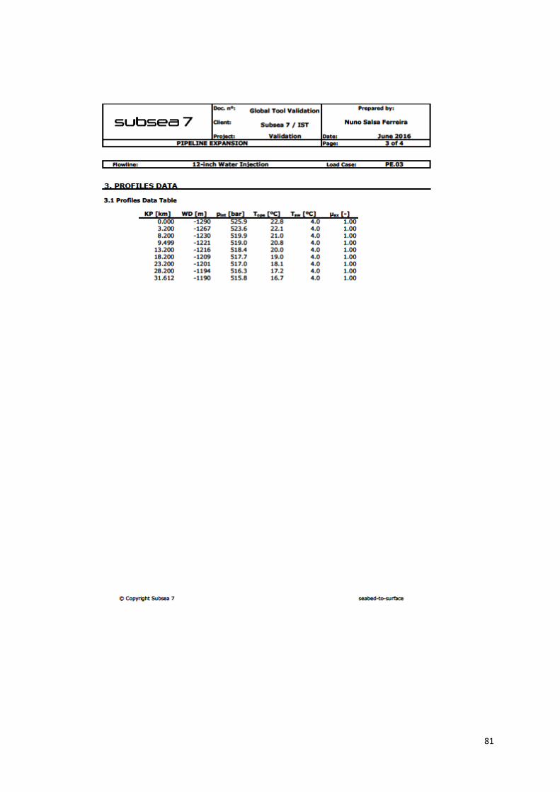
81

82

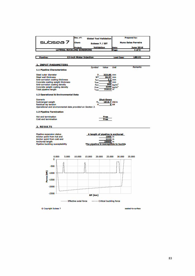
83

84

85

86

87

88

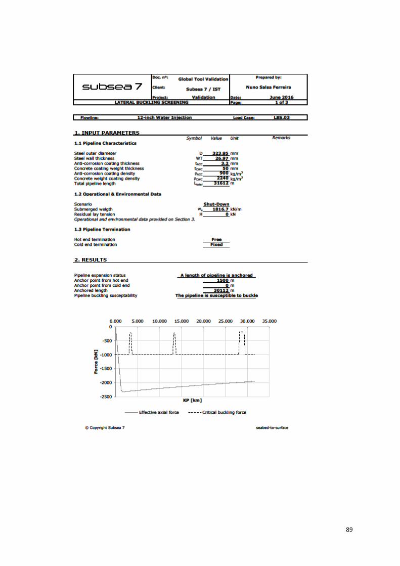
89

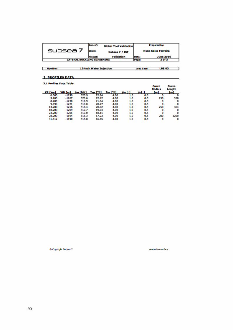
90

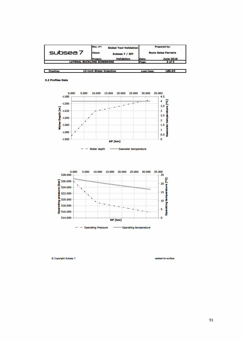
91

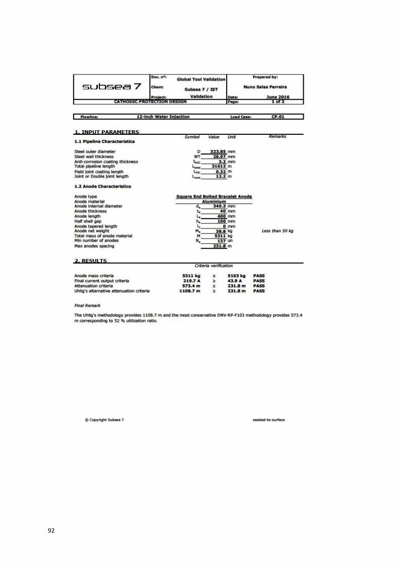
92

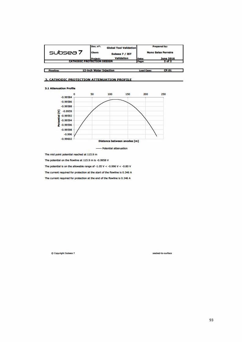
93