Species endemism: Predicting broad-scale patterns and conservation priorities

Juan Gerardo Zuloaga Villamizar

A thesis submitted to the

Faculty of Graduate and Postdoctoral Studies

in partial fulfillment of the requirements for the

Doctorate in Philosophy degree in Biology

Ottawa-Carleton Institute of Biology

Department of Biology

Faculty of Science

University of Ottawa

© Juan Gerardo Zuloaga Villamizar, Ottawa, Canada, 2018

ii

OFFICIAL STATEMENT OF WORK

Chapters in this thesis have been submitted to scientific peer-reviewed journals for publication

with the participation of my supervisor (Chapter 1 and 3) and supervisor and one co-supervisor

(Chapter 2) as co-authors. So, chapters presented here are written in first-person plural. Research

ideas, written content, analyses and figures are my own work; the co-authors provided valuable

guidance during the process. Anonymous reviewers and editors from journals (Ecography for

Chapter 1 and Global Ecology and Biogeography for Chapter 2) suggested revisions that

improved the clarity and flow of the manuscripts.

Chapter 1 has been published in the peer-reviewed journal Ecography, with the following

citation (thanks to subject editor Dr. Catherine Graham and two anonymous reviewers for their

suggestions and comments that substantially improved the final manuscript):

Zuloaga, J. and Kerr, J. T. (2017). Over the top: do thermal barriers along elevation gradients

limit biotic similarity? Ecography, 40: 478–486. doi:10.1111/ecog.01764

Chapter 2 was submitted to GEB and the editor invited submission of a revised version of

the manuscript (thanks to the subject editor Dr. Jason Pither and two anonymous reviewers for

their suggestions and comments that substantially will improve the final manuscript).

Chapter 3 will be submitted to Conservation Biology.

Finally, I would like to mention that throughout my doctorate studies I have contributed

in other research initiatives at Dr. Kerr and Dr. Currie’s labs. Some of the manuscripts ended up

in publications:

Boucher-Lalonde, V., R. De Camargo, J.M. Fortin, S. Khair S., R. So, Watson, D., Vasquez, H.,

Zuloaga, J., Currie, D (2015). The weakness of the evidence supporting tropical niche

iii

conservatism as a main driver of current richness–temperature gradients. Global Ecology

and Biogeography, 24(7):795-803.

Leroux, S., M. Larrivee, V. Boucher-Lalonde, A. Hurford, J. Zuloaga, J. T. Kerr, and F.

Lutscher. 2013. Mechanistic models for the spatial spread of species under climate

change. Ecological Applications, 23:815-828

Schick, A., J. Dench, V. Boucher-Lalonde, M. Sawatzky, A. Melnyk, J. Zuloaga, D. Currie, and

J. Kerr. In preparation. Specialization is not a mechanism by which environmental

heterogeneity determines global patterns of species richness.

Coristine, L., P. Galpern, A. Plowright, C. Robillard, E. Acheson, R. Soares, A. Pindar, J.

Zuloaga & J. Kerr. Submitted. Climate change exposure: a new technique to identify

regions with lower rates and variability of climate change at continental scales.

iv

ACKNOLEDGEMENTS

I would like to thank my supervisor Dr. Jeremy Kerr, who supported me from the beginning to

the end of my doctorate. It was a long path, with multiple disappointments and few but

rewarding successes. He was there all time, unconditionally, to encourage me to pursue my

goals. I learnt from him not only how to become a scientist, but on how to achieve excellence

and how our work in science can have immense implications in our lives and the lives of others.

Thanks for sharing with me your values and how to put them into practice.

I am grateful to my colleagues at the Kerr Lab that help me in one way or another to succeed in

this endeavour. Thanks Cassandra, Emily, Laura, Rosie, Alana, Bronwyn, Max, Shawn, Paul and

many other that make learn and laugh. I would like to thank also my college from the Currie Lab,

Dr. Hector Vasquez, for his friendship and for our endless discussions about macroecology.

Thank to Peter Soroye for editing chapter 3 and general introduction and conclusion.

I would like to thank also my committee members: Dr. David Currie and Dr. Tom Sherratt for

giving me valuable feedback on my research projects. Thanks Dr. Currie for showing me the

path to the basics in science and his philosophy of science.

Thanks to my thesis defence members for their comments and suggestions to improve this thesis:

Dr. Heather Kharouba, Dr. David Currie, Dr. Tom Sherrat and Dr. Paul Martin.

Thanks to my family for your love and support. Thanks to my lovely wife for her love and

unconditional support to embark in this journey. Thanks to my daughters and grandkids, you

inspired me to make my everyday work honest, lasting and positive. My father and my mother

for your incommensurable effort to help me grow.

v

I would like to thank the University of Ottawa for giving me the Graduate Admission

Scholarship. It really helped me to pursue my degree.

To Canada, its institutions and people for giving me and my family the opportunity to start a new

life and be an active part of this society.

vi

ABSTRACT

Do thermal barriers limit biotic composition and community similarity, potentially

helping to shape biodiversity patterns at continental scales? Are environmental variables

responsible for broad-scale patterns of species endemism? Are these patterns predictable? And,

how can patterns of endemism can inform global conservation strategies? These are some of the

questions that I attempted to answer during my doctoral research.

In the first chapter, I tested one of the most contentious hypotheses in ecology: Do

thermal barriers, which grow stronger along elevational gradients across tropical mountains,

create a dispersal barrier to organisms and consequently contribute to the isolation and

divergence of species assemblages? If so, do patterns potentially generated by this mechanism

detectably relate to dissimilarity of biotic assemblages along altitudinal gradients across the

mountains in the Americas? We found that mountain passes are not only higher in tropical

realms, as initially thought by Janzen (1967), and extensively popularized and assumed in further

research, but they are also present in temperate regions along the western coast of North

America. We also found that the stronger the thermal barrier, the higher the dissimilarity

between communities. However, the variance explained was low, suggesting thermal barriers

play a minor role in creating and maintaining patterns of biodiversity.

The second chapter raises the question of why are there more small-ranged species in

some places than in others. I tested four macroecological hypotheses (H1: climate velocity; H2:

climate seasonality; H3: climate distinctiveness or rarity; and, H4: spatial heterogeneity in

contemporary climate, topography or habitat) to predict broad-scale patterns of species

endemism, using a cross-continental validation approach. We found that there is no empirical

reason, from the standpoint of model fitting, parameter estimates, and model validation, to claim

vii

that any of these hypotheses creates and maintains broad-scale patterns of endemism. Although

we found statistically significant relationships, they failed stronger tests of a causal relationship,

namely accurate prediction. That is, the hypotheses did not survive the test of cross-continental

validation, failing to predict observed patterns of endemism. Climate velocity was dropped from

some models, suggesting that early correlations in some places probably reflect collinearity with

topography. The effect of richness on endemism was in some cases negligible, suggesting that

patterns of endemism are not driven by the same variables as total richness. Despite low

explained variance, spatial heterogeneity in potential evapotranspiration was the most consistent

predictor in all models.

The third chapter is aimed to evaluate the extent to which global protected areas (PAs) have

included endemic species (species with small range size relative to the median range size). We

measure the relative coverage of endemic species by overlapping species geographic ranges for

amphibians, mammals, and birds, with the world database of PAs (1990-2016). Then we measure

the rate of expansion of the global PA network and the rate of change in endemic species coverage.

We found that ~30% of amphibian, ~6% of bird and ~10% of mammal endemic species

are completely outside PAs. Most endemic species’ ranges intersect the PA network (amphibian

species = 58%; birds = 83%; mammals = 86%), but it usually covers less than 50% of their

geographic range. Almost 50% of species outside the PA network are considered threatened

(critically endangered, endangered and vulnerable). We identified that ecoregions in tropical

Andes, Mesoamerica, Pacific Islands (e.g., New Guinea, Solomon), Dry Chaco, and Atlantic

forests are major conservation priorities areas.

The historic rates of new PAs added every year to the network is between ~6,000 to

~15,000. In contrast, we found that rates of including endemic species within the PA network have

viii

been fairly slow. Historic data shows that every year, the entire geographic range of 3 (amphibians)

to 6 (birds and mammals) endemic species is 100% included inside the PA network (amphibians

= from 162 to 233; mammals = 10 to 84; and, amphibians = 16 to 99). Based on these trends, it is

very unlikely PAs will include all endemic species (14% total endemic species, that is ~1,508 out

of 11,274) currently outside the PA network by 2020. It will require five times the effort made in

the last two decades. However, projections also showed that is very likely that some portions of

the geographic ranges for all endemic birds and mammals, but not for all endemic amphibians,

will be covered by the future PA network.

I sum, I found that none of the hypotheses tested here can explain broad-scale patterns of

total species richness and total species endemism. My main contribution on this research area is

clearly rejecting these hypotheses from potential candidates that may explain biodiversity

patterns. By removing them, we advance in this field and open possibilities to test new

hypotheses and evaluate their mechanisms. I proposed that other drivers and mechanisms

(whether biotic and biotic) acting at local scales, and escaping the detection of macroecological

approaches, might be responsible for these patterns. Finally, in terms of conservation planning, I

proposed that the international community has an opportunity to protect a great number of

endemic species and their habitats before 2020, if they strategically create new PAs.

ix

TABLE OF CONTENTS

OFFICIAL STATEMENT OF WORK ......................................................................................................... ii

ACKNOLEDGEMENTS ............................................................................................................................. iv

ABSTRACT ................................................................................................................................................. vi

TABLE OF CONTENTS ............................................................................................................................. ix

LIST OF TABLES ....................................................................................................................................... xi

LIST OF FIGURES .................................................................................................................................... xiv

GENERAL INTRODUCTION ................................................................................................................. xxiii

CHAPTER 1. Over the top: do thermal barriers along elevation gradients limit biotic similarity? ............. 1

ABSTRACT .............................................................................................................................................. 1

INTRODUCTION .................................................................................................................................... 2

MATERIAL AND METHODS ................................................................................................................ 4

Topography and thermal barriers ......................................................................................................... 4

Assemblage similarity ........................................................................................................................... 6

Thermal barriers separating assemblages ............................................................................................ 8

Statistical Analysis ................................................................................................................................ 8

RESULTS ................................................................................................................................................. 9

DISCUSSION ......................................................................................................................................... 11

ACKNOWLEDGEMENTS .................................................................................................................... 15

TABLES ................................................................................................................................................. 16

FIGURES ................................................................................................................................................ 17

CHAPTER 2. The origins and maintenance of global species endemism .................................................. 22

ABSTRACT ............................................................................................................................................ 22

INTRODUCTION .................................................................................................................................. 24

MATERIAL AND METHODS .............................................................................................................. 27

Species distributions ........................................................................................................................... 27

Spatial resolution ................................................................................................................................ 27

Measuring species endemism .............................................................................................................. 27

Spatial taxonomic congruence of patterns of endemism ..................................................................... 28

x

Climate and geographical predictors ................................................................................................... 29

Statistical analysis ............................................................................................................................... 31

RESULTS ............................................................................................................................................... 34

Spatial distribution of broad scale patterns of endemism ................................................................... 34

Metrics of endemism ........................................................................................................................... 34

Endemism and predictors relationships .............................................................................................. 35

DISCUSSION ......................................................................................................................................... 37

ACKNOLEWGMENTS ......................................................................................................................... 43

TABLES ................................................................................................................................................. 44

FIGURES ................................................................................................................................................ 48

CHAPTER 3. Endemic species coverage by the global protected areas network ...................................... 53

ABSTRACT ............................................................................................................................................ 53

INTRODUCTION .................................................................................................................................. 54

METHODS ............................................................................................................................................. 56

RESULTS ............................................................................................................................................... 58

DISCUSSION ......................................................................................................................................... 61

ACKNOWLEDGEMENTS .................................................................................................................... 66

TABLES ................................................................................................................................................. 67

FIGURES ................................................................................................................................................ 69

GENERAL CONCLUSION ....................................................................................................................... 83

REFERENCES ........................................................................................................................................... 87

APPENDICES CHAPTER 1 .................................................................................................................... 116

APPENDICES CHAPTER 2 .................................................................................................................... 124

xi

LIST OF TABLES

Table 1.1. Compositional similarity (COMP) as a function of tha maximum thermal overlap

(TOV) and accounting for geographical distance (DIST) for pairwise comparison of

quadrats in the highlands (a, b) and lowlands (c, d) in the Americas. .............................. 16

Table 2.1. Spearman’s rank correlation coefficients among metrics of endemism for a)

amphibians and b) mammals; and, c) between total species richness and five metrics of

endemism. Metrics of endemism were constructed using range size cut-offs (first quartile,

50K km2 and 250K km2), inverse range size (Weighted endemism, WE) and median

range size (Median). Note that the negative correlations involving Median are to be

expected: larger median range size implies fewer range-restricted species. .................... 44

Table 2.2. Estimates from the relationship between endemism for a) amphibians and b) mammals

and various predictors. We presented results for two metrics of endemism that we could

transform: Median range size = Sqrt(Median) and Weighted endemism = Log10(WE). For

predictors, we used: CV = Log10(Climate velocity); MATS = Seasonality in mean annual

temperature; CD_PT = Climate distinctiveness (rarity) in total precipitation; and,

SH_PET = Log10(Spatial heterogeneity in potential evapotranspiration)......................... 45

Table 2.3. Model selection for amphibians (a, b) and mammals’ (c, d) endemism (Weighted

endemism = WE (a, c); and Median range size (b, d)) as a function of various predictors:

CV = Log10(Climate velocity for); MATS = seasonality in mean annual temperature;

CD_PT = Climate distinctiveness (rarity) in total precipitation; SH_PET = Log10(Spatial

heterogeneity in potential evapotranspiration); and, Richness = Total species richness. In

bold best model. ................................................................................................................ 47

xii

Table 3.1. Number of endemic species that overlap (inside or intersect) or not (outside) with

Protected Areas (PAs). Values in parenthesis represent the proportion (%) of species in

each category within that taxon. Endemic species are based on median range size.

“Inside” indicates that polygons of species’ ranges are 95% or more contained within the

PA network; “outside” indicates species ranges totally outside the PA network;

“intersect” indicates overlap of species geographic ranges with the PA network in three

categories: between 75% - 95%, 50% - 75% and less than 50%. ..................................... 67

Table 3.2. Top 20 countries harboring the highest number of endemic species outside the

protected terrestrial areas (PAs) network for amphibians, birds and mammals. Countries

holding high numbers of endemic species for: three taxonomic groups (red), two taxa

(blue), and one taxon (black). ........................................................................................... 68

Appendices

Table S1.1. Models for thermal overlap (y) as a function of elevation (x) in the Americas.

Coordinates indicate the focal site at 300 masl used to compare measurements of thermal

regimes with all sites encounter towards the highest elevation in the mountaintop. ...... 116

Table S2.1. Non-parametric correlations coefficients (Spearman rank, rs) between endemism for

mammals and amphibians and environmental predictors. Metrics of endemism based on

species range size cut-offs (QE = first quartile; 50K = 50,000 km2 and 250K = 250,000

xiii

km2), inverse range size (WE = Weighted Endemism) and median range size (Median).

Results shown are for c. 110 km x 110 km spatial resolution. ....................................... 124

Table S2.2. Spearman correlation coefficients (r) between amphibians’ endemism and several

predictors at different spatial resolutions. We used four metrics to calculate endemism

based on range size (QE= first quartile; 50K=50,000 km2 and 250K=250,000 km2),

inverse range size (WE = Weighted Endemism), and median range size. ..................... 126

Table S2.3. Spearman correlation coefficients (r) between mammals’ endemism and several

predictors at different spatial resolutions. We used five metrics to calculate endemism

based on range size (QE= first quartile; 50K=50,000 km2 and 250K=250,000 km2),

inverse range size (WE = Weighted Endemism) and median range size (Median)........ 131

Table S2.4. Poisson, Hurdle and Zero-Inflated Poisson (ZIP) models form amphibians and

mammals’ endemism. ..................................................................................................... 137

xiv

LIST OF FIGURES

Figure 1.1. Conceptual diagram showing Janzen’s approach (Janzen, 1967), as adapted to

measure the overlap between thermal regimes of 404 focal sites (a ~1 km2 pixel) relative

to all other sites in the Americas (a). These were divided into two sets of 101 focal site

pairs at identical latitudes and elevations: the first set of 101 focal site pairs is at high

elevation (2000 metres above sea level), and the second set is at low elevation (300

metres above sea level). The sites in each pair are separated by the dividing mountain

ranges of the western Americas (b). We placed ~100 km2 quadrats over each of focal

sites to assess that area’s assemblage of mammals and amphibians. Minimum and

maximum monthly temperatures were extracted, pixel by pixel, throughout the Americas

(c). We used these values to quantify thermal overlap between each focal site and all

others using Janzen’s equation (d). R1i is the seasonal thermal regime of a focal site, R2i is

the thermal regime for a compared site, and di is the overlap between them. This resulted

in 404 thermal overlap maps of the Americas, relative to each focal site (e). Thermal

overlap ranges from pale yellow, which represents complete overlap between two thermal

regimes for every month (a value of 12) to purple, which represents maximum observed

separation between thermal regimes (i.e., areas with negative values indicates a

substantial thermal regime difference with respect to this example focal site). A thermal

barrier between two sites is the maximum difference in thermal overlap encountered

between them (f). .............................................................................................................. 17

Figure 1.2. Changing thermal overlap relative to latitude along elevational gradients in the

mountain ranges of the Americas. Black dots (left panel) represent slopes of thermal

overlap relative to elevation measured from east of the dividing mountain ranges to the

xv

peak elevation within them, while magenta triangles represent same trend measured from

the west. The gray region indicates an area where thermal overlap is not linearly related

to elevation and linear regression slope values are consequently not shown. Two panels

on the right give detailed examples showing how thermal overlap changes apparently

linearly from low with elevation in many areas. The middle panel on the right shows a

shallow thermal overlap slope (s= - 2.97 X 10-3) for temperate zones and the third panel

shows the steepest thermal overlap slope (s= -7.23 X 10-3) for tropical regions. ............. 19

Figure 1.3. Maximum difference in thermal overlap between two sites across dividing mountain

ranges in the Americas. Focal sites being compared along an elevational gradient are (a)

low to high elevation focal sites on the western slopes of mountain ranges shown in

Figure 1.1a, (b) low to high elevation focal sites along the eastern slopes of those

mountain ranges, (c) focal sites between high elevations and (d) focal sites between low

elevations. For instance, (a) shows the maximum difference in thermal overlap

encountered between a low elevation focal site at 300 m (W) and a nearby high elevation

focal site at 2000 m (w). This difference in thermal overlap represents the thermal barrier

that an organism must overcome when dispersing between focal sites. Scatterplots with

Loess curves are shown. Dashed lines show the point at which thermal overlap declines

to zero................................................................................................................................ 20

Figure 1.4. Relationships between assemblage similarity for amphibians and mammals as a

function of the maximum thermal overlap (controlling for pairwise geographic distances)

between quadrats located at (a) high elevations (2000 m) and (b) low elevations (300 m).

Red triangles represent tropical pairwise comparisons and blue dots represent temperate

ones. Letters in the top right of each graph indicate the focal site from which the thermal

xvi

overlap was measured (note that quadrats are centered on each focal site). For instance, in

the first graph, we indicates focal sites located at 2000 m, one set in the west (w) and the

other set in the east (e). The first letter indicates which focal site was used to initiate

thermal overlap measurements. For instance, we uses the thermal overlap value

calculated from a focal site located to the west (w, at 2000 m), whereas in the second

graph (ew), the thermal overlap value used is from a focal site located to the east of the

dividing range (e, at 2000 m). Stronger thermal barriers between sites are suggested by

negative thermal overlap values. ....................................................................................... 21

Figure 2.1. Broad-scale patterns of endemism (a) spatial distribution of mammals and

amphibians’ endemism, and (b) areas of taxonomic congruence within major centers of

endemism (i.e., overlapping areas of endemics species for mammals and amphibians at

100 km x 100 km spatial resolution). Taxonomic congruence was measured as follows:

for metrics based on range size cut-offs (smallest quartile, 50,000 km2, 250,000 km2) we

used four bins for proportion of endemics (0-25%, 25-50%, 50-75% and 75-100%). For

metrics based on inverse range size (weighted endemism, WE) and median range size

(Median), we calculated the difference between amphibians and mammals’ endemism

values. ............................................................................................................................... 48

Figure 2.2. Observed vs predicted values of broad-scale patterns of total species endemism

(Log10) for a) amphibians and b) mammals using a cross-continental approach (i.e.,

models used the data from all zoogeographic realms from Holt et al. (2013) except one to

then predict endemism on the hold-out continent). We tested four hypotheses (predictors):

H1: Climate stability (Climate velocity); H2: Climate seasonality (Seasonality in mean

xvii

annual temperature); H3: Climate distinctiveness (in total precipitation, CD_PT); and,

H4: Spatial heterogeneity (in potential evapotranspiration SH_PET)). We tested two

metrics of endemism: median range size and weighted endemism. Results are shown for

SAR models. ..................................................................................................................... 49

Figure 2.3. Best models predicting broad scale patterns of Endemism (using Median range size

as a metric of endemism) for amphibians (graphs on the left) and mammals (graphs on

the right). a) variance partitioning, b) path analysis and c) Cross-continental validation for

best models. MATS = Seasonality in mean annual temperature; SH_PET = Spatial

heterogeneity in potential evapotranspiration; AET = Actual evapotranspiration; and,

Richness = Total species richness. .................................................................................... 51

Figure 2.4. Best models predicting broad scale patterns of endemism, using log(Weighted

Endemism) as a metric of endemism for amphibians (graphs on the left) and mammals

(graphs on the right). a) variance partitioning, b) path analysis and c) Cross-continental

validation for best models. Seasonality = Seasonality in mean annual temperature;

SH_PET = Spatial heterogeneity in potential evapotranspiration; AET = Actual

evapotranspiration; and, Richness = Total species richness. ............................................ 52

Figure 3.1. Number of protected terrestrial areas (PAs) included in the global network since 1990

(thick black line), and projections to include all endemic species currently outside the PA

network (n = 1,580, black thin line) by 2020. Two additional projections are calculated

using two rates of change of endemic species coverage: low rate, purple dashed line; and

high rate, green dashed line. Projected trends of PA coverage by 2020, using minimum

(grey dashed line) and maximum (thin black line) historical rates. .................................. 69

xviii

Figure 3.2. Number of endemic species that are inside (blue line) or intersect (red line) protected

terrestrial areas (PAs) for a) amphibians, b) birds and c) mammals. Historic trend

represented by thick lines. Two projections aimed to include endemic species within the

PA network: using total number of endemic species outside current (2016) PA network

(thin line) and using the historic rate of change for species coverage (dotted line). ........ 70

Figure 3.3. Extent of protected terrestrial (PAs) areas (yellow) and geographic range size extent

endemic species outside the PA network for amphibians (green), birds (red) and

mammals (blue). ............................................................................................................... 71

Figure 3.4. Coverage of endemic species by protected terrestrial areas (PAs, data 1990-2016). a)

Total endemic species; b) Threatened endemic species (aggregated IUCN categories:

Critically endangered, Endangered and Vulnerable) from total; and, c) Extinct species.

Species geographic ranges that intersect any PA (categories in blues hues) where

subdivided according to their percentage of overlap with PAs’ extent (i.e., 75% - 95%,

50% - 75% and less than 50% of overlap). Notice that species that overlapped more than

95% with any PAs where considered inside PAs. ............................................................ 74

Figure 3.5. Number of endemic species outside Protected Areas (PAs) per country for a)

amphibians, b) birds and c) mammals. ............................................................................. 75

Figure 3.6. Ecoregions and number of endemic species completely outside protected terrestrial

areas for a) amphibians, b) birds and c) mammals. Bars represent a sample of ecoregions

with highest number of endemic species. ......................................................................... 78

Figure 3.7. Proportion of the class predicted to occur within a given cell within the extent of the

species geographic range (i.e., inside, outside or intersect the protected area network,

PAs); for a) amphibians, b) birds, and c) mammals. ........................................................ 82

xix

Appendices

Figure S1.1a. Thermal Overlap (TOV) between focal sites and their surrounding environmental

space in the eastern side of the Americas. Figure shows a selected group of sites in the (a)

highlands (b) lowlands. ................................................................................................... 118

Figure S1.2. Thermal overlap as a function of altitude: (a) This relationship is linear for most of

the Americas (three sites in eastern side), but is non-linear in some regions east of the

Rockies in North America between 33°N and 48°N (b). ................................................ 120

Figure S1.3. Elevation at which thermal overlap decreases to zero at all locations across the

Americas. ........................................................................................................................ 121

Figure S1.4. Compositional similarity between pairwise comparisons of quadrats across a

latitudinal gradient in the Americas’ mountains. (a) Amphibians and (b) Mammals.

Upper panel shows pairwise comparisons of sites between sites in the highlands and

lower panel in lowlands .................................................................................................. 122

Figure S1.5. Potential ‘passes’ in northern South America that could allow species to circumvent

thermal barriers imposed by differences in thermal regimes between focal sites. Arrows

represent potential dispersal routes. ................................................................................ 123

Figure S2.1. Broad scale patterns of amphibian endemism using five metrics and four spatial

resolutions. Metrics were constructed using range size cut-offs (first quartile, 50K km2

and 250K km2 ), inverse range size (Weighted Endemism, WE) and median range size.

......................................................................................................................................... 138

xx

Figure S2.2. Broad scale patterns of mammal endemism using five metrics and four spatial

resolutions. Metrics were constructed using range size cut-offs (first quartile, 50K km2

and 250K km2) and inverse range size (Weighted Endemism, WE), and median range

size. ................................................................................................................................. 139

Figure S2.3. Spatial congruence between mammals and amphibians using various metrics of

endemism a) Inverse range size, b) Median range size, c) Range size threshold (smallest

quartile), and d) Range size threshold (<50,000 Km2). .................................................. 140

Figure S2.4a. Number of endemic species (boxplots) in mountain systems (300 to 2,500 meters

above the sea level) along a latitudinal gradient (greyscale bands represent approximately

10 degrees) for a) amphibians and b) mammals. ............................................................ 141

Figure S2.5. Proportion of species with small range size within areas of high species richness

(highest quantile) for amphibians (left graphs) and mammals (right graphs), using the

highest quartile of two metrics of species endemism a) range size cut-off = Quantile and

b) range size cut-off = 50,000 Km2. ............................................................................... 143

Figure S2.6. Spearman’s rank correlation coefficient (r, dotted line indicates r = 0.5) among

metrics of species endemism and total species richness. Metrics were constructed using

range size cut-offs (first quartile, ranges smaller than 5x104 km2, and ranges smaller than

2.5x105 km2), inverse range size (Weighted Endemism, WE) and median range size. .. 144

Figure S2.7. Coefficient of determination (grey bars, R2) and collinearity (red lines, Variance

Inflation Factor, VIF) between amphibians’ endemism as a function of climate velocity

(CV) plus each other predictor, using two metrics of endemism a) Weighted endemism

(WE), and b) Median range size. Red dashed line represents VIF = 2.5 (above this line is

high concern regarding collinearity between variables). MAT = Mean annual

xxi

temperature, AET = Actual evapotranspiration, PET = Potential evapotranspiration, Prec.

= Total precipitation. ....................................................................................................... 145

Figure S2.8. Coefficient of determination (grey bars, R2) and collinearity (red lines, Variance

Inflation Factor, VIF) between mammals’ endemism as a function of climate velocity

(CV) plus each other predictor, using two metrics of endemism a) Weighted endemism

(WE), and b) Median range size. Red dashed line represents VIF = 2.5 (above this line is

high concern regarding collinearity between variables). MAT = Mean annual

temperature, AET = Actual evapotranspiration, PET = Potential evapotranspiration, Prec.

= Total precipitation. ....................................................................................................... 146

Figure S2.9. Models predicting endemism (using Median range size) for a) Climate velocity and

b) Spatial heterogeneity. (i) Variance partitioning (variance contribution of each predictor

and shared variance) and (ii) path analysis (the darker the line the stronger the effect on

that relationship);. AET = Actual evapotranspiration; CV = Climate velocity; SH-PET =

Spatial heterogeneity in potential evapotranspiration; PET = potential evapotranspiration;

Richness = Total species richness. .................................................................................. 147

Figure S2.10. Models predicting endemism (using Weighted Endemism, WE) for a) Climate

velocity and b) Spatial heterogeneity. (i) Variance partitioning (variance contribution of

each predictor and shared variance) and (ii) path analysis (the darker the line the stronger

the effect on that relationship);. AET = Actual evapotranspiration; CV = Climate

velocity; SH-PET = Spatial heterogeneity in potential evapotranspiration; PET =

potential evapotranspiration; Richness = Total species richness. ................................... 148

xxii

Figure S2.11. Total species richness as a function of endemism a) Weighted endemism (WE) and

b) Median range size for amphibians and mammals. Variance explained is shown (R2).

......................................................................................................................................... 149

Figure S2.12. Cross-continental validation from best Ordinary least squares (OLS) and spatial

autoregressive (SAR) models predicting broad scale patterns of endemism for amphibians

and mammals, using two metrics of endemism a) Median range size and b) Weighted

endemism. SH-PET = Spatial heterogeneity in potential evapotranspiration; PET =

potential evapotranspiration; CD-PT = Climate distinctiveness in Total precipitation; and,

Richness = Total species richness. .................................................................................. 150

Figure S2.13. Cross-continental validation from best Ordinary least squares (OLS) and spatial

autoregressive (SAR) models predicting broad scale patterns of endemism for amphibians

and mammals, using two metrics of endemism a) Median range size and b) Weighted

endemism. SH_PET = Spatial heterogeneity in potential evapotranspiration; PET =

potential evapotranspiration; CD_PT = Climate distinctiveness in Total precipitation;

and, Richness = Total species richness. Here we used some continental masses instead of

realms to demonstrate that models failed to predict endemism in various geographic

settings. ........................................................................................................................... 151

Figure S2.14. Hanging rotograms from hurdle models (amphibians and mammals) for past

climate (top graphs) and current climate (bottom graphs). ............................................. 153

Figure S2.15. Predicted vs. observed endemic species (amphibians and mammals) from hurdle

models for a) climate velocity; and b) Spatial heterogeneity in potential

evapotranspiration. .......................................................................................................... 154

xxiii

GENERAL INTRODUCTION

Identifying broad-scale patterns of species distributions, and testing hypotheses aimed to

explain the origin and maintenance of these patterns, is a main tenet in ecology (Hawkins et al.,

2003), with important implications in conservation (Myers et al., 2000; Mittermeier et al., 2005;

Orme et al., 2006). My thesis tests some of the most contentions hypotheses in ecology intended

to explain broad-scale patterns in species distributions. I am also interested in using these

biodiversity patterns to inform biodiversity conservation, in particular by investigating broad-

scale patterns of species endemism. To do this, I use a macroecological approach that attempts to

find generalities in species distributions, test important hypotheses with empirical data, and draw

some recommendations for biodiversity conservation.

Geographical range size is one of the essential ecological and evolutionary traits of a

species (Gaston, 2003), and spatial variation in species’ range sizes has implication for the origin

and maintenance of global diversity patterns (Orme et al., 2006). Operationally, a terrestrial

species is considered endemic if it has a small geographic distribution (also known as range-

restricted species) (Jetz et al., 2004; Ohlemüller et al., 2008a; Pimm et al., 2014), regardless of

the size of the land surrounding it (Anderson, 1994). So, endemic species are not only expected

in small and isolated islands, but also in large continental masses. Range-restricted species tend

to be concentrated in particular regions in the world, creating the so called “centers of

endemism” (Lamoreux et al., 2006). How did some species successfully thrive while

maintaining small range size? Janzen (1967) proposed an elegant mechanism to explain the

origins and maintenance of this phenomenon: pronounced changes in climatic conditions along

elevation gradients may facilitate allopatric speciation by limiting species dispersal, which in

turn may promote species inhabiting tropical montane environments to constrain elevational

xxiv

distributions, resulting in small geographic ranges. So, in my first chapter, I attempt to measure

and investigate the spatial variation of thermal barriers (differences in year-round thermal

regimes between two locations, and the geographic space between them), along elevation

gradients in mountain ranges, and test whether these thermal barriers predict gradients of

assemblage similarity across the latitudinal extent of those mountain ranges. Janzen (1967)

argues that organismal dispersal of organisms attempting to cross mountaintops might be limited

by strong differences in thermal regimes between lowlands and highlands. This effect should be

stronger in tropical realms because temperature seasonality is thought to be lower in tropical than

temperate environments (Janzen, 1967). That is, a tropical species inhabiting a lowland area is

less likely to encounter tolerable temperatures at high elevations. It is suggested that this

mechanism may isolate species, promote allopatric speciation, and affect biodiversity patterns

(Janzen, 1967; Ghalambor et al., 2006; Mittelbach et al., 2007). Here, I ask whether thermal

barriers are widespread or exclusively present in tropical realms, and whether stronger thermal

barriers in the tropics explains biotic dissimilarity along a latitudinal gradient across mountain

systems in the Americas.

In Chapter 2, I investigate broad-scale patterns of endemism. High numbers of species

with relatively small ranges are concentrated in some regions of the Earth (Jetz & Rahbek,

2002), creating broad-scale patterns of species endemism (Lamoreux et al., 2006). For example,

range-restricted species are more common on islands and mountain areas, predominantly in the

southern hemisphere (Orme et al., 2006). So, I ask why there are so many species with small

geographic ranges (endemic species) in some places and not others? Although several

mechanisms have been proposed to explain these patterns, including covariation with climate,

spatial heterogeneity, the effect of historical factors, and biotic interactions (Fjeldså & Lovett,

xxv

1997; Jansson, 2003; Ohlemüller et al., 2008a; Sandel et al., 2011), their relative roles are still

contentious. Here, we test the power of macroecological hypotheses (H1: climate velocity; H2:

climate seasonality; H3: climate distinctiveness or rarity; H4: spatial heterogeneity in

contemporary climate, topography or habitat; and, H5: total species richness) to predict broad-

scale patterns of species endemism. I evaluate the robustness of the statistical models using

cross-continental validation. We ask whether the strength of the signal is strong enough to yield

informative predictions of numbers of endemic species in independent geographic areas, that is,

whether the predictions are unbiased and consistently matched by observed trends. However, I

begin by reviewing various methodological issues that complicate efforts to evaluate potential

explanations and which may affect final conclusions. These include: (i) the spatial resolution of

the analysis (Buckley & Jetz, 2008), (ii) the nature of metrics to measure species endemism

(Crisp et al., 2001), (iii) collinearity between predictors (Dormann et al., 2013), (iv) the unusual

statistical properties of spatial patterns of species endemism, such as zero-inflation (i.e., excess

of zeros in data sets; Martin et al. (2005), (v) the strong correlation between metrics of species

endemism and species richness, (vi) the way metrics are corrected for this effect (Crisp et al.,

2001), and (vii) the lack of taxonomic congruence in patterns of endemism (Lamoreux et al.,

2006).

In the third chapter, I evaluate whether endemic species are protected in the global

Protected Areas (PA) network. In fact, endemism, along with other factors, has been used to

identify global priorities for conservation. For instance, biodiversity hotspots (i.e., areas of high

endemism undergoing severe habitat loss), are aimed to protect not only high number of species,

but evolutionary process (Fjeldså et al., 1999), and places with biodiversity vulnerability and

irreparability (Myers et al., 2000; Ricketts, 2001; Mittermeier et al., 2004). Extensive evidence

xxvi

suggests that climate change is likely to have a negative effect on global biodiversity (Parmesan,

2006; Bellard et al., 2012). In this context, species with small geographic ranges are more

vulnerable to go extinct because they are unable to keep pace with climate change (Gaston, 1998;

Thomas et al., 2004; Malcolm et al., 2006; Moritz & Agudo, 2013b), a phenomenon that can be

modulated by the interaction between species’ dispersal capabilities, habitat specialization,

thermal adaptation, and interactions with other species (Malcolm et al., 2002; Gilman et al.,

2010; Sinervo et al., 2010). In general, biodiversity hotspots (Myers et al., 2000) are projected to

experience the disappearance of extant climates (Williams et al., 2007; Bellard et al., 2014), and

the interaction between climate change and habitat loss may exacerbate extinction risk (Travis,

2003; Malcolm et al., 2006; Moritz & Agudo, 2013a). So, in the third chapter, I ask whether the

historical rate of change in endemic species coverage by the global PA network is likely to

protect all endemic species by 2020. By 2020, the international community has pledged to

increase terrestrial PAs to at least 17% of current Earth surface extent (Aichi biodiversity target

11) (CBD, 2010), so there is an opportunity to protect some features of biodiversity such as

endemic species. More specifically, I ask when would full endemic coverage be achieved at

present rates of change? In addition, I perform a comprehensive gap analysis to quantify the

number of endemic species that are not covered by the PAs network, and their relative threatened

status. I provide detailed information on endemic species and geographic areas for conservation

that would help countries to meet Convention of Biological Diversity (CBD) targets.

1

CHAPTER 1. Over the top: do thermal barriers along elevation gradients limit biotic

similarity?

Note: this paper has been published in the peer-review journal Ecography, with the following

citation:

Zuloaga, J. and Kerr, J. T. (2017), Over the top: do thermal barriers along elevation gradients

limit biotic similarity? Ecography, 40: 478–486. doi:10.1111/ecog.01764

ABSTRACT

Organismal dispersal through mountain passes should be more constrained by temperature-

related differences between lowland and highland sites in montane environments. This may lead

to higher rates of diversification through isolation of existing lineages toward the tropics. This

mechanism, proposed by Janzen (1967), could influence broad-scale patterns of biodiversity

across mountainous regions and more broadly across latitudinal gradients. We constructed two

complementary analyses to test this hypothesis. First, we measured topographically-derived

thermal gradients using recently-developed climatic data across the Americas, reviewing the

main expectations from Janzen’s climatic model. Then, we evaluated whether thermal barriers

predict assemblage similarity for amphibians and mammals along elevational gradients across

most of their latitudinal extent in the Americas. Thermal barriers between low and high elevation

areas, initially proposed to be unique to tropical environments, are comparably strong in some

temperate regions, particularly along the western slopes of North American dividing ranges.

Biotic similarity for both mammals and amphibians decreases between sites that are separated by

2

elevation-related thermal barriers. That is, the stronger the thermal barrier separating pairs of

sites across the latitudinal gradient, the lower the similarity of their species assemblages.

Thermal barriers explain 10-35% of the variation in latitudinal gradients of biotic similarity,

effects that were stronger in comparisons of sites at high elevations. Mammals’ stronger

dispersal capacities and homeothermy may explain weaker effects of thermal barriers on

gradients of assemblage similarity than among amphibians. Understanding how temperature

gradients have shaped gradients of montane biological diversity in the past will improve

understanding of how changing environments may affect them in the future.

INTRODUCTION

Barriers to dispersal arising from pronounced changes in climatic conditions along elevation

gradients may facilitate allopatric speciation by limiting species dispersal, which influences

broad-scale patterns of species richness and composition (Janzen, 1967; Ghalambor et al., 2006;

Mittelbach et al., 2007; Buckley et al., 2013). Reduced temperature seasonality in tropical

environments is also likely to cause species to specialize on narrower climatic conditions and

reduce their capacity to acclimate to the wide range of temperatures that challenge organisms in

temperate or cold environments (Stevens, 1989; Bonebrake, 2013). In other words, allopatric

speciation rates in mountainous areas depend strongly on climate and particularly on temperature

(Janzen, 1967). Because temperature seasonality is lower in tropical than temperate

environments, a tropical species inhabiting a lowland area is unlikely to encounter tolerable

temperatures at high elevations. In comparison, thermal regimes between lowland and highland

areas overlap substantially in regions with more pronounced temperature seasonality. Organisms

3

in such areas are, as a result, less likely to experience strong dispersal limitations arising from

intolerance to temperature differences along elevation gradients (Ghalambor et al., 2006).

Species inhabiting tropical montane environments occupy smaller elevational ranges

(Wake & Lynch, 1976; Huey, 1978; Navas, 2002; Ghalambor et al., 2006; Orme et al., 2006;

McCain, 2009) and show narrower thermal tolerances than species in temperate montane

environments (Addo-Bediako et al., 2000; Kozak & Wiens, 2007; Deutsch et al., 2008; Cadena

et al., 2012). Colder temperatures at high elevations represent thermal barriers that limit dispersal

rates among species with such narrow thermal tolerances, reducing gene flow between

subpopulations and increasing allopatric speciation rates. While this process could contribute to

the origin and maintenance of global gradients of species diversity, there is mixed evidence that

tropical speciation rates exceed those of temperate regions (Graham et al., 2004; Kozak &

Wiens, 2006; Rissler & Apodaca, 2007; Peterson & Nyari, 2008; Hua & Wiens, 2010; Cadena et

al., 2012). Niche conservatism could reduce the capacity of taxa originating under warm

conditions to establish populations in higher elevation, cooler areas (Moritz et al., 2000; Wiens,

2004; Wiens et al., 2010; Kozak & Wiens, 2012) and climate change-related extinction risk for

some taxa (Deutsch et al., 2008; Sinervo et al., 2010; Kerr et al., 2015). Understanding how

climate interacts with species’ physiological characteristics (Buckley et al., 2013; Coristine et

al., 2014) and requirements for behavioral thermoregulation (Kearney et al., 2009; Meiri et al.,

2013; Sunday et al., 2014) will help assessments of emerging conservation challenges for which

responses to climatic conditions play a role (White & Kerr, 2007).

Here, we test whether broad-scale gradients in assemblage similarity among mammals

and amphibians relate to thermal barriers associated with dividing mountain ranges in western

North and South America. We predict that increasing thermal barriers associated with gradients

4

of temperature seasonality in mountainous areas across latitudes should lead to lower assemblage

similarity among sites separated by those barriers. Population isolation is more likely in

mountainous localities where temperature-related dispersal barriers are more persistent

seasonally (Wiens & Graham, 2005; Ghalambor et al., 2006; Kozak & Wiens, 2007; Mittelbach

et al., 2007; Buckley & Jetz, 2008; McCain, 2009; Cadena et al., 2012), leading to higher

allopatric speciation rates. The spatial relationship between assemblage similarity and thermal

barriers should be more pronounced among taxa that are more strongly affected by

environmental temperatures (i.e. ectotherms) and those with lower dispersal capacities

(Angilletta, 2009).

MATERIAL AND METHODS

Topography and thermal barriers

We constructed detailed measurements of thermal overlap between thermal regimes among sites

across the Americas. We define a thermal regime as the temperature range between maximum

and minimum monthly temperature observed throughout the year for a particular site. Thermal

overlap is the similarity between thermal regimes. In areas where thermal regimes differ

substantially (i.e. there is little or no thermal overlap), thermal barriers to dispersal are likely to

be present. We measured thermal regimes at the resolution of the climate data (~1 km2) across

mainland areas of the Americas using monthly temperature data from WorldClim for the 1951-

2000 period. Cross-validated accuracy assessments of temperature measurements in the

WorldClim dataset indicate that temperature normals for this period are usually within 0.3 0C of

observed values, with uncertainties in temperature measures rising in the most sparsely sampled

and mountainous areas, respectively (Hijmans et al., 2005). The density of meteorological

5

stations and availability of long term monitoring varies across the Americas and likely increases

the uncertainty around estimates of thermal barriers that we hypothesize should limit species

dispersal rates across mountainous regions. Geographic data were projected into Lambert

Azimuthal Equal-Area projection and processed using ArcInfo Grid 10.3 (ESRI, 2014).

We selected 404 focal sites (Figure 1.1a) over which quadrats for biological

measurements could be centred and temperature-related data extracted for subsequent analyses.

This set of 404 focal sites includes 202 at low elevations (300 metres above sea level, m.a.s.l.)

and 202 at high elevations (2000 m.a.s.l.). Low and high elevation focal sites were each divided

into 101 east-west pairs, separated by dividing mountain ranges (e.g. Andes). Focal sites were

situated from 69°N to 39°S with ~150 km latitudinal gaps between them (Figure 1.1a). The two

sets of 202 focal sites were divided evenly between eastern and western areas, so 101 focal sites

on the eastern slopes were paired with 101 focal sites on western slopes at both low and high

elevations (Figure 1.1b). We computed the degree of thermal overlap between each focal site and

all other pixels throughout the Americas, creating 404 thermal overlap surfaces relative to every

focal site (e.g., thermal overlap map for an example focal site in Figure 1.1).

For all pixels in the Americas, we extracted the maximum temperature of the warmest

month and minimum temperature of the coldest month (Figure 1.1c) (Hijmans et al., 2005). We

measured temperature in kelvins to avoid negative values in later calculations. Then, we used

resulting thermal regimes values to parameterize Equation 1 (Figure 1.1d), which measures

pairwise thermal overlap between each focal site and all other areas in the Americas:

𝑂𝑣𝑒𝑟𝑙𝑎𝑝 𝑣𝑎𝑙𝑢𝑒 = ∑𝑑𝑖

√𝑅1𝑖𝑅2𝑖

12

𝑖=1 , (1)

6

where di is the temperature overlap between the focal site and each other site in the Americas for

the ith month. R1i is the difference in kelvins between the monthly mean maximum and minimum

for the ith month of the focal site and R2i is the corresponding value for each other site in the

Americas. The maximum thermal overlap value is 12 if thermal regimes between two sites share

identical monthly minimum and maximum temperatures throughout the year (Figure 1.1e).

Thermal overlap decreases as thermal regimes between sites grows more dissimilar. Zero values

are possible if there is no overlap between thermal regimes between a focal site and another site

and negative values will be observed if there is an annually persistent temperature difference

(e.g., the maximum temperature of one site is always lower than the minimum temperature of

another, Figure 1.1e). Finally, we measured how thermal overlap changes along altitudinal

gradients across the Americas by regressing observed thermal overlap values against elevation

using ordinary least squares regression. We use the slope of these regressions to evaluate how

thermal regimes vary with respect to elevation across the Americas. All data are available freely

from http://www.macroecology.ca/ and Supplementary Materials, Appendix 1 (Figure S1.1).

Assemblage similarity

We used distribution data for 1771 terrestrial mammal species (Patterson et al., 2007) from

IUCN (http://www.iucnredlist.org) and 3131 amphibian species from Natureserve

(http://www.natureserve.org/) in the western hemisphere. Distribution maps generally have fewer

false absences than presence-only datasets but contain many false presences; compositional

similarity between pairs of quadrats may appear misleadingly high using range map data. In

addition, species distributions are less certain in tropical regions, a trend that is likely to be more

pronounced at high elevations, where local distribution differences due to topographical

7

complexity may be undetected. To our knowledge, this uncertainty has not yet been directly

tested and is beyond the scope of this paper. Our results should be considered conservative (i.e.,

errors of commission in species range data are more common and increase apparent assemblage

similarity among paired quadrats).

We measured species presences within quadrats of ~100 km2 centered on each of the 404

focal sites, described above. A species was considered present if any portion of its range

intersected a quadrat. We centered quadrats at 300 and 2000 m.a.s.l. (and focal sites for thermal

overlap calculations) to overcome two constraints. First, elevation contours at 2000 m.a.s.l. are

generally present across the study region of North and South America, while elevations greater

than this are not. Second, some areas in Central America are narrow and have very small land

areas near sea level, with steep slopes rising quickly above. In these areas, placing quadrats at

300 and 2000 m.a.s.l., respectively, eliminated spatial overlap between adjacent quadrats, which

would have misled measurements of similarity.

Pairwise similarity between species assemblages in site pairs was measured using the

Sørensen coefficient in EstimateS version 9 (Colwell, 2013). We constructed a presence/absence

matrix for mammals and amphibians within each quadrat. We created two sets of pairwise

comparisons: first between pairs of lowland quadrats (300 m.a.s.l.) and a second between pairs of

highland quadrats (2000 m.a.s.l.) at the same latitude to the east and west of the dividing

mountain range (Figure 1.1f). We compared east-west pairs of quadrats (i.e. separated by

dividing ranges, Figure 1.1b) at the same elevation, which are more likely to represent

biologically independent measurements, reducing potential area effects on biodiversity patterns

that can mislead analyses in mountainous regions (Romdal & Grytnes, 2007).

8

The Sørensen index uses presence-absence data and gives double weight to presences in

two quadrats (Legendre & Legendre, 1998). This measure is calculated as:

𝑆𝑖𝑗 = 2𝐴

2𝐴+𝐵+𝐶, (2)

where A is the number of species common to both quadrats i and j; B is the number of species

present only at quadrat i; and C is the number of species present only at quadrat j (Chao et al.,

2005). Values range between 0 and 1, where 1 indicates that the two quadrats have the same

species composition, and 0 means the two quadrats share no species.

Thermal barriers separating assemblages

We used the maximum difference in thermal regimes separating paired sites as an index of

thermal barriers that organisms would encounter while moving from one quadrat to another

across the dividing range. The biological impact of a thermal barrier should be greater if a

dispersing organism encounters temperatures that are rarely or never present in the area from

which it moved. Thermal barriers, as measured here (and described in Janzen, 1967), measure

the difference in thermal regimes between points of origin for dispersal (at low or high

elevations) and the mountain passes that separate this point of origin from a quadrat at the same

elevation across the dividing mountain range.

Statistical Analysis

We constructed ordinary least squares regression models to test whether thermal overlap may

limit assemblage similarity among pairs of quadrats across the Americas. Spatial autocorrelation

normally influences broad-scale analyses across gridded sampling networks profoundly, which

9

diminishes reliability of their probability tests by violating the assumption of independence of

regression errors and biases predictor coefficients (Bini et al., 2009). Analyses here rely on

assemblage similarity, a characteristic shared between paired sites separated by known distances.

This pairwise distance measurement accounts for the extent to which purely spatial effects

predict similarity, which decreases with geographic distance (Soininen et al., 2007). We

included pairwise site separation as a covariate in all analyses. Distance and similarity were

square root-transformed to improve normality and homoscedasticity of residuals (Nekola &

White, 1999).

We analyzed two sets of quadrats, which were centred on pairs of focal sites. First, we

compared lowland quadrats (300 m.a.s.l.; East-West, EW and West-East, WE, Figure 1.1e) and,

separately, highland quadrats on opposing sides of dividing ranges (2000 m.a.s.l.; ew and we,

Figure 1.1e). The first letter indicates which focal site was used as the basis for thermal overlap

calculations. For instance, EW pairwise comparisons of similarity as a function of thermal

overlap use the thermal overlap value calculated from a site to the east (E, at 300 m.a.s.l.).

Finally, we tested for differences between regression slopes for similarity in paired quadrats in

lowland and highland areas. Statistical analyses were performed in R v 3.2.1. (R Core Team,

2012).

RESULTS

Thermal overlap along altitudinal and latitudinal gradients shows considerable variability. While

the rate of change of thermal overlap with elevation is usually linear (Figure 1.2; Table S1.1; and

Figure S1.2a), there is a region between 33°N and 48°N along the eastern side of the continental

divide where that relationship is clearly nonlinear (Figure 1.2; see also Table S1.1 and Figure

10

S1.2b). With respect to latitude, the greatest rates of change of temperature with respect to

elevation are in the tropics, decreasing toward sub-tropical areas, and stabilizing between 20-

40°S and 30-50°N (Figure 1.2 and 1.3). Thermal regimes change similarly with elevation across

the tropics and when measured from coastal areas of North America around 60°N (e.g., model

estimates for a tropical region: y = -6.6 X 10 -3 Elevation + 12.005; and model estimates for

western North America at 60°N: y = -6.7 X 10-3 Elevation + 12.312; Figure 1.2 and Figure S1.3).

Thermal barriers along elevation gradients vary considerably more than simple latitudinal

expectations suggest, so latitude cannot be used as a surrogate for the magnitude of thermal

barriers (or as an indicator of the absence of thermal overlap between low and high elevation

areas). Explicit measurements of thermal barriers are needed to test for their potential effects on

gradients of similarity across the Americas (see Figure S1.4).

Broadly, mammal and amphibian assemblages become less similar when separated by

more substantial thermal barriers imposed by the steep elevation gradients of mountain ranges in

the Americas. That is, the stronger the thermal barrier separating them, the lower the similarity of

species composition between paired quadrats becomes (amphibians: R2 = 0.11 – 0.33; mammals:

R2 = 0.17 – 0.34; Table 1.1). For pairwise comparisons of high elevation quadrats (i.e. at 2000

m.a.s.l.), this result remains robust after accounting for separation distances between quadrats

(amphibians: R2 = 0.33; F = 26.4; df = 2,99; p<0.05; and mammals: R2 = 0.34; F = 26.9; df =

2,99; p < 0.05; Table 1.1a; Figure 1.4a). However, the effect of thermal barriers on similarity is

more variable when measured from west to east (amphibians: R2 = 0.20; F = 14.0; df = 2,99; p <

0.05; and mammals: R2 = 0.25; F = 18.3; df = 2,99; p < 0.05; Table 1.1b). For pairwise

comparisons of low elevation quadrat pairs, the effect of thermal barriers on similarity decreases

(amphibians: R2 = 0.22; F = 15.4; df = 2,99; p < 0.05; and mammals: R2 = 0.26; F = 19.2; df =

11

2,99; p<0.05; Table 1.1c; Figure 1.4b). The relationship between thermal barriers and biotic

similarity at low elevations is not significant for mammals if measured from west-to-east (F =

12.1; df = 2,99; p = 0.17; Table 1.1d) but is weakly significant for amphibians (R2 = 0.11; F =

7.5; df = 2,99; p < 0.05).

DISCUSSION

Mechanisms governing the origin and maintenance of gradients of biological diversity remain

the focus of intense interest in ecology and evolution (Currie et al., 2004; Hawkins et al., 2004;

Hillebrand, 2004; Kozak & Wiens, 2010; Wiens et al., 2010). If mountain passes are "higher" in

the tropics (Janzen, 1967), then population isolation and subsequent increase in speciation rate

could contribute to gradients of species richness and turnover on a continental scale (Mittelbach

et al., 2007; Buckley & Jetz, 2008). Here, we measured and investigated spatial variation in

thermal barriers along elevation gradients in mountain ranges and tested whether these barriers

predict gradients of assemblage similarity across the latitudinal extent of those mountain ranges.

Mountain passes are "higher" in biological terms when they are associated with strong

thermal barriers, but these effects are not limited to the tropics. That is, the similarity of species

assemblages decreases in comparisons of sites separated by more substantial thermal barriers

associated with higher elevations. These effects are stronger for amphibians, which likely have

lower effective dispersal rates than many mammal species and greater susceptibility to

temperature fluctuations associated with ectothermy. However, we found robust evidence that

thermal barriers, initially thought to be uniquely strong in tropical environments, can be

comparably steep in temperate regions, particularly in western North America (Figure 1.2 and

12

1.3). We find no evidence that thermal barriers are uniquely strong in tropical environments,

although they are more widespread there.

Our results suggest that thermal barriers associated with mountain ranges limit species

dispersal and increase potential for allopatric speciation. Comparisons between species

assemblages in paired, highland sites showed a detectable and consistent effect of thermal

barriers on assemblage similarity for both mammals and amphibians (Figure 1.4 and Table 1.1).

Temperature-related limitations on dispersal across high elevation areas could contribute to

explanations of why patterns of assemblage similarity across broad areas converge among

different taxa (Buckley & Jetz, 2008). Field measurements of thermal barriers can reflect

sophisticated, location-specific information that reflect the operative temperature in an

environment for a particular organism. Emerging techniques for measuring operative

temperature account for factors such as incident solar radiation, wind speed, humidity, and

ground temperature. Such approaches improve understanding of how short term environmental

conditions influence species’ behavioral thermoregulation requirements (Sunday et al., 2014) or

species’ dispersal and acclimation capacities in particular environments (Buckley et al. 2013a,

Buckley et al. 2013b). Integrating such sophisticated metrics with spatially explicit dispersal

rates estimates would enable tests of their potential effects on diversification rates and provide

insight into processes that shape gradients of diversity.

Patterns of thermal overlap interact with species' dispersal capacities differently than

suggested in simple tropical-temperate comparisons. For example, temperature-related dispersal

barriers can be large if a species attempts to move inland from coastal North America, where

areas with temperate rainforest have little or no thermal overlap with high elevation areas further

inland. Nevertheless, mammal and amphibian species may filter around or through mountain

13

ranges and the thermal barriers they impose. Many lowland species in tropical regions have

broad geographical ranges spanning the Andes and these ranges were likely established as

organisms dispersed through inter-Andean valleys at low altitude (Haffer, 1967; Brumfield &

Capparella, 1996; Ron, 2000; Miller et al., 2008). Lineages inhabiting neotropical lowlands may

have experienced initial isolation as a result of Andean uplift (Weir & Price, 2011). However,

trans-Andean dispersal events after Andean uplift reestablished contact among many such

populations (Miller et al., 2008). Lowlands with similar thermal regimes near the northern limits

of the Andes in Venezuela may have connected cis-Andean (east of the Andes) and trans-Andean

(west of the Andes) biotas (Haffer, 1967; Ron, 2000). The Andalucia pass in Colombia and the

Marañón and Porculla valleys in Peru, where thermal regimes differ by only small margins from

neighboring lowlands, provide effective dispersal corridors connecting Amazonian, Pacific and

Central American biotas (Haffer, 1967; Vuilleumier, 1971; Miller et al., 2008)) (Supplementary

Materials Appendix 1, Figure S1.5).

Thermal barriers are weaker or absent at low elevations (Wright et al., 2009; Salisbury et

al., 2012) and our results cannot readily explain variation in species assemblages within such

areas. Alternative explanations must be sought. It is possible that species within regions with

relatively stable seasonal climates have lower dispersal capacities, making speciation more likely

in the presence of any kind of barrier, thermal or otherwise (Jocque et al., 2010). If so, the

intrinsic dispersal ability of species (Kodandaramaiah, 2009; Smith & Klicka, 2010) could

generate structured gradients of species richness across regions independently of in situ

speciation rates (Cadotte, 2006; Wiens, 2011). Dispersal capacity also determines how rapidly

organisms can track shifting environmental conditions (Ronce, 2007; Leroux et al., 2013).

14

To the extent that thermal barriers limit species dispersal and contribute to the origins and

maintenance of diversity gradients, rising temperatures in mountains that force upslope shifts in

species’ ranges (Dimitrov et al., 2012; Kerr et al., 2015) could erode species’ geographical

isolation and potentially confront distinctive, high elevation populations with influxes of

individuals from historically disjunct areas. Such effects seem more likely for species in areas

where thermal barriers associated with elevation are largest, which are most common in, but not

restricted to, the tropics (Tewksbury et al., 2008; Dillon et al., 2010; Sinervo et al., 2010). If so,

recently diverged populations may recombine. Mountainous areas have provided microrefugia

for organisms during historical climatic changes (Jansson, 2003; Willis & Bhagwat, 2009;

Scherrer & Korner, 2011) and could improve species persistence following anthropogenic

climate change (Ashcroft, 2010; Moritz & Agudo, 2013a; Robillard et al., 2015). The role of

such areas in maintenance, or erosion, of population isolation and allopatry relative to changing

thermal barriers could be significant. Climate change offers pseudo-experimental opportunities

(Kerr et al., 2007) to test how thermal barriers associated with elevation gradients shape broad-

scale gradients of assemblage similarity.

Processes intrinsic to the classic “mountain passes” hypothesis (Janzen 1967) appear to

contribute to the origins and maintenance of broad-scale gradients of biological diversity. This

mechanism helps explain how environmental conditions shaped regionally-distinctive species

assemblages in the past, integrating ecological perspectives on dispersal with evolutionary

consequences for speciation. Yet, thermal barriers in some temperate regions are comparably

strong to those observed in tropical areas. Differences in species assemblages across

mountainous regions likely reflect some effect of those barriers, but other factors, whether

15

historical or contemporary, must contribute to gradients of biological diversity. Understanding of

such mechanisms will inform predictions of how assemblages may change in the future.

ACKNOWLEDGEMENTS

This work was funded by Discovery Grant support to JTK (the principal investigator) and a

Graduate Admission Scholarship to JZ. JTK is also grateful for research support through the

University of Ottawa Research Chair in Macroecology and Conservation, and infrastructure

support from the Canadian Foundation for Innovation and Ontario Ministry of Research and

Innovation. Comments by David Currie, Tom Sherratt, Emily Acheson, Catherine Graham, and

three anonymous reviewers improved this work. JZ would like to thank Hector Vásquez for early

discussions on this topic and for help with GIS scripting.

16

TABLES

Table 1.1. Compositional similarity (COMP) as a function of tha maximum thermal overlap (TOV) and accounting for geographical

distance (DIST) for pairwise comparison of quadrats in the highlands (a, b) and lowlands (c, d) in the Americas.

Amphibians Mammals

Predictor Estimate Std. E. t value Pr(>t) R2Adj F p Estimate Std. E. t value Pr(>t) R2Adj F p a. Quadrats at HIGHLANDS (2000-2000m), using TOV from EAST slope (ew†) Intercept

TOV

DIST

0.4466

0.0339

-0.0094

0.0542

0.0049

0.0030

8.233

6.844

-3.121

***

***

**

0.33 26.4 *** 0.8953

0.0167

-0.0115

0.0359

0.0032

0.0020

24.93

5.11

-5.74

***

***

***

0.34 26.9 ***

b. Quadrats at HIGHLANDS (2000-2000m), using TOV from WEST slope (we) Intercept

TOV

DIST

0.4384

0.0303

-0.010

0.5941

0.0063

0.0033

7.379

4.815

-2.99

***

***

**

0.20 14.0 *** 0.8917

0.0141

-0.0117

0.0381

0.0040

0.0021

23.34

3.48

-5.45

***

***

***

0.25 18.3 ***

c. Quadrats at LOWLANDS (300-300m), using TOV from EAST slope (EW) Intercept

TOV

DIST

0.6873

0.0180

-0.0126

0.0782

0.0039

0.0023

8.782

4.521

-5.270

***

***

***

0.22 15.4 *** 1.0020

0.0109

-0.0121

0.0642

0.0032

0.0019

15.59

3.36

-6.18

***

**

***

0.26 19.2 ***

d. Quadrats at LOWLANDS (300-300m), using TOV from WEST slope (WE) Intercept

TOV

DIST

0.5541

0.0109

-0.008

0.0766

0.0044

0.0022

7.230

2.436

-3.790

***

*

***

0.11 7.58 *** 0.8478

0.0002

-0.0083

0.0622

0.0036

0.0018

13.61

0.07

-4.49

***

0.94

***

0.17 12.1 ***

Signif. Codes (Pr(>t)): 0 ‘***’ 0.001 ‘**’ 0.01 ‘*’ (Df=(2, 99) degrees of freedom)

† the first letter indicates which focal site was used to construct thermal overlap measurements for the linear model analysis. For instance, ew uses the thermal

overlap value calculated from a focal quadrat e located in the eastern slope at 2000 m.a.s.l.

17

FIGURES

Figure 1.1. Conceptual diagram showing Janzen’s approach (Janzen, 1967), as adapted to

measure the overlap between thermal regimes of 404 focal sites (a ~1 km2 pixel) relative to all

other sites in the Americas (a). These were divided into two sets of 101 focal site pairs at

identical latitudes and elevations: the first set of 101 focal site pairs is at high elevation (2000

metres above sea level), and the second set is at low elevation (300 metres above sea level). The

sites in each pair are separated by the dividing mountain ranges of the western Americas (b). We

placed ~100 km2 quadrats over each of focal sites to assess that area’s assemblage of mammals

and amphibians. Minimum and maximum monthly temperatures were extracted, pixel by pixel,

throughout the Americas (c). We used these values to quantify thermal overlap between each

18

focal site and all others using Janzen’s equation (d). R1i is the seasonal thermal regime of a focal

site, R2i is the thermal regime for a compared site, and di is the overlap between them. This

resulted in 404 thermal overlap maps of the Americas, relative to each focal site (e). Thermal

overlap ranges from pale yellow, which represents complete overlap between two thermal

regimes for every month (a value of 12) to purple, which represents maximum observed

separation between thermal regimes (i.e., areas with negative values indicates a substantial

thermal regime difference with respect to this example focal site). A thermal barrier between two

sites is the maximum difference in thermal overlap encountered between them (f).

19

Figure 1.2. Changing thermal overlap relative to latitude along elevational gradients in the

mountain ranges of the Americas. Black dots (left panel) represent slopes of thermal overlap

relative to elevation measured from east of the dividing mountain ranges to the peak elevation

within them, while magenta triangles represent same trend measured from the west. The gray

region indicates an area where thermal overlap is not linearly related to elevation and linear

regression slope values are consequently not shown. Two panels on the right give detailed

examples showing how thermal overlap changes apparently linearly from low with elevation in

many areas. The middle panel on the right shows a shallow thermal overlap slope (s= - 2.97 X

10-3) for temperate zones and the third panel shows the steepest thermal overlap slope (s= -7.23

X 10-3) for tropical regions.

20

Figure 1.3. Maximum difference in thermal overlap between two sites across dividing mountain

ranges in the Americas. Focal sites being compared along an elevational gradient are (a) low to

high elevation focal sites on the western slopes of mountain ranges shown in Figure 1.1a, (b) low

to high elevation focal sites along the eastern slopes of those mountain ranges, (c) focal sites

between high elevations and (d) focal sites between low elevations. For instance, (a) shows the

maximum difference in thermal overlap encountered between a low elevation focal site at 300 m

(W) and a nearby high elevation focal site at 2000 m (w). This difference in thermal overlap

represents the thermal barrier that an organism must overcome when dispersing between focal

sites. Scatterplots with Loess curves are shown. Dashed lines show the point at which thermal

overlap declines to zero.

21

Figure 1.4. Relationships between assemblage similarity for amphibians and mammals as a

function of the maximum thermal overlap (controlling for pairwise geographic distances)

between quadrats located at (a) high elevations (2000 m) and (b) low elevations (300 m). Red

triangles represent tropical pairwise comparisons and blue dots represent temperate ones. Letters

in the top right of each graph indicate the focal site from which the thermal overlap was

measured (note that quadrats are centered on each focal site). For instance, in the first graph, we

indicates focal sites located at 2000 m, one set in the west (w) and the other set in the east (e).

The first letter indicates which focal site was used to initiate thermal overlap measurements. For

instance, we uses the thermal overlap value calculated from a focal site located to the west (w, at

2000 m), whereas in the second graph (ew), the thermal overlap value used is from a focal site

located to the east of the dividing range (e, at 2000 m). Stronger thermal barriers between sites

are suggested by negative thermal overlap values.

22

CHAPTER 2. The origins and maintenance of global species endemism

Juan Zuloaga1, David J. Currie2 and Jeremy T. Kerr3

Note: this paper was submitted to Global Ecology and Biogeography and the editor invited

submission of a revised version of the manuscript.

ABSTRACT

Aim

We test macroecological hypotheses (H1: climate stability; H2: climate seasonality; H3: climate

distinctiveness or rarity; and, H4: spatial heterogeneity in contemporary climate, topography or

habitat) to predict broad-scale patterns of total species endemism.

Location

Continental areas worldwide and zoogeographic realms.

Methods

Using species distributions maps for mammals and amphibians, we calculated five metrics of

species endemism at different spatial resolutions, based on range sizes cut-offs and inverse and

median range size. We performed regression analyses, and we tested the accuracy of fitted

models using a cross-continental approach, comparing observed vs. predicted values of

endemism.

Results

23

Simple correlations with all variables were statistically significant, but the variance explained

was low to moderate. Endemism was not consistently related to metrics of climate stability. This

was complicated by the fact that measurements of climate stability were highly collinear with

spatial heterogeneity an effect that increased at coarser resolutions. Endemism was not

systematically higher in areas of high species richness. Despite low variance explained, spatial

heterogeneity in potential evapotranspiration was the most consistent predictor in all models. The

relationships were not predictive across zoogeographic realms.

Main conclusions

Our results do not consistently indicate that any of the hypothesized processes creates and

maintains global patterns of endemism. Although we found significant relationships, they failed

the stronger test of a causal relationship: accurate prediction in independent data. The

inconsistent effect of richness in our models suggests that patterns of endemism are not driven by

the same variables as total richness. Neither were patterns of endemism consistently related to

measurements of climatic stability, suggesting that earlier correlations in some places probably

reflect collinearity with spatial heterogeneity.

24

INTRODUCTION

Exceptional numbers of species with relatively small ranges are concentrated in some regions of

the Earth (Jetz & Rahbek, 2002), creating broad-scale patterns of species endemism (Lamoreux

et al., 2006). Although several factors have been proposed to explain these patterns, including

climate, spatial heterogeneity, historical factors, and biotic interactions (Fjeldså & Lovett, 1997;

Jansson, 2003; Ohlemüller et al., 2008b; Sandel et al., 2011), their relative roles are still

contentious.

One prominent hypothesis invoking the effect of historical climate on species endemism

(H1: climate stability hypothesis) (Dynesius & Jansson, 2000; Jansson & Dynesius, 2002)

suggests that recurrent and rapid climatic shifts, caused by periodic changes in the orbit of the

Earth during the Quaternary (i.e., Milankovitch oscillations over 10-100 thousand year periods;

Berger (1988)), have led to significant changes in the size and the location of the geographical

distributions of clades. Orbitally-forced species range dynamics may contribute to present-day

gradients of endemism in three ways (Dynesius & Jansson, 2000). First, areas of high climatic

instability may select for species with high dispersal abilities that enable them to track rapid

spatial displacement of climatic conditions, resulting in species with broader distributions.

Second, climatic instability may reduce the likelihood of specialization on a narrow array of

climatic conditions, which could reduce speciation rates and limit the evolution of novel clades.

Third, areas with unstable climates may have higher extinction rates, with small-ranged species

facing greater extinction risks because of challenges of surviving stronger climatic variability. In

contrast, areas of high climatic stability select for species with low dispersal capabilities, offering

opportunities for persistence and further diversification. Sandel et al. (2011) show that species

with broad geographical ranges are associated with areas of high climate-change velocity (a

25

variable that measures climate stability) during the Last Glacial Maximum (LGM - 21,000 years

ago). They further argue that species with small range sizes and low dispersal capabilities have

gone extinct in areas with high climate velocity, most likely because they were unable to cope

with strong climate displacement prevalent in these areas (Sandel et al., 2011). Fjeldså and

Lovett (1997) offer another perspective: environmentally-stable areas may have enabled survival

and concentration of young species with small ranges, and also of relictual taxa with comparably

narrow ranges. Extinction in climatically unstable areas is not essential to explain

macroecological patterns in this model of endemism (Fjeldså & Lovett, 1997).

A second set of hypotheses proposes that contemporary climate shapes the spatial

distribution of endemism. First, great seasonal variation in temperature may select for species

that can tolerate a wider temperature range (Sunday et al., 2011), resulting in species with wider

climatic niches and therefore larger geographic ranges. In contrast, low seasonality may select

for species with narrower thermal tolerances, resulting in species with smaller geographic ranges

(H2: climate seasonality hypothesis) (Addo-Bediako et al., 2000). Second, areas that are

climatically distinct from their regional surroundings may select for species adapted to these

conditions, which in turn may promote small range sizes in those localities (H3: climate

distinctiveness or rarity) (Ohlemüller et al., 2008b).

Another hypothesis proposes that spatial heterogeneity (H4: Spatial heterogeneity in

contemporary climate, topography or habitat) is the main factor that creates and maintains

patterns of species endemism. Spatial heterogeneity creates more ecological niche opportunities

and resource partitioning in a given region (Chesson, 2000), and it promotes the persistence,

adaptation and diversification of range-restricted species (Jetz & Rahbek, 2002; Ohlemüller et

al., 2008b).

26

In sum, several environmental drivers (climate – whether past or current - and/or spatial

heterogeneity) could shape spatial variation in the richness of range-restricted species. If one or

more of these are the drivers of global variation in endemic richness, they must not only be

statistically significant and explain substantial variance in gradients of endemic species richness

(Møller & Jennions, 2002), but also how well the model makes predictions for data against

which it has not yet been tested (i.e., whether the model can only be fit retrospectively to existing

data or predict trends successfully in independent areas). A model’s greatest test is in whether it

is rigorously validated (Wenger & Olden, 2012). Notwithstanding that the hypotheses mentioned

above have received some support, tests of those models against independent data have not yet

been undertaken. If such factors drive global variation in endemic richness, then consistent

relationships between predictor variables and endemic richness should be observed (Møller &

Jennions, 2002) and models should predict the response variable (Rykiel, 1996). That is, patterns

of endemism should relate consistently to geographic variation of these drivers and models

should be not only an adequate representation of broad-scale patterns of endemism but an

indication of how much confidence we can place in inferences about the real system that are

based on models’ outcomes. This is important because the core purpose of this work is to

identify meaningful potential determinants of endemism and the extent to which these

determinants are consistent across regions (Wenger & Olden, 2012).

Here, we test each of these hypotheses by examining to what extent broad-scale patterns

of endemism related to the aspects of temporal and spatial climatic stability and heterogeneity

using different metrics of endemism. We evaluate the robustness of the statistical models using

cross-continental validation. Finally, we ask whether the strength of the signal is strong enough

27

to yield informative predictions of numbers of endemic species in independent geographic areas,

that is, whether the predictions are unbiased.

MATERIAL AND METHODS

Species distributions

We used worldwide species distribution maps (IUCN, 2014) for terrestrial mammals (n=5291)

and amphibians (n=6312) and projected them onto the World-Behrmann projection to preserve

area across the extent of the analysis.

Spatial resolution

To test for the effect of spatial resolution, we used various spatial resolutions. First, we overlaid

vector maps of species distributions onto grids of approximately 1 degree (c. 110 km X 110 km),

the finest spatial resolution that is appropriate for this broad scale analysis (Hurlbert & Jetz,

2007; Buckley & Jetz, 2008). Given the likelihood of scale dependence in patterns of species

endemism (Belmaker & Jetz, 2011), and given that other studies have reported results at coarser

spatial resolutions (Sandel et al., 2011), we repeated analyses at three additional spatial

resolutions (c. 200 X 200, 500 X 500 and 1000 X 1000 km). We included only grid cells

consisting of more than 50% land area.

Measuring species endemism

We constructed five metrics of endemism for each amphibian and mammal assemblage in a

quadrat. Our operational definition of endemism is: a concentration of species with small

28

geographic range size. For the first three metrics, we ordered species by range size, from smallest

to largest, and we retained species when their range sizes fell within one of three cut-offs. First,

we counted species as endemic if their ranges fell within the smallest quartile (25%) of the

taxon’s range size (Jetz & Rahbek, 2002). The second cut-off was an arbitrary, but commonly

selected, range size of 50,000 km2 (e.g., BirdLife International), which includes 71% of

amphibians (nsmall-ranged = 4527) and 34% of mammals (nsmall-ranged = 1815). The third threshold

was 250,000 km2, which includes 85% of amphibians (nsmall-ranged = 5354) and 54% of mammals

(nsmall-ranged = 2854), which we used to compare differences among regions in the endemism-

climate relationship (Sandel et al., 2011). We overlaid the species’ ranges that satisfied each of

these criteria, and we summed up the number of endemic species of mammals and amphibians in

each grid cell. For the fourth metric of endemism, we wished to avoid defining arbitrary range-

size cut-offs (as described above), so we calculated species endemism by counting all species

within each grid cell, but we weighted the count by the inverse of each species’ range size

(hereafter, WE or weighted endemism) (Crisp et al., 2001). The final metric is based on median

range size (hereafter Median) of all species occurring in a grid cell. Because range size

distributions are positively skewed, median range size is recommended instead of mean range

size (Orme et al., 2006).

Spatial taxonomic congruence of patterns of endemism

To measure the spatial taxonomic congruence of patterns of endemism, we compared the

geographic variation of endemism for mammals and amphibians (i.e., taxonomic congruence)

(Lamoreux et al., 2006). For metrics based on range-size cut-offs (first quartile, 50,000 km2,

250,000 km2), we compared the proportions of endemics in each of the four quartiles of range

29

size (smallest quartile, etc.) between the two taxonomic groups. For WE and Median, we

calculated the difference between amphibians and mammals’ endemism values.

Climate and geographical predictors

To test the role of past and present climatic conditions on endemism, we used a set of variables

from various sources. From WorldClim (Hijmans et al., 2005) at 2.5 arc-minute resolution we

used mean annual temperature (MAT), temperature seasonality (TS), total annual precipitation

(PT), precipitation seasonality (PS, the distribution of precipitation throughout the year), mean

annual temperature during Last Glacial Maximum (LGM, from the Community Climate System

Model: CCSM4), and altitude. Potential evapotranspiration (PET) at 30 arc-second resolution

was obtained from Trabuco and Zommer (2009) and the global dataset of yearly actual

evapotranspiration (AET, 5 arc-minutes) was downloaded from the Food and Agriculture

Organization of the United Nations (http://www.fao.org/geonetwork). Glaciated areas were

extracted from the broad-scale vegetation map representing the Last Glacial Maximum (LGM)

period (Ray & Adams, 2001). We projected all grids to the World-Behrmann equal area

projection.

To measure climate stability we used climate velocity (CV) as a metric that represents the

displacement of climate in units of distance (meters) per time (years) (Loarie et al., 2009). So,

CV is the ratio between the temporal and spatial components of mean annual temperature (MAT

and MAT_LGM). The temporal component is the absolute difference between current MAT and

past MAT_LGM (in °C/year) in a cell. The spatial component is the change of MAT relative to

distance, that is the change of MAT from grid cell to grid cell (in °C/m). We derived the spatial

component from the calculated slope using the ‘slope’ function in ArcGIS 10.3 (ESRI, 2014).

30

We adjusted areas with slopes equal to zero to small values (0.00001) to circumvent the issue of

dividing by zero (Sandel et al., 2011).

To measure climate seasonality, we used two proxies for temperature and precipitation

seasonality (TS and PS respectively). Climate distinctiveness (CD), or rarity, was calculated for

mainland grid cells at each spatial resolution to assess the area across which climatic conditions

were comparable within a moving window of 11 grid cells (Ohlemüller et al., 2008b). We

searched for similar climates within a moving window for each climatic measurement using four

thresholds for each climatic metric. These were 1. MAT: ±0.5°C, ±1°C, ±2°C and ±4°C; 2.

PT±10mm, ±100mm, ±200mm, ±500mm; 3. PS: ±5mm, ±10mm, ±20mm and ±50mm; 4. TS:

±10mm, ±100mm, ±500mm, ±1000mm. For each metric and threshold, we added up the number

of cells with climates outside these ranges, and we standardized this sum by the total number of

cells in that window. For example, a grid cell surrounded by areas with distinctive climatic

conditions has a regionally rare climate (CD values approaching 1). In contrast, CD values

approaching 0 indicate climates similar to surrounding areas. We also tested for effects of

different moving windows (5, 11 and 15 cells for each resolution). We excluded islands because

they were sensitive to this moving window. For instance, a measurement of CD for a grid cell on

a Caribbean island, based on a large moving window, is affected by continental cell values

(which clearly are not connected with the island in question). Therefore, we included only

mainland areas for each continent.

To measure spatial heterogeneity (SH), we calculated and compared four metrics that

account for most of the spatial variability in climate (AET, PET, and MAT) and topography

(ALT, we used elevation from WorldClim). We calculated heterogeneity as both the range and

standard deviation for each of these measurements within each grid cell.

31

Finally, we included variables that may exert effects on patterns of endemism and alter

model fit, such as total species richness (Kerr, 1997; Crisp et al., 2001), the area of the continent

available for species to disperse (hereafter, Area) (Jetz et al., 2004), and glaciated areas from

LGM that may have affected species presence and dispersal (Whittaker et al., 2001) on which

each grid cell fell. We aimed to evaluate how suggested mechanisms can drive patterns of

species endemism independently of these covariates.

Statistical analysis

Endemism-climate relationship: first approximation

To explain the extent to which patterns of endemism relate to each predictor, we first explored

nonparametric correlations coefficients between all metrics of endemism and each predictor. We

used Spearman’s rank correlation coefficients (rs) to describe monotonic, often non-linear,

relationships.

Model fitting

To explore the relationships between endemism and all predictors, we used conventional

ordinary least squares (OLS). We first transformed the dependent variables (WE and Median

were the only metrics that allowed transformation, see results) to improve homoscedasticity and

normality, and the independent variables to improve linearity and the distributions of the

underlying data. We constructed single models that match all four working hypotheses and then

evaluated multiple regression models, implementing a model selection approach that identify the

best model using the Akaike Information Criterion (AIC) score. For multiple regression models

we progressively identified and removed the variable with the highest Variance Inflation Factor

value (VIF, a measure of the strength of collinearity between variables) (Griffith, 2003;

32

Dormann et al., 2013). We retained only variables with VIF<2.5. We evaluated the contribution

of each variable using variation partitioning (Legendre & Legendre, 2012). Because we were

interested in variables contributing substantially to the total variance explained, we removed

variables that explained <2% of the variance and tested interaction for remaining variables. We

tested how stable the conclusions were after controlling for spatial autocorrelation using

simultaneous autoregressive models (SAR) (Kissling & Carl, 2008). For variables retained in

models, we also constructed path analyses to test whether each predictor directly or indirectly

affects endemism. To compare and contextualize our results we used the well-documented

statistical relationship between AET and richness (Currie, 1991; Hawkins et al., 2003), without

implying a causal relationship. We standardized all variables (mean of zero and standard

deviation 1) to allow the comparison of path coefficients.

Cross-continental analysis: estimating accuracy of models

To evaluate the capability of models describe above on independent data, we used a cross-

continental validation approach (Wenger & Olden, 2012). We split the data into training and

testing samples: we used the training sample to build the model and the test sample to evaluate

whether the model successfully predicts species endemism in the hold out portion (Olden &

Jackson, 2000; Francis & Currie, 2003). Here, we used zoogeographic realms (ZRs) from Holt et

al. (2013) to split the dataset because they reflect phylogenetic relationships of the major

vertebrate taxa (i.e., taxa within a ZR share a similar evolutionary history and differentiate from

other ZRs). Using ZRs may inform us whether processes from the hypotheses presented above

might have operated leading to different regional patterns of endemism (Ricklefs, 2004). So, we

constructed models using data from all ZRs except one, and we then predicted endemism on the

33

hold-out ZR. We repeated this cross-validation procedure for all ZRs. Predicted values of

endemism were compared with observed values of endemism for each ZR.

Zero-inflated issue

Metrics of endemism based on range size cut-offs (i.e., QE, 50K km2 and 250K km2) tend to

contain a large proportion of zero values, representing the absence of species with small

geographic ranges. This zero-inflation issue can mislead statistical inferences because zero-

inflated datasets do not fit standard distributions (Martin et al., 2005). One way to correct this is

by transforming species endemism. However, this process usually does not spread out the zero

values, so to deal with this issue we applied two part models, also known as conditional or hurdle

models to explain patterns of endemism (Martin et al., 2005). Hurdle models assume that zeroes

originate from a single process. The first component (the zero-hurdle component) evaluates

species presence or absence and the second component (the count component) counts values

using a Poisson error distribution (Stefánsson, 1996). We compared hurdle models with Zero-

Inflated Poisson (ZIP) and Poisson models as null hypotheses. So, our purpose here is to test for

whether the environmental process described in the hypotheses tested here can explain broad-

scale patterns of endemism, using zero-inflated metrics. We considered zero values to be ‘true

zeroes’ because we are using species’ ranges resolved at the finest spatial resolution at which it is

reasonable to ascertain species’ presence/absence (Buckley & Jetz, 2008).

All statistical analyses were performed in R v 3.2.1 (R Core Team, 2017).

34

RESULTS

Spatial distribution of broad scale patterns of endemism

As reported in previous studies (Jetz et al., 2004; Lamoreux et al., 2006) range-restricted

amphibians and mammals’ species are concentrated in tropical and subtropical regions (Figure

1a, Figure S1, S2). However, geographic congruence of mammal and amphibian endemism is

not the general rule, and it depends upon the metric used to measure endemism (Figure 1b and

Figure S3). The most general pattern is that high numbers of range-restricted species in both taxa

are found in tropical mountains but the variation within mountainous regions is quite high

(Figure S4a). Range-restricted species often occur in areas of complex spatial heterogeneity, but

topographically complex places do not necessarily have higher richness of range-restricted

species. Although, range-restricted species thrive in mountainous environments they are also

found in low elevations (Figure S4b). Finally, the proportion of range-restricted species within

areas of high species richness varies highly and it also depends upon the metric used to measure

endemism (Figure S5).

Metrics of endemism

Different metrics of endemism yield divergent patterns. Correlations among metrics of

endemism vary considerably (amphibians |r| = 0.29 – 0.839; and, mammals |r| = 0.295 to 0.859;

Table 1a, b). Median and WE showed more spatial similarities (|r| = 0.731 and 0.685 for

amphibians and mammals respectively). In addition, metrics of endemism at broad spatial scales

were correlated with species richness (Table 1c), an effect that increased dramatically at coarser

spatial resolutions (Figure S6). Not surprisingly, WE was strongly correlated with total species

35

richness (|r| = 0.85 – 0.74 for amphibians and mammals respectively) and in lower degree

Median ((|r| = 0.40 – 0.34).

Endemism and predictors relationships

Endemism among amphibians and mammals relates to all predictors (Table S1). However, the

strength of the correlation varied among metrics and generally grew stronger as the range size

cut-off increased. Similarly, the strength of correlations increased at coarser spatial resolution,

although these relationships varied unexpectedly (Tables S2 and S3).

Single regression models

Variance explained for all predictors ranged from low to moderate, depending on the metric of

endemism used in models, taxonomic group, and zoogeographic realm (Table 2). Climate

seasonality and climate distinctiveness showed the highest values of variance explained (ranging

from 0.306 to 0.408), followed by climate stability and spatial heterogeneity (ranging from 0.161

to 0.301). Climate seasonality models tended to explain more variance in temperate ZRs than

tropical ones; but the effect is not consistent across metrics and taxonomic groups. On the other

hand, models for climate distinctiveness and spatial heterogeneity tended to show similar

variance across ZRs and global models, but some of them showed contrasting values (Table 2).

So, there is not a clear signal to claim that similar realms in terms of low seasonality will respond

similarly, or vice versa, realms under contrasting seasonality will respond differently.

Cross-continental analyses showed that single-variable models failed to predict broad-

scale patterns of endemism (Figure 2). Despite moderate variance explained by some models,

they predict poorly areas of high endemism. For instance, cross-continental validation showed

36

that climate seasonality tends to best predict areas with high numbers of species with large

ranges, but predict poorly in areas where range-restricted species are concentrated (Figure 2).

Multiple regression models

SH_PET (Spatial heterogeneity, H4) and Richness consistently arose as the main predictors from

the best multiple regression models relating to endemism among amphibians (Table 3 and Figure

3a). In contrast, the best models for mammal endemism varied substantially in that other

variables emerged to explain patterns of mammals’ endemism, such as CV and MATS, and

SH_PET and Richness were dropped from the best models. In addition, models including

predictors from different hypotheses, for example: SH_PET and CV (which happened to be

highly collinear; VIF = 3-4; Figures S7 and S8) were not more informative (based on AIC; Table

3). Interaction terms did little to render models more informative. In sum, the leading role of

climate seasonality in single models is replaced by spatial heterogeneity and, sometimes, by

climate stability in multiple regression models (Figure S9 and S10). The fact that in some

multiple regression models, total species richness does not appear within the best model and a

weak relationship in path analysis, suggest that its role and the processes behind broad-scale

patterns of total species richness are decoupled from broad-scale patterns of total species

endemism (Figure 3a, 4a and S11).

The effect of SH_PET appeared to be consistent across all path analyses (Figure 3b and

4b). The effect of Richness on Median endemism almost disappeared in the relationship with

mammals (Figure 3b), suggesting a minor role of Richness on species endemism. The strong

effect of Richness on WE endemism is the result of the autocorrelation between WE and

Richness (Figure 4b). Path analysis for the best models showed that AET has strong and direct

37

effects on amphibians and mammals’ Richness (Figure 3b and 4b), as reported in previous

studies, allowing in some way to calibrate and contextualize our results.

Cross continental validation showed that there is no correlation between the best model

and validation correlation. Models tended to overestimate observed values of endemism for both

mammals and amphibians, effects that are particularly pronounced in areas of high endemism

(Figure 3c and 4c). Finally, OLS models tended to overestimate predicted values of endemism

compared to SAR models (Figure S12). However, both OLS and SAR failed to predict broad-

scale patterns of endemism (Figure S13). Misspecification of the model most likely arises from

the omission of key variable (variables let out from the model) driving endemism. That is,

climate and topography may have a role, but other drivers not included in multiple models may

have a preponderant role in shaping broad scale patterns of endemism.

Two part models: addressing zero-inflation

Hurdle models better captured the observed zero counts (Table S4 and Figure S14) and predicted

places where should be not species at all. However, some models did not predict all observed

zero values in cross-continental validation (Figure S15). Models also showed differences ZRs

and did not predict well how many endemics should be there. While some models overestimated

values of endemic species others underestimated them (Figure S15).

DISCUSSION

There is no empirical reason, from the standpoint of model fitting, parameter estimates and

model validation, to claim that any of the hypotheses or combinations of them (H1, H2, H3 or

H4) adequately account for broad-scale patterns of species endemism among mammals and

38

amphibians. Although all relationships are statistically significant, most of the variance remains

unexplained and cross-continental tests of spatial models do not accurately predict observed

patterns of endemism in spatially independent continental mainland areas (i.e., ZRs). It suggests

that regression models between predictors and endemism do not capture fundamental processes

that generate endemism.

We showed that processes tested here are unlikely to create and maintain broad-scale

patterns of total species endemism. However, these models suggest that these climatic factors

may directly influence endemism within zoogeographical realms. This may explain the signal we

have detected for each mechanism and realm-specific differences. Metrics of climate stability

(CV) and spatial heterogeneity in climate (SH_PET) are highly collinear and variance explained

is low and similar between them, so patterns of endemism can be related to either one or the

other. However, what is noteworthy here is that in the model selection approach the best models

tend to select for metrics of spatial heterogeneity instead of climate stability. So, the reported

influence of climate stability (measured as climate velocity, CV) on global endemism patterns

(Sandel et al., 2011) plays a secondary and very small role, at most, after accounting for possible

effects of spatial heterogeneity (SH_PET) on numbers of endemic species. That CV dropped out

from model selection suggests that CV might be a surrogate of spatial heterogeneity with an

element of climate in there. Disentangling the relative roles of long-term climatic stability and

spatial heterogeneity in climate on patterns of endemism, even if small, may be consequential in

the context of climate change effects on biological diversity. Two-part models including climate

stability showed that there are many sites that are predicted to have zero endemic species but

have many. Regardless of possible measurement errors or limitations of these data, longterm

climate stability may have exerted small, perhaps even undetectable, effects on within-region

39

extinction of endemics, contrary to predictions for that hypothesis (Sandel et al., 2011). So,

elevated extinction rates in areas where postglacial climate velocities were high do little to

distinguish areas with high endemism from those where endemic species are absent.

Palaeoecological studies have shown that biological responses to postglacial climate changes are

primarily through changes in species abundance and distributions, rather than on species

extinctions (Willis & MacDonald, 2011). Moreover, models based on palaeorecords suggest that

many taxa are unlikely to become extinct due to longterm, and presumably relatively gradual,

climate changes (Nogués-Bravo et al., 2016).

Although seasonality has also been proposed to influence processes generating

endemism, models including seasonality failed a stronger validation test. This mechanism was

thought to be amplified in mountainous regions at low-latitudes, where thermal regimes’

differences between low and high were considered to be stronger than in mountain ranges in

temperate realms (Janzen, 1967). However, recent evidence shows that thermal barriers limiting

organismal dispersal are present in temperate realms (Zuloaga & Kerr, 2017), challenging the

idea that this mechanism operates exclusively in tropical regions. Future research may explore

whether this mechanism might help explain the origins and maintenance of gradients of

endemism.

Despite the coincidence of some areas of endemism with rare climates, models based on

climatic rarity predict endemism poorly, suggesting that rare climatic combinations do not play a

leading role in creating or maintaining patterns of endemism.

Spatial heterogeneity in habitat systematically was the strongest correlate of endemism in

all models, but models failed to accurately predict unseen data. We have shown that endemic

species are often found in mountainous regions (high spatial heterogeneity in habitat (Fjeldså et

40

al., 2012)) but they are not exclusively present in mountainous areas. Rapid expansion of ranges

among endemics since the last LGM might have contributed to endemic becoming more wide-

spread. Alternatively, other factors that are contingent and historical, but as yet unmeasured, may

be needed to explain where centres of endemism are situated. In addition, historical processes (as

well as contemporary climate) may be collinear with some surrogates of spatial heterogeneity

(e.g., topography measured as altitudinal range) (Jetz et al., 2004), complicating prospects for

distinguishing between historical and contemporary processes along topographical gradients.

Gradients of species endemism can be clearly distinguished from underlying gradients of

species richness, suggesting that the two patterns arose from different processes. The facts that

models incorporating richness explained little variance of endemism for amphibians (except for

metrics that are by nature correlated with Richness) and that their effects tend to disappear in

path analyses reinforces the idea that species endemism is not a consequence of species richness.

Globally, the richness of small-ranged species is not well correlated with total species richness

(Rahbek et al., 2007). So, processes creating and maintaining broad-scale patterns of endemism

must be decoupled from those of species richness. Total species richness is unlikely to be an

effective surrogate or indicator of biotic interactions. Research into metrics that can capture local

biotic interactions and scale them up for broad scale analyses would be valuable in efforts to

explain and predict gradients of endemic species.

If existing hypotheses do not explain the origin and maintenance of broad-scale patterns

of endemism simply or consistently and drivers and processes explaining the origins and

maintenance of species richness are distinct from those contributing to endemism, how are

centres of high endemicity formed? It is likely that local factors, whether biotic or abiotic,

contribute to patterns of endemism and broad-scale analyses do not account for such relatively

41

localized effects. Species responses to climate are strongly scale-dependent (Schweiger &

Beierkuhnlein, 2016). Even though abiotic factors predominantly operate at larger scales (Willis

& Whittaker, 2002) some climatic variables acting at local scales may shape species distributions

more strongly than factors commonly measured in macroecological analyses (Lennon et al.,

2011; Opedal et al., 2015). For instance, microclimates reduce species exposure to broad-scale

climatic trends that dominate a region, potentially permitting their persistence in areas that are

generally no longer suitable (Maclean et al., 2015). Indeed, temperature, precipitation and

radiation can be modulated by topography and/or vegetation (De Frenne et al., 2013). Secondly,

it has been also suggested that biotic factors may have a strong influence on species distribution

at local scales (Jablonski, 2008) and some studies have shown macroecological signals of species

interactions acting locally (Gotelli et al., 2010). Further research may integrate biotic factors,

such as competition (Mordecai et al., 2016) and local coexistance (Godsoe et al., 2015),

specialization (Fjeldså & Lovett, 1997), population and community dynamics (Locey & Lennon,

2016; Ralston et al., 2016), and niche differentiation (Brown et al., 2013). So, biotic and abiotic

factors operating at local scales may interact contingently in small areas, spurring opportunities

for diversification or reducing local extinction rates or both. That so many centres of endemism

are located in mountainous areas suggests that such combinations of local conditions and/or

intrinsic biotic traits are more likely to occur in those areas.

Region-specific responses also suggest that historical contingency or the distinct origin of

continental biotas may play an important role in modulating the number of endemic species in

areas of high endemism. These include distinct historical factors (Haffer, 1969; Rahbek et al.,

2007) and biogeographical asymmetry (biota origin effects) between regions (Fjeldså et al.,

1997) or processes (other than environmental filtering) that may lead to the geographic

42

accumulation of phylogenetically distinct and range restricted species (Rosauer & Jetz, 2015).

Further research might evaluate whether region-specific historical factors might alter potential

effects of contemporary or historical environmental conditions (e.g., spatial heterogeneity of

climate, or climate velocity) on endemism. Lack of congruence of patterns of species endemism

between taxonomic groups also suggests that local biotic and abiotic conditions may lead to

taxon-specific responses.

Dispersal is another intrinsic species trait that likely contributes to present-day species

distributions (Leroux et al., 2013). This study did not attempt to evaluate potential roles for

dispersal limitation in shaping patterns of endemism. We note that other methodological

challenges complicate efforts to distinguish historical and contemporary influences on

endemism. We demonstrate that these obstacles can be overcome to enable clear tests of causal

hypotheses. Challenges include: (i) the spatial resolution of the analysis (Buckley & Jetz, 2008)

(ii) the nature of metrics to measure species endemism (Crisp et al., 2001) (iii) collinearity

between predictors (Dormann et al., 2013) (iv) the unusual statistical properties of spatial

patterns of species endemism, such as zero-inflation (i.e., excess of zeros in data sets) (Martin et

al., 2005) and (v) the strong correlation between metrics of species endemism and species

richness, and the way metrics are corrected for this effect (Crisp et al., 2001). In addition to these

issues, conclusions around the roles any of these hypotheses in shaping gradients of endemism

typically emphasize statistical significance of models or the strength of observed signals

(variance explained), rather than the capacity of models to predict endemism in spatially

independent areas, such as on different continents.

Generating accurate predictive models on how species might persist at small population

sizes and in spatially restricted areas is needed to improve predictions for how changing

43

environmental conditions will affect the origins and maintenance of the world’s centres of

endemism. Models from macroecological hypotheses tested here have failed to pass stronger

tests, suggesting that broad-scale main mechanism and drivers are yet to be discovered.

ACKNOLEWGMENTS

JTK is grateful to the Natural Sciences and Engineering Council of Canada (NSERC) for

Discovery Grant and Discovery Accelerator funds and additional support through the University

of Ottawa Research Chair in Macroecology and Conservation. DJC gratefully acknowledges

NSERC Discovery Grant funds. JZ is grateful to the University of Ottawa for Graduate

Admission Scholarship support. JZ would like to thank Dr. Paul Galpern for invaluable help on

R scripting and anonymous reviewers who helped improve this work.

44

TABLES

Table 2.1. Spearman’s rank correlation coefficients among metrics of endemism for a)

amphibians and b) mammals; and, c) between total species richness and five metrics of

endemism. Metrics of endemism were constructed using range size cut-offs (first quartile, 50K

km2 and 250K km2), inverse range size (Weighted endemism, WE) and median range size

(Median). Note that the negative correlations involving Median are to be expected: larger

median range size implies fewer range-restricted species.

a) Correlation coefficients among metrics of amphibians’ endemism

Quartile 50K km2 250K km2 WE

Quartile

50K km2 0.537

250K km2 0.423 0.765

WE 0.413 0.708 0.839

Median -0.279 -0.485 -0.611 -0.731

b) Correlation coefficients among metrics of mammals’ endemism

Quartile 50K km2 250K km2 WE

Quartile

50K km2 0.731

250K km2 0.501 0.665

WE 0.549 0.683 0.859

Median -0.295 -0.391 -0.517 -0.685

c) Correlation coefficients between endemism and total species richness

Metric of Endemism Amphibians

total richness

Mammals

total richness

Quartile 0.29 0.31

50,000 Km2 0.48 0.36

250,000 Km2 0.61 0.55

WE 0.85 0.74

Median -0.40 -0.34

45

Table 2.2. Estimates from the relationship between endemism for a) amphibians and b)

mammals and various predictors. We presented results for two metrics of endemism that we

could transform: Median range size = Sqrt(Median) and Weighted endemism = Log10(WE). For

predictors, we used: CV = Log10(Climate velocity); MATS = Seasonality in mean annual

temperature; CD_PT = Climate distinctiveness (rarity) in total precipitation; and, SH_PET =

Log10(Spatial heterogeneity in potential evapotranspiration).

Amphibians £ Mammals §

Hypotheses (Model) Model Sqrt

(Median)

Log10

(WE)

Sqrt

(Median)

Log10

(WE)

H1: Climate stability Global model 0.188 0.188 0.181 0.301 (Endemism ~ CV) Afrotropical 0.208 0.306 0.148 0.321

Australian 0.264 0.324 0.369 0.325

Nearctic 0.086 0.065 0.235 0.428

Neotropical 0.362 0.189 0.216 0.168

Oriental 0.399 0.326 0.368 0.310

Palearctic 0.159 0.101 0.162 0.310

Panamanian 0.487 0.609 0.114 0.289

Saharo-Arabian 0.022 0.272 0.474 0.377

Sino-Japanese 0.495 0.138 0.422 0.192

H2: Climate seasonality Global model 0.198 0.408 0.205 0.345 (Endemism ~ MATS) Afrotropical 0.226 0.273 0.331 0.343

Australian 0.256 0.357 0.447 0.272

Nearctic 0.733 0.615 0.669 0.659

Neotropical 0.256 0.040 0.412 0.004**

Oriental 0.364 0.296 0.520 0.229

Palearctic 0.387 0.449 0.312 0.260

Panamanian 0.045* 0.136 0.149 0.022.

Saharo-Arabian 0.138 0.026 NS NS

Sino-Japanese 0.529 0.314 0.297 0.254

H3: Climate distinctiveness Global model 0.120 0.306 0.153 0.334 (Endemism ~ CD_PT) Afrotropical 0.056 0.197 0.257 0.328

Australian 0.300 0.462 0.478 0.262

Nearctic 0.177 0.131 0.070 0.111

Neotropical 0.372 0.094 0.412 0.037

Oriental 0.111 0.104 0.156 0.094

Palearctic 0.153 0.145 0.064 0.151

Panamanian NS 0.025. 0.063* NS

Saharo-Arabian 0.017** 0.204 0.523 0.370

Sino-Japanese 0.034 0.137 NS 0.189

H4: Spatial heterogeneity Global model 0.222 0.161 0.179 0.239 (Endemism ~ SH_PET) Afrotropical 0.144 0.209 0.075 0.206

Australian 0.267 0.361 0.349 0.294

Nearctic 0.207 0.163 0.354 0.489

Neotropical 0.373 0.169 0.204 0.180

Oriental 0.180 0.162 0.137 0.168

46

Palearctic 0.239 0.170 0.238 0.340

Panamanian 0.240 0.387 0.221 0.213

Saharo-Arabian 0.009* 0.200 0.424 0.421

Sino-Japanese 0.381 0.080 0.292 0.194

All r2 signifiant (***) unless other specified

Signif. codes: 0 ‘***’ 0.001 ‘**’ 0.01 ‘*’ 0.05 ‘.’ 0.1 ‘ ’ 1 and NS =No significant £ sample size for full models (n=9273) § sample size for full models (n=10443)

47

Table 2.3. Model selection for amphibians (a, b) and mammals’ (c, d) endemism (Weighted endemism = WE (a, c); and Median range

size (b, d)) as a function of various predictors: CV = Log10(Climate velocity for); MATS = seasonality in mean annual temperature;

CD_PT = Climate distinctiveness (rarity) in total precipitation; SH_PET = Log10(Spatial heterogeneity in potential

evapotranspiration); and, Richness = Total species richness. In bold best model.

a) Amphibians (Weighted Endemism, WE) Model

WE ~

R2 Rank by

AICc

AICc Delta

AICc (Δi)

Weight

AIC SH_PET + Richness 0.710 1 21204.6 0.00 1

CV + Richness 0.699 2 21555.0 350.42 0

CD_PT + Richness 0.603 3 24136.0 2931.41 0

Richness 0.586 4 24506.7 3302.10 0

SH_PET + MATS 0.506 5 26145.9 4941.29 0

CV + MATS 0.481 6 26618.5 5413.85 0

MATS + CD_PT 0.463 7 26921.1 5716.48 0

MATS 0.408 8 27830.6 6626.00 0

SH_PET + CD_PT 0.372 9 28384.4 7179.77 0

CV + CD_PT 0.368 10 28436.3 7231.73 0

CD_PT 0.306 11 29310.8 8106.15 0

SH_PET + CV 0.198 12 30644.6 9440.01 0

CV 0.188 13 30761.4 9556.82 0

SH_PET 0.161 14 31063.2 9858.60 0

b) Amphibians (Median Endemism) Model

Median ~

R2 Rank by

AICc

AICc Delta

AICc (Δi)

Weight

AIC SH_PET + Richness 0.379 1 146645.0 0.00 1

SH_PET + MATS 0.368 2 140864.1 159.13 0

CV + Richness 0.327 3 147396.1 751.11 0

CV + MATS 0.304 4 147708.0 1063.00 0

SH_PET + CD_PT 0.273 5 148108.8 1463.85 0

SH_PET + CV 0.234 6 148591.2 1946.25 0

CV + CD_PT 0.230 7 148640.8 1995.81 0

SH_PET 0.223 8 148725.6 2080.67 0

MATS + CD_PT 0.212 9 148858.9 2213.91

MATS 0.198 10 149119.7 2374.75 0

CD_PT + Richness 0.195 11 149050.3 2405.29 0

CV 0.189 12 149123.9 2478.96 0

Richness 0.181 13 149213.5 2568.56 0

CD_PT 0.120 14 149874.8 3229.79 0

c) Mammals (Weighted Endemism, WE) Model

WE ~

R2 Rank by

AICc

AICc Delta

AICc (Δi)

Weight

AIC CV + Richness 0.585 1 14594.1 0.00 1

SH_PET + Richness 0.582 2 14676.8 82.62 0

SH_PET + MATS 0.512 3 16288.5 1694.34 0

CV + MATS 0.509 4 16349.5 1755.35 0

CD_PT + Richness 0.502 5 16514.6 1920.49 0

Richness 0.472 6 17127.3 2533.13 0

CV + CD_PT 0.466 7 17230.4 2636.25 0

MATS + CD_PT 0.448 8 17579.8 2985.68 0

SH_PET + CD_PT 0.448 9 17591.3 2997.16 0

MATS 0.345 10 19370.8 4776.68 0

CD_PT 0.334 11 19550.3 4956.19 0

SH_PET + CV 0.309 12 19923.9 5329.81 0

CV 0.301 13 20044.4 5450.30 0

SH_PET 0.238 14 20947.5 6353.39 0

d) Mammals (Median Endemism) Model

Median ~

R2 Rank by

AICc

AICc Delta

AICc (Δi)

Weight

AIC SH_PET + MATS 0.337 1 188533.8 0.00 1

CV + MATS 0.304 2 189035.1 501.32 0

SH_PET + CD_PT 0.259 3 189696.0 1162.26 0

CV + CD_PT 0.260 4 189882.8 1349.01 0

MATS + CD_PT 0.239 5 189976.5 1442.72 0

SH_PET + Richness 0.234 6 190047.6 1513.84 0

CV + Richness 0.220 7 190237.4 1703.59 0

MATS 0.205 8 190430.8 1897.01 0

SH_PET + CV 0.202 9 190472.8 1939.02 0

CV 0.181 10 190736.7 2202.88 0

SH_PET 0.180 11 190758.1 2224.31 0

CD_PT + Richness 0.162 12 190979.1 2445.28 0

CD_PT 0.153 13 191095.4 2561.57 0

Richness 0.107 14 191639.4 3105.60 0

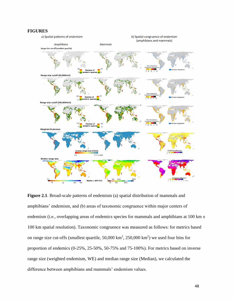
48

FIGURES

Figure 2.1. Broad-scale patterns of endemism (a) spatial distribution of mammals and

amphibians’ endemism, and (b) areas of taxonomic congruence within major centers of

endemism (i.e., overlapping areas of endemics species for mammals and amphibians at 100 km x

100 km spatial resolution). Taxonomic congruence was measured as follows: for metrics based

on range size cut-offs (smallest quartile, 50,000 km2, 250,000 km2) we used four bins for

proportion of endemics (0-25%, 25-50%, 50-75% and 75-100%). For metrics based on inverse

range size (weighted endemism, WE) and median range size (Median), we calculated the

difference between amphibians and mammals’ endemism values.

49

Figure 2.2. Observed vs predicted values of broad-scale patterns of total species endemism

(Log10) for a) amphibians and b) mammals using a cross-continental approach (i.e., models used

the data from all zoogeographic realms from Holt et al. (2013) except one to then predict

endemism on the hold-out continent). We tested four hypotheses (predictors): H1: Climate

50

stability (Climate velocity); H2: Climate seasonality (Seasonality in mean annual temperature);

H3: Climate distinctiveness (in total precipitation, CD_PT); and, H4: Spatial heterogeneity (in

potential evapotranspiration SH_PET)). We tested two metrics of endemism: median range size

and weighted endemism. Results are shown for SAR models.

51

Figure 2.3. Best models predicting broad scale patterns of Endemism (using Median range size

as a metric of endemism) for amphibians (graphs on the left) and mammals (graphs on the right).

a) variance partitioning, b) path analysis and c) Cross-continental validation for best models.

MATS = Seasonality in mean annual temperature; SH_PET = Spatial heterogeneity in potential

evapotranspiration; AET = Actual evapotranspiration; and, Richness = Total species richness.

52

Figure 2.4. Best models predicting broad scale patterns of endemism, using log(Weighted

Endemism) as a metric of endemism for amphibians (graphs on the left) and mammals (graphs

on the right). a) variance partitioning, b) path analysis and c) Cross-continental validation for

best models. Seasonality = Seasonality in mean annual temperature; SH_PET = Spatial

heterogeneity in potential evapotranspiration; AET = Actual evapotranspiration; and, Richness =

Total species richness.

53

CHAPTER 3. Endemic species coverage by the global protected areas network

ABSTRACT

Protected areas (PAs) are one of the main tools for halting habitat degradation and biodiversity

loss worldwide. By 2020, governments have agreed to expand the terrestrial protected area

network from 13% to 17% of the Earth’s surface (Convention on Biological Biodiversity, CBD -

Aichi Target 11, 2010). However, it is not clear to what extent this global strategy has protected

endemic species. As CBD-Aichi Target 11 deadlines approach, we provide a comprehensive

assessment of the impact of terrestrial PAs on endemic species protection. We measure the

relative coverage of endemic species (i.e. species with small range size) by overlapping species

geographic ranges for amphibians, mammals and birds with a global database of PAs (1990-

2016). Then we measure the rate of expansion of the global PA network, and the rate of change

in endemic species coverage.

We found that ~30% of amphibian, ~6% of bird, and ~10% of mammal endemic species

are completely outside PAs. Most endemic species’ ranges intersect the PA network (amphibian

species = 58%; birds = 83%; mammals = 86%), but PAs usually cover less than 50% of the

geographic range. Almost 50% of species outside the PA network are considered threatened

(critically endangered, endangered and vulnerable).

The historic rates of new PAs added every year to the network is between ~6,000 to

~15,000. In contrast, we found that rates of including endemic species within the PA network

have been fairly slow. Historic data shows that annually, additions to the PA network result in 3

(amphibians) to 6 (birds and mammals) endemic species having their entire geographic ranges

covered by the PA network.

54

Based on these trends, it is very unlikely the global PA network will include all endemic

species (14% total endemic species, that is ~1,508 out of 11,274) currently outside the PA

network by 2020. It will require five times the effort made in the last two decades - or a century

if current rates of inclusion persist - to include all endemic species currently outside the PA

network. However, projections also showed that is very likely that some portions of the endemic

species geographic ranges for birds and mammals, but not for amphibians, will be covered by the

future PA network.

INTRODUCTION

One of the major challenges in the 21st century is the conservation and sustainable use of

biological diversity (CBD, 2104). Land use change (LUC) is the leading factor of habitat and

biodiversity loss (Foley et al., 2005; Newbold et al., 2016) and has already degraded more than

60% of ecological systems worldwide (Millennium Ecosystem Assessment, 2005). Protected

areas (PAs) represent a global strategy to halt habitat loss and reduce fragmentation and

overexploitation of natural resources (Butchart et al., 2012; Le Saout et al., 2013). PAs also aim

to protect not only species, but habitats, and ecosystem functions (Duncan et al., 2015) and

services (Parrish et al., 2003). By 2020, countries signatories of the Aichi biodiversity target 11

nations have pledged to increase terrestrial PAs to at least 17% of current Earth surface extent

(CBD, 2010). Preliminary assessments showed some improvements toward this target (2010 =

14% and 2016 = 15.4%) (UNEP-WCMC & IUCN, 2016).

Species with small geographic ranges (an operational definition of endemic species (Jetz

et al., 2004; Ohlemüller et al., 2008a; Pimm et al., 2014)) are of special conservation concern.

Range-restricted species tend to be concentrated in some regions in the world (Lamoreux et al.,

2006), and have been widely used in conservation planning to prioritize highly irreplaceable

55

regions (“hotspots”) and to halt massive biodiversity loss (Myers et al., 2000; Orme et al., 2005;

Brooks et al., 2006). These hotspots represent not only concentrations of young and relictual taxa

(Fjeldså & Lovett, 1997), but topographically complex regions that offer valuable ecosystem

services (Naidoo et al., 2008), and unique biotas in islands and archipielagos (Myers et al.,

2000). Preliminary assessments revealed a big gap in covering hotspots of high endemism within

the global network of PAs, calling the attention to include biodiversity patterns in conservation

planning to increase the likelihood of protecting biological diversity as a whole (Rodrigues et al.,

2004; Joppa et al., 2013). Terrestrial endemic species are constrained to ~25 hotspots in no more

than 1.4% of the land surface and they are severely threatened by loss of habitat (Myers et al.,

2000). Hotspots capture between 44% (Myers et al., 2000) to 59% endemic species in ~17.4

million km2 (Joppa et al., 2013), and the level of protection that the global PA network offer to

these hotspots is likely less than 20% coverage for all three major taxonomic groups:

amphibians, birds and mammals (Jenkins et al., 2013).

Extinction rates are accelerating (Pimm et al., 2014; Ceballos et al., 2015), wild

population still in decline (WWF, 2016), and drivers of species declines show sustained

increases (Butchart et al., 2010). On average, 52 species from vertebrate groups, like

amphibians, birds, and mammals, move one category closer to extinction every year (Hoffmann

et al., 2010). However, conservation efforts, through systematic conservation planning

(Margules & Pressey, 2000; Meir et al., 2004; Pressey et al., 2007), have also made quantifiable

improvements to the status of biological diversity, preventing species from declining toward

extinction (Hoffmann et al., 2010), and facilitating species recovery by reducing habitat loss

(Geldmann et al., 2013). Coordinated efforts to increase PA network extent, such as the Aichi

Biodiversity Target 11 (CBD, 2010), including patterns of biodiversity in conservation

56

planning (Rodrigues et al., 2004), and preventing the extinction of known threatened species

(CBD Aichi Target 12) (CBD, 2010), should pave the way to effectively protect global

biodiversity. In theory, increasing the global network of PAs to 17% has the potential to increase

the average protection of high number of species geographic ranges (totally or partially), but it

will require to require coordinated international efforts (Pouzols et al., 2014). However, it is still

unclear whether this strategy will protect endemic species. Preliminary projections show that

expected extinction rates in hotspots for the next century should be significantly reduced if there

is an increase in the PA network on those hotspots currently unprotected (Pimm & Raven, 2000).

Quantifying the extent to which PAs have protected endemic species over recent decades also

will elucidate the likelihood of protecting endemic species before 2020. Temporal analysis can

be complemented by a spatial analysis, identifying geographic areas, and species to focus

conservation efforts that would help countries to make informed and effective decisions.

Here we ask whether the historical rate of change of endemic species coverage by the

global PA network is likely to protect endemic species by 2020. More specifically, we ask at

present rates of change, when would full endemic coverage be achieved? In addition, we

performed a comprehensive gap analysis to quantify the number of endemic species that are not

covered by the PAs network and their relative threatened status. We provide detailed information

on endemic species and geographic areas for conservation that would help countries to meet

CBD targets.

METHODS

We used global vector distribution maps (only native species = 22,191) for terrestrial mammals

(n = 5,276), and amphibians (n = 6,428) from IUCN (2014), and birds (n = 10,487) from

BirdLife (2016). We used median range size as an operational proxy of endemic species (Pimm

57

et al., 2014), resulting in 11,273 species in total (and mammals = 2,636; amphibians=3,214; and,

birds = 5423). To measure the extinction risk, we used all categories from the IUCN red list

(IUCN, 2014).

We used the world database of PAs (WDPA, n = 214,809) and selected only terrestrial

areas (n = 210,483) worldwide (IUCN & UNEP-WCMC, 2017). Our final PA data set includes

entirely terrestrial PAs (field ‘MARINE’ = 0; n = 200,155) and PAs having some portion of

coastal area (field ‘MARINE’ = 1; n = 10,328). We merged all PA polygons into a single layer

for a total area of 20,518,653 km2, representing 15.2% of the Earth terrestrial surface.

To measure the relative location of each species’ geographic distribution with respect to

the extent of any PA, we overlapped species with the boundaries of PAs. We categorized this

overlap as follows: (i) species geographic ranges that are totally or at least 95% within any PA

boundary (inside); (ii) species whose ranges fall only partially (<95%) within the PA; and, (iii)

species completely outside any PA boundary (outside). For species with ranges only partially

within PAs, we created three categories measuring relative protection afforded by PAs: poor

(>50%), medium (50-75%), and strong proportional range inclusion (75-95% of the species’

range falls within the boundaries of protected areas).

The extent to which endemic species have benefited from progressive expansion of

protected areas networks was measured by counting the number endemic species within PAs

annually over a period of 26 years (1990-2016).

We also assessed how many species are currently threatened (e.g., critically endangered,

endangered, and vulnerable from IUCN categories) but that are found outside the boundaries of

protected areas. To evaluate the degree of land cover change within the geographic range of

endemic species and their relative location with respect to PAs (inside, intersect, and outside

58

PAs), we used the land cover change map from the Millennium Ecosystem Assessment (2005)

(Lepers et al., 2005). This data set shows areas of rapid land-cover change worldwide world

between 1981-2000, synthetizing major forest-cover changes, dry-land degradation, and changes

in human extent. Finally, we summarized our results using terrestrial ecoregions of the world

(Olson et al., 2001) and countries’ administrative divisions from CIESIN - Columbia University

et al. (2011).

All polygons and grids were projected using the World-Behrmann projection to preserve

area across the extent of the analysis. Analyses were performed using ArcGIS (ESRI, 2014) and

R (R Core Team, 2017). The datasets analysed during the current study are available from

citations provided above and results of our analyses can be found at

http://www.macroecology.ca.

RESULTS

Temporal analysis: measurement of the rate of change

Between 1990 and 2016, ~6,000 to ~15,000 PAs were added annually to the global PA network,

but this number has declined in recent years (Figure 1). However, the rates of inclusion of

endemic species within the PA network have been fairly slow in the last two and a half decades.

For instance, the rates of wholly including endemic amphibian species inside the PA network

was about 9 species per year (S/Y), far from doubling the number of endemic species since the

1990 baseline (from 162 to 233; Figure 2). For mammals and birds, the rate at which new

endemic species were added to global PA networks was lower (3 S/Y), leading to a 6-8-fold

increase in numbers of these species whose ranges were fully included in the PA network

(mammals = 10 to 84; and, amphibians = 16 to 99).

59

Completely including all endemic species currently outside the PA network before 2020

(~4 years), within the network, requires a roughly 5-fold increase in rates of new PA

establishment relative to progress observed over the 1990-2016 period. This is especially

challenging for amphibians, a taxon for which 943 species currently fall entirely outside PA

boundaries. In contrast, birds and mammals have fewer species outside the PA network (303 and

262 species, respectively). On the other hand, if conservation objectives are partial inclusion of

endemic species’ ranges, rather than inclusion of species’ entire ranges, then rates of progress are

considerably higher (Figure 2). If current trends persist, most endemic bird and mammal species

currently outside PAs will be receiving at least partial protection within PA boundaries by 2020.

In contrast, rates of partial inclusion for endemic amphibians that had no prior presence within

PAs are lower (Figure 2). Challenges also remain in protecting the whole extent of these endemic

species, safeguarding single areas between 10 Km2 to 10,000 Km2. The average extent of PAs

added to the network is far smaller (~2 orders of magnitude) than the size of these species’

geographical ranges (Figure 3).

Coverage

We found that only 3% of the geographic ranges for all major terrestrial vertebrates are

completely inside the PA network (~6% of endemic species) and around 7% (~14% of endemic

species) are entirely outside the PA network (Table 1, Figure 4a). For amphibians, almost 30% of

all endemic species are not covered by any PA, and 58% of species are partially covered by the

PA network (Table 1). Nearly 80% of the geographic ranges for birds and mammals are

somewhat covered by the PA network.

Extinction risk

60

Depending on taxon, between 50-60% of endemic species inside PAs are considered threatened

(i.e., aggregating IUCN red list categories: critically endangered, endangered and vulnerable).

Surprisingly, the number of endemic species threatened and not included (outside) by the PA

network is slightly lower (between 40-50%) than endemic species inside the PA network (Figure

4b). Birds showed the highest number of endemic species threatened inside PAs and the lowest

number of endemic species threatened in partially covered (intersect) by PAs.

Extinct species

We found that the geographic range of a high number of endemic bird species that went extinct

(n = 44; using IUCN status = ‘Extinct’) were not covered by the PA network (Figure 4c).

Numbers for mammals and amphibians were comparative lower (2 and 6, respectively).

Countries

Endemic species that are not currently covered by the PA network (outside) are concentrated in

some countries (Figure 5), including for amphibians: Brazil, Mexico, Colombia, and Peru; and

Papua New Guinea; for birds: Bolivia, Australia and Costa Rica; and, for mammals: Indonesia,

Argentina and Papua New Guinea (Table 2). Papua New Guinea harbors the highest number of

endemic species for each of the three taxonomic groups.

Ecoregions

Most amphibians outside protected terrestrial areas are concentrated in the ecological regions

along the tropical Andes and in New Guinea, while areas with high concentrations of endemic

bird species are particularly among islands in the Pacific. Endemic mammals are especially

concentrated in the dry Chaco region in southern South America (Figure 6).

Land cover/land use

61

For birds and amphibians, the dominant land cover within the geographical ranges of endemic

species completely inside PAs is primary forest (Figure 7). In contrast, secondary forest and

pastures dominate the geographic ranges of mammals’ endemic species within the PA network.

Geographic ranges of endemic species for birds and mammals outside the PA network are

mainly cover by pastures and secondary forest, and by primary forest for amphibians (Figure 7).

For species’ geographic ranges intersecting the PA network, land use/land cover changes take

various forms (i.e. from urban areas to primary forest).

DISCUSSION

The rate of change in endemic species coverage has been very slow in the last two and half

decades (1990-2016), making if very unlikely, if the rate is maintained, that the world’s endemic

species can be wholly included within protected areas 2020. Between 1990 and 2016, the rate of

endemic species coverage was very low (3 to 9 species per year, depending on the taxonomic

group). So, maintaining these rates of change, more than a century will be required to include

~1508 endemic species currently outside the PA network. Projections based on historic data

showed that is very likely that some portions of the geographic ranges of birds and mammals’

endemic but not amphibians species will be covered by the future PA network.

Despite the slow historic rate of endemic species coverage, the Aichi target that nations

are working toward represent an opportunity to include and protect high numbers of endemic

species within the global PA network. An optimistic scenario could be including the total

number of geographic ranges of endemic species currently outside the PA network (n=1,508)

within it. Expanding the PA network to include all these species before 2020 will require five

times the effort made in the last two decades. It will be likely because the historic rate of new

PAs added every year is between ~6,000 to ~15,000. This will fill the gap and lack of protection

62

of species with small range sizes and associated niches (Gray et al., 2016). However, it will

require an effort to leveraging financial resources, encouraging political will and trading-off with

other biodiversity and ecological features to include these species.

If protecting endemic species is worthwhile because they represent a group of desirable

and strategic features in biodiversity conservation (Myers et al., 2000; Orme et al., 2005; Brooks

et al., 2006; Naidoo et al., 2008), then international community (local, regional and national

governments, international cooperation agencies, NGOs, etc.) might focus on prioritizing them to

be part of the PA network by 2020. So, expanding the PA network to cover the full extent of

endemic species currently outside the PA network will protect almost 14% total endemic species

(1,508 out of 11,274). For amphibians, it will impact the most, around 30% of total endemic

species will be covered (943).

Systematic conservation planning is needed to solve some issues emerging from different

scenarios. For example, it is likely that many new species, with small geographic ranges, remain

to be describe (Scheffers et al., 2012). New discoveries are more likely to occur for amphibians

than for others groups (Pimm et al., 2010); and some estimates, for other dominant groups such

as flowering plants, indicate a high percentage (~15%) of species that still likely undiscovered

(Joppa et al., 2011). Some areas may be “hotspots” of endemism for particular or multiple taxa,

so targeting such hotspots for protection would lead to substantial progress in endemic species

conservation. Under current trend it is expected that some endemic species of mammals and

birds (and less likely amphibians) will be covered in some way for a PA in the next 4 years, so it

will be a priority to evaluate the effectiveness of this partial protection. Challenges also emerge

in protecting the whole extent of each endemic species, because it requires safeguarding single

areas between 10 Km2 to 10,000 Km2 and restoring natural habitats which have dramatically

63

changed in land cover use (from forest to secondary forest and pastures), specially for mammals

and birds’ geographic distributions.

One of the assumptions in conservation is that creating PAs will secure species and

associated ecosystem functions. We evaluate only one dimension of biodiversity that can offer

quantitative information of the effectiveness of the PAs (Chape et al., 2005). A comprehensive

assessment of biodiversity, oriented to set global conservation priorities must also consider other

facets and metrics (Brum et al., 2017; Pollock et al., 2017), such as rarity (Possingham &

Wilson, 2005), and other dimension of biodiversity (Hoekstra et al., 2005) and ecosystem

services (Turner et al., 2007). However, the expansion PA network covering the extent of species

with small range size seems to offer not only highly cost-effective protection of areas of high

biodiversity (Balmford et al., 2002; Venter et al., 2014), but sustained provision of ecosystems

services basic for human activities.

Areas within and surrounding PAs have experienced land change use and exploitation of

natural resources, resulting in biodiversity loss (Laurance et al., 2011) and degradation of

ecosystem services (Foley et al., 2005), such as climate and air quality regulation. We found that

areas outside the PA network, harboring endemic species, have experience changes in land cover

use (from forest to secondary forest, pastures and crops); especially for mammals and birds’

geographic distributions. LUC projections also show that this trend of ecosystems degradation

will continue in the next two decades (Pouzols et al., 2014). In fact, habitat fragmentation has

been associated as a major driver for mammal extinction risk and endemic species have suffered

significant losses of critical habitat from within their geographic range (Crooks et al., 2017).

Land use change in countries with particularly high diversity (e.g., Indonesia, Papua New Guinea

and Colombia) accelerates extinctions and the erosion of other aspects of biological diversity,

64

such as phylogenetic diversity (Chaudhary et al., 2018). Expanding the PA network rapidly into

remaining intact habitats would significantly improve conservation prospects for tropical species

(Gibson et al., 2011; Dinerstein et al., 2017; Watson & Venter, 2017).

Expanding PAs to areas where endemic species are currently unprotected will require

restoration efforts, whether active or passive, that recover habitat quality (Birch et al., 2010). We

showed that almost 50% of the endemic species outside the PA network are threatened (i.e.,

critically endangered, endangered and vulnerable) and at least 180 species are reportedly extinct

based on IUCN red lists, most of them birds. This risk factor can increase if detailed spatial data

are incorporated within the analysis (Ocampo-Peñuela et al., 2016) and environmental stressors

persist. Biological diversity has been eroded at rates never experienced (Ceballos et al., 2015)

and range-restricted species have lost their historic range area due to intensive human activities

(Ceballos & Ehrlich, 2002). Moreover, vertebrate population has showed 25% average decline in

abundance (Dirzo et al., 2014).and habitat loss and fragmentation may compromise maintenance

of healthy populations and species stocks in the future (Brooks & Balmford, 1996; Brooks et al.,

1999). Reducing extinction risk of endemic species effectively requires also targeting the places

very precisely in the landscape (Akasaka et al., 2017).

Endemic species outside the PA network are located mainly in areas previously identified

as biodiversity hotspots (Myers et al., 2000): the Andes, Choco, Pacific Islands (e.g., New

Guinea, Solomon), Mesoamerica, Dry Chaco and Atlantic forests. And, they also occupy

ecoregions where habitat conversion exceeds habitat protection (Hoekstra et al., 2005) and

species losses may most likely occur (Manne et al., 1999). Within these ecoregions, it is

necessary to refine conservation priorities (Jenkins et al., 2010) and monitoring PAs (Nagendra

65

et al., 2013) using new technological tools such as remote sensing (Rose et al., 2015; Pettorelli et

al., 2016).

Persistence of species, habitats and ecosystems services depends not only on including

biological and ecological factors but on coordinating and translating generalized, global drives

toward international conservation agreements into achievable goals within nations and the

societies that comprise them (Pouzols et al., 2014). Global, regional and local realities may

emerge in the attempt to implement conservation goals. Reconciling conservation and

development targets may increase land use efficiency and minimize habitat and biodiversity loss

(Lambin & Meyfroidt, 2011). Similarly, attempts to combine and reconcile interests of different

stakeholders into national and local policies could help to minimize poverty, redefine local

economic development and protect biological diversity (Adams et al., 2004; Naughton-Treves et

al., 2005; Berkes, 2007; Palmer & Di Falco, 2012; Mishra et al., 2017).

Protecting endemic species requires coordinated efforts to expand a large and dispersed

network of PAs and implement regional conservation management to mitigate environmental

stressors and enhance biological and ecological processes (Ceballos et al., 2005). Increasing the

number of PAs globally must also be accompanied by reducing PA removal from the global

network (Lewis et al., 2017). Coordinating global targets, governments efforts and local

implementation require a new aggressive campaign to protect biodiversity and ecosystem

services. New PAs and areas buffering them should be managed by national and regional

agencies in coordination with local communities and NGOs. Local stakeholders could adopt

these areas and obtain tangible social and economic benefits.

Aichi target 11 offers a unique opportunity to include all endemic species currently

outside the global PA network within it. However, historical data showed that current rates of

66

change in including endemic species are very slow. So, a call to the international community

(local, regional and national governments, international agencies, NGOs, etc.) is made to focus

and establish an international strategy to include more than 1500 endemic vertebrate species

(amphibians, birds and mammals) within the current PA network before 2020. It will preserve

not only a substantial number of species but also habitats and ecosystem functions and services.

ACKNOWLEDGEMENTS

JZ is grateful to the University of Ottawa for Graduate Admission Scholarship support. JZ would

like to thank Peter Soroye for his comments and editing of this manuscript.

67

TABLES

Table 3.1. Number of endemic species that overlap (inside or intersect) or not (outside) with Protected Areas (PAs). Values in

parenthesis represent the proportion (%) of species in each category within that taxon. Endemic species are based on median range size.

“Inside” indicates that polygons of species’ ranges are 95% or more contained within the PA network; “outside” indicates species ranges

totally outside the PA network; “intersect” indicates overlap of species geographic ranges with the PA network in three categories:

between 75% - 95%, 50% - 75% and less than 50%.

Species location with respect to Protected Terrestrial Areas

Taxon Total species Endemic species Inside Intersect Outside

75% - 95% 50%-75% < 50%

Amphibians1 6,428 3,214

(50%)

395

(6%)

243

(4%)

344

(5%)

1,289

(20%)

943

(15%)

Birds2 10,487 5,423

(52%)

84

(1%)

133

(1%)

322

(3%)

4,581

(38%)

303

(3%)

Mammals3 5,276 2,636

(50%)

99

(2%)

126

(2%)

211

(4%)

1,938

(37%)

262

(5%)

Total species 22,191 11,274

(51%)

578

(3%)

502

(2%)

877

(4%)

7,808

(35%)

1,508

(7%) Cut-off median range size: 1 Amphibians = 4,478 Km2 2 Birds = 421,151 Km2

3 Mammals = 182,722 Km2

68

Table 3.2. Top 20 countries harboring the highest number of endemic species outside the protected terrestrial areas (PAs) network for

amphibians, birds and mammals. Countries holding high numbers of endemic species for: three taxonomic groups (red), two taxa

(blue), and one taxon (black).

Country Amphibians Country Birds

Country Mammals

1 Papua New Guinea 99

Bolivia 239

Indonesia 33

2 Brazil 93

Australia 160

Argentina 24

3 Mexico 88

Costa Rica 117

Papua New Guinea 22

4 Peru 84

Burundi 74

Mexico 18

5 Colombia 74

United States of America 68

Philippines 12

6 India 57

Belize 63

Solomon Islands 12

7 Ecuador 56

Bhutan 57

India 10

8 Indonesia 42

Guatemala 54

Madagascar 10

9 China 31

Venezuela 51

Ethiopia 8

10 Haiti 28

Brunei Darussalam 47

Sudan 8

11 Cameroon 25

Solomon Islands 44

China 7

12 Bolivia 16

French Polynesia 43

Congo, Democratic Republic 7

13 Argentina 15

Cameroon 41

Somalia 7

14 Congo, Democratic Republic 15

Papua New Guinea 40

Iran 5

15 Guatemala 15

Ethiopia 39

Russia 4

16 Venezuela 15

Cuba 35

Turkey 4

17 United Rep. of Tanzania 14

Dominican Republic 34

Angola 3

18 Angola 13

Chile 33

Cuba 3

19 Chile 13

Jamaica 33

Federated State of Micronesia 3

20 Madagascar 13

Sri Lanka 33

South Africa 3

69

FIGURES

Figure 3.1. Number of protected terrestrial areas (PAs) included in the global network since

1990 (thick black line), and projections to include all endemic species currently outside the PA

network (n = 1,580, black thin line) by 2020. Two additional projections are calculated using two

rates of change of endemic species coverage: low rate, purple dashed line; and high rate, green

dashed line. Projected trends of PA coverage by 2020, using minimum (grey dashed line) and

maximum (thin black line) historical rates.

70

Figure 3.2. Number of endemic species that are inside (blue line) or intersect (red line) protected terrestrial areas (PAs) for a)

amphibians, b) birds and c) mammals. Historic trend represented by thick lines. Two projections aimed to include endemic species

within the PA network: using total number of endemic species outside current (2016) PA network (thin line) and using the historic rate

of change for species coverage (dotted line).

71

Figure 3.3. Extent of protected terrestrial (PAs) areas (yellow) and geographic range size extent

endemic species outside the PA network for amphibians (green), birds (red) and mammals

(blue).

72

73

74

Figure 3.4. Coverage of endemic species by protected terrestrial areas (PAs, data 1990-2016). a)

Total endemic species; b) Threatened endemic species (aggregated IUCN categories: Critically

endangered, Endangered and Vulnerable) from total; and, c) Extinct species. Species geographic

ranges that intersect any PA (categories in blues hues) where subdivided according to their

percentage of overlap with PAs’ extent (i.e., 75% - 95%, 50% - 75% and less than 50% of

overlap). Notice that species that overlapped more than 95% with any PAs where considered

inside PAs.

75

Figure 3.5. Number of endemic species outside Protected Areas (PAs) per country for a)

amphibians, b) birds and c) mammals.

76

77

78

Figure 3.6. Ecoregions and number of endemic species completely outside protected terrestrial

areas for a) amphibians, b) birds and c) mammals. Bars represent a sample of ecoregions with

highest number of endemic species.

79

80

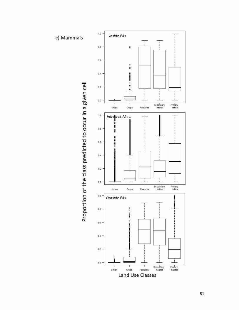
81

82

Figure 3.7. Proportion of the class predicted to occur within a given cell within the extent of the

species geographic range (i.e., inside, outside or intersect the protected area network, PAs); for a)

amphibians, b) birds, and c) mammals.

83

GENERAL CONCLUSION

My thesis attempted to test some hypotheses that can explain broad-scale patterns of

species endemism, and to inform conservation planning about the likelihood of protecting

endemic species under a global conservation initiative (Aichi target 11, Convention of Biological

Diversity).

I found that thermal barriers proposed to characterize differences between tropical and

temperate realms are not accurate. Thermal barriers might be more complex than a latitudinal

climate gradient. I also found that hypotheses tested here failed to provide a reliable explanation

of macroecological patterns. In terms of conservation, I found that it is very unlikely to protect

all endemic species at the present rates endemics are being covered by PAs.

In Chapter 1, I found that thermal barriers between low and high elevation areas, initially

proposed to be unique to tropical environments, are comparably strong in some temperate

regions, particularly along the western slopes of North American dividing ranges. I also found

that biotic similarity for both mammals and amphibians decreases between sites that are

separated by elevation-related thermal barriers. That is, the stronger the thermal barrier

separating pairs of sites across the latitudinal gradient, the lower the similarity of their species

assemblages. Thermal barriers explain 10-35% of the variation in latitudinal gradients of biotic

similarity, effects that were stronger in the comparisons of sites at high elevations. Thermal

barriers are weaker or absent at low elevations (Wright et al. 2009, Salisbury et al. 2012), and

our results cannot readily explain variation in species assemblages within such areas. So,

processes intrinsic to the classic ‘mountain passes’ hypothesis (Janzen 1967) appear to contribute

in some way to the origins and maintenance of broad-scale gradients of biological diversity.

However, other factors, whether historical or contemporary, must be the main drivers of

84

gradients of biological diversity. My findings also have significant implications. If mountains

passes are also high in temperate regions, it is unlikely that the mechanism proposed by Janzen

(1967) may explain broad-scale patterns of total species richness, as this hypothesis predicts a

significant peak of richness in some temperate regions in western North America which is not

supported by empirical evidence (Currie, 2017). Based on this, we should reject Janzen’s

hypothesis and its main mechanism as a candidate to explain broad-scale patterns of total species

richness.

In Chapter 2, I found that there is no empirical reason, from the standpoint of model

fitting, parameter estimates and model validation, to claim that any tested process, individually

or in combination, creates and maintains global patterns of endemism. Although, I found

significant relationships, they failed the stronger test of a causal relationship: accurate prediction.

Although all relationships are statistically significant, most of the variance remains unexplained,

and cross-continental tests of spatial models did not accurately predict observed patterns of

endemism in spatially independent zoogeographic realms. This suggests that regression models

between predictors and endemism do not capture fundamental processes that generate endemism.

That the effect of richness almost disappeared in some models, suggests that patterns of

endemism are not driven by the same variables as total richness. Patterns of endemism were not

consistently related to climatic velocity, suggesting that early correlations in some places

probably reflect collinearity with topography instead. Local combinations of biotic and abiotic

conditions that are essentially unpredictable by any macroecological approach might be

responsible for patterns of endemism.

In Chapter 3, I found that 30% of amphibians, 6% of birds and 10% of mammals’

endemic species are completely outside Protected Areas (PAs). Almost 50% of species outside

85

PAs, and partially covered by the PA network, are considered threatened (critically endangered,

endangered and vulnerable). Between 1990 and 2016, 3 to 6 endemic species have been

completely covered every year by the PA network (# included amphibian species = 162 to 233;

mammals = 10 to 84; and, amphibians = 16 to 99). Based on these trends, including all endemic

species currently outside the PA network completely within it is very unlikely by 2020.

However, projections also showed that is very likely that some portions of all endemic species’

geographic ranges for birds and mammals, but not for amphibians, will be covered by the 2020

PA network. If protecting endemic species is worthwhile, because they represent a strategic

feature in biodiversity conservation, then international community and local governments might

focus on prioritizing them to be part of the PA network by 2020. Expanding the PA network to

cover the full extent of endemic species currently outside the PA network will protect almost

14% total endemic species (1,508 out of 11,274), safeguarding not only endemic species but the

habitats, historical processes, and ecosystem services associated with them. Ecoregions in

tropical Andes, Mesoamerica, Pacific Islands (e.g., New Guinea, Solomon), Dry Chaco, and

Atlantic forests are major priorities. Challenges remain in protecting the whole extent of each

endemic species, because it requires safeguarding single areas between 10 Km2 to 10,000 Km2,

and restoring natural habitats which have dramatically changed in land cover use (from forest to

secondary forest and pastures), especially for mammals’ and birds’ geographic distributions.

Finally, my main contribution to this research area is clearly rejecting these hypotheses

from potential candidates that may explain biodiversity patterns. By removing them, I advance in

this field and open possibilities to test new ideas and gather new evaluate their mechanisms. By

investigating rates of endemic species inclusion in PAs, I provide detailed information and

86

methodologies that can help countries to strategically conserve biodiversity and meet CBD target

requirements.

87

REFERENCES

Adams, W.M., Aveling, R., Brockington, D., Dickson, B., Elliott, J., Hutton, J., Roe, D., Vira, B.

& Wolmer, W. (2004) Biodiversity conservation and the eradication of poverty. Science,

306, 1146-1149.

Addo-Bediako, A., Chown, S.L. & Gaston, K.J. (2000) Thermal tolerance, climatic variability

and latitude. Proc. Biol. Sci. B, 267, 739-745.

Akasaka, M., Kadoya, T., Ishihama, F., Fujita, T. & Fuller, R.A. (2017) Smart Protected Area

Placement Decelerates Biodiversity Loss: A Representation-extinction Feedback Leads

Rare Species to Extinction. Conservation Letters, 10, 539-546.

Anderson, S. (1994) Area and Endemism. The Quarterly Review of Biology, 69, 451-471.

Angilletta, M.J. (2009) Thermal adaptation : a theoretical and empirical synthesis. Oxford

University Press, Oxford.

Ashcroft, M.B. (2010) Identifying refugia from climate change. Journal of Biogeography, 37,

1407-1413.

Balmford, A., Bruner, A., Cooper, P., Costanza, R., Farber, S., Green, R.E., Jenkins, M.,

Jefferiss, P., Jessamy, V. & Madden, J. (2002) Economic reasons for conserving wild

nature. Science, 297, 950-953.

Bellard, C., Bertelsmeier, C., Leadley, P., Thuiller, W. & Courchamp, F. (2012) Impacts of

climate change on the future of biodiversity. Ecol Lett, 15, 365-77.

Bellard, C., Leclerc, C., Leroy, B., Bakkenes, M., Veloz, S., Thuiller, W. & Courchamp, F.

(2014) Vulnerability of biodiversity hotspots to global change. Global Ecology and

Biogeography, 23, 1376-1386.

88

Belmaker, J. & Jetz, W. (2011) Cross-scale variation in species richness–environment

associations. Global Ecology and Biogeography, 20, 464-474.

Berger, A. (1988) Milankovitch theory and climate. Reviews of Geophysics, 26, 624-657.

Berkes, F. (2007) Community-based conservation in a globalized world. Proceedings of the

National Academy of Sciences, 104, 15188-15193.

Bini, M.L., Diniz-Filho, J.A.F., Rangel, T.F.L.V.B., Akre, T.S.B., Albaladejo, R.G.,

Albuquerque, F.S., Aparicio, A., Araújo, M.B., Baselga, A., Beck, J., Isabel Bellocq, M.,

Böhning-Gaese, K., Borges, P.A.V., Castro-Parga, I., Khen Chey, V., Chown, S.L., De

Marco, J.P., Dobkin, D.S., Ferrer-Castán, D., Field, R., Filloy, J., Fleishman, E., Gómez,

J.F., Hortal, J., Iverson, J.B., Kerr, J.T., Daniel Kissling, W., Kitching, I.J., León-Cortés,

J.L., Lobo, J.M., Montoya, D., Morales-Castilla, I., Moreno, J.C., Oberdorff, T., Olalla-

Tárraga, M.Á., Pausas, J.G., Qian, H., Rahbek, C., Rodríguez, M.Á., Rueda, M.,

Ruggiero, A., Sackmann, P., Sanders, N.J., Carina Terribile, L., Vetaas, O.R. & Hawkins,

B.A. (2009) Coefficient shifts in geographical ecology: an empirical evaluation of spatial

and non-spatial regression. Ecography, 32, 193-204.

Birch, J.C., Newton, A.C., Aquino, C.A., Cantarello, E., Echeverría, C., Kitzberger, T.,

Schiappacasse, I. & Garavito, N.T. (2010) Cost-effectiveness of dryland forest restoration

evaluated by spatial analysis of ecosystem services. Proceedings of the National

Academy of Sciences, 107, 21925-21930.

BirdLife (2016) Bird species distribution maps of the world. Version 6.0. Available at

http://datazone.birdlife.org/species/requestdis. Accessed March, 2017. In. BirdLife

International and Handbook of the Birds of the World

89

Bonebrake, T.C. (2013) Conservation implications of adaptation to tropical climates from a

historical perspective. Journal of Biogeography, 40, 409-414.

Brooks, T. & Balmford, A. (1996) Atlantic forest extinctions. Nature, 380, 115.

Brooks, T.M., Pimm, S.L. & Oyugi, J.O. (1999) Time lag between deforestation and bird

extinction in tropical forest fragments. Conservation Biology, 13, 1140-1150.

Brooks, T.M., Mittermeier, R.A., da Fonseca, G.A., Gerlach, J., Hoffmann, M., Lamoreux, J.F.,

Mittermeier, C.G., Pilgrim, J.D. & Rodrigues, A.S. (2006) Global biodiversity

conservation priorities. Science, 313, 58-61.

Brown, C., Burslem, D., Illian, J., Bao, L., Brockelman, W., Cao, M., Chang, L., Dattaraja, H.,

Davies, S. & Gunatilleke, C. (2013) Multispecies coexistence of trees in tropical forests:

spatial signals of topographic niche differentiation increase with environmental

heterogeneity. Proceedings of the Royal Society of London B: Biological Sciences, 280,

20130502.

Brum, F.T., Graham, C.H., Costa, G.C., Hedges, S.B., Penone, C., Radeloff, V.C., Rondinini, C.,

Loyola, R. & Davidson, A.D. (2017) Global priorities for conservation across multiple

dimensions of mammalian diversity. Proceedings of the National Academy of Sciences,

Brumfield, R.T. & Capparella, A.P. (1996) Historical diversification of birds in northwestern

South America: A molecular perspective on the role of vicariant events. Evolution, 50,

1607-1624.

Buckley, L.B. & Jetz, W. (2008) Linking global turnover of species and environments.

Proceedings of the National Academy of Sciences of the United States of America, 105,

17836-17841.

90

Buckley, L.B., Miller, E.F. & Kingsolver, J.G. (2013) Ectotherm thermal stress and

specialization across altitude and latitude. Integrative and Comparative Biology, 53, 571-

581.

Butchart, S.H., Scharlemann, J.P., Evans, M.I., Quader, S., Arico, S., Arinaitwe, J., Balman, M.,

Bennun, L.A., Bertzky, B. & Besancon, C. (2012) Protecting important sites for

biodiversity contributes to meeting global conservation targets. PLoS ONE, 7, e32529.

Butchart, S.H.M., Walpole, M., Collen, B., van Strien, A., Scharlemann, J.P.W., Almond,

R.E.A., Baillie, J.E.M., Bomhard, B., Brown, C., Bruno, J., Carpenter, K.E., Carr, G.M.,

Chanson, J., Chenery, A.M., Csirke, J., Davidson, N.C., Dentener, F., Foster, M., Galli,

A., Galloway, J.N., Genovesi, P., Gregory, R.D., Hockings, M., Kapos, V., Lamarque, J.-

F., Leverington, F., Loh, J., McGeoch, M.A., McRae, L., Minasyan, A., Morcillo, M.H.,

Oldfield, T.E.E., Pauly, D., Quader, S., Revenga, C., Sauer, J.R., Skolnik, B., Spear, D.,

Stanwell-Smith, D., Stuart, S.N., Symes, A., Tierney, M., Tyrrell, T.D., Vié, J.-C. &

Watson, R. (2010) Global Biodiversity: Indicators of Recent Declines. Science, 328,

1164-1168.

Cadena, C.D., Kozak, K.H., Gomez, J.P., Parra, J.L., McCain, C.M., Bowie, R.C.K., Carnaval,

A.C., Moritz, C., Rahbek, C., Roberts, T.E., Sanders, N.J., Schneider, C.J., VanDerWal,

J., Zamudio, K.R. & Graham, C.H. (2012) Latitude, elevational climatic zonation and

speciation in New World vertebrates. Proc. Biol. Sci. B, 279, 194-201.

Cadotte, M.W. (2006) Dispersal and species diversity: A Meta‐Analysis. American Naturalist,

167, 913-924.

91

CBD (2010) Decision X/2, The strategic plan for biodiversity 2011–2020 and the Aichi

Biodiversity Targets, Nagoya, Japan, 18 to 29 October 2010. Available at

http://www.cbd.int/decision/cop/default.shtml?id=13164 (2010).

CBD (2104) Global Biodiversity Outlook 4 - Summary and Conclusions. Secretariat of the

Convention on Biological Diversity. In, p. 20, Montréal.

Ceballos, G. & Ehrlich, P.R. (2002) Mammal population losses and the extinction crisis. Science,

296, 904-907.

Ceballos, G., Ehrlich, P.R., Soberón, J., Salazar, I. & Fay, J.P. (2005) Global Mammal

Conservation: What Must We Manage? Science, 309, 603-607.

Ceballos, G., Ehrlich, P.R., Barnosky, A.D., García, A., Pringle, R.M. & Palmer, T.M. (2015)

Accelerated modern human–induced species losses: Entering the sixth mass extinction.

Science Advances, 1

Chao, A., Chazdon, R.L., Colwell, R.K. & Shen, T.J. (2005) A new statistical approach for

assessing similarity of species composition with incidence and abundance data. Ecology

Letters, 8, 148-159.

Chape, S., Harrison, J., Spalding, M. & Lysenko, I. (2005) Measuring the extent and

effectiveness of protected areas as an indicator for meeting global biodiversity targets.

Philosophical Transactions of the Royal Society B: Biological Sciences, 360, 443-455.

Chaudhary, A., Pourfaraj, V. & Mooers, A.O. (2018) Projecting global land use-driven

evolutionary history loss. Diversity and Distributions, 24, 158-167.

Chesson, P. (2000) General theory of competitive coexistence in spatially-varying environments.

Theoretical population biology, 58, 211-237.

92

CIESIN - Columbia University, International Food Policy Research Institute - IFPRI, The World

Bank & Centro Internacional de Agricultura Tropical - CIAT (2011) Global Rural-Urban

Mapping Project, Version 1 (GRUMPv1): National Administrative Boundaries. . In.

NASA Socioeconomic Data and Applications Center (SEDAC), Palisades, NY.

Colwell, R.K. (2013) EstimateS: Statistical estimation of species richness and shared species

from samples. Version 9. User's Guide and application published at:

http://purl.oclc.org/estimates.

Coristine, L.E., Robillard, C.M., Kerr, J.T., O'Connor, C.M., Lapointe, D. & Cooke, S.J. (2014)

A conceptual framework for the emerging discipline of conservation physiology.

Conservation Physiology, 2

Crisp, M.D., Laffan, S., Linder, H.P. & Monro, A. (2001) Endemism in the Australian flora.

Journal of Biogeography, 28, 183-198.

Crooks, K.R., Burdett, C.L., Theobald, D.M., King, S.R.B., Di Marco, M., Rondinini, C. &

Boitani, L. (2017) Quantification of habitat fragmentation reveals extinction risk in

terrestrial mammals. Proceedings of the National Academy of Sciences,

Currie, D.J. (1991) Energy and large-scale patterns of animal-speceis and plant-species richness.

American Naturalist, 137, 27-49.

Currie, D.J. (2017) Mountain passes are higher not only in the tropics. Ecography, 40, 459-460.

Currie, D.J., Mittelbach, G.G., Cornell, H.V., Field, R., Guegan, J.F., Hawkins, B.A., Kaufman,

D.M., Kerr, J.T., Oberdorff, T., O'Brien, E. & Turner, J.R.G. (2004) Predictions and tests

of climate-based hypotheses of broad-scale variation in taxonomic richness. Ecology

Letters, 7, 1121-1134.

93

De Frenne, P., Rodríguez-Sánchez, F., Coomes, D.A., Baeten, L., Verstraeten, G., Vellend, M.,

Bernhardt-Römermann, M., Brown, C.D., Brunet, J., Cornelis, J., Decocq, G.M.,

Dierschke, H., Eriksson, O., Gilliam, F.S., Hédl, R., Heinken, T., Hermy, M., Hommel,

P., Jenkins, M.A., Kelly, D.L., Kirby, K.J., Mitchell, F.J.G., Naaf, T., Newman, M.,

Peterken, G., Petřík, P., Schultz, J., Sonnier, G., Van Calster, H., Waller, D.M., Walther,

G.-R., White, P.S., Woods, K.D., Wulf, M., Graae, B.J. & Verheyen, K. (2013)

Microclimate moderates plant responses to macroclimate warming. Proceedings of the

National Academy of Sciences,

Deutsch, C.A., Tewksbury, J.J., Huey, R.B., Sheldon, K.S., Ghalambor, C.K., Haak, D.C. &

Martin, P.R. (2008) Impacts of climate warming on terrestrial ectotherms across latitude.

Proceedings of the National Academy of Sciences of the United States of America, 105,

6668-6672.

Dillon, M.E., Wang, G. & Huey, R.B. (2010) Global metabolic impacts of recent climate

warming. Nature, 467, 704-706.

Dimitrov, D., Nogues-Bravo, D. & Scharff, N. (2012) Why do tropical mountains support

exceptionally high biodiversity? The Eastern Arc mountains and the drivers of

Saintpaulia diversity. PLoS ONE, 7, e48908.

Dinerstein, E., Olson, D., Joshi, A., Vynne, C., Burgess, N.D., Wikramanayake, E., Hahn, N.,

Palminteri, S., Hedao, P. & Noss, R. (2017) An ecoregion-based approach to protecting

half the terrestrial realm. BioScience, 67, 534-545.

Dirzo, R., Young, H.S., Galetti, M., Ceballos, G., Isaac, N.J.B. & Collen, B. (2014) Defaunation

in the Anthropocene. Science, 345, 401-406.

94

Dormann, C.F., Elith, J., Bacher, S., Buchmann, C., Carl, G., Carré, G., Marquéz, J.R.G.,

Gruber, B., Lafourcade, B., Leitão, P.J., Münkemüller, T., McClean, C., Osborne, P.E.,

Reineking, B., Schröder, B., Skidmore, A.K., Zurell, D. & Lautenbach, S. (2013)

Collinearity: a review of methods to deal with it and a simulation study evaluating their

performance. Ecography, 36, 27-46.

Duncan, C., Thompson, J.R. & Pettorelli, N. (2015) The quest for a mechanistic understanding of

biodiversity–ecosystem services relationships. Proc. R. Soc. B (ed by, p. 20151348.

Dynesius, M. & Jansson, R. (2000) Evolutionary consequences of changes in species'

geographical distributions driven by Milankovitch climate oscillations. Proceedings of

the National Academy of Sciences, 97, 9115-9120.

ESRI (2014) ArcGIS Desktop 10.2. Redlands, CA: Environmental Systems Research Institute.,

Fjeldså, J. & Lovett, J. (1997) Geographical patterns of old and young species in African forest

biota: the significance of specific montane areas as evolutionary centres. Biodiversity &

Conservation, 6, 325-346.

Fjeldså, J., Lambin, E. & Mertens, B. (1999) Correlation between endemism and local

ecoclimatic stability documented by comparing Andean bird distributions and remotely

sensed land surface data. Ecography, 22, 63-78.

Fjeldså, J., Bowie, R.C.K. & Rahbek, C. (2012) The Role of Mountain Ranges in the

Diversification of Birds. Annual Review of Ecology, Evolution, and Systematics, 43, 249-

265.

Fjeldså, J., Ehrlich, D., Lambin, E. & Prins, E. (1997) Are biodiversity 'hotspots' correlated with

current ecoclimatic stability? A pilot study using the NOAA-AVHRR remote sensing

data. Biodiversity and Conservation, 6, 401-422.

95

Foley, J.A., DeFries, R., Asner, G.P., Barford, C., Bonan, G., Carpenter, S.R., Chapin, F.S., Coe,

M.T., Daily, G.C., Gibbs, H.K., Helkowski, J.H., Holloway, T., Howard, E.A., Kucharik,

C.J., Monfreda, C., Patz, J.A., Prentice, I.C., Ramankutty, N. & Snyder, P.K. (2005)

Global Consequences of Land Use. Science, 309, 570-574.

Francis, A.P. & Currie, D.J. (2003) A globally consistent richness-climate relationship for

angiosperms. American Naturalist, 161, 523-536.

Gaston, K.J. (1998) Ecology: Rarity as double jeopardy. Nature, 394, 229-230.

Gaston, K.J. (2003) The structure and dynamics of geographic ranges. Oxford University Press

on Demand.

Geldmann, J., Barnes, M., Coad, L., Craigie, I.D., Hockings, M. & Burgess, N.D. (2013)

Effectiveness of terrestrial protected areas in reducing habitat loss and population

declines. Biological Conservation, 161, 230-238.

Ghalambor, C.K., Huey, R.B., Martin, P.R., Tewksbury, J.J. & Wang, G. (2006) Are mountain

passes higher in the tropics? Janzen's hypothesis revisited. Integrative and Comparative

Biology, 46, 5-17.

Gibson, L., Lee, T.M., Koh, L.P., Brook, B.W., Gardner, T.A., Barlow, J., Peres, C.A.,

Bradshaw, C.J., Laurance, W.F. & Lovejoy, T.E. (2011) Primary forests are irreplaceable

for sustaining tropical biodiversity. Nature, 478, 378-381.

Gilman, S.E., Urban, M.C., Tewksbury, J., Gilchrist, G.W. & Holt, R.D. (2010) A framework for

community interactions under climate change. Trends in Ecology & Evolution, 25, 325-

331.

Godsoe, W., Murray, R. & Plank, M.J. (2015) The effect of competition on species' distributions

depends on coexistence, rather than scale alone. Ecography, 38, 1071-1079.

96

Gotelli, N.J., Graves, G.R. & Rahbek, C. (2010) Macroecological signals of species interactions

in the Danish avifauna. Proceedings of the National Academy of Sciences, 107, 5030-

5035.

Graham, C.H., Ron, S.R., Santos, J.C., Schneider, C.J. & Moritz, C. (2004) Integrating

phylogenetics and environmental niche models to explore speciation mechanisms in

dendrobatid frogs. Evolution, 58, 1781-1793.

Gray, C.L., Hill, S.L., Newbold, T., Hudson, L.N., Börger, L., Contu, S., Hoskins, A.J., Ferrier,

S., Purvis, A. & Scharlemann, J.P. (2016) Local biodiversity is higher inside than outside

terrestrial protected areas worldwide. Nature Communications, 7

Griffith, D.A. (2003) Spatial autocorrelation and spatial filtering: gaining understanding

through theory and scientific visualization. Springer Science & Business Media.

Haffer, J. (1967) Speciation in Colombian forest birds west of the Andes. American Museum

Novitates, 2294, 1-57.

Haffer, J. (1969) Speciation in Amazonian forest birds. Science, 165, 131-137.

Hawkins, B.A., Diniz‐Filho, F. & Alexandre, J. (2004) ‘Latitude’and geographic patterns in

species richness. Ecography, 27, 268-272.

Hawkins, B.A., Field, R., Cornell, H.V., Currie, D.J., Guegan, J.F., Kaufman, D.M., Kerr, J.T.,

Mittelbach, G.G., Oberdorff, T., O'Brien, E.M., Porter, E.E. & Turner, J.R.G. (2003)

Energy, water, and broad-scale geographic patterns of species richness. Ecology, 84,

3105-3117.

Hijmans, R.J., Cameron, S.E., Parra, J.L., Jones, P.G. & Jarvis, A. (2005) Very high resolution

interpolated climate surfaces for global land areas. International Journal of Climatology,

25, 1965-1978.

97

Hillebrand, H. (2004) On the generality of the latitudinal diversity gradient. American Naturalist,

163, 192-211.

Hoekstra, J.M., Boucher, T.M., Ricketts, T.H. & Roberts, C. (2005) Confronting a biome crisis:

global disparities of habitat loss and protection. Ecology Letters, 8, 23-29.

Hoffmann, M., Hilton-Taylor, C., Angulo, A., Böhm, M., Brooks, T.M., Butchart, S.H.M.,

Carpenter, K.E., Chanson, J., Collen, B., Cox, N.A., Darwall, W.R.T., Dulvy, N.K.,

Harrison, L.R., Katariya, V., Pollock, C.M., Quader, S., Richman, N.I., Rodrigues,

A.S.L., Tognelli, M.F., Vié, J.-C., Aguiar, J.M., Allen, D.J., Allen, G.R., Amori, G.,

Ananjeva, N.B., Andreone, F., Andrew, P., Ortiz, A.L.A., Baillie, J.E.M., Baldi, R., Bell,

B.D., Biju, S.D., Bird, J.P., Black-Decima, P., Blanc, J.J., Bolaños, F., Bolivar-G., W.,

Burfield, I.J., Burton, J.A., Capper, D.R., Castro, F., Catullo, G., Cavanagh, R.D.,

Channing, A., Chao, N.L., Chenery, A.M., Chiozza, F., Clausnitzer, V., Collar, N.J.,

Collett, L.C., Collette, B.B., Fernandez, C.F.C., Craig, M.T., Crosby, M.J., Cumberlidge,

N., Cuttelod, A., Derocher, A.E., Diesmos, A.C., Donaldson, J.S., Duckworth, J.W.,

Dutson, G., Dutta, S.K., Emslie, R.H., Farjon, A., Fowler, S., Freyhof, J., Garshelis, D.L.,

Gerlach, J., Gower, D.J., Grant, T.D., Hammerson, G.A., Harris, R.B., Heaney, L.R.,

Hedges, S.B., Hero, J.-M., Hughes, B., Hussain, S.A., Icochea M., J., Inger, R.F., Ishii,

N., Iskandar, D.T., Jenkins, R.K.B., Kaneko, Y., Kottelat, M., Kovacs, K.M., Kuzmin,

S.L., La Marca, E., Lamoreux, J.F., Lau, M.W.N., Lavilla, E.O., Leus, K., Lewison, R.L.,

Lichtenstein, G., Livingstone, S.R., Lukoschek, V., Mallon, D.P., McGowan, P.J.K.,

McIvor, A., Moehlman, P.D., Molur, S., Alonso, A.M., Musick, J.A., Nowell, K.,

Nussbaum, R.A., Olech, W., Orlov, N.L., Papenfuss, T.J., Parra-Olea, G., Perrin, W.F.,

Polidoro, B.A., Pourkazemi, M., Racey, P.A., Ragle, J.S., Ram, M., Rathbun, G.,

98

Reynolds, R.P., Rhodin, A.G.J., Richards, S.J., Rodríguez, L.O., Ron, S.R., Rondinini,

C., Rylands, A.B., Sadovy de Mitcheson, Y., Sanciangco, J.C., Sanders, K.L., Santos-

Barrera, G., Schipper, J., Self-Sullivan, C., Shi, Y., Shoemaker, A., Short, F.T., Sillero-

Zubiri, C., Silvano, D.L., Smith, K.G., Smith, A.T., Snoeks, J., Stattersfield, A.J., Symes,

A.J., Taber, A.B., Talukdar, B.K., Temple, H.J., Timmins, R., Tobias, J.A., Tsytsulina,

K., Tweddle, D., Ubeda, C., Valenti, S.V., Paul van Dijk, P., Veiga, L.M., Veloso, A.,

Wege, D.C., Wilkinson, M., Williamson, E.A., Xie, F., Young, B.E., Akçakaya, H.R.,

Bennun, L., Blackburn, T.M., Boitani, L., Dublin, H.T., da Fonseca, G.A.B., Gascon, C.,

Lacher, T.E., Mace, G.M., Mainka, S.A., McNeely, J.A., Mittermeier, R.A., Reid, G.M.,

Rodriguez, J.P., Rosenberg, A.A., Samways, M.J., Smart, J., Stein, B.A. & Stuart, S.N.

(2010) The Impact of Conservation on the Status of the World’s Vertebrates. Science,

330, 1503-1509.

Holt, B.G., Lessard, J.-P., Borregaard, M.K., Fritz, S.A., Araújo, M.B., Dimitrov, D., Fabre, P.-

H., Graham, C.H., Graves, G.R., Jønsson, K.A., Nogués-Bravo, D., Wang, Z., Whittaker,

R.J., Fjeldså, J. & Rahbek, C. (2013) An Update of Wallace’s Zoogeographic Regions of

the World. Science, 339, 74-78.

Hua, X. & Wiens, J.J. (2010) Latitudinal variation in speciation mechanisms in frogs. Evolution,

64, 429-43.

Huey, R.B. (1978) Latitudinal pattern of between-altitude faunal similarity: Mountains might be

"higher" in the tropics. American Naturalist, 112, 225-229.

Hurlbert, A.H. & Jetz, W. (2007) Species richness, hotspots, and the scale dependence of range

maps in ecology and conservation. Proceedings of the National Academy of Sciences,

104, 13384-13389.

99

IUCN (2014) The IUCN Red List of Threatened Species. Version 2014.1.

http://www.iucnredlist.org. Downloaded on March 2017.

IUCN & UNEP-WCMC (2017) The World Database on Protected Areas (WDPA) [On-line],

March,2017, Cambridge, UK: UNEP-WCMC. Available at: www.protectedplanet.net.

Jablonski, D. (2008) Biotic interactions and macroevolution: extensions and mismatches across

scales and levels. Evolution, 62, 715-739.

Jansson, R. (2003) Global patterns in endemism explained by past climatic change. Proceedings

of the Royal Society of London. Series B: Biological Sciences, 270, 583-590.

Jansson, R. & Dynesius, M. (2002) The fate of clades in a world of recurrent climatic change:

Milankovitch oscillations and evolution. Annual Review of Ecology and Systematics, 33,

741-777.

Janzen, D.H. (1967) Why mountain passes are higher in tropics. American Naturalist, 101, 233-

249.

Jenkins, C.N., Alves, M.A.S. & Pimm, S.L. (2010) Avian conservation priorities in a top-ranked

biodiversity hotspot. Biological Conservation, 143, 992-998.

Jenkins, C.N., Pimm, S.L. & Joppa, L.N. (2013) Global patterns of terrestrial vertebrate diversity

and conservation. Proceedings of the National Academy of Sciences, 110, E2602-E2610.

Jetz, W. & Rahbek, C. (2002) Geographic range size and determinants of avian species richness.

Science, 297, 1548-1551.

Jetz, W., Rahbek, C. & Colwell, R.K. (2004) The coincidence of rarity and richness and the

potential signature of history in centres of endemism. Ecol Lett, 7, 1180-1191.

100

Jocque, M., Field, R., Brendonck, L. & De Meester, L. (2010) Climatic control of dispersal–

ecological specialization trade‐offs: a metacommunity process at the heart of the

latitudinal diversity gradient? Global Ecology and Biogeography, 19, 244-252.

Joppa, L., Visconti, P., Jenkins, C. & Pimm, S. (2013) Achieving the convention on biological

diversity’s goals for plant conservation. Science, 341, 1100-1103.

Joppa, L.N., Roberts, D.L., Myers, N. & Pimm, S.L. (2011) Biodiversity hotspots house most

undiscovered plant species. Proceedings of the National Academy of Sciences, 108,

13171-13176.

Kearney, M., Shine, R. & Porter, W.P. (2009) The potential for behavioral thermoregulation to

buffer “cold-blooded” animals against climate warming. Proceedings of the National

Academy of Sciences of the United States of America, 106, 3835-3840.

Kerr, J.T. (1997) Species richness, endemism, and the choice of areas for conservation.

Conservation Biology, 11, 1094-1100.

Kerr, J.T., Kharouba, H.M. & Currie, D.J. (2007) The macroecological contribution to global

change solutions. Science, 316, 1581-1584.

Kerr, J.T., Pindar, A., Galpern, P., Packer, L., Potts, S.G., Roberts, S.M., Rasmont, P.,

Schweiger, O., Colla, S.R., Richardson, L.L., Wagner, D.L., Gall, L.F., Sikes, D.S. &

Pantoja, A. (2015) Climate change impacts on bumblebees converge across continents.

Science, 349, 177-180.

Kissling, W.D. & Carl, G. (2008) Spatial autocorrelation and the selection of simultaneous

autoregressive models. Global Ecology and Biogeography, 17, 59-71.

Kodandaramaiah, U. (2009) Vagility: The neglected component in historical biogeography.

Evolutionary Biology, 36, 327-335.

101

Kozak, K.H. & Wiens, J.J. (2006) Does niche conservatism promote speciation? A case study in

North American salamanders. Evolution, 60, 2604-2621.

Kozak, K.H. & Wiens, J.J. (2007) Climatic zonation drives latitudinal variation in speciation

mechanisms. Proc. Biol. Sci. B, 274, 2995-3003.

Kozak, K.H. & Wiens, J.J. (2010) Accelerated rates of climatic-niche evolution underlie rapid

species diversification. Ecology Letters, 13, 1378-1389.

Kozak, K.H. & Wiens, J.J. (2012) Phylogeny, ecology, and the origins of climate–richness

relationships. Ecology, 93, S167-S181.

Lambin, E.F. & Meyfroidt, P. (2011) Global land use change, economic globalization, and the

looming land scarcity. Proceedings of the National Academy of Sciences, 108, 3465-

3472.

Lamoreux, J.F., Morrison, J.C., Ricketts, T.H., Olson, D.M., Dinerstein, E., McKnight, M.W. &

Shugart, H.H. (2006) Global tests of biodiversity concordance and the importance of

endemism. Nature, 440, 212-214.

Laurance, W.F., Useche, D.C., Shoo, L.P., Herzog, S.K., Kessler, M., Escobar, F., Brehm, G.,

Axmacher, J.C., Chen, I.C., Gamez, L.A., Hietz, P., Fiedler, K., Pyrcz, T., Wolf, J.,

Merkord, C.L., Cardelus, C., Marshall, A.R., Ah-Peng, C., Aplet, G.H., Arizmendi, M.D.,

Baker, W.J., Barone, J., Bruhl, C.A., Bussmann, R.W., Cicuzza, D., Eilu, G., Favila,

M.E., Hemp, A., Hemp, C., Homeier, J., Hurtado, J., Jankowski, J., Kattan, G., Kluge, J.,

Kromer, T., Lees, D.C., Lehnert, M., Longino, J.T., Lovett, J., Martin, P.H., Patterson,

B.D., Pearson, R.G., Peh, K.S.H., Richardson, B., Richardson, M., Samways, M.J.,

Senbeta, F., Smith, T.B., Utteridge, T.M.A., Watkins, J.E., Wilson, R., Williams, S.E. &

102

Thomas, C.D. (2011) Global warming, elevational ranges and the vulnerability of tropical

biota. Biological Conservation, 144, 548-557.

Le Saout, S., Hoffmann, M., Shi, Y., Hughes, A., Bernard, C., Brooks, T.M., Bertzky, B.,

Butchart, S.H.M., Stuart, S.N., Badman, T. & Rodrigues, A.S.L. (2013) Protected Areas

and Effective Biodiversity Conservation. Science, 342, 803-805.

Legendre, P. & Legendre, L. (1998) Developments in Environmental Modelling, Volume 20 :

Numerical Ecology (2ndEdition). Elsevier Science & Technology, Amsterdam, NLD.

Legendre, P. & Legendre, L.F. (2012) Numerical ecology. Elsevier.

Lennon, J.J., Beale, C.M., Reid, C.L., Kent, M. & Pakeman, R.J. (2011) Are richness patterns of

common and rare species equally well explained by environmental variables? Ecography,

34, 529-539.

Lepers, E., Lambin, E.F., Janetos, A.C., DeFries, R., Achard, F., Ramankutty, N. & Scholes, R.J.

(2005) A Synthesis of Information on Rapid Land-cover Change for the Period 1981-

2000. BioScience, 55, 115-124.

Leroux, S.J., Larrivée, M., Boucher-Lalonde, V., Hurford, A., Zuloaga, J., Kerr, J.T. & Lutscher,

F. (2013) Mechanistic models for the spatial spread of species under climate change.

Ecological Applications, 23, 815-828.

Lewis, E., MacSharry, B., Juffe-Bignoli, D., Harris, N., Burrows, G., Kingston, N. & Burgess,

N.D. (2017) Dynamics in the global protected-area estate since 2004. Conservation

Biology, n/a-n/a.

Loarie, S.R., Duffy, P.B., Hamilton, H., Asner, G.P., Field, C.B. & Ackerly, D.D. (2009) The

velocity of climate change. Nature, 462, 1052-1055.

103

Locey, K.J. & Lennon, J.T. (2016) Scaling laws predict global microbial diversity. Proceedings

of the National Academy of Sciences, 201521291.

Maclean, I., Hopkins, J.J., Bennie, J., Lawson, C.R. & Wilson, R.J. (2015) Microclimates buffer

the responses of plant communities to climate change. Global Ecology and

Biogeography, 24, 1340-1350.

Malcolm, J.R., Markham, A., Neilson, R.P. & Garaci, M. (2002) Estimated migration rates under

scenarios of global climate change. Journal of Biogeography, 29, 835-849.

Malcolm, J.R., Liu, C., Neilson, R.P., Hansen, L. & Hannah, L.E.E. (2006) Global Warming and

Extinctions of Endemic Species from Biodiversity Hotspots

Calentamiento Global y Extinciones de Especies Endémicas en Sitios de Importancia para la

Biodiversidad. Conservation Biology, 20, 538-548.

Manne, L.L., Brooks, T.M. & Pimm, S.L. (1999) Relative risk of extinction of passerine birds on

continents and islands. Nature, 399, 258-261.

Margules, C.R. & Pressey, R.L. (2000) Systematic conservation planning. Nature, 405, 243.

Martin, T.G., Wintle, B.A., Rhodes, J.R., Kuhnert, P.M., Field, S.A., Low‐Choy, S.J., Tyre, A.J.

& Possingham, H.P. (2005) Zero tolerance ecology: improving ecological inference by

modelling the source of zero observations. Ecology Letters, 8, 1235-1246.

McCain, C.M. (2009) Vertebrate range sizes indicate that mountains may be 'higher' in the

tropics. Ecology Letters, 12, 550-60.

Meir, E., Andelman, S. & Possingham, H.P. (2004) Does conservation planning matter in a

dynamic and uncertain world? Ecology Letters, 7, 615-622.

Meiri, S., Bauer, A.M., Chirio, L., Colli, G.R., Das, I., Doan, T.M., Feldman, A., Herrera, F.-C.,

Novosolov, M., Pafilis, P., Pincheira-Donoso, D., Powney, G., Torres-Carvajal, O., Uetz,

104

P. & Van Damme, R. (2013) Are lizards feeling the heat? A tale of ecology and evolution

under two temperatures. Global Ecology and Biogeography, 22, 834-845.

Millennium Ecosystem Assessment (2005) Ecosystems and Human Well-being: Biodiversity

Synthesis. World Resources Institute, Washington, D.C.,

Miller, M.J., Bermingham, E., Klicka, J., Escalante, P., Do Amaral, F.S.R., Weir, J.T. & Winker,

K. (2008) Out of Amazonia again and again: episodic crossing of the Andes promotes

diversification in a lowland forest flycatcher. Proc. Biol. Sci. B, 275, 1133-1142.

Mishra, C., Young, J.C., Fiechter, M., Rutherford, B. & Redpath, S.M. (2017) Building

partnerships with communities for biodiversity conservation: lessons from Asian

mountains. Journal of Applied Ecology, DOI: 10.1111/1365-2664.12918

Mittelbach, G.G., Schemske, D.W., Cornell, H.V., Allen, A.P., Brown, J.M., Bush, M.B.,

Harrison, S.P., Hurlbert, A.H., Knowlton, N., Lessios, H.A., McCain, C.M., McCune,

A.R., McDade, L.A., McPeek, M.A., Near, T.J., Price, T.D., Ricklefs, R.E., Roy, K., Sax,

D.F., Schluter, D., Sobel, J.M. & Turelli, M. (2007) Evolution and the latitudinal

diversity gradient: speciation, extinction and biogeography. Ecology Letters, 10, 315-331.

Mittermeier, R., Gil, P., Hoffman, M., Pilgrim, J. & Brooks, T. (2005) L. & Fonseca, GAB

(2005) Hotspots revisited: earth’s biologically richest and most endangered terrestrial

ecoregions. Washington, DC,

Mittermeier, R.A., Gil, P.R., Hoffman, M., Pilgrim, J., Brooks, T., Mittermeier, C.G., Lamoreux,

J. & da Fonseca, G.A.B. (2004) Hotspots revisited: earth’s biologically richest and most

endangered terrestrial ecoregions. University of Chicago Press, Chicago, IL.,

Møller, A. & Jennions, M.D. (2002) How much variance can be explained by ecologists and

evolutionary biologists? Oecologia, 132, 492-500.

105

Mordecai, E.A., Jaramillo, A.G., Ashford, J.E., Hechinger, R.F. & Lafferty, K.D. (2016) The

role of competition–colonization tradeoffs and spatial heterogeneity in promoting

trematode coexistence. Ecology, 97, 1484-1496.

Moritz, C. & Agudo, R. (2013a) The Future of Species Under Climate Change: Resilience or

Decline? Science, 341, 504-508.

Moritz, C. & Agudo, R. (2013b) The future of species under climate change: resilience or

decline? Science, 341, 504-8.

Moritz, C., Patton, J.L., Schneider, C.J. & Smith, T.B. (2000) Diversification of rainforest

faunas: An integrated molecular approach. Annual Review of Ecology and Systematics,

31, 533-563.

Myers, N., Mittermeier, R.A., Mittermeier, C.G., Da Fonseca, G.A. & Kent, J. (2000)

Biodiversity hotspots for conservation priorities. Nature, 403, 853-858.

Nagendra, H., Lucas, R., Honrado, J.P., Jongman, R.H., Tarantino, C., Adamo, M. & Mairota, P.

(2013) Remote sensing for conservation monitoring: Assessing protected areas, habitat

extent, habitat condition, species diversity, and threats. Ecological Indicators, 33, 45-59.

Naidoo, R., Balmford, A., Costanza, R., Fisher, B., Green, R.E., Lehner, B., Malcolm, T.R. &

Ricketts, T.H. (2008) Global mapping of ecosystem services and conservation priorities.

Proceedings of the National Academy of Sciences, 105, 9495-9500.

Naughton-Treves, L., Holland, M.B. & Brandon, K. (2005) The role of protected areas in

conserving biodiversity and sustaining local livelihoods. Annu. Rev. Environ. Resour., 30,

219-252.

106

Navas, C.A. (2002) Herpetological diversity along Andean elevational gradients: links with

physiological ecology and evolutionary physiology. Comparative Biochemistry and

Physiology-Part A: Molecular & Integrative Physiology, 133, 469-485.

Nekola, J.C. & White, P.S. (1999) The distance decay of similarity in biogeography and ecology.

Journal of Biogeography, 26, 867-878.

Newbold, T., Hudson, L.N., Arnell, A.P., Contu, S., De Palma, A., Ferrier, S., Hill, S.L.,

Hoskins, A.J., Lysenko, I. & Phillips, H.R. (2016) Has land use pushed terrestrial

biodiversity beyond the planetary boundary? A global assessment. Science, 353, 288-291.

Nogués-Bravo, D., Veloz, S., Holt, B., Singarayer, J., Valdes, P., Davis, B., Brewer, S.,

Williams, J. & Rahbek, C. (2016) Amplified plant turnover in response to climate change

forecast by Late Quaternary records. Nature Climate Change, 6, 1115-1119.

Ocampo-Peñuela, N., Jenkins, C.N., Vijay, V., Li, B.V. & Pimm, S.L. (2016) Incorporating

explicit geospatial data shows more species at risk of extinction than the current Red List.

Science Advances, 2

Ohlemüller, R., Anderson, B.J., Araújo, M.B., Butchart, S.H.M., Kudrna, O., Ridgely, R.S. &

Thomas, C.D. (2008a) The coincidence of climatic and species rarity: high risk to small-

range species from climate change.

Ohlemüller, R., Anderson, B.J., Araújo, M.B., Butchart, S.H., Kudrna, O., Ridgely, R.S. &

Thomas, C.D. (2008b) The coincidence of climatic and species rarity: high risk to small-

range species from climate change. Biology Letters, 4, 568-572.

Olden, J.D. & Jackson, D.A. (2000) Torturing data for the sake of generality: How valid are our

regression models? Ecoscience, 7, 501-510.

107

Olson, D.M., Dinerstein, E., Wikramanayake, E.D., Burgess, N.D., Powell, G.V.N., Underwood,

E.C., D'Amico, J.A., Itoua, I., Strand, H.E., Morrison, J.C., Loucks, C.J., Allnutt, T.F.,

Ricketts, T.H., Kura, Y., Lamoreux, J.F., Wettengel, W.W., Hedao, P. & Kassem, K.R.

(2001) Terrestrial ecoregions of the worlds: A new map of life on Earth. BioScience, 51,

933-938.

Opedal, Ø.H., Armbruster, W.S. & Graae, B.J. (2015) Linking small-scale topography with

microclimate, plant species diversity and intra-specific trait variation in an alpine

landscape. Plant Ecology & Diversity, 8, 305-315.

Orme, C.D.L., Davies, R.G., Burgess, M., Eigenbrod, F., Pickup, N., Olson, V.A., Webster, A.J.,

Ding, T.-S., Rasmussen, P.C. & Ridgely, R.S. (2005) Global hotspots of species richness

are not congruent with endemism or threat. Nature, 436, 1016-1019.

Orme, C.D.L., Davies, R.G., Olson, V.A., Thomas, G.H., Ding, T.-S., Rasmussen, P.C., Ridgely,

R.S., Stattersfield, A.J., Bennett, P.M. & Owens, I.P. (2006) Global patterns of

geographic range size in birds. PLoS Biol, 4, e208.

Palmer, C. & Di Falco, S. (2012) Biodiversity, poverty, and development. Oxford Review of

Economic Policy, 28, 48-68.

Parmesan, C. (2006) Ecological and evolutionary responses to recent climate change. Annual

Review of Ecology, Evolution, and Systematics, 637-669.

Parrish, J.D., Braun, D.P. & Unnasch, R.S. (2003) Are We Conserving What We Say We Are?

Measuring Ecological Integrity within Protected Areas. BioScience, 53, 851-860.

Patterson, B.D., Ceballlos, G., Sechrest, W., Tognelli, M. & Brooks, T. (2007) Digital

distribution maps of the mammals of the Western hemisphere, version 3.0. NatureServe,

Arlington, Virginia, USA.

108

Peterson, A.T. & Nyari, A.S. (2008) Ecological niche conservatism and pleistocene refugia in

the Trush-like mourner, Schiffornis sp., in the neotropics. Evolution, 62, 173-183.

Pettorelli, N., Wegmann, M., Skidmore, A., Mücher, S., Dawson, T.P., Fernandez, M., Lucas, R.,

Schaepman, M.E., Wang, T., O'Connor, B., Jongman, R.H.G., Kempeneers, P.,

Sonnenschein, R., Leidner, A.K., Böhm, M., He, K.S., Nagendra, H., Dubois, G.,

Fatoyinbo, T., Hansen, M.C., Paganini, M., de Klerk, H.M., Asner, G.P., Kerr, J.T.,

Estes, A.B., Schmeller, D.S., Heiden, U., Rocchini, D., Pereira, H.M., Turak, E.,

Fernandez, N., Lausch, A., Cho, M.A., Alcaraz-Segura, D., McGeoch, M.A., Turner, W.,

Mueller, A., St-Louis, V., Penner, J., Vihervaara, P., Belward, A., Reyers, B. & Geller,

G.N. (2016) Framing the concept of satellite remote sensing essential biodiversity

variables: challenges and future directions. Remote Sensing in Ecology and Conservation,

2, 122-131.

Pimm, S., Jenkins, C., Joppa, L., Roberts, D. & Russell, G. (2010) How many endangered

species remain to be discovered in Brazil? 8, 71-77.

Pimm, S.L. & Raven, P. (2000) Biodiversity: extinction by numbers. Nature, 403, 843-845.

Pimm, S.L., Jenkins, C.N., Abell, R., Brooks, T.M., Gittleman, J.L., Joppa, L.N., Raven, P.H.,

Roberts, C.M. & Sexton, J.O. (2014) The biodiversity of species and their rates of

extinction, distribution, and protection. Science, 344

Pollock, L.J., Thuiller, W. & Jetz, W. (2017) Large conservation gains possible for global

biodiversity facets. Nature, 546, 141-144.

Possingham, H.P. & Wilson, K.A. (2005) Biodiversity: Turning up the heat on hotspots. Nature,

436, 919-920.

109

Pouzols, F.M., Toivonen, T., Di Minin, E., Kukkala, A.S., Kullberg, P., Kuusterä, J., Lehtomäki,

J., Tenkanen, H., Verburg, P.H. & Moilanen, A. (2014) Global protected area expansion

is compromised by projected land-use and parochialism. Nature, 516, 383-386.

Pressey, R.L., Cabeza, M., Watts, M.E., Cowling, R.M. & Wilson, K.A. (2007) Conservation

planning in a changing world. Trends in Ecology & Evolution, 22, 583-592.

R Core Team (2017) R: A language and environment for statistical computing. R Foundation for

Statistical Computing, Vienna, Austria. ISBN 3-900051-07-0, URL http://www.R-

project.org/,

Rahbek, C., Gotelli, N.J., Colwell, R.K., Entsminger, G.L., Rangel, T.F.L. & Graves, G.R.

(2007) Predicting continental-scale patterns of bird species richness with spatially explicit

models. Proceedings of the Royal Society B: Biological Sciences, 274, 165-174.

Ralston, J., DeLuca, W.V., Feldman, R.E. & King, D.I. (2016) Realized climate niche breadth

varies with population trend and distribution in North American birds. Global Ecology

and Biogeography, 25, 1173-1180.

Ray, N. & Adams, J.M. (2001) A GIS-based Vegetation Map of the World at the Last Glacial

Maximum (25,000-15,000 BP) Internet Archaeology, 11, 1-44.

Ricketts, T.H. (2001) Aligning conservation goals: are patterns of species richness and

endemism concordant at regional scales? Animal Biodiversity and Conservation, 24, 91-

99.

Ricklefs, R.E. (2004) A comprehensive framework for global patterns in biodiversity. Ecol Lett,

7, 1-15.

110

Rissler, L.J. & Apodaca, J.J. (2007) Adding more ecology into species delimitation: ecological

niche models and phylogeography help define cryptic species in the black salamander

(Aneides flavipunctatus). Systematic Biology, 56, 924-942.

Robillard, C.M., Coristine, L.E., Soares, R.N. & Kerr, J.T. (2015) Facilitating climate-change-

induced range shifts across continental land-use barriers. Conservation Biology, n/a-n/a.

Rodrigues, A.S., Andelman, S.J., Bakarr, M.I., Boitani, L., Brooks, T.M., Cowling, R.M.,

Fishpool, L.D., Da Fonseca, G.A., Gaston, K.J. & Hoffmann, M. (2004) Effectiveness of

the global protected area network in representing species diversity. Nature, 428, 640-643.

Romdal, T.S. & Grytnes, J.-A. (2007) An indirect area effect on elevational species richness

patterns. Ecography, 30, 440-448.

Ron, S.R. (2000) Biogeographic area relationships of lowland Neotropical rainforest based on

raw distributions of vertebrate groups. Biological Journal of the Linnean Society, 71,

379-402.

Ronce, O. (2007) How does it feel to be like a rolling stone? Ten questions about dispersal

evolution. Annual Review of Ecology Evolution and Systematics, 38, 231-253.

Rosauer, D.F. & Jetz, W. (2015) Phylogenetic endemism in terrestrial mammals. Global Ecology

and Biogeography, 24, 168-179.

Rose, R.A., Byler, D., Eastman, J.R., Fleishman, E., Geller, G., Goetz, S., Guild, L., Hamilton,

H., Hansen, M. & Headley, R. (2015) Ten ways remote sensing can contribute to

conservation. Conservation Biology, 29, 350-359.

Rykiel, E.J. (1996) Testing ecological models: the meaning of validation. Ecological Modelling,

90, 229-244.

111

Salisbury, C.L., Seddon, N., Cooney, C.R. & Tobias, J.A. (2012) The latitudinal gradient in

dispersal constraints: ecological specialisation drives diversification in tropical birds.

Ecology Letters, 15, 847-855.

Sandel, B., Arge, L., Dalsgaard, B., Davies, R.G., Gaston, K.J., Sutherland, W.J. & Svenning,

J.C. (2011) The influence of Late Quaternary climate-change velocity on species

endemism. Science, 334, 660-664.

Scheffers, B.R., Joppa, L.N., Pimm, S.L. & Laurance, W.F. (2012) What we know and don’t

know about Earth's missing biodiversity. Trends in Ecology & Evolution, 27, 501-510.

Scherrer, D. & Korner, C. (2011) Topographically controlled thermal-habitat differentiation

buffers alpine plant diversity against climate warming. Journal of Biogeography, 38, 406-

416.

Schweiger, A.H. & Beierkuhnlein, C. (2016) Scale dependence of temperature as an abiotic

driver of species' distributions. Global Ecology and Biogeography, 25, 1013-1021.

Sinervo, B., Méndez-de-la-Cruz, F., Miles, D.B., Heulin, B., Bastiaans, E., Villagrán-Santa Cruz,

M., Lara-Resendiz, R., Martínez-Méndez, N., Calderón-Espinosa, M.L., Meza-Lázaro,

R.N., Gadsden, H., Avila, L.J., Morando, M., De la Riva, I.J., Sepulveda, P.V., Rocha,

C.F.D., Ibargüengoytía, N., Puntriano, C.A., Massot, M., Lepetz, V., Oksanen, T.A.,

Chapple, D.G., Bauer, A.M., Branch, W.R., Clobert, J. & Sites, J.W. (2010) Erosion of

lizard diversity by climate change and altered thermal niches. Science, 328, 894-899.

Smith, B.T. & Klicka, J. (2010) The profound influence of the Late Pliocene Panamanian uplift

on the exchange, diversification, and distribution of New World birds. Ecography, 33,

333-342.

112

Soininen, J., McDonald, R. & Hillebrand, H. (2007) The distance decay of similarity in

ecological communities. Ecography, 30, 3-12.

Stevens, G.C. (1989) The latitudinal gradient in geographical range: How so many species

coexist in the tropics. American Naturalist, 133, 240-256.

Sunday, J.M., Bates, A.E. & Dulvy, N.K. (2011) Global analysis of thermal tolerance and

latitude in ectotherms. Proc. Biol. Sci. B, 278, 1823-1830.

Sunday, J.M., Bates, A.E., Kearney, M.R., Colwell, R.K., Dulvy, N.K., Longino, J.T. & Huey,

R.B. (2014) Thermal-safety margins and the necessity of thermoregulatory behavior

across latitude and elevation. Proceedings of the National Academy of Sciences of the

United States of America, 111, 5610-5615.

Tewksbury, J.J., Huey, R.B. & Deutsch, C.A. (2008) Putting the heat on tropical animals.

Science, 320, 1296-7.

Thomas, C.D., Cameron, A., Green, R.E., Bakkenes, M., Beaumont, L.J., Collingham, Y.C.,

Erasmus, B.F.N., de Siqueira, M.F., Grainger, A., Hannah, L., Hughes, L., Huntley, B.,

van Jaarsveld, A.S., Midgley, G.F., Miles, L., Ortega-Huerta, M.A., Townsend Peterson,

A., Phillips, O.L. & Williams, S.E. (2004) Extinction risk from climate change. Nature,

427, 145-148.

Trabuco, A. & Zommer (2009) Global Aridity Index (Global-Aridity) and Global Potential

Evapo-Transpiration (Global-PET) Geospatial Database. CGIAR Consortium for Spatial

Information. Published online, available from the CGIAR-CSI GeoPortal at:

http://www.csi.cgiar.org/.

Travis, J.M.J. (2003) Climate change and habitat destruction: a deadly anthropogenic cocktail.

Proceedings of the Royal Society B: Biological Sciences, 270, 467-473.

113

Turner, W.R., Brandon, K., Brooks, T.M., Costanza, R., da Fonseca, G.A.B. & Portela, R. (2007)

Global Conservation of Biodiversity and Ecosystem Services. BioScience, 57, 868-873.

UNEP-WCMC & IUCN (2016) Protected Planet Report 2016. UNEP-WCMC and IUCN:

Cambridge UK

and Gland, Switzerland.

Venter, O., Fuller, R.A., Segan, D.B., Carwardine, J., Brooks, T., Butchart, S.H., Di Marco, M.,

Iwamura, T., Joseph, L. & O'Grady, D. (2014) Targeting global protected area expansion

for imperiled biodiversity. PLoS Biol, 12, e1001891.

Vuilleumier, B.S. (1971) Pleistocene changes in the fauna and flora of South America. Science,

173, 771-80.

Wake, D.B. & Lynch, J. (1976) The distribution, ecology, and evolutionary history of

plethodontid salamanders in tropical America. Natural History Museum of Los Angeles

County, Science Bulletin, 25, 1-65.

Watson, J. & Venter, O. (2017) Ecology: A global plan for nature conservation.

Weir, J.T. & Price, M. (2011) Andean uplift promotes lowland speciation through vicariance and

dispersal in Dendrocincla woodcreepers. Molecular Ecology, 20, 4550-4563.

Wenger, S.J. & Olden, J.D. (2012) Assessing transferability of ecological models: an

underappreciated aspect of statistical validation. Methods in Ecology and Evolution, 3,

260-267.

White, P.J.T. & Kerr, J.T. (2007) Human impacts on environment–diversity relationships:

evidence for biotic homogenization from butterfly species richness patterns. Global

Ecology and Biogeography, 16, 290-299.

114

Whittaker, R.J., Willis, K.J. & Field, R. (2001) Scale and species richness: towards a general,

hierarchical theory of species diversity. Journal of Biogeography, 28, 453-470.

Wiens, J.J. (2004) Speciation and ecology revisited: Phylogenetic niche conservatism and the

origin of species. Evolution, 58, 193-197.

Wiens, J.J. (2011) The causes of species richness patterns across space, time, and clades and the

role of "ecological limits". Quarterly Review of Biology, 86, 75-96.

Wiens, J.J. & Graham, C.H. (2005) Niche conservatism: Integrating evolution, ecology, and

conservation biology. Annual Review of Ecology Evolution and Systematics, 36, 519-539.

Wiens, J.J., Ackerly, D.D., Allen, A.P., Anacker, B.L., Buckley, L.B., Cornell, H.V., Damschen,

E.I., Davies, T.J., Grytnes, J.A., Harrison, S.P., Hawkins, B.A., Holt, R.D., McCain, C.M.

& Stephens, P.R. (2010) Niche conservatism as an emerging principle in ecology and

conservation biology. Ecology Letters, 13, 1310-1324.

Williams, J.W., Jackson, S.T. & Kutzbach, J.E. (2007) Projected distributions of novel and

disappearing climates by 2100 AD. Proc Natl Acad Sci U S A, 104, 5738-42.

Willis, K.J. & Whittaker, R.J. (2002) Species Diversity--Scale Matters. Science, 295, 1245-1248.

Willis, K.J. & Bhagwat, S.A. (2009) Biodiversity and Climate Change. Science, 326, 806-807.

Willis, K.J. & MacDonald, G.M. (2011) Long-Term Ecological Records and Their Relevance to

Climate Change Predictions for a Warmer World. Annual Review of Ecology, Evolution,

and Systematics, pp. 267-287.

Wright, S.J., Muller-Landau, H.C. & Schipper, J. (2009) The future of tropical species on a

warmer planet. Conservation Biology, 23, 1418-1426.

WWF (2016) Living Planet Report. Risk and resilient in a new era. WWF International, Gland,

Switzerland,

115

Zuloaga, J. & Kerr, J.T. (2017) Over the top: do thermal barriers along elevation gradients limit

biotic similarity? Ecography, 40, 478-486.

116

APPENDICES CHAPTER 1

Table S1.1. Models for thermal overlap (y) as a function of elevation (x) in the Americas. Coordinates indicate the focal site at 300

masl used to compare measurements of thermal regimes with all sites encounter towards the highest elevation in the mountaintop.

Western side Eastern side

Latitude Longitude Model R2 Latitude Longitude Model R2

7075030 -3805520 y = -4.0427E-03x + 11.914 0.7821 6924190 -3075140 y = -2.9672E-03x + 12.758 0.7723

2 6636390 -3890880 y = -5.5827E-03x + 14.181 0.8256 6508520 -2832130 y = -3.8689E-03x + 13.319 0.6929

3 6355640 -3966410 y = -6.2727E-03x + 12.713 0.8901 6006140 -2321130 y = -3.3734E-03x + 12.727 0.8705

4 5858640 -3818730 y = -6.6783E-03x + 12.312 0.8250 5547640 -2249130 y = -3.9905E-03x + 13.936 0.7689

5 5465050 -3875530 y = -5.244E-03x + 13.959 0.9655 5267090 -2200570 y = -3.2967E-03x + 13.376 0.9144

6 5267260 -4283520 y = -6.487E-03x + 14.804 0.9031 4867110 -2061600 y = -0.0013E-03x2 + 1.9382E-03x + 11.260 0.9211

7 4834640 -4460130 y = -5.6956E-03x + 13.518 0.9624 4514770 -2314000 y = -0.0015E-03x2 + 2.2707E-03x + 11.251 0.9485

8 4418120 -4462130 y = -4.7839E-03x + 14.154 0.9898 4106400 -2473370 y = -0.0011E-03x2 + 0.417E-03x + 11.956 0.984

9 3974940 -4126420 y = -4.8802E-03x + 13.721 0.9736 3808640 -2714380 y = -2.9666E-03x + 13.242 0.8706

10 3567640 -4067530 y = -3.1102E-03x + 13.306 0.9283 3453700 -2785420 y = -0.0018E-03x2 + 2.4733E-03x + 11.038 0.5755

11 3179370 -3872130 y = -3.7919E-03x + 12.822 0.9776 3136340 -3090820 y = -3.1158E-03x + 12.768 0.9411

12 2766890 -3705880 y = -5.1708E-03x + 13.560 0.9450 2757040 -3009730 y = -2.9475E-03x + 12.706 0.9559

13 2307480 -3640130 y = -4.8647E-03x + 14.160 0.9508 2368150 -2931130 y = -4.9641E-03x + 13.597 0.9468

14 1908340 -3042820 y = -4.2007E-03x + 12.437 0.9487 2037110 -2791660 y = -4.2453E-03x + 12.751 0.8816

15 1688310 -2393470 y = -6.1983E-03x + 14.354 0.9867 1786520 -2262260 y = -5.351E-03x + 13.469 0.9916

16 1057900 -1540130 y = -7.3075E-03x + 14.777 0.9582 1107640 -1439510 y = -7.42E-03x + 14.216 0.9594

17 755800 -399651 y = -7.3721E-03x + 13.231 0.9634 737130 -192130 y = -6.9312E-03x + 15.656 0.9745

18 468643 -523130 y = -7.7117E-03x + 14.498 0.9952 467260 -371130 y = -7.4971E-03x + 15.106 0.9752

19 168259 -920514 y = -7.0457E-03x + 14.299 0.9698 145047 -657462 y = -7.2321E-03x + 15.451 0.9495

20 -154781 -1039710 y = -6.5807E-03x + 12.005 0.9744 -143357 -754130 y = -5.7991E-03x + 13.369 0.9699

21 -590357 -1108130 y = -3.9943E-03x + 12.883 0.9766 -581357 -793130 y = -4.8577E-03x + 12.937 0.9522

117

22 -1020750 -924130 y = -3.4936E-03x + 13.455 0.8934 -986357 -592130 y = -3.523E-03x + 12.794 0.9603

23 -1383800 -734684 y = -4.0904E-03x + 14.917 0.9658 -1260130 17092 y = -3.8576E-03x + 13.656 0.9456

24 -1712360 -526776 y = -3.4718E-03x + 14.507 0.8927 -1664780 312818 y = -5.0148E-03x + 13.269 0.9852

25 -2080210 -22130 y = -3.3546E-03x + 15.773 0.9678 -2147160 931870 y = -3.6806E-03x + 13.269 0.9891

26 -2584220 -43130 y = -3.6027E-03x + 16.911 0.8483 -2560540 618870 y = -3.1806E-03x + 12.382 0.9808

27 -2906120 -54364 y = -3.8919E-03x + 13.918 0.9871 -2918360 583870 y = -3.4772E-03x + 12.955 0.9794

28 -3232190 -117130 y = -4.4388E-03x + 13.616 0.9885 -3224360 412870 y = -3.8112E-03x + 13.348 0.9648

29 -3564730 -125761 y = -4.5198E-03x + 13.649 0.9621 -3572360 599727 y = -4.2064E-03x + 14.219 0.9562

30 -3841040 -112451 y = -3.2651E-03x + 12.810 0.9567 -3860360 454870 y = -3.6746E-03x + 13.429 0.9904

118

Figure S1.1a. Thermal Overlap (TOV) between focal sites and their surrounding environmental space in the eastern side of the

Americas. Figure shows a selected group of sites in the (a) highlands (b) lowlands.

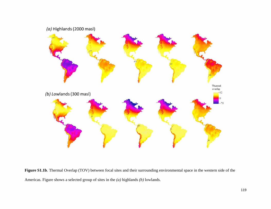
119

Figure S1.1b. Thermal Overlap (TOV) between focal sites and their surrounding environmental space in the western side of the

Americas. Figure shows a selected group of sites in the (a) highlands (b) lowlands.

120

Figure S1.2. Thermal overlap as a function of altitude: (a) This relationship is linear for most of

the Americas (three sites in eastern side), but is non-linear in some regions east of the Rockies in

North America between 33°N and 48°N (b).

121

Figure S1.3. Elevation at which thermal overlap decreases to zero at all locations across the

Americas.

122

Figure S1.4. Compositional similarity between pairwise comparisons of quadrats across a

latitudinal gradient in the Americas’ mountains. (a) Amphibians and (b) Mammals. Upper panel

shows pairwise comparisons of sites between sites in the highlands and lower panel in lowlands

123

Figure S1.5. Potential ‘passes’ in northern South America that could allow species to circumvent

thermal barriers imposed by differences in thermal regimes between focal sites. Arrows represent

potential dispersal routes.

124

APPENDICES CHAPTER 2

Table S2.1. Non-parametric correlations coefficients (Spearman rank, rs) between endemism for mammals and amphibians and

environmental predictors. Metrics of endemism based on species range size cut-offs (QE = first quartile; 50K = 50,000 km2 and 250K

= 250,000 km2), inverse range size (WE = Weighted Endemism) and median range size (Median). Results shown are for c. 110 km x

110 km spatial resolution.

Hypothesis/Predictors Amphibians Mammals

QE 50K 250K WE Median QE 50K 250K WE Median H1: Climate velocity -0.26 -0.42 -0.50 -0.39 0.43 -0.32 -0.40 -0.51 -0.56 0.43

H2: Climate seasonality

Mean temperature -0.26 -0.37 -0.44 -0.70 0.42 -0.27 -0.31 -0.42 -0.66 0.45

Total precipitation 0.001 0.02 0.02 0.02 -0.02 0.03 0.05 0.08 0.11 -0.16

H3: Climate distinctiveness (rarity)

Mean temperature 0.06 0.06 0.06 -0.17 -0.05 0.09 0.09 0.06 -0.09 -0.00003

Total precipitation 0.27 0.42 0.49 0.62 -0.34 0.29 0.34 0.41 0.63 -0.39

Precipitation seasonality 0.09 0.13 0.19 0.20 -0.28 0.11 0.19 0.27 0.27 -0.28

Temperature seasonality -0.14 -0.12 -0.14 -0.32 0.06 -0.10 -0.09 -0.10 -0.26 0.04

H4: Spatial heterogeneity

in climate:

Mean temperature 0.21 0.30 0.34 0.13 -0.24 0.25 0.30 0.33 0.27 -0.19

in topography:

Elevation 0.22 0.32 0.37 0.18 -0.29 0.27 0.32 0.37 0.32 -0.24

in habitat

Actual evapotranspiration 0.14 0.20 0.18 0.25 -0.14 0.18 0.21 0.23 0.32 -0.17

Potential evapotranspiration 0.23 0.39 0.48 0.37 -0.47 0.30 0.39 0.48 0.49 -0.43

H5: Total species richness 0.29 0.45 0.51 0.84 -0.40 0.29 0.32 0.37 0.74 -0.34

Other predictors

Productivity:

125

Potential evapotranspiration 0.06 0.11 0.17 0.41 -0.30 0.07 0.09 0.19 0.33 -0.33

Actual evapotranspiration 0.24 0.35 0.39 0.69 -0.26 0.22 0.23 0.26 0.58 -0.29

Precipitation total 0.26 0.39 0.41 0.66 -0.21 0.22 0.21 0.20 0.50 -0.18

Current - Mean temperature 0.11 0.18 0.24 0.49 -0.30 0.10 0.13 0.23 0.40 -0.32

Past mean temperature (LGM) 0.12 0.20 0.26 0.49 -0.30 0.12 0.16 0.28 0.45 -0.35

Area -0.11 -0.14 -0.18 -0.28 0.25 -0.10 -0.11 -0.15 -0.20 0.18

Glaciated areas (LGM) -0.05 -0.13 -0.19 -0.29 0.22 -0.07 -0.13 -0.23 -0.40 0.33

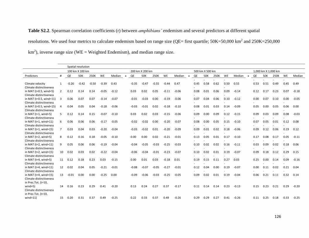
126

Table S2.2. Spearman correlation coefficients (r) between amphibians’ endemism and several predictors at different spatial

resolutions. We used four metrics to calculate endemism based on range size (QE= first quartile; 50K=50,000 km2 and 250K=250,000

km2), inverse range size (WE = Weighted Endemism), and median range size.

Spatial resolution

100 km X 100 km 200 km X 200 km 500 km X 500 km 1,000 km X 1,000 km

Predictors # QE 50K 250K WE Median x QE 50K 250K WE Median x QE 50K 250K WE Median x QE 50K 250K WE Median

Climate velocity 1 -0.26 -0.42 -0.50 -0.39 0.43 -0.35 -0.47 -0.55 -0.44 0.47

-0.45

-0.58

-0.62

-0.50 0.55

-0.53

-0.51

-0.49

-0.45 0.49

Climate distinctiveness in MAT (t=0.5, wind=5) 2 0.12 0.14 0.14 -0.05 -0.12 0.03 0.02 0.05 -0.11 -0.06

-0.08 0.01 0.06

-0.09 -0.14 0.12 0.17 0.23 0.07 -0.18

Climate distinctiveness in MAT (t=0.5, wind=11) 3 0.06 0.07 0.07 -0.14 -0.07 -0.01 -0.03 0.00 -0.19 -0.06

-0.07 0.04 0.06

-0.10 -0.12 0.00 0.07 0.10 0.00 -0.05

Climate distinctiveness in MAT (t=0.5, wind=15) 4 0.04 0.05 0.04 -0.18 -0.06 -0.03 -0.01 0.02 -0.18 -0.10

-0.08 0.01 0.03

-0.14 -0.09

-0.05 0.00 0.05

-0.06 0.00

Climate distinctiveness in MAT (t=1, wind=5) 5 0.12 0.14 0.15 -0.07 -0.10 0.03 0.02 0.03 -0.15 -0.06

-0.09 0.00 0.09

-0.12 -0.15 0.09 0.03 0.09

-0.08 -0.03

Climate distinctiveness in MAT (t=1, wind=11) 6 0.06 0.06 0.06 -0.17 -0.05 -0.02 -0.02 0.00 -0.20 -0.07

-0.08 0.00 0.05

-0.15 -0.10

-0.07

-0.05

-0.01

-0.12 0.08

Climate distinctiveness in MAT (t=1, wind=15) 7 0.03 0.04 0.03 -0.20 -0.04 -0.03 -0.02 0.01 -0.20 -0.09

-0.09

-0.01 0.02

-0.18 -0.06

-0.09

-0.12

-0.06

-0.19 0.12

Climate distinctiveness in MAT (t=2, wind=5) 8 0.12 0.16 0.18 -0.05 -0.10 0.00 0.00 0.02 -0.21 -0.01

-0.13

-0.05 0.01

-0.17 -0.10 0.17 0.08 0.17

-0.05 -0.11

Climate distinctiveness in MAT (t=2, wind=11) 9 0.05 0.06 0.06 -0.19 -0.04 -0.04 -0.05 -0.03 -0.25 -0.03

-0.10

-0.02 0.02

-0.16 -0.11

-0.03

-0.09

-0.02

-0.18 0.06

Climate distinctiveness in MAT (t=2, wind=15) 10 0.02 0.03 0.02 -0.22 -0.04 -0.06 -0.04 -0.01 -0.23 -0.07

-0.10

-0.02 0.01

-0.19 -0.07

-0.09

-0.18

-0.12

-0.29 0.15

Climate distinctiveness in MAT (t=4, wind=5) 11 0.12 0.18 0.23 0.03 -0.15 0.00 0.01 0.03 -0.18 0.01

-0.19

-0.15

-0.11

-0.27 0.03 0.25 0.00 0.14

-0.09 -0.16

Climate distinctiveness in MAT (t=4, wind=11) 12 0.02 0.04 0.05 -0.21 -0.01 -0.08 -0.07 -0.05 -0.27 -0.01

-0.12

-0.04 0.00

-0.19 -0.07 0.00

-0.11

-0.02

-0.21 0.04

Climate distinctiveness in MAT (t=4, wind=15) 13 -0.01 0.00 0.00 -0.25 0.00 -0.09 -0.06 -0.03 -0.25 -0.05

-0.09

-0.02 0.01

-0.19 -0.04

-0.06

-0.21

-0.11

-0.32 0.14

Climate distinctiveness in Prec.Tot. (t=10, wind=5) 14 0.16 0.23 0.29 0.41 -0.20 0.13 0.24 0.27 0.37 -0.17 0.11 0.14 0.14 0.23 -0.13 0.15 0.23 0.21 0.29 -0.20 Climate distinctiveness in Prec.Tot. (t=10, wind=11) 15 0.20 0.31 0.37 0.49 -0.25 0.22 0.33 0.37 0.49 -0.26 0.29 0.29 0.27 0.41 -0.26 0.11 0.25 0.18 0.33 -0.25

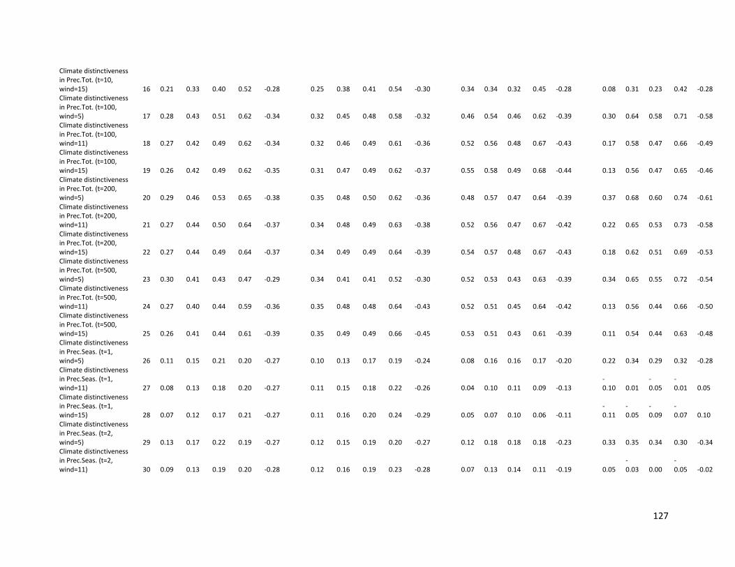
127

Climate distinctiveness in Prec.Tot. (t=10, wind=15) 16 0.21 0.33 0.40 0.52 -0.28 0.25 0.38 0.41 0.54 -0.30 0.34 0.34 0.32 0.45 -0.28 0.08 0.31 0.23 0.42 -0.28 Climate distinctiveness in Prec.Tot. (t=100, wind=5) 17 0.28 0.43 0.51 0.62 -0.34 0.32 0.45 0.48 0.58 -0.32 0.46 0.54 0.46 0.62 -0.39 0.30 0.64 0.58 0.71 -0.58 Climate distinctiveness in Prec.Tot. (t=100, wind=11) 18 0.27 0.42 0.49 0.62 -0.34 0.32 0.46 0.49 0.61 -0.36 0.52 0.56 0.48 0.67 -0.43 0.17 0.58 0.47 0.66 -0.49 Climate distinctiveness in Prec.Tot. (t=100, wind=15) 19 0.26 0.42 0.49 0.62 -0.35 0.31 0.47 0.49 0.62 -0.37 0.55 0.58 0.49 0.68 -0.44 0.13 0.56 0.47 0.65 -0.46 Climate distinctiveness in Prec.Tot. (t=200, wind=5) 20 0.29 0.46 0.53 0.65 -0.38 0.35 0.48 0.50 0.62 -0.36 0.48 0.57 0.47 0.64 -0.39 0.37 0.68 0.60 0.74 -0.61 Climate distinctiveness in Prec.Tot. (t=200, wind=11) 21 0.27 0.44 0.50 0.64 -0.37 0.34 0.48 0.49 0.63 -0.38 0.52 0.56 0.47 0.67 -0.42 0.22 0.65 0.53 0.73 -0.58 Climate distinctiveness in Prec.Tot. (t=200, wind=15) 22 0.27 0.44 0.49 0.64 -0.37 0.34 0.49 0.49 0.64 -0.39 0.54 0.57 0.48 0.67 -0.43 0.18 0.62 0.51 0.69 -0.53 Climate distinctiveness in Prec.Tot. (t=500, wind=5) 23 0.30 0.41 0.43 0.47 -0.29 0.34 0.41 0.41 0.52 -0.30 0.52 0.53 0.43 0.63 -0.39 0.34 0.65 0.55 0.72 -0.54 Climate distinctiveness in Prec.Tot. (t=500, wind=11) 24 0.27 0.40 0.44 0.59 -0.36 0.35 0.48 0.48 0.64 -0.43 0.52 0.51 0.45 0.64 -0.42 0.13 0.56 0.44 0.66 -0.50 Climate distinctiveness in Prec.Tot. (t=500, wind=15) 25 0.26 0.41 0.44 0.61 -0.39 0.35 0.49 0.49 0.66 -0.45 0.53 0.51 0.43 0.61 -0.39 0.11 0.54 0.44 0.63 -0.48 Climate distinctiveness in Prec.Seas. (t=1, wind=5) 26 0.11 0.15 0.21 0.20 -0.27 0.10 0.13 0.17 0.19 -0.24 0.08 0.16 0.16 0.17 -0.20 0.22 0.34 0.29 0.32 -0.28 Climate distinctiveness in Prec.Seas. (t=1, wind=11) 27 0.08 0.13 0.18 0.20 -0.27 0.11 0.15 0.18 0.22 -0.26 0.04 0.10 0.11 0.09 -0.13

-0.10 0.01

-0.05

-0.01 0.05

Climate distinctiveness in Prec.Seas. (t=1, wind=15) 28 0.07 0.12 0.17 0.21 -0.27 0.11 0.16 0.20 0.24 -0.29 0.05 0.07 0.10 0.06 -0.11

-0.11

-0.05

-0.09

-0.07 0.10

Climate distinctiveness in Prec.Seas. (t=2, wind=5) 29 0.13 0.17 0.22 0.19 -0.27 0.12 0.15 0.19 0.20 -0.27 0.12 0.18 0.18 0.18 -0.23 0.33 0.35 0.34 0.30 -0.34 Climate distinctiveness in Prec.Seas. (t=2, wind=11) 30 0.09 0.13 0.19 0.20 -0.28 0.12 0.16 0.19 0.23 -0.28 0.07 0.13 0.14 0.11 -0.19 0.05

-0.03 0.00

-0.05 -0.02

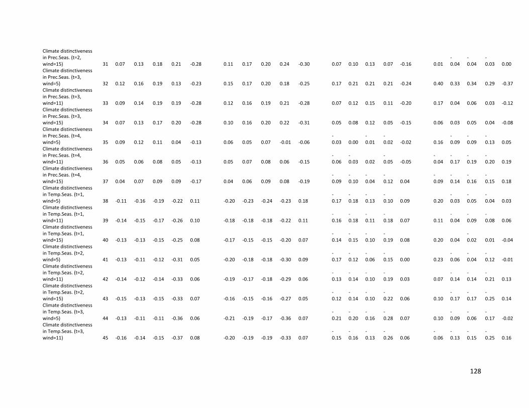
128

Climate distinctiveness in Prec.Seas. (t=2, wind=15) 31 0.07 0.13 0.18 0.21 -0.28 0.11 0.17 0.20 0.24 -0.30 0.07 0.10 0.13 0.07 -0.16 0.01

-0.04

-0.04

-0.03 0.00

Climate distinctiveness in Prec.Seas. (t=3, wind=5) 32 0.12 0.16 0.19 0.13 -0.23 0.15 0.17 0.20 0.18 -0.25 0.17 0.21 0.21 0.21 -0.24 0.40 0.33 0.34 0.29 -0.37 Climate distinctiveness in Prec.Seas. (t=3, wind=11) 33 0.09 0.14 0.19 0.19 -0.28 0.12 0.16 0.19 0.21 -0.28 0.07 0.12 0.15 0.11 -0.20 0.17 0.04 0.06 0.03 -0.12 Climate distinctiveness in Prec.Seas. (t=3, wind=15) 34 0.07 0.13 0.17 0.20 -0.28 0.10 0.16 0.20 0.22 -0.31 0.05 0.08 0.12 0.05 -0.15 0.06 0.03 0.05 0.04 -0.08 Climate distinctiveness in Prec.Seas. (t=4, wind=5) 35 0.09 0.12 0.11 0.04 -0.13 0.06 0.05 0.07 -0.01 -0.06

-0.03 0.00

-0.01

-0.02 -0.02 0.16

-0.09

-0.09

-0.13 0.05

Climate distinctiveness in Prec.Seas. (t=4, wind=11) 36 0.05 0.06 0.08 0.05 -0.13 0.05 0.07 0.08 0.06 -0.15

-0.06

-0.03 0.02

-0.05 -0.05

-0.04

-0.17

-0.19

-0.20 0.19

Climate distinctiveness in Prec.Seas. (t=4, wind=15) 37 0.04 0.07 0.09 0.09 -0.17 0.04 0.06 0.09 0.08 -0.19

-0.09

-0.10

-0.04

-0.12 0.04

-0.09

-0.14

-0.16

-0.15 0.18

Climate distinctiveness in Temp.Seas. (t=1, wind=5) 38 -0.11 -0.16 -0.19 -0.22 0.11 -0.20 -0.23 -0.24 -0.23 0.18

-0.17

-0.18

-0.13

-0.10 0.09 0.20

-0.03

-0.05

-0.04 0.03

Climate distinctiveness in Temp.Seas. (t=1, wind=11) 39 -0.14 -0.15 -0.17 -0.26 0.10 -0.18 -0.18 -0.18 -0.22 0.11

-0.16

-0.18

-0.11

-0.18 0.07 0.11

-0.04

-0.09

-0.08 0.06

Climate distinctiveness in Temp.Seas. (t=1, wind=15) 40 -0.13 -0.13 -0.15 -0.25 0.08 -0.17 -0.15 -0.15 -0.20 0.07

-0.14

-0.15

-0.10

-0.19 0.08 0.20 0.04

-0.02 0.01 -0.04

Climate distinctiveness in Temp.Seas. (t=2, wind=5) 41 -0.13 -0.11 -0.12 -0.31 0.05 -0.20 -0.18 -0.18 -0.30 0.09

-0.17

-0.12

-0.06

-0.15 0.00 0.23

-0.06

-0.04

-0.12 -0.01

Climate distinctiveness in Temp.Seas. (t=2, wind=11) 42 -0.14 -0.12 -0.14 -0.33 0.06 -0.19 -0.17 -0.18 -0.29 0.06

-0.13

-0.14

-0.10

-0.19 0.03 0.07

-0.14

-0.14

-0.21 0.13

Climate distinctiveness in Temp.Seas. (t=2, wind=15) 43 -0.15 -0.13 -0.15 -0.33 0.07 -0.16 -0.15 -0.16 -0.27 0.05

-0.12

-0.14

-0.10

-0.22 0.06 0.10

-0.17

-0.17

-0.25 0.14

Climate distinctiveness in Temp.Seas. (t=3, wind=5) 44 -0.13 -0.11 -0.11 -0.36 0.06 -0.21 -0.19 -0.17 -0.36 0.07

-0.21

-0.20

-0.16

-0.28 0.07 0.10

-0.09

-0.06

-0.17 -0.02

Climate distinctiveness in Temp.Seas. (t=3, wind=11) 45 -0.16 -0.14 -0.15 -0.37 0.08 -0.20 -0.19 -0.19 -0.33 0.07

-0.15

-0.16

-0.13

-0.26 0.06

-0.06

-0.13

-0.15

-0.25 0.16

129

Climate distinctiveness in Temp.Seas. (t=3, wind=15) 46 -0.16 -0.14 -0.17 -0.37 0.08 -0.18 -0.17 -0.17 -0.31 0.06

-0.14

-0.17

-0.15

-0.30 0.10

-0.17

-0.32

-0.30

-0.43 0.31

Climate distinctiveness in Temp.Seas. (t=4, wind=5) 47 -0.11 -0.11 -0.10 -0.36 0.10 -0.22 -0.22 -0.19 -0.40 0.10

-0.22

-0.22

-0.18

-0.31 0.09 0.04

-0.10

-0.07

-0.15 -0.01

Climate distinctiveness in Temp.Seas. (t=4, wind=11) 48 -0.17 -0.16 -0.17 -0.41 0.09 -0.21 -0.22 -0.22 -0.38 0.09

-0.15

-0.17

-0.14

-0.27 0.07

-0.10

-0.22

-0.22

-0.30 0.23

Climate distinctiveness in Temp.Seas. (t=4, wind=15) 49 -0.17 -0.16 -0.18 -0.40 0.10 -0.19 -0.19 -0.20 -0.35 0.08

-0.14

-0.16

-0.14

-0.29 0.10

-0.15

-0.37

-0.32

-0.45 0.35

Habitat heterogeneity (Range) in AET 50 0.14 0.19 0.18 0.24 -0.14 0.17 0.23 0.26 0.36 -0.29 0.20 0.31 0.38 0.39 -0.43 0.47 0.45 0.43 0.48 -0.48 Habitat heterogeneity (Range) in PET 51 0.24 0.41 0.50 0.39 -0.48 0.33 0.46 0.56 0.45 -0.54 0.37 0.56 0.64 0.51 -0.62 0.66 0.67 0.69 0.60 -0.70 Habitat heterogeneity (Range) in MAT 52 0.22 0.32 0.36 0.16 -0.26 0.28 0.33 0.38 0.19 -0.29 0.21 0.31 0.38 0.17 -0.32 0.33 0.22 0.27 0.08 -0.24 Habitat heterogeneity (Range) in Altitude 53 0.22 0.33 0.38 0.19 -0.29 0.29 0.36 0.42 0.25 -0.34 0.30 0.41 0.49 0.32 -0.43 0.52 0.47 0.50 0.35 -0.47 Habitat heterogeneity (Sd) in AET 54 0.14 0.20 0.18 0.25 -0.14 0.20 0.27 0.27 0.35 -0.25 0.29 0.40 0.39 0.46 -0.35 0.41 0.55 0.45 0.61 -0.50 Habitat heterogeneity (Sd) in PET 55 0.23 0.39 0.48 0.37 -0.47 0.31 0.43 0.53 0.41 -0.52 0.31 0.48 0.56 0.40 -0.56 0.47 0.41 0.48 0.36 -0.53 Habitat heterogeneity (Sd) in MAT 56 0.21 0.30 0.34 0.13 -0.24 0.26 0.30 0.35 0.15 -0.26 0.11 0.20 0.27 0.04 -0.23 0.11

-0.04 0.03

-0.14 -0.06

Habitat heterogeneity (Sd) in Altitude 57 0.22 0.32 0.37 0.18 -0.29 0.28 0.35 0.41 0.23 -0.34 0.28 0.41 0.48 0.30 -0.44 0.53 0.44 0.46 0.32 -0.47

Seasonality in MAT 58 -0.26 -0.37 -0.44 -0.70 0.42 -0.36 -0.44 -0.48 -0.70 0.43

-0.54

-0.55

-0.50

-0.71 0.44

-0.34

-0.67

-0.56

-0.77 0.57

Seasonality in Prec. Tot. 59 0.00 0.02 0.02 0.02 -0.02 0.03 0.02 0.01 0.03 -0.04 0.05 0.07 0.05 0.08 -0.07 0.32 0.16 0.09 0.16 -0.15 Climate relict in MAT (wind=5) 60 0.09 0.08 0.07 0.02 -0.04 0.12 0.09 0.11 0.02 -0.06 0.08 0.03 0.00

-0.07 0.05

-0.20

-0.23

-0.29

-0.24 0.22

Climate relict in MAT (wind=11) 61 0.12 0.10 0.11 0.00 -0.04 0.15 0.08 0.08 -0.04 0.00

-0.09

-0.13

-0.14

-0.23 0.17

-0.23

-0.25

-0.30

-0.29 0.28

Climate relict in MAT (wind=15) 62 0.13 0.10 0.11 -0.01 -0.02 0.13 0.04 0.04 -0.09 0.03

-0.14

-0.16

-0.16

-0.27 0.19

-0.24

-0.25

-0.28

-0.29 0.28

Productivity in PET 63 0.06 0.11 0.17 0.41 -0.30 0.11 0.17 0.19 0.40 -0.29 0.21 0.24 0.24 0.38 -0.27 0.38 0.43 0.36 0.51 -0.41

Productivity in AET 64 0.24 0.35 0.39 0.69 -0.26 0.32 0.42 0.42 0.69 -0.27 0.53 0.53 0.43 0.72 -0.31 0.07 0.64 0.55 0.74 -0.44

Area 65 -0.12 -0.14 -0.18 -0.28 0.25 -0.13 -0.16 -0.19 -0.28 0.24

-0.19

-0.20

-0.19

-0.28 0.24 0.04

-0.21

-0.27

-0.31 0.28

Glaciated areas 66 -0.05 -0.13 -0.19 -0.29 0.22 -0.06 -0.16 -0.20 -0.28 0.24

-0.17

-0.24

-0.25

-0.29 0.25

-0.41

-0.28

-0.26

-0.29 0.28

MAT 67 0.11 0.18 0.24 0.49 -0.30 0.17 0.24 0.26 0.49 -0.30 0.30 0.31 0.30 0.47 -0.30 0.34 0.52 0.43 0.60 -0.47

MAT-Past 68 0.12 0.20 0.26 0.49 -0.30 0.19 0.26 0.29 0.49 -0.31 0.32 0.34 0.32 0.48 -0.31 0.38 0.54 0.45 0.60 -0.47

Precipitation total 69 0.26 0.39 0.40 0.66 -0.21 0.34 0.44 0.42 0.65 -0.22 0.54 0.52 0.40 0.66 -0.27 0.01 0.61 0.50 0.69 -0.42

130

Altitude 70 0.10 0.13 0.17 0.06 -0.19 0.13 0.15 0.21 0.11 -0.24 0.15 0.24 0.30 0.18 -0.32 0.47 0.28 0.32 0.22 -0.35

Richness 71 0.29 0.45 0.51 0.85 -0.40 0.41 0.54 0.56 0.85 -0.43 0.65 0.70 0.63 0.88 -0.52 0.32 0.83 0.76 0.93 -0.70

131

Table S2.3. Spearman correlation coefficients (r) between mammals’ endemism and several predictors at different spatial resolutions.

We used five metrics to calculate endemism based on range size (QE= first quartile; 50K=50,000 km2 and 250K=250,000 km2),

inverse range size (WE = Weighted Endemism) and median range size (Median).

Spatial resolution

100 km X 100 km 200 km X 200 km 500 km X 500 km 1,000 km X 1,000 km

Predictors # QE 50K 250K WE Median QE 50K 250K WE Median QE 50K 250K WE Median QE 50K 250K WE Median

Climate velocity 1 -0.32 -0.40 -0.51 -0.55 0.43 -0.41 -0.47 -0.55 -0.59 0.45

-0.54

-0.57

-0.63

-0.62 0.49

-0.57

-0.52

-0.55

-0.58 0.48

Climate distinctiveness in MAT (t=0.5, wind=5) 2 0.14 0.16 0.15 0.05 -0.07 0.07 0.08 0.07 -0.02 -0.05 0.08 0.06 0.09 0.00 -0.12 0.19 0.10 0.10 0.06 -0.13 Climate distinctiveness in MAT (t=0.5, wind=11) 3 0.09 0.10 0.07 -0.07 -0.02 0.02 0.01 0.00 -0.14 -0.01 0.06 0.06 0.05

-0.04 -0.08 0.08

-0.03

-0.02

-0.01 0.01

Climate distinctiveness in MAT (t=0.5, wind=15) 4 0.07 0.07 0.03 -0.12 0.00 0.01 0.02 0.01 -0.14 -0.03 0.02 0.04 0.02

-0.07 -0.03 0.02

-0.10

-0.08

-0.10 0.05

Climate distinctiveness in MAT (t=1, wind=5) 5 0.15 0.16 0.15 0.03 -0.04 0.07 0.06 0.04 -0.07 -0.02 0.07 0.08 0.08

-0.02 -0.09 0.07 0.01 0.00

-0.06 -0.06

Climate distinctiveness in MAT (t=1, wind=11) 6 0.09 0.09 0.06 -0.09 0.00 0.03 0.02 -0.01 -0.15 -0.01 0.01 0.03 0.01

-0.08 -0.03

-0.05

-0.12

-0.12

-0.12 0.11

Climate distinctiveness in MAT (t=1, wind=15) 7 0.07 0.06 0.03 -0.14 0.01 0.02 0.02 0.00 -0.16 -0.02 0.00 0.02

-0.01

-0.11 0.01

-0.08

-0.18

-0.16

-0.20 0.14

Climate distinctiveness in MAT (t=2, wind=5) 8 0.16 0.19 0.20 0.08 -0.06 0.06 0.05 0.03 -0.12 0.04

-0.02

-0.01

-0.01

-0.11 -0.03 0.15 0.02 0.02

-0.03 -0.07

Climate distinctiveness in MAT (t=2, wind=11) 9 0.09 0.09 0.07 -0.10 0.00 0.00 -0.01 -0.03 -0.20 0.04

-0.01 0.00

-0.01

-0.11 -0.04

-0.04

-0.13

-0.13

-0.15 0.16

Climate distinctiveness in MAT (t=2, wind=15) 10 0.06 0.06 0.02 -0.15 0.02 -0.01 -0.01 -0.02 -0.19 0.01

-0.02 0.01

-0.02

-0.14 -0.01

-0.12

-0.22

-0.22

-0.26 0.24

Climate distinctiveness in MAT (t=4, wind=5) 11 0.18 0.23 0.28 0.18 -0.14 0.06 0.07 0.07 -0.07 0.03

-0.12

-0.14

-0.14

-0.24 0.11 0.19 0.02 0.03

-0.02 -0.06

132

Climate distinctiveness in MAT (t=4, wind=11) 12 0.07 0.08 0.06 -0.11 0.04 -0.03 -0.04 -0.05 -0.22 0.05

-0.05

-0.04

-0.05

-0.17 0.03

-0.01

-0.14

-0.14

-0.18 0.16

Climate distinctiveness in MAT (t=4, wind=15) 13 0.03 0.04 0.00 -0.18 0.06 -0.04 -0.04 -0.05 -0.22 0.02

-0.04

-0.01

-0.03

-0.16 0.03

-0.11

-0.23

-0.22

-0.29 0.23

Climate distinctiveness in Prec.Tot. (t=10, wind=5) 14 0.19 0.24 0.29 0.49 -0.28 0.17 0.22 0.25 0.42 -0.27 0.18 0.17 0.18 0.31 -0.22 0.20 0.05 0.09 0.22 -0.14 Climate distinctiveness in Prec.Tot. (t=10, wind=11) 15 0.23 0.28 0.34 0.54 -0.33 0.23 0.27 0.32 0.50 -0.33 0.29 0.25 0.23 0.41 -0.28 0.22 0.11 0.10 0.25 -0.10 Climate distinctiveness in Prec.Tot. (t=10, wind=15) 16 0.24 0.29 0.35 0.56 -0.34 0.26 0.30 0.33 0.52 -0.36 0.29 0.26 0.26 0.42 -0.28 0.24 0.17 0.15 0.29 -0.18 Climate distinctiveness in Prec.Tot. (t=100, wind=5) 17 0.31 0.37 0.44 0.65 -0.37 0.33 0.37 0.41 0.58 -0.37 0.41 0.38 0.39 0.53 -0.44 0.54 0.46 0.44 0.54 -0.56 Climate distinctiveness in Prec.Tot. (t=100, wind=11) 18 0.30 0.35 0.42 0.63 -0.38 0.33 0.36 0.40 0.58 -0.40 0.43 0.39 0.38 0.56 -0.44 0.44 0.38 0.36 0.47 -0.43 Climate distinctiveness in Prec.Tot. (t=100, wind=15) 19 0.29 0.34 0.41 0.63 -0.39 0.32 0.35 0.39 0.58 -0.41 0.43 0.39 0.37 0.55 -0.40 0.41 0.39 0.36 0.40 -0.38 Climate distinctiveness in Prec.Tot. (t=200, wind=5) 20 0.33 0.40 0.47 0.68 -0.40 0.35 0.39 0.43 0.61 -0.40 0.40 0.38 0.38 0.52 -0.43 0.62 0.59 0.55 0.62 -0.61 Climate distinctiveness in Prec.Tot. (t=200, wind=11) 21 0.30 0.36 0.44 0.66 -0.42 0.33 0.36 0.40 0.59 -0.43 0.40 0.38 0.35 0.53 -0.40 0.54 0.49 0.47 0.54 -0.50 Climate distinctiveness in Prec.Tot. (t=200, wind=15) 22 0.29 0.35 0.42 0.64 -0.42 0.32 0.35 0.39 0.58 -0.44 0.41 0.38 0.34 0.51 -0.37 0.49 0.48 0.45 0.48 -0.47 Climate distinctiveness in Prec.Tot. (t=500, wind=5) 23 0.29 0.34 0.39 0.49 -0.28 0.31 0.34 0.39 0.52 -0.35 0.39 0.40 0.41 0.53 -0.47 0.54 0.55 0.50 0.60 -0.55

133

Climate distinctiveness in Prec.Tot. (t=500, wind=11) 24 0.30 0.34 0.44 0.63 -0.44 0.32 0.37 0.43 0.60 -0.50 0.37 0.38 0.37 0.52 -0.43 0.44 0.41 0.39 0.47 -0.47 Climate distinctiveness in Prec.Tot. (t=500, wind=15) 25 0.28 0.34 0.43 0.64 -0.48 0.32 0.36 0.42 0.59 -0.50 0.36 0.35 0.32 0.48 -0.35 0.42 0.41 0.40 0.40 -0.45 Climate distinctiveness in Prec.Seas. (t=1, wind=5) 26 0.14 0.21 0.28 0.25 -0.23 0.15 0.20 0.25 0.25 -0.25 0.16 0.19 0.23 0.25 -0.29 0.31 0.19 0.20 0.35 -0.18 Climate distinctiveness in Prec.Seas. (t=1, wind=11) 27 0.12 0.19 0.26 0.25 -0.26 0.13 0.19 0.26 0.27 -0.30 0.09 0.15 0.15 0.18 -0.19

-0.04

-0.11

-0.11 0.00 0.16

Climate distinctiveness in Prec.Seas. (t=1, wind=15) 28 0.10 0.18 0.25 0.26 -0.27 0.14 0.20 0.27 0.28 -0.33 0.07 0.14 0.13 0.14 -0.13

-0.10

-0.14

-0.15

-0.05 0.18

Climate distinctiveness in Prec.Seas. (t=2, wind=5) 29 0.15 0.23 0.30 0.25 -0.23 0.15 0.22 0.28 0.27 -0.27 0.20 0.22 0.23 0.25 -0.32 0.38 0.31 0.31 0.41 -0.27 Climate distinctiveness in Prec.Seas. (t=2, wind=11) 30 0.12 0.20 0.28 0.26 -0.28 0.14 0.19 0.28 0.28 -0.32 0.12 0.20 0.18 0.20 -0.25 0.05 0.01

-0.01 0.08 0.04

Climate distinctiveness in Prec.Seas. (t=2, wind=15) 31 0.11 0.19 0.27 0.27 -0.29 0.13 0.19 0.27 0.28 -0.34 0.10 0.18 0.16 0.16 -0.20 0.02

-0.03

-0.05 0.06 0.04

Climate distinctiveness in Prec.Seas. (t=3, wind=5) 32 0.13 0.21 0.26 0.19 -0.17 0.14 0.23 0.29 0.26 -0.25 0.20 0.25 0.26 0.28 -0.36 0.41 0.43 0.40 0.40 -0.40 Climate distinctiveness in Prec.Seas. (t=3, wind=11) 33 0.12 0.20 0.28 0.26 -0.28 0.12 0.19 0.28 0.27 -0.33 0.10 0.18 0.20 0.19 -0.28 0.12 0.14 0.10 0.16 -0.11 Climate distinctiveness in Prec.Seas. (t=3, wind=15) 34 0.11 0.18 0.27 0.26 -0.30 0.12 0.19 0.28 0.26 -0.35 0.07 0.17 0.17 0.14 -0.20 0.06 0.07 0.05 0.12 -0.05 Climate distinctiveness in 35 0.07 0.08 0.11 0.00 0.00 0.05 0.09 0.12 0.03 -0.01 0.03 0.10 0.12 0.07 -0.17 0.00 0.08 0.05 0.00 -0.08

134

Prec.Seas. (t=4, wind=5) Climate distinctiveness in Prec.Seas. (t=4, wind=11) 36 0.06 0.11 0.16 0.09 -0.10 0.05 0.11 0.19 0.14 -0.22 0.00 0.10 0.12 0.06 -0.17

-0.17

-0.07

-0.12

-0.10 0.13

Climate distinctiveness in Prec.Seas. (t=4, wind=15) 37 0.05 0.11 0.18 0.14 -0.19 0.06 0.12 0.21 0.16 -0.27

-0.04 0.04 0.03

-0.02 -0.06

-0.17

-0.07

-0.13

-0.12 0.13

Climate distinctiveness in Temp.Seas. (t=1, wind=5) 38 -0.10 -0.12 -0.16 -0.17 0.02 -0.16 -0.18 -0.23 -0.18 0.06

-0.10

-0.13

-0.14 0.00 0.00 0.01 0.01 0.00 0.06 0.02

Climate distinctiveness in Temp.Seas. (t=1, wind=11) 39 -0.11 -0.11 -0.15 -0.21 0.04 -0.14 -0.14 -0.16 -0.15 0.02

-0.12

-0.08

-0.11

-0.07 0.07

-0.06

-0.01

-0.05 0.05 0.13

Climate distinctiveness in Temp.Seas. (t=1, wind=15) 40 -0.10 -0.10 -0.14 -0.21 0.03 -0.13 -0.11 -0.13 -0.14 0.00

-0.15

-0.11

-0.12

-0.11 0.11 0.03 0.10 0.05 0.19 -0.01

Climate distinctiveness in Temp.Seas. (t=2, wind=5) 41 -0.08 -0.07 -0.08 -0.24 0.04 -0.13 -0.13 -0.14 -0.24 0.05

-0.04

-0.07

-0.10

-0.06 -0.02 0.07 0.07 0.00 0.05 0.00

Climate distinctiveness in Temp.Seas. (t=2, wind=11) 42 -0.10 -0.09 -0.10 -0.26 0.04 -0.12 -0.11 -0.11 -0.21 0.01

-0.08

-0.08

-0.12

-0.11 0.03

-0.09

-0.04

-0.12

-0.02 0.15

Climate distinctiveness in Temp.Seas. (t=2, wind=15) 43 -0.10 -0.09 -0.11 -0.27 0.04 -0.11 -0.10 -0.10 -0.20 0.00

-0.12

-0.11

-0.14

-0.15 0.09

-0.06

-0.03

-0.10

-0.01 0.13

Climate distinctiveness in Temp.Seas. (t=3, wind=5) 44 -0.07 -0.05 -0.03 -0.24 0.06 -0.14 -0.11 -0.09 -0.27 0.05

-0.16

-0.15

-0.19

-0.19 0.05 0.02

-0.07

-0.08

-0.09 0.04

Climate distinctiveness in Temp.Seas. (t=3, wind=11) 45 -0.11 -0.09 -0.09 -0.29 0.06 -0.14 -0.11 -0.10 -0.24 0.02

-0.15

-0.14

-0.16

-0.19 0.05

-0.16

-0.17

-0.19

-0.13 0.23

Climate distinctiveness in Temp.Seas. (t=3, wind=15) 46 -0.11 -0.09 -0.11 -0.29 0.06 -0.12 -0.10 -0.09 -0.22 0.01

-0.14

-0.14

-0.17

-0.21 0.10

-0.29

-0.36

-0.36

-0.33 0.39

135

Climate distinctiveness in Temp.Seas. (t=4, wind=5) 47 -0.06 -0.03 0.00 -0.21 0.10 -0.15 -0.12 -0.10 -0.29 0.09

-0.18

-0.18

-0.21

-0.23 0.08

-0.03

-0.12

-0.15

-0.08 0.03

Climate distinctiveness in Temp.Seas. (t=4, wind=11) 48 -0.12 -0.10 -0.10 -0.32 0.08 -0.16 -0.13 -0.12 -0.28 0.05

-0.16

-0.15

-0.17

-0.20 0.07

-0.21

-0.27

-0.31

-0.24 0.25

Climate distinctiveness in Temp.Seas. (t=4, wind=15) 49 -0.12 -0.10 -0.12 -0.32 0.07 -0.14 -0.13 -0.12 -0.26 0.03

-0.16

-0.15

-0.18

-0.22 0.10

-0.31

-0.40

-0.43

-0.39 0.37

Habitat heterogeneity (Range) in AET 50 0.17 0.20 0.24 0.33 -0.18 0.22 0.26 0.33 0.41 -0.34 0.34 0.40 0.49 0.45 -0.52 0.50 0.59 0.60 0.55 -0.62 Habitat heterogeneity (Range) in PET 51 0.31 0.40 0.49 0.52 -0.45 0.40 0.49 0.55 0.57 -0.50 0.53 0.58 0.64 0.60 -0.56 0.72 0.68 0.71 0.69 -0.66 Habitat heterogeneity (Range) in MAT 52 0.26 0.31 0.35 0.30 -0.21 0.31 0.36 0.37 0.33 -0.22 0.34 0.34 0.39 0.30 -0.21 0.29 0.21 0.27 0.19 -0.15 Habitat heterogeneity (Range) in Altitude 53 0.27 0.32 0.37 0.34 -0.25 0.33 0.38 0.42 0.39 -0.29 0.42 0.44 0.50 0.44 -0.34 0.51 0.47 0.54 0.51 -0.43 Habitat heterogeneity (Sd) in AET 54 0.18 0.21 0.23 0.32 -0.17 0.24 0.28 0.30 0.39 -0.29 0.38 0.40 0.44 0.48 -0.45 0.54 0.55 0.58 0.59 -0.58 Habitat heterogeneity (Sd) in PET 55 0.30 0.39 0.48 0.49 -0.43 0.38 0.47 0.53 0.52 -0.47 0.46 0.51 0.57 0.48 -0.50 0.52 0.44 0.47 0.36 -0.44 Habitat heterogeneity (Sd) in MAT 56 0.25 0.30 0.33 0.27 -0.19 0.29 0.32 0.34 0.27 -0.19 0.23 0.21 0.27 0.15 -0.12 0.08

-0.07

-0.02

-0.09 0.07

Habitat heterogeneity (Sd) in Altitude 57 0.26 0.32 0.37 0.32 -0.24 0.32 0.37 0.41 0.37 -0.28 0.40 0.42 0.49 0.43 -0.34 0.53 0.44 0.50 0.48 -0.42

Seasonality in MAT 58 -0.27 -0.31 -0.42 -0.65 0.45 -0.33 -0.37 -0.44 -0.64 0.46

-0.44

-0.47

-0.48

-0.61 0.48

-0.57

-0.64

-0.63

-0.64 0.62

Seasonality in Prec. Tot. 59 0.03 0.05 0.08 0.11 -0.16 0.03 0.08 0.11 0.14 -0.16 0.09 0.14 0.11 0.20 -0.17 0.16 0.28 0.22 0.32 -0.24 Climate relict in MAT (wind=5) 60 0.09 0.09 0.07 0.04 0.00 0.13 0.13 0.09 0.05 0.01 0.04 0.00

-0.05

-0.09 0.12

-0.29

-0.31

-0.33

-0.31 0.34

Climate relict in MAT (wind=11) 61 0.12 0.12 0.08 0.03 0.02 0.13 0.10 0.02 -0.03 0.08

-0.02

-0.07

-0.11

-0.19 0.20

-0.30

-0.32

-0.33

-0.35 0.39

Climate relict in MAT (wind=15) 62 0.12 0.12 0.06 0.00 0.05 0.10 0.07 -0.02 -0.09 0.13

-0.04

-0.08

-0.12

-0.20 0.20

-0.30

-0.31

-0.32

-0.34 0.38

Productivity in PET 63 0.07 0.09 0.19 0.33 -0.32 0.10 0.14 0.23 0.33 -0.33 0.18 0.24 0.28 0.34 -0.36 0.42 0.53 0.50 0.52 -0.54

136

Productivity in AET 64 0.22 0.23 0.26 0.58 -0.29 0.27 0.26 0.25 0.55 -0.29 0.39 0.30 0.27 0.52 -0.32 0.46 0.39 0.38 0.49 -0.45

Area 65 -0.10 -0.11 -0.15 -0.20 0.17 -0.12 -0.11 -0.16 -0.17 0.19

-0.15

-0.12

-0.18

-0.10 0.23

-0.24

-0.16

-0.22

-0.06 0.28

Glaciated areas 66 -0.07 -0.13 -0.22 -0.35 0.33 -0.10 -0.17 -0.25 -0.36 0.34

-0.22

-0.27

-0.29

-0.38 0.36

-0.32

-0.39

-0.36

-0.43 0.43

MAT 67 0.10 0.13 0.23 0.40 -0.32 0.13 0.18 0.26 0.39 -0.33 0.23 0.28 0.30 0.39 -0.35 0.46 0.55 0.52 0.54 -0.54

MAT-Past 68 0.12 0.16 0.28 0.45 -0.35 0.17 0.22 0.31 0.45 -0.36 0.27 0.32 0.36 0.45 -0.39 0.48 0.58 0.57 0.58 -0.56

Precipitation total 69 0.22 0.21 0.20 0.50 -0.17 0.27 0.23 0.19 0.46 -0.18 0.36 0.26 0.20 0.44 -0.20 0.42 0.32 0.31 0.41 -0.34

Altitude 70 0.13 0.16 0.19 0.22 -0.28 0.16 0.20 0.24 0.26 -0.29 0.24 0.25 0.30 0.31 -0.31 0.39 0.32 0.35 0.44 -0.39

Richness 71 0.29 0.32 0.37 0.74 -0.34 0.37 0.39 0.40 0.74 -0.38 0.55 0.50 0.49 0.75 -0.48 0.68 0.63 0.66 0.76 -0.68

137

Table S2.4. Poisson, Hurdle and Zero-Inflated Poisson (ZIP) models form amphibians and mammals’ endemism.

Amphibians Models

Mammals Models Estimate

(Standard error)

Poisson Hurdle-Poisson ZIP Poisson Hurdle-Poisson ZIP

Climate stability

Df 2 4 4 2 4 4

AIC 8511 6018 6135 11691 10016 10014

Zeros obs. ₤

9558 9882 9863 9558 9224 9214

Climate seasonality

Df 2 4 4

AIC 8503 5993 5971 12236 10273 10246

Zeros obs. ₤

9283 9882 9883 8549 9224 9227

Climate distinctiveness

Df 2 4 4 2 4 4

AIC 8428 6012 6016 11724 10042 10054

Zeros obs. ₤

9282 9882 9882 8576 9224 9222

Climate heterogeneity

Df 2 4 4 2 4 4

AIC 8801 6177 6162 11996 10128 10110

Zeros obs. ₤ 9348 9882 9883 8641 9224 9227

Log L = maximized log-likelihood

AIC = Akaike Information Criterion

₤ Total Zero obs. for amphibians = 9882; Non-zeros obs.=564; Total obs. 10446

Total Zero obs. for mammals = 9224; Non-zeros obs.= 1222; Total obs. 10446

138

Figure S2.1. Broad scale patterns of amphibian endemism using five metrics and four spatial resolutions. Metrics were constructed

using range size cut-offs (first quartile, 50K km2 and 250K km2 ), inverse range size (Weighted Endemism, WE) and median range

size.

139

Figure S2.2. Broad scale patterns of mammal endemism using five metrics and four spatial resolutions. Metrics were constructed

using range size cut-offs (first quartile, 50K km2 and 250K km2) and inverse range size (Weighted Endemism, WE), and median range

size.

140

Figure S2.3. Spatial congruence between mammals and amphibians using various metrics of

endemism a) Inverse range size, b) Median range size, c) Range size threshold (smallest

quartile), and d) Range size threshold (<50,000 Km2).

141

Figure S2.4a. Number of endemic species (boxplots) in mountain systems (300 to 2,500 meters

above the sea level) along a latitudinal gradient (greyscale bands represent approximately 10

degrees) for a) amphibians and b) mammals.

142

Figure S4b. Number of range-restricted species in mountains (>300 meters above sea level,

m.a.s.l) and low elevations (< 300m).

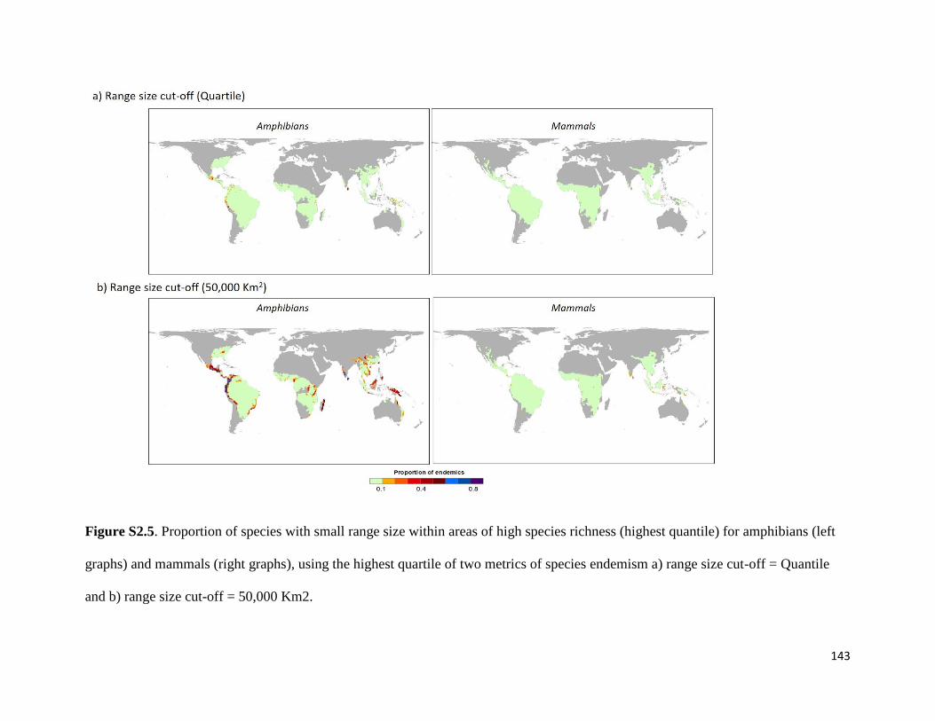
143

Figure S2.5. Proportion of species with small range size within areas of high species richness (highest quantile) for amphibians (left

graphs) and mammals (right graphs), using the highest quartile of two metrics of species endemism a) range size cut-off = Quantile

and b) range size cut-off = 50,000 Km2.

144

Figure S2.6. Spearman’s rank correlation coefficient (r, dotted line indicates r = 0.5) among

metrics of species endemism and total species richness. Metrics were constructed using range

size cut-offs (first quartile, ranges smaller than 5x104 km2, and ranges smaller than 2.5x105 km2),

inverse range size (Weighted Endemism, WE) and median range size.

145

Figure S2.7. Coefficient of determination (grey bars, R2) and collinearity (red lines, Variance

Inflation Factor, VIF) between amphibians’ endemism as a function of climate velocity (CV)

plus each other predictor, using two metrics of endemism a) Weighted endemism (WE), and b)

Median range size. Red dashed line represents VIF = 2.5 (above this line is high concern

regarding collinearity between variables). MAT = Mean annual temperature, AET = Actual

evapotranspiration, PET = Potential evapotranspiration, Prec. = Total precipitation.

146

Figure S2.8. Coefficient of determination (grey bars, R2) and collinearity (red lines, Variance

Inflation Factor, VIF) between mammals’ endemism as a function of climate velocity (CV) plus

each other predictor, using two metrics of endemism a) Weighted endemism (WE), and b)

Median range size. Red dashed line represents VIF = 2.5 (above this line is high concern

regarding collinearity between variables). MAT = Mean annual temperature, AET = Actual

evapotranspiration, PET = Potential evapotranspiration, Prec. = Total precipitation.

147

Figure S2.9. Models predicting endemism (using Median range size) for a) Climate velocity and

b) Spatial heterogeneity. (i) Variance partitioning (variance contribution of each predictor and

shared variance) and (ii) path analysis (the darker the line the stronger the effect on that

relationship);. AET = Actual evapotranspiration; CV = Climate velocity; SH-PET = Spatial

heterogeneity in potential evapotranspiration; PET = potential evapotranspiration; Richness =

Total species richness.

.

148

Figure S2.10. Models predicting endemism (using Weighted Endemism, WE) for a) Climate

velocity and b) Spatial heterogeneity. (i) Variance partitioning (variance contribution of each

predictor and shared variance) and (ii) path analysis (the darker the line the stronger the effect on

that relationship);. AET = Actual evapotranspiration; CV = Climate velocity; SH-PET = Spatial

heterogeneity in potential evapotranspiration; PET = potential evapotranspiration; Richness =

Total species richness.

149

Figure S2.11. Total species richness as a function of endemism a) Weighted endemism (WE)

and b) Median range size for amphibians and mammals. Variance explained is shown (R2).

150

Figure S2.12. Cross-continental validation from best Ordinary least squares (OLS) and spatial

autoregressive (SAR) models predicting broad scale patterns of endemism for amphibians and

mammals, using two metrics of endemism a) Median range size and b) Weighted endemism. SH-

PET = Spatial heterogeneity in potential evapotranspiration; PET = potential evapotranspiration;

CD-PT = Climate distinctiveness in Total precipitation; and, Richness = Total species richness.

151

Figure S2.13. Cross-continental validation from best Ordinary least squares (OLS) and spatial

autoregressive (SAR) models predicting broad scale patterns of endemism for amphibians and

mammals, using two metrics of endemism a) Median range size and b) Weighted endemism.

SH_PET = Spatial heterogeneity in potential evapotranspiration; PET = potential

152

evapotranspiration; CD_PT = Climate distinctiveness in Total precipitation; and, Richness =

Total species richness. Here we used some continental masses instead of realms to demonstrate

that models failed to predict endemism in various geographic settings.

153

Figure S2.14. Hanging rotograms from hurdle models (amphibians and mammals) for past climate (top graphs) and current climate

(bottom graphs).

154

Figure S2.15. Predicted vs. observed endemic species (amphibians and mammals) from hurdle

models for a) climate velocity; and b) Spatial heterogeneity in potential evapotranspiration.