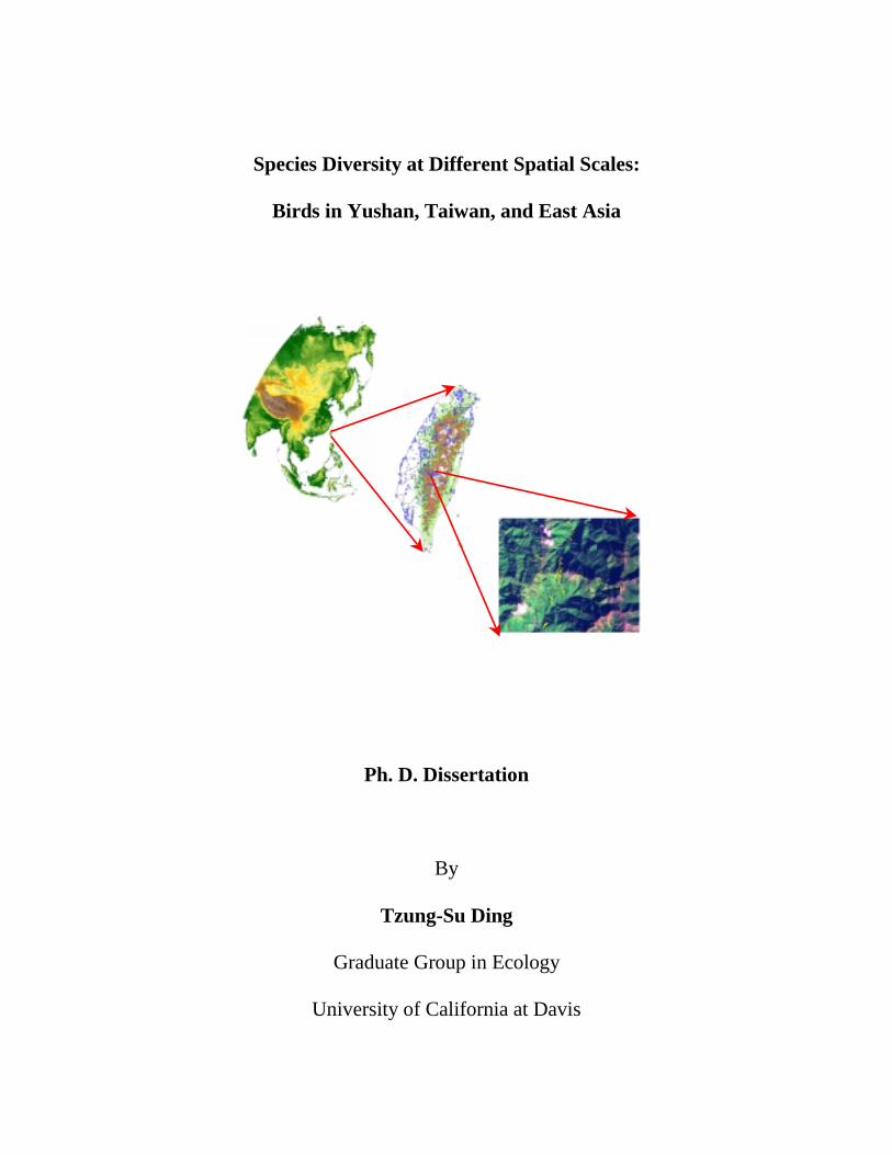
Species Diversity at Different Spatial Scales:

Birds in Yushan, Taiwan, and East Asia

Ph. D. Dissertation

By

Tzung-Su Ding

Graduate Group in Ecology

University of California at Davis

ii

iii

Acknowledgements

This dissertation is dedicated to my parents, brothers, and sisters. It is simple.

My education would not go this far without their support and loves.

Shu Geng, my major professor, deserves my greatest gratitude. His exceptional

guidance, support, friendship, and enthusiasm are critical for my studies in Davis and will

inspire me in my entire career.

The financial support from Ministry of Education, Republic of China, makes my

studies in Davis possible. My sincere gratitude is due to all the taxpayers in Taiwan.

The grant from the Pacific Rim Research Program at University of California supported

my study on the avifauna of East Asia and several invaluable field trips.

Art Shapiro and Susan Ustin made great advice to improve this dissertation.

Pei-Fen Lee, my long-time mentor, provided tremendous support and help for my studies.

Fu-Shiung Hsu helped me locate essential data for the study on Taiwan’s avifauna.

Minghua Zhang guided me establish GIS skills that are critical to my dissertation studies.

Marcelo Tognelli kindly shared data sets and literature for my study on the avifauna of

East Asia.

Romeo Favreau, Maria de Pilar Rodriguez Rojo, Soo-Hyung Kim, and Hui-Ling

Hsieh gave me special assistance, companion, encouragement, and inspiration during my

studies in Davis. My gratitude is also extended to all of my friends in Davis, who shared

times with me in course works, discussions, Geng’s lab, Californian wilderness, Adams

Terrace, and those wonderful wines and beers. Those times not only enriched my studies

in Davis but also made me a better human being.

iv

ABSTRACT

Understanding spatial patterns of species diversity is one of the most intriguing

questions in ecology. Recently most ecologists have agreed that species diversity is

governed by multiple processes and the patterns and processes of species diversity are

strongly scale dependent. Nevertheless, few studies have investigated patterns of species

diversity across spatial scales or tested multiple processes simultaneously. This

dissertation investigated the spatial patterns and tested multiple hypotheses of bird

species richness at local (Yushan), regional (Taiwan), and continental (East Asia) scales.

Bird species richness showed a plateau-then-decreasing relationship with elevation at the

local scale, a hump-shaped relationship with elevation at the regional scale, and an

inverse relationship with latitude at the continental scale. The energy limitation theory is

strongly supported at all scales, suggesting energy availability is one primary process of

species diversity and its effects may be consistent across spatial scales. The spatial

heterogeneity theory is evident at the local and continental scales, but its explanatory

power is less significant than the energy limitation theory. The evolutionary time theory,

area theory, isolation theory, and human disturbance hypothesis are all supportable at

certain spatial scales but evidence is not consistent across scales.

v

TABLES OF CONTENTS

TITLE PAGES · · · · · · · · · · · · · · · · · · · · · · · · · · · · · · · · · · · · · · · · · · · · · · · · · · · · · · · · i

ACKNOWLEDGEMENTS · · · · · · · · · · · · · · · · · · · · · · · · · · · · · · · · · · · · · · · · · · · · · · iii

ABSTRACT · · · · · · · · · · · · · · · · · · · · · · · · · · · · · · · · · · · · · · · · · · · · · · · · · · · · · · · · · · iv

TABLE OF CONTENTS · · · · · · · · · · · · · · · · · · · · · · · · · · · · · · · · · · · · · · · · · · · · · · · · v

Introduction · · · · · · · · · · · · · · · · · · · · · · · · · · · · · · · · · · · · · · · · · · · · · · · · · · · · · · · · · · · 1

Chapter One. Energy, Spatial Heterogeneity, and Rescue Effect on Bird Species Richness

along an Elevational Gradient in Yushan · · · · · · · · · · · · · · · · · · · · · · · · · · · · · · · 9

Abstract · · · · · · · · · · · · · · · · · · · · · · · · · · · · · · · · · · · · · · · · · · · · · · · · · · · · · · · · 10

Introduction · · · · · · · · · · · · · · · · · · · · · · · · · · · · · · · · · · · · · · · · · · · · · · · · · · · · · 11

Study site · · · · · · · · · · · · · · · · · · · · · · · · · · · · · · · · · · · · · · · · · · · · · · · · · · · · · · · 16

Methods · · · · · · · · · · · · · · · · · · · · · · · · · · · · · · · · · · · · · · · · · · · · · · · · · · · · · · · · 18

Results · · · · · · · · · · · · · · · · · · · · · · · · · · · · · · · · · · · · · · · · · · · · · · · · · · · · · · · · · 21

Discussions · · · · · · · · · · · · · · · · · · · · · · · · · · · · · · · · · · · · · · · · · · · · · · · · · · · · · 25

Literature cited · · · · · · · · · · · · · · · · · · · · · · · · · · · · · · · · · · · · · · · · · · · · · · · · · · · 31

Tables · · · · · · · · · · · · · · · · · · · · · · · · · · · · · · · · · · · · · · · · · · · · · · · · · · · · · · · · · · 36

Figures · · · · · · · · · · · · · · · · · · · · · · · · · · · · · · · · · · · · · · · · · · · · · · · · · · · · · · · · · · 37

Chapter Two. Breeding Bird Species Richness on Gradients of Elevation, Primary

Productivity, and Human Disturbance in Taiwan · · · · · · · · · · · · · · · · · · · · · · · · 43

Abstract · · · · · · · · · · · · · · · · · · · · · · · · · · · · · · · · · · · · · · · · · · · · · · · · · · · · · · · · 44

Introduction · · · · · · · · · · · · · · · · · · · · · · · · · · · · · · · · · · · · · · · · · · · · · · · · · · · · · 45

Study area · · · · · · · · · · · · · · · · · · · · · · · · · · · · · · · · · · · · · · · · · · · · · · · · · · · · · · · 50

vi

Methods · · · · · · · · · · · · · · · · · · · · · · · · · · · · · · · · · · · · · · · · · · · · · · · · · · · · · · · · 54

Results · · · · · · · · · · · · · · · · · · · · · · · · · · · · · · · · · · · · · · · · · · · · · · · · · · · · · · · · · 58

Discussions · · · · · · · · · · · · · · · · · · · · · · · · · · · · · · · · · · · · · · · · · · · · · · · · · · · · · 61

Literature cited · · · · · · · · · · · · · · · · · · · · · · · · · · · · · · · · · · · · · · · · · · · · · · · · · · · 65

Tables · · · · · · · · · · · · · · · · · · · · · · · · · · · · · · · · · · · · · · · · · · · · · · · · · · · · · · · · · · 71

Figures · · · · · · · · · · · · · · · · · · · · · · · · · · · · · · · · · · · · · · · · · · · · · · · · · · · · · · · · · 72

Chapter Three. Spatial Patterns of Bird Species Richness in East Asia · · · · · · · · · · · · 78

Abstract · · · · · · · · · · · · · · · · · · · · · · · · · · · · · · · · · · · · · · · · · · · · · · · · · · · · · · · · 79

Introduction · · · · · · · · · · · · · · · · · · · · · · · · · · · · · · · · · · · · · · · · · · · · · · · · · · · · · 80

Study area · · · · · · · · · · · · · · · · · · · · · · · · · · · · · · · · · · · · · · · · · · · · · · · · · · · · · · · 83

Methods · · · · · · · · · · · · · · · · · · · · · · · · · · · · · · · · · · · · · · · · · · · · · · · · · · · · · · · · 87

Results · · · · · · · · · · · · · · · · · · · · · · · · · · · · · · · · · · · · · · · · · · · · · · · · · · · · · · · · · 92

Discussions · · · · · · · · · · · · · · · · · · · · · · · · · · · · · · · · · · · · · · · · · · · · · · · · · · · · · 98

Literature cited · · · · · · · · · · · · · · · · · · · · · · · · · · · · · · · · · · · · · · · · · · · · · · · · · · 106

Tables · · · · · · · · · · · · · · · · · · · · · · · · · · · · · · · · · · · · · · · · · · · · · · · · · · · · · · · · · 113

Figures · · · · · · · · · · · · · · · · · · · · · · · · · · · · · · · · · · · · · · · · · · · · · · · · · · · · · · · · · 115

Appendix · · · · · · · · · · · · · · · · · · · · · · · · · · · · · · · · · · · · · · · · · · · · · · · · · · · · · · · 124

1

Introduction

Describing and explaining species diversity are long-standing problems in

ecology and essential cornerstones in biodiversity conservation. Numerous hypotheses

and theories have been proposed and the results have obtained consist of a multitude of

patterns and possible processes that mirror the entire range of current ecological theories

(Brown 1988, Begon et al. 1990, Ricklefs 1990, Cornell & Lawton 1992, Rosenzweig

1995, Brown and Lomolino 1998, Gaston and Blackburn 2000). Some frequently-

discussed hypotheses include the time (Fischer 1960), area (MacArthur and Wilson 1967,

Terborgh 1973, Rosenzweig 1992), energy availability (Hutchinson 1958, Wright 1983),

spatial heterogeneity (MacArthur and MacArthur 1961, MacArthur 1964), climatic

stability (Fischer 1960, Connell and Orians 1964), disturbance (Connell 1978), isolation

(MacArthur and Wilson 1967), favorableness (Terborgh 1973), competition (Dobzhansky

1950), and predation hypotheses (Paine 1966). These hypotheses can be categorized into

four types of rules: capacity rules, allocation rules, origination rules, and extinction rules.

The capacity rules (Brown 1981) define how the physical characteristics of environments

determine their capacity, or say resource, to support life. The allocation rules (Brown

1981) describe how the limited energetic resources are subdivided among species. The

origination rules describe how the characteristics of environments and organisms affect

the ability of species being present through immigration or speciation. The extinction

rules describe how the physical characteristics of environments or the inter-specific

interactions lead to local extinction of species.

2

Recently, most ecologists have agreed that species diversity is governed by

multiple processes and the patterns and processes of species diversity are strongly scale

dependent (MacArthur 1972, Shmida and Wilson 1985, Ricklefs 1987, Wiens 1989,

O’Neill 1989, Levin 1992, May 1994, Bohning-Gaese 1997, Gaston and Blackburn 1999,

Whittaker et al. 2001). That is, patterns vary with the spatial and temporal scale of

observation, and a given pattern is usually determined by multiple processes that function

at various scales. Ecological patterns observed at one scale often do not extrapolate to

other scales. Therefore, interpretation of species diversity will likely be fully completed

only if incorporating observations encompass a variety of scales and testing multiple

hypotheses that have been generated for species diversity.

Technological advances and information explosions in last few decades promise

to have important effects on the studies of species diversity. Advances in computer

hardware and software have allowed the compilation and manipulation of enormous

quantities of data on truly geographic scales. Geographic Information Systems (GIS),

which compile, store, analyze, and visualize spatial information, have tremendously

enabled researchers to explore and analyze species diversity patterns from local to global

scale. Satellite imagery and other kinds of remote sensing technology have resulted in

tremendous information on the physical, biological, and anthropogenic features of the

Earth’s surface. A variety of mapping and censusing programs have accumulated a

wealth of reliable information on the occurrence and abundance of species at multiple

disparate sites. In addition, Internet communication enables quick dissemination and

exchanges of those data sets and information. All of these facilitate studies of species

diversity to incorporate observations across a variety of scales.

3

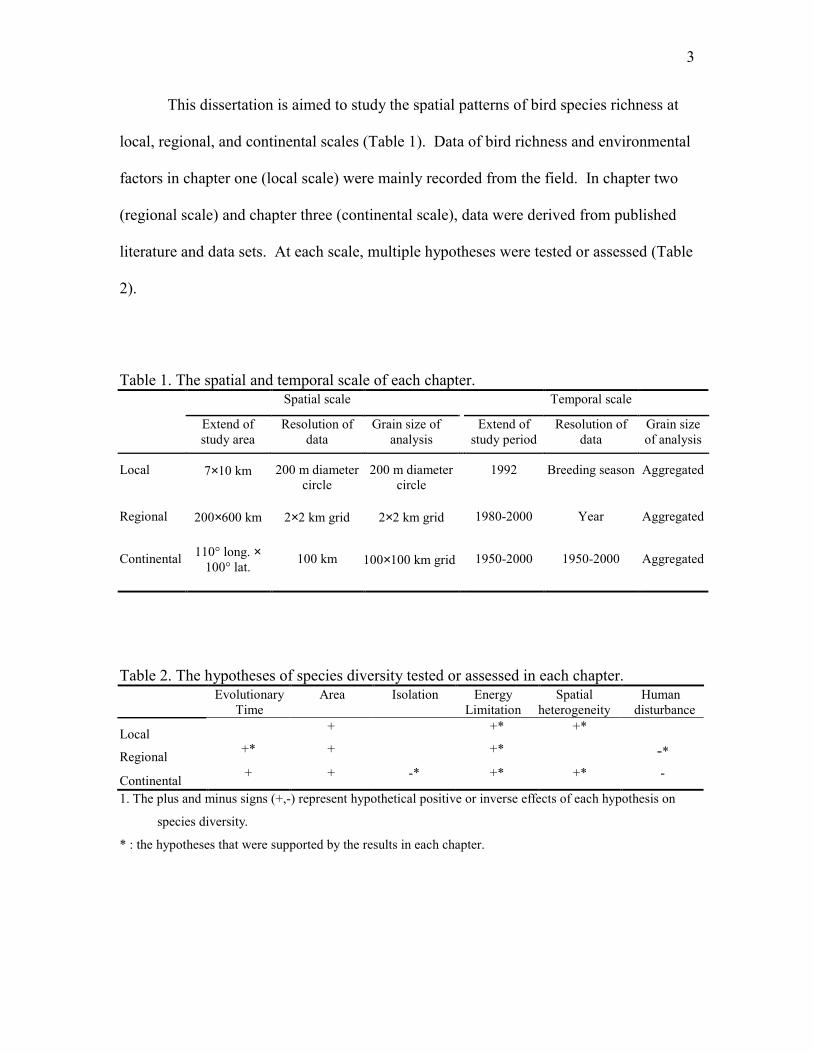
This dissertation is aimed to study the spatial patterns of bird species richness at

local, regional, and continental scales (Table 1). Data of bird richness and environmental

factors in chapter one (local scale) were mainly recorded from the field. In chapter two

(regional scale) and chapter three (continental scale), data were derived from published

literature and data sets. At each scale, multiple hypotheses were tested or assessed (Table

2).

Table 1. The spatial and temporal scale of each chapter.Spatial scale Temporal scale

Extend ofstudy area

Resolution ofdata

Grain size ofanalysis

Extend ofstudy period

Resolution ofdata

Grain sizeof analysis

Local 7×10 km 200 m diametercircle

200 m diametercircle

1992 Breeding season Aggregated

Regional 200×600 km 2×2 km grid 2×2 km grid 1980-2000 Year Aggregated

Continental 110° long. ×100° lat. 100 km 100×100 km grid 1950-2000 1950-2000 Aggregated

Table 2. The hypotheses of species diversity tested or assessed in each chapter.Evolutionary

TimeArea Isolation Energy

LimitationSpatial

heterogeneityHuman

disturbance

Local + +* +*

Regional +* + +* -*

Continental + + -* +* +* -

1. The plus and minus signs (+,-) represent hypothetical positive or inverse effects of each hypothesis on

species diversity.

* : the hypotheses that were supported by the results in each chapter.

4

The relationship between bird species richness (BSR) and elevation was a plateau-

then-decreasing relationship at the local scale and a hump-shaped relationship at the

regional scale. At the continental scale, BSR generally declined from the tropics to the

arctic. However, there were two minor exceptions in Mainland East Asia. BSR was

highest around Tropic of Cancer and it fluctuated between 30º and 50º N. Primary

productivity showed positive and strong correlation with BSR at all the spatial scales.

Spatial heterogeneity also showed positive correlation with BSR at the local and

continental scales. Evolutionary time theory was supported at the regional scale but was

rejected at the continental scale. After the sizes of analysis units (grains) were all

controlled to be equal at each scale, area only showed significant effect on the BSR of

isolated habitats (islands) at the continental scale and area theory was rejected at the local

scale, regional scale, and of mainland habitats at the continental scale. The effect of

isolation was examined and found significant at the continental scale. The effects of

human disturbance were tested at the regional and continental scales but found significant

only at the regional scale.

The energy limitation theory (Wright 1983) is strongly supported at all spatial

scales, suggesting that energy availability is one primary process of species diversity and

its effects may be consistent across spatial scales. The spatial heterogeneity theory

(MacArthur 1964) also has significant evidence at the local and continental scales.

However, at both scales its explanatory power is less significant than the energy limitation

theory. The evolutionary time theory (Fisher 1960), area theory (Rosenzweig 1992),

isolation theory (MacArthur and Wilson 1967), and human disturbance hypothesis have

gained some support at certain scales but their effects are not consistent across scales.

5

To search for explanations of species diversity, one needs to use evolutionary

arguments and to integrate our knowledge of population dynamics, species interactions,

landscape mosaics, and energy fluxes. It is not surprising that ecologists have yet

constructed a satisfactory conceptual framework on the processes and mechanisms of

species diversity. This dissertation intends to help the studies of species diversity in three

aspects. First, by integrating studies from various spatial scales and investigating

multiple hypotheses at each scale, it provides a holistic view and understanding of species

diversity. Second, it demonstrates how to take advantage of GIS and remotely sensed

data, which are respectively powerful tool and promising data source that have not been

fully utilized by ecologists. Third, it focuses on East Asia, where a large share of global

biodiversity is resided but has been traditionally under-reported and understudied by

ecologists.

Literature cited

Begon, M., J. L. Harper, and C. R. Townsend. 1990. Ecology: individuals, populations

and communities, 2nd ed. Blackwell Scientific Publications. Oxford, UK.

Blackburn, T. M. and K. J. Gaston. 1998. Some methodological issues in macroecology.

The American Naturalist 151:68-83.

Bohning-Gaese, K. 1997. Determinants of avian richness at different spatial scales.

Journal of Biogeography 24:49-60.

Brown, J. H. 1981. Two decades of homage to Santa Rosalia: towards a general theory of

diversity. American Zoologist 21:877-888.

6

Brown, J. H. 1988. Species diversity in Analytical biogeography ed. by A. A. Myers and

P. S. Giller. p. 57-89. Chapman and Hall, London, UK.

Brown, J. H. and M. V. Lomolino. 1998. Biogeography: 2nd edition. Sinauer, Sunderland,

MA, USA.

Connell, J. H. 1978. Diversity in tropical rainforests and coral reefs. Science 199:1302-

1310.

Connell, J. H. and E. Orians. 1964. The ecological regulation of species diversity.

American Naturalist 98:399-414.

Cornell, H. V. and J. H. Lawton. 1992. Species interactions, local and regional processes,

and limits to the richness of ecological communities: a theoretical perspective.

Journal of Animal Ecology 61:1-12.

Dobzhansky, T. 1950. Evolution in the tropics. American Naturalist 14:64-81.

Fischer, A. G. 1960. Latitudinal variations in organic diversity. Evolution 14:64-81.

Gaston, K. J. and T. M. Blackburn. 1999. A critique of marcoecology. Oikos 84:353-368.

Gaston, K. J. and T. M. Blackburn. 2000. Pattern and processes in macroecology.

Blackwell, Oxford, UK.

Hutchinson, G. E. 1959. Homage to Santa Rosalia, or why are there so many kinds of

animals? American Naturalist 93:145-159.

Levin, S. A. 1992. The problem of pattern and scale in ecology. Ecology 73:1943-1967.

MacArthur, R. H. 1964. Environmental factors affecting bird species richness. American

Naturalist 98: 387-398.

MacArthur. R. H. 1972. Geographical Ecology: patterns in the distribution of species.

Harper and Row. .New York. NY. USA.

7

MacArthur. R. H. and J. W. MacArthur. 1961. On bird species diversity. Ecology 42:594-

598.

MacArthur. R. H., and E. O. Wilson. 1967. The Theory of Island Biogeography.

Princeton University Press. Princeton, USA.

May, R. M. 1994. The effects of spatial scale on ecological questions and answers. in

Large-scale ecology and conservation biology ed. by P. J. Edwards, R. M. May,

and N. R. Webb. pp. 81-120. Blackwell. Oxford, UK.

O’Neill, R. V. 1989. Perspectives in hierarchy and scale. in Perspectives in ecological

theory ed. by J. Roughgarden, R. M. May and S. A. Levin. pp. 140-156.

Princeton University Press. Princeton, USA.

Paine, R. T. 1966. Food web complexity and species diversity. American Naturalist

100:65-75.

Ricklefs, R. E. 1987. Community diversity: relative roles of local and regional processes.

Science 235:167-171.

Ricklefs, R. E. 1990. Ecology, 3rd ed. Freeman. New York, USA.

Rosenzweig, M. L. 1992. Species diversity gradients: we know more and less than we

thought. Journal of Mammalogy 73:715-730.

Rosenzweig, M. L. 1995. Species diversity in space and time. Cambridge University

Press. Cambridge, UK.

Shmida, A and M. V. Wilson. 1985. Biological determinants of species diversity. Journal

of Biogeography 12:1-20.

Terborgh, J. 1973. On the notion of favorableness in plant ecology. American Naturalist

107:481-501.

8

Wiens, J. A. 1989. Spatial scaling in ecology. Functional Ecology 3:385-397.

Whittaker, R. J., K. J. Willis, and R. Field. 2001. Scale and species richness: toward a

general, hierarchical theory of species richness. Journal of Biogeography

28:453-470.

Wright, D. H. 1983. Species-energy theory: an extension of species-area theory. Oikos

41: 496-506.

9

Chapter One

Energy, Spatial Heterogeneity, and Rescue Effect on Bird Species

Richness along an Elevational Gradient in Yushan

10

Abstract

I examined the relationships of primary productivity, spatial heterogeneity, and

rescue effect with breeding bird species richness along a local elevational gradient in

Yushan, Taiwan. Bird species richness showed a plateau-then-decreasing relationship

with elevation and an increasing-then-plateau relationship with net primary productivity.

I further tested three mechanisms of the energy limitation theory and the results were

consistent with two of the predictions: bird total biomass was positively correlated with

net primary productivity, and bird species richness positively correlated with bird total

density. However, bird total density showed a hump-shaped relationship with bird total

biomass, which contradicts one prediction from the energy limitation theory. This result

implies more energy flux (estimated by bird total biomass) might decrease bird species

richness through increasing bird body size and reducing total density. Tree species

richness showed a hump-shaped relationship with elevation and was positively correlated

with bird species richness, supporting the spatial heterogeneity theory. One-kilometer

neighborhood area negatively correlated with bird species richness, indicating the rescue

effect is not significant. Results suggest that energy availability is possibly the ultimate

factor for bird species richness at this scale. For the decreasing phase of bird species

richness along the elevational gradient, the energy limitation theory well explains the

species richness. For the plateau phase, energy availability might be expressed through

multiple mechanisms in maintaining bird species richness. More energy availability

might indirectly decrease bird species richness through reducing bird total density and

spatial heterogeneity.

11

Introduction

Understanding spatial patterns of species richness has been one of the core theme

in ecology. Traditionally, species richness is expected to inversely correlate with

elevation, just as species richness declines from the tropics to the arctic (MacArthur

1972). That is, patterns of species richness along elevational gradients are considered as

mirrors of species richness along latitudinal gradients (Stevens 1992). Many papers

indeed report that there exists an inverse relationship between species richness and

elevation (e.g., Terborgh 1977, Able and Noon 1976, Patterson et al. 1998). Many

researchers (MacArthur 1972, Stevens 1992) think that changes of physical conditions

with latitude resemble the variations with elevation, and thus, such similarity drives the

similarity of species richness patterns on elevation and latitude. In a review of 90 data

sets that contain information on species richness of various taxa and elevational gradients

(Rahbek 1995), only 21% reported a monotonic decline of species richness on elevational

gradients, 49% reported a hump-shaped relationship, that is, peaking at intermediate

elevation range, and 25% showed a plateau-then-decreasing relationship. Rahbek (1995)

also suggested that some studies which reported a monotonically decreasing relationship

between species richness and elevational gradients actually would be hump-shaped if

their sampling efforts were standardized (e.g., Terborgh 1977). Rahbek (1995) further

pointed out that the climatic conditions among elevational gradients are not exactly

mirrors of latitudinal gradients. For instance, the dramatic seasonal temperature

differences in arctic and temperate regions are usually not observed on higher mountains

in tropical regions, although they are often referred to as arctic and temperate zones.

12

Also, most elevational gradients have a “humidity peak” that is not observed on

latitudinal gradients (Rahbek 1995). Besides, there is a fundamental difference between

these two types of gradients: elevational gradients are at local or regional scales, and

latitudinal gradients are at continental scale. Scale has been recognized as an important

factor that affects various ecological processes, which in turn determine the spatial

patterns of species richness (Shmida and Wilson 1985, Ricklefs 1987, Wiens 1989a,

O’Neill 1989, Levin 1992, Bohning-Gaese 1997, Caley and Schluter 1997, Goodwin and

Fahrig 1998, Gaston and Blackburn 1999, Lyons and Willig 1999). Therefore, patterns

of species richness on elevational gradients do not necessarily mirror latitudinal

gradients, and explanations for species richness on latitudes may not be considered

applicable to elevation considerations.

Taiwan, a small island, lies on the Tropic of Cancer with its highest elevation near

4000 meters. Steep elevational gradients are found within a short horizontal distance,

which makes it very suitable for studying species richness along elevational gradients.

Birds appear to be the best taxon for studying species richness in Taiwan because they are

diverse and well studied taxonomically. I chose to conduct this study at the local scale

rather than at the regional scale. The reasons are to: (1) minimize possible influences of

regional factors, (2) allow for a standardized sampling scheme, (3) to estimate bird

population densities accurately, and (4) to measure vegetation structure directly. The

objectives of this study are to examine the bird species richness patterns along an

elevational gradient and evaluate the following three most-discussed explanatory

theories: energy availability, spatial heterogeneity, and area size. These factors are

13

commonly considered as key factors that would define the underlying processes that in

turn determine and shape the species distribution patterns.

Earlier ecologists (Hutchinson 1959, Connell and Orias 1964, MacArthur 1965,

1972) proposed that energy availability limits the carrying capacity of a community to

contain species. Wright (1983) combined the energy concept with the island

biogeography theory (MacArthur and Wilson 1967) and suggested a species-energy

theory by replacing “area” with “energy availability” in the models of MacArthur and

Wilson (1967). This species-energy theory (energy limitation theory) suggests that the

increase of net primary productivity (NPP), i.e. gross primary productivity minus plant

total respiration, should increase the ability of plant community to support more

individuals of a consumer taxon per unit area. As the density of that consumer taxon

increases, population sizes increase, local extinction rates decrease, and thus species

richness of that consumer taxon increases. This energy limitation theory predicts a

positive relationship between NPP and species richness of a consumer taxon. This theory

has gained strong empirical and theoretical supports (Wright et al. 1993, Kaspari 2000).

However, recent evidence support a more complicated hump-shaped relationship (Grime

1973, Rosenzweig 1992, 1995, Rosenzweig and Abramsky 1993, Guo and Berry 1998).

That is, species richness increases with NPP at low levels of NPP, but decreases after

NPP reaches a certain level. Rosenzweig (1992, 1995) examined nine hypotheses for the

decreasing phase and concluded that there is no single convincing hypothesis that could

completely explain the decreasing phase of species richness on NPP. In this study, I

examined the relationship between NPP and bird species richness (BSR) and tested three

14

mechanisms of the energy limitation theory: (1) NPP increases bird total biomass, (2)

bird total biomass increases bird total density, and (3) bird total density increases BSR.

The spatial heterogeneity theory (MacArthur and MacArthur 1961, MacArthur

1964) has also been extensively studied by ecologists – especially avian ecologists. It

proposes that, if the spatial structure of a habitat is more complex, it should provide more

niches for more species, therefore species richness increases. The commonly used

indices of spatial heterogeneity for terrestrial birds at local are foliage height diversity

(MacArthur and MacArthur 1961) and plant species richness (Wiens 1989). The positive

relationship between BSR and spatial heterogeneity has been shown to hold within

several biogeographic regions (Terborgh 1977) and is often applied to explain patterns of

species richness along elevational gradients (MacArthur 1972). In this study, I measured

foliage height diversity and tree species richness and examined their relationships with

BSR.

The area-species relationship, a positive relationship between area size and

species richness, has been viewed as one of the most fundamental theories in ecology

(MacArthur 1972, Rosenzweig 1995, Ricklefs and Lovette 1999). If we divided

mountains into several equal-range elevational belts, the higher elevational belts would

usually have less area and greater isolation than lower elevational belts (Rahbek 1997).

Based on the island biogeography theory that a larger area has a lower extinction rate and

isolation restricts immigration, an inverse relationship between elevation and species

richness is therefore expected (MacArthur 1972). Although the importance of area effect

on species richness is widely documented, more than 50% of the studies of species

richness on elevational gradients did not justify the effect of area (Rahbek 1995).

15

Intuitively, taking sampling units of equal size along the elevational gradients could

eliminate the area effect. However, there are other area-related effects, especially when

animals are considered. A mountain can be viewed as composed of several elevational

habitat belts and islands and sampling units within larger habitat belts are generally

surrounded by larger area of similar habitats. If local populations of a sampling unit in a

larger habitat belt suffered disturbances and were locally extinct or nearly extinct, there

would be more individuals in the surrounding areas that could move in to rescue the

populations from local extinction and recover the species richness. This type of area-

related effect is called “rescue effect” (Brown and Kodric-Brown 1977). This rescue

effect is rarely discussed in studies dealing with area and species richness. In this study, I

estimated neighborhood area of each station and examined its relationship with BSR.

Neighborhood area is defined as area of similar habitats where birds can disperse into

each sampling station.

16

Study site

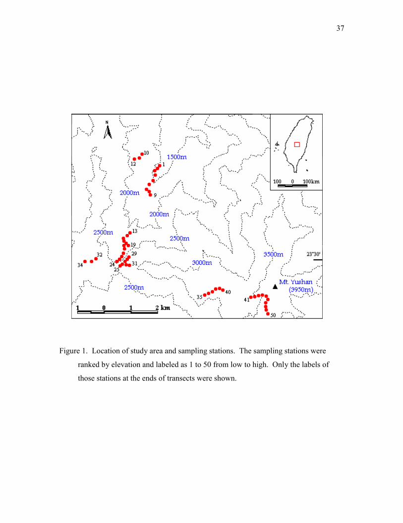
The study site was located on Mt. Yushan (23°28’30”N, 120°54’00”E) (3952 m

above sea level), the highest peak of Taiwan. Fifty sampling stations were selected and

ranged from 1400 to 3700 m (Figure 1). The selection criteria of sampling stations were:

(1) able to represent the typical climax plant communities along the elevation gradient,

(2) at least 100 m away from forest edges, creeks, and waterfalls, (3) at least 200 m away

from other sampling stations, (4) at least 200 m away from artificial constructions and

human-disturbed vegetation. The climatic variation and biotic communities along this

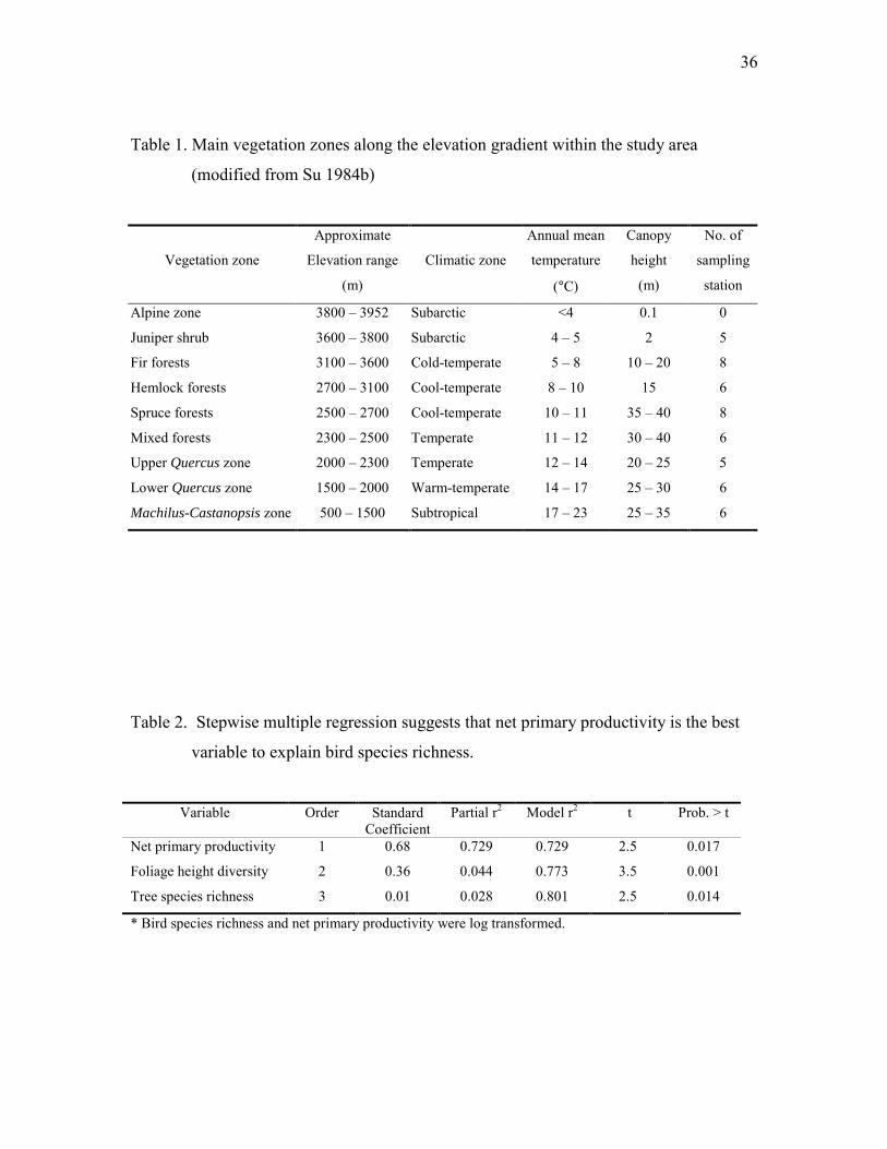
elevation gradient are similar to those from subtropical to sub-arctic climate zones (Table

1).

Weather data of 32 weather stations within or near the study site show that annual

average temperature decreases 5.29 °C for every 1000 meter elevation (r2 = 0.96) (Su

1984a). This relationship holds well for different seasons (Su 1984a). In the study site,

snow falls frequently above 2000 m and the snow season could last one to four months

above 3000 m. Precipitation in the study site is mainly affected by the summer

southwestern monsoon. Summer rainfall (April to September) accounts for 80-85% of

the annual precipitation and shows a hump-shaped relationship with elevation. From sea

level, summer rainfall tends to increase with elevation, usually reaches its maximum

around 2200 m, and then decreases with elevation (Su 1984a). Winter precipitation

(October to March), brought by the northeastern monsoon, only accounts 10%-15% of

annual precipitation and is linearly and positively correlated with elevation (slope =

135.5mm/km, r = 0.88) due to rain shadow effect (Su 1984a).

17

Population density is very high in Taiwan (609 persons per square kilometer as of

July, 2000). Most of the old-growth forests below 1300 m have been converted into

agricultural farms or sylvicultural plantations. In a previous study (Ding et al. 1997)

showed that vegetation succession strongly affects the species richness and composition

of bird communities in this area. In order to exclude the effect of disturbance and

succession, this study was conducted only in the areas of undisturbed climax plant

communities, which form several vegetation zones along the elevational gradient (Table

1). The timberline lies around 3600 m. Shrubs of juniper and rhododendron are most

prevalent between the timberline and 3800 m. Pure stands of fir dominate under the

timberline down to 3100 m. Hemlock forests are distributed between 3100 and 2700 m.

In both forest types, secondary trees are generally absent and dense bamboo shrubs

overwhelm the forest floor. Spruce forests dominate between 2700 m and 2500 m.

Secondary trees are primarily broadleaf trees. On the forest floor, bamboo shrubs are

replaced by ferns and herbs. Between 2500 and 2300 m, conifer trees dominate the

canopy layer which account for 30% to 70% of the canopy. The secondary tree layer (5-

10 m tall) is closed and dominated by various broadleaf trees. Below 2300 m, coniferous

trees disappear and broadleaf evergreen trees (mostly Fagaceae and Lauraceae) become

dominant. Based on tree composition and ground vegetation type, the broadleaf forests

are divided into three zones: upper Quercus zone, lower Quercus zone, and Machilus-

Castanopsis zone (Su 1984b). The canopy, secondary tree, shrub, and herb layers of those

zones are well developed and rich in floristic composition.

18

Methods

Estimation of bird densities and total biomass

Bird species densities were estimated from March to July 1992 by using the

variable circular-plot sampling method (Reynolds et al. 1980). A pilot study determined

the optimal time of bird count, which is a six-minute counting interval per hour for four

hours after sunrise. At each station, I recorded the number, distance, sex (by appearance

or song) of all bird individuals seen or heard during the six-minute period of every hour.

The timing of field counts was designed to correspond to the time lag of bird breeding

seasons along the elevational gradient. Bird counts on stations below 2000m were started

in late-March and ended in late-May; on stations between 2000m and 3000m were

counted from early-April to late-June; and on stations above 3000m were counted

between mid-May and early-July. At each sampling station, I counted 16 times for a total

of 96 minutes.

The mean body mass data of all breeding bird species in Taiwan (Lee et al. 1999)

were combined with bird densities to calculate the bird total biomass at each sampling

station.

Estimation of primary productivity

Net primary productivity (NPP) was estimated from weather data. Monthly mean

temperature and precipitation at each sampling station were approximated by using the

1961-1990 average monthly weather data of the weather stations within or close to the

study site. These estimates were adjusted by elevation, using the models reported by Su

19

(1984a). Evapotranspiration (ET) of each station was estimated by the monthly mean

temperature and precipitation, using the tables and equations of Thornthwaite and Mather

(1957). ET is the amount of water returned to atmosphere through evaporation and

transpiration. It correlates well with the photosynthetic activity of plants and has been

used as an estimate of NPP (e.g., Currie 1991, Rosenzweig 1995). I estimated annual net

aboveground primary productivity of each sampling station by the model of Rosenzweig

(1968), log10NPP = 1.7003·log10ET – 1.7661, which explains 90% of net aboveground

primary productivity in undisturbed habitats worldwide.

Measurement of spatial heterogeneity indices

In the study site, most of the sampling stations had slopes greater than 30º and the

precipitous topography prevented researchers from moving freely in the forests. The

original methods used to measure foliage height diversity (FHD) (MacArthur and

MacArthur 1961) were therefore difficult in this study. A simplified measurement of

foliage volume and FHD was employed. I estimated foliage coverage (0-100%) of four

layers (0-0.6m, 0.9-1.8m, 3-6m, and 10-15m) in a 40m diameter circle at each station in

the summer of 1992. The four layers represented herb, shrub, sub-canopy, and canopy

layers of forests. Foliage height diversity was calculated using the Shannon-Wiener

Index (Magurran 1988) of the foliage coverage of the four layers. In addition, I counted

trees (diameter at breast height > 1cm) within a 20m diameter circle at each sampling

station to calculate tree species richness (TSR).

Estimation of neighborhood area

20

Barrowclough (1980) summarized several field studies and concluded that,

exclusive of seasonal migration, non-colonial passerine birds disperse roughly one

kilometer per year, with a range of 350 to 1700 meters per year. The available bird

banding data in Taiwan were in agreement with Barrowclough’s (1980) estimation.

Since this study covered only one breeding season, I chose one kilometer as the buffer

distance to test the rescue effect. Using ARC/INFO, I created point coverage of the 50

sampling stations and then established circular buffer zones centered at each of the

stations with a diameter of two kilometers. Those circular-shaped buffers were further

overlaid with digital elevation model (DEM) coverage of Taiwan (40 × 40m resolution).

The neighborhood area of each station was calculated as the area of grids that falls within

the corresponding buffer zone and within 100 m elevation difference from the station.

21

Results

Bird species richness, density, and biomass

I recorded 59 breeding species from 13,716 individual records in the field bird

counts. Based on the Sibley-Ahlquist-Monroe avian taxonomy system (Monroe and

Sibley 1993), 46 species (78%) were passerines and the largest family (18 species) was

Sylviidae (babblers and warblers). All the species recorded were non-colonial and

showed some territory behaviors during the period of field bird counts.

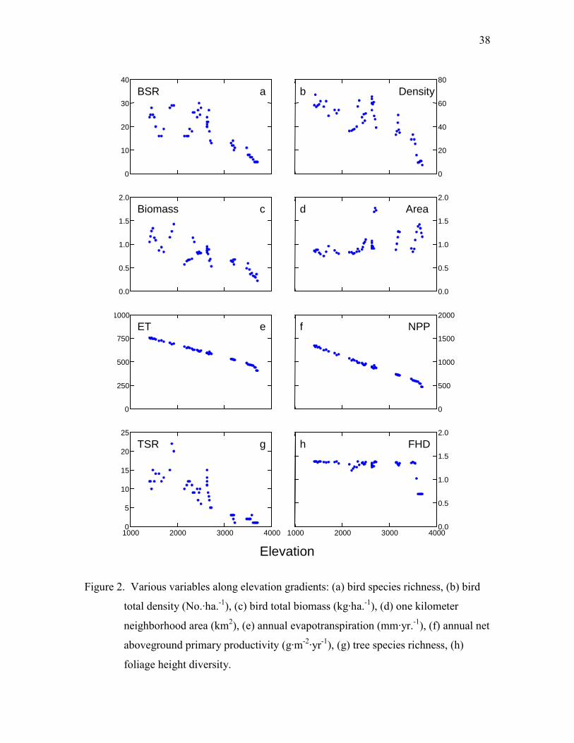
Bird species richness (BSR) did not monotonically decline nor show a hump-

shaped relationship with elevation. BSR curve was roughly equal across in broadleaf

forests with considerable variation (16-29 species), reached its maximum (30 species) in

mixed forests, then monotonically declined in conifer forests, and reached minimum in

juniper shrubs (5-6 species) (Fig. 2a). Bird total density was high in broadleaf forests,

mixed forests, and spruce forests (67.1 - 36.2 No. ha.-1), then deceased with elevation,

and was the lowest in juniper shrubs (7.3 - 10.9 No. ha.-1) (Fig. 2b). Bird total biomass

monotonically declined with elevation (1.43 - 0.22 kg ha.-1) and had higher variation at

lower elevations (Fig. 2c).

ET and NPP

The estimated annual ET linearly and inversely correlated with elevation and

ranged from 752 to 407 (mm yr-1) along the gradient (Fig. 2e). Although summer (April

– September) precipitation had a hump-shaped relationship with elevation, the amount of

rainfall was never a limiting factor for ET in summer. For instance, the summer

22

precipitation was greater than 2400 mm in all locations. Temperature, which was linearly

and inversely correlated with elevation, was the limiting factor for ET. NPP also linearly

and inversely correlated with elevation and ranged from 466 to 1343 (g m-2 yr-1) along the

gradient (Fig. 2f). These estimations were consistent to those reported by Lieth and

Whittaker (1975) on similar vegetation types worldwide.

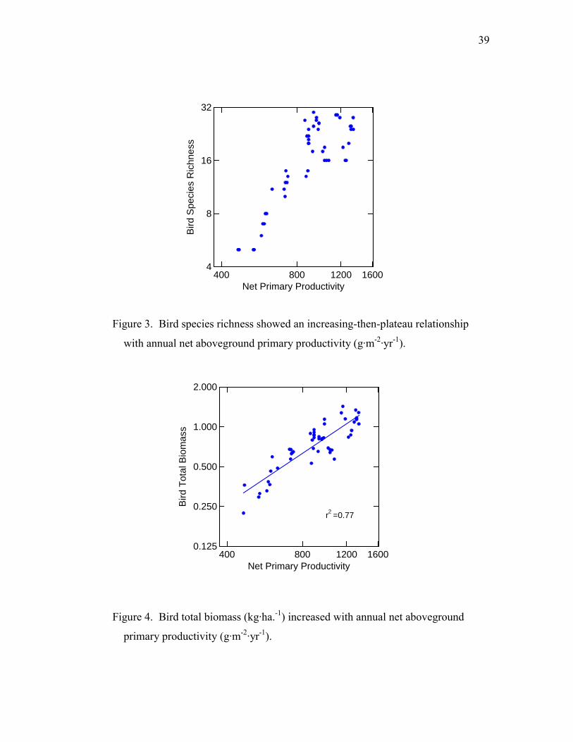
After the double log transformation, BSR positively correlated with NPP (slope =

1.58, F = 128.5, p < 0.001, R2 = 0.73) (Fig. 3). In a polynomial regression analysis of

NPP and BSR, both quadratic and cubic factors were significant (p < 0.01), suggesting

BSR was not linearly related to NPP. In order to test whether it was hump-shaped or an

increasing-then-plateau relationship, I subjected sampling stations 1-22 (station 22 had

the highest BSR and stations 1-22 had higher NPP) to a linear regression analysis. The

result was not significant (F = 0.006, p = 0.94), implying an increasing-then-plateau

relationship between NPP and BSR.

If the energy limitation theory is correct, the following three relationships should

be observed. First, NPP increases bird total biomass. Second, bird total biomass

increases bird total density. Third, bird total density increases BSR. In my analysis, bird

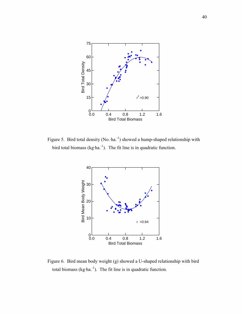
total biomass was positively and linearly correlated with NPP when both variables were

log transformed (r2 = 0.77, F = 158.0, p < 0.001) (Fig. 4). However, bird total density

showed a humped-shape relationship with bird total biomass (Fig. 5), which contradicted

the second prediction from the energy limitation theory. Bird total biomass explained

90% of the variance of bird total density in a quadratic regression model (t = -9.01, p <

0.001, for the quadratic factor) (Fig. 5). The bird mean body weight (bird total biomass

divided by bird total density) showed a U-shaped relationship with bird total biomass

23

(Fig. 6). In a quadratic polynomial regression, bird total biomass explained 64% of the

variance of bird mean body weight (t = -8.99, p < 0.001, for quadratic factor) (Fig. 6).

Thus, on average, birds tended to be smaller at intermediate levels of NPP (elevation).

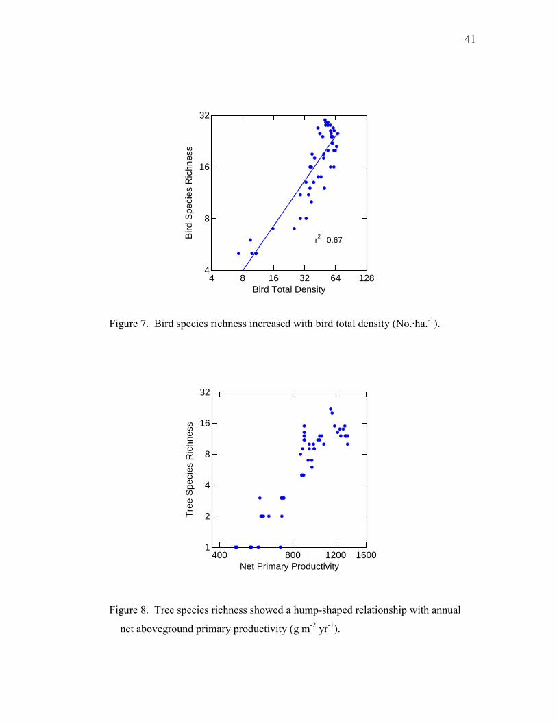
The relationship between density and richness, however, was consistent to the third

prediction of the energy limitation theory. Bird total density positively and linearly

correlated with BSR after both variables were log transformed (r2 = 0.78, F = 170.5, p <

0.001) (Fig. 7).

Parameters of plant communities

TSR ranged from 1 to 22 species (within a circular area of 314m2) and showed a

hump-shaped relationship with elevation (p < 0.01, for quadratic and cubic factors of

polynomial regression) (p < 0.05, for the negative slope of linear regression of sampling

stations 1-11) (Fig. 2g). Along the elevational gradient, TSR increased first, peaked

around 2000 m, and gradually declined with elevation. FHD was lowest in juniper shrubs

and roughly remained constant at a high level in other forests along the gradient (Fig. 2h).

TSR showed a hump-shaped relationship with NPP (Fig. 8). NPP explained 84%

of the variation in TSR in the polynomial regression model (F = 71.4 for quadratic and

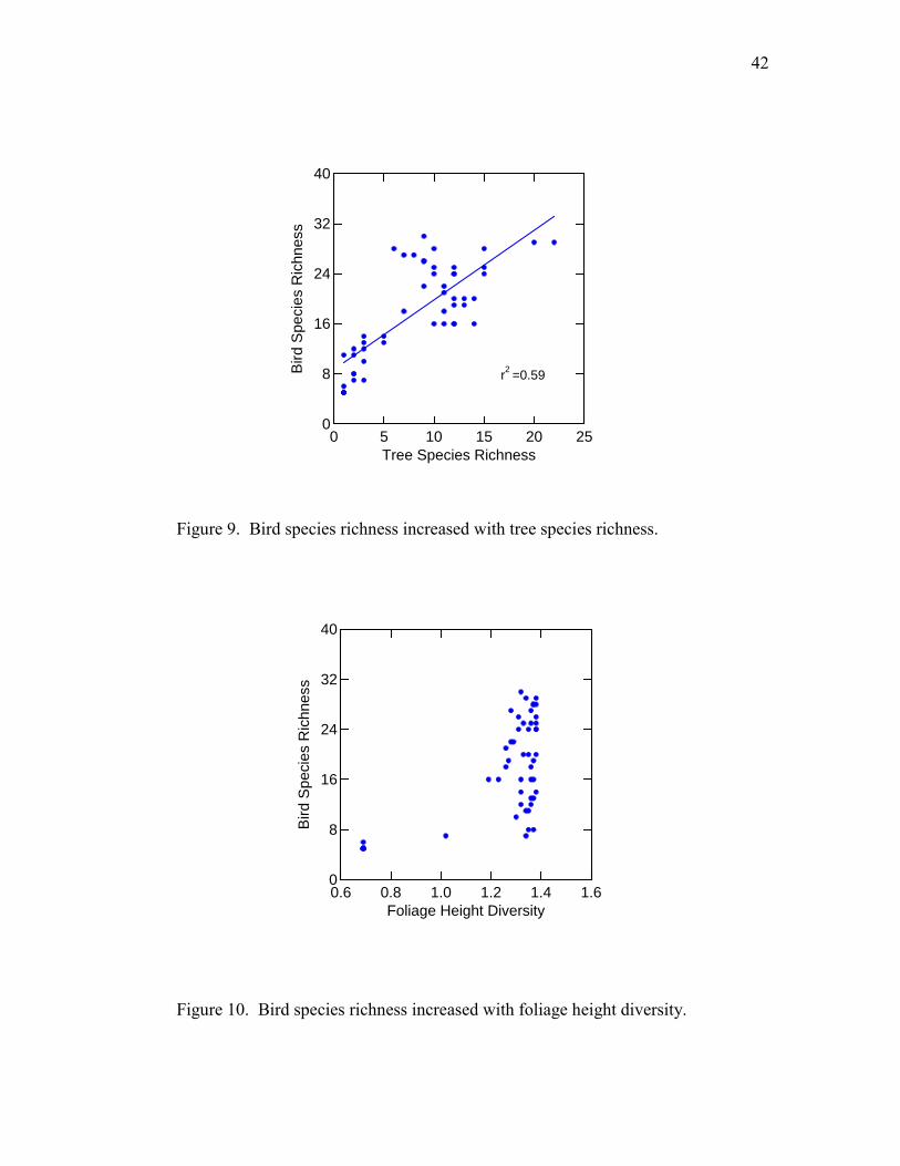
cubic factors and p < 0.001). BSR significantly and positively correlated with TSR (r2 =

0.59, F = 69.7, p < 0.001) (Fig. 9) and FHD (r2 = 0.35, F = 26.2, p < 0.001) (Fig. 10).

Neighborhood area

The 1 km neighborhood area did not vary consistently with elevation (Fig. 2d).

BSR was significantly but negatively correlated with neighborhood area in a simple

24

regression after both variables were log transformed (slope = -1.28, r2 = 0.26, F = 17.0, p

< 0.001). The rescue effect predicts the slope of regression function (z) be significantly

greater than zero. Thus the rescue effect hypothesis was rejected at this scale.

Multiple regressions

Stepwise multiple regression (criteria for inclusion and exclusion, p < 0.05) was

applied to evaluate the effects of NPP, TSR, FHD, and neighborhood area on BSR. NPP,

neighborhood area, and BSR were log-transformed to meet the normality and variance

homogeneity assumptions of the regression analysis. NPP explained 73% of variance in

BSR (p < 0.001), FHD explained additional 4% (p = 0.004), and TSR explained

additional 3% (p = 0.014) (Table 2). Neighborhood area was excluded in the final model

for its insignificant contribution to the model.

25

Discussion

In this study, BSR plateaued at lower elevations but then declined at higher

elevations. Would the BSR remain a plateau, or decline, or increase if the elevational

gradient was extended to sea level? This question is virtually impossible to answer in this

study because most of the habitats below 1300 m in this region have been extensively

modified by human activities. In another study (chapter two), BSR of 674 localities in

Taiwan was compiled from 288 avifauna censuses that covered one or two years of

census period. BSR and elevation showed a hump-shaped relationship along the entire

elevational gradient in Taiwan. BSR was highest between 1400 to 2200 m. Although the

massive agricultural and urban land uses on Taiwan’s lowlands might contribute to this

hump-shaped relationship; it was also observed that some lowland old-growth forests had

significantly fewer bird species than mid-elevation forests. I thus conclude that BSR

would not likely increase if I extended the elevational gradient to the lowlands.

Rahbek (1995) argues that species richness patterns on elevational gradients do

not necessary mirror latitudinal gradients. He also pointed out that 79% of the cases did

not standardize the effect of area and sampling effort, which might distort the actual

relationship between species richness and elevation. I employed a sampling scheme of

same area and sampling effort. The observed plateau-then-decreasing relationship

supports Rahbek’s (1995) argument that the monotonically inverse relationship of species

richness and elevation is not as universal as ecologists generally assume.

26

Energy availability

BSR showed an increasing-then-plateau relationship with NPP. Testing further, I

found the results contradict one of the underlying mechanisms. Here I discuss those

mechanisms in detail.

First, if energy availability is a limiting factor for species richness, the energy flux

into a consumer taxon or trophic group should be proportional to the available energy.

That is, the consumer group must be able to exploit more energy if there are more

resources available. I used bird total biomass as the index of energy flux. The high

correlation between bird biomass and the estimated NPP suggests that the energy

consumed by birds is proportional to NPP. This result is consistent with the prediction of

the first mechanism of energy limitation theory.

Bird total biomass is not only a reasonable index of energy flux but also possibly

a more accurate estimation of NPP that ET. The primary productivity or the energy fixed

by photosynthesis is extremely difficult to measure directly. In this study, I collected

weather data to estimate NPP through ET, an approach that is popular among ecologists.

The result showed a general trend of NPP along the elevational gradient. However, some

on-site variations were not accounted in the smooth NPP line along elevational gradient.

Although temperature and precipitation played a predominant role in NPP, other

environmental factors such as slope, aspect, and soil properties also affect NPP.

Estimating NPP solely from weather data may not sufficiently reflect the variation in

NPP that could be caused by other important habitat properties. As a result, I suggest

bird total biomass is a better estimator of NPP in this case.

27

Second, if energy availability is a limiting factor for species richness, total density

of a consumer group should be proportional to its energy flux. My results do not support

this prediction. Bird total density showed a hump-shaped relationship with bird total

biomass. Bird density first increased with bird total biomass and decreased after bird

total biomass roughly reached one kilogram per hectare. I also observed a U-shaped

relationship between bird mean body weight (per individual) and bird total biomass. It is

difficult to determine whether this U-shaped relationship was attributed to energy

availability, climate, or a combination of both, since mean air temperature also correlated

well with bird total biomass in this study.

The third mechanism of the energy limitation theory predicts that species richness

be proportional to total density. That is, higher density reduces the possibility of local

extinction and thus increases species richness. I found BSR increased with bird total

density, which is consistent with the prediction.

In short, the hump-shaped relationship between BSR and NPP was not observed.

However, I found a hump-shaped relationship between bird total biomass and total

density, which contradicted to one of the underlying mechanisms of the energy limitation

theory.

One intriguing pattern in species richness is the hump-shaped relationship

between primary productivity and species richness, which has accumulated considerable

empirical support in recent years. However, there is no theoretical model that predicts

where the peak of hump-shaped relationship occurs. The positive relationship between

primary productivity and species richness has often been explained as part (the increasing

phase) of the hump-shaped relationship (e.g., Rosenzweig 1992, 1995, Rosenzweig and

28

Abramsky 1993, Guo and Berry 1998). The observed relationship between NPP and

BSR in this study is also difficult to attribute as whole or part of the pattern.

Nevertheless, the observed hump-shaped relationship between bird total biomass and

total density hints one possible explanation of the decreasing phase of the hypothetical

hump-shaped relationship. That is, once energy availability reaches a certain level, it

might decrease species richness through increasing body size and reducing total density.

Rosenzweig (1992, 1995) discussed nine hypotheses explained the decreasing phase of

species richness on NPP. However, the observed hump-shaped relationship between total

biomass and total density can not properly fit any of the nine hypotheses. The

relationships among primary productivity, body size, density, and species richness are

important topics warranting further investigation.

Spatial heterogeneity

The spatial heterogeneity theory postulates that a more complex habitat provides

more niches that would allow more species to inhabit it. In this study, I chose FHD and

TSR to represent the degree of spatial heterogeneity of the sampling stations. FHD

represents the vertical and structural heterogeneity of vegetation, and plant species

richness represents the horizontal and floristic heterogeneity of vegetation. Since all the

sampling stations were located within climax vegetation, there was not much variance in

FHD. Most of the variation came from structural differences between forests and juniper

shrubs. Because of the narrow variation of FHD, I did not find a clear relationship

between BSR and FHD.

29

TSR correlated well with BSR. This result is consistent with former studies (e. g.

Karr and Roth 1971, Rice et al. 1983). TSR also showed a significant hump-shaped

relationship with elevation and NPP. The hump-shaped relationship of TSR on NPP,

along with other factors, might be one of the reasons for the observed plateau-then-

decreasing relationship of BSR on elevation. Many papers reported that species richness

has a hump-shaped relationship with primary productivity (or energy availability).

Rosenzweig (1992, 1995) concluded that environmental heterogeneity (Tilman 1982) is

one of the most plausible hypotheses that explain the decreasing phase of species richness

on NPP but it is probably tautology because spatial heterogeneity might co-evolve with

species richness. I did not design this study to explore the processes of TSR; therefore, it

is difficult to speculate on the mechanisms for the hump-shaped relationship between

TSR and NPP. However, TSR is a reasonable index for environmental heterogeneity

from birds’ standpoint and it correlated well with BSR, which supported the

environmental heterogeneity hypothesis. Although birds might facilitate TSR through

pollination and seed dispersal, it is not very convincing that BSR plays a prominent role

for TSR. Therefore, the concern about tautology might not be important in this case.

Rescue effect

Ecologists often view area effect as a primary process for spatial patterns of

species richness (e.g., Rosenzweig 1995). In this study, each sampling station had the

same area size and the neighborhood area was not a factor for species richness. There is

no direct evidence that area size is responsible for the observed species richness patterns

in this study.

30

In summary, I found that: firstly, BSR showed a plateau-then-decreasing

relationship with elevation; secondly, area was not a factor at this (local) scale; and

thirdly, energy availability played an important role and possibly provided the ultimate

explanation for BSR in this study. Energy limitation theory explains well the decreasing

phase of BSR on elevation. For the plateau phase of BSR on elevation, more energy

availability may have indirectly decreased BSR through the reduction of bird total density

and spatial heterogeneity.

31

Literature cited

Able, K. P. and B. R. Noon. 1976. Avian community structure along elevational gradients

in the northeastern United States. Oecologia 26: 275-294.

Barrowclough, G. F. 1980. Gene flow, effective population size, and genetic variance

components in birds. Evolution 34: 789-798.

Brown, J. H. and A. Kodric-Brown. 1977. Turnover rates in insular biogeography: effect

of immigration on extinction. Ecology 58: 445-449.

Connell, J. H. and E. Orias. 1964. The ecological regulation of species diversity.

American Naturalist 98: 399-414.

Currie, D. J. 1991. Energy and larger-scale patterns of animal and plant species richness.

American Naturalist 137: 27-49.

Ding, T. S., P F. Lee, and Y. S. Lin. 1997. Avian distribution pattern of highland areas in

Central Taiwan. Acta Zoologica Taiwanica 8: 55-64.

Grime, J. P. 1973. Control of species density in herbaceous vegetation. Journal of

Environmental Management 1: 151-167.

Guo, Q. and W. Berry. 1998. Species richness and biomass: dissection of the hump-

shaped relationships. Ecology 79: 2555-2559.

Hutchinson, G. E. 1959. Homage to Santa Rosalia, or why are there so many kinds of

animals? American Naturalist 93: 145-159.

Karr, J. R. and R. R. Roth. 1971. Vegetation structure and avian diversity in several New

World areas. American Naturalist 105: 423-435.

32

Kaspari, M. S., O’Donnell, and J. R. Kercher. 2000. Energy, density, and constraints to

species richness: ant assemblages along a productivity gradient. American

Naturalist 155: 280-293.

Lee, P. F., T. S. Ding, and H. J. Shiu. 1999. Body size relation of breeding bird species in

Taiwan. Acta Zoologica Taiwanica 9: 47-59

Lieth, H. and R. H. Whittaker. (eds.) 1975. Primary productivity of the biosphere.

Springer. New York, USA.

MacArthur, R. H. 1964. Environmental factors affecting bird species richness. American

Naturalist 98: 387-398.

MacArthur, R. H. 1965. Patterns of species richness. Biological Reviews 40: 510-533.

MacArthur, R. H. 1972. Geographical Ecology: patterns in the distribution of species.

Harper & Row. New York, USA.

MacArthur, R. H. and J. W. MacArthur. 1961. On bird species diversity. Ecology 42:

594-598.

MacArthur, R. H. and E. O. Wilson. 1967. The theory of island biogeography. Princeton

University Press. Princeton, USA.

Magurran, A. E. 1988. Ecological diversity and its measurement. Princeton University

Press. Princeton, USA.

Monroe, B. L. and C. G. Sibley. 1993. A world checklist of birds. Yale University Press.

New Heaven, USA.

Patterson, B. D., D. F. Stotz, S. Solari, J. W. Fitzpatrick, and V. Pachecom. 1998.

Contrasting patterns of elevational zonation for birds and mammals in the Andes

of southeastern Peru. Journal of Biogeography 25: 593-607.

33

Rahbek, C. 1995. The elevational gradient of species richness: a uniform pattern?

Ecography 18: 200-205.

Rahbek, C. 1997. The relationship among area, elevation, and regional species richness in

Neotropical birds. American Naturalist 149: 875-902.

Reynold, R. T., M. Scott, and R. A. Nussbaum. 1980. A variable circular-plot method for

estimating bird numbers. Condor 82: 309-313.

Rice, J. R., D. Ohmart, and B. W. Anderson. 1983. Habitat selection attributes of an avian

community: a discriminant analysis investigation. Ecological Monographs 53:

263-290.

Ricklefs, R. E. and I. J. Lovette. 1999. The roles of island area per se and habitat diversity

in the species-area relationships of four Lesser Antillean faunal groups. Journal

of Animal Ecology 68: 1142-1160.

Rosenzweig, M. L. 1968. Net primary productivity of terrestrial communities: predictions

from climatological data. American Naturalist 102: 67-74.

Rosenzweig, M. L. 1992. Species diversity gradients: we know more and less than we

thought. Journal of Mammalogy 73: 715-730.

Rosenzweig, M. L. 1995. Species diversity in space and time. Cambridge University

Press. Cambridge, UK.

Rosenzweig, M. L. and Z. Abramsky. 1993. How are diversity and productivity related?

In: Ricklefs, R. E. and Schluter, D. (eds.), Species diversity in ecological

communities: historical and geographical perspectives. University of Chicago

Press, pp. 52-65. Chicago, USA.

34

Stevens, G. C. 1992. The elevational gradient in altitudinal range: an extension of

Rapoport’s latitudinal rule to altitude. American Naturalist 140: 893-911.

Su, H. J. 1984(a). Studies on the climate and vegetation types of the natural forests in

Taiwan(I): analysis of the variations on climatic factors. Quarterly Journal of

Chinese Forestry 17: 1-14.

Su, H. J. 1984(b). Studies on the climate and vegetation types of the natural forests in

Taiwan(II): altitudinal vegetation zones in relation to temperature gradient.

Quarterly Journal of Chinese Forestry 17: 57-73.

Terborgh, J. 1977. Bird species diversity on an Andean elevation gradient. Ecology 58:

1007-1019.

Thornthwaite, C. W. and J. R. Mather. 1957. Instructions and tables for computing

potential evapotranspiration and the water balance. Publications in Climatology

10: 185-311.

Tilman, D. 1982. Resource competition and community structure. Princeton University

Press. Princeton, USA.

Tilman, D. and S. Pacala. 1993. The maintenance of species richness in plant

communities. In: Ricklefs, R. E. and Schluter, D. (eds.), Species diversity in

ecological communities: historical and geographical perspectives. University of

Chicago Press, pp. 13-25. Chicago, USA.

Wiens, J. A. 1989. The ecology of bird communities. Vol. 1: Foundations and patterns.

Cambridge University Press. Cambridge, UK.

Wright, D. H. 1983. Species-energy theory: an extension of species-area theory. Oikos

41: 496-506.

35

Wright, D. H., D. J. Currie, and R. A. Maurer. 1993. Energy supply and patterns of

species richness on local and regional scales. In: Ricklefs, R. E. and Schluter, D.

(eds.), Species diversity in ecological communities: historical and geographical

perspectives. University of Chicago Press, pp. 66-74. Chicago, USA.

36

Table 1. Main vegetation zones along the elevation gradient within the study area

(modified from Su 1984b)

Vegetation zone

Approximate

Elevation range

(m)

Climatic zone

Annual mean

temperature

(°C)

Canopy

height

(m)

No. of

sampling

station

Alpine zone 3800 – 3952 Subarctic <4 0.1 0

Juniper shrub 3600 – 3800 Subarctic 4 – 5 2 5

Fir forests 3100 – 3600 Cold-temperate 5 – 8 10 – 20 8

Hemlock forests 2700 – 3100 Cool-temperate 8 – 10 15 6

Spruce forests 2500 – 2700 Cool-temperate 10 – 11 35 – 40 8

Mixed forests 2300 – 2500 Temperate 11 – 12 30 – 40 6

Upper Quercus zone 2000 – 2300 Temperate 12 – 14 20 – 25 5

Lower Quercus zone 1500 – 2000 Warm-temperate 14 – 17 25 – 30 6

Machilus-Castanopsis zone 500 – 1500 Subtropical 17 – 23 25 – 35 6

Table 2. Stepwise multiple regression suggests that net primary productivity is the best

variable to explain bird species richness.

Variable Order StandardCoefficient

Partial r2 Model r2 t Prob. > t

Net primary productivity 1 0.68 0.729 0.729 2.5 0.017

Foliage height diversity 2 0.36 0.044 0.773 3.5 0.001

Tree species richness 3 0.01 0.028 0.801 2.5 0.014

* Bird species richness and net primary productivity were log transformed.

37

Figure 1. Location of study area and sampling stations. The sampling stations were

ranked by elevation and labeled as 1 to 50 from low to high. Only the labels of

those stations at the ends of transects were shown.

38

Figure 2. Various variables along elevation gradients: (a) bird species richness, (b) bird

total density (No.·ha.-1), (c) bird total biomass (kg·ha.-1), (d) one kilometer

neighborhood area (km2), (e) annual evapotranspiration (mm·yr.-1), (f) annual net

aboveground primary productivity (g·m-2·yr-1), (g) tree species richness, (h)

foliage height diversity.

0

10

20

30

40

0

20

40

60

80

0.0

0.5

1.0

1.5

2.0

0.0

0.5

1.0

1.5

2.0

0

250

500

750

1000

0

500

1000

1500

2000

1000 2000 3000 40000

5

10

15

20

25

1000 2000 3000 40000.0

0.5

1.0

1.5

2.0

BSR Density

Biomass Area

ET NPP

TSR FHD

Elevation

a b

c d

e f

g h

39

Figure 3. Bird species richness showed an increasing-then-plateau relationship

with annual net aboveground primary productivity (g·m-2·yr-1).

Figure 4. Bird total biomass (kg·ha.-1) increased with annual net aboveground

primary productivity (g·m-2·yr-1).

400 800 1200 1600Net Primary Productivity

4

8

16

32

Bird

Spe

cies

Ric

hnes

s

400 800 1200 1600Net Primary Productivity

0.125

0.250

0.500

1.000

2.000

Bird

Tot

al B

iom

a ss

r =0.772

40

Figure 5. Bird total density (No.·ha.-1) showed a hump-shaped relationship with

bird total biomass (kg·ha.-1). The fit line is in quadratic function.

Figure 6. Bird mean body weight (g) showed a U-shaped relationship with bird

total biomass (kg·ha.-1). The fit line is in quadratic function.

0.0 0.4 0.8 1.2 1.6Bird Total Biomass

0

15

30

45

60

75

Bird

Tot

al D

ens i

ty

r =0.902

0.0 0.4 0.8 1.2 1.6Bird Total Biomass

0

10

20

30

40

Bird

Mea

n Bo

d y W

eigh

t

r =0.64

41

Figure 7. Bird species richness increased with bird total density (No.·ha.-1).

Figure 8. Tree species richness showed a hump-shaped relationship with annual

net aboveground primary productivity (g m-2 yr-1).

400 800 1200 1600Net Primary Productivity

1

2

4

8

16

32

Tree

Spe

cies

Ric

hnes

s

4 8 16 32 64 128Bird Total Density

4

8

16

32

Bird

Spe

cies

Ric

hnes

s

r =0.672

42

Figure 9. Bird species richness increased with tree species richness.

Figure 10. Bird species richness increased with foliage height diversity.

0 5 10 15 20 25Tree Species Richness

0

8

16

24

32

40

Bir d

Spe

cies

Ric

h nes

s

r =0.592

0.6 0.8 1.0 1.2 1.4 1.6Foliage Height Diversity

0

8

16

24

32

40

Bir d

Spe

cies

Ric

h nes

s

43

Chapter Two

Breeding Bird Species Richness on Gradients of Elevation,

Primary Productivity, and Human Disturbance in Taiwan

44

Abstract

I examined the distribution patterns of breeding bird species richness on gradients

of elevation, primary productivity, and human disturbance in Taiwan. Bird species

richness (BSR) data were compiled from avifauna censuses undertaken in 288 sites in

Taiwan from 1980 to 2000. BSR showed a hump-shaped relationship with elevation,

increased with primary productivity, and decreased with human disturbance. Further

analyses revealed that human disturbance decreased with elevation. In addition, primary

productivity showed a hump-shaped relationship with elevation and decreased with

human disturbance. Multiple regression analysis showed that linear and cubic terms of

elevation explained 31.3% of the variation in BSR and human disturbance explained

additional 3.4%. The explanatory power of primary productivity was insignificant after

the effects of elevation and human disturbance were justified. Results showed that

human disturbance is a main reason that BSR increased with elevation in the lower

elevations of Taiwan. Furthermore, the biotic communities in the mid-elevation zone had

relatively longer periods of existence than those at the extremes of the elevational

gradient in Taiwan during the Pleistocene glacial cycles. This historical perturbation

might be one cause behind the observed hump-shaped relationship between bird species

richness and elevation.

45

Introduction

Describing and explaining spatial patterns of species diversity are crucial steps in

conservation of global biodiversity and long-standing problems in ecology (Lubchenco et

al. 1991). Earlier ecologists presumed that interactions (e.g., competition and predation)

among populations within small areas are the fundamental forces that regulate

community structure and species diversity (Ricklefs and Schluter 1993). However, this

local-process paradigm fails to satisfactorily explain spatial patterns of species diversity

at broader scales. Ecologists have found many regional and historical processes that

significantly affect species diversity at broader spatial scales (Ricklefs 1987, Ricklefs and

Schluter 1993, Cornell and Karlson 1996, Whittaker et al. 2001). Manipulation

experiment, an approach widely used at local scale, is either practically impossible or

ethically unacceptable at regional or continental scales. As a result, another research

approach, namely macroecology, has emerged to fill the void. Macroecology is

concerned with the statistical distributions of ecological characters of organisms (e.g.,

species diversity, abundance, distribution range, and body size) from regional to global

scales (Brown 1995). It emerged with the growing availability of reliable information on

occurrences of species at multiple disparate sites that have been compiled from a variety

of censuses and maps (Blackburn and Gaston 1998). Since it is mostly based on

observational data that were compiled from various sources, macroecology studies need

special efforts to exclude artifacts embodied in the data and rely heavily on inductive

rationale in testing hypotheses (Gaston and Blackburn 1999). As Brown (1995) stated,

46

macroecology is a complementary approach to traditional experimental population and

community ecology rather than an alternative.

This study investigates the spatial patterns of species diversity along various

environmental gradients in Taiwan using the approaches of macroecology. Birds are

often studied in macroecology since ornithologists and bird watchers have accumulated

large sets of occurrence and abundance data over the years. In Taiwan, birds also appear

to be the best taxon for macroecological studies for the same reason. There have been

more than 400 avifauna censuses undertaken in Taiwan in the last 20 years and the

distribution patterns of birds are well documented. Lee et al. (1998) developed a

distribution database of vertebrates by compiling more than 1000 reports of fauna

censuses that were conducted in Taiwan. Nieh (2000) used that database to study the

spatial patterns of bird species richness (BSR) along gradients of 20 environmental

factors. However, Nieh (2000) found the environmental factors did not have strong

explanatory power of BSR. This study used approaches similar to Lee et al. (1998) and

Nieh (2000). I compiled available fauna censuses into an equal area quadrat system and

compared them with environmental factors. In order to improve data quality, I adapted

stricter criteria for input data and incorporated a data set collected by Taiwan Endemic

Species Research Institute. The objectives of this study are to investigate the distribution

of breeding bird species richness on gradients of elevation, primary productivity, and

human disturbance and to evaluate current theories of species diversity.

47

Elevation

Taiwan is a small island with a land area of about 36,000 km2. However,

mountains account for 70% of the area of Taiwan and the highest point is close to 4000 m

above sea level, which create a dramatic landscape with environmental gradients

analogous to those from the tropics to the subarctic. Thus, elevation plays the primary

role in governing temperature, precipitation, and consequently, distribution of species and

natural vegetation. Traditionally, species richness is expected to correlate inversely with

elevation (MacArthur 1972). In a review of data sets that contain elevational distribution

of species richness of various taxa, however, Rahbek (1995) found that only 21% of the

data sets showed a monotonic decline of species richness with elevation. He argued that

the monotonically inverse relationship between species richness and elevation is not as

universal as ecologists generally assumed.

Kano (1940) studied the species distribution of terrestrial vertebrates along the

elevational gradient in Tsugitaka Mountains (Shiushan, second highest peak in Taiwan).

He divided the elevational gradient into 13 elevational bands that each spanned 300 m

and summarized the species distributed in each band. He found the total species richness

of mammals, reptiles, and amphibians declined with elevation. However, BSR was

highest between 1200 and 1500 m, instead of in the lowlands. Jai (1977) studied the

elevational distribution of breeding bird species in Taiwan and concluded that species

richness increased upwards from the lowlands, peaked between 1200 and 1500 m, and

then decreased with elevation. Lin (1989) reported BSR was highest between 1800 and

2100 m in Shiushan. Those studies were derived by combining the elevational

distribution of species, instead of systematic sampling at disparate sites along elevational

48

gradients. In yet another study at local scale (chapter one) that spanned from 1400 to

3700 m elevation in Yushan, BSR remained at a plateau from 1400 to 2300 m and then

decreased with elevation. In this study, BSR data were compiled from available avifauna

censuses and compared with elevation to test whether the relationship is hump-shaped or

monotonically decreasing at an island-wide scale. The relationships between species

richness and other environmental factors on the elevational gradient in Taiwan were also

examined to search for possible explanations.

Primary productivity

The carrying capacity of life on earth cannot exceed the level that can be

supported by energy arriving from the sun (Gaston and Blackburn 2000). The energy

limitation theory suggests that energy availability limits the carrying capacity of a

community to contain species and the increase of primary productivity should increase

the species richness through increasing population sizes and decreasing local extinction

rates (Hutchinson 1959, Connell and Orias 1964, Wright 1983). Many studies have

found positive monotonic relationships between primary productivity and species

richness of various plant and animal groups (Currie and Paquin 1987, Currie1991,

Blackburn and Gaston 1996, Gaston 2000). However, some studies reported hump-

shaped relationships between primary productivity and species richness, in which species

richness peaks at intermediate levels of primary productivity or energy availability

(Tilman 1988, Rosenzweig 1992, 1995, O’Brien 1993). In other studies at local and

continental scales (Chapter One and Chapter Three), I found that BSR generally

increased with primary productivity. In this study, I investigated the spatial pattern of

49

BSR along a gradient of primary productivity at regional scale and tested whether the

relationship was hump-shaped or monotonically positive between primary productivity

and species richness.

Human disturbance

Human activities impact the Earth, including modification, degradation,

reduction, and fragmentation of natural habitats. Although the changes are profound and

extensive, most ecological studies are conducted on reserves and wild areas where effects

of human beings have been minimal and therefore the effects of human disturbance on

species diversity are rarely discussed. To a large extent, this is due to the widespread

view in Western culture that nature is something apart from humanity (Brown and

Lomolino1998). Typically, human disturbances (e.g., agricultural practices) increase the

number of vegetation types of early or intermediate successional species and decrease the

primary productivity and size of habitats. Extreme disturbances (e.g., urbanization) may

decrease all of these factors when the natural habitats are permanently replaced by

pavements and structures. In a review of 19 studies of bird communities along urban

gradients in U.S. and Europe, Blair (1996) found that (1) bird species composition

changed in urbanized areas, (2) bird abundance increased with urbanization, and (3) BSR

decreased with urbanization.

Taiwan is one of the most densely populated areas on the Earth. Most of the

lowlands in Taiwan have been changed to meet people’ needs. In this study, I

investigated the spatial pattern of BSR along gradients of human disturbance (estimated

by road density and percent of built area) and tested the hypothesis that human

disturbance decreases BSR.

50

Study area

Taiwan (formerly known as Formosa) is an island locates offshore of the east

fringe of Mainland Asia, lying between 120°02’ – 122°00’ E and 21°53’ – 25°18’ N.

Taiwan is an orogenic island that created by collisions of Philippine Plate and Eurasian

Plate (Ho 1986, Aubouin 1990). It emerged above sea level about five MYA (million

years ago) and is still rising and tectonically active (Teng 1990). The Taiwan Strait is

about 130 km at its narrowest width and a sea level drop of more than 70 m would

connect Taiwan to Mainland Asia (Nino and Emery 1961). It is now widely accepted

that the sea level fluctuated repeatedly during the Pleistocene and the global changes in

sea level might drop by well over 160 m lower than present (Shackleton 1987, Brown and

Lomolino 1998). Consequently it is reasonable to estimate that Taiwan has had frequent

and long connection with Mainland Asia during the Pleistocene (1.6 – 0.01 MYA). From

250 KYA (thousand years ago) to now, in about 17% of time has the sea level in

Southeast Asia been 75 m below the present sea level (Voris 2000). Based on a 17,000-

year eustatic (global) sea level record from the Caribbean (Fairbanks 1989), the last

landbridge connection between Taiwan and Mainland Asia might have lasted until about

12 KYA. The frequent landbridge connections provided dispersal routes for terrestrial

organisms and created waves of terrestrial biotic exchange between Mainland Asia and

Taiwan.

The glacial periods in the Pleistocene also coupled with dramatic climatic

fluctuations. Pollen records taken from Sun-Moon Lake (750 m in elevation) in Central

Taiwan (Tsukada 1966, 1967) showed that the dominant trees during the maximum of

51

Dali Glaciation (60-50 KYA) (the last glaciation in China, counterpart of Early

Wisconsin in North America and Würm I in Europe) were largely boreal conifers and

pines. At that period, temperature was about 8-11°C cooler than present and winter

temperature probably dropped to freezing in the lowlands of Taiwan. During the late

Dali Glaciation (50 – 10 KYA), dominant trees were cool temperate species and the

temperature fluctuated between about 0 to 8°C cooler than present. In the Holocene (10

KYA to present), those cool-temperate species were rapidly replaced by warm temperate

and subtropical species. During the hypsithermal period (about 8-4 KYA), the

temperature might have been 2-3°C warmer than at present.

With the climatic fluctuations and frequent landbridge connections during the

Pleistocene, together with the lofty mountains in Taiwan, many Palearctic and Himalayan

species colonized Taiwan but were then trapped in the mountains. The avifaunas in the

higher-elevation zone (> 2500 m) of Taiwan have been reported to be mainly composed

of the Palearctic elements and those in mid-elevation zone (1500-2500 m) are strongly

affiliated with species in the Eastern Himalayas (Kano 1940, Hachisuka and Udagawa

1950). Only the avifaunas in the plains and foothills of Taiwan have strong affinity with

nearby Southeastern China and the Indochina Peninsula. The isolated nature of the island

impoverished the total number of breeding bird species in Taiwan (discussed in Chapter

three), however it increased the endemism of avifauna. About 10% of the 152 resident

bird species in Taiwan are endemic species and about 40% are endemic subspecies.

Cursorial birds (e.g., pheasants) and weak fliers (e.g., babblers and bulbuls) have the

highest proportion of endemism (Severinghaus 1994).

52

The climate of Taiwan is greatly influenced by the lofty mountains and the

alternating monsoons. The temperature on Taiwan’s mountains generally decreases with

elevation, with a lapse rate of -5.43°C/km (Su 1984a). Precipitation can be grouped into

winter and summer phases. The winter precipitation (October to March) is brought by

the northeast prevailing winds and mostly falls on the northern and eastern part of

Taiwan. The summer precipitation (April to September) is mainly brought by typhoons

and southwest prevailing winds. In general, mountains receive more precipitation than

the lowlands and plains. The rainy belt of SW monsoons is much higher in elevation than

that of NE monsoons. The maximum winter precipitation occurs at 300-400 m and

summer precipitation reaches a maximum around 2200 m in elevation (Su 1984a). The

western and southern parts of Taiwan experience a significant dry season during winter

since the NE monsoons are mostly intercepted by the mountain ranges in the north and

east. On average, most the plains have about 1500-2500 mm annual precipitation.

Mountain areas generally have about 2000-3500 mm annual precipitation but may be up

to 7700 mm, depending on the location, aspect, and elevation.

Due to the abundant precipitation, the natural vegetation types in Taiwan are

mostly forests (Su 1984b). Broadleaf and conifer forests dominate respectively lower and

higher elevation areas in Taiwan, with a wide transition zone between 1500 and 2500 m.

The broadleaf forests are dominated by Moraceae and Euphorbiaceae in areas below 500

m and by Lauraceae and Fagaceae between 500 and 2500 m. The conifer forests

dominate from 2000 to 3600 m. The dominant canopy tree species of the conifer forests

are cedars, hemlocks, and firs from low to high elevation respectively.

53

Evidence of prehistoric human habitation in Taiwan dated back 12 to 15 KYA.

However, the indigenous peoples of Taiwan did not cause extensive landscape changes.

In the 17th century, Chinese (Han people) started to immigrate and quickly colonized

Taiwan (now 22 million population). The immense population pressure caused massive

forest clearing in the lowlands during the last several hundreds of years. Currently there

is no pristine forest left on the plains and only few patches remain on the foothills.

Extensive logging during the last one hundred years has also eliminated many temperate

old-growth forests in the mid- elevation zone (1500 – 2500 m). Although there is no

record of resident bird species being extinct in Taiwan, many lowland bird species have

limited distribution.

54

Methods

Quadrat system

An equal-area quadrat system was used for the measurement and analysis unit of

species richness and environmental factors. Area has been found to be an important

factor in determining species diversity and yet is often ignored or confounded in species

diversity studies at coarse scales. Whittaker et al. (2001) suggested that area should be

held constant and equal area grid cells should be used if a study intends to examine the

relative roles of different environmental variables on species diversity. In this study, the

locations of avifauna censuses were carefully analyzed and converted into equal-area

quadrats. Based on the census reports, a species was assigned as present, absent, or no

data per quadrat. Species richness in this study was defined per quadrat as the number of

species occurred in the quadrat. Environmental factors were also summarized and

arranged by the quadrat system.

The size of the quadrat was 2×2 km (grain of quadrat system) in this study. This

quadrat size was determined by (1) the variability of bird movement, (2) spatial extent

and resolution of avifauna censuses, and (3) spatial heterogeneity of environment. First,

birds are animals that usually move several hundred meters to several kilometers in a day.

The resolution of its distribution data is therefore inherently limited and cannot be as

precise as for organisms having fixed location, such as plants. Second, most avifauna

censuses in Taiwan employed transect sampling and results were usually compiled by

transects. Those transects were usually 2-4 km in length and ideally the quadrat size

should not be smaller than the spatial resolution of input data. Third, the mountains in

Taiwan are generally steep and one can find high landscape diversity within a short

55

distance. Within a few kilometers, the elevation difference might be more than several

thousand meters and thus create steep environmental gradients. In order to get a better

resolution on environmental gradients, a smaller quadrat size is preferred. Combining all

above considerations, 2×2 km is deemed the most appropriate quadrat size. In total, there

were 9388 quadrats defined that cover the entire Taiwan Island.

Bird species richness

Only breeding bird species were included in species richness calculations in this

study. Most of the breeding species in Taiwan have established stable populations and

their active singing and displaying behaviors during the breeding seasons make them easy

to detect. Consequently the probability of breeding species being missed in avifauna

censuses is greatly reduced. Typically year-round avifauna censuses in Taiwan detect

most of the breeding species after a few field counts. Comparing to breeding species,

migrants and vagrants are not very selective in habitats and usually have nomadic

distribution and variable abundance, thus the number of migrant and vagrant species is

highly dependent on the census effort. There are 155 breeding bird species in Taiwan.

However, Strigidae (owls) and Tytonidae (barn owls) were not included here since they

are mainly nocturnal and are often missed in avifauna censuses. Pelagic birds were also

excluded since they primarily feed on marine food sources. In total, there are 147 species

included in this study.

The bird species richness data were selected from extensive avifauna censuses

conducted by Taiwan Endemic Species Research Institute (TESRI) from 1992 to 2000

and published reports of avifauna censuses from 1980 to 2000. The selection criteria

56

were: (1) census period covered one or two years and had at least six field counts during

their census period; (2) location was clearly described; (3) results were arranged in a

spatial resolution of less than 10 km2, and (4) all avian groups (except owls) were

surveyed with equal efforts. There were 143 sites selected from the 192 census sites

conducted by TESRI and 145 out of 432 published census reports. The locations of

census sites were examined and assigned into the 2×2 km quadrat system. In total, 674

quadrats (about 7% of the total quadrats in Taiwan) were defined. A checklist of the 145

selected census reports is provided on the following web site:

http://www.genglab.ucdavis.edu/ding/aves/dist_r_lit.htm

Environmental factors

Elevation was summarized from a digital elevation model (DEM) coverage of

Taiwan (40 × 40m resolution). The DEM was overlaid with the 2×2 km quadrat system

and average elevation was calculated for each quadrat.

Primary productivity was estimated by the Advanced Very High Resolution

Radiometer – Normalized Difference Vegetation Index (AVHRR-NDVI). NDVI is a

measure derived by dividing the difference between near-infrared and red reflectance

measurements by their sum (Tucker 1979). NDVI is highly correlated with green-leaf

biomass, green-leaf area, and absorbed photosynthetically active radiation (APAR)

(Curran 1980, Goward et al. 1985) and has been used as estimate of net primary

productivity and vegetative growth of terrestrial ecosystems (Goward et al. 1985, Box et

al. 1989, Ustin et al. 1991). To minimize cloud contamination, I combined the available

NDVI composites from 1992 to 1997 into a set of monthly NDVI composites by

57

maximum value composite method (Holben 1986). Each month was combined from 90

to 120 daily NDVI composites. The NDVI data, with original resolution of about 1×1

km, were downloaded from web site (3rd Oct. 2001).

http://daac.gsfc.nasa.gov/data/dataset/AVHRR/01_Data_Products/06_Images/03_Asia

Human disturbance was estimated by road density and percent of built area. Both

indices were obtained from a digital atlas established by Department of Interior of

Taiwan government in 2000. The atlas has a high resolution and contains all levels of

roads and built areas in Taiwan. The coverage of built area and road was overlaid with

the 2×2 km quadrat system to calculate the sums of road length and area of built area per

quadrat. Both variables were justified by land area of each quadrat to get road density

and percentage of built area.

58

Results

General patterns

BSR ranged from 7 to 76 species per quadrat (Figure 1) and showed a hump-

shaped relationship with elevation (Figure 2). BSR increased with elevation from sea

level (10 - 64 species), peaked around 2000 m (43 - 76 species), then decreased with

elevation and reached its minimum at highest elevation. The slope of the decreasing

phase (slope = -0.027, r = -0.73) was steeper than increasing phase (slope = 0.012, r =

0.48) (p < 0.01). BSR generally increased with NDVI (Figure 3). In the range of NDVI

below 0.5, there was no relationship between BSR and NDVI (r = 0.03). In the range of

NDVI above 0.5, BSR showed a strong positive relationship with NDVI (slope = 65.29, r

= 0.34). BSR was negatively correlated with road density (r = -0.43) (Figure 4) and

percentage of built area (r = -0.39) (Figure 5).

Colinearity among environmental factors

The four environmental variables were plotted against each other to investigate

the patterns of colinearity (Figure 6). Percent of built area and road density showed

inverse relationships with elevation (Figure 6b, 6c). There is a strong positive correlation

between percent of built area and road density (r = 0.821) (Figure 6f). NDVI showed a

hump-shaped relationship with elevation (Figure 6d) and inverse relationships with

percent of built area (r = -0.369) (Figure 6g) and road density (r = -0.521) (Figure 6i).

59

Multiple regressions

Stepwise multiple regression analyses were conducted to evaluate the effects of

environmental factors on BSR. Several procedures were undertaken before the

regression analyses. First, only one index, road density, was chosen as the estimate for

human disturbance since there was a high degree of correlation between road density and

percent of built area. The reasons to choose road density were that road density had a

better spread of data and higher degree of correlation with BSR. Second, the quadratic

and cubic terms of elevation and quadratic term of NDVI were added into the regression

analyses since BSR showed curvilinear relationships with elevation and NDVI. Third,

hierarchical models were used since there were causal relationships among environmental

factors. In this study, elevation might affect both primary productivity and human

disturbance but should not be affected by those. In addition, human disturbance might

affect primary productivity but was less likely affected by primary productivity.

Therefore, variables of elevation were first entered into the models before other variables

were admitted, and then road density was introduced before variables of NDVI. Fourth,

road density was logarithmic transformed to make the shape of its distribution symmetric

and variances stabilized.

Since the quadratic term of elevation did not have significant explanatory power,

it was eliminated from further multiple regression analyses. Linear and cubic terms of

elevation explained 31.3% of the variation in BSR and were kept in the model (Table 1).

Road density entered in the second step and was kept in the model. Road density

explained additional 3.4% of the variation in BSR (Table 1). Linear and quadratic terms

of NDVI were introduced in the third step but were both removed from the final model

60

since their explanatory powers were not significant. The final model explained 34.7% of

the variation in BSR (Table 1).

To test if the explanatory powers of road density and NDVI were different in the

increasing and decreasing phases of BSR on elevation, the sampled quadrats were divided

into two groups (below or above 2000 m).

In the low elevation group (< 2000 m), road density inversely correlated with

BSR (r = -0.505) and NDVI (r = -0.541). However, NDVI was positively correlated with

BSR (r = 0.377) (Table 2). Both road density and NDVI were kept in the final regression

model (criteria for removal: p > 0.05) (Table 3). The final regression model explained

27.0% of the variation in BSR.

In the high elevation group (> 2000 m), BSR highly correlated with NDVI (r =

0.658) and weakly correlated with road density (r = 0.221). The two environmental

variables, NDVI and road density, were weakly correlated (r = 0.092). Road density was

removed from the final regression model (criteria for removal: p > 0.05). The final

regression model only contained one environmental variable, NDVI, and explained

43.3% of the variation in BSR.

61

Discussion

In this study BSR showed a hump-shaped relationship with elevation. This

finding was consistent with previous studies (Kano 1940, Jai 1977, Lin 1989) even

though they were conducted with different methods, times, and spatial scales. This

finding supports Rahbek’s (1995) argument that the monotonically inverse relationship

between species richness and elevation is not as universal as ecologists generally

assumed.

Taiwan is a small island with high mountains. Elevation plays an important role

for the abiotic and biotic environments. There are several environmental variables that

change concurrently with elevation in Taiwan. Their trends, together with current

ecological theories of species diversity, provide some predictions about the distribution

pattern of BSR on the elevation gradient. First, land area decreases with elevation (Lee et

al. 1997). The higher elevation areas always have less land area. Assuming other factors

were constant, the area theory (Terborgh 1973, Rosenzweig 1992, 1995) would predict

that BSR inversely correlates with elevation. Second, air temperature monotonically

decreases with elevation (Lee et al. 1997). Birds are endothermic animals with body

temperatures about 37°C. Below that temperature, increasing air temperature would

increase physiological performance and efficiency of energy use of birds and thus be

more favorable for birds. Thus, based on the favorableness theory (Terborgh 1973,

Brown 1981), one would expect that BSR inversely correlates with elevation. In

addition, species in areas of higher temperature tend to have shorter life spans and this

may increase the rates of speciation (Rohde 1992). Third, although the annual

62

precipitation in Taiwan varies greatly with region and aspect, the annual precipitation in

most areas in Taiwan was greater than 2000 mm (Lee et al. 1997). Under the condition

that other factors kept constant, this high precipitation would make temperature the main

factor in governing primary productivity along the elevation gradient in Taiwan. In this

case, primary productivity of natural vegetation would decrease with elevation in Taiwan.

This study and another study at local scale in Taiwan (chapter one) both found BSR

positively correlated with primary productivity and rejected the empirical patterns of

hump-shaped relationship between primary productivity and species diversity. Assuming

all the habitats were not disturbed by human activities, one would also expect that BSR

inversely correlates with elevation -- based on the energy limitation theory (Hutchinson

1959, Connell and Orias 1964, Wright 1983).

Nevertheless, BSR showed a hump-shaped relationship with elevation in this

study. These results contradicted the predictions of the area theory, favorableness theory,

and energy limitation theory. Two alternative hypotheses are proposed to explain the

observed pattern.

One obvious explanation is human disturbance (Jai 1977). Human disturbance

may decrease species diversity not only through decreasing primary productivity but also

by reducing and degrading suitable habitats. Taiwan is one of the most densely populated

areas on the Earth and most of the pristine forests have been eliminated in the lowlands.

In this study, I found human disturbance decreased with elevation, primary productivity

decreased with human disturbance, and BSR decreased with human disturbance and

increased with primary productivity. These results strongly support this human

disturbance hypothesis. Human disturbance was extensive on the plains and mostly

63

occurred in the lowlands and therefore changed the hypothetical inverse relationship

between BSR and elevation into a hump-shaped relationship.

This human disturbance hypothesis could be examined by studying historic

documents describing the biotic communities before massive human disturbance.

Unfortunately, when Robert Swinhoe undertook the first ornithological collection in

Taiwan in 1856, most of the forests in the plains and foothills had already been logged

(Swinhoe 1863, Jai 1977). There is no reliable information for the BSR in the lowlands

of Taiwan before the period of massive human disturbance started in the 17th century.

Although previous studies (Kano 1940, Jai 1977, Lin 1989) and this study all

found hump-shaped relationships between BSR and elevation, the peaks of hump-shaped

relationships are not consistent. Both Kano (1940) and Jai (1977) concluded that the

peaks located between 1200 and 1500 m, Lin (1989) reported the peak between 1800 and

2100 m, and this study found it between 1500 – 2200 m. There is a trend reported in

these studies which indicates that earlier BSR peaks lower on the elevational gradient.

This was not surprising since human disturbances in Taiwan have kept increasing and has

extended into mid- and high-elevation zones which were relatively undisturbed before.

The increasing human disturbance might force the peak upward in elevation and make the

hump-shaped relationship more right-skewed on the elevational gradient.

Besides human disturbance, another explanation for this pattern is time. During

the Pleistocene glacial cycles, dramatic climatic fluctuations occurred in Taiwan. Biotic

communities that adapt to a certain climatic condition have shifted up and down along the

elevational gradient in Taiwan during the last 1.6 million years (Tsukada 1967). The

biotic communities that currently occupy the mid-elevation zone in Taiwan should be

64

older than others. The biotic communities that adapt to the extremes of the elevational

gradient in Taiwan might have been totally eliminated by the climate extremes during the

Pleistocene glacial periods. Although the avifauna in Taiwan might be enriched by

frequent landbridge connections between Taiwan and Mainland Asia, the landbridge

connections were associated with cold climates. Those bird species that adapted to warm

climates were therefore prevented from colonizing the lowlands of Taiwan through

landbridge connections. Many bird species that are widely distributed in the lowlands of

Southeastern China are not found in Taiwan. Several bird species introduced from

Southeastern China have quickly established stable populations in the lowlands of

Taiwan (e.g., Pica pica). However, so far no introduced bird species has established a

stable population in the mid- or high-elevation zone of Taiwan. In addition, most of the

endemic bird species in Taiwan are distributed in the mid- and high-elevation zones. All

these observations indirectly support this time hypothesis. However, this hypothesis is

difficult to test since the observed distribution patterns of BSR on the elevational

gradients in Taiwan and nearby Southeastern China are all confounded by human

disturbance. Nevertheless, it should be taken into consideration for future studies on the

distribution of BSR on the elevational gradients in Taiwan and other continental islands.

In conclusion, I found: (1) BSR increased with primary productivity, (2) BSR

decreased with human disturbance, (3) BSR showed a hump-shaped relationship with

elevation. I propose a time hypothesis and suggest it might be one of the reasons behind

the hump-shaped relationship between BSR and elevation in Taiwan. I also argue that

human disturbance is a primary reason that BSR increased with elevation in the lower-

elevation areas of Taiwan.

65

Literature cited

Aubouin, J. 1990. The West Pacific geodynamic model. Tectonophysics 183:1-7.

Blackburn, T. M. and K. J. Gaston. 1998. Some methodological issues in macroecology.

American Naturalist 151:68-83.

Blair, R. B. 1996. Land use and avian species diversity along an urban gradient.

Ecological applications 6:506-519.

Box, E. O., B. N. Holben, and V. Kalb. 1989. Accuracy of the AVHRR vegetatton index

as a predictor of biomass, primary productivity and net CO2 flux. Vegetatio 80:71-

89.

Brown, J. H. 1981. Two decades of homage to Santa Rosalia: toward a general theory of

diversity. American Zoologist 21:877-888.

Brown, J. H. 1995. Macroecology. University of Chicago Press, Chicago, USA.

Brown, J. H. and M. V. Lomolino. 1998. Biogeography: second edition. Sinauer,

Sunderland, MA, USA.

Cornell, H. V. and R. H. Karlson. 1996. Species richness of reef-building corals

determined by local and regional processes. Journal of Animal Ecology 65:233-

241.

Connell, J. H. and E. Orias. 1964. The ecological regulation of species diversity.

American Naturalist 98: 399-414.

Curran, P. J. 1980. Multi-spectral remote sensing of vegetation amount. Progress in

Physical Geography 4:315-321.

66

Currie, D. J. 1991. Energy and large-scale patterns of animal- and plant- species richness.

American Naturalist 137:27-49

Currie, D. J. and V. Paquin. 1987. Large-Scale Biogeographical Patterns of Species

Richness of Trees. Nature 329:326-327

Fairbanks, R. G. 1989. A 17,000-year glacio-eustatic sea level record: influence of glacial

melting rates on the Younger Dryas event and deep-ocean circulation. Nature

342:637-642.

Gaston, K. J.. 2000. Global patterns in biodiversity. Nature 405:220-227.

Gaston, K. J. and T. M. Blackburn. 1999. A critique of marcoecology. Oikos 84:353-368.

Gaston, K. J. and T. M. Blackburn. 2000. Pattern and processes in macroecology.

Blackwell, Oxford, UK.

Goward, S. N., C. J. Tucker, and D. G. Dye. 1985. North American vegetation patterns

observed with the Nimbus-7 Advanced Very High Resolution Radiometer.

Vegetatio 64:3-14.

Hachisuka, M. and T. Udagawa. 1950. Contribution to the ornithology of Formosa: part

1. Quarterly Journal of The Taiwan Museum 3:187-280.

Ho, C. S. 1986. A synthesis of the geologic evolution of Taiwan. Tectonophysics 125:1-

16.

Holben, B. N. 1986. Characteristics of maximum-value composite images from temporal

AVHRR data. International Journal of Remote Sensing 11:1417-1434.

Hutchinson, G. E. 1959. Homage to Santa Rosalia, or why are there so many kinds of

animals? American Naturalist 93:145-159.

67

Jai, P. 1997. Study in ecological isolation of birds in Taiwan. Master thesis, Tunghai

University. Taichung, Taiwan. (in Chinese, English abstract)

Kano, T. 1940. Zoological studies of the Tsugitaka Mountains of Formosa. The

Shibusawa Institute for Ethnographical Researches, Tokyo, Japan.

Lee, P. F., C. Y. Liao, Y. C. Lee, Y. H. Pan, W. S. Fu, and S. W. Chen. 1997. An

ecological and environmental GIS database for Taiwan. Council of Agriculture.

Taipei, ROC. (in Chinese, English abstract)

Lee, P. F., K. Y. Lue, Y. C. Lee, C. J. Hsieh, S. W. Chen, T. C. Pang, and T. S. Ding.

1998. Distribution database of wildlife in Taiwan. Council of Agriculture.

Taipei, Taiwan. (in Chinese, English abstract)

Lin, Y. S. 1989. Study on the fauna of Shiushan and Dapachenshan. Department of

Interior. Taipei, Taiwan. (in Chinese, English abstract)

Lubchenco, J., A. M. Olson, L. B. Brubaker, S. R. Carpenter, M. M. Holland, S. P.

Hubbell, S. A. Levin, J. A. MacMahon, P. A. Matson, J. M. Mellillo, H. A.

Mooney, C. H. Peterson, H. R. Puliam, L. A. Real, P. J. Regal, and P. G. Risser.

1991. The sustainable biosphere initiative: an ecological research agenda.

Ecology 72:371-412.

Nieh, C. H. 2000. Species richness pattern of breeding birds in Taiwan. Master thesis,

National Taiwan University. Taipei, Taiwan. (in Chinese, English abstract)

Nino, H. and K. O. Emery. 1961. Sediments of shallow portions of East China Sea and

South China Sea. Geological Society of America Bulletin 72:731–762.

MacArthur, R. H. 1972. Geographical Ecology: patterns in the distribution of species.

Harper & Row. New York, USA.

68

O’Brien, E. M. 1993. Climatic gradients in woody plant species richness: towards an

explanation based on an analysis of Southern Africa’s woody flora. Journal of

biogeography 20:181-198.

Rahbek, C. 1995. The elevational gradient of species richness: a uniform pattern?

Ecography 18: 200-205.

Ricklef, R. E. 1987. Community diversity: relative roles of local and regional processes.

Science 235:167-171.

Ricklef, R. E. and D. Schluter. (eds.) 1993. Species diversity in ecological communities:

historical and geographical perspectives. University of Chicago Press. Chicago,

USA.

Rohde, K. 1992. Latitudinal gradients in species diversity: the search for the primary

cause. Oikos 65:514-527.

Rosenzweig, M. L. 1992. Species diversity gradients: we know more and less than we

thought. Journal of Mammalogy 73:715-730.

Rosenzweig, M. L. 1995. Species diversity in space and time. Cambridge University

Press. Cambridge, UK.

Severinghaus, L. L. 1994. The zoogeography and biodiversity of birds in Taiwan.

Institute of Botany, Academia Sinica Monograph Series 14:245-258.

Shackleton, N. J. 1987. Oxygen isotopes, ice volume and sea level. Quaternary Science

Review 6:183-190.

Swinhoe, R. 1863. The ornithology of Formosa, or Taiwan. Ibis 5:198-219, 250-311,

377-435.

69

Su, H. J. 1984(a). Studies on the climate and vegetation types of the natural forests in

Taiwan(I): analysis of the variations on climatic factors. Quarterly Journal of

Chinese Forestry 17: 1-14.

Su, H. J. 1984(b). Studies on the climate and vegetation types of the natural forests in

Taiwan(II): altitudinal vegetation zones in relation to temperature gradient.

Quarterly Journal of Chinese Forestry 17: 57-73.

Teng, G. B. 1990. Geotectonic evolution of late Cenozoic arc-continent collision in

Taiwan. Tectonophysics 183:57-76.

Terborgh, J. 1973. On the notion of favourableness in plant ecology. American Naturalist

107:481-501.

Tilman, D. 1988. Plant strategies and the dynamics and structure of plant communities.

Princeton University Press, Princeton, USA.

Tucker, C. J. 1979. Red and photographic infrared linear combinations for monitoring

vegetation. Remote Sensing of Environment 8:127-150.

Tsukada, M. 1966. Late Pleistocene vegetation and climate in Taiwan (Formosa).

Proceedings of the National Academy of Sciences of the United States of

America 55:543-548.

Tsukada, M. 1967. Vegetation in subtropical Formosa during the Pleistocene and the

Holocene. Paleogeography, paleoclimatology, paleoecology 3:29-48.

Ustin, S. L., C. A. Wessman, B. Curtiss, E. Kasischke, J. Way, V. C. Vanderbilt. 1991.

Oppertunities for using the EOS imaging spectrometers and synthetic aperture

radar in ecological models. Ecology 72:1934-1945.

70

Voris, H. K. 2000. Maps of Pleistocene sea level in Southeast Asia: shorelines, river

systems and time duration. Journal of Biogeography 27:1153-1167.

Whittaker, R. H., K. J. Willis, and R. Field. 2001. Scale and species richness: towards a

general, hierarchical theory of species diversity. Journal of biogeography

28:453-470.

Wright, D. H. 1983. Species-energy theory: an extension of species-area theory. Oikos

41: 496-506.

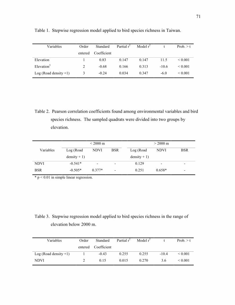
71

Table 1. Stepwise regression model applied to bird species richness in Taiwan.

Variables Order

entered

Standard

Coefficient

Partial r2 Model r2 t Prob. > t

Elevation 1 0.83 0.147 0.147 11.5 < 0.001

Elevation3 2 -0.68 0.166 0.313 -10.6 < 0.001

Log (Road density +1) 3 -0.24 0.034 0.347 -6.0 < 0.001

Table 2. Pearson correlation coefficients found among environmental variables and bird

species richness. The sampled quadrats were divided into two groups by

elevation.

< 2000 m > 2000 m

Variables Log (Road

density + 1)

NDVI BSR Log (Road

density + 1)

NDVI BSR

NDVI -0.541* - - 0.129 - -

BSR -0.505* 0.377* - 0.251 0.658* -

* p < 0.01 in simple linear regression.

Table 3. Stepwise regression model applied to bird species richness in the range of

elevation below 2000 m.

Variables Order

entered

Standard

Coefficient

Partial r2 Model r2 t Prob. > t

Log (Road density +1) 1 -0.43 0.255 0.255 -10.4 < 0.001

NDVI 2 0.15 0.015 0.270 3.6 < 0.001

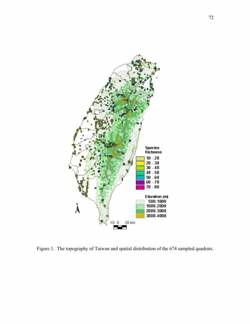
72

Figure 1. The topography of Taiwan and spatial distribution of the 674 sampled quadrats.

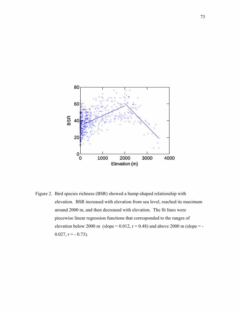
73

Figure 2. Bird species richness (BSR) showed a hump-shaped relationship with

elevation. BSR increased with elevation from sea level, reached its maximum

around 2000 m, and then decreased with elevation. The fit lines were

piecewise linear regression functions that corresponded to the ranges of

elevation below 2000 m (slope = 0.012, r = 0.48) and above 2000 m (slope = -

0.027, r = - 0.73).

0 1000 2000 3000 4000Elevation (m)

0

20

40

60

80

BS

R

0 1000 2000 3000 4000Elevation (m)

0

20

40

60

80

BS

R

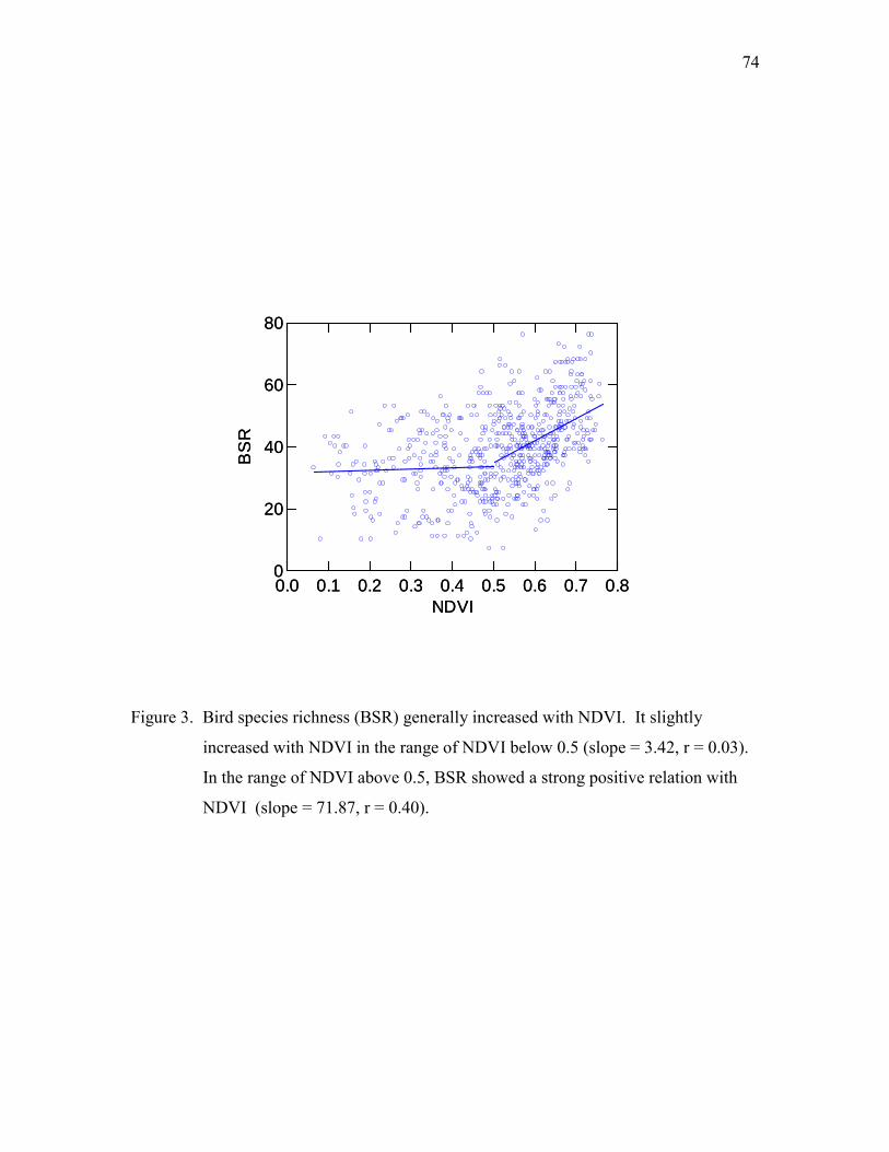
74

Figure 3. Bird species richness (BSR) generally increased with NDVI. It slightly

increased with NDVI in the range of NDVI below 0.5 (slope = 3.42, r = 0.03).

In the range of NDVI above 0.5, BSR showed a strong positive relation with

NDVI (slope = 71.87, r = 0.40).

0.0 0.1 0.2 0.3 0.4 0.5 0.6 0.7 0.8NDVI

0

20

40

60

80

BS

R

0.0 0.1 0.2 0.3 0.4 0.5 0.6 0.7 0.8NDVI

0

20

40

60

80

BS

R

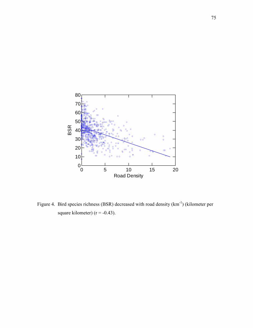
75

Figure 4. Bird species richness (BSR) decreased with road density (km-1) (kilometer per

square kilometer) (r = -0.43).

0 5 10 15 20Road Density

0

10

20

30

40

50

60

70

80

BS

R

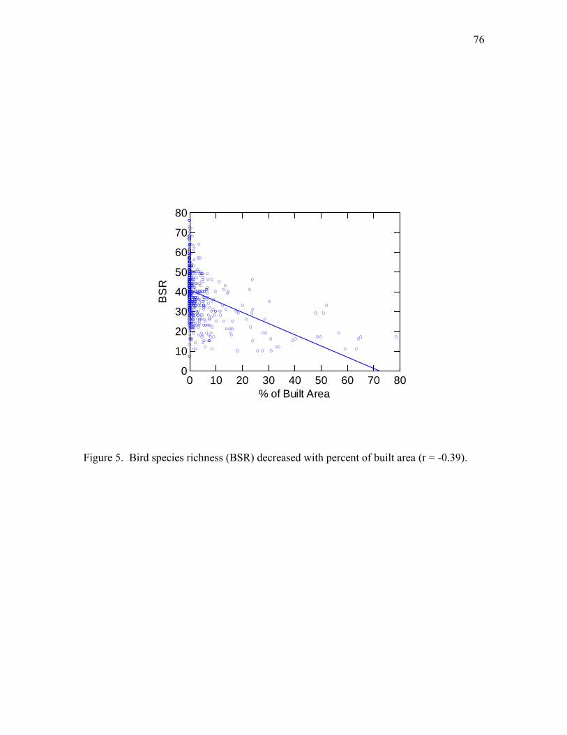
76

Figure 5. Bird species richness (BSR) decreased with percent of built area (r = -0.39).

0 10 20 30 40 50 60 70 80% of Built Area

0

10

20

30

40

50

60

70

80

BS

R

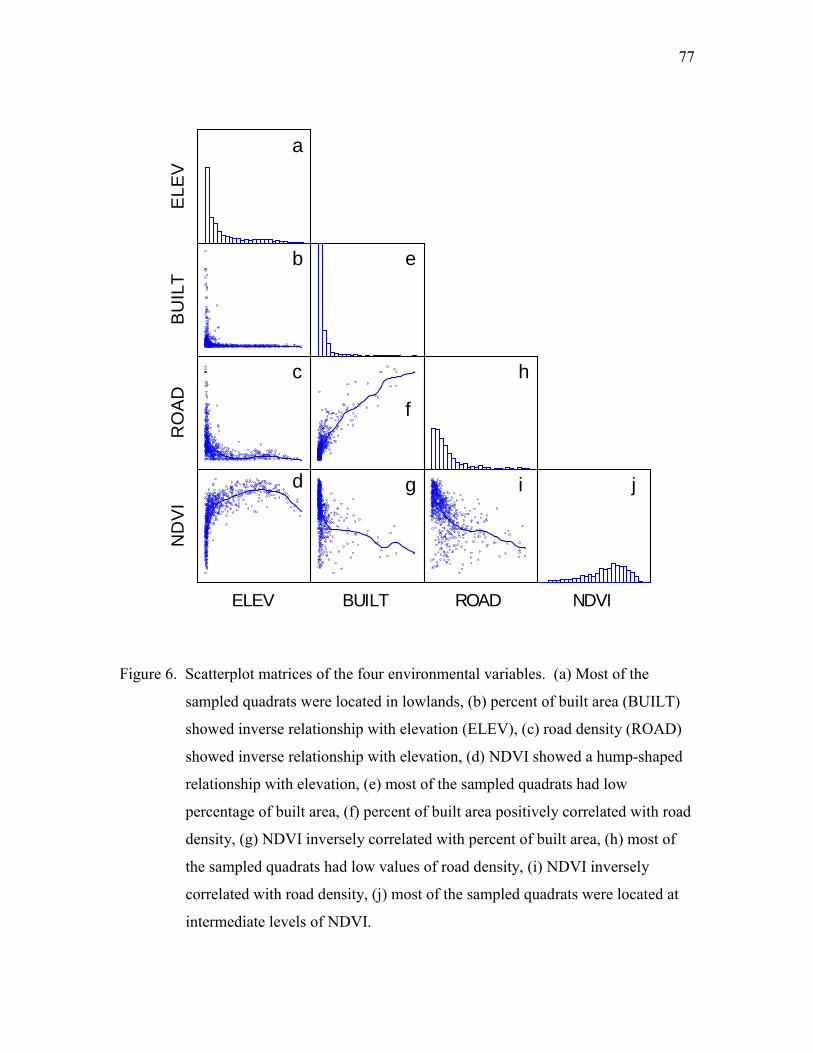
77

Figure 6. Scatterplot matrices of the four environmental variables. (a) Most of the

sampled quadrats were located in lowlands, (b) percent of built area (BUILT)

showed inverse relationship with elevation (ELEV), (c) road density (ROAD)

showed inverse relationship with elevation, (d) NDVI showed a hump-shaped

relationship with elevation, (e) most of the sampled quadrats had low

percentage of built area, (f) percent of built area positively correlated with road

density, (g) NDVI inversely correlated with percent of built area, (h) most of

the sampled quadrats had low values of road density, (i) NDVI inversely

correlated with road density, (j) most of the sampled quadrats were located at

intermediate levels of NDVI.

ELEV

BUIL

TR

OAD

ELEV

ND

VI

BUILT ROAD NDVI

a

b

c

d

e

f

g

h

i j

78

Chapter Three

Spatial Patterns of Bird Species Richness in East Asia

79

Abstract

Spatial patterns of species diversity at continental scale have been a subject of

major interest and investigation in ecology. Yet, despite of its distinct geographical

setting and large share of global biodiversity, there is lacking of literature that documents

species richness of any major taxon in East Asia (Asia east of 70º E longitude, including

Wallacea). In this study, I developed maps of bird species richness (BSR) in East Asia

by overlaying the breeding ranges of 2,406 terrestrial bird species and also studied the

relationship of BSR with primary productivity, area, isolation, topographic heterogeneity,

human population density, and historic environmental changes. Generally BSR declined

from the tropics to the arctic. However, there were two minor exceptions in Mainland

East Asia. BSR was highest around Tropic of Cancer and it fluctuated between 30º and

50º N. Islands had lower BSR than adjacent mainland areas. Normalized Difference

Vegetation Index (NDVI) showed strong and positive correlation with BSR in both

mainland areas and islands. For mainland areas, NDVI explained 65% of the BSR

variation and topographic heterogeneity explained an additional 6%. On islands, BSR

significantly correlated with island area but inversely with distance to mainland. NDVI

explained 66% of the BSR variation on islands, which island area explained an additional

13%, and distance to mainland accounted for an additional 1%. I argue that energy

availability is the primary process for the observed spatial patterns of BSR in East Asia.

However, its effect might not be remarkable on isolated regions, where area size and

degree of isolation also have significant influences on BSR. Other factors might also

affect species diversity but their influences are not as profound as energy availability,

isolation, and area.

80

Introduction

Spatial patterns of species richness are major research topics for ecologists,

systematists, and biogeographers. The most acknowledged one is that species diversity

peaks in the tropics and declines when one moves away from the equator (Stevens 1989).

Although few taxa, such as aphids (Dixon et al. 1987) and Ichneumonidae (Owen and

Owen 1974, Jazen 1981), show their highest species richness in temperate regions, most

other major taxa display a latitudinal diversity gradient (Rosenzweig 1995). This

latitudinal diversity gradient has been widely reported and suggested as one of the most

consistent ecological patterns (Gaston and Blackburn 2000).

More than 25 hypotheses have been proposed to explain the latitudinal diversity

gradient (examples in Pianka 1966, Rohde 1992, Rosenzweig 1995, Brown and Lomolino

1998). Some hypotheses are circular – assuming higher species diversity in the tropics

(Rohde 1992), which include the competition hypothesis, mutualism hypothesis, and

predation hypothesis. Some other hypotheses, such as the environmental stability

hypothesis, do not have sufficient evidence to support (Rohde 1992). Some authors

(Rohde 1992, Rosenzweig 1995, Gaston and Blackburn 2000, Rahbek and Graves 2001)

consider the most promising hypotheses are the time theory (Fisher 1960), energy

limitation theory (Hutchinson 1959, Connell and Orias 1964, Currie 1991), and area

theory (Terborgh 1973, Rosenzweig 1992, 1995). The time theory suggests that lower

latitudes are relatively free of Pleistocene glaciations and severe climatic disruptions, thus

enabling more species to persist and evolve than higher latitudes (Fischer 1960, Simpson

1964). The energy limitation theory suggests that, since the tropics usually receive higher

81

solar radiation and precipitation, they therefore have higher primary productivity which

provides wider resource base and permits more species to co-occur (Connell and Orias

1964, Currie 1991). The area theory argues that since the Earth is a sphere, the lower

latitudes have larger geographical area and this increases species richness through the

reduction of extinction rates and increase of allopatric speciation rates (Rosenzweig

1992).

Ideally, studies on the latitudinal diversity gradient should cover spatial extent

from the tropics to the arctic. Partial coverage may result in misleading patterns. For

example, Currie (1991) found bird species richness of North America (north of 25° N)

peaked around 45° N longitude. However, Blackburn and Gaston (1996) found bird

species richness of the New World peaked around the equator and monotonically

declined toward the poles. On the Earth, North America, South America, and East Asia

are the only continents that span from the tropics to the arctic. However, most studies on

latitudinal richness gradient were conducted in North and South America, with some in

Africa, Australia and Europe. Little if any literature has mapped distributional patterns of

species richness of any major taxa in East Asia (Asia east of 70°E longitude), in spite of

its large share of global biodiversity.

East Asia has at least four distinct geographical characteristics. First, there is a

chain of islands spanning from the tropics to the arctic. These islands display great

variation in size and distance to mainland. Second, tropical East Asia is mostly

composed of islands. Mainland East Asia is mainly located in the subtropical, temperate,

and arctic zones. The extensions of Eurasia in the tropical zone are all peninsulas (such

as Malay Peninsula and India Peninsula) and are isolated from the main part of Eurasia.

82

Third, East Asia has a distinct latitudinal productivity gradient. In West Asia, Africa,

Australia, North America, and South American, deserts mainly locate between 20° and

30° latitude. In East Asia, due to the blocking effect of the Tibetan Plateau, the deserts

mainly locate from 35° to 45°N latitude and the latitudinal zone between 20° and 30° N

in East Asia actually has extremely high precipitation and primary productivity (An et al.

2001). Fourth, East Asia contains half of the world’s population. Cultivation and

modification of natural vegetation have been extensive for thousands of years. All these

characteristics make East Asia a distinct site for studying spatial patterns of species

richness at the continental scale. By comparing with other continents, East Asia provides

a unique opportunity to study the processes of the latitudinal diversity gradient.

Because of their well-studied taxonomy and distribution, birds have been

frequently used in studies of species diversity at broad spatial scales. Of the total 9,702

bird species on the Earth, 2,466 species breed in East Asia and 1,906 species can only be

found in East Asia (summarized from Monroe and Sibley, 1993). The main objectives of

this study are to: (1) establish a fine-scale map of bird species richness in East Asia; (2)

investigate the relationships of species richness with area, isolation, primary productivity,

topographic heterogeneity, human population density, and historic environmental

changes.

83

Historic environment of the study area

The study area was defined as Asia between 70°E and 180°E longitude (Figure 1).

In zoogeographic classification, it included the eastern half of Palearctic Region, entire

Oriental Region, and entire Wallacea Subregion (part of Australian Region). The

Wallacea Subregion (Mayr 1944), defined as the Indonesian Islands between Wallace’s

line and Lydekker’s line, was included because of its strong affinity with the Oriental

Region. The latitudinal extent of the study area ranged from 10°S to 80°N (Lesser Sunda

Islands to Severnaya Zemlya).

The oldest fossils that have primitive characteristics of Class Aves,

Archaeopteryx, dated back to the Late Jurassic, about 150 million years ago (MYA). All

the fossil bird species in the Cretaceous (144 - 65 MYA) were toothed and most of them

became extinct at the end of the Mesozoic (65 MYA) (Feduccia 1995). After the mass

extinction, birds underwent a dramatic adaptive radiation and all modern orders of birds

were found as fossils in Palearctic Region during the ten million year period in the

Paleocene and early Eocene (55-65 MYA) (Blondel and Mourer-Chauvire 1998).

Among them, Order Passeriformes (passerines or songbirds) experienced an explosive

radiation in the Late Oligocene and Miocene (20 - 5 MYA) and now constitute nearly

60% of living bird species. All modern avian families have arisen by the Oligocene (38-

26 MYA), and all modern genera by the Miocene (26-5 MYA) (Feduccia 1995). During

the Palaeogene (65-26 MYA) the Earth’s climate was subtropical, without marked

seasonality, and forests dominated most of the Northern Hemisphere (Blondel and

Mourer-Chauvire 1998). The gradual global cooling in the Neogene (26 – 1.6 MYA)

84

resulted in the appearance of a latitudinal thermal gradient and seasonal climates in

higher latitudes.

Mountain building by tectonic movements

In the early Jurassic (about 180 MYA), the supercontinent of Pangea began to

break into two landmasses: Laurasia and Gondwanaland. At that time, India and Arabia

were part of Gondwanaland and most of the rest of present-day Asia was part of Laurasia.

During the middle Cretaceous (about 100 MYA), India broke away from Gondwanaland

and drifted northwards rapidly. In the middle Eocene (about 50 MYA), the India Plate

collided with Eurasia Plate. However, the initial collision was gentle in the Eocene, not

accompanied by any massive upheaval of the terrain. A forceful collision between the

two plates started in the early Miocene (about 26 MYA) and resulted in the uplift of the

Himalayas, Tibetan Plateau, and the N-S trending mountain ranges in Indochina

Peninsula (Whitmore 1987). Evidence showed that the Himalayas were probably over

3000 m and the Tibetan Plateau more than 1000 m above sea level at the end of middle

Miocene (about 12 MYA) (Xu 1991, Wu et al. 1991). Most of the uplift took place

during the Pleistocene (1.6 – 0.01 MYA) and is still continuing. Zhang et al. (1991)

showed that the main part of Tibetan Plateau is still rising at a mean rate of 5.8 mm/year,

with the highest rate, 10 mm/year, in the northern Himalayas.

Uplifts of the Himalayas and Tibetan Plateau caused a dramatic effect on the

climate. By their vast area and very height, the Himalayas and Tibetan Plateau changed

the paths of seasonal winds in East Asia and increased the aridity in the central part of

East Asia. In summer, the Tibetan Plateau intercepts large quantities of solar radiation.

85

As the heat rises, it draws in airs from lower altitudes (anabatic winds) and brings

moisture from India Ocean and Pacific Ocean. The moisture condenses and is

intercepted by the Himalayas and the N-S trending mountains in Indochina Peninsula,

creating monsoons, the characteristic climate pattern in East Asia. Evidence from soil

carbon isotopes suggests that by the end of Miocene (around 7 MYA) a monsoonal

climate was already in place (Quade et al. 1989). The monsoons brought extremely high

precipitation to the latitudinal zone between 20° and 30° N in East Asia, where

corresponding latitudinal zones in other continents are mostly deserts.

Around the early Pliocene (about 4 –5 MYA), the Pacific Plate started to rotate

and caused collisions with Philippine Plate and Eurasian Plate, and subsequently resulted

in the uplifts of Luzon, Taiwan, Ryukyu islands, and Japan (Teng 1990, Aubouin 1990).

Glaciation and sea-level fluctuation in the Pleistocene

During the Pleistocene (1.6 MYA to 0.01 MYA), the Earth experienced several

glacial-interglacial cycles during which glaciers advanced and retreated. Unlike North

America and Europe, great portions of northern Asia were not glaciated at all during the

Pleistocene due to low precipitation (Nilsson 1983). During the greatest glacial

maximums, the West Siberian ice sheet only reached southwards to 55º N and eastwards

to 120º E. Beyond that region, glaciation was confined to the mountain ranges in East

Siberia and Central Asia. The permafrost line, which currently lies around 48º N (Shi

1991), might have extended southwards to 30º N (Pu 1991). The glacial cycles led to

significant changes in climatic regime and vegetation in areas north of 30 º N. South of

30º N, the climates remained relatively stable, similar to what they are today; therefore

86

they served as refuges for Tertiary (65 – 1.6 MYA) taxa to survive through the glacial-

interglacial cycles (Ferguson 1993). Some authors (Adams and Woodward 1989, Latham

and Ricklefs 1993) argued that the distinct paleoenvironment of East Asia contributed to

the far greater temperate tree species richness in East Asia – three times more than forests

in eastern North America and six times more than those in Europe.

During the glacial maximums, a large volume of water was removed from the ocean

and sea levels fluctuated dramatically. The lowering of sea level by some 100 to 160 m

below present, resulted in the formation of land bridges among currently isolated

landmasses. East Asia was connected with North America through Beringia and most of

the major islands in East Asia were connected to Mainland Asia during the glacial

maximums (Voris 2000). One exception was Wallacea. While Borneo, Java, and

Sumatra were all connected to mainland Asia, the waters surrounding the islands of

Wallacea were deep enough to prevent landbridge connection. Thus, islands in Wallacea

were never connected by Pleistocene landbridges to either Southeast Asia or Australia-

New Guinea. The latest glacial period (Wisconsin Glaciation) reached its maximum

around 18 thousand years ago (KYA). By 6 KYA, the sea level in East Asia had risen to

its present level or even exceeded it by 1-7 m (Guo 1979, Wang and Wang 1980, Chen

and Liu 1996). However, the latest glaciation was relatively mild in comparison to some

earlier glacial maximums and resulted in only a 100 m drop in sea level. Many islands in

East Asia, such as Philippines, that had past land connections with Mainland Asia were

not connected during the latest glaciation (Heaney 1985).

87

Methods

Bird distribution ranges and species richness map

Breeding ranges of bird species were collected from various literature sources

published from 1975 to 2000 (64 books in total, detailed in Appendix 1). For those

species that lacked overall distribution maps in East Asia, their distribution ranges were

combined from sources that cover certain regions or countries. When there were multiple

sources for the distribution of one species, the most precisely delineated maps were used.

Pelagic birds, which primarily feed on marine food sources and usually have

nomadic distribution on land, were excluded in this study. These pelagic species

included Laridae (gulls, terns, auks), Phaethontidae (tropic birds), and Sulidae (boobies).

For taxonomic consistency, this study followed the taxonomy system of Monroe and

Sibley (1993). A total of 2,406 bird species, whose breeding ranges were within the

study area, were included. A checklist of those species and an atlas of their distribution

ranges in the study area are detailed on the website:

http://www.genglab.ucdavis.edu/ding/asianbird/

Each species’ breeding range was transcribed onto a Mercator projection map of the

study area and was digitized into GIS polygon coverage in ARC/INFO. The error of the

transcription process was controlled to be less than 100 km. The breeding ranges of the

2,406 species were overlaid to create the bird species richness layer.

88

Quadrat system

Many studies on species richness at continental scale used latitude-longitude

quadrats (such as 1°×1°, 5°×5°) as analysis units. The real land area of quadrats was

either unjustified (Currie and Paquin 1987) or included as one possible factor of the

observed spatial patterns of species richness (Currie 1991, Kerr and Packer 1997, Rahbek

and Graves 2001). There is a potential pitfall in this strategy: the area of the quadrat

correlates with latitude. Except for coastal quadrats, the area of inland quadrats at higher

latitudes is always less than those of lower latitudes. Justifying the area of latitude-

longitude quadrats before regression analyses could statistically obscure the correlation

between species richness and other factors that are dependent on latitude (e.g., primary

productivity, temperature). To bypass the confounding effect of area, I used equal-area

quadrats as the analysis unit (grain) for regression analyses. The country coverage in the

ESRI ArcWorld 1:3M data set (ESRI 1992) was transformed to Lambert-Azimuth equal-

area projection and overlaid with a 100×100 km quadrat system. Those quadrats with

land areas less than 3000 km2 were excluded. In total 3,433 quadrats met the criteria and

345 of them were on islands (Figure 2).

Environmental factors

Terrestrial ecosystem productivity was estimated by the Advanced Very High

Resolution Radiometer – Normalized Difference Vegetation Index (AVHRR-NDVI).

The AVHRR-NDVI was derived from the data collected by National Oceanic and

Atmospheric Administration (NOAA) and processed by National Aeronautics and Space

Administration (NASA). NDVI is a measure derived by dividing the difference between

89

near-infrared (0.725 – 1.1µm) and red (0.58-0.68 µm) reflectance measurements by their

sum (Tucker 1979).

NDVI = (Channel infrared - Channel red) / (Channel infrared + Channel red)

NDVI has been shown to be highly correlated with green-leaf biomass, green-leaf area,

and absorbed photosynthetically active radiation (APAR) (Curran 1980, Goward et al.

1985). The NDVI equation reproduces values in the range of –1.0 to 1.0, where

increasing positive values indicate increasing green vegetation and negative values

indicate non-vegetated surface features such as water, barren land, ice, and snow. Spatial

patterns of NDVI have been viewed as reasonable representations of net primary

productivity and vegetative growth of terrestrial ecosystems at continental and global

scales (Goward et al. 1985, Box et al. 1989, Ustin et al. 1991). The daily NDVI

composites usually contain a certain amount of cloud contamination. To minimize the

problem, researchers create monthly NDVI composites by maximum value composite

method; choosing the maximum daily NDVI value for each individual pixel location

(Holben 1986). However, during monsoon seasons, the monthly composites of East Asia

were still heavily plagued by cloud contamination. Therefore, the 144 monthly NDVI

composites of 12 years (1987-2000) were combined by the maximum value composite

method to create historic monthly NDVI composites. The NDVI data, with a resolution

of 8×8 km, were downloaded from the website (8th June 2001,

http://daac.gsfc.nasa.gov/data/dataset/AVHRR/01_Data_Products/06_Images/03_Asia/).

Landscape heterogeneity could be represented by variation in either topography or

land cover. Since there is a lack of accurate land cover map in East Asia and elevation

difference has profound influences on abiotic environment and biotic community, I used

90

elevation range of each quadrat (maximum minus minimum elevation recorded in each

quadrat) as an estimate for landscape heterogeneity. The elevation range was calculated

from the Global 30 Arc Second Elevation Data Set (GTOPO30), produced by U. S.

Geological Survey, EROS Data Center. GTOPO30 is a digital elevation model (DEM)

with a resolution of 30 arc seconds (approximately one kilometer). The DEM data set

was overlaid with the quadrat system and the elevation range within each 100×100 km

quadrat was calculated.

Population density data were obtained from ESRI ArcAtlas data set (ESRI 1996).

The data was compiled from various sources including national population censuses and

United Nation demographic yearbooks. Most of the databases were established between

1981 and 1994. The population density coverage was overlaid with the quadrat system to

calculate average population density of each quadrat.

Island area and distance to mainland were also calculated for the 345 quadrats

located on islands. Island area was directly calculated from the land/ocean coverage in

the ESRI ArcWorld 1:3M data set (ESRI 1992) that had converted into Lambert-Azimuth

equal area projection. Distance to mainland was calculated as the minimum distance

from this island to mainland at two-point equidistant projections.

Analyses

The distribution ranges of the 2,406 bird species were overlaid with the quadrat

system and the area of each species distribution in each quadrat was calculated. For each

species, if its distribution covered more than 25% land area of the quadrat, I assigned it as

‘present‘ in that quadrat, otherwise ‘absent’ was recorded. To test if the choice of cut-off

91

point significantly affected the results, I calculated the species richness of Anseriformes

and Sylviidae at cut-off points of 0%, 25%, 50%, and 100%. Results showed that species

richness at each cut-off point was highly correlated with each other (r > 0.98 for all of the

pair-wise comparisons). The 2,406 binary species distribution matrices were added to

create a layer of bird species richness in raster format.

The environmental factor data layers were all transformed to Lambert-Azimuth

equal-area projection and overlaid with the 100×100 km quadrat system. The average

NDVI (mean of the 1987-200 historic monthly NDVI), elevation range, and average

population density of each quadrat were calculated. By using multiple regression

analyses, the power of average NDVI, elevation range, and average population density in

explaining the variation of BSR were determined. For those quadrats located on islands,

island area and distance to mainland were also added into the regression analyses.

92

Results

Bird species richness

Within the 100×100 km quadrats, BSR ranged from 5 to 510 species. All the island

quadrats had lower BSR than adjacent quadrats in Mainland Asia. BSR was highest at

the base of Indochina peninsula, specifically the border zones of Myanmar adjacent to

India and China (Figure 3). It is the region where the Himalayas spread into tropical

lowland and has high topographic variation and low development pressure. These

species richness hotspots expanded from 20° to 30°N latitude, with the maximum spots

around Tropic of Cancer. Northern Siberia, Gobi Desert, Taklimakan Desert, and

Tibetan Plateau had lower BSR.

Along the latitudinal gradient, BSR generally declined from the tropics to the

arctic (Figure 4a). However, there are two noticeable exceptions on the mainland. First,

although the fitted curve of mainland BSR peaked around the equator, the quadrats that

had maximum BSR located around 25°N, instead of around the equator. Second, BSR

fluctuated in Mainland Asia from 30°N to 50°N. BSR rapidly decreased from 25°N to

40°N and increased again from 40°N to 50°N.

Area

Within the extent of this study, mainland made 93% of total land area (Figure 4b).

The southernmost point of Mainland Asia is located at 2°N. Within the study area, only

1% of Mainland East Asia is located south of 10°N, and only 15% were within the

tropical zone (south of Tropic of Cancer). Most of the mainland East Asia is located in

93

subtropical, temperate, and arctic zones. Islands extended from 10°S to 80°N within the

study area. However, 80% of island area is located within tropical zone and 73%

between 10°S and 10°N.

On mainland East Asia, BSR did not correspond closely with land area along the

latitudinal gradient (Figure 4). In order to test if land area correlated with BSR along the

latitudinal gradient, Mainland Asia was divided into equal-range latitudinal bands at 1°,

5°, 10°, and 20° and the land area and BSR of each band were calculated respectively.

Results showed BSR did not have any significant correlation with land area (Table 1).

For the 5° and 20° bands, land area was independent to BSR. For the 10° bands, land

area negatively correlated with BSR and only explained 4% of the variation in BSR.

On island quadrats, however, land area correlated well with BSR. After both log

transformed, BSR of island quadrats significantly correlated with island area in a simple

linear regression analysis (intercept = 2.19, slope = 0.26, r2 = 0.39, p<0.001 for both

coefficients). This species-area relationship expressed in the power model is:

BSR = 2.19·Area0.26

The results suggest the effect of land area is only significant on island BSR, not on the

mainland.

Primary productivity

There were high spatial and temporal variations among monthly NDVI (Figure 5).

In tropical Asia, NDVI remained at a high level all year round. However, in temperate

and arctic zones, NDVI had great seasonal variations. Tibetan Plateau, Gobi Desert, and

Taklimakan Desert had low NDVI all year round. Average NDVI was highest in tropical

94

islands (e.g., Borneo, Sumatra, and Sulawesi) and mountain ranges of the Indochina

Peninsula and was lowest in Taklimakan Desert, Gobi Desert, and Northern Siberia

(Figure 6).

Average NDVI significantly and positively correlated with BSR (slope = 380.0, r2

= 0.59, t = 70.4, p < 0.001). After separating the quadrats into two groups (mainland and

islands), NDVI explained 65% of the variation in mainland BSR (slope = 430.67, t =

76.4, p < 0.001) (Figure 7a) but only 30% of the variation in island BSR (slope = 423.71,

t = 12.1, p < 0.001) (Figure 7b) in simple linear regression analyses.

BSR mainland = -0.58 + 430.67·NDVI

BSR island = -65.37 + 423.71·NDVI

To test if the slopes and intercepts of both regression equations were significantly

different, the significance levels of coefficients of following regression model were

estimated.

BSR = β0 + β1 · X + β2 · NDVI + β3 · X · NDVI

X = 0, if on mainland quadrats,

X = 1, if on island quadrats.

The slope of the mainland BSR was not significantly higher than island BSR (Hnull : β3 =

0, t = -0.28, p = 0.78). However, the intercept of mainland BSR was significantly higher

than island BSR (Hnull : β1 = 0, t = 3.82, p < 0.001 ). These results confirm that islands

have lower BSR than on the mainland and suggest that the increments of primary

productivity on BSR are similar on mainland and islands.

95

Topographic heterogeneity

Elevation range was high in the Himalayas, Tienshan, Kunlunshan, and some

islands in Western Pacific Ocean (such as Java, Sumatra, Taiwan, and Sulawesi) (Figure

8). Elevation range positively correlated with BSR (slope = 0.0244, t = 16.9, p < 0.001)

but only explained small proportion of variation in BSR (r2 = 0.08). After separating the

quadrats into two groups (mainland and islands), elevation range still positively

correlated with BSR of mainland quadrats (slope = 0.0246, t =17.0, p < 0.001, r2 = 0.09)

but did not significantly correlate with BSR of island quadrats (slope = 0.0063, t = 1.0, p

= 0.32).

Population density

Human populations were unevenly distributed over East Asia (Figure 9). Some

areas were densely populated (density > 1000 persons/km2), while some vast areas were

almost unpopulated (e.g., Tibetan Plateau, Taklimakan Desert) (density < 1 person/km2).

In a simple linear regression analysis, population density positively correlated with BSR

(slope = 0.162, t = 11.1, p < 0.001) but only explained 3% of the variation in BSR. After

separating the quadrats into two groups (mainland and islands), population density still

positively correlated with BSR of mainland quadrats (slope = 0.231, t =11.8, p < 0.001, r2

= 0.04) but did not significantly correlate with BSR of island quadrats (slope = 0.032, t =

0.49, p = 0.63).

96

Multiple regressions

Stepwise forward multiple regression (criteria for inclusion and exclusion, p <

0.05) was applied to evaluate the effects of NDVI, elevation range, and population density

on mainland BSR. NDVI explained 65.4% of variance in mainland BSR (p < 0.001),

Elevation range explained an additional 5.7% (p < 0.001), and population density only

explained an additional 0.1% (p = 0.007) (Table 2). Primary productivity was the best

variable in explaining the variation of mainland BSR. The standard coefficients for NDVI,

elevation range, and population density were 0.802, 0.237 and –0.028 respectively.

Results suggest mainland BSR increases with primary productivity and topographic

heterogeneity but decreases with population density. Notably, population density

positively correlated with mainland BSR in a simple linear regression but negatively

correlated with the residuals of mainland BSR once the effects of NDVI and elevation

range had been justified.

For island BSR, island area and distance to mainland were added into the multiple

regression analysis. All the variables were log-transformed to fit the normality assumption

of regression analysis and fix the problem of inconsistent variance of the errors. NDVI

explained 66.2% of variance in island BSR (p < 0.001), island area explained an additional

14.9% (p < 0.001), and distance to mainland explained an additional 0.8% (p < 0.001)

(Table 3). Elevation range and population density were excluded in the final model

because of their insignificant contribution to the model. The standard coefficients for

NDVI, island area, and distance to mainland were 0.718, 0.401 and –0.089 respectively.

These results suggest primary productivity is the most influential variable in explaining the

97

variation of island BSR. Generally, island BSR increases with primary productivity and

island area but decreases with distance to mainland.

98

Discussion

Earlier ecologists (e.g., MacArthur and Connell 1966) believed that the latitudinal

diversity gradient should have a general explanation since it is a widespread and

consistent ecological pattern. For years, more than 25 hypotheses have been proposed to

explain the latitudinal diversity gradient. There are at least three reasons that might

answer why there are so many competing hypotheses in explaining latitudinal diversity

gradient. First, those hypotheses are not mutually exclusive. Many of the proposed

factors could have operated together, either sequentially or concurrently, to affect current

latitudinal patterns of species richness (Brown and Lomolino 1998, Whittaker et al.

2001). Second, as wide as the spatial extent of the latitudinal diversity gradient is,

ecologists have to rely on comparison studies that do not provide clear cause-effect

relationships. Third, most investigators have focused on testing only one single

hypothesis, instead of testing multiple processes simultaneously.

Most ecologists now are convinced that species diversity is governed by multiple

processes that function at various spatial and temporal scales. Most of the arguments

focus on which ones are primary processes of species diversity and which are secondary.

Brown and Lomolimo (1998) argued the primary hypotheses should relate to some

abiotic characteristics of the Earth and those hypotheses (e.g., inter-specific competition

begets species diversity) which purely rely on biological characteristics and make no

direct reference to the Earth’s abiotic template should be secondary. Here I discuss three

theories that are often considered as primary causes of the latitudinal diversity gradient:

the time theory, energy limitation theory, and area theory. In addition, the spatial

heterogeneity theory and the effect of human population density are also discussed.

99

Time theory

Without dramatic disturbance, the total number of species in biotic communities

generally increases with time. The time theory argues that higher latitudes have younger

communities than lower latitudes because of the Pleistocene glaciations and severe

climatic disruptions in the past. The time theory can be split into ecological time and

evolutionary time theories (Pianka 1966). The ecological time theory, dealing with a

shorter span of time, proposes that the lower richness in higher latitudes is a consequence

of the shorter period available for species to colonize from lower latitudes. The

evolutionary time theory proposes that the lower richness at higher latitudes is because

species have not had enough time to diversify, focusing on speciation rather than

colonization.

If the time theory is correct, the most glaciated areas should have the lowest species

richness. That is, higher latitudes and altitudes are expected to have lower species

richness. In this study, within the band between 50º and 80º N, BSR declined

monotonically with latitude, which is consistent with the prediction of the time theory.

However, within the band between 35º and 80º N, a hump-shaped relationship between

BSR and latitude was observed. BSR was higher in Tienshan and those mountain ranges

in Southern Siberia and Northern Mongolia. These mountain ranges were heavily

glaciated in the Pleistocene and even served as centers of glaciation during earlier glacial

stages (Nilsson 1983). These mountain ranges should have lower BSR than adjacent

regions, as Tibetan Plateau did. Similar patterns have been also observed in Europe and

temperate North America. The bird species richness has been reported highest at mid-

100

latitudes within Europe (Mönkkönen 1994, Gregory et al. 1998) and Rocky Mountains

and Sierra Nevada within North America (Simpson 1964, Cook 1969), all of which were

heavily glaciated in the Pleistocene.

It is certainly true that historical factors can affect contemporary species diversity.

However, these results suggest that the effects of historical glaciation are either not long

lasting or insignificant for birds in East Asia. Birds are known as good migrators and

many birds have the greatest capability for long distance dispersal. Their strong dispersal

ability should, on average, enable birds to colonize newly available habitats within a

relatively short temporal scale. The impacts of historic disturbances in the Pleistocene

might therefore not be important for contemporary bird species richness. The observed

spatial patterns of BSR in East Asia should be regulated primarily by ecological

processes (e.g., energy availability, spatial heterogeneity) that function on a relatively

short temporal scale.

Energy limitation theory

Most living organisms on Earth either directly or indirectly depend on the energy

radiated from the sun. The energy fixed by plants establishes the upper limit for a

community to support organisms and species. The energy limitation theory proposes that

higher energy availability in a given area can support more species because, in general,

species can be more specialized and still be able to maintain sufficiently large population

sizes to avoid extinction (MacArthur 1972). At local scales, many studies however show

evidence against the energy limitation theory; the relationship between species richness

and available energy is often found to be hump-shaped (Tilman 1988, Rosenzweig

101

1995). However, at continental scale, primary productivity and species richness of

various plant and animal groups have shown a positive monotonic relationship (Currie

and Paquin 1987, Adams and Woodward 1989, Currie1991, Blackburn and Gaston 1996,

Gaston 2000). My results show a similar pattern. Overall, BSR positively and

monotonically correlates with primary productivity in East Asia. This monotonic

relationship is especially significant in Mainland East Asia, where BSR corresponded

closely to NDVI.

This relationship between energy and BSR was not strong on islands. All the islands

had fewer bird species than adjacent regions in Mainland Asia, even though the islands

had similar or higher primary productivity and topographic heterogeneity. Some paired

examples are Southern Japan to Korea, Taiwan to Southern China, Sri Lanka to Southern

India, and Borneo to Malay Peninsula. This impoverishment of island biota can be

attributed to the isolated nature of islands. The water barriers surrounding islands reduce

immigration possibilities of organisms and make species on islands more vulnerable to

regional extinction. The isolation effect explains why the highest BSR is located on the

subtropical mountains of the Indochina Peninsula, instead of on the tropical islands,

which has the highest primary productivity. Among the tropical islands, it is also

significant that larger islands tend to have more bird species than smaller islands, even

though they have similar levels of primary productivity.

Nevertheless, primary productivity is an important variable in explaining BSR in

East Asia. The results suggest energy availability should be the most important process

in regulating BSR in East Asia. Other factors, though they explained in some detail

spatial patterns of BSR, can not explain the overall pattern observed.

102

Area theory

The area-species relationship has been suggested as one of the few rules in

community ecology. Most world maps are shown in Mercator projection that gives a

false impression that Earth has more land area at higher latitudes. However the Earth

actually has more land area at lower latitudes. The area theory extends the area-species

relationship and posits that the larger area in lower latitudes increases species richness

through reducing the extinction rate of species (Rosenzweig 1992) and increasing the

chances for allopatric speciation (Terborgh 1973).

As mentioned before, East Asia has one distinct geographical characteristic: the

temperate and subtropical regions have far larger areas than tropical regions. If the area

theory is correct, BSR should correspond closely to geographical area along the

latitudinal gradient and the vast area in the temperate East Asia should have very high

BSR. My results contradict the prediction of the area theory. BSR was higher in

Tropical East Asia, where has smaller area but higher primary productivity. The higher

BSR observed in Tropical East Asia should be a sequence of higher primary productivity

there, rather than the smaller geographical area. The area theory is rejected in this study

because of its inability to explain the latitudinal BSR gradient in East Asia.

One might argue that, overall, the Earth still has larger area and higher species

diversity in the tropical zone. However, the terrestrial tropical ecosystem on the Earth is

separated into three isolated regions: America, Africa, and Asia-Australia. Each is far

away from others and the three regions share few common bird species. The vast area

103

and rich avifauna on the other two tropical regions therefore have little or no effect on

reducing extinction rate or increasing colonization rate of bird species in tropical Asia.

Nevertheless, at regional scale, area showed a strong correlation with BSR for

isolated habitats. Larger islands tended to have more bird species, which was consistent

with the prediction of the island biogeography theory (MacArthur and Wilson 1967).

This relationship still held after the effect of primary productivity (NDVI) was adjusted.

Although area alone can not explain the overall latitudinal diversity pattern observed in

East Asia, it can play an important role for species diversity of isolated areas at regional

scale.

Spatial heterogeneity

Spatial heterogeneity theory posits that more diverse physical and biotic habitat

structure permits finer subdivision of limiting resources and hence promotes greater

specialization of species. For terrestrial birds, the heterogeneity of habitat can be split

into structural complexity of vegetation and landscape heterogeneity. MacArthur and his

associates (MacArthur and MacArthur 1961, MacArthur et al. 1966) studied bird species

richness and habitat characteristics in different habitats of North America and found that

BSR was highly correlated with foliage height diversity. Since then, structural

complexity of vegetation has been referred to as one possible cause of the latitudinal

species gradient (e.g., Pianka 1966). However, structural complexity of vegetation might

not be a direct cause of species diversity but a property caused by others factors that also

affect species diversity. Factors like historic perturbation and productivity might affect

both species diversity and structural complexity of vegetation. In addition, structural

104

complexity of vegetation itself is a product of plants. It might be a consequence of

species diversity rather than a cause. Clearly, structural complexity of vegetation is not

an adequate explanation for species diversity along a latitudinal gradient.

Landscape heterogeneity has been widely used as estimate of spatial heterogeneity at

regional and continental scales. At these broader scales, more habitats (vegetation type,

land cover, or ecosystem) will enable more species that specialized in certain habitats to

occur together and thus increase species diversity. Landscape heterogeneity has been

found to be one important factor of species diversity at broader spatial scales. It also has

been found to correlate with island area and is often used as one explanatory mechanism

of the area-species relationship. However, landscape heterogeneity does not have a

consistent relationship with latitude. Higher latitudes do not necessarily have lower

landscape heterogeneity than lower latitudes. Therefore, landscape heterogeneity is often

used as a secondary or independent process of species diversity on the latitudinal

gradient. In this study, I used topographic heterogeneity as estimate of landscape

heterogeneity. Although it only explained a small amount of variation, it significantly

correlated with BSR. In addition, topographic heterogeneity was independent of primary

productivity in this study. Its explanatory power was not weakened after the effect of

primary productivity was statistically controlled.

Population density

Higher human population densities usually cause more anthropogenic

perturbations and could reduce species diversity of natural ecosystems. Since East Asia

contains half of the world population and has been extensively colonized for thousands of

105

years, I included population density as a possible factor of BSR. Simple linear regression

revealed population positively correlated with BSR. However, the positive but weak

correlation does not necessarily imply that population density begets species diversity. It

might reflect correlation among human population density, BSR, and other factors, such

as primary productivity. For example, human beings avoid dwelling in low productivity

areas where conditions are not suitable for agricultural cultivation. After the effect of

primary productivity was justified, population density did show a significantly negative

relationship with BSR.

In conclusion, I argue that bird species richness in East Asia is primarily governed

by energy availability. Primary productivity establishes the upper limits of habitats’

capacity to contain species and the number of bird species. The hump-shaped

relationship between productivity and species diversity was not observed at continental

scale. However, in isolated areas (such as islands and peninsulas), birds might not able to

reach the richness limits set up by primary productivity. In that case, degree of isolation

and area size might also be influential in determining species diversity. Other factors,

such as spatial heterogeneity, biotic interactions, and perturbations, may also affect

species diversity. However, their influences are secondary and not strong as energy

availability, isolation, and area size.

106

Literature Cited

Aubouin J. 1990. The west Pacific geodynamic model. Tectonophysics 183:1-7.

Adams, J. M. and F. I. Woodward. 1989. Patterns in tree species richness as a test of the

glacial extinction hypothesis. Nature 339:699-701.

An, Z.,J. E. Kutzbach, W. L. Prell, L. Warren, and S. C. Porter. 2001. Evolution of Asian

monsoons and phased uplift of the Himalaya-Tibetan plateau since Late Miocene

times. Nature 411:62-66.

Blackburn, T. M. and K. J. Gaston. 1996. Spatial patterns in the species richness of birds

in the New World. Ecography 19:369-176.

Blondel, J. and C. Mourer-Chauvire 1998. Evolution and history of the western

Palaearctic avifauna. Trends in Ecology & Evolution 13: 488-492.

Box, E. O., B. N. Holben, V. Kalb. 1989. Accuracy of the AVHRR vegetatton index as a

predictor of biomass, primary productivity and net CO2 flux. Vegetatio 80:71-89.

Brown, J. H. and M. V. Lomolino. 1998. Biogeography: second edition. Sinauer,

Sunderland, MA, USA.

Chen, Y. G. and T. K. Liu. 1996. Sea Level Changes in the Last Several Thousand Years,

Penghu Islands, Taiwan Strait. Quaternary research 45:254-262.

Connell, J. H. and E. Orias. 1964. The ecological regulation of species diversity.

American Naturalist 98:399-414.

Cook, R. E. 1969. Variation of species density of Northern American Birds. Systematic

Zoology 18:63-84.

107

Curran, P. J. 1980. Multi-spectral remote sensing of vegetation amount. Progress in

Physical Geography 4:315-321.

Currie, D. J. 1991. Energy and large-scale patterns of animal- and plant- species richness.

American Naturalist 137:27-49

Currie, D. J. and V. Paquin. 1987. Large-Scale Biogeographical Patterns of Species

Richness of Trees. Nature 329:326-327

Dixon, A. F. G., P. Kindlmann, J. Leps, and J. Holman. 1987. Why there are so few

species of aphids, especially in the tropics. American Naturalist 129:580-592.

ESRI (Environmental System Research Institute). 1992. ArcWorld 1:3M. CD-ROMs.

Redlands, USA.

ESRI (Environmental System Research Institute). 1996. ArcAtlas: Our Earth. CD-ROMs.

Redlands, USA.

Feduccia, A. 1995. Explosive evolution in Tertiary birds and mammals. Science 267:637-

638.

Ferguson, D. K. 1993. The impact of late Cenozoic environmental changes in East Asia

on the distribution of terrestrial plants and animals. In N. G. Jablonski (ed.)

Evolving landscapes and evolving biota of East Asia since the Mid-Tertiary.

University of Hongkong, Hongkong, China.

Fischer, A. G. 1960. Latitudinal variations in organic diversity. Evolution 14:64-81.

Gaston, K. J.. 2000. Global patterns in biodiversity. Nature 405:220-227.

Gaston, K. J. and T. M. Blackburn. 2000. Pattern and process in macroecology.

Blackwell, Oxford, UK.

108

Gregory, R. D., J. J. D. Greenwood, and E. J. M. Hagemeijer. 1998. The EBCC atlas of

European breeding birds: a contribution to science and conservation. Biologia E

Conservazione Della Fauna 102:38-49.

Goward, S. N., C. J. Tucker, and D. G. Dye. 1985. North American vegetation patterns

observed with the Nimbus-7 Advanced Very High Resolution Radiometer.

Vegetatio 64:3-14.

Guo, X. 1979. Sea level changes since Late Pleistocene in China. Scientia Geologica

Sinica 1979:330-341.

Hagemeijer, W. J. M. and M. J. Blair. 1997. The EBCC atlas of European breeding birds

: their distribution and abundance. T & A D Poyser, London, UK.

Heaney, L. R. 1985. Zoogeographic evidence for middle and late Pleistocene land bridges

to the Philippines Islands. Modern Quaternary Research in Southeast Asia 9:127-

143.

Holben, B. N. 1986. Characteristics of maximum-value composite images from temporal

AVHRR data. International Journal of Remote Sensing 11:1417-1434.

Hutchinson, G. E. 1959. Homage to Santa Rosalia, or why are there so many kinds of

animals? American Naturalist 93:145-159.

Jazen, D. H. 1981. The peak of North American Ichneumonid speces richness lies

between 38° and 42°N. Ecology 62:532-537.

Kerr, J. T. and L. Packer. 1997. Habitat heterogeneity as a determinant of mammal

species richness in high-energy regions. Nature 385:252-254.

Latham, R. E. and R. E. Ricklefs. 1993. Continental comparisons of temperate-zone tree

species diversity. in: Ricklefs, R. E. and Schluter, D. (eds.) Species diversity in

109

ecological communities: historical and geographical perspectives. University of

Chicago Press, pp. 294-314. Chicago, USA.

MacArthur, R. H. 1972. Geographical Ecology: patterns in the distribution of species.

Harper & Row, New York, USA.

MacArthur, R. H. and J. H. Connell. 1966. The biology of populations. Wiley, New York,

USA.

MacArthur, R. H. and J. W. MacArthur. 1961. On bird species diversity. Ecology 42:594-

598.

MacArthur, R. H., H. Recher, and M. Cody. 1966. On the relation between habitat

selection and species diversity. American Naturalist 100:319-332.

MacArthur, R. H. and E. O. Wilson. 1967. The theory of island biogeography. Princeton

University Press, Princeton, USA.

Mayr, E. 1944. Wallace’s line in the light of recent zoogeographic studies. Q. Rev. Biol.

19:1-14.

Mönkkönen, M. 1994. Diversity patterns in Palaearctic and Nearctic forest bird

assemblages. Journal of Biogeography 21:185-195.

Monroe, B. L. and C. G. Sibley. 1993. A World Checklist of Birds. Yale University Press.

New Heaven, USA.

Nilsson, T. 1983. The Pleistocene: geology and life in the Quaternary ice. Reidel.

Dordrecht, Holland.

Owen, D. F. and J. Owen. 1974. Species diversity in temperate and tropical

Ichneumonidae. Nature 249:583-584.

110

Pianka, E. R. 1966. Latitudinal gradients in species diversity: a review of the concepts.

American Naturalist 100:33-46.

Pu, Q. 1991. Quaternary glaciers in China. pp. 240-273 in Zhang, Z. (ed.) The

Quaternary of China. China Ocean Press, Beijing, China.

Quade, J., T. E. Cerling, and J. R. Bowman. 1989. Development of Asian monsoon

revealed by marked ecological shift during the latest Miocene in Northern

Pakistan. Nature 342:1163-1166.

Rahbek, C. and G. R. Graves. 2001. Multiscale assessment of patterns of avian species

richness. Proceedings of the National Academy of Sciences of the United States of

America 98:4534-4539.

Rohde, K. 1992. Latitudinal gradients in species diversity: the search for the primary

cause. Oikos 65:514-527.

Rosenzweig, M. L. 1992. Species diversity gradients: we know more and less than we

thought. Journal of Mammalogy 73:715-730.

Rosenzweig, M. L. 1995. Species diversity in space and time. Cambridge University

Press. Cambridge, UK.

Shi, Y. 1991. Glaciers and glacial geomorphology in China. pp. 16-27 in Liu, T. (ed.)

Quaternary geology and environment in China. Science Press. Beijing, China.

Simpson, G. G. 1964. Species density of North American recent mammals. Systematic

Zoology 13:57-73.

Stevens, G. C. 1989. The latitudinal gradient in geographical range: how so many species

co-exist in the tropics. American Naturalist 133:240-256.

111

Teng, L. S. 1990. Geotectonic evolution of late Cenozoic arc-continent collision in

Taiwan. Tectonophysics 183:57-76.

Terborgh, J. 1973. On the notion of favourableness in plant ecology. American Naturalist

107:481-501.

Tilman, D. 1988. Plant strategies and the dynamics and structure of plant communities.

Princeton University Press. Princeton, USA.

Tucker, C. J. 1979. Red and photographic infrared linear combinations for monitoring

vegetation. Remote Sensing of Environment 8:127-150.

Ustin, S. L., C. A. Wessman, B. Curtiss, E. Kasischke, J. Way, V. C. Vanderbilt. 1991.

Oppertunities for using the EOS imaging spectrometers and synthetic aperture

radar in ecological models. Ecology 72:1934-1945.

Voris, H. K. 2000. Maps of Pleistocene sea level in Southeast Asia: shorelines, river

systems and time duration. Journal of Biogeography 27:1153-1167.

Wallace, A. R. 1876. The geographical distribution of animals. Macmillan. London, UK.

Wang, J. and P. Wang. 1980. Relationship between sea-level changes and climatic

fluctuations in East China since Late Pleistocene. Acta Geologica Sinica 35:299-

312.

Whitmore, T. C. 1987. Biogeographical evolution of the Malay Archipelago. Clarendon

Press. Oxford, UK.

Whittaker, R. J., K. J. Willis, and R. Field. 2001. Scale and species richness: towards a

general hierarchical theory of species diversity. Journal of Biogeography 28:453-

470.

112

Wu, X., F. Wang, Z. An, F. Qian, Y. Lu, and X. Zhang. 1991. Episodic uplifts of

Qinghai-Xizang Plateau and the corresponding altitudes during the late Cenozoic.

Page 393 in Abstracts XIII international Congress International Union for

Quaternary Research, Beijing, China.

Xu, Q. 1991. The first appearance of Himalayas and its relation to global climatic events.

Pages 8-10 in Abstract of Third International Conference on the

paleoenvironment of East Asia. Kunming, China.

Zhang, Q., Y. Zhou, X. Lu, and Q. Xu. 1991. On the present uplift speed of Tibetan

Plateau. Page 423 in Abstracts XIII international Congress International Union

for Quaternary Research, Beijing, China.

113

Table 1. Regression analyses at various scales showed that land area did not significantly

correlate with BSR along the latitudinal gradient in Mainland East Asia. Land

area of and the number of bird species that distributed within each 5º, 10º, 20º

latitudinal band in Mainland East Asia were calculated and log transformed to fit

the power model, log(BSR) = c + z · log(Area).

Scale n z r2 t Prob. for z > 0

5º band 15 0.005 0.00 0.028 0.98

10º band 7 -0.108 0.04 -0.506 0.64

20º band 4 -0.052 0.00 0.067 0.95

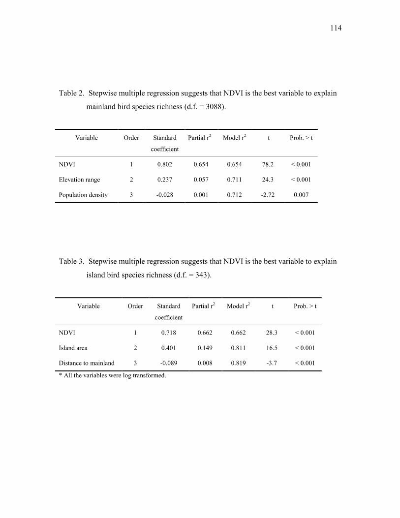
114

Table 2. Stepwise multiple regression suggests that NDVI is the best variable to explain

mainland bird species richness (d.f. = 3088).

Variable Order Standard

coefficient

Partial r2 Model r2 t Prob. > t

NDVI 1 0.802 0.654 0.654 78.2 < 0.001

Elevation range 2 0.237 0.057 0.711 24.3 < 0.001

Population density 3 -0.028 0.001 0.712 -2.72 0.007

Table 3. Stepwise multiple regression suggests that NDVI is the best variable to explain

island bird species richness (d.f. = 343).

Variable Order Standard

coefficient

Partial r2 Model r2 t Prob. > t

NDVI 1 0.718 0.662 0.662 28.3 < 0.001

Island area 2 0.401 0.149 0.811 16.5 < 0.001

Distance to mainland 3 -0.089 0.008 0.819 -3.7 < 0.001

* All the variables were log transformed.

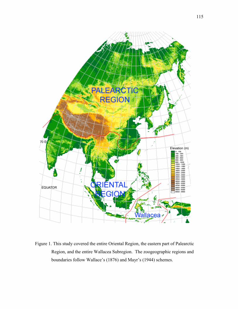
115

Figure 1. This study covered the entire Oriental Region, the eastern part of Palearctic

Region, and the entire Wallacea Subregion. The zoogeographic regions and

boundaries follow Wallace’s (1876) and Mayr’s (1944) schemes.

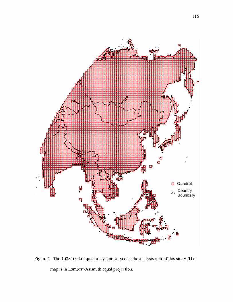
116

Figure 2. The 100×100 km quadrat system served as the analysis unit of this study. The

map is in Lambert-Azimuth equal projection.

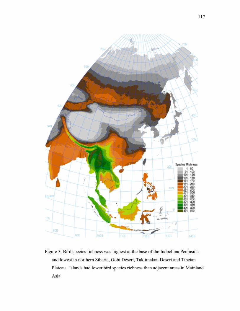
117

Figure 3. Bird species richness was highest at the base of the Indochina Peninsula

and lowest in northern Siberia, Gobi Desert, Taklimakan Desert and Tibetan

Plateau. Islands had lower bird species richness than adjacent areas in Mainland

Asia.

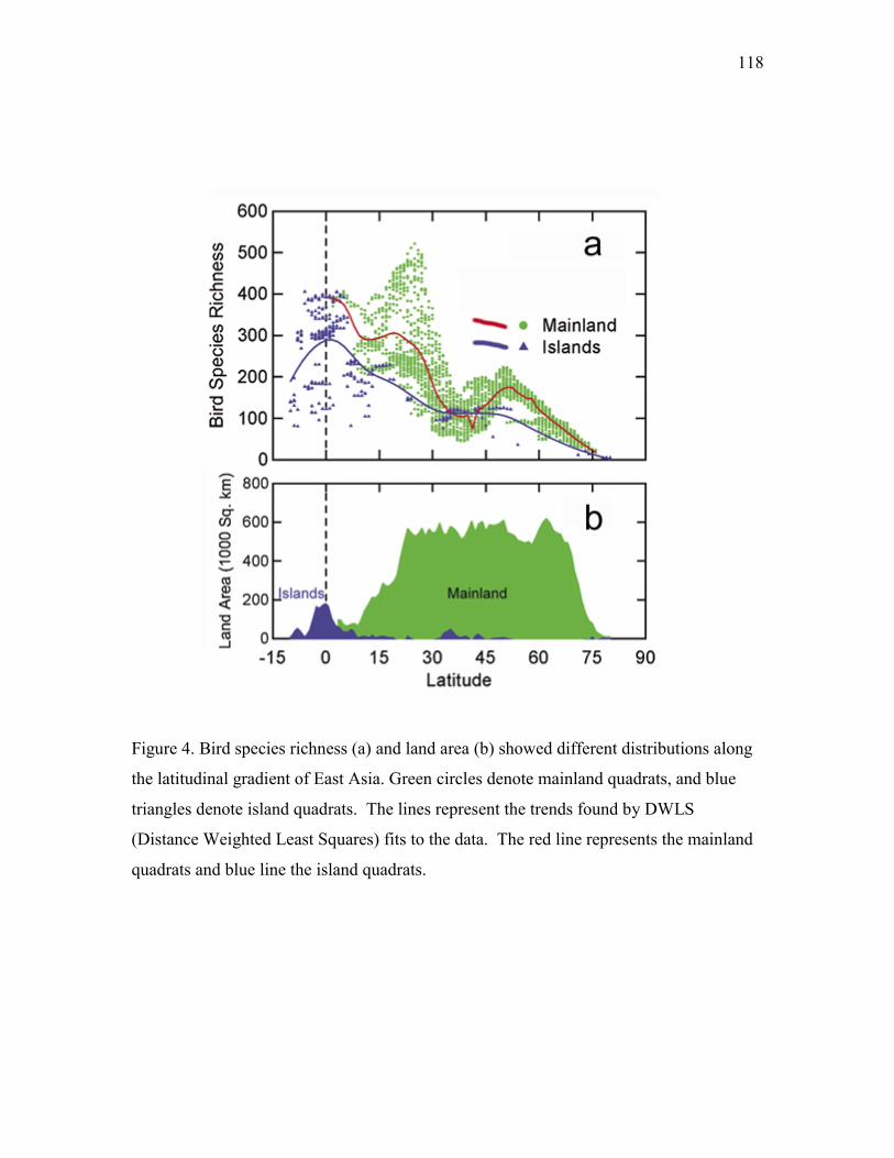
118

Figure 4. Bird species richness (a) and land area (b) showed different distributions along

the latitudinal gradient of East Asia. Green circles denote mainland quadrats, and blue

triangles denote island quadrats. The lines represent the trends found by DWLS

(Distance Weighted Least Squares) fits to the data. The red line represents the mainland

quadrats and blue line the island quadrats.

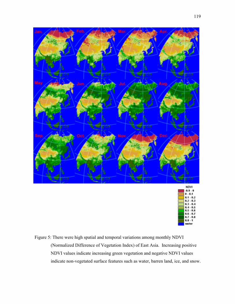
119

Figure 5: There were high spatial and temporal variations among monthly NDVI

(Normalized Difference of Vegetation Index) of East Asia. Increasing positive

NDVI values indicate increasing green vegetation and negative NDVI values

indicate non-vegetated surface features such as water, barren land, ice, and snow.

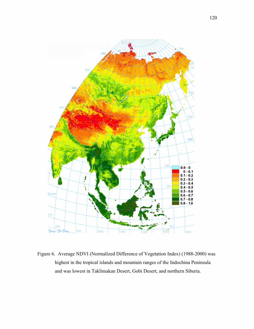
120

Figure 6. Average NDVI (Normalized Difference of Vegetation Index) (1988-2000) was

highest in the tropical islands and mountain ranges of the Indochina Peninsula

and was lowest in Taklimakan Desert, Gobi Desert, and northern Siberia.

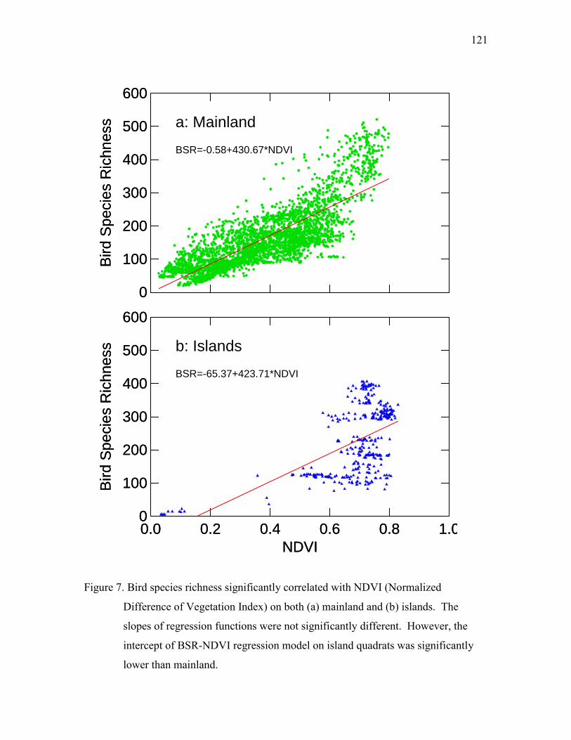
121

Figure 7. Bird species richness significantly correlated with NDVI (Normalized

Difference of Vegetation Index) on both (a) mainland and (b) islands. The

slopes of regression functions were not significantly different. However, the

intercept of BSR-NDVI regression model on island quadrats was significantly

lower than mainland.

0.0 0.2 0.4 0.6 0.8 1.0NDVI

0

100

200

300

400

500

600

Bird

Spe

cies

Ric

hnes

s

0.0 0.2 0.4 0.6 0.8 1.0NDVI

0

100

200

300

400

500

600

Bird

Spe

cies

Ric

hnes

s

0

100

200

300

400

500

600Bi

rd S

peci

es R

ichn

ess

0

100

200

300

400

500

600Bi

rd S

peci

es R

ichn

ess a: Mainland

b: Islands

BSR=-0.58+430.67*NDVI

BSR=-65.37+423.71*NDVI

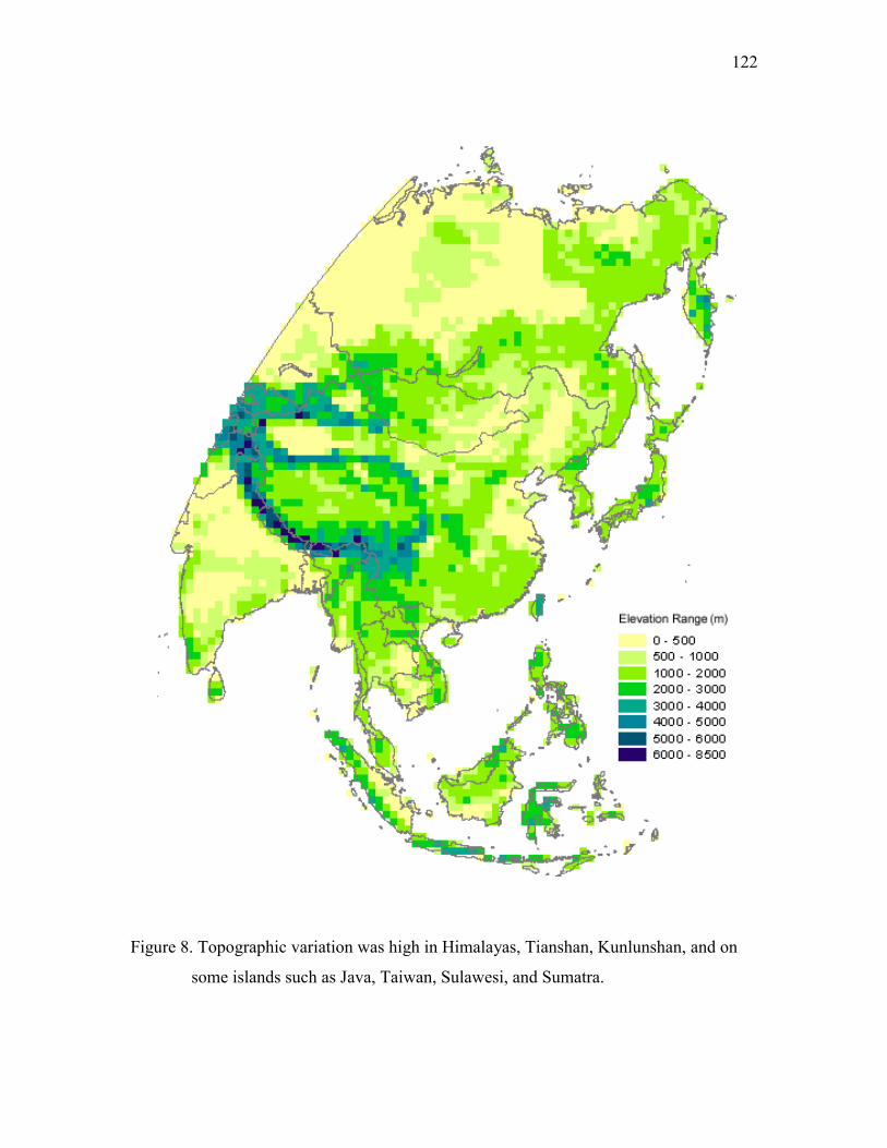
122

Figure 8. Topographic variation was high in Himalayas, Tianshan, Kunlunshan, and on

some islands such as Java, Taiwan, Sulawesi, and Sumatra.

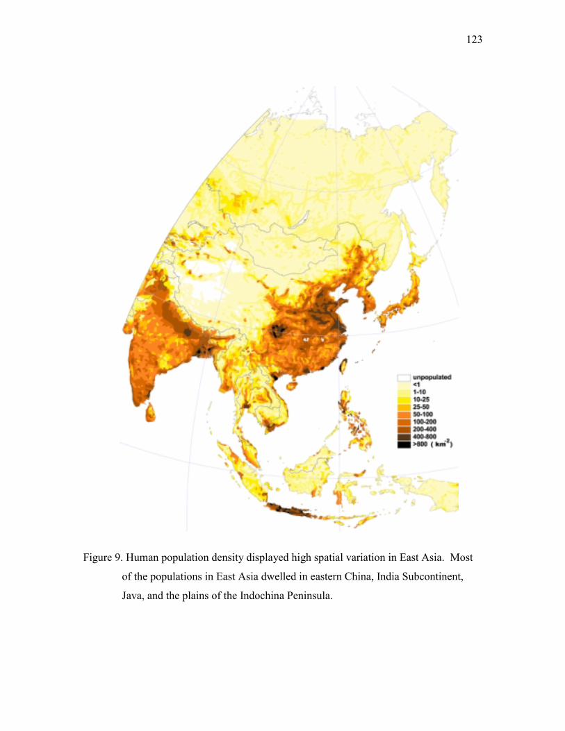
123

Figure 9. Human population density displayed high spatial variation in East Asia. Most

of the populations in East Asia dwelled in eastern China, India Subcontinent,

Java, and the plains of the Indochina Peninsula.

124

Appendix 1

(1) By taxa: having global maps of species distribution range

Baker, K. 1997. Warblers of Europe, Asia, and North Africa. Princeton Univ. Press.

Princeton, USA.

Burton, J. A. 1973. Owls of the world, their evolution, structure, and ecology. Dutton,

USA.

Byers, C., J. Curson, and U. Olsson. 1995. Sparrows and buntings. Houghton Mifflin.

Boston, USA.

Chantler, P. and G. Driessens. 1995. Swifts: a guide to the swifts and treeswifts of the

world. Pica, Mountfield, UK.

Cleere, N. 1998. Nightjars: a guide to the nightjars, nighthawks, and their relatives. Yale

University Press, New Haven, USA.

Clement, P. 1993. Finches & sparrows: an identification guide. Princeton University

Press. Princeton, USA.

Delacour, J. 1977. The pheasants of the world. Spur. Hindhead, UK.

Del Joyo, J., A. Elliott, and J. Sargatal (eds.). 1992. Handbook of the Birds of the World:

- Vol.1: Ostrich to Ducks. Lynx Edicion. Barcelona, Spain.

Del Joyo, J., A. Elliott, and J. Sargatal (eds.). 1994. Handbook of the Birds of the World:

- Vol.2: New World Vultures to Guineafowl. Lynx Edicion. Barcelona, Spain.

Del Joyo, J., A. Elliott, and J. Sargatal (eds.). 1996. Handbook of the Birds of the World:

- Vol.3: Barn Owls to Hummingbirds. Lynx Edicion. Barcelona, Spain.

125

Del Joyo, J., A. Elliott, and J. Sargatal (eds.). 1997. Handbook of the Birds of the World:

- Vol.4: Sandgrouse to Cuckoos. Lynx Edicion. Barcelona, Spain.

Del Joyo, J., A. Elliott, and J. Sargatal (eds.). 1999. Handbook of the Birds of the World:

- Vol.5: Barn Owls to Hummingbirds. Lynx Edicion. Barcelona, Spain.

Fry, C. H. and K. Fry. 1992. Kingfishers, bee-eaters and rollers: a handbook. Christopher

Helm. London, UK.

Goodwin, D. 1982. Estrildid finches of the world. British Museum. London, UK.

Godwin, D. 1983. Pigeons, and doves of the world. British Museum. London. UK.

Hancock, J. A. 1978. The herons of the world. Harper & Row. New York, USA.

Hancock, J. A., and J. A. Kushlan. 1984. The herons handbook. Croom Helm. London,

UK.

Hancock, J. A., J. A. Kushlan, and M. P. Kahl. 1992. Storks, ibises and spoonbills of the

world. Academic Press. London, UK.

Harrap, S. and D. Quinn. 1995. Chickadees, tits, nuthatches, and treecreepers. Princeton

University Press. Princeton, USA.

Johnsgard, P. A. 1981. The plovers, sandpipers, and snipes of the world. University of

Nebraska Press. Lincoln, USA.

Johnsgard, P. A. 1983. The grouse of the world. University of Nebraska Press. Lincoln,

USA.

Johnsgard, P. A. 1988. The quails, patridges and francolins of the world. Oxford

University Press. Oxford, UK.

Johnsgard, P. A. 1991. Bustards, hemipodes, and sandgrouse. Oxford University Press.

Oxford, UK.

126

Johnsgard, P. A. 1999. The pheasants of the world. Smithsonia Inst. Press, Washington

D.C., USA.

Juniper, T. and M. Parr. 1998. Parrots: a guide to parrots of the world. Yale University

Press, New Haven, USA.

Kear, J. 1994. Ducks of the world. Houghton Mifflin. Boston, USA.

Kemp, A. C. 1995. The hornbills : Bucerotiformes. Oxford University Press. Oxford, UK.

Lambert, F. R. and M. Woodcock. 1996. Pittas, broadbills and asities. Pica, Mountfield.

UK.

Lefranc, N. 1997. Shrikes : a guide to the shrikes of the world. Yale University Press.

New Haven, US.

Madge, S. and H. Burn. 1994. Crows and jays: a guide to the crows, jays, and magpies of

the world. Houghton Mifflin. Boston, USA.

Marchant, J. 1986. Shorebirds : an identification guide to the waders of the world. Croom

Helm, London, UK.

Restall, R. 1997. Munias and mannikins. Yale University Press. New Haven, USA.

Soothill, E. and R. Soothill. 1990. Wading birds of the world. Blandford Press. Dorset,

UK.

Todd, F. S. 1999. Natural history of the waterfowl. San Diego Natural History Museum.

San Diego, USA.

Turner, A. K. 1989. A handbook to the swallows and martins of the world. Christopher

Helm, London, UK.

Winkler, W., D. A. Chistie, and D. Nurney. 1995. Woodpeckers, a guide to the

woodpeckers of the world. Houghton Mifflin. Boston, USA.

127

(2) By regions: maps of distribution range of all species within the region or country

Brazil, M. A. 1991. The birds of Japan. Helm. London, UK.

Cheng, Tso-hsin. 1987. A synopsis of the avifauna of China. Science Press. Beijing,

China

Flint, V. F., R. L. Boehme, Y. V. Kostin, A. A. Kuznetsov. 1984. A field guide to birds of

USSR. Princeton University Press. Princeton, USA.

Grimmett, R., C. Inskipp, and T. Inskipp. 1999. A guide to the birds of India, Pakistan,

Nepal, Bangladesh, Bhutan, Sri Lanka, and the Maldives. Princeton, USA.

Inskipp, C. and T. Inskipp. 1991. A guide to the birds of Nepal. Helm. London, UK.

Kennedy, R. S., P. C. Gonzales, E. C. Dickinson, H. C. Miranda, and T. H. Fisher. 2000.

A guide to the birds of the Philippines. Oxford University Press. New York,

USA.

Lekagul, B. and P. D. Round. 1991. A guide to the birds of Thailand. Karn Bhaet.

Bangkok, Thailand.

MacKinnon, J. and K. Phillipps. 2000. A field Guide to the birds of China. Oxford

University Press. New York, USA.

Ranjit, D. R. 1997. A field guide to the birds of southwestern. Oxford University Press.

Oxford, UK.

Ripley, S. D. 1982. A synopsis of the birds of India and Pakistan : together with those of

Nepal, Bhutan, Bangladesh, and Sri Lanka. Bombay Natural History Society,

Bombay. India.

128

Wild Bird Society of Japan. 1982. A field guide to the birds of Japan. Kodansha. Tokyo,

Japan.

(3) textual description of distribution ranges

Ali, S. 1968. Handbook of the birds of India and Pakistan, together with those of Nepal,

Sikkim, Bhutan and Ceylon. Oxford University Press. Oxford, UK.

Ali, S. 1977. Field guide to the birds of the eastern Himalayas. Oxford University Press.

Oxford, UK.

Ali, S. 1996. The book of Indian Birds. Bombay Natural History Society. Bombay, India.

Bucknill, J. A. S. and F. N. Chasen. 1990. Birds of Singapore and South-East Asia. New

Holland. London, UK.

Holmes, D. 1989. The birds of Java and Bali. Oxford University Press. Oxford, UK.

Holmes, D. and K. Phillips. 1996. The birds of Sulawesi. Oxford University Press,

Oxford, UK.

Howards R.and A. Moore. 1991. A Complete Checklist of the Birds of the World. 2nd

Edition. Academic Press. San Diego, USA.

King, B. F. and E. C. Dickinson. 1975. Birds of South-East Asia. HarperCollins. London,

UK.

MacKinnon, J. 1990. Birds of Java and Bali. Gadjan Mada Univerdity Press. Yogyakarta,

Indonesia.

MacKinnon, J. and K. Phillips. 1993. A field guide to the birds of Borneo, Sumatra, Java,

and Bali, the Greater Sunda Islands. Oxford University Press, Oxford, UK

Mason, V. and F. Jarvis. 1989. Birds of Bali. Perilpus. Hong Kong, China.

129

Meyer de Schauensee, R. 1984. The birds of China. Smithsonian Press. Washington D.C.,

USA.

Rabor, D. S. 1977. Philippine birds and mammals. University of the Philippines Press.

Quezon City, Philippines.

Robson, C. 2000. A guide to the birds of Southeast Asia. Princeton University Press.

Princeton, USA.

Sibley, C. G. and B. L. Monroe. 1990. Distribution and Taxonomy of Birds of the World.

Yale University Press. New Heaven, USA.

van Marle, J. G. and K. H. Voous. 1988. The birds of Sumatra. British Ornithologists

Union. London, UK.

Yoon, M-B. 1995. Wildbirds of Korea. Kyo-Hak. Seoul, Korea.