Embed Size (px)
Citation preview
50
4c h a p t e r
Specific Factors and IncomeDistribution
A s we saw in Chapter 3, international trade can be mutually beneficial tothe nations engaged in it. Yet throughout history, governments haveprotected sectors of the economy from import competition. For example,
despite its commitment in principle to free trade, the United States limits importsof textiles, sugar, steel, and other commodities. If trade is such a good thing forthe economy, why is there opposition to its effects? To understand the politics oftrade, it is necessary to look at the effects of trade not just on a country as awhole, but on the distribution of income within that country.
The Ricardian model of international trade developed in Chapter 3 illustratesthe potential benefits from trade. In that model, trade leads to international spe-cialization, with each country shifting its labor force from industries in whichthat labor is relatively inefficient to industries in which it is relatively more effi-cient. Because labor is the only factor of production in that model, and it isassumed that labor can move freely from one industry to another, there is nopossibility that individuals will be hurt by trade. The Ricardian model thus sug-gests not only that all countries gain from trade, but also that every individual ismade better off as a result of international trade, because trade does not affectthe distribution of income. In the real world, however, trade has substantialeffects on the income distribution within each trading nation, so that in practicethe benefits of trade are often distributed very unevenly.
There are two main reasons why international trade has strong effects on thedistribution of income. First, resources cannot move immediately or without costfrom one industry to another—a short-run consequence of trade. Second, indus-tries differ in the factors of production they demand. A shift in the mix of goodsthat a country produces will ordinarily reduce the demand for some factors ofproduction, while raising the demand for others—a long-run consequence oftrade. For both of these reasons, international trade is not as unambiguously ben-eficial as it appeared to be in Chapter 3. While trade may benefit a nation as awhole, it often hurts significant groups within the country in the short run, andpotentially, but to a lesser extent, in the long run.
M04_KRUG6654_09_SE_C04.QXD 9/21/10 9:30 AM Page 50
CHAPTER 4 Specific Factors and Income Distribution 51
Consider the effects of Japan’s rice policy. Japan allows very little rice to beimported, even though the scarcity of land means that rice is much more expen-sive to produce in Japan than in other countries (including the United States).There is little question that Japan as a whole would have a higher standard ofliving if free imports of rice were allowed. Japanese rice farmers, however,would be hurt by free trade. While the farmers displaced by imports could prob-ably find jobs in manufacturing or services, they would find changing employ-ment costly and inconvenient: The special skills they developed for rice farmingwould be useless in those other jobs. Furthermore, the value of the land that thefarmers own would fall along with the price of rice. Not surprisingly, Japaneserice farmers are vehemently opposed to free trade in rice, and their organizedpolitical opposition has counted for more than the potential gains from trade forthe nation as a whole.
A realistic analysis of trade must go beyond the Ricardian model to models inwhich trade can affect income distribution. In this chapter, we focus on theshort-run consequences of trade on the income distribution when factors of pro-duction cannot move without cost between sectors. To keep our model simple,we assume that the sector-switching cost for some factors is high enough thatsuch a switch is impossible in the short run. Those factors are specific to a partic-ular sector.
LEARNING GOALS
After reading this chapter, you will be able to:
• Understand how a mobile factor will respond to price changes by movingacross sectors.
• Explain why trade will generate both winners and losers in the short run.• Understand the meaning of gains from trade when there are losers.• Discuss the reasons why trade is a politically contentious issue.• Explain the arguments in favor of free trade despite the existence of losers.
The Specific Factors ModelThe specific factors model was developed by Paul Samuelson and Ronald Jones.1 Likethe simple Ricardian model, it assumes an economy that produces two goods and that canallocate its labor supply between the two sectors. Unlike the Ricardian model, however,the specific factors model allows for the existence of factors of production besides labor.Whereas labor is a mobile factor that can move between sectors, these other factors areassumed to be specific. That is, they can be used only in the production of particulargoods.
1Paul Samuelson, “Ohlin Was Right,” Swedish Journal of Economics 73 (1971), pp. 365–384; and Ronald W.Jones, “A Three-Factor Model in Theory, Trade, and History,” in Jagdish Bhagwati et al., eds., Trade, Balance ofPayments, and Growth (Amsterdam: North-Holland, 1971), pp. 3–21.
M04_KRUG6654_09_SE_C04.QXD 9/21/10 9:30 AM Page 51
*See Bruce Fallick, “The Industrial Mobility of Displaced Workers,” Journal of Labor Economics 11 (April 1993), pp. 302–323.†See Gueorgui Kambourov and Iourii Manovskii, “Occupational Specificty of Huamn Capital,” International EconomicReview 50 (February 2009), pp. 63–115.
Worker mobility varies greatly with the charac-teristics of the worker (such as age) and the joboccupation (whether it requires general or job-specific skills). Nevertheless, one can measure anaverage rate of mobility by looking at the durationof unemployment following a worker’s displace-ment. After four years, a displaced worker in theUnited States has the same probability of be-ing employed as a similar worker who was notdisplaced.* This four-year time-span compares witha lifetime of 15 or 20 years for a typical specializedmachine, and 30 to 50 years for structures (a shop-ping mall, office building, or production plant).So labor is certainly a less specific factor than mostkinds of capital. However, even though most wor-kers can find new employment in other sectorswithin a four-year time-span, switching occupationsentails additional costs: A displaced worker who isre-employed in a different occupation suffers an18 percent permanent drop in wages (on average).This compares with a 6 percent drop if the workerdoes not switch occupations.† Thus, labor is trulyflexible only before a worker has invested in anyoccupation-specific skills.
52 PART ONE International Trade Theory
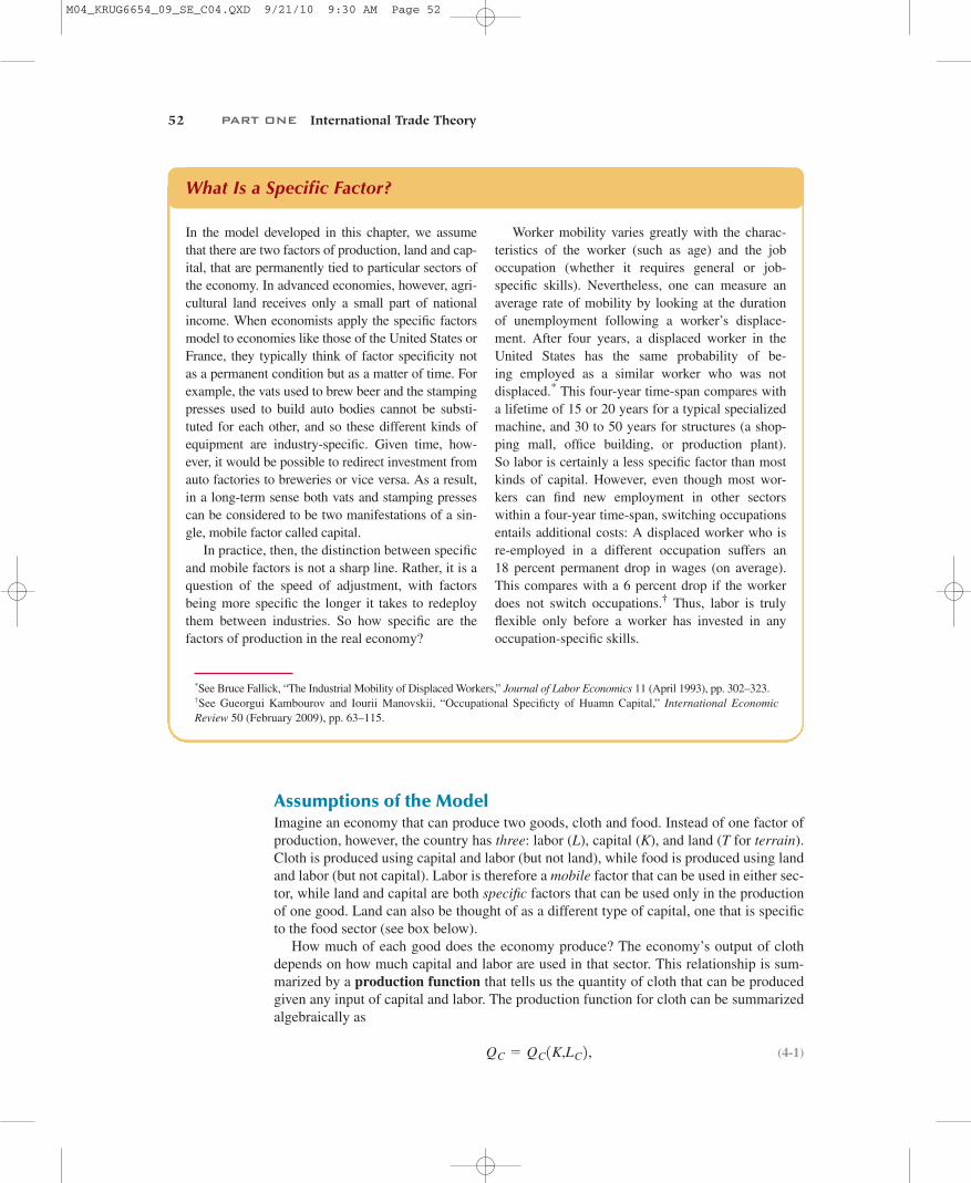
Assumptions of the ModelImagine an economy that can produce two goods, cloth and food. Instead of one factor ofproduction, however, the country has three: labor (L), capital (K), and land (T for terrain).Cloth is produced using capital and labor (but not land), while food is produced using landand labor (but not capital). Labor is therefore a mobile factor that can be used in either sec-tor, while land and capital are both specific factors that can be used only in the productionof one good. Land can also be thought of as a different type of capital, one that is specificto the food sector (see box below).
How much of each good does the economy produce? The economy’s output of clothdepends on how much capital and labor are used in that sector. This relationship is sum-marized by a production function that tells us the quantity of cloth that can be producedgiven any input of capital and labor. The production function for cloth can be summarizedalgebraically as
(4-1)QC = QC1K,LC2,
In the model developed in this chapter, we assumethat there are two factors of production, land and cap-ital, that are permanently tied to particular sectors ofthe economy. In advanced economies, however, agri-cultural land receives only a small part of nationalincome. When economists apply the specific factorsmodel to economies like those of the United States orFrance, they typically think of factor specificity notas a permanent condition but as a matter of time. Forexample, the vats used to brew beer and the stampingpresses used to build auto bodies cannot be substi-tuted for each other, and so these different kinds ofequipment are industry-specific. Given time, how-ever, it would be possible to redirect investment fromauto factories to breweries or vice versa. As a result,in a long-term sense both vats and stamping pressescan be considered to be two manifestations of a sin-gle, mobile factor called capital.
In practice, then, the distinction between specificand mobile factors is not a sharp line. Rather, it is aquestion of the speed of adjustment, with factorsbeing more specific the longer it takes to redeploythem between industries. So how specific are thefactors of production in the real economy?
What Is a Specific Factor?
M04_KRUG6654_09_SE_C04.QXD 9/21/10 9:30 AM Page 52
2Diminishing returns to a single factor does not imply diminishing returns to scale when all factors of productionare adjusted. Thus, diminishing returns to labor is entirely consistent with constant returns to scale in both laborand capital.
CHAPTER 4 Specific Factors and Income Distribution 53
where is the economy’s output of cloth, K is the economy’s capital stock, and is thelabor force employed in cloth. Similarly, for food we can write the production function
(4-2)
where is the economy’s output of food, T is the economy’s supply of land, and is the labor force devoted to food production. For the economy as a whole, the laboremployed must equal the total labor supply L:
(4-3)
Production PossibilitiesThe specific factors model assumes that each of the specific factors, capital and land, canbe used in only one sector, cloth and food, respectively. Only labor can be used in eithersector. Thus to analyze the economy’s production possibilities, we need only to ask howthe economy’s mix of output changes as labor is shifted from one sector to the other. Thiscan be done graphically, first by representing the production functions (4-1) and (4-2), andthen by putting them together to derive the production possibility frontier.
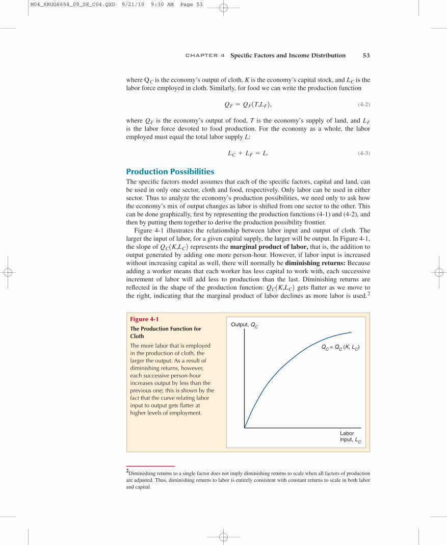
Figure 4-1 illustrates the relationship between labor input and output of cloth. Thelarger the input of labor, for a given capital supply, the larger will be output. In Figure 4-1,the slope of represents the marginal product of labor, that is, the addition tooutput generated by adding one more person-hour. However, if labor input is increasedwithout increasing capital as well, there will normally be diminishing returns: Becauseadding a worker means that each worker has less capital to work with, each successiveincrement of labor will add less to production than the last. Diminishing returns arereflected in the shape of the production function: gets flatter as we move tothe right, indicating that the marginal product of labor declines as more labor is used.2
QC1K,LC2
QC1K,LC2
LC + LF = L.
LFQF
QF = QF1T,LF2,
LCQC
Output, QC
Labor input, LC
QC = QC (K, LC)
Figure 4-1
The Production Function forCloth
The more labor that is employedin the production of cloth, thelarger the output. As a result ofdiminishing returns, however,each successive person-hourincreases output by less than theprevious one; this is shown by thefact that the curve relating laborinput to output gets flatter athigher levels of employment.
M04_KRUG6654_09_SE_C04.QXD 9/21/10 9:30 AM Page 53
54 PART ONE International Trade Theory
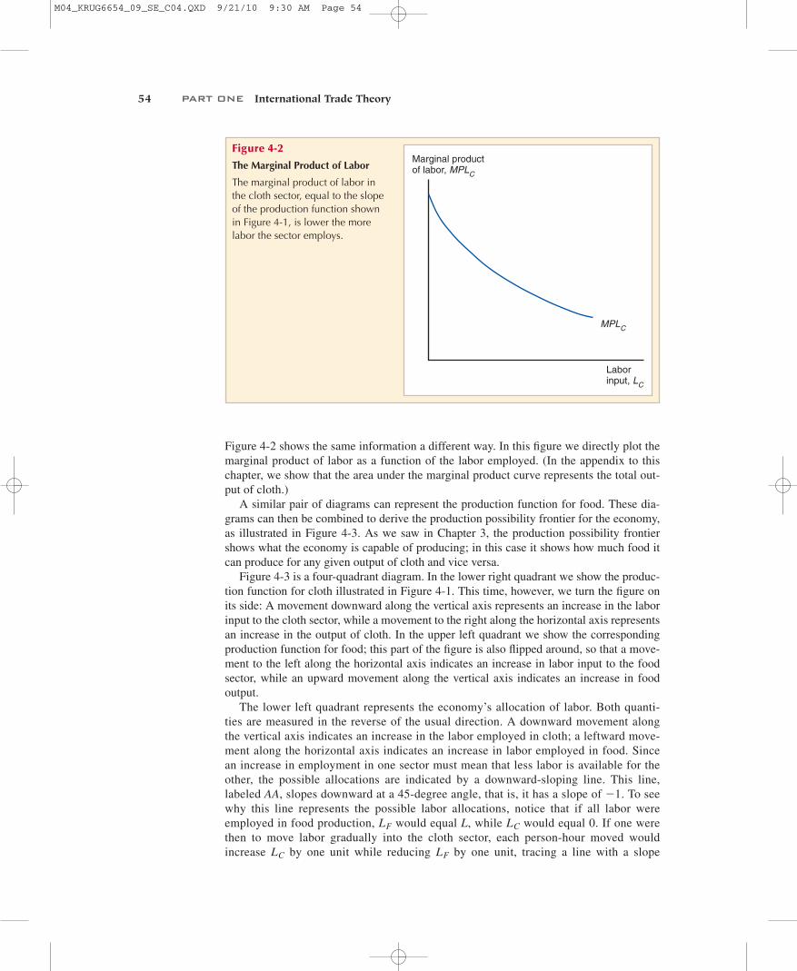
Figure 4-2 shows the same information a different way. In this figure we directly plot themarginal product of labor as a function of the labor employed. (In the appendix to thischapter, we show that the area under the marginal product curve represents the total out-put of cloth.)
A similar pair of diagrams can represent the production function for food. These dia-grams can then be combined to derive the production possibility frontier for the economy,as illustrated in Figure 4-3. As we saw in Chapter 3, the production possibility frontiershows what the economy is capable of producing; in this case it shows how much food itcan produce for any given output of cloth and vice versa.
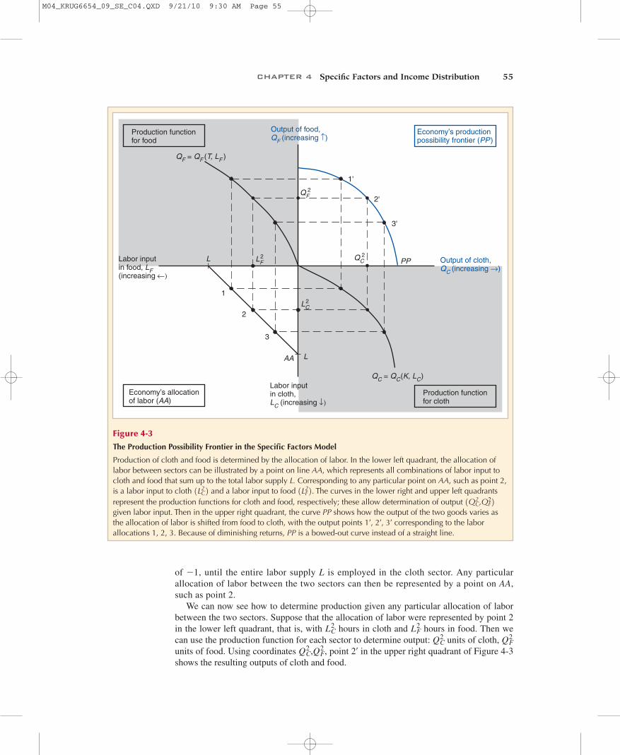
Figure 4-3 is a four-quadrant diagram. In the lower right quadrant we show the produc-tion function for cloth illustrated in Figure 4-1. This time, however, we turn the figure onits side: A movement downward along the vertical axis represents an increase in the laborinput to the cloth sector, while a movement to the right along the horizontal axis representsan increase in the output of cloth. In the upper left quadrant we show the correspondingproduction function for food; this part of the figure is also flipped around, so that a move-ment to the left along the horizontal axis indicates an increase in labor input to the foodsector, while an upward movement along the vertical axis indicates an increase in foodoutput.
The lower left quadrant represents the economy’s allocation of labor. Both quanti-ties are measured in the reverse of the usual direction. A downward movement alongthe vertical axis indicates an increase in the labor employed in cloth; a leftward move-ment along the horizontal axis indicates an increase in labor employed in food. Sincean increase in employment in one sector must mean that less labor is available for theother, the possible allocations are indicated by a downward-sloping line. This line,labeled AA, slopes downward at a 45-degree angle, that is, it has a slope of . To seewhy this line represents the possible labor allocations, notice that if all labor wereemployed in food production, would equal L, while would equal 0. If one werethen to move labor gradually into the cloth sector, each person-hour moved wouldincrease by one unit while reducing by one unit, tracing a line with a slope LFLC
LCLF
-1
Marginal productof labor, MPLC
MPLC
Labor input, LC
Figure 4-2
The Marginal Product of Labor
The marginal product of labor inthe cloth sector, equal to the slopeof the production function shownin Figure 4-1, is lower the morelabor the sector employs.
M04_KRUG6654_09_SE_C04.QXD 9/21/10 9:30 AM Page 54
CHAPTER 4 Specific Factors and Income Distribution 55
Labor inputin food, LF (increasing ←)
Labor inputin cloth,LC (increasing ↓)
1'
2
3
1
2'
3'
L
AA L
PP
QF = QF (T, LF )
QC = QC(K, LC)
Economy’s allocationof labor (AA)
Production functionfor food
Production functionfor cloth
Output of food,QF (increasing ↑)
Output of cloth,QC (increasing →)
Economy’s productionpossibility frontier (PP)
LF2
LC2
QF2
QC2
Figure 4-3
The Production Possibility Frontier in the Specific Factors Model
Production of cloth and food is determined by the allocation of labor. In the lower left quadrant, the allocation oflabor between sectors can be illustrated by a point on line AA, which represents all combinations of labor input tocloth and food that sum up to the total labor supply L. Corresponding to any particular point on AA, such as point 2,is a labor input to cloth and a labor input to food . The curves in the lower right and upper left quadrantsrepresent the production functions for cloth and food, respectively; these allow determination of output given labor input. Then in the upper right quadrant, the curve PP shows how the output of the two goods varies asthe allocation of labor is shifted from food to cloth, with the output points 1¿, 2¿, 3¿ corresponding to the laborallocations 1, 2, 3. Because of diminishing returns, PP is a bowed-out curve instead of a straight line.
1QC2,QF
22
1LF221LC
22
of , until the entire labor supply L is employed in the cloth sector. Any particularallocation of labor between the two sectors can then be represented by a point on AA,such as point 2.
We can now see how to determine production given any particular allocation of laborbetween the two sectors. Suppose that the allocation of labor were represented by point 2in the lower left quadrant, that is, with hours in cloth and hours in food. Then wecan use the production function for each sector to determine output: units of cloth, units of food. Using coordinates , point 2¿ in the upper right quadrant of Figure 4-3shows the resulting outputs of cloth and food.
QC2 ,QF
2QF
2QC2
LF2LC
2
-1
M04_KRUG6654_09_SE_C04.QXD 9/21/10 9:30 AM Page 55
56 PART ONE International Trade Theory
To trace the whole production possibility frontier, we simply imagine repeating thisexercise for many alternative allocations of labor. We might start with most of the laborallocated to food production, as at point 1 in the lower left quadrant, then graduallyincrease the amount of labor used in cloth until very few workers are employed in food, asat point 3; the corresponding points in the upper right quadrant will trace out the curverunning from 1¿ to 3¿. Thus PP in the upper right quadrant shows the economy’s produc-tion possibilities for given supplies of land, labor, and capital.
In the Ricardian model, where labor is the only factor of production, the productionpossibility frontier is a straight line because the opportunity cost of cloth in terms of foodis constant. In the specific factors model, however, the addition of other factors of produc-tion changes the shape of the production possibility frontier PP to a curve. The curvatureof PP reflects diminishing returns to labor in each sector; these diminishing returns are thecrucial difference between the specific factors and the Ricardian models.
Notice that when tracing PP we shift labor from the food to the cloth sector. If weshift one person-hour of labor from food to cloth, however, this extra input willincrease output in that sector by the marginal product of labor in cloth, . Toincrease cloth output by one unit, then, we must increase labor input by hours.Meanwhile, each unit of labor input shifted out of food production will lower output inthat sector by the marginal product of labor in food, . To increase output of clothby one unit, then, the economy must reduce output of food by units. Theslope of PP, which measures the opportunity cost of cloth in terms of food—that is, thenumber of units of food output that must be sacrificed to increase cloth output byone unit—is therefore
We can now see why PP has the bowed shape it does. As we move from l¿ to 3¿, risesand falls. We saw in Figure 4-2, however, that as rises, the marginal product of laborin cloth falls; correspondingly, as falls, the marginal product of labor in food rises. Asmore and more labor is moved to the cloth sector, each additional unit of labor becomesless valuable in the cloth sector and more valuable in the food sector: The opportunity cost(foregone food production) of each additional cloth unit rises, and PP thus gets steeper aswe move down it to the right.
We have now shown how output is determined, given the allocation of labor. The nextstep is to ask how a market economy determines what the allocation of labor should be.
Prices, Wages, and Labor AllocationHow much labor will be employed in each sector? To answer this we need to look at sup-ply and demand in the labor market. The demand for labor in each sector depends on theprice of output and the wage rate. In turn, the wage rate depends on the combined demandfor labor by food and cloth producers. Given the prices of cloth and food together with thewage rate, we can determine each sector’s employment and output.
First, let us focus on the demand for labor. In each sector, profit-maximizing employerswill demand labor up to the point where the value produced by an additional person-hourequals the cost of employing that hour. In the cloth sector, for example, the value of anadditional person-hour is the marginal product of labor in cloth multiplied by the price ofone unit of cloth: If w is the wage rate of labor, employers will therefore hireworkers up to the point where
(4-4)MPLC * PC = w.
MPLC * PC.
LF
LCLF
LC
Slope of production possibilities curve = -MPLF /MPLC.
MPLF /MPLC
MPLF
1/MPLC
MPLC
M04_KRUG6654_09_SE_C04.QXD 9/21/10 9:30 AM Page 56
CHAPTER 4 Specific Factors and Income Distribution 57
But the marginal product of labor in cloth, already illustrated in Figure 4-2, slopesdownward because of diminishing returns. So for any given price of cloth , the valueof that marginal product, will also slope down. We can therefore think ofequation (4-4) as defining the demand curve for labor in the cloth sector: If the wagerate falls, other things equal, employers in the cloth sector will want to hire moreworkers.
Similarly, the value of an additional person-hour in food is . The demandcurve for labor in the food sector may therefore be written
(4-5)
The wage rate w must be the same in both sectors, because of the assumption that laboris freely mobile between sectors. That is, because labor is a mobile factor, it will movefrom the low-wage sector to the high-wage sector until wages are equalized. The wagerate, in turn, is determined by the requirement that total labor demand (total employ-ment) equals total labor supply. This equilibrium condition for labor is represented inequation (4-3).
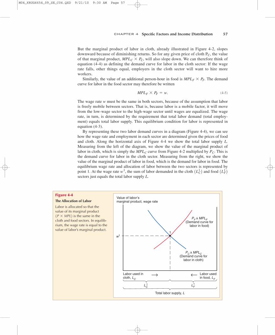
By representing these two labor demand curves in a diagram (Figure 4-4), we can seehow the wage rate and employment in each sector are determined given the prices of foodand cloth. Along the horizontal axis of Figure 4-4 we show the total labor supply L.Measuring from the left of the diagram, we show the value of the marginal product oflabor in cloth, which is simply the curve from Figure 4-2 multiplied by . This isthe demand curve for labor in the cloth sector. Measuring from the right, we show thevalue of the marginal product of labor in food, which is the demand for labor in food. Theequilibrium wage rate and allocation of labor between the two sectors is represented bypoint 1. At the wage rate , the sum of labor demanded in the cloth and food sectors just equals the total labor supply L.
1LF121LC
12w1
PCMPLC
MPLF * PF = w.
MPLF * PF
MPLC * PC,PC
Value of labor’smarginal product, wage rate
w11
PF x MPLF(Demand curve for
labor in food)
PC x MPLC(Demand curve for
labor in cloth)
Labor used incloth, LC
Labor usedin food, LF
Total labor supply, L
LC1 LF
1
Figure 4-4
The Allocation of Labor
Labor is allocated so that thevalue of its marginal product
is the same in thecloth and food sectors. In equilib-rium, the wage rate is equal to thevalue of labor’s marginal product.
1P * MPL2
M04_KRUG6654_09_SE_C04.QXD 9/21/10 9:30 AM Page 57
58 PART ONE International Trade Theory
Output of food, QF
Output of cloth,QC
PP
1
slope = –(PC/PF )1
QC1
QF1
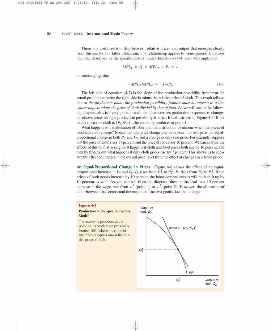
Figure 4-5
Production in the Specific FactorsModel
The economy produces at thepoint on its production possibilityfrontier where the slope ofthat frontier equals minus the rela-tive price of cloth.
(PP)
There is a useful relationship between relative prices and output that emerges clearlyfrom this analysis of labor allocation; this relationship applies to more general situationsthan that described by the specific factors model. Equations (4-4) and (4-5) imply that
or, rearranging, that
(4-6)
The left side of equation (4-7) is the slope of the production possibility frontier at theactual production point; the right side is minus the relative price of cloth. This result tells usthat at the production point, the production possibility frontier must be tangent to a linewhose slope is minus the price of cloth divided by that of food. As we will see in the follow-ing chapters, this is a very general result that characterizes production responses to changesin relative prices along a production possibility frontier. It is illustrated in Figure 4-5: If therelative price of cloth is , the economy produces at point 1.
What happens to the allocation of labor and the distribution of income when the prices offood and cloth change? Notice that any price change can be broken into two parts: an equal-proportional change in both and , and a change in only one price. For example, supposethat the price of cloth rises 17 percent and the price of food rises 10 percent. We can analyze theeffects of this by first asking what happens if cloth and food prices both rise by 10 percent, andthen by finding out what happens if only cloth prices rise by 7 percent. This allows us to sepa-rate the effect of changes in the overall price level from the effect of changes in relative prices.
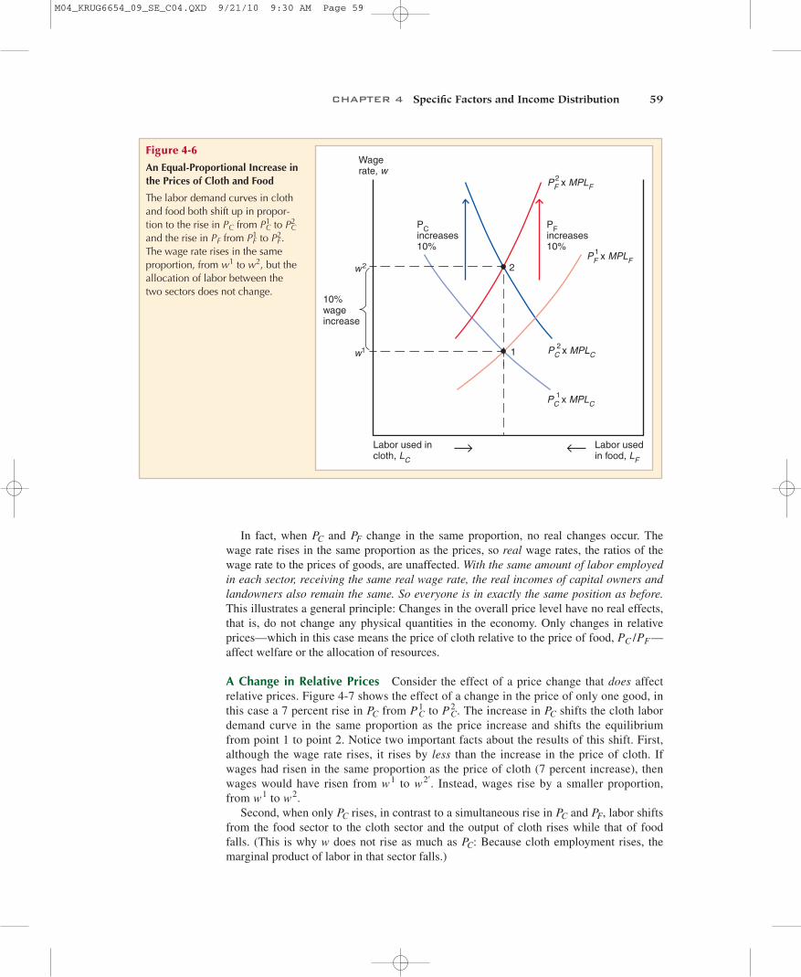
An Equal-Proportional Change in Prices Figure 4-6 shows the effect of an equal-proportional increase in and . rises from to ; rises from to . If theprices of both goods increase by 10 percent, the labor demand curves will both shift up by10 percent as well. As you can see from the diagram, these shifts lead to a 10 percentincrease in the wage rate from (point 1) to (point 2). However, the allocation oflabor between the sectors and the outputs of the two goods does not change.
w2w1
PF2PF
1PFPC2PC
1PCPFPC
PFPC
1PC /PF21
-MPLF /MPLC = -PC /PF.
MPLC * PC = MPLF * PF = w
M04_KRUG6654_09_SE_C04.QXD 9/21/10 9:30 AM Page 58
CHAPTER 4 Specific Factors and Income Distribution 59
In fact, when and change in the same proportion, no real changes occur. Thewage rate rises in the same proportion as the prices, so real wage rates, the ratios of thewage rate to the prices of goods, are unaffected. With the same amount of labor employedin each sector, receiving the same real wage rate, the real incomes of capital owners andlandowners also remain the same. So everyone is in exactly the same position as before.This illustrates a general principle: Changes in the overall price level have no real effects,that is, do not change any physical quantities in the economy. Only changes in relativeprices—which in this case means the price of cloth relative to the price of food, —affect welfare or the allocation of resources.
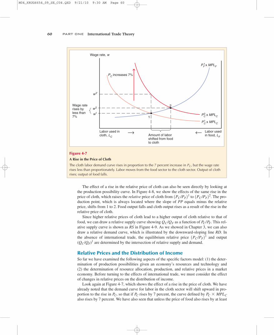
A Change in Relative Prices Consider the effect of a price change that does affectrelative prices. Figure 4-7 shows the effect of a change in the price of only one good, inthis case a 7 percent rise in from to . The increase in shifts the cloth labordemand curve in the same proportion as the price increase and shifts the equilibriumfrom point 1 to point 2. Notice two important facts about the results of this shift. First,although the wage rate rises, it rises by less than the increase in the price of cloth. Ifwages had risen in the same proportion as the price of cloth (7 percent increase), thenwages would have risen from to . Instead, wages rise by a smaller proportion,from to .
Second, when only rises, in contrast to a simultaneous rise in and , labor shiftsfrom the food sector to the cloth sector and the output of cloth rises while that of foodfalls. (This is why w does not rise as much as : Because cloth employment rises, themarginal product of labor in that sector falls.)
PC
PFPCPC
w2w1w2¿w1
PCPC2PC
1PC
PC /PF
PFPC
w1 1
Labor used incloth, LC
Labor usedin food, LF
w2 2
Wagerate, w
PFincreases10%
PCincreases10%
10% wage increase
PF x MPLF1
PF x MPLF2
PC x MPLC2
PC x MPLC1
Figure 4-6
An Equal-Proportional Increase inthe Prices of Cloth and Food
The labor demand curves in clothand food both shift up in propor-tion to the rise in from to and the rise in from to .The wage rate rises in the sameproportion, from to , but theallocation of labor between thetwo sectors does not change.
w2w1
PF2PF
1PF
PC2PC
1PC
M04_KRUG6654_09_SE_C04.QXD 9/21/10 9:30 AM Page 59
60 PART ONE International Trade Theory
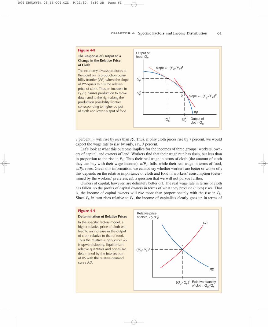
The effect of a rise in the relative price of cloth can also be seen directly by looking atthe production possibility curve. In Figure 4-8, we show the effects of the same rise in theprice of cloth, which raises the relative price of cloth from to . The pro-duction point, which is always located where the slope of PP equals minus the relativeprice, shifts from 1 to 2. Food output falls and cloth output rises as a result of the rise in therelative price of cloth.
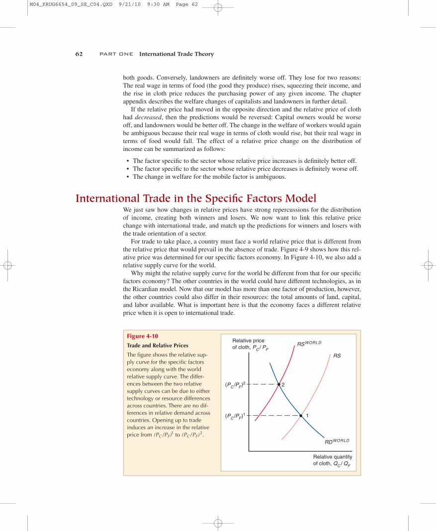
Since higher relative prices of cloth lead to a higher output of cloth relative to that offood, we can draw a relative supply curve showing as a function of . This rel-ative supply curve is shown as RS in Figure 4-9. As we showed in Chapter 3, we can alsodraw a relative demand curve, which is illustrated by the downward-sloping line RD. Inthe absence of international trade, the equilibrium relative price and output
are determined by the intersection of relative supply and demand.
Relative Prices and the Distribution of IncomeSo far we have examined the following aspects of the specific factors model: (1) the deter-mination of production possibilities given an economy’s resources and technology and (2) the determination of resource allocation, production, and relative prices in a marketeconomy. Before turning to the effects of international trade, we must consider the effectof changes in relative prices on the distribution of income.
Look again at Figure 4-7, which shows the effect of a rise in the price of cloth. We havealready noted that the demand curve for labor in the cloth sector will shift upward in pro-portion to the rise in , so that if rises by 7 percent, the curve defined by also rises by 7 percent. We have also seen that unless the price of food also rises by at least
PC * MPLCPCPC
(QC /QF)11PC /PF2
1
PC /PFQC /QF
1PC /PF221PC /PF2
1
Wage rate, w
w1
1
PF x MPLF
Labor used incloth, LC
Labor usedin food, LF
Amount of labor shifted from food to cloth
w2
w2�
Wage rate rises by less than 7%
PC increases 7%
2
1
PC x MPLC2
PC x MPLC1
Figure 4-7
A Rise in the Price of Cloth
The cloth labor demand curve rises in proportion to the 7 percent increase in , but the wage raterises less than proportionately. Labor moves from the food sector to the cloth sector. Output of clothrises; output of food falls.
PC
M04_KRUG6654_09_SE_C04.QXD 9/21/10 9:30 AM Page 60
CHAPTER 4 Specific Factors and Income Distribution 61
7 percent, w will rise by less than . Thus, if only cloth prices rise by 7 percent, we wouldexpect the wage rate to rise by only, say, 3 percent.
Let’s look at what this outcome implies for the incomes of three groups: workers, own-ers of capital, and owners of land. Workers find that their wage rate has risen, but less thanin proportion to the rise in . Thus their real wage in terms of cloth (the amount of cloththey can buy with their wage income), , falls, while their real wage in terms of food,
, rises. Given this information, we cannot say whether workers are better or worse off;this depends on the relative importance of cloth and food in workers’ consumption (deter-mined by the workers’ preferences), a question that we will not pursue further.
Owners of capital, however, are definitely better off. The real wage rate in terms of clothhas fallen, so the profits of capital owners in terms of what they produce (cloth) rises. Thatis, the income of capital owners will rise more than proportionately with the rise in .Since in turn rises relative to , the income of capitalists clearly goes up in terms ofPFPC
PC
w/PF
w/PC
PC
PC
QC2
Output of food, QF
Output of cloth, QC
PP
1
slope = –(PC/ PF )1
2
QC1
QF1
QF2
slope = –(PC / PF )2
Figure 4-8
The Response of Output to aChange in the Relative Price of Cloth
The economy always produces atthe point on its production possi-bility frontier where the slopeof PP equals minus the relativeprice of cloth. Thus an increase in
causes production to movedown and to the right along theproduction possibility frontiercorresponding to higher output of cloth and lower output of food.
PC/PF
1PP2
Relative priceof cloth, PC /PF
1(PC/ PF )1
Relative quantityof cloth, QC /QF
(QC / QF )1
RS
RD
Figure 4-9
Determination of Relative Prices
In the specific factors model, ahigher relative price of cloth willlead to an increase in the outputof cloth relative to that of food.Thus the relative supply curve RSis upward sloping. Equilibriumrelative quantities and prices aredetermined by the intersection of RS with the relative demandcurve RD.
M04_KRUG6654_09_SE_C04.QXD 9/21/10 9:30 AM Page 61
62 PART ONE International Trade Theory
both goods. Conversely, landowners are definitely worse off. They lose for two reasons:The real wage in terms of food (the good they produce) rises, squeezing their income, andthe rise in cloth price reduces the purchasing power of any given income. The chapterappendix describes the welfare changes of capitalists and landowners in further detail.
If the relative price had moved in the opposite direction and the relative price of clothhad decreased, then the predictions would be reversed: Capital owners would be worseoff, and landowners would be better off. The change in the welfare of workers would againbe ambiguous because their real wage in terms of cloth would rise, but their real wage interms of food would fall. The effect of a relative price change on the distribution ofincome can be summarized as follows:
• The factor specific to the sector whose relative price increases is definitely better off.• The factor specific to the sector whose relative price decreases is definitely worse off.• The change in welfare for the mobile factor is ambiguous.
International Trade in the Specific Factors ModelWe just saw how changes in relative prices have strong repercussions for the distributionof income, creating both winners and losers. We now want to link this relative pricechange with international trade, and match up the predictions for winners and losers withthe trade orientation of a sector.
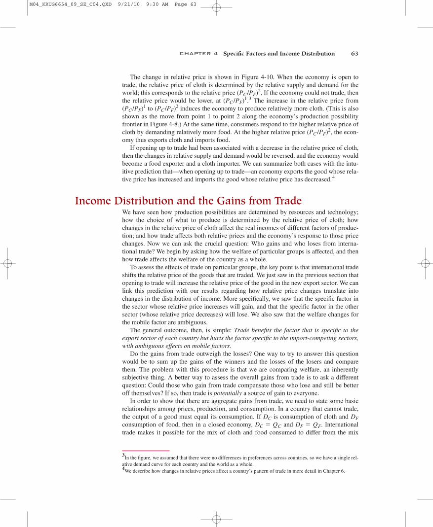
For trade to take place, a country must face a world relative price that is different fromthe relative price that would prevail in the absence of trade. Figure 4-9 shows how this rel-ative price was determined for our specific factors economy. In Figure 4-10, we also add arelative supply curve for the world.
Why might the relative supply curve for the world be different from that for our specificfactors economy? The other countries in the world could have different technologies, as inthe Ricardian model. Now that our model has more than one factor of production, however,the other countries could also differ in their resources: the total amounts of land, capital,and labor available. What is important here is that the economy faces a different relativeprice when it is open to international trade.
Relative priceof cloth, PC / PF
Relative quantityof cloth, QC / QF
(PC /PF)1
(PC /PF)2 2
1
RS
RSWORLD
RDWORLD
Figure 4-10
Trade and Relative Prices
The figure shows the relative sup-ply curve for the specific factorseconomy along with the worldrelative supply curve. The differ-ences between the two relativesupply curves can be due to eithertechnology or resource differencesacross countries. There are no dif-ferences in relative demand acrosscountries. Opening up to tradeinduces an increase in the relativeprice from to .(PC/PF)
2(PC/PF)1
M04_KRUG6654_09_SE_C04.QXD 9/21/10 9:30 AM Page 62
CHAPTER 4 Specific Factors and Income Distribution 63
The change in relative price is shown in Figure 4-10. When the economy is open totrade, the relative price of cloth is determined by the relative supply and demand for theworld; this corresponds to the relative price . If the economy could not trade, thenthe relative price would be lower, at .3 The increase in the relative price from
to induces the economy to produce relatively more cloth. (This is alsoshown as the move from point 1 to point 2 along the economy’s production possibilityfrontier in Figure 4-8.) At the same time, consumers respond to the higher relative price ofcloth by demanding relatively more food. At the higher relative price , the econ-omy thus exports cloth and imports food.
If opening up to trade had been associated with a decrease in the relative price of cloth,then the changes in relative supply and demand would be reversed, and the economy wouldbecome a food exporter and a cloth importer. We can summarize both cases with the intu-itive prediction that—when opening up to trade—an economy exports the good whose rela-tive price has increased and imports the good whose relative price has decreased.4
Income Distribution and the Gains from TradeWe have seen how production possibilities are determined by resources and technology;how the choice of what to produce is determined by the relative price of cloth; howchanges in the relative price of cloth affect the real incomes of different factors of produc-tion; and how trade affects both relative prices and the economy’s response to those pricechanges. Now we can ask the crucial question: Who gains and who loses from interna-tional trade? We begin by asking how the welfare of particular groups is affected, and thenhow trade affects the welfare of the country as a whole.
To assess the effects of trade on particular groups, the key point is that international tradeshifts the relative price of the goods that are traded. We just saw in the previous section thatopening to trade will increase the relative price of the good in the new export sector. We canlink this prediction with our results regarding how relative price changes translate intochanges in the distribution of income. More specifically, we saw that the specific factor inthe sector whose relative price increases will gain, and that the specific factor in the othersector (whose relative price decreases) will lose. We also saw that the welfare changes forthe mobile factor are ambiguous.
The general outcome, then, is simple: Trade benefits the factor that is specific to theexport sector of each country but hurts the factor specific to the import-competing sectors,with ambiguous effects on mobile factors.
Do the gains from trade outweigh the losses? One way to try to answer this questionwould be to sum up the gains of the winners and the losses of the losers and comparethem. The problem with this procedure is that we are comparing welfare, an inherentlysubjective thing. A better way to assess the overall gains from trade is to ask a differentquestion: Could those who gain from trade compensate those who lose and still be betteroff themselves? If so, then trade is potentially a source of gain to everyone.
In order to show that there are aggregate gains from trade, we need to state some basicrelationships among prices, production, and consumption. In a country that cannot trade,the output of a good must equal its consumption. If is consumption of cloth and consumption of food, then in a closed economy, and . Internationaltrade makes it possible for the mix of cloth and food consumed to differ from the mix
DF = QFDC = QC
DFDC
(PC /PF)2
(PC /PF)2(PC /PF)1(PC /PF)1
(PC /PF)2
3In the figure, we assumed that there were no differences in preferences across countries, so we have a single rel-ative demand curve for each country and the world as a whole.4We describe how changes in relative prices affect a country’s pattern of trade in more detail in Chapter 6.
M04_KRUG6654_09_SE_C04.QXD 9/21/10 9:30 AM Page 63
64 PART ONE International Trade Theory
produced. While the amounts of each good that a country consumes and produces maydiffer, however, a country cannot spend more than it earns: The value of consumptionmust be equal to the value of production. That is,
(4-7)
Equation (4-8) can be rearranged to yield the following:
(4-8)
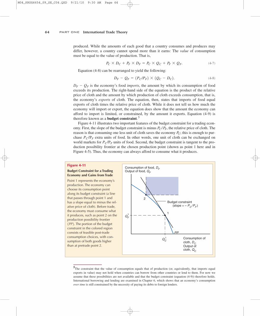
is the economy’s food imports, the amount by which its consumption of foodexceeds its production. The right-hand side of the equation is the product of the relativeprice of cloth and the amount by which production of cloth exceeds consumption, that is,the economy’s exports of cloth. The equation, then, states that imports of food equalexports of cloth times the relative price of cloth. While it does not tell us how much theeconomy will import or export, the equation does show that the amount the economy canafford to import is limited, or constrained, by the amount it exports. Equation (4-9) istherefore known as a budget constraint.5
Figure 4-11 illustrates two important features of the budget constraint for a trading econ-omy. First, the slope of the budget constraint is minus , the relative price of cloth. Thereason is that consuming one less unit of cloth saves the economy ; this is enough to pur-chase extra units of food. In other words, one unit of cloth can be exchanged onworld markets for units of food. Second, the budget constraint is tangent to the pro-duction possibility frontier at the chosen production point (shown as point 1 here and inFigure 4-5). Thus, the economy can always afford to consume what it produces.
PC/PF
PC /PF
PC
PC /PF
DF - QF
DF - QF = 1PC /PF2 * 1QC - DC2.
PC * DC + PF * DF = PC * QC + PF * QF.
5The constraint that the value of consumption equals that of production (or, equivalently, that imports equalexports in value) may not hold when countries can borrow from other countries or lend to them. For now weassume that these possibilities are not available and that the budget constraint (equation (4-9)) therefore holds.International borrowing and lending are examined in Chapter 6, which shows that an economy’s consumptionover time is still constrained by the necessity of paying its debts to foreign lenders.
Consumption of food, DFOutput of food, QF
Consumption ofcloth, DCOutput ofcloth, QC
PP
1
Budget constraint (slope = – PC/PF )
2
QC1
QF1
Figure 4-11
Budget Constraint for a TradingEconomy and Gains from Trade
Point 1 represents the economy’sproduction. The economy canchoose its consumption pointalong its budget constraint (a linethat passes through point 1 andhas a slope equal to minus the rel-ative price of cloth). Before trade,the economy must consume whatit produces, such as point 2 on theproduction possibility frontier
. The portion of the budgetconstraint in the colored regionconsists of feasible post-tradeconsumption choices, with con-sumption of both goods higherthan at pretrade point 2.
1PP2
M04_KRUG6654_09_SE_C04.QXD 9/21/10 9:30 AM Page 64
CHAPTER 4 Specific Factors and Income Distribution 65
To illustrate that trade is a source of potential gain for everyone, we proceed in threesteps:
1. First, we notice that in the absence of trade, the economy would have to produce whatit consumed, and vice versa. Thus the consumption of the economy in the absence oftrade would have to be a point on the production possibility frontier. In Figure 4-11, atypical pretrade consumption point is shown as point 2.
2. Next, we notice that it is possible for a trading economy to consume more of both goodsthan it would have in the absence of trade. The budget constraint in Figure 4-11 repre-sents all the possible combinations of food and cloth that the country could consumegiven the world relative price of cloth. Part of that budget constraint—the part in the col-ored region—represents situations in which the economy consumes more of both clothand food than it could in the absence of trade. Notice that this result does not depend onthe assumption that pretrade production and consumption is at point 2; unless pretradeproduction is at point 1, so that trade has no effect on production at all, there is always apart of the budget constraint that allows the consumption of more of both goods.
3. Finally, observe that if the economy as a whole consumes more of both goods, then itis possible in principle to give each individual more of both goods. This would makeeveryone better off. This shows, then, that it is possible to ensure that everyone is bet-ter off as a result of trade. Of course, everyone might be even better off if they had lessof one good and more of the other, but this only reinforces the conclusion that every-one has the potential to gain from trade.
The fundamental reason why trade potentially benefits a country is that it expands theeconomy’s choices. This expansion of choice means that it is always possible to redistrib-ute income in such a way that everyone gains from trade.6
That everyone could gain from trade unfortunately does not mean that everyone actu-ally does. In the real world, the presence of losers as well as winners from trade is one ofthe most important reasons why trade is not free.
The Political Economy of Trade: A Preliminary ViewTrade often produces losers as well as winners. This insight is crucial to understanding theconsiderations that actually determine trade policy in the modern world economy. Our spe-cific factors model informs us that those who stand to lose most from trade are the immobilefactors in the import-competing sector. In the real world, this includes not only the owners ofcapital, but also a portion of the labor force in those importing-competing sectors. Some ofthose workers have a hard time transitioning from the import-competing sectors (where tradeinduces reductions in employment) to export sectors (where trade induces increases inemployment). Some suffer unemployment spells as a result. In the United States, workers inthe import-competing sectors earn wages that are substantially below the average wage. (Forexample, the average wage in the apparel sector in 2009 was 36 percent below the averagewage across all manufacturing sectors.) One result of this disparity in wages is widespreadsympathy for the plight of those workers and, consequently, for restrictions on apparelimports. The gains that more affluent consumers would realize if more imports were allowedand the associated increases in employment in the export sectors (which hire, on average,relatively higher-skilled workers) do not matter as much.
6The argument that trade is beneficial because it enlarges an economy’s choices is much more general than thisspecific example. For a thorough discussion, see Paul Samuelson, “The Gains from International Trade OnceAgain,” Economic Journal 72 (1962), pp. 820–829.
M04_KRUG6654_09_SE_C04.QXD 9/21/10 9:30 AM Page 65
66 PART ONE International Trade Theory
Does this mean that trade should be allowed only if it doesn’t hurt lower-income people?Few international economists would agree. In spite of the real importance of income distri-bution, most economists remain strongly in favor of more or less free trade. There are threemain reasons why economists do not generally stress the income distribution effects of trade:
1. Income distribution effects are not specific to international trade. Every change in a na-tion’s economy, including technological progress, shifting consumer preferences,exhaustion of old resources and discovery of new ones, and so on, affects income distri-bution. Why should an apparel worker, who suffers an unemployment spell due to in-creased import competition, be treated differently from an unemployed printing machineoperator (whose newspaper employer shuts down due to competition from Internet newsproviders) or an unemployed construction worker laid off due to a housing slump?
2. It is always better to allow trade and compensate those who are hurt by it than to pro-hibit the trade. All modern industrial countries provide some sort of “safety net” ofincome support programs (such as unemployment benefits and subsidized retrainingand relocation programs) that can cushion the losses of groups hurt by trade.Economists would argue that if this cushion is felt to be inadequate, more supportrather than less trade is the answer. (This support can also be extended to all those inneed, instead of indirectly assisting only those workers affected by trade.)
3. Those who stand to lose from increased trade are typically better organized than thosewho stand to gain (because the former are more concentrated within regions andindustries). This imbalance creates a bias in the political process that requires a coun-terweight, especially given the aggregate gains from trade. Many trade restrictionstend to favor the most organized groups, which are often not the most in need ofincome support (in many cases, quite the contrary).
Most economists, while acknowledging the effects of international trade on income distribu-tion, believe that it is more important to stress the overall potential gains from trade than thepossible losses to some groups in a country. Economists do not, however, often have the decid-ing voice in economic policy, especially when conflicting interests are at stake. Any realistic un-derstanding of how trade policy is determined must look at the actual motivations of that policy.
Case Study
Trade and UnemploymentOpening to trade shifts jobs from import-competing sectors to export sectors. As we havediscussed, this process is not instantaneous and imposes some very real costs: Some work-ers in the import-competing sectors become unemployed and have difficulty finding newjobs in the growing export sectors. We have argued in this chapter that the best policyresponse to this serious concern is to provide an adequate safety net to unemployed workers,without discriminating based on the economic force that induced their involuntaryunemployment (whether due to trade or, say, technological change). Here, we quantify theextent of unemployment that can be traced back to trade. Plant closures due to importcompetition or overseas plant relocations are highly publicized, but they account for a verysmall proportion of involuntary worker displacements. The U.S. Bureau of Labor Statisticsreports that from 1996 to 2008, those closures accounted for only 2.5 percent of total invol-untary displacements. Many of the same factors that we mentioned as also affecting incomedistribution, such as technological change, shifts in consumer tastes, etc., play a larger role.
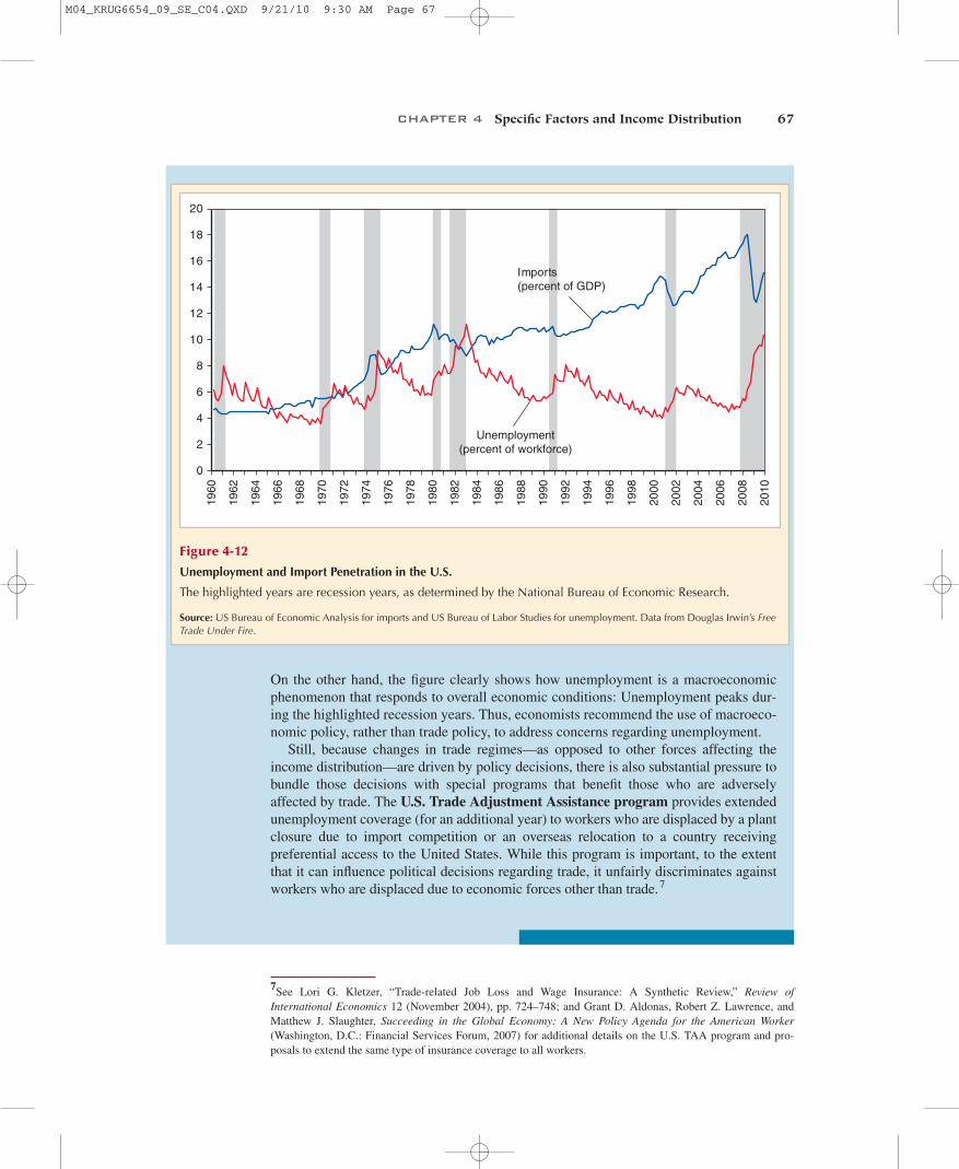
Figure 4-12 shows that, over the last 50 years in the United States, there is no obvi-ous correlation between the unemployment rate and imports (relative to U.S. GDP).
M04_KRUG6654_09_SE_C04.QXD 9/21/10 9:30 AM Page 66
CHAPTER 4 Specific Factors and Income Distribution 67
On the other hand, the figure clearly shows how unemployment is a macroeconomicphenomenon that responds to overall economic conditions: Unemployment peaks dur-ing the highlighted recession years. Thus, economists recommend the use of macroeco-nomic policy, rather than trade policy, to address concerns regarding unemployment.
Still, because changes in trade regimes—as opposed to other forces affecting theincome distribution—are driven by policy decisions, there is also substantial pressure tobundle those decisions with special programs that benefit those who are adverselyaffected by trade. The U.S. Trade Adjustment Assistance program provides extendedunemployment coverage (for an additional year) to workers who are displaced by a plantclosure due to import competition or an overseas relocation to a country receivingpreferential access to the United States. While this program is important, to the extentthat it can influence political decisions regarding trade, it unfairly discriminates againstworkers who are displaced due to economic forces other than trade.7
0
2
4
6
8
10
12
14
16
18
2019
60
1962
1964
1966
1968
1970
1972
1974
1976
1978
1980
1982
1984
1986
1988
1990
1992
1994
1996
1998
2000
2002
2004
2006
2008
2010
Imports(percent of GDP)
Unemployment(percent of workforce)
Figure 4-12
Unemployment and Import Penetration in the U.S.
The highlighted years are recession years, as determined by the National Bureau of Economic Research.
Source: US Bureau of Economic Analysis for imports and US Bureau of Labor Studies for unemployment. Data from Douglas Irwin’s FreeTrade Under Fire.
7See Lori G. Kletzer, “Trade-related Job Loss and Wage Insurance: A Synthetic Review,” Review ofInternational Economics 12 (November 2004), pp. 724–748; and Grant D. Aldonas, Robert Z. Lawrence, andMatthew J. Slaughter, Succeeding in the Global Economy: A New Policy Agenda for the American Worker(Washington, D.C.: Financial Services Forum, 2007) for additional details on the U.S. TAA program and pro-posals to extend the same type of insurance coverage to all workers.
M04_KRUG6654_09_SE_C04.QXD 9/21/10 9:30 AM Page 67
68 PART ONE International Trade Theory
Income Distribution and Trade PoliticsIt is easy to see why groups that lose from trade lobby their governments to restricttrade and protect their incomes. You might expect that those who gain from tradewould lobby as strongly as those who lose from it, but this is rarely the case. In theUnited States and most other countries, those who want trade limited are more effectivepolitically than those who want it extended. Typically, those who gain from trade inany particular product are a much less concentrated, informed, and organized groupthan those who lose.
A good example of this contrast between the two sides is the U.S. sugar industry. TheUnited States has limited imports of sugar for many years; over the past 25 years, the aver-age price of sugar in the U.S. market has been more than twice the average price on theworld market. Most estimates put the cost to U.S. consumers of this import limitation atabout $2 billion a year (according to the U.S. General Accounting Office)—that is, about$7 a year for every man, woman, and child. The gains to producers are much smaller,probably less than half as large.8
If producers and consumers were equally able to get their interests represented, thispolicy would never have been enacted. In absolute terms, however, each consumer suffersvery little. Seven dollars a year is not much; furthermore, most of the cost is hidden,because most sugar is consumed as an ingredient in other foods rather than purchaseddirectly. As a result, most consumers are unaware that the import quota even exists, letalone that it reduces their standard of living. Even if they were aware, $7 is not a largeenough sum to provoke people into organizing protests and writing letters to their congres-sional representatives.
The situation of the sugar producers (those who would lose from increased trade) isquite different. The higher profits from the import quota are highly concentrated in a smallnumber of producers. (Seventeen sugar cane farms generate more than half of the profitsfor the whole sugar cane industry.) Those producers are organized in trade associationsthat actively lobby on their members’ behalf, and make large campaign contributions.(The sugar cane and sugar beet political action committees contributed $3.3 million in the2006 election cycle.)
As one would expect, most of the gains from the sugar import restrictions go to thatsmall group of sugar cane farm owners and not to their employees. Of course, the traderestrictions do prevent job losses for those workers; but the consumer cost per jobsaved amounts to $826,000 per year, nearly 30 times the average pay of those workers.In addition, the sugar import restrictions also reduce employment in other sectors thatrely on large quantities of sugar in their production processes. In response to the highsugar prices in the United States, for example, candy-making firms have shifted theirproduction sites to Canada, where sugar prices are substantially lower. (There are nosugar farmers in Canada, and hence no political pressure for restrictions on sugarimports.)
As we will see in Chapters 9 through 12, the politics of import restriction in the sugar industry is an extreme example of a kind of political process that is common in internationaltrade. That world trade in general became steadily freer from 1945 to 1980 depended, as wewill see in Chapter 10, on a special set of circumstances that controlled what is probably aninherent political bias against international trade.
8See Chapter 3 of Douglas Irwin, Free Trade under Fire, 3rd edition (Princeton, NJ: Princeton University Press,2009) for a detailed description of the effects of sugar import restrictions in the United States.
M04_KRUG6654_09_SE_C04.QXD 9/21/10 9:30 AM Page 68
CHAPTER 4 Specific Factors and Income Distribution 69
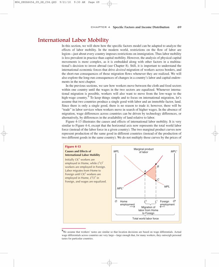
International Labor MobilityIn this section, we will show how the specific factors model can be adapted to analyze theeffects of labor mobility. In the modern world, restrictions on the flow of labor arelegion—just about every country imposes restrictions on immigration. Thus labor mobilityis less prevalent in practice than capital mobility. However, the analysis of physical capitalmovements is more complex, as it is embedded along with other factors in a multina-tional’s decision to invest abroad (see Chapter 8). Still, it is important to understand theinternational economic forces that drive desired migration of workers across borders, andthe short-run consequences of those migration flows whenever they are realized. We willalso explore the long-run consequences of changes in a country’s labor and capital endow-ments in the next chapter.
In the previous sections, we saw how workers move between the cloth and food sectorswithin one country until the wages in the two sectors are equalized. Whenever interna-tional migration is possible, workers will also want to move from the low-wage to thehigh-wage country.9 To keep things simple and to focus on international migration, let’sassume that two countries produce a single good with labor and an immobile factor, land.Since there is only a single good, there is no reason to trade it; however, there will be“trade” in labor services when workers move in search of higher wages. In the absence ofmigration, wage differences across countries can be driven by technology differences, oralternatively, by differences in the availability of land relative to labor.
Figure 4-13 illustrates the causes and effects of international labor mobility. It is verysimilar to Figure 4-4, except that the horizontal axis now represents the total world laborforce (instead of the labor force in a given country). The two marginal product curves nowrepresent production of the same good in different countries (instead of the production oftwo different goods in the same country). We do not multiply those curves by the prices of
Marginal productof labor
Home employment
Total world labor force
Foreign employment
L2 L1
Migration oflabor from Home
to Foreign
A
B
C
MPL*MPL
O*O
MPL MPL*
Figure 4-13
Causes and Effects ofInternational Labor Mobility
Initially workers are employed in Home, while workers are employed in Foreign.Labor migrates from Home toForeign until workers areemployed in Home, inForeign, and wages are equalized.
L2O*OL2
L1O*OL1
9We assume that workers’ tastes are similar so that location decisions are based on wage differentials. Actualwage differentials across countries are very large—large enough that, for many workers, they outweigh personaltastes for particular countries.
M04_KRUG6654_09_SE_C04.QXD 9/21/10 9:30 AM Page 69
70 PART ONE International Trade Theory
the good; instead we assume that the wages measured on the vertical axis represent realwages (the wage divided by the price of the unique good in each country). Initially, weassume that there are workers in Home and workers in Foreign. Given thoseemployment levels, technology and land endowment differences are such that real wagesare higher in Foreign (point B) than in Home (point C).
Now suppose that workers are able to move between these two countries. Workers willmove from Home to Foreign. This movement will reduce the Home labor force and thusraise the real wage in Home, while increasing the labor force and reducing the real wage inForeign. If there are no obstacles to labor movement, this process will continue until thereal wage rates are equalized. The eventual distribution of the world’s labor force will beone with workers in Home and workers in Foreign (point A).
Three points should be noted about this redistribution of the world’s labor force.
1. It leads to a convergence of real wage rates. Real wages rise in Home and fall in Foreign.2. It increases the world’s output as a whole. Foreign’s output rises by the area under its mar-
ginal product curve from to , while Home’s falls by the corresponding area under itsmarginal product curve. (See appendix for details.) We see from the figure that Foreign’sgain is larger than Home’s loss, by an amount equal to the colored area ABC in the figure.
3. Despite this gain, some people are hurt by the change. Those who would originallyhave worked in Home receive higher real wages, but those who would originally haveworked in Foreign receive lower real wages. Landowners in Foreign benefit from thelarger labor supply, but landowners in Home are made worse off.
As in the case of the gains from international trade, then, international labor mobility,while allowing everyone to be made better off in principle, leaves some groups worse off inpractice. This main result would not change in a more complex model where countries pro-duce and trade different goods, so long as some factors of production are immobile in theshort run. However, we will see in the following chapter that this result need not hold in thelong run, when all factors are mobile across sectors. We will see how changes in a country’slabor endowment, so long as the country is integrated into world markets through trade, canleave the welfare of all factors unchanged. This has very important implications for immi-gration in the long run, and has been shown to be empirically relevant in cases where coun-tries experience large immigration increases.
L2L1
L2O*OL2
L1O*OL1
Case Study
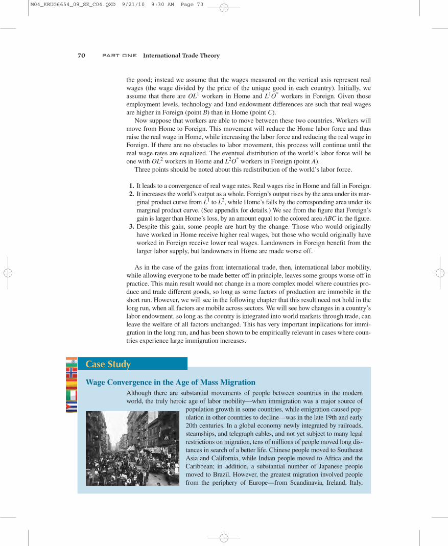
Wage Convergence in the Age of Mass MigrationAlthough there are substantial movements of people between countries in the modernworld, the truly heroic age of labor mobility—when immigration was a major source of
population growth in some countries, while emigration caused pop-ulation in other countries to decline—was in the late 19th and early20th centuries. In a global economy newly integrated by railroads,steamships, and telegraph cables, and not yet subject to many legalrestrictions on migration, tens of millions of people moved long dis-tances in search of a better life. Chinese people moved to SoutheastAsia and California, while Indian people moved to Africa and theCaribbean; in addition, a substantial number of Japanese peoplemoved to Brazil. However, the greatest migration involved peoplefrom the periphery of Europe—from Scandinavia, Ireland, Italy,
M04_KRUG6654_09_SE_C04.QXD 9/21/10 9:30 AM Page 70
CHAPTER 4 Specific Factors and Income Distribution 71
and Eastern Europe—who moved to places where land was abundant and wages werehigh: the United States, Canada, Argentina, and Australia.
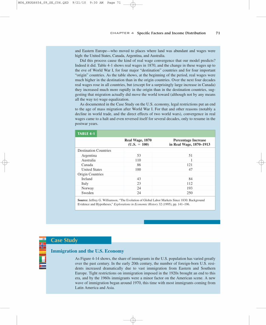
Did this process cause the kind of real wage convergence that our model predicts?Indeed it did. Table 4-1 shows real wages in 1870, and the change in these wages up tothe eve of World War I, for four major “destination” countries and for four important“origin” countries. As the table shows, at the beginning of the period, real wages weremuch higher in the destination than in the origin countries. Over the next four decadesreal wages rose in all countries, but (except for a surprisingly large increase in Canada)they increased much more rapidly in the origin than in the destination countries, sug-gesting that migration actually did move the world toward (although not by any meansall the way to) wage equalization.
As documented in the Case Study on the U.S. economy, legal restrictions put an endto the age of mass migration after World War I. For that and other reasons (notably adecline in world trade, and the direct effects of two world wars), convergence in realwages came to a halt and even reversed itself for several decades, only to resume in thepostwar years.
TABLE 4-1
Real Wage, 1870(U.S. = 100)
Percentage Increase in Real Wage, 1870–1913
Destination CountriesArgentina 53 51Australia 110 1Canada 86 121United States 100 47
Origin CountriesIreland 43 84Italy 23 112Norway 24 193Sweden 24 250
Source: Jeffrey G. Williamson, “The Evolution of Global Labor Markets Since 1830: BackgroundEvidence and Hypotheses,” Explorations in Economic History 32 (1995), pp. 141–196.
Case Study
Immigration and the U.S. Economy
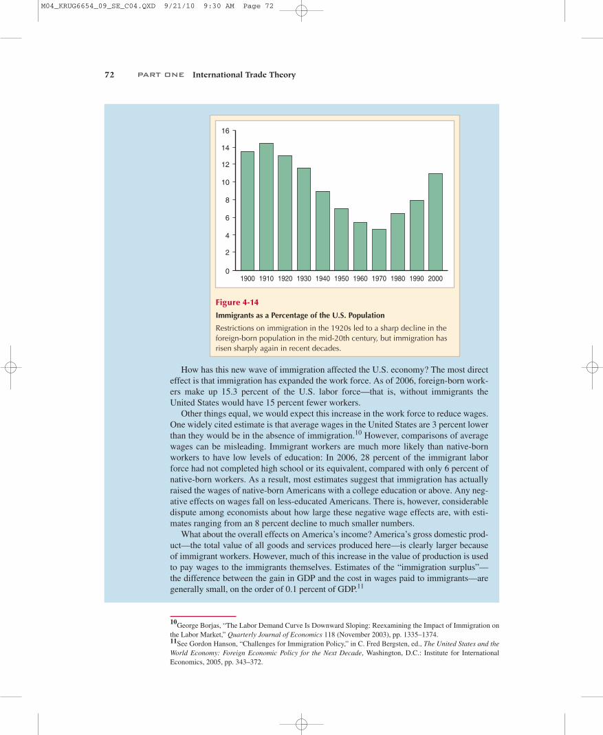
As Figure 4-14 shows, the share of immigrants in the U.S. population has varied greatlyover the past century. In the early 20th century, the number of foreign-born U.S. resi-dents increased dramatically due to vast immigration from Eastern and SouthernEurope. Tight restrictions on immigration imposed in the 1920s brought an end to thisera, and by the 1960s immigrants were a minor factor on the American scene. A newwave of immigration began around 1970, this time with most immigrants coming fromLatin America and Asia.
M04_KRUG6654_09_SE_C04.QXD 9/21/10 9:30 AM Page 71
72 PART ONE International Trade Theory
How has this new wave of immigration affected the U.S. economy? The most directeffect is that immigration has expanded the work force. As of 2006, foreign-born work-ers make up 15.3 percent of the U.S. labor force—that is, without immigrants theUnited States would have 15 percent fewer workers.
Other things equal, we would expect this increase in the work force to reduce wages.One widely cited estimate is that average wages in the United States are 3 percent lowerthan they would be in the absence of immigration.10 However, comparisons of averagewages can be misleading. Immigrant workers are much more likely than native-bornworkers to have low levels of education: In 2006, 28 percent of the immigrant laborforce had not completed high school or its equivalent, compared with only 6 percent ofnative-born workers. As a result, most estimates suggest that immigration has actuallyraised the wages of native-born Americans with a college education or above. Any neg-ative effects on wages fall on less-educated Americans. There is, however, considerabledispute among economists about how large these negative wage effects are, with esti-mates ranging from an 8 percent decline to much smaller numbers.
What about the overall effects on America’s income? America’s gross domestic prod-uct—the total value of all goods and services produced here—is clearly larger becauseof immigrant workers. However, much of this increase in the value of production is usedto pay wages to the immigrants themselves. Estimates of the “immigration surplus”—the difference between the gain in GDP and the cost in wages paid to immigrants—aregenerally small, on the order of 0.1 percent of GDP.11
12
6
8
10
4
2
01900 1910 1920 1930 1940 1950 1960 1970 1980 1990 2000
14
16
Figure 4-14
Immigrants as a Percentage of the U.S. Population
Restrictions on immigration in the 1920s led to a sharp decline in theforeign-born population in the mid-20th century, but immigration hasrisen sharply again in recent decades.
10George Borjas, “The Labor Demand Curve Is Downward Sloping: Reexamining the Impact of Immigration onthe Labor Market,” Quarterly Journal of Economics 118 (November 2003), pp. 1335–1374.11See Gordon Hanson, “Challenges for Immigration Policy,” in C. Fred Bergsten, ed., The United States and theWorld Economy: Foreign Economic Policy for the Next Decade, Washington, D.C.: Institute for InternationalEconomics, 2005, pp. 343–372.
M04_KRUG6654_09_SE_C04.QXD 9/21/10 9:30 AM Page 72
CHAPTER 4 Specific Factors and Income Distribution 73
SUMMARY
1. International trade often has strong effects on the distribution of income within coun-tries, so that it often produces losers as well as winners. Income distribution effectsarise for two reasons: Factors of production cannot move instantaneously and cost-lessly from one industry to another, and changes in an economy’s output mix havedifferential effects on the demand for different factors of production.
2. A useful model of income distribution effects of international trade is the specific fac-tors model, which allows for a distinction between general-purpose factors that canmove between sectors and factors that are specific to particular uses. In this model, dif-ferences in resources can cause countries to have different relative supply curves, andthus cause international trade.
3. In the specific factors model, factors specific to export sectors in each country gainfrom trade, while factors specific to import-competing sectors lose. Mobile factors thatcan work in either sector may either gain or lose.
4. Trade nonetheless produces overall gains in the limited sense that those who gain couldin principle compensate those who lose while still remaining better off than before.
5. Most economists do not regard the effects of international trade on income distributiona good reason to limit this trade. In its distributional effects, trade is no different frommany other forms of economic change, which are not normally regulated. Furthermore,economists would prefer to address the problem of income distribution directly, ratherthan by interfering with trade flows.
6. Nonetheless, in the actual politics of trade policy, income distribution is of crucialimportance. This is true in particular because those who lose from trade are usually amuch more informed, cohesive, and organized group than those who gain.
7. International factor movements can sometimes substitute for trade, so it is not surpris-ing that international migration of labor is similar in its causes and effects to interna-tional trade. Labor moves from countries where it is abundant to countries where it isscarce. This movement raises total world output, but it also generates strong incomedistribution effects, so that some groups are hurt as a result.
There’s one more complication in assessing the economic effects of immigration:the effects on tax revenue and government spending. On one side, immigrants paytaxes, helping cover the cost of government. On the other side, they impose costs on thegovernment, because their cars need roads to drive on, their children need schools tostudy in, and so on. Because many immigrants earn low wages and hence pay lowtaxes, some estimates suggest that immigrants cost more in additional spending thanthey pay in. However, estimates of the net fiscal cost, like estimates of the net economiceffects, are small, again on the order of 0.1 percent of GDP.
Immigration is, of course, an extremely contentious political issue. The economicsof immigration, however, probably doesn’t explain this contentiousness. Instead, it maybe helpful to recall what the Swiss author Max Frisch once said about the effects of im-migration into his own country, which at one point relied heavily on workers from othercountries: “We asked for labor, but people came.” And it’s the fact that immigrants arepeople that makes the immigration issue so difficult.
M04_KRUG6654_09_SE_C04.QXD 9/21/10 9:30 AM Page 73
74 PART ONE International Trade Theory
KEY TERMS
budget constraint, p. 64diminishing returns, p. 53marginal product of labor, p. 53mobile factor, p. 51
production function, p. 52production possibility
frontier, p. 53specific factor, p. 51
specific factors model, p. 51U.S. Trade Adjustment
Assistance program, p. 67
PROBLEMS
1. In 1986, the price of oil on world markets dropped sharply. Since the United States isan oil-importing country, this was widely regarded as good for the U.S. economy. Yetin Texas and Louisiana, 1986 was a year of economic decline. Why?
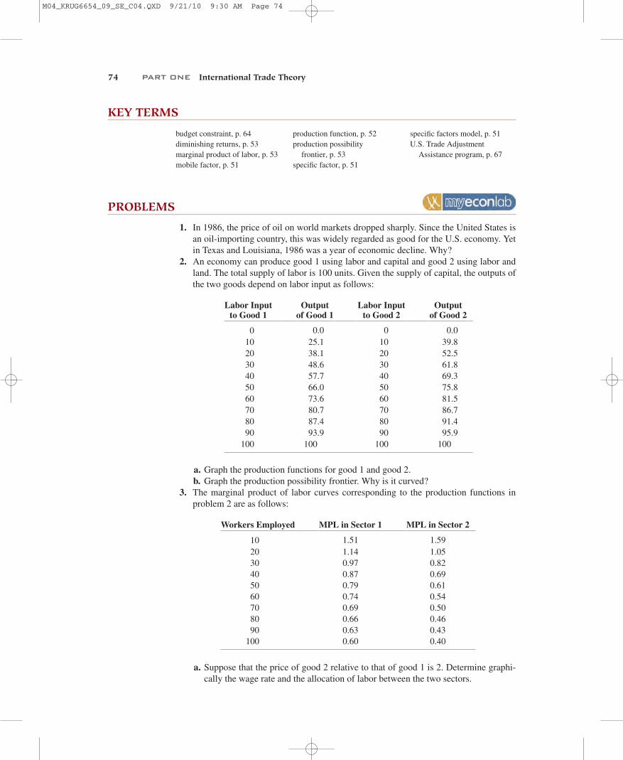
2. An economy can produce good 1 using labor and capital and good 2 using labor andland. The total supply of labor is 100 units. Given the supply of capital, the outputs ofthe two goods depend on labor input as follows:
Labor Input to Good 1
Output of Good 1
Labor Input to Good 2
Output of Good 2
0 0.0 0 0.010 25.1 10 39.820 38.1 20 52.530 48.6 30 61.840 57.7 40 69.350 66.0 50 75.860 73.6 60 81.570 80.7 70 86.780 87.4 80 91.490 93.9 90 95.9
100 100 100 100
a. Graph the production functions for good 1 and good 2.b. Graph the production possibility frontier. Why is it curved?
3. The marginal product of labor curves corresponding to the production functions inproblem 2 are as follows:
Workers Employed MPL in Sector 1 MPL in Sector 2
10 1.51 1.5920 1.14 1.0530 0.97 0.8240 0.87 0.6950 0.79 0.6160 0.74 0.5470 0.69 0.5080 0.66 0.4690 0.63 0.43
100 0.60 0.40
a. Suppose that the price of good 2 relative to that of good 1 is 2. Determine graphi-cally the wage rate and the allocation of labor between the two sectors.
M04_KRUG6654_09_SE_C04.QXD 9/21/10 9:30 AM Page 74
CHAPTER 4 Specific Factors and Income Distribution 75
b. Using the graph drawn for problem 2, determine the output of each sector. Thenconfirm graphically that the slope of the production possibility frontier at that pointequals the relative price.
c. Suppose that the relative price of good 2 falls to 1. Repeat (a) and (b).d. Calculate the effects of the price change from 2 to 1 on the income of the specific
factors in sectors 1 and 2.4. Consider two countries (Home and Foreign) that produce goods 1 (with labor and capi-
tal) and 2 (with labor and land) according to the production functions described in prob-lems 2 and 3. Initially, both countries have the same supply of labor (100 units each),capital, and land. The capital stock in Home then grows. This change shifts out both theproduction curve for good 1 as a function of labor employed (described in problem 2)and the associated marginal product of labor curve (described in problem 3). Nothinghappens to the production and marginal product curves for good 2.a. Show how the increase in the supply of capital for Home affects its production
possibility frontier.b. On the same graph, draw the relative supply curve for both the Home and the
Foreign economy.c. If those two economies open up to trade, what will be the pattern of trade (i.e.,
which country exports which good)?d. Describe how opening up to trade affects all three factors (labor, capital, land) in
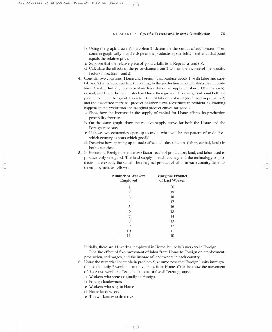
both countries.5. In Home and Foreign there are two factors each of production, land, and labor used to
produce only one good. The land supply in each country and the technology of pro-duction are exactly the same. The marginal product of labor in each country dependson employment as follows:
Number of Workers Employed
Marginal Product of Last Worker
1 202 193 184 175 166 157 148 139 12
10 1111 10
Initially, there are 11 workers employed in Home, but only 3 workers in Foreign.Find the effect of free movement of labor from Home to Foreign on employment,
production, real wages, and the income of landowners in each country.6. Using the numerical example in problem 5, assume now that Foreign limits immigra-
tion so that only 2 workers can move there from Home. Calculate how the movementof these two workers affects the income of five different groups:a. Workers who were originally in Foreignb. Foreign landownersc. Workers who stay in Homed. Home landownerse. The workers who do move
M04_KRUG6654_09_SE_C04.QXD 9/21/10 9:30 AM Page 75
7. Studies of the effects of immigration into the United States from Mexico tend to findthat the big winners are the immigrants themselves. Explain this result in terms of theexample in the question above. How might things change if the border were open,with no restrictions on immigration?
FURTHER READINGS
Avinash Dixit and Victor Norman. Theory of International Trade. Cambridge: Cambridge UniversityPress, 1980. The problem of establishing gains from trade when some people may be made worseoff has been the subject of a long debate. Dixit and Norman show it is always possible in principlefor a country’s government to use taxes and subsidies to redistribute income in such a way thateveryone is better off with free trade than with no trade.
Douglas A. Irwin, Free Trade under Fire, 3rd edition. Princeton, NJ: Princeton University Press,2009. An accessible book that provides numerous details and supporting data for the argumentthat freer trade generates overall welfare gains. Chapter 4 discusses the connection betweentrade and unemployment in detail (an issue that was briefly discussed in this chapter).
Charles P. Kindleberger. Europe’s Postwar Growth: The Role of Labor Supply. Cambridge: HarvardUniversity Press, 1967. A good account of the role of labor migration during its height in Europe.
Robert A. Mundell. “International Trade and Factor Mobility.” American Economic Review 47 (1957),pp. 321–335. The paper that first laid out the argument that trade and factor movement can substi-tute for each other.
Michael Mussa. “Tariffs and the Distribution of Income: The Importance of Factor Specificity,Substitutability, and Intensity in the Short and Long Run.” Journal of Political Economy 82(1974), pp. 1191–1204. An extension of the specific factors model that relates it to the factorproportions model of Chapter 5.
J. Peter Neary. “Short-Run Capital Specificity and the Pure Theory of International Trade.”Economic Journal 88 (1978), pp. 488–510. A further treatment of the specific factors model thatstresses how differing assumptions about mobility of factors between sectors affect the model’sconclusions.
Mancur Olson. The Logic of Collective Action. Cambridge: Harvard University Press, 1965. Ahighly influential book that argues the proposition that in practice, government policies favorsmall, concentrated groups over large ones.
David Ricardo. The Principles of Political Economy and Taxation. Homewood, IL: Irwin, 1963.While Ricardo’s Principles emphasizes the national gains from trade at one point, elsewhere inhis book the conflict of interest between landowners and capitalists is a central issue.
76 PART ONE International Trade Theory
M04_KRUG6654_09_SE_C04.QXD 9/21/10 9:30 AM Page 76
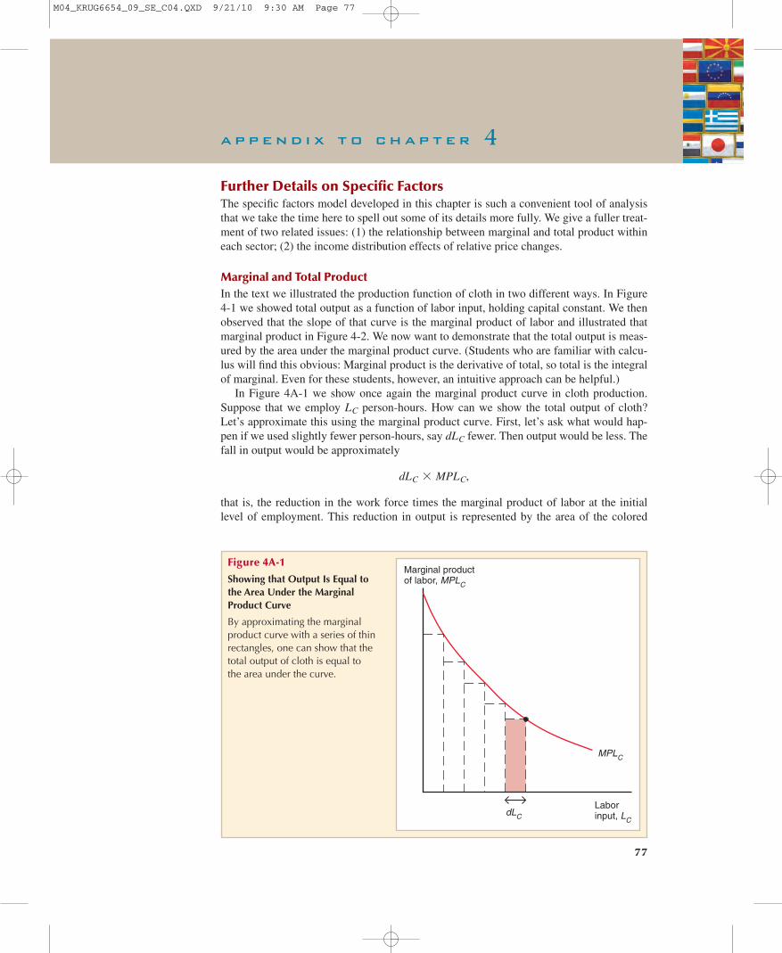
77
a p p e n d i x t o c h a p t e r 4
Further Details on Specific FactorsThe specific factors model developed in this chapter is such a convenient tool of analysisthat we take the time here to spell out some of its details more fully. We give a fuller treat-ment of two related issues: (1) the relationship between marginal and total product withineach sector; (2) the income distribution effects of relative price changes.
Marginal and Total ProductIn the text we illustrated the production function of cloth in two different ways. In Figure4-1 we showed total output as a function of labor input, holding capital constant. We thenobserved that the slope of that curve is the marginal product of labor and illustrated thatmarginal product in Figure 4-2. We now want to demonstrate that the total output is meas-ured by the area under the marginal product curve. (Students who are familiar with calcu-lus will find this obvious: Marginal product is the derivative of total, so total is the integralof marginal. Even for these students, however, an intuitive approach can be helpful.)
In Figure 4A-1 we show once again the marginal product curve in cloth production.Suppose that we employ person-hours. How can we show the total output of cloth?Let’s approximate this using the marginal product curve. First, let’s ask what would hap-pen if we used slightly fewer person-hours, say fewer. Then output would be less. Thefall in output would be approximately
that is, the reduction in the work force times the marginal product of labor at the initiallevel of employment. This reduction in output is represented by the area of the colored
dLC * MPLC,
dLC
LC
Marginal productof labor, MPLC
Labor input, LC
dLC
MPLC
Figure 4A-1
Showing that Output Is Equal tothe Area Under the MarginalProduct Curve
By approximating the marginalproduct curve with a series of thinrectangles, one can show that thetotal output of cloth is equal tothe area under the curve.
M04_KRUG6654_09_SE_C04.QXD 9/21/10 9:30 AM Page 77
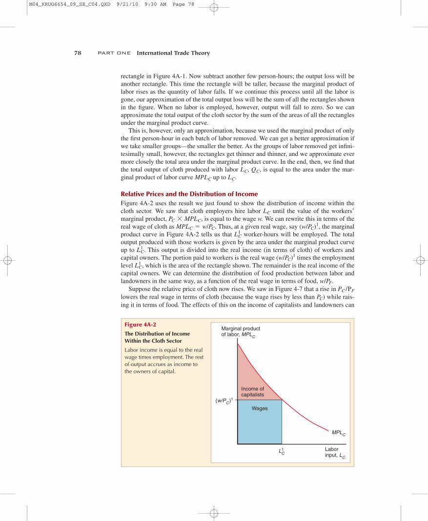
rectangle in Figure 4A-1. Now subtract another few person-hours; the output loss will beanother rectangle. This time the rectangle will be taller, because the marginal product oflabor rises as the quantity of labor falls. If we continue this process until all the labor isgone, our approximation of the total output loss will be the sum of all the rectangles shownin the figure. When no labor is employed, however, output will fall to zero. So we canapproximate the total output of the cloth sector by the sum of the areas of all the rectanglesunder the marginal product curve.
This is, however, only an approximation, because we used the marginal product of onlythe first person-hour in each batch of labor removed. We can get a better approximation ifwe take smaller groups—the smaller the better. As the groups of labor removed get infini-tesimally small, however, the rectangles get thinner and thinner, and we approximate evermore closely the total area under the marginal product curve. In the end, then, we find thatthe total output of cloth produced with labor , , is equal to the area under the mar-ginal product of labor curve up to .
Relative Prices and the Distribution of IncomeFigure 4A-2 uses the result we just found to show the distribution of income within thecloth sector. We saw that cloth employers hire labor until the value of the workers’marginal product, , is equal to the wage w. We can rewrite this in terms of thereal wage of cloth as . Thus, at a given real wage, say , the marginalproduct curve in Figure 4A-2 tells us that worker-hours will be employed. The totaloutput produced with those workers is given by the area under the marginal product curveup to . This output is divided into the real income (in terms of cloth) of workers andcapital owners. The portion paid to workers is the real wage times the employmentlevel , which is the area of the rectangle shown. The remainder is the real income of thecapital owners. We can determine the distribution of food production between labor andlandowners in the same way, as a function of the real wage in terms of food, .
Suppose the relative price of cloth now rises. We saw in Figure 4-7 that a rise in lowers the real wage in terms of cloth (because the wage rises by less than ) while rais-ing it in terms of food. The effects of this on the income of capitalists and landowners can
PC
PC /PF
w/PF
LC1
(w/PC)1LC
1
LC1
(w/PC)1MPLC = w/PC
PC * MPLC
LC
LCMPLC
QCLC
78 PART ONE International Trade Theory
Marginal productof labor, MPLC
Labor input, LC
MPLC
(w/PC )1
Income of capitalists
Wages
L1C
Figure 4A-2
The Distribution of IncomeWithin the Cloth Sector
Labor income is equal to the realwage times employment. The restof output accrues as income tothe owners of capital.
M04_KRUG6654_09_SE_C04.QXD 9/21/10 9:30 AM Page 78
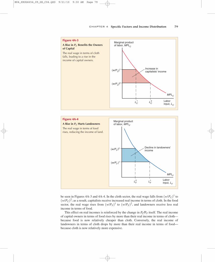
CHAPTER 4 Specific Factors and Income Distribution 79
Marginal productof labor, MPLC
Labor input, LC
Increase incapitalists’ income
(w/PC)2
(w/PC)1
MPLC
LC2LC
1
Figure 4A-3
A Rise in Benefits the Ownersof Capital
The real wage in terms of clothfalls, leading to a rise in theincome of capital owners.
PC
Marginal productof labor, MPLF
Labor input, LF
Decline in landowners’income(w/PF )2
(w/PF )1
MPLF
LF2 LF
1
Figure 4A-4
A Rise in Hurts Landowners
The real wage in terms of foodrises, reducing the income of land.
PC
be seen in Figures 4A-3 and 4A-4. In the cloth sector, the real wage falls from to; as a result, capitalists receive increased real income in terms of cloth. In the food
sector, the real wage rises from to , and landowners receive less realincome in terms of food.
This effect on real incomes is reinforced by the change in itself. The real incomeof capital owners in terms of food rises by more than their real income in terms of cloth—because food is now relatively cheaper than cloth. Conversely, the real income oflandowners in terms of cloth drops by more than their real income in terms of food—because cloth is now relatively more expensive.
PC/PF
1w/PF221w/PF2
11w/PC2
21w/PC2
1
M04_KRUG6654_09_SE_C04.QXD 9/21/10 9:30 AM Page 79