Embed Size (px)
Citation preview
2003
Special Studiesin
Federal Tax Statistics
Compiled and Edited byJames Dalton and Beth Kilss*Statistics of Income Division
Internal Revenue Service
Selected Papers Given in 2003at the Annual Meetings of the
American Statistical Association
*Prepared under the direction of Tom Petska, Director, Statistics of Income
�
1 ARE THE RICH GETTING RICHER AND THE POOR GETTING POORER?
Measuring Household Income Inequality Using the CPS, by Edward J. Welniak ...........................3
An Analysis of the Distribution of Individual Income and Taxes, 1979-2001, byMichael Strudler, Tom Petska, and Ryan Petska ......................................................................13
The Distribution of Household Income: Two Decades of Change, by Roberton Williams ............23
Comments on Papers by Welniak; Strudler, Petska, and Petska; and Williams,by Eric J. Toder .........................................................................................................................37
2 RECENT DEVELOPMENT IN SURVEY METHODS
Comparing Scoring Systems From Cluster Analysis and Discriminant Analysis Using RandomSamples, by William Wong and Chih-Chin Ho ..........................................................................43
3 NEW DEVELOPMENTS IN TAX STATISTICS AND ADMINISTRATIVE RECORDS
Accumulation and Distributions of Retirement Assets, 1996-2000: Results From a MatchedFile of Tax Returns and Information Returns, by Peter Sailer, Kurt S. Gurka, andSarah Holden ............................................................................................................................53
The Effects of Tax Reform on the Structure of U.S. Business, by Ellen Legel, Kelly Bennett,and Michael Parisi ....................................................................................................................63
Statistical Information Services at IRS: Improving Dissemination of Data and Satisfying theCustomer, by Beth Kilss and David Jordan ...............................................................................71
Special Studies in Federal Tax Statistics2003
CONTENTS
Preface
-v-
..................................................................................................................................... iii
PAGE
�
��
IRS Seeks To Develop New Web-Based Measurement Indicators for IRS.gov, byDiane M. Dixon ........................................................................................................................ 79
Recent Efforts To Maximize Benefits From the Statistics of Income Advisory Panel, byTom Petska and Beth Kilss ....................................................................................................... 87
4 SURVEY NONRESPONSE AND IMPUTATION
Regulatory Exemptions and Item Nonresponse, by Paul B. McMahon ........................................ 97
INDEX OF IRS METHODOLOGY REPORTS ON STATISTICAL USES OF ADMINISTRATIVE RECORDS .......... 107
PAGE
-vi-
CONTENTS
�

�
1
Are the Rich Getting Richerand the Poor Getting Poorer?
WelniakStrudler Petska Petska
WilliamsToder
� �
- 3 -
Measuring Household Income Inequality Using the CPSEdward J. Welniak, U.S. Census Bureau
Disclaimer: This paper reports the results of researchand analysis undertaken by Census Bureau staff. It hasundergone a Census Bureau review more limited in scopethan that given to official Census Bureau publications.This report is released to inform interested parties ofongoing research and to encourage discussion of workin progress.
� Introduction
This paper examines the use of the Current Popula-tion Survey (CPS) to measure income inequality. It be-gins with a brief overview of the CPS followed by apresentation of how three income inequality measurestrack over time using CPS household data. It goes on toexamine topcoding issues associated with CPS incomedata, how CPS topcoding affects the measurement ofincome inequality, and concludes with a discussion ofCPS income data quality issues.
� An Overview of the CPS
The CPS is a national random household samplesurvey conducted monthly by the Census Bureau forthe Bureau of Labor Statistics. The monthly samplesize for the CPS is about 78,000 households.1 The sur-vey has been conducted for more than 50 years.
The CPS is the primary source of information onthe labor force characteristics of the U.S. population.The sample is scientifically selected to represent the ci-vilian noninstitutional population. Respondents are in-terviewed to obtain information about the employmentstatus of each member of the household 15 years of ageand older.
Estimates obtained from the CPS include employ-ment, unemployment, earnings, hours of work, and otherindicators. They are available by a variety of demographiccharacteristics including age, sex, race, ethnicity, mari-tal status, and educational attainment. They are also avail-able by occupation, industry, and class of worker.
Supplemental questions to produce estimates on a vari-ety of topics, including school enrollment, income, previ-ous work experience, health, employee benefits, andwork schedules, are also often added to the regular CPSquestionnaire.
One of the CPS�s most widely used supplements isthe Annual Social and Economic Supplement (ASEC).2The ASEC is the source of annual income, official pov-erty, and health coverage statistics for the U. S. TheASEC has been used to compile annual income sum-mary measures for families and people since 1947 andfor households since 1967. Households have become amore comprehensive unit of analysis over time due tochanging living patterns (a smaller percentage of peoplecurrently live in family situations than 50 years ago).Household income data is constructed from income in-formation collected about the civilian, noninstitutionalizedpopulation 15 years old and over.3 Households excludepeople living in group quarters.
Income collected in the CPS ASEC is defined asmoney income received on a regular basis, before de-ductions for taxes and other expenses, and does not in-clude lump-sum payments or capital gains. It includeswages and salary, self-employment (net after expenses),unemployment compensation, worker�s compensation,Social Security, Supplemental Security Income, cashpublic assistance, veterans� payments, survivor benefits,pension or retirement income, interest, dividends, rents,royalties, estates, trusts, educational assistance, alimony,child support, assistance from outside the household, andother miscellaneous money income received on a regu-lar basis.
The income data collected in the CPS ASEC havebecome more detailed over time. In 1967, data werecollected on eight sources of income. The 1967 sourcesincluded wages and salaries, which were one of the twooriginal income sources asked in 1947, two sources ofself-employment income (farm and nonfarm, which wereadded in 1950), and five additional sources added in 1967:
- 4 -
WELNIAK
Social Security; interest, dividends, estate, trust, or rent;public assistance or welfare; unemployment compensa-tion, worker�s compensation, government employee pen-sions, or veterans payments; and private pensions, an-nuities, alimony, royalties, or regular contributions frompeople not living in the household. The number of in-come sources continued to expand until 1979 when theCPS ASEC allowed for the identification of over 50 in-come sources while recording up to 27 income values.The income sources have remained unchanged since 1979(see Welniak for a complete discussion of the evolutionof the CPS ASEC questionnaire and processing system).
In addition to an increasing number of incomesources collected in the CPS ASEC, the values recordedfor these sources also increased. In 1967, the format ofthe CPS questionnaire allowed for the recording ofamounts up to $9,999 for each of the eight incomesources. In 1970, the format of the questionnaire changedallowing the recording limits to increase to $99,999 forsix of the eight income sources (wages and salaries; farmself-employment; nonfarm self-employment; interest,dividends, estate, trust, or rent; unemployment compen-sation, worker�s compensation, government employeepensions, or veterans payments; and private pensions,annuities, alimony, royalties, or regular contributions frompeople not living in the household). In 1979, the ques-tionnaire allowed the recording of up to $99,999 for 23income sources.4 In 1985, the limit for recording earn-ings from longest job increased to $299,999. The finalrecording limit increase occurred in 1993 when each ofthe four earned income sources allowed the recordingof amounts to $9,999,999.
� Measuring Household Income Inequality
Several measures of income inequality are availablefor analysis. Two important properties an inequalitymeasure should possess are scale invariance and theprinciple of transfers. An inequality measure is said tobe scale invariant if the measure does not change whena constant is added to all income values in the distribu-tion. An inequality measure possesses the principle oftransfers if the measure rises (falls) when income is trans-ferred from the poorer household to a richer one (orvice versa).
This paper examines the changes in three measuresof household income inequality that possess these quali-ties: the Gini Coefficient, the Mean Logarithmic Devia-tion of Income (MLD), and the Atkinson Index.
The Gini index is a measure of income concentra-tion derived from the Lorenz Curve. The Lorenz Curveis obtained by plotting the cumulative percent of units onthe X-axis against the cumulative percent of aggregateincome accounted for by these units on the Y-axis. Adiagonal line from 0 percent to 100 percent would repre-sent the Lorenz Curve if all units had exactly the sameincome. Lorenz Curves plotted from actual data typicallyfall below the diagonal. The Gini index is the proportionof the total area below the diagonal that is between thediagonal and the Lorenz Curve. Thus, the Gini indexranges from 0 (perfect equality) to 1 (perfect inequality).
The Atkinson measure of inequality takes a currentincome distribution and translates it into a social welfarefunction. The measure is expressed as a ratio of thecurrent welfare function to a welfare function of equallydistributed income. The Atkinson measure incorporatesa parameter, e, which allows the user to quantify anaversion to inequality. The greater the e value, the moreaversion there is to inequality. The value of e rangesbetween 0 and 1, with 1 indicating maximum inequalityaversion with emphasis on the lower end of the incomedistribution.
The MLD measures the average ratio of the log ofthe population mean to each observation. The MLD be-longs to the Generalized Entropy family. It can be used tomeasure both within and between group income inequality.
� Historical Perspective on Household IncomeInequality
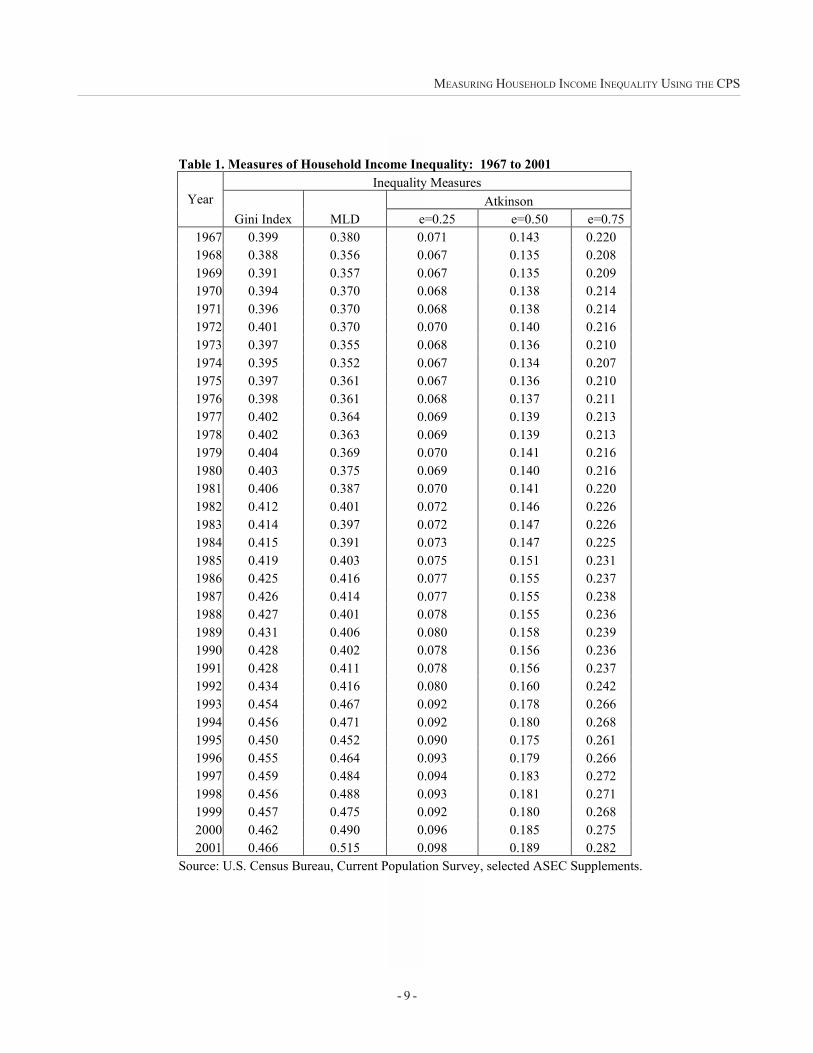
Each of the inequality measures displayed in Table1 was derived from the Census Bureau�s internal datafile. They show an increase in income inequality be-tween 1967 and 2001, to varying degrees: the Gini indexincreased 17 percent, the MLD 36 percent, and theAtkinson increased between 28 percent (e=0.75) and38 percent (e=0.25).5 Between 1967 and 1980, the Giniindex was relatively unchanged. The 1980 MLD andAtkinson measures were at or slightly below their 1967
- 5 -
MEASURING HOUSEHOLD INCOME INEQUALITY USING THE CPS
levels. Each of these measures was at or near its all-time lows by 1974 and was beginning to show signs ofincreasing. In 1974, the Gini was already above its all-time low set in 1968. By 1982, all of these measureswere at or above their 1967 levels and were increasing.
Most of these measures showed growth in incomeinequality through the late 1980�s. By 1989, the Gini andAtkinson measures were measuring income inequalityat levels comparable to their all-time highs. The Giniwas 8 percent higher than in 1967; the Atkinson with itsaversion parameter set to be more sensitive to changesin the upper end of the income distribution (e=0.25) was13 percent higher; the Atkinson with a midlevel inequal-ity aversion parameter (e=0.5) was 10 percent higher;the Atkinson with an inequality aversion parameter moresensitive to changes in the low end of the income distri-bution (e=0.75) was 9 percent higher; and the MLD was7 percent higher.6
There appeared to be little change in income inequal-ity between 1989 and 1991.7 Each of the measuresshowed growth in inequality between 1991 and 1993,though it is hard to quantify the growth because of sur-vey methodology changes that took place in 1993. In1994, the CPS ASEC introduced computer-assisted per-sonal interviewing and increased the recording levels forearnings to $1 million as well as increasing the recodinglevels for other income sources. Ryscavage (1995) foundthat as much as one-half of the growth in inequality be-tween 1992 and 1993 may have been the result of thesemethodological changes. Since 1993, each of the mea-sures has shown periods of fluctuation, culminating in anincrease in income inequality by 2001.
� Income Topcoding and Inequality Measurement
This section will examine the impact that incomerecording limits had on the measurement of income in-equality. Discussion will focus on the changes to theCPS ASEC questionnaire in 1970, 1979, 1985, and 1993and also the topcoding limits place on the public-use file.
As discussed earlier, the CPS ASEC has undergoneseveral changes with regard to changing income ques-tions and income recording and processing limits. In1970, income-recording limits increased to $99,999. This
change affected 12,505 people in 12,101 households (33percent). Ignoring the processing change, each of theincome inequality measures showed a slight increasebetween 1969 and 1970. However, had income record-ing and processing limits remained at their 1969 and ear-lier levels, each of the 1970 inequality measures wouldhave been considerably lower (see Table 2). The Giniindex would have been 15 percent lower, the MLD 19percent lower, and the Atkinson between 21 percent and28 percent lower (28 percent when e=0.25, 25 percentwhen e=0.5, and 21 percent when e=0.75).
The next change occurred in 1979, affecting 82people in 81 households (0.1 percent). It had virtuallyno effect on measured income inequality.
The 1985 change affected 385 people in 380 house-holds (0.6 percent). Between 1984 and 1985, ignoringthe processing change, each of the income inequalitymeasures showed a slight increase. However, had in-come limits remained at their 1984 levels, none of theincome inequality measures would have shown anychange between 1984 and 1985.
The most dramatic increase in income inequalityoccurred between 1992 and 1993. Only part of the in-crease, however, can be attributed to income limits (seeRyscavage). Increased income limits affected 170people in 167 households (0.3 percent) and caused in-creases in each of the income inequality measures. TheGini increased 2 percent, the MLD increased 4 percent,and the Atkinson increased between 4 percent and 8percent (8 percent when e=0.25, 6 percent when e=0.5,and 4 percent when e=0.75).
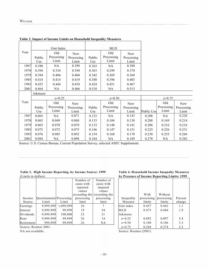
Public access to microdata requires the CensusBureau to limit some information to ensure the privacyand confidentiality of respondents. Topcoding income isone of the privacy measures used. For some years, thepublic-use topcodes and internal processing limits on theCPS ASEC were the same. Table 2 shows measures ofincome inequality derived from the CPS ASEC public-use data along with measures derived from internal Cen-sus Bureau data (Old/ New Processing Limits) for se-lected years. Public-use data show that, as with internaldata, all income inequality measures have increased overthe 1967-2001 period, but each of the public-use derived
- 6 -
WELNIAK
measures showed more growth than the internal mea-sures. The public-use Gini grew by 19 percent, com-pared to 17 percent using internal data; the MLD grewby 40 percent, compared to 36 percent; and the Atkinsongrew by between 34 percent and 45 percent, comparedto between 28 percent and 38 percent for internal data.8
The larger growth in income inequality using public-usedata is the result of: 1) topcoded income in 1967 whichreduced measured income inequality and 2) increasedhigh income through the plugging of mean topcoded val-ues beginning in 1996 (1997 CPS ASEC).
� Income Inequality Without Reporting Limits
In actuality, there are two restrictions that limit thereporting of high-income values on the CPS: a data col-lection limit and a processing limit. The questionnairelimits the reporting of income by restricting the numberof digits available for recording an amount during datacollection. This limit was set by physical restriction of apaper questionnaire. In 1993, this physical restrictionvirtually disappeared with the advent of computer-assisteddata collection. A data processing limit is applied to mini-mize the possible impact of recording (keying) errors,help maintain respondent confidentiality, and preventvolatility and distortion of annual statistics. It also com-promises the survey�s coverage of the income distributionand may understate income inequality. Prior to 1993, in-come recording and processing limits were the same.
Table 3 shows the current questionnaire and pro-cessing limits and the number of people who exceededthe processing limits for selected income sources on the2000 CPS. There were no cases that reported incomein excess of the data capture limit.
Allowing unrestricted income reporting increasedaggregate household income by about 0.1 percent andaffected income inequality measures to varying degrees.The Gini index was the measure least affected by al-lowing unrestricted income reporting, showing an increaseof 1.1 percent (see Table 4). The MLD was slightlymore affected, increasing 1.9 percent. Unrestricted in-come reporting had the most effect on the three Atkinsonmeasures. As would be expected, the measure with thehighest sensitivity to changes in the upper end of the
income distribution (e=0.25) increased 5.4 percent, whilethe measure most sensitive to changes in the lower endof the distribution (e=0.75) increased only 2.2 percent.
� High-Income Sample Turnover and Its Impacton Income Inequality Measures
One major concern with allowing the unrestrictedreporting for high-income cases is sample turnover andthe impact the loss or gain of very high-income samplecases could have on interpreting annual changes in in-come inequality. For example, an examination of highincome reporting on the 1999 CPS ASEC (1998 income)and the 2000 CPS ASEC (1999 income) showed thatsample turnover accounted for the loss of four high in-come households, with one of the those households hav-ing a maximum $9,999,999 in earnings reported. Be-tween 1998 and 1999, there was virtually no change inany of the income inequality measures.9
� Comparison of CPS Income Data WithAdministrative Sources
Any income inequality measure is only as good asthe data used to construct it. One way to gauge thequality of the CPS ASEC income is by comparing it toindependent sources. This section uses National Incomeand Product Account (NIPA) summaries and matchedInternal Revenue Service individual tax return informa-tion as benchmarks for evaluating CPS ASEC incomedata (see Roemer for a discussion of how to reconcilethe NIPA and CPS ASEC income definitions).
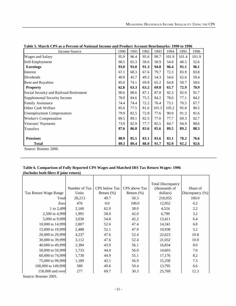
The most recent comparison of CPS and NIPA datauses 1996 income data. Table 5 shows that CPS aggre-gate income in 1996 was at 93 percent of NIPA bench-marks. The quality of CPS data varied widely from 53percent for self-employment income to 102 percent forwages and salaries. Since 1990, most of the income group-ings (earnings, property, and transfers) have shown a gen-eral trend toward slightly improved CPS data quality. Pen-sions, however, registered a 12-percentage point decline.
Earnings are a major component of income. In 2001,over $5.3 trillion (82 percent) of the total $6.4 trillioncollected in the CPS ASEC were from earnings; 77 per-
- 7 -
MEASURING HOUSEHOLD INCOME INEQUALITY USING THE CPS
cent were from wages and salaries alone. A recent studymatched 28,213 1996 IRS tax units to fully reported 1997CPS ASEC records. Table 6 shows how well the CPSASEC-reported wage data corresponded with tax databy tax wage interval. Approximately equal proportionsof CPS wage earners reported amounts above taxamounts as did earners reporting amounts below. Thetotal reporting discrepancy amounted to $210 million, or23 percent of the $913 million reported by these CPShouseholds. Roemer�s work with these matched data(2001) found that the CPS ASEC netted excess aggre-gate wages in all of the income intervals except the high-est, $150,000 and over.
� Conclusions
Each of the inequality measures examined using in-ternal CPS ASEC data painted a similar picture of chang-ing household income inequality over the 1967-2001 pe-riod. Overall, income inequality rose between 17 per-cent and 38 percent, depending on the measure.
The methodological changes that occurred in the 1971and the 1994 CPS ASECs had a noticeable impact oninequality measurement. With nearly one-third of thehouseholds on the 1971 CPS ASEC having restrictedincomes due to income reporting limits, income inequal-ity may have been understated by between 15 percentto 28 percent in prior years. A much smaller percentageof households (0.3 percent) were affected by the intro-duction of higher income recording limits in the 1994 CPSASEC, resulting in a possible understatement of incomeinequality of between 2 percent and 8 percent.
The CPS ASEC has been criticized for its inabilityto accurately measure income inequality because it failsto collect high-income values. A review of income in-equality measures using unrestricted income values reportedon the March 2000 CPS showed that processing limitsonly modestly affected estimates of income inequality.Removing the processing limits would increase measuredincome inequality by between 1 percent and 5 percent.
Restricted income information on the public-use ver-sion of the CPS ASEC causes a further reduction ofmeasured income inequality in years prior to 1996. The
plugging of mean values for topcoded respondents be-ginning with the 1997 public-use CPS ASEC broughtpublic measurement of income inequality more in linewith internal measurement. The net result, however, isan overstatement of income inequality growth over the1967-2001 period.
A review of independent benchmarks showed thatthe quality of the CPS ASEC income data seemed rea-sonable. Overall, aggregate CPS ASEC income was at93 percent of NIPA totals. A comparison to tax returnsshowed that the CPS ASEC had more reported wagesthan on tax returns in all but the highest income categories
� References
Technical Paper 17 (1967), �Trends in the Income ofFamilies and Persons in the United States: 1947-1964,� U.S. Government Printing Office, Wash-ington, DC.
Current Population Report, Series P60-204 (2000),�The changing Shape of the Nation�s IncomeDistribution: 1947-1998.� Government PrintingOffice, Washington, DC.
Jones, Arthur Jr, �Measuring Household IncomeInequality, 1967-1997,� presented at the JointStatistical Meetings for the American StatisticalAssociation, Baltimore, Maryland, August 1999.
Roemer, Marc (2000), �Assessing the Quality of theMarch Current Population Survey and the Surveyof Income and Program Participation IncomeEstimates 1990-1996,� U.S. Census Bureau.
Roemer, Marc, �An Evaluation of High IncomeReporting on the March Current PopulationSurvey (CPS),� U. S. Census Bureau, InternalMemorandum, March 2001.
Ryscavage, Paul, �A Surge in Growing IncomeInequality?,� Monthly Labor Review, August1995, pp. 51-61.
Welniak, Edward, �Effects of the March CurrentPopulation Survey�s New Processing System on
- 8 -
WELNIAK
Estimates of Income and Poverty,� 1990 ASA pro-ceedings.
� Footnotes
1 The CPS sample size increased in 2001 from ap-proximately 50,000 households to 78,000 to improveestimates for the State Children�s Health InsuranceProgram.
2 The ASEC was formerly known as the CPS MarchIncome Supplement.
3 People 14 years old and over prior to 1989.
4 The income limits were $9,999 for Social Security;$5,999 for Supplemental Security Income; $19,999for public assistance; and $29,999 for veterans�payments.
5 The growth rates in income inequality between 1967and 2001 for the MLD and Atkinson (e=.25 ande=.5) were not statistically different from one an-other.
6 The growth rates from 1967 to 1989 for the Giniand Atkinson (e=.25) were statistically differentfrom one another, as were the growth rates for theMLD and Atkinson (e=.25).
7 Between 1989 and 1991, the Atkinson Measurewith e=.25 declined 2.5 percent.
8 There was no difference between the MLD growthrate and the growth rates for the Atkinson e=0.25and e=0.5.
9 The MLD showed a significant decline of 2.7 per-cent.
- 9 -
MEASURING HOUSEHOLD INCOME INEQUALITY USING THE CPS
Table 1. Measures of Household Income Inequality: 1967 to 2001 Inequality Measures
Atkinson Year Gini Index MLD e=0.25 e=0.50 e=0.75
1967 0.399 0.380 0.071 0.143 0.220 1968 0.388 0.356 0.067 0.135 0.208 1969 0.391 0.357 0.067 0.135 0.209 1970 0.394 0.370 0.068 0.138 0.214 1971 0.396 0.370 0.068 0.138 0.214 1972 0.401 0.370 0.070 0.140 0.216 1973 0.397 0.355 0.068 0.136 0.210 1974 0.395 0.352 0.067 0.134 0.207 1975 0.397 0.361 0.067 0.136 0.210 1976 0.398 0.361 0.068 0.137 0.211 1977 0.402 0.364 0.069 0.139 0.213 1978 0.402 0.363 0.069 0.139 0.213 1979 0.404 0.369 0.070 0.141 0.216 1980 0.403 0.375 0.069 0.140 0.216 1981 0.406 0.387 0.070 0.141 0.220 1982 0.412 0.401 0.072 0.146 0.226 1983 0.414 0.397 0.072 0.147 0.226 1984 0.415 0.391 0.073 0.147 0.225 1985 0.419 0.403 0.075 0.151 0.231 1986 0.425 0.416 0.077 0.155 0.237 1987 0.426 0.414 0.077 0.155 0.238 1988 0.427 0.401 0.078 0.155 0.236 1989 0.431 0.406 0.080 0.158 0.239 1990 0.428 0.402 0.078 0.156 0.236 1991 0.428 0.411 0.078 0.156 0.237 1992 0.434 0.416 0.080 0.160 0.242 1993 0.454 0.467 0.092 0.178 0.266 1994 0.456 0.471 0.092 0.180 0.268 1995 0.450 0.452 0.090 0.175 0.261 1996 0.455 0.464 0.093 0.179 0.266 1997 0.459 0.484 0.094 0.183 0.272 1998 0.456 0.488 0.093 0.181 0.271 1999 0.457 0.475 0.092 0.180 0.268 2000 0.462 0.490 0.096 0.185 0.275 2001 0.466 0.515 0.098 0.189 0.282
Source: U.S. Census Bureau, Current Population Survey, selected ASEC Supplements.
- 10 -
WELNIAK
Table 2. Impact of Income Limits on Household Inequality Measures
Gini Index MLD Year
Public Use
Old Processing
Limit
New Processing
Limit Public Use
Old Processing
Limit
New Processing
Limit 1967 0.390 NA 0.399 0.363 NA 0.380 1970 0.394 0.334 0.394 0.363 0.299 0.370 1979 0.394 0.404 0.404 0.342 0.369 0.369 1985 0.414 0.414 0.419 0.380 0.396 0.403 1993 0.425 0.444 0.454 0.424 0.451 0.467 2001 0.464 NA 0.466 0.510 NA 0.515
Atkinson e=0.25 e=0.50 e=0.75
Year Public Use
Old Processing
Limit
New Processing
Limit Public Use
Old Processing
Limit
New Processing
Limit Public Use
Old Processing
Limit
New Processing
Limit 1967 0.065 NA 0.071 0.133 NA 0.143 0.208 NA 0.220 1970 0.065 0.049 0.068 0.133 0.104 0.138 0.208 0.169 0.214 1979 0.065 0.070 0.070 0.133 0.140 0.141 0.206 0.216 0.216 1985 0.072 0.072 0.075 0.146 0.147 0.151 0.225 0.226 0.231 1993 0.076 0.085 0.092 0.154 0.168 0.178 0.238 0.255 0.266 2001 0.094 NA 0.098 0.184 NA 0.189 0.278 NA 0.282
Source: U.S. Census Bureau, Current Population Survey, selected ASEC Supplements.
Table 3. High Income Reporting, by Income Source: 1999 Table 4. Household Income Inequalty Measures (Limits in dollars) by Presence of Income Reporting Limits: 1999
Income Source
Questionnaire Limit
Processing Limit
Number of cases with reported values
exceeding the processing
limit
Number of cases with imputed values
exceeding the processing
limit Inequality Measure
With processing
limits
Without processing
limits Percent change
Earnings 9,999,999 1,099,999 26 7 Gini index 0.457 0.462 1.1 Interest 9,999,999 99,999 19 54 MLD 0.475 0.484 1.9 Dividends 9,999,999 100,000 23 21 Atkinson: Rent 9,999,999 99,999 26 14 e=0.25 0.092 0.097 5.4 Retirement 999,999 99,999 26 NA e=0.50 0.180 0.186 3.3 Source: Roemer 2001. e=0.75 0.268 0.274 2.2 NA not available. Source: Roemer (2001)
- 11 -
MEASURING HOUSEHOLD INCOME INEQUALITY USING THE CPS
Table 5. March CPS as a Percent of National Income and Product Account Benchmarks: 1990 to 1996 Income Source 1990 1991 1992 1993 1994 1995 1996
Wages and Salary 95.9 96.4 95.6 99.7 101.9 101.4 101.9 Self-Employment 68.5 65.3 58.6 58.9 54.8 48.5 52.6 Earnings 93.0 93.0 91.3 94.8 96.4 95.1 96.1 Interest 67.1 68.3 67.6 79.7 72.3 83.9 83.8 Dividends 40.9 45.7 49.2 54.3 54.6 62.6 59.4 Rent and Royalties 85.0 74.1 69.8 65.2 64.8 58.7 58.6 Property 62.8 63.3 63.2 69.8 65.7 72.9 70.9 Social Security and Railroad Retirement 90.6 88.6 87.1 87.8 92.3 92.0 91.7 Supplemental Security Income 78.9 84.6 75.5 84.2 78.0 77.1 84.2 Family Assistance 74.4 74.4 72.2 76.4 73.1 70.5 67.7 Other Cash Welfare 85.6 77.5 81.6 101.3 105.2 95.8 80.5 Unemployment Compensation 79.9 82.5 72.8 77.6 90.0 91.3 81.6 Worker's Compensation 89.5 89.1 82.5 77.0 77.7 69.3 62.7 Veterans’ Payments 73.9 82.9 77.7 85.5 84.7 94.9 89.6 Transfers 87.6 86.8 83.6 85.6 89.5 89.2 88.3 Pensions 88.9 85.5 83.1 83.6 83.1 78.2 76.6 Total 89.3 89.4 88.0 91.7 92.9 92.2 92.6 Source: Roemer 2000.
Table 6. Comparison of Fully Reported CPS Wages and Matched IRS Tax Return Wages: 1996 (Includes both filers if joint return)
Tax Return Wage Range Number of Tax
Units CPS below Tax
Return (%) CPS above Tax
Return (%)
Total Discrepancy (thousands of
dollars) Share of
Discrepancy (%) Total 28,213 49.7 50.3 210,055 100.0 Zero 476 0.0 100.0 12,952 6.2
1 to 2,499 2,160 62.0 38.0 4,524 2.2 2,500 to 4,999 1,991 58.0 42.0 6,799 3.2 5,000 to 9,999 3,030 54.8 45.2 13,411 6.4
10,000 to 14,999 2,807 52.6 47.4 14,341 6.8 15,000 to 19,999 2,488 52.1 47.9 10,938 5.2 20,000 to 29,999 4,237 47.6 52.4 22,623 10.8 30,000 to 39,999 3,112 47.6 52.4 21,032 10.0 40,000 to 49,999 2,394 43.9 56.1 16,834 8.0 50,000 to 59,999 1,733 44.0 56.0 14,603 7.0 60,000 to 74,999 1,730 44.9 55.1 17,176 8.2 75,000 to 99,999 1,189 43.1 56.9 15,258 7.3
100,000 to 149,999 589 49.6 50.4 13,795 6.6 150,000 and over 277 69.7 30.3 25,769 12.3
Source: Roemer 2001.
- 13 -
An Analysis of the Distribution of Individual Incomeand Taxes, 1979-2001
Michael Strudler and Tom Petska, Internal Revenue Service,and Ryan Petska, Ernst and Young LLP
D ifferent approaches have been used to measurethe distribution of individual income over time.Survey data have been compiled with compre-
hensive enumeration, but underreporting of incomes, in-adequate coverage at the highest income levels, andomission of a key income type jeopardize the validity ofresults. Administrative records, such as income tax re-turns, may be less susceptible to underreporting of in-come but exclude certain nontaxable income types andcan be inconsistent in periods when the tax law has beenchanged. Record linkage studies have capitalized onthe advantages of both approaches, but are costly andseverely restricted by the laws governing interagencydata sharing.
This paper is the fifth in a series examining trends inthe distribution of individual incomes and tax burdensbased on a consistent and comprehensive measure ofincome derived from individual income tax returns.1,2,3,4
In the previous papers, we demonstrated that the sharesof income accounted for by the highest income-sizeclasses clearly have increased over time, and we alsodemonstrated the superiority of our comprehensive andconsistent income measure, the 1979 Retrospective In-come Concept, particularly in periods of tax reform. Inthis paper, we continue the analysis of individual incomeand tax distributions, adding for 3 years (1979, 1989, and1999) Social Security and Medicare taxes to this analy-sis. The paper has three sections. In the first section,we briefly summarize this measure of individual incomederived as a “retrospective concept” from individual in-come tax returns. In the second section, we present theresults of our analysis of time series data. We concludewith an examination of Gini coefficients computed fromthese data.
� Derivation of the Retrospective IncomeConcept
The tax laws of the 1980’s and 1990’s made signifi-cant changes to both the tax rates and definitions of tax-able income. The tax reforms of 1981 and 1986 signifi-
cantly lowered individual income tax rates, and the latteralso substantially broadened the income tax base. Thetax law changes effective for 1991 and 1993 initiatedrising individual income tax rates and further modifica-tions to the definition of taxable income.1,2,3,4 Lawchanges effective for 1997 substantially lowered themaximum tax rate on capital gains. The newest lawchanges have lowered marginal rates starting with 2001and will again lower the maximum tax rate on long-termcapital gains, as well as decrease the maximum ratesfor most dividends. With all of these changes, the ques-tions that arise are what has happened to the distributionof individual income, the shares of taxes paid, and aver-age taxes by the various income-size classes?
In order to analyze changes in income and taxesover time, consistent definitions of income and taxes mustbe used. However, the Internal Revenue Code has beensubstantially changed in the last 23 years—both the con-cept of taxable income and the tax rate schedules havebeen significantly altered. The most commonly used in-come concept available from Federal income tax returns,Adjusted Gross Income (AGI), has changed over timemaking it difficult to use AGI for inter-temporal com-parisons of income. For this reason, an income defini-tion that would be both comprehensive and consistentover time was developed.5, 6, 7, 8 The 1979 RetrospectiveIncome Concept was designed to include the same in-come and deduction items from items available on Fed-eral individual income tax returns. Tax Years 1979 through1986 were used as base years to identify the incomeand deduction items, and the concept was subsequentlyapplied to later years, including the same componentscommon to all years.
The calculation of the 1979 Retrospective IncomeConcept includes several items partially excluded fromAGI for the base years, the largest of which was capitalgains. 1,2,3,4 The full amounts of all capital gains, as wellas all dividends and unemployment compensation, wereincluded in the income calculation. Total pensions, annu-ities, IRA distributions, and rollovers were added, includ-

- 14 -
STRUDLER, PETSKA, AND PETSKA
ing nontaxable portions that were excluded from AGI.Social Security benefits were omitted because they werenot reported on tax returns until 1984. Also, any depre-ciation in excess of straight-line depreciation, which wassubtracted in computing AGI, was added back. For thisstudy, retrospective income was computed for all indi-vidual income tax returns in the annual Statistics of In-come (SOI) sample files for the period 1979 through2001. Loss returns were excluded, and the tax returnswere tabulated into income-size classes based on thesize of retrospective income and ranked from highest tolowest. Percentile thresholds were estimated or inter-polated for income-size classes ranging from the top 0.1percent to the bottom 20 percent.9,10,11 For each sizeclass, the number of returns and the amounts of retro-spective income and taxes paid were compiled. Fromthese data, income and tax shares and average taxeswere computed for each size class for all years.
� The Distribution of Income and Taxes
With this data base, we sought to answer the fol-lowing questions—have the distribution of individual in-comes (i.e., income shares), the distribution of taxes (i.e.,tax shares), and the average effective tax rates (i.e.,
tax burdens) changed over time? As a first look at thedata, we examined the income thresholds of the bottom(or entry level) of each income-size class, and a clearpattern emerged. While all of the income thresholds haveincreased over time, the largest increases in absoluteterms, and on a percentage basis, were with the highestincome-size classes.
For example, while $233,539 were needed to enterthe top 0.1 percent for 1979, $1,405,770 were neededfor entry into this class for 2001. This represents a morethan 500-percent increase. Also, while $79,679 of ret-rospective income were needed to enter the top 1-per-cent size class for 1979, $323,861 were needed for en-try into this size class for 2001, an increase of 306 per-cent. For the top 20 percent, the threshold increased by159 percent, and, for the bottom 20 percent, the increasewas only 124 percent. Since much of these increasesare attributable to inflation, we computed constant dollarthresholds, using the Consumer Price Index.12
What is most striking about these data are thechanges between 1979 and 2001 for the various income-size percentile thresholds (see Figure A). For example,the threshold for the top 0.1 percent grew (using a 1982-
Figure A. Constant Dollar Income Thresholds, 1979-2001 (1982-84=100)
0
200000
400000
600000
800000
1000000
1200000
1979 1980 1981 1982 1983 1984 1985 1986 1987 1988 1989 1990 1991 1992 1993 1994 1995 1996 1997 1998 1999 2000 2001Years
Who
le D
olla
rs
Top .1% Top 1% Top 5% Top 10% Top 20%
- 15 -
AN ANALYSIS OF THE DISTRIBUTION OF INDIVIDUAL INCOME AND TAXES, 1979-2001
1984 base) from $321,679 for 1979 to $793,772 for 2001,an increase of 147 percent. Similarly, the threshold forthe taxpayers in the 1-percent group rose from $109,751for 1979 to $182,869 for 2001, an increase of over 66percent. However, the thresholds for each lower per-centile class show smaller increases in the period; thetop 20-percentile threshold increased only 6.1 percent,and the 40-percent and all lower thresholds all declined.
Income Shares
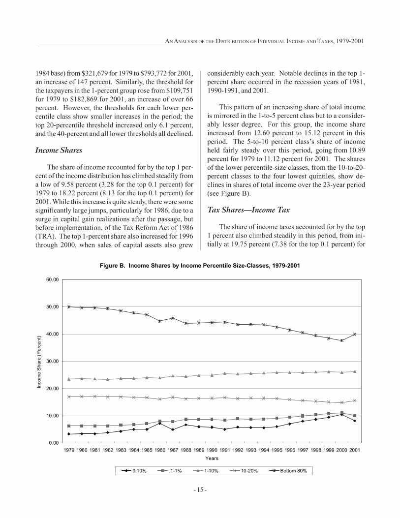
The share of income accounted for by the top 1 per-cent of the income distribution has climbed steadily froma low of 9.58 percent (3.28 for the top 0.1 percent) for1979 to 18.22 percent (8.13 for the top 0.1 percent) for2001. While this increase is quite steady, there were somesignificantly large jumps, particularly for 1986, due to asurge in capital gain realizations after the passage, butbefore implementation, of the Tax Reform Act of 1986(TRA). The top 1-percent share also increased for 1996through 2000, when sales of capital assets also grew
considerably each year. Notable declines in the top 1-percent share occurred in the recession years of 1981,1990-1991, and 2001.
This pattern of an increasing share of total incomeis mirrored in the 1-to-5 percent class but to a consider-ably lesser degree. For this group, the income shareincreased from 12.60 percent to 15.12 percent in thisperiod. The 5-to-10 percent class’s share of incomeheld fairly steady over this period, going from 10.89percent for 1979 to 11.12 percent for 2001. The sharesof the lower percentile-size classes, from the 10-to-20-percent classes to the four lowest quintiles, show de-clines in shares of total income over the 23-year period(see Figure B).
Tax Shares—Income Tax
The share of income taxes accounted for by the top1 percent also climbed steadily in this period, from ini-tially at 19.75 percent (7.38 for the top 0.1 percent) for
Figure B. Income Shares by Income Percentile Size-Classes, 1979-2001
0.00
10.00
20.00
30.00
40.00
50.00
60.00
1979 1980 1981 1982 1983 1984 1985 1986 1987 1988 1989 1990 1991 1992 1993 1994 1995 1996 1997 1998 1999 2000 2001Years
Inco
me
Shar
e (P
erce
nt)
0.10% .1-1% 1-10% 10-20% Bottom 80%
- 16 -
STRUDLER, PETSKA, AND PETSKA
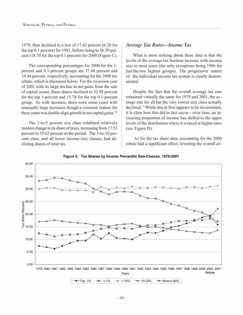
1979, then declined to a low of 17.42 percent (6.28 forthe top 0.1 percent) for 1981, before rising to 36.30 per-cent (18.70 for the top 0.1 percent) for 2000 (Figure C).
The corresponding percentages for 2000 for the 1-percent and 0.1-percent groups are 37.68 percent and19.44 percent, respectively, accounting for the 2000 taxrebate, which is discussed below. For the recession yearof 2001 with its large decline in net gains from the saleof capital assets, these shares declined to 32.88 percentfor the top 1-percent and 15.78 for the top 0.1-percentgroup. As with incomes, there were some years withunusually large increases though a common feature forthese years was double-digit growth in net capital gains.7,8
The 1-to-5 percent size class exhibited relativelymodest change in its share of taxes, increasing from 17.53percent to 19.62 percent in the period. The 5-to-10 per-cent class, and all lower income-size classes, had de-clining shares of total tax.
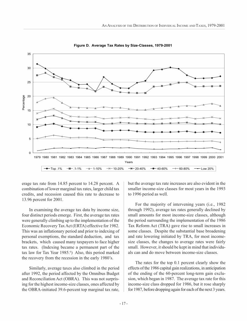
Average Tax Rates—Income Tax
What is most striking about these data is that thelevels of the average tax burdens increase with incomesize in most years (the only exceptions being 1986 forjust the two highest groups). The progressive natureof the individual income tax system is clearly demon-strated.
Despite the fact that the overall average tax rateremained virtually the same for 1979 and 2001, the av-erage rate for all but the very lowest size class actuallydeclined.13 While this at first appears to be inconsistent,it is clear how this did in fact occur—over time, an in-creasing proportion of income has shifted to the upperlevels of the distribution where it is taxed at higher rates(see Figure D).
As for the tax share data, accounting for the 2000rebate had a significant effect, lowering the overall av-
Figure C. Tax Shares by Income Percentile Size-Classes, 1979-2001
0.00
5.00
10.00
15.00
20.00
25.00
30.00
35.00
40.00
1979 1980 1981 1982 1983 1984 1985 1986 1987 1988 1989 1990 1991 1992 1993 1994 1995 1996 1997 1998 1999 2000 2000Rebate
2001Years
Tax
Shar
e (P
erce
nt)
Top .1% .1-1% 1-10% 10-20% Bottom 80%
- 17 -
AN ANALYSIS OF THE DISTRIBUTION OF INDIVIDUAL INCOME AND TAXES, 1979-2001
erage tax rate from 14.85 percent to 14.28 percent. Acombination of lower marginal tax rates, larger child taxcredits, and recession caused this rate to decrease to13.96 percent for 2001.
In examining the average tax data by income size,four distinct periods emerge. First, the average tax rateswere generally climbing up to the implementation of theEconomic Recovery Tax Act (ERTA) effective for 1982.This was an inflationary period and prior to indexing ofpersonal exemptions, the standard deduction, and taxbrackets, which caused many taxpayers to face highertax rates. (Indexing became a permanent part of thetax law for Tax Year 1985.6) Also, this period markedthe recovery from the recession in the early 1980’s.
Similarly, average taxes also climbed in the periodafter 1992, the period affected by the Omnibus Budgetand Reconciliation Act (OBRA). This was not surpris-ing for the highest income-size classes, ones affected bythe OBRA-initiated 39.6-percent top marginal tax rate,
but the average tax rate increases are also evident in thesmaller income-size classes for most years in the 1993to 1996 period as well.
For the majority of intervening years (i.e., 1982through 1992), average tax rates generally declined bysmall amounts for most income-size classes, althoughthe period surrounding the implementation of the 1986Tax Reform Act (TRA) gave rise to small increases insome classes. Despite the substantial base broadeningand rate lowering initiated by TRA, for most income-size classes, the changes to average rates were fairlysmall. However, it should be kept in mind that individu-als can and do move between income-size classes.
The rates for the top 0.1 percent clearly show theeffects of the 1986 capital gain realizations, in anticipationof the ending of the 60-percent long-term gain exclu-sion, which began in 1987. The average tax rate for thisincome-size class dropped for 1986, but it rose sharplyfor 1987, before dropping again for each of the next 3 years.
Figure D. Average Tax Rates by Size-Classes, 1979-2001
0
5
10
15
20
25
30
35
1979 1980 1981 1982 1983 1984 1985 1986 1987 1988 1989 1990 1991 1992 1993 1994 1995 1996 1997 1998 1999 2000 2001Years
Perc
enta
ge
Top .1% .1-1% 1-10% 10-20% 20-40% 40-60% 60-80% Low 20%
- 18 -
STRUDLER, PETSKA, AND PETSKA
To assess what happened, it is important to look atthe underlying data. The substantial increase in capitalgain realizations for 1986 swelled the aggregate incomeand tax amounts for upper income classes and also raisedthe income thresholds of these top classes. However,since much of the increase in income for these sizeclasses was from net long-term capital gains, which hada maximum effective tax rate of 20 percent, it is notsurprising that the average tax rate for these top sizeclasses declined.
Last, are those years affected by the Taxpayer Re-lief Act of 1997 (1997 through 2001), where the top rateon long-term capital gains was reduced significantly from28 percent to 20 percent. For 1997, the first year underthis law, when the lower rates were only partially in ef-fect, the average tax rate fell for the top 0.1-percentgroup of taxpayers but increased for all other groups.However, for 1998, the first full year under lower capitalgain rates, all groups up to and including the 40-to-60percent class had reduced average tax rates (while thelowest two quintiles had virtually the same average taxrates). For all groups (except for the 20-40 and the 60-to-80 percent groups in 1999), the average rates returnedto increasing for both 1999 and 2000.
The Economic Growth and Tax Relief Reconcilia-tion Act of 2001 (EGTRRA) further reduced marginaltax rates over several years. One of these reductionswas an introduction of a 10-percent bracket on the first$6,000 ($12,000 if married filing a joint return) of taxableincome. In an attempt to fuel a recovery from reces-sion, this reduction was introduced retroactively in theform of a rebate based on Tax Year 2000 filings. There-fore, we simulated the rebate on the Tax Year 2000 Indi-vidual File to see its effects on average tax rates. Whenthe rebate is taken into account, the average rates for2000 decreased for all groups, except for the top 0.1 and
the 1-to-5 percent, reversing the pre-rebate increases.Tax Year 2001 was a mixture of increases and decreasesin average tax rates by income group. Most groups paidhigher average taxes; however, the 1-to-5 and 5-to-10percent groups paid lower average taxes along with thebottom 20-percent group.
Tax Shares—Income Plus Social Security Tax
For individual taxpayers, Social Security taxes com-pose a fairly large portion (about 37 percent for 1999) ofthe Federal tax burden.14 To broaden our analysis,we merged data from W-2’s with individual income taxrecords for the years 1979, 1989, and 1999. Total socialsecurity taxes included self-employment taxes and taxeson tips reported on tax returns and two times the socialsecurity taxes (representing both the taxpayers’ and theemployers’ shares) reported on
W-2’s. The employers’ share of this tax was addedinto retrospective income, as well. To further help ouranalysis, the U.S. Treasury Department’s Office of TaxAnalysis (OTA) model was used to simulate the effectof the two new tax laws (EGTRRA) and the Jobs andGrowth Tax Relief Reconciliation Act of 2003(JGTRRA), on the 1999 data.15
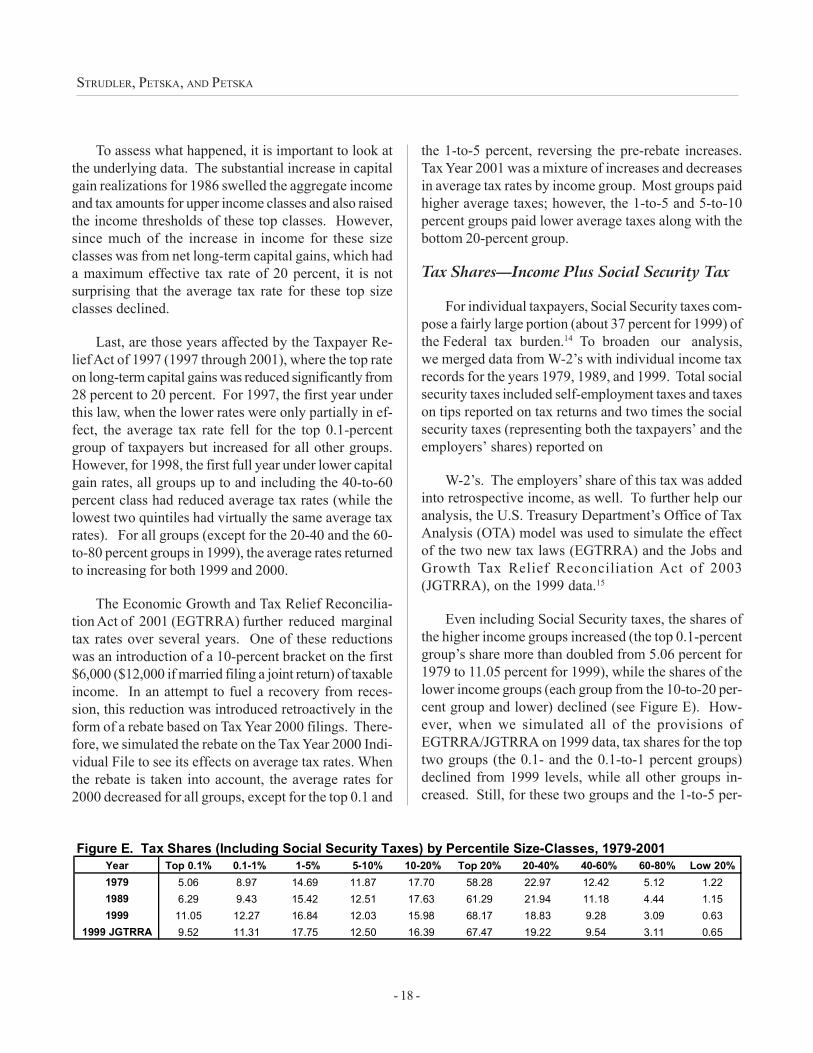
Even including Social Security taxes, the shares ofthe higher income groups increased (the top 0.1-percentgroup’s share more than doubled from 5.06 percent for1979 to 11.05 percent for 1999), while the shares of thelower income groups (each group from the 10-to-20 per-cent group and lower) declined (see Figure E). How-ever, when we simulated all of the provisions ofEGTRRA/JGTRRA on 1999 data, tax shares for the toptwo groups (the 0.1- and the 0.1-to-1 percent groups)declined from 1999 levels, while all other groups in-creased. Still, for these two groups and the 1-to-5 per-
Figure E. Tax Shares (Including Social Security Taxes) by Percentile Size-Classes, 1979-2001 Year Top 0.1% 0.1-1% 1-5% 5-10% 10-20% Top 20% 20-40% 40-60% 60-80% Low 20%
1979 5.06 8.97 14.69 11.87 17.70 58.28 22.97 12.42 5.12 1.221989 6.29 9.43 15.42 12.51 17.63 61.29 21.94 11.18 4.44 1.151999 11.05 12.27 16.84 12.03 15.98 68.17 18.83 9.28 3.09 0.63
1999 JGTRRA 9.52 11.31 17.75 12.50 16.39 67.47 19.22 9.54 3.11 0.65
- 19 -
AN ANALYSIS OF THE DISTRIBUTION OF INDIVIDUAL INCOME AND TAXES, 1979-2001
cent, the tax shares were still higher than 1989 levels.Interestingly, the 1-to-5 percent group is the only groupwhose share increased from 1989 to 1999 (from 15.42percent to 16.84 percent) and then increased again (to17.85 percent) under new tax law provisions. This ismost likely due to the effect of the alternative minimumtax (AMT) offsetting lower marginal and capital gainrates for this group of taxpayers.
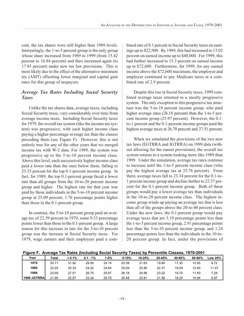
Average Tax Rates Including Social SecurityTaxes
Unlike the tax shares data, average taxes, includingSocial Security taxes, vary considerably over time fromaverage income taxes. Including Social Security taxesfor 1979, the overall tax system (like the income tax sys-tem) was progressive, with each higher income classpaying a higher percentage average tax than the classespreceding them (see Figure F). However, this is notentirely true for any of the other years that we mergedincome tax with W-2 data. For 1989, the system wasprogressive up to the 5-to-10 percent income class.Above this level, each successively higher income classpaid a lower rate than the ones below them, falling to23.33 percent for the top 0.1-percent income group. Infact, for 1989, the top 0.1-percent group faced a lowerrate than all groups from the 10-to-20 percent incomegroup and higher. The highest rate for that year waspaid by those individuals in the 5-to-10 percent incomegroup at 25.09 percent, 1.76 percentage points higherthan those in the 0.1-percent group.
In contrast, the 5-to-10 percent group paid an aver-age tax of 22.59 percent in 1979, some 9.33 percentagepoints lower than those in the 0.1-percent group. A largereason for this increase in rate for the 5-to-10 percentgroup was the increase in Social Security taxes. For1979, wage earners and their employers paid a com-
bined rate of 8.1 percent in Social Security taxes on earn-ings up to $22,900. By 1989, this had increased to 13.02percent on earned income up to $48,000. For 1999, thishad further increased to 15.3 percent on earned incomeup to $72,600. Furthermore, for 1999, for any earnedincome above the $72,600 maximum, the employee andemployer continued to pay Medicare taxes at a com-bined rate of 2.9 percent.
Despite this rise in Social Security taxes, 1999 com-bined average taxes returned to a mostly progressivesystem. The only exception to this progressive tax struc-ture was the 5-to-10 percent income group, who paidhigher average rates (26.18 percent) than the 1-to-5 per-cent income group (25.97 percent). However, the 0.1-to-1 percent and the 0.1-percent income groups paid thehighest average taxes at 26.70 percent and 27.51 percent.
When we simulated the provisions of the two newtax laws (EGTRRA and JGTRRA) on 1999 data (with-out allowing for the sunset provisions), the overall taxsystem returns to a system looking more like 1989 than1999. Under the simulation, average tax rates continueto increase until the 1-to-5 percent income class (whopay the highest average tax at 25.76 percent). Fromthere, average taxes fall to 23.34 percent for the 0.1-to-1 percent income group and decline further to 22.57 per-cent for the 0.1-percent income group. Both of thesegroups would pay a lower average tax than individualsin the 10-to-20 percent income class. The highest in-come group winds up paying an average tax that is lessthan all of the groups above the 20-to-40 percent class.Under the new laws, the 0.1-percent group would payaverage taxes that are 3.19 percentage points less thanthe 1-to-5 percent income group, 2.91 percentage pointsless than the 5-to-10 percent income group, and 1.24percentage points less than the individuals in the 10-to-20 percent group. In fact, under the provisions of
Figure F. Average Tax Rates (Including Social Security Taxes) by Percentile Classes, 1979-2001 Year Total < 0.1% 0.1 - 1% 1-5% 5-10% 10-20% 20-40% 40-60% 60-80% Low 20%
1979 20.71 31.92 29.50 24.14 22.59 21.63 19.89 17.35 12.65 8.721989 22.24 23.33 24.22 24.84 25.09 23.90 22.37 19.29 13.93 11.471999 23.59 27.51 26.70 25.97 26.18 24.96 23.22 19.70 11.83 7.29
1999 JGTRRA 21.90 22.57 23.34 25.76 25.48 23.81 21.58 18.25 10.94 6.97
- 20 -
STRUDLER, PETSKA, AND PETSKA
EGTRRA/JGTRRA, the individuals in the 0.1-percentgroup wind up paying less than one percentage point(0.99) more than the 20-to-40 percent income group. Incontrast, the highest income group paid average combinedtaxes of 12.03 percentage points higher than the 20-to-40 percent income group in 1979 and 4.29 percentagepoints higher than this group under existing 1999 laws.
� Analysis of Gini Coefficients
To further analyze the data, we estimated Lorenzcurves and computed Gini coefficients for all years. TheLorenz curve is a cumulative aggregation of income fromlowest to highest, expressed on a percentage basis. Toconstruct the Lorenz curves, we reordered the percen-tile classes from lowest to highest and used the incomethresholds as “plotting points” to fit a series of regres-sion equations for each income-size interval in the 23years, both before- and after-taxes.
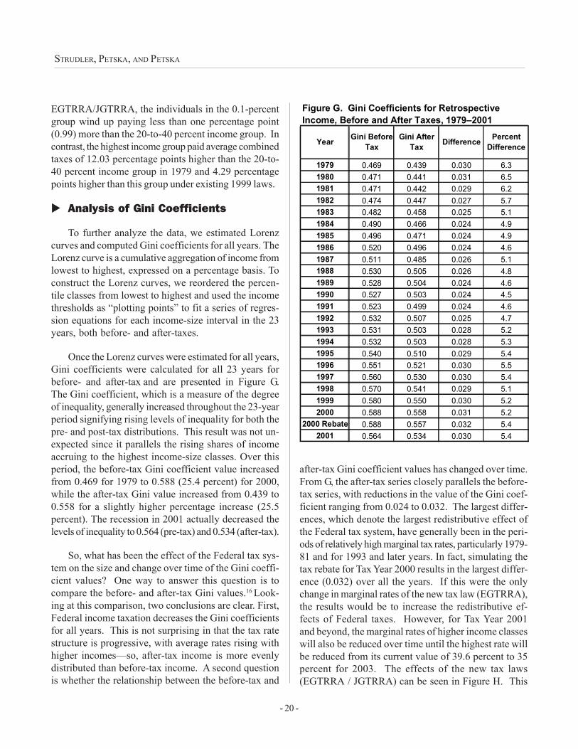
Once the Lorenz curves were estimated for all years,Gini coefficients were calculated for all 23 years forbefore- and after-tax and are presented in Figure G.The Gini coefficient, which is a measure of the degreeof inequality, generally increased throughout the 23-yearperiod signifying rising levels of inequality for both thepre- and post-tax distributions. This result was not un-expected since it parallels the rising shares of incomeaccruing to the highest income-size classes. Over thisperiod, the before-tax Gini coefficient value increasedfrom 0.469 for 1979 to 0.588 (25.4 percent) for 2000,while the after-tax Gini value increased from 0.439 to0.558 for a slightly higher percentage increase (25.5percent). The recession in 2001 actually decreased thelevels of inequality to 0.564 (pre-tax) and 0.534 (after-tax).
So, what has been the effect of the Federal tax sys-tem on the size and change over time of the Gini coeffi-cient values? One way to answer this question is tocompare the before- and after-tax Gini values.16 Look-ing at this comparison, two conclusions are clear. First,Federal income taxation decreases the Gini coefficientsfor all years. This is not surprising in that the tax ratestructure is progressive, with average rates rising withhigher incomes—so, after-tax income is more evenlydistributed than before-tax income. A second questionis whether the relationship between the before-tax and
after-tax Gini coefficient values has changed over time.From G, the after-tax series closely parallels the before-tax series, with reductions in the value of the Gini coef-ficient ranging from 0.024 to 0.032. The largest differ-ences, which denote the largest redistributive effect ofthe Federal tax system, have generally been in the peri-ods of relatively high marginal tax rates, particularly 1979-81 and for 1993 and later years. In fact, simulating thetax rebate for Tax Year 2000 results in the largest differ-ence (0.032) over all the years. If this were the onlychange in marginal rates of the new tax law (EGTRRA),the results would be to increase the redistributive ef-fects of Federal taxes. However, for Tax Year 2001and beyond, the marginal rates of higher income classeswill also be reduced over time until the highest rate willbe reduced from its current value of 39.6 percent to 35percent for 2003. The effects of the new tax laws(EGTRRA / JGTRRA) can be seen in Figure H. This
1979 0.469 0.439 0.030 6.31980 0.471 0.441 0.031 6.51981 0.471 0.442 0.029 6.21982 0.474 0.447 0.027 5.71983 0.482 0.458 0.025 5.11984 0.490 0.466 0.024 4.91985 0.496 0.471 0.024 4.91986 0.520 0.496 0.024 4.61987 0.511 0.485 0.026 5.11988 0.530 0.505 0.026 4.81989 0.528 0.504 0.024 4.61990 0.527 0.503 0.024 4.51991 0.523 0.499 0.024 4.61992 0.532 0.507 0.025 4.71993 0.531 0.503 0.028 5.21994 0.532 0.503 0.028 5.31995 0.540 0.510 0.029 5.41996 0.551 0.521 0.030 5.51997 0.560 0.530 0.030 5.41998 0.570 0.541 0.029 5.11999 0.580 0.550 0.030 5.22000 0.588 0.558 0.031 5.2
2000 Rebate 0.588 0.557 0.032 5.42001 0.564 0.534 0.030 5.4
Figure G. Gini Coefficients for Retrospective Income, Before and After Taxes, 1979–2001
Year Gini Before Tax
Gini After Tax Difference Percent
Difference
- 21 -
AN ANALYSIS OF THE DISTRIBUTION OF INDIVIDUAL INCOME AND TAXES, 1979-2001
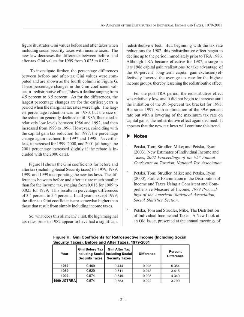
figure illustrates Gini values before and after taxes whenincluding social security taxes with income taxes. Thenew law decreases the difference between before- andafter-tax Gini values for 1999 from 0.025 to 0.022.
To investigate further, the percentage differencesbetween before- and after-tax Gini values were com-puted and are shown as the fourth column in Figure G.These percentage changes in the Gini coefficient val-ues, a “redistributive effect,” show a decline ranging from4.5 percent to 6.5 percent. As for the differences, thelargest percentage changes are for the earliest years, aperiod when the marginal tax rates were high. The larg-est percentage reduction was for 1980, but the size ofthe reduction generally declined until 1986, fluctuated atrelatively low levels between 1986 and 1992, and thenincreased from 1993 to 1996. However, coinciding withthe capital gain tax reduction for 1997, the percentagechange again declined for 1997 and 1998. Neverthe-less, it increased for 1999, 2000, and 2001 (although the2001 percentage increased slightly if the rebate is in-cluded with the 2000 data).
Figure H shows the Gini coefficients for before andafter tax (including Social Security taxes) for 1979, 1989,1999, and 1999 incorporating the new tax laws. The dif-ferences between before and after tax are much smallerthan for the income tax, ranging from 0.018 for 1989 to0.025 for 1979. This results in percentage differencesof 3.4 percent to 5.4 percent. In all years, except 1999,the after-tax Gini coefficients are somewhat higher thanthose that result from simply including income taxes.
So, what does this all mean? First, the high marginaltax rates prior to 1982 appear to have had a significant
redistributive effect. But, beginning with the tax ratereductions for 1982, this redistributive effect began todecline up to the period immediately prior to TRA 1986.Although TRA became effective for 1987, a surge inlate 1986 capital gain realizations (to take advantage ofthe 60-percent long-term capital gain exclusion) ef-fectively lowered the average tax rate for the highestincome groups, thereby lessening the redistributive effect.
For the post-TRA period, the redistributive effectwas relatively low, and it did not begin to increase untilthe initiation of the 39.6-percent tax bracket for 1993.But since 1997, with continuation of the 39.6-percentrate but with a lowering of the maximum tax rate oncapital gains, the redistributive effect again declined. Itappears that the new tax laws will continue this trend.
� Notes
1 Petska, Tom; Strudler, Mike; and Petska, Ryan(2003), New Estimates of Individual Income andTaxes, 2002 Proceedings of the 95th AnnualConference on Taxation, National Tax Association.
2 Petska, Tom; Strudler, Mike; and Petska, Ryan(2000), Further Examination of the Distribution ofIncome and Taxes Using a Consistent and Com-prehensive Measure of Income, 1999 Proceed-ings of the American Statistical Association,Social Statistics Section.
3 Petska, Tom and Strudler, Mike, The Distributionof Individual Income and Taxes: A New Look atan Old Issue, presented at the annual meetings of
1979 0.469 0.444 0.025 5.3541989 0.529 0.511 0.018 3.4151999 0.574 0.549 0.025 4.340
1999 JGTRRA 0.574 0.553 0.022 3.790
Figure H. Gini Coefficients for Retrospective Income (Including Social Security Taxes), Before and After Taxes, 1979-2001
Gini Before Tax Including Social Security Taxes
YearGini After Tax
Including Social Security Taxes
Difference Percent Difference
- 22 -
STRUDLER, PETSKA, AND PETSKA
the American Economic Association, New York,NY, January 1999, and published in TurningAdministrative Systems Into Information Sys-tems: 1998-1999.
4 Petska, Tom and Strudler, Mike (1999), Income,Taxes, and Tax Progressivity: An Examination ofRecent Trends in the Distribution of IndividualIncome and Taxes, 1998 Proceedings of theAmerican Statistical Association, Social Statis-tics Section.
5 Nelson, Susan (1987), Family Economic Incomeand Other Income Concepts Used in AnalyzingTax Reform, Compendium of Tax Research,1986, Office of Tax Analysis, U.S. Department ofthe Treasury.
6 Hostetter, Susan (1988), Measuring Income forDeveloping and Reviewing Individual Tax LawChanges: Exploration of Alternative Concepts,1987 Proceedings of the American StatisticalAssociation, Survey Research Methods Section.
7 Internal Revenue Service, Statistics of Income—Individual Income Tax Returns, Publication 1304,(selected years).
8 Parisi, Michael and Campbell, Dave, IndividualIncome Tax Rates and Tax Shares, 1999, Statis-tics of Income (SOI) Bulletin, Winter 2001-2002,Volume 21, Number 3.
9 For the years 1979 through 1992, the percentilethreshold size classes were estimated byosculatory interpolation as described in Oh and Ohand Scheuren.10, 11 In this procedure, the datawere tabulated into size classes, and the percentilethresholds were interpolated. For 1993 through2000, the SOI individual tax return data files weresorted from highest to lowest, and the percentilethresholds were determined by cumulating recordsfrom the top down.
1 0 Oh, H. Lock (1978), Osculatory Interpolations
with a Monotonicity Constraint, 1977 Proceed-ings of the American Statistical Association,Statistical Computing Section.
1 1 Oh, H. Lock and Scheuren, Fritz (1988),Osculatory Interpolations Revisited, 1987 Pro-ceedings of the American Statistical Associa-tion, Statistical Computing Section.
1 2 The CPI-U from the U.S. Department of Labor,Monthly Labor Review, was used for deflation ofthe income thresholds.
1 3 Taxes, taxes paid, tax liabilities, tax shares, andaverage or effective tax rates are based onincome tax, defined as income tax after creditsplus alternative minimum tax (AMT) less thenonrefundable portion of the earned income credit(for 2000 and 2001, AMT was included in incometax after credits). However, for Figure F, taxincludes Social Security and Medicare taxes lessall of the earned income credit and refundablechild credit.
1 4 Internal Revenue Service, Data Book 1999,Publication 55B. Total Individual Income Taxescollected from withholding and additional taxespaid with tax forms filed were $1,102.2 billion,while total Social Security taxes were $587.5 billion.
1 5 Actually, the OTA model was computed on 1998individual income tax data and programmed totake all aspects of JGTRRA into account underthe assumption that all of the sunset provisions willremain in place. After the results were calculated,the data were increased to 1999 levels. There-fore, income is exactly the same as the rest of the1999 data, and only the taxes paid differs.
1 6 A comparison of the before- and after-tax Ginicoefficients does not exclusively measure theeffects of the tax system in that the tax laws canalso affect before-tax income. For example,capital gain realizations have been shown to besensitive to the tax rates.
- 23 -
The Distribution of Household Income:Two Decades of Change¹
Roberton Williams, Congressional Budget Office
A verage household income grew by more than 40percent in real terms between 1979 and 2000,climbing from $52,300 to $74,200 (in 2000 dol-
lars). The rate of income growth varied sharply acrossthe income distribution, however. Average real incomeof the lowest quintile�or fifth of the distribution�in-creased just 7 percent over the 21-year period, com-pared with a 70-percent gain for the top quintile. Growthwas even faster at the very top of the distribution: realincome for the top 5 percent of households more thandoubled, and that of the top 1 percent nearly tripled.Income growth also varied across types of households:incomes of households with children increased at aboutthe same rate as those of all households, incomes ofnonelderly childless households grew more slowly, andincomes of the elderly climbed nearly half again as fastas the overall average.
This paper examines trends in household incomebetween 1979 and 2000, utilizing a measure that includesboth cash and in-kind income. To look at changes in thedistribution of income, the paper divides households intoquintiles and further subdivides the top quintile into fourparts�the 80th-90th percentiles, the 90th-95th percen-tiles, the 95th-99th percentiles, and the top 1 percent.2
Analysis includes both pretax and post-tax income toassess the effects of taxes on the distribution of income.The paper also separates households into three typesbased on the presence of children and the age of thehousehold head. The paper is purely descriptive; it makesno attempt to examine why incomes changed as theydid or to analyze patterns of change among componentsof income.
� Measuring Income
The principal income measure used in this paper ispretax comprehensive household income. That mea-sure counts both cash and in-kind income, including:
� all cash income (both taxable and tax-exempt);
� taxes paid by businesses (the employer shareof payroll taxes is imputed to workers, and cor-porate income taxes are imputed to owners ofcapital);
� employee contributions to 401(k) retirementplans; and
� the value of income received in kind from vari-ous sources (including employer-paid healthinsurance premiums, Medicare, Medicaid, foodstamps, housing and energy assistance, andschool breakfasts and lunches).
Income thus includes more sources than people of-ten consider in assessing their well-being. Furthermore,income is counted when it is reported, generally for taxpurposes. Thus, capital gains are included in incomewhen they are realized, even though they may have ac-crued over many years and might thus be more appro-priately counted on an accrual basis (that is, the increaseor decrease in value in a given year would count as in-come in that year).3 As a result, households that realizelarge gains in a given year may show higher up the in-come distribution than they would in an average year,and the distribution based on that measure of incomewould appear to be more unequal than if based on anaccrued income measure.
A second measure�after-tax comprehensive house-hold income�is comparable to the pretax measure de-scribed above but subtracts the major Federal taxes paidby the household: individual and corporate income taxes,payroll taxes, and excise taxes.4 Comparing the twomeasures thus shows the impact of major Federal taxeson the distribution of income.
The unit of observation is the household�groups ofpeople sharing the same living quarters, regardless oftheir relationships. Households thus include single peopleliving by themselves, nuclear families with no nonfamily
- 24 -
WILLIAMS
members living with them, unmarried couples living to-gether, and groups of unrelated people sharing a houseor apartment, among many other possibilities. In mostcases, members of households share all costs out of theircommon income, and the household is the appropriateunit over which to measure income. In some cases, theonly sharing of income is for housing costs, and house-hold members cover their own expenses for everythingelse; for those groups, using household as the unit ofmeasurement misstates members� well-being.5
Placement of households in the income distributionis based not on total household income but rather on �ad-justed household income.� That measure takes accountof the greater needs of larger households by dividingtotal household income by the square root of householdsize. Thus, for example, a person living alone and afour-person household with twice the total income ofthe single person would have the same adjusted income.Adjusted household income is used only to rank house-holds in the income distribution. All dollar measures ofincome reported in the paper are total income, unad-justed for differences in household size. As a result,households of different sizes that are at the same pointin the income distribution will have different incomes.Average income for a given segment of the distributionthus depends on the relative numbers of households ofdifferent sizes.
The choice of income measure and unit of observa-tion affects how households are ranked within the in-come distribution.6 Counting income from more sourcesmoves households with income from those sources upthe distribution relative to those not receiving such in-come. Using households rather than families as the unitof analysis lifts people in multifamily households up thedistribution ahead of some people in single-family house-holds. And adjusting income to account for the greaterneeds of larger households drops those larger house-holds down the income distribution and consequentlypushes smaller households up.
Quintiles contain equal numbers of people. Becausehouseholds vary in size, quintiles generally contain un-equal numbers of households. Income measures arebroken down further by type of household: those with
any members under age 18 (households with children),those headed by a person aged 65 or older and with nomember under age 18 (elderly childless households), andall others (nonelderly childless households). The incomeand size of households vary more widely across thosethree groups than across all households; that means thatthe distributions of specific types of households amongquintiles are more unequal than the distribution of allhouseholds.
� Pretax Income
Pretax household income increased by 42 percentin real terms between 1979 and 2000, with half of thegain coming in the last 5 years of the period (see Tables1 and 2). Average income�measured in 2000 dollars�grew from about $52,300 in 1979 to $63,200 in 1995 and$74,200 in 2000.
Much of the gain, however, came from much morerapid increases in income of households with the highestincomes, and average incomes of all but the highestquintile climbed much more slowly than the overall av-erage. Average real income of the lowest quintile in-creased 7 percent over the period, that of the middlequintile 13 percent, and that of the highest quintile 70percent. The disparity in growth rates was just as pro-nounced within the top quintile: incomes of householdsin the 80th to 90th percentiles rose 32 percent over thetwo decades compared with 43-percent growth for thosein the 90th to 95th percentiles, 60-percent growth for thosein the 95th to 99th percentiles, and 185-percent growthfor the top 1 percent of households.7 Had average in-come of households in the top 1 percent grown at thesame rate as that for all other households, overall growthwould have been one-third less over the period:28 percent.
Because of those differences in growth rates of in-comes, differentials among incomes increased sharplyover the period. In 1979, households in the top quintilehad average income 2.6 times that of households in themiddle quintile and 8.5 times that of households in thelowest quintile. By 1995, those ratios had increased byabout one-quarter to 3.3 and 10.9, respectively, and by2000, they had risen another fifth to 3.9 and 13.5.
- 25 -
THE DISTRIBUTION OF HOUSEHOLD INCOME
� The Impact of Federal Taxes
Federal taxes reduce after-tax income below theirpretax levels. Overall, Federal taxes claimed 23 per-cent of pretax income in 2000, slightly more than the 22percent taken in taxes in 1979. Because that change ineffective Federal tax rates was small, after-tax incomesgrew at roughly the same rate as their pretax equiva-lents. The overall average after-tax income in 2000 dol-lars increased 40 percent from $40,700 in 1979 to $57,000in 2000 (see Tables 3 and 4).
Federal taxes are highly progressive, claiming alarger share of high incomes than of low incomes (seeTable 5). In 2000, for example, households in the lowestincome quintile paid Federal taxes equal to about 6 per-cent of pretax income, while households in the middlequintile paid nearly 17 percent, and those in the highestquintile paid 28 percent. Effective tax rates for the bot-tom four quintiles fell between 1979 and 2000, thus yieldinglarger percentage gains in after-tax income than in pretaxincome. In contrast, tax rates were slightly higher in2000 than 1979 for the highest quintile. At the very topof the income distribution, however, tax rates droppedsharply over the period; the top 1 percentile�s tax ratefell from 37 percent to 33 percent, increasing the rate ofgrowth of after-tax income 16 percentage points abovethat of pretax income.
The progressivity of the Federal tax system miti-gates the differential of incomes across quintiles. Be-cause tax rates changed little over the 1979-2000 pe-riod, however, taxes did little to offset the growing dis-parity of incomes across quintiles. Average after-taxincome for the highest quintile was 3.4 times that for themiddle quintile, substantially below the 3.9 level for pretaxincomes but nearly 50 percent above the 1979 after-taxratio of 2.3. Federal taxes in 2000 did little more to equal-ize incomes across the distribution than they did in 1979and had very little effect on the rapidly widening incomedifferences across quintiles.
� Changing Shares of Income
The different rates of income growth across quintilesresulted in a shift in shares of income from lower in-come categories to higher ones, both for pretax and af-
ter-tax incomes (see Table 6). The share of pretax in-come going to the lowest quintile declined from 5.8 per-cent in 1979 to 4.0 percent in 2000, and that for the middlequintile fell from 15.8 percent to 13.5 percent. In con-trast, the share going to the highest quintile increasedfrom 45.5 percent to 54.9 percent and that for the top 1percent of households nearly doubled from 9.3 percentto 17.8 percent.
After-tax income shares showed similar patterns,starting from slightly greater equality but shifting rela-tively more. The share of after-tax income going to thelowest quintile fell from 6.8 percent in 1979 to 4.9 per-cent in 2000; for the middle quintile, the decline was from16.5 percent to 14.7 percent. Gains at the upper end ofthe distribution were substantial: the share going to thehighest quintile rose from 42.4 percent to 51.3 percent,and that going to the top 1 percent more than doubledfrom 7.5 percent to 15.5 percent, in part because of the10-percent drop in their effective tax rate and in partbecause of the large income gains they experienced.
� Changes Across Types of Household
Average pretax income varies across types of house-hold: households with children have incomes above thoseof nonelderly childless households, and both groups haveaverage incomes above that of elderly childless house-holds (see Table 7). In 2000, for example, householdswith children had an average pretax income of $85,300,about 19 percent greater than the $71,900 average fornonelderly childless households and 42 percent abovethe $60,100 average for elderly childless households.
Incomes of the three types of household grew atdifferent rates over the past two decades. Average pretaxincome of the elderly climbed most rapidly, rising 57 per-cent between 1979 and 2000. In comparison, averageincome of households with children increased 43 per-cent, and that of other households rose 38 percent. Av-erage income of households with children grew moreslowly than those of the other two types of householdduring the 1980�s but rose faster in the 1990�s to makeup some of the difference. The more rapid incomegrowth for elderly households raised their average in-come from 73 percent of that for all households in 1979to 81 percent in 2000.
- 26 -
WILLIAMS
The three types of household face quite differenteffective tax rates, largely because their incomes derivefrom sources that are taxed differentially but also be-cause the tax code treats them differently. The elderlyget more of their income in kind�principally from Medi-care�and a large part of their Social Security benefitsare not subject to income tax. Furthermore, becauserelatively little of their income comes from earnings, pay-roll taxes claim a smaller share of their income than isthe case for households getting more income from work.At the same time, households with children are gener-ally larger than other households and qualify for moredependent exemptions that serve to lower their incometax liabilities. As a result of those differences, elderlyhouseholds face a lower than average effective Federaltax rate, and nonelderly childless households incur a higherthan average rate (see Table 8). The effective tax ratefor households with children was close to that for allhouseholds throughout the past two decades. Over thatperiod, effective tax rates rose for both households withchildren and other nonelderly households but declinedfor the elderly.
Differential tax rates served to narrow the gap be-tween incomes of the elderly and other households, andthat effect grew over the past two decades (see Table9). Average after-tax income of elderly households in-creased 60 percent from $30,500 in 1979 to $48,800 in2000. Over the same period, average after-tax incomeof households with children rose 40 percent from $47,000to $65,700, and that for other nonelderly householdsclimbed 36 percent from $39,500 to $53,900. The morerapid income growth for the elderly raised their averageafter-tax income from 75 percent of that for all house-holds in 1979 to 86 percent in 2000.
� Caveats
The preceding analysis should be viewed with cau-tion for many reasons. First, the study compares in-come groups over time, showing how incomes havechanged for each quintile. The composition of eachquintile changes, however, from year to year. Over time,people join and leave households, enter and leave thelabor force, and experience other changes that can altertheir positions in the income distribution. Trends in taxrates and income that are discussed here reflect what
has happened to people in the same parts of the distribu-tion over time, not what has happened to the same people.
Second, expanding the income measure for calcu-lating effective tax rates to include taxes paid by busi-nesses, employee contributions to 401(k) plans, and in-kind benefits makes that measure larger than what manypeople think of when they consider their own incomes.As a result, it may be difficult for readers to determinetheir own placement within the reported distributions.Third, adjusting income for the size of households in or-der to rank them substantially reorders those unitsthroughout the income distribution. Consequently, totalhousehold income can vary markedly among householdsof differing size, even though they are closely ranked inthe distribution.8
Fourth, any choice of a period over which to assesschanges in effective tax rates or incomes is arbitrary.Many of the comparisons made in this paper compareincomes in 1979 against those in 2000. Changes overother periods may show markedly different patterns. Forexample, between 1979 and 2000, average householdincome rose 42 percent. But it also rose 42 percentbetween 1983 and 2000, having lost and recovered 4percent of its value between 1979 and 1983. What pe-riod is most appropriate depends on the question posed.The tables provide measures of income for every yearof the 1979-2000 period and thus allow an evaluation ofchanges between any pair of years.
Finally, the study looks only at annual income andtaxes. A better indication of the well-being of house-holds at different points in the income distribution wouldcover a longer period�ideally, each person�s lifetime.That kind of time frame would remove the effects ofyear-to-year variations and avoid the problem that infor-mation about a single year might differ markedly fromaverage values for longer periods. For example, house-holds realize capital gains irregularly over time, someyears having large gains and other years having none.The annual income measures used in this paper countgains in the year they are realized, even though theymay represent accumulations of wealth over many years.Using a lifetime measure of income would avoid thatshortcoming and yield a flatter income distribution thanthe one shown here.
- 27 -
THE DISTRIBUTION OF HOUSEHOLD INCOME
� Footnotes
1 The views expressed in this paper are those ofthe author and should not be interpreted as thoseof the Congressional Budget Office.
2 That breakdown reveals the effects of the dispro-portionately rapid growth of income that has oc-curred over the past two decades at the top endof the distribution. The analysis does not show acomparable subdivision of the lowest quintile be-cause income moved in similar ways for house-holds in different parts of that income group.
3 Available data do not allow the counting of ac-crued gains, thus precluding that alternative mea-sure of income.
4 Other Federal taxes, representing about 5 percentof Federal revenue collections, are not counted.The omitted taxes include estate and gift taxes,customs duties, and other miscellaneous revenues.
5 See Chapter 2 of Congressional Budget Office,Effective Federal Tax Rates: 1979-1997 (Oc-
tober 2001) for further discussion of methodologi-cal questions concerning the appropriate unit ofobservation and measure of income.
6 Previous work has compared the income measureused in this paper with alternatives to assess theeffects of the choice of measure. See ibid.
7 It is important to remember that households in agiven income category in one year are not the sameas those in that category in another year. House-holds move up and down the distribution over time,faring better or worse than average. At the sametime, changes in income for quintiles or other partsof the income distribution do indicate how incomegains are shared among households.
8 Statistics based on household cash income thatomits in-kind income and is unadjusted for house-hold size may provide information that is moreconsistent with how most people think about theirown tax and income situations. This paper doesnot examine such a measure. For information onunadjusted cash incomes, see Congressional Bud-get Office, op. cit.
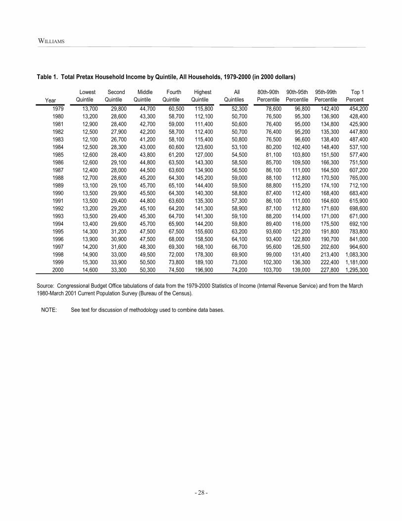
- 28 -
WILLIAMS
Table 1. Total Pretax Household Income by Quintile, All Households, 1979-2000 (in 2000 dollars)
Year Lowest Quintile
Second Quintile
Middle Quintile
Fourth Quintile
Highest Quintile
All Quintiles
80th-90th Percentile
90th-95th Percentile
95th-99th Percentile
Top 1 Percent
1979 13,700 29,800 44,700 60,500 115,800 52,300 78,600 96,800 142,400 454,2001980 13,200 28,600 43,300 58,700 112,100 50,700 76,500 95,300 136,900 428,4001981 12,900 28,400 42,700 59,000 111,400 50,600 76,400 95,000 134,800 425,9001982 12,500 27,900 42,200 58,700 112,400 50,700 76,400 95,200 135,300 447,8001983 12,100 26,700 41,200 58,100 115,400 50,800 76,500 96,600 138,400 487,4001984 12,500 28,300 43,000 60,600 123,600 53,100 80,200 102,400 148,400 537,1001985 12,600 28,400 43,800 61,200 127,000 54,500 81,100 103,800 151,500 577,4001986 12,600 29,100 44,800 63,500 143,300 58,500 85,700 109,500 166,300 751,5001987 12,400 28,000 44,500 63,600 134,900 56,500 86,100 111,000 164,500 607,2001988 12,700 28,600 45,200 64,300 145,200 59,000 88,100 112,800 170,500 765,0001989 13,100 29,100 45,700 65,100 144,400 59,500 88,800 115,200 174,100 712,1001990 13,500 29,900 45,500 64,300 140,300 58,800 87,400 112,400 168,400 683,4001991 13,500 29,400 44,800 63,600 135,300 57,300 86,100 111,000 164,600 615,9001992 13,200 29,200 45,100 64,200 141,300 58,900 87,100 112,800 171,600 698,6001993 13,500 29,400 45,300 64,700 141,300 59,100 88,200 114,000 171,000 671,0001994 13,400 29,600 45,700 65,900 144,200 59,800 89,400 116,000 175,500 692,1001995 14,300 31,200 47,500 67,500 155,600 63,200 93,600 121,200 191,800 783,8001996 13,900 30,900 47,500 68,000 158,500 64,100 93,400 122,800 190,700 841,0001997 14,200 31,600 48,300 69,300 168,100 66,700 95,600 126,500 202,600 964,6001998 14,900 33,000 49,500 72,000 178,300 69,900 99,000 131,400 213,400 1,083,3001999 15,300 33,900 50,500 73,800 189,100 73,000 102,300 136,300 222,400 1,181,0002000 14,600 33,300 50,300 74,500 196,900 74,200 103,700 139,000 227,800 1,295,300
NOTE: See text for discussion of methodology used to combine data bases.
Source: Congressional Budget Office tabulations of data from the 1979-2000 Statistics of Income (Internal Revenue Service) and from the March 1980-March 2001 Current Population Survey (Bureau of the Census).
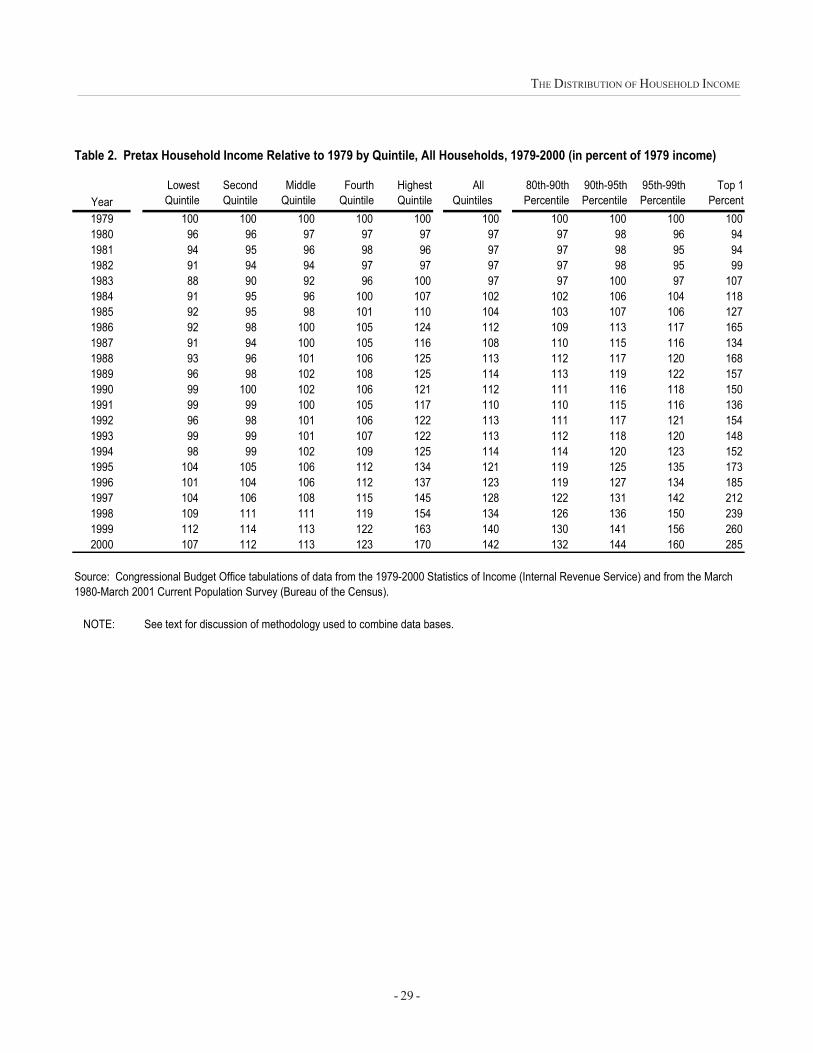
- 29 -
THE DISTRIBUTION OF HOUSEHOLD INCOME
Table 2. Pretax Household Income Relative to 1979 by Quintile, All Households, 1979-2000 (in percent of 1979 income)
Year Lowest
Quintile Second
Quintile Middle
Quintile Fourth
Quintile Highest
Quintile All
Quintiles 80th-90th Percentile
90th-95th Percentile
95th-99th Percentile
Top 1 Percent
1979 100 100 100 100 100 100 100 100 100 1001980 96 96 97 97 97 97 97 98 96 941981 94 95 96 98 96 97 97 98 95 941982 91 94 94 97 97 97 97 98 95 991983 88 90 92 96 100 97 97 100 97 1071984 91 95 96 100 107 102 102 106 104 1181985 92 95 98 101 110 104 103 107 106 1271986 92 98 100 105 124 112 109 113 117 1651987 91 94 100 105 116 108 110 115 116 1341988 93 96 101 106 125 113 112 117 120 1681989 96 98 102 108 125 114 113 119 122 1571990 99 100 102 106 121 112 111 116 118 1501991 99 99 100 105 117 110 110 115 116 1361992 96 98 101 106 122 113 111 117 121 1541993 99 99 101 107 122 113 112 118 120 1481994 98 99 102 109 125 114 114 120 123 1521995 104 105 106 112 134 121 119 125 135 1731996 101 104 106 112 137 123 119 127 134 1851997 104 106 108 115 145 128 122 131 142 2121998 109 111 111 119 154 134 126 136 150 2391999 112 114 113 122 163 140 130 141 156 2602000 107 112 113 123 170 142 132 144 160 285
NOTE: See text for discussion of methodology used to combine data bases.
Source: Congressional Budget Office tabulations of data from the 1979-2000 Statistics of Income (Internal Revenue Service) and from the March 1980-March 2001 Current Population Survey (Bureau of the Census).
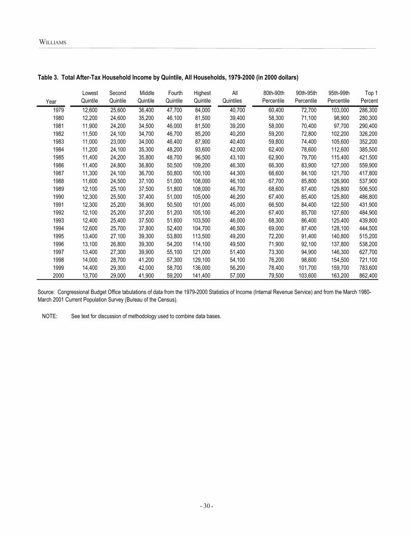
- 30 -
WILLIAMS
Table 3. Total After-Tax Household Income by Quintile, All Households, 1979-2000 (in 2000 dollars)
Year Lowest
Quintile Second
Quintile Middle
Quintile Fourth
Quintile Highest
Quintile All
Quintiles 80th-90th Percentile
90th-95th Percentile
95th-99th Percentile
Top 1 Percent
1979 12,600 25,600 36,400 47,700 84,000 40,700 60,400 72,700 103,000 286,3001980 12,200 24,600 35,200 46,100 81,500 39,400 58,300 71,100 98,900 280,3001981 11,900 24,200 34,500 46,000 81,500 39,200 58,000 70,400 97,700 290,4001982 11,500 24,100 34,700 46,700 85,200 40,200 59,200 72,800 102,200 326,2001983 11,000 23,000 34,000 46,400 87,900 40,400 59,800 74,400 105,600 352,2001984 11,200 24,100 35,300 48,200 93,600 42,000 62,400 78,600 112,600 385,5001985 11,400 24,200 35,800 48,700 96,500 43,100 62,900 79,700 115,400 421,5001986 11,400 24,800 36,800 50,500 109,200 46,300 66,300 83,900 127,000 559,9001987 11,300 24,100 36,700 50,800 100,100 44,300 66,600 84,100 121,700 417,8001988 11,600 24,500 37,100 51,000 108,000 46,100 67,700 85,800 126,900 537,9001989 12,100 25,100 37,500 51,800 108,000 46,700 68,600 87,400 129,800 506,5001990 12,300 25,500 37,400 51,000 105,000 46,200 67,400 85,400 125,800 486,8001991 12,300 25,200 36,900 50,500 101,000 45,000 66,500 84,400 122,500 431,9001992 12,100 25,200 37,200 51,200 105,100 46,200 67,400 85,700 127,600 484,9001993 12,400 25,400 37,500 51,600 103,500 46,000 68,300 86,400 125,400 439,8001994 12,600 25,700 37,800 52,400 104,700 46,500 69,000 87,400 128,100 444,5001995 13,400 27,100 39,300 53,800 113,500 49,200 72,200 91,400 140,800 515,2001996 13,100 26,800 39,300 54,200 114,100 49,500 71,900 92,100 137,800 538,2001997 13,400 27,300 39,900 55,100 121,000 51,400 73,300 94,900 146,300 627,7001998 14,000 28,700 41,200 57,300 129,100 54,100 76,200 98,600 154,500 721,1001999 14,400 29,300 42,000 58,700 136,000 56,200 78,400 101,700 159,700 783,6002000 13,700 29,000 41,900 59,200 141,400 57,000 79,500 103,600 163,200 862,400
NOTE: See text for discussion of methodology used to combine data bases.
Source: Congressional Budget Office tabulations of data from the 1979-2000 Statistics of Income (Internal Revenue Service) and from the March 1980-March 2001 Current Population Survey (Bureau of the Census).

- 31 -
THE DISTRIBUTION OF HOUSEHOLD INCOME
Table 4. After-Tax Household Income Relative to 1979 by Quintile, All Households, 1979-2000 (in percent of 1979 income)
Year Lowest
Quintile Second
Quintile Middle
Quintile Fourth
Quintile Highest
Quintile All
Quintiles 80th-90th Percentile
90th-95th Percentile
95th-99th Percentile
Top 1 Percent
1979 100 100 100 100 100 100 100 100 100 1001980 97 96 97 97 97 97 97 98 96 981981 94 95 95 96 97 96 96 97 95 1011982 91 94 95 98 101 99 98 100 99 1141983 87 90 93 97 105 99 99 102 103 1231984 89 94 97 101 111 103 103 108 109 1351985 90 95 98 102 115 106 104 110 112 1471986 90 97 101 106 130 114 110 115 123 1961987 90 94 101 106 119 109 110 116 118 1461988 92 96 102 107 129 113 112 118 123 1881989 96 98 103 109 129 115 114 120 126 1771990 98 100 103 107 125 114 112 117 122 1701991 98 98 101 106 120 111 110 116 119 1511992 96 98 102 107 125 114 112 118 124 1691993 98 99 103 108 123 113 113 119 122 1541994 100 100 104 110 125 114 114 120 124 1551995 106 106 108 113 135 121 120 126 137 1801996 104 105 108 114 136 122 119 127 134 1881997 106 107 110 116 144 126 121 131 142 2191998 111 112 113 120 154 133 126 136 150 2521999 114 114 115 123 162 138 130 140 155 2742000 109 113 115 124 168 140 132 143 158 301
NOTE: See text for discussion of methodology used to combine data bases.
Source: Congressional Budget Office tabulations of data from the 1979-2000 Statistics of Income (Internal Revenue Service) and from the March 1980-March 2001 Current Population Survey (Bureau of the Census).
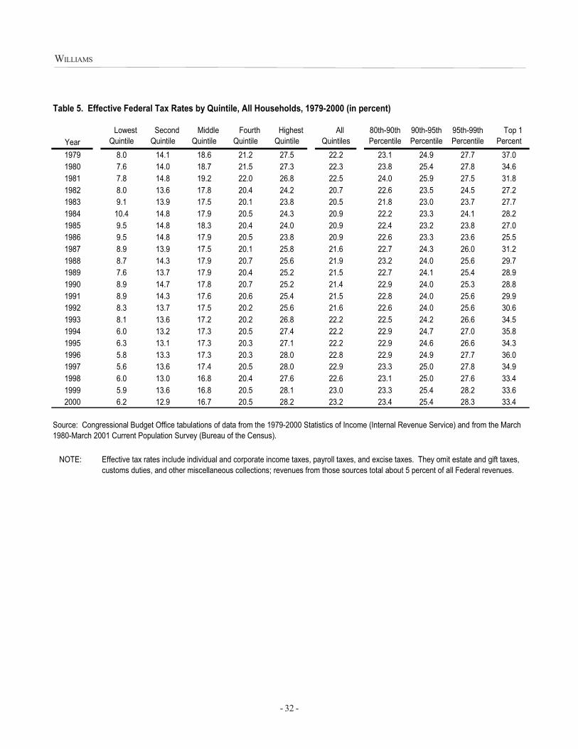
- 32 -
WILLIAMS
Table 5. Effective Federal Tax Rates by Quintile, All Households, 1979-2000 (in percent)
Year Lowest Quintile
Second Quintile
Middle Quintile
Fourth Quintile
Highest Quintile
All Quintiles
80th-90th Percentile
90th-95th Percentile
95th-99th Percentile
Top 1 Percent
1979 8.0 14.1 18.6 21.2 27.5 22.2 23.1 24.9 27.7 37.01980 7.6 14.0 18.7 21.5 27.3 22.3 23.8 25.4 27.8 34.61981 7.8 14.8 19.2 22.0 26.8 22.5 24.0 25.9 27.5 31.81982 8.0 13.6 17.8 20.4 24.2 20.7 22.6 23.5 24.5 27.21983 9.1 13.9 17.5 20.1 23.8 20.5 21.8 23.0 23.7 27.71984 10.4 14.8 17.9 20.5 24.3 20.9 22.2 23.3 24.1 28.21985 9.5 14.8 18.3 20.4 24.0 20.9 22.4 23.2 23.8 27.01986 9.5 14.8 17.9 20.5 23.8 20.9 22.6 23.3 23.6 25.51987 8.9 13.9 17.5 20.1 25.8 21.6 22.7 24.3 26.0 31.21988 8.7 14.3 17.9 20.7 25.6 21.9 23.2 24.0 25.6 29.71989 7.6 13.7 17.9 20.4 25.2 21.5 22.7 24.1 25.4 28.91990 8.9 14.7 17.8 20.7 25.2 21.4 22.9 24.0 25.3 28.81991 8.9 14.3 17.6 20.6 25.4 21.5 22.8 24.0 25.6 29.91992 8.3 13.7 17.5 20.2 25.6 21.6 22.6 24.0 25.6 30.61993 8.1 13.6 17.2 20.2 26.8 22.2 22.5 24.2 26.6 34.51994 6.0 13.2 17.3 20.5 27.4 22.2 22.9 24.7 27.0 35.81995 6.3 13.1 17.3 20.3 27.1 22.2 22.9 24.6 26.6 34.31996 5.8 13.3 17.3 20.3 28.0 22.8 22.9 24.9 27.7 36.01997 5.6 13.6 17.4 20.5 28.0 22.9 23.3 25.0 27.8 34.91998 6.0 13.0 16.8 20.4 27.6 22.6 23.1 25.0 27.6 33.41999 5.9 13.6 16.8 20.5 28.1 23.0 23.3 25.4 28.2 33.62000 6.2 12.9 16.7 20.5 28.2 23.2 23.4 25.4 28.3 33.4
NOTE:
Source: Congressional Budget Office tabulations of data from the 1979-2000 Statistics of Income (Internal Revenue Service) and from the March 1980-March 2001 Current Population Survey (Bureau of the Census).
Effective tax rates include individual and corporate income taxes, payroll taxes, and excise taxes. They omit estate and gift taxes, customs duties, and other miscellaneous collections; revenues from those sources total about 5 percent of all Federal revenues.
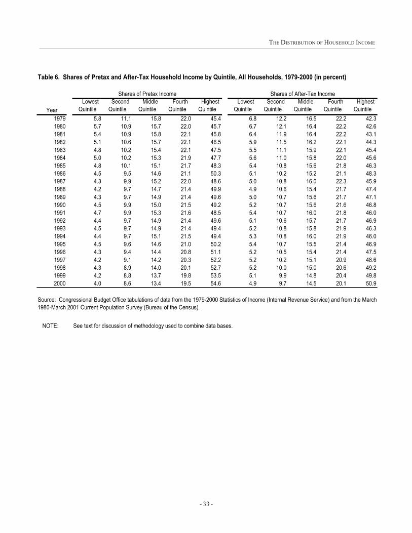
- 33 -
THE DISTRIBUTION OF HOUSEHOLD INCOME
Table 6. Shares of Pretax and After-Tax Household Income by Quintile, All Households, 1979-2000 (in percent)
Year Lowest Quintile
Second Quintile
Middle Quintile
Fourth Quintile
Highest Quintile
Lowest Quintile
Second Quintile
Middle Quintile
Fourth Quintile
Highest Quintile
1979 5.8 11.1 15.8 22.0 45.4 6.8 12.2 16.5 22.2 42.31980 5.7 10.9 15.7 22.0 45.7 6.7 12.1 16.4 22.2 42.61981 5.4 10.9 15.8 22.1 45.8 6.4 11.9 16.4 22.2 43.11982 5.1 10.6 15.7 22.1 46.5 5.9 11.5 16.2 22.1 44.31983 4.8 10.2 15.4 22.1 47.5 5.5 11.1 15.9 22.1 45.41984 5.0 10.2 15.3 21.9 47.7 5.6 11.0 15.8 22.0 45.61985 4.8 10.1 15.1 21.7 48.3 5.4 10.8 15.6 21.8 46.31986 4.5 9.5 14.6 21.1 50.3 5.1 10.2 15.2 21.1 48.31987 4.3 9.9 15.2 22.0 48.6 5.0 10.8 16.0 22.3 45.91988 4.2 9.7 14.7 21.4 49.9 4.9 10.6 15.4 21.7 47.41989 4.3 9.7 14.9 21.4 49.6 5.0 10.7 15.6 21.7 47.11990 4.5 9.9 15.0 21.5 49.2 5.2 10.7 15.6 21.6 46.81991 4.7 9.9 15.3 21.6 48.5 5.4 10.7 16.0 21.8 46.01992 4.4 9.7 14.9 21.4 49.6 5.1 10.6 15.7 21.7 46.91993 4.5 9.7 14.9 21.4 49.4 5.2 10.8 15.8 21.9 46.31994 4.4 9.7 15.1 21.5 49.4 5.3 10.8 16.0 21.9 46.01995 4.5 9.6 14.6 21.0 50.2 5.4 10.7 15.5 21.4 46.91996 4.3 9.4 14.4 20.8 51.1 5.2 10.5 15.4 21.4 47.51997 4.2 9.1 14.2 20.3 52.2 5.2 10.2 15.1 20.9 48.61998 4.3 8.9 14.0 20.1 52.7 5.2 10.0 15.0 20.6 49.21999 4.2 8.8 13.7 19.8 53.5 5.1 9.9 14.8 20.4 49.82000 4.0 8.6 13.4 19.5 54.6 4.9 9.7 14.5 20.1 50.9
NOTE: See text for discussion of methodology used to combine data bases.
Shares of Pretax Income Shares of After-Tax Income
Source: Congressional Budget Office tabulations of data from the 1979-2000 Statistics of Income (Internal Revenue Service) and from the March 1980-March 2001 Current Population Survey (Bureau of the Census).
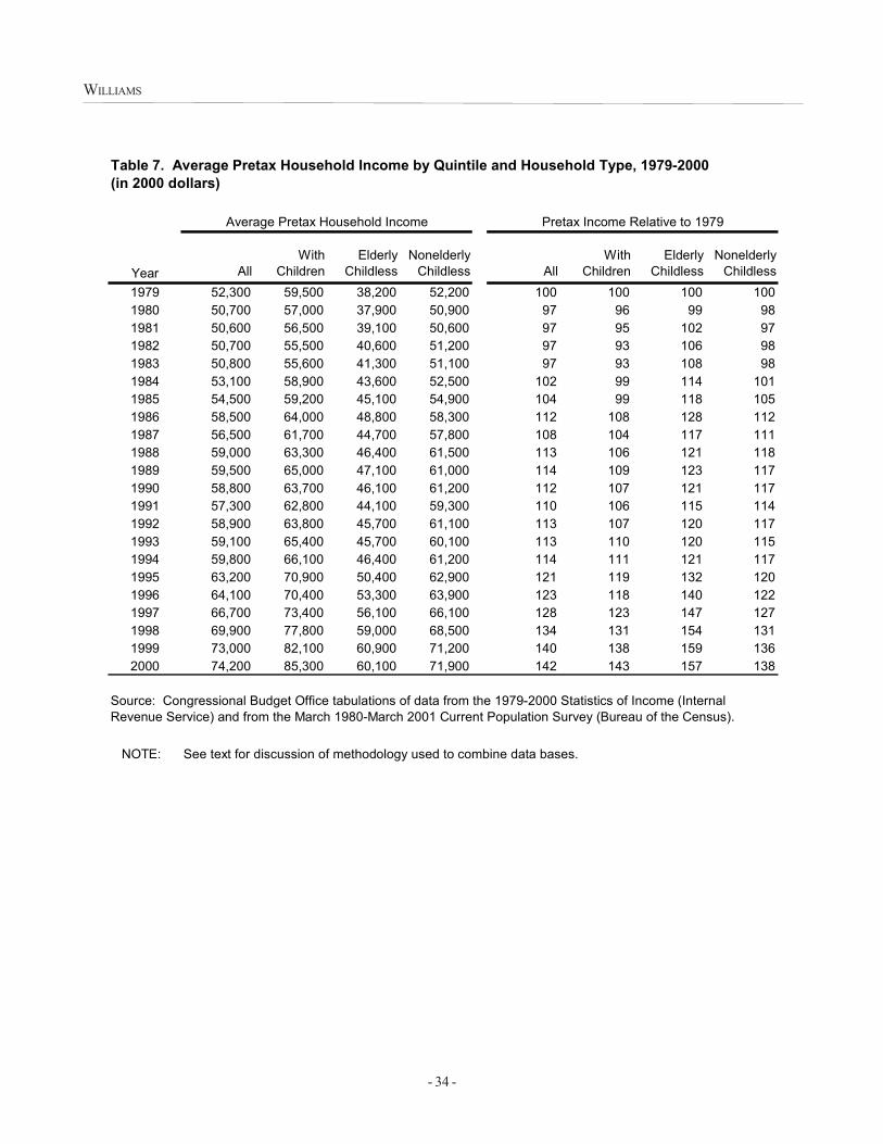
- 34 -
WILLIAMS
Table 7. Average Pretax Household Income by Quintile and Household Type, 1979-2000 (in 2000 dollars)
Year AllWith
ChildrenElderly
ChildlessNonelderly
Childless AllWith
ChildrenElderly
ChildlessNonelderly
Childless1979 52,300 59,500 38,200 52,200 100 100 100 1001980 50,700 57,000 37,900 50,900 97 96 99 981981 50,600 56,500 39,100 50,600 97 95 102 971982 50,700 55,500 40,600 51,200 97 93 106 981983 50,800 55,600 41,300 51,100 97 93 108 981984 53,100 58,900 43,600 52,500 102 99 114 1011985 54,500 59,200 45,100 54,900 104 99 118 1051986 58,500 64,000 48,800 58,300 112 108 128 1121987 56,500 61,700 44,700 57,800 108 104 117 1111988 59,000 63,300 46,400 61,500 113 106 121 1181989 59,500 65,000 47,100 61,000 114 109 123 1171990 58,800 63,700 46,100 61,200 112 107 121 1171991 57,300 62,800 44,100 59,300 110 106 115 1141992 58,900 63,800 45,700 61,100 113 107 120 1171993 59,100 65,400 45,700 60,100 113 110 120 1151994 59,800 66,100 46,400 61,200 114 111 121 1171995 63,200 70,900 50,400 62,900 121 119 132 1201996 64,100 70,400 53,300 63,900 123 118 140 1221997 66,700 73,400 56,100 66,100 128 123 147 1271998 69,900 77,800 59,000 68,500 134 131 154 1311999 73,000 82,100 60,900 71,200 140 138 159 1362000 74,200 85,300 60,100 71,900 142 143 157 138
NOTE: See text for discussion of methodology used to combine data bases.
Average Pretax Household Income Pretax Income Relative to 1979
Source: Congressional Budget Office tabulations of data from the 1979-2000 Statistics of Income (Internal Revenue Service) and from the March 1980-March 2001 Current Population Survey (Bureau of the Census).
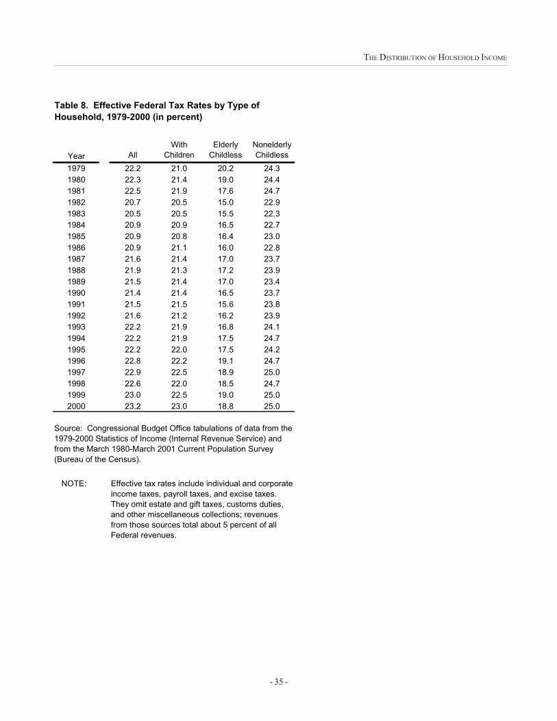
- 35 -
THE DISTRIBUTION OF HOUSEHOLD INCOME
Year AllWith
ChildrenElderly
ChildlessNonelderly Childless
1979 22.2 21.0 20.2 24.31980 22.3 21.4 19.0 24.41981 22.5 21.9 17.6 24.71982 20.7 20.5 15.0 22.91983 20.5 20.5 15.5 22.31984 20.9 20.9 16.5 22.71985 20.9 20.8 16.4 23.01986 20.9 21.1 16.0 22.81987 21.6 21.4 17.0 23.71988 21.9 21.3 17.2 23.91989 21.5 21.4 17.0 23.41990 21.4 21.4 16.5 23.71991 21.5 21.5 15.6 23.81992 21.6 21.2 16.2 23.91993 22.2 21.9 16.8 24.11994 22.2 21.9 17.5 24.71995 22.2 22.0 17.5 24.21996 22.8 22.2 19.1 24.71997 22.9 22.5 18.9 25.01998 22.6 22.0 18.5 24.71999 23.0 22.5 19.0 25.02000 23.2 23.0 18.8 25.0
NOTE:
Table 8. Effective Federal Tax Rates by Type of Household, 1979-2000 (in percent)
Source: Congressional Budget Office tabulations of data from the 1979-2000 Statistics of Income (Internal Revenue Service) and from the March 1980-March 2001 Current Population Survey (Bureau of the Census).
Effective tax rates include individual and corporate income taxes, payroll taxes, and excise taxes. They omit estate and gift taxes, customs duties, and other miscellaneous collections; revenues from those sources total about 5 percent of all Federal revenues.
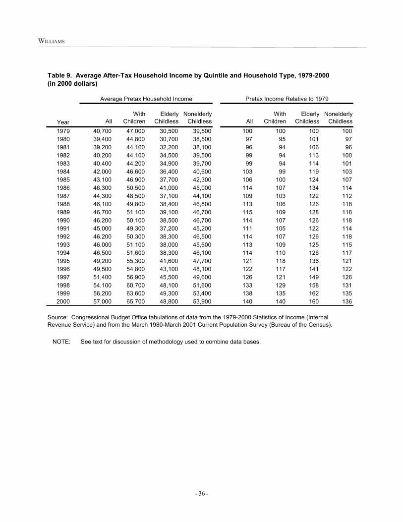
- 36 -
WILLIAMS
Table 9. Average After-Tax Household Income by Quintile and Household Type, 1979-2000 (in 2000 dollars)
Year AllWith
ChildrenElderly
ChildlessNonelderly
Childless AllWith
ChildrenElderly
ChildlessNonelderly
Childless1979 40,700 47,000 30,500 39,500 100 100 100 1001980 39,400 44,800 30,700 38,500 97 95 101 971981 39,200 44,100 32,200 38,100 96 94 106 961982 40,200 44,100 34,500 39,500 99 94 113 1001983 40,400 44,200 34,900 39,700 99 94 114 1011984 42,000 46,600 36,400 40,600 103 99 119 1031985 43,100 46,900 37,700 42,300 106 100 124 1071986 46,300 50,500 41,000 45,000 114 107 134 1141987 44,300 48,500 37,100 44,100 109 103 122 1121988 46,100 49,800 38,400 46,800 113 106 126 1181989 46,700 51,100 39,100 46,700 115 109 128 1181990 46,200 50,100 38,500 46,700 114 107 126 1181991 45,000 49,300 37,200 45,200 111 105 122 1141992 46,200 50,300 38,300 46,500 114 107 126 1181993 46,000 51,100 38,000 45,600 113 109 125 1151994 46,500 51,600 38,300 46,100 114 110 126 1171995 49,200 55,300 41,600 47,700 121 118 136 1211996 49,500 54,800 43,100 48,100 122 117 141 1221997 51,400 56,900 45,500 49,600 126 121 149 1261998 54,100 60,700 48,100 51,600 133 129 158 1311999 56,200 63,600 49,300 53,400 138 135 162 1352000 57,000 65,700 48,800 53,900 140 140 160 136
NOTE: See text for discussion of methodology used to combine data bases.
Average Pretax Household Income Pretax Income Relative to 1979
Source: Congressional Budget Office tabulations of data from the 1979-2000 Statistics of Income (Internal Revenue Service) and from the March 1980-March 2001 Current Population Survey (Bureau of the Census).
- 37 -
Comments on Papers by Welniak; Strudler, Petska,and Petska; and Williams ¹
Eric. J. Toder, Internal Revenue Service
T hese three papers by analysts at the U.S. Bu-reau of the Census, the Statistics of Income (SOI)Division of the Internal Revenue Service, and the
Congressional Budget Office (CBO) estimate changesin the distribution of income over the past two decades.In my remarks, I first address what the three papershave in common. Then, I discuss some of the main is-sues in measuring the distribution of income and com-pare how these three papers addressed these issues. Icomment on the strengths and weaknesses of alterna-tive approaches. Finally, I briefly discuss some implica-tions of the authors� findings. For brevity, I referencethe papers in the discussion by the institutional affilia-tions of the authors (Census, SOI, and CBO).
� Common Features of the Three Papers
All the papers measure changes in the distributionof income over the past two decades. Census estimateschanges in the distribution of pretax income between1979 and 2000 and also extends its analysis back to 1967.SOI estimates changes in the distribution of pretax andpost-tax income between 1979 and 2001. CBO looks atthe changes in a broader measure of pretax income thatincludes taxes paid by businesses between 1979 and 2000.
All the papers show that inequality has increasedover the past two decades. Census shows that Ginicoefficients and other commonly used inequality mea-sures have increased. SOI shows that pretax and post-tax Gini coefficients have increased, that income cut-offs at the top percentiles of the income distribution haveincreased faster than income cutoffs for lower percen-tile groupings, and that the share of income going to thehighest percentiles of the population has also increased.CBO shows that average pretax income has grownfaster for the higher percentile groupings than for otherpopulation groups.
All three papers compare �snapshots� of the incomedistribution in different years. That is, they comparedispersions of income among samples of the population,
but the individuals in the sample change over time. Thus,none of the studies is examining changes over time inthe incomes of a fixed group of individuals, as would bedone by a panel study. An alternative and more concep-tually appealing way to look at income distribution is tomeasure the dispersion of lifetime incomes across a fixedpopulation, but available data do not facilitate comparinghow the dispersion of lifetime incomes changes over time.Compared with a distribution of lifetime incomes, the�snapshot� distributions in these papers overstate inequal-ity for two reasons. First, they include some individualswhose incomes are temporarily high or low in a givenyear because of, for example, windfall gains or a spell ofunemployment. Second, they include individuals at dif-ferent ages; so, a portion of the inequality reflects thevariation in incomes over a person�s lifecycle and notlifetime difference in incomes among people. While thepapers overstate the level of inequality, however, it doesnot follow that they overstate the increase in inequality.
� Methodological Issues in MeasuringIncome Distribution and How PapersAddress Them
While the papers reach similar conclusions, they dif-fer significantly in their approaches. This reflects thenumerous methodological issues that researchers con-front in measuring income distribution. The differencesin part also reflect differences in the types of data pro-duced by the agencies where the researchers work. Inthis section, I discuss the strengths and weaknesses ofdifferent approaches and compare the choices made inthe three papers.
Choice of an Income Concept. The first ques-tion is what income concept to use, given the existenceof taxes and Government transfer programs. The twoconceptually pure alternatives are to look at income thatpeople receive from market transactions�that is, incomein the absence of Government taxes and transfers�orto look at income net of all Government taxes and trans-fers. The latter is the best measure of the well-being of
- 38 -
TODER
individuals, while the distribution of market income indi-cates how the income distribution might have changed,absent changes in the tax law.
None of the authors estimates the distribution ofmarket income, while only CBO displays changes net ofFederal Government taxes and transfers.2 Instead, CBOmeasures income before taxes but including transfers,while Census and SOI measure income before individualincome taxes but net of business taxes. SOI also mea-sures income net of taxes, while CBO measures incomenet of both taxes and transfers.
Measuring pretax income is not straightforward. Weobserve reported income of individuals before taxes, butwe do not really know whose incomes are reduced howmuch by taxes. In the case of the individual income tax,it is typical, though not strictly correct, for researchersto assume that the tax reduces the after-tax incomes ofthose who pay it, but does not affect anyone�s observedpretax income.3 But there are differing views on whichindividuals experience lower after-tax incomes as a re-sult of taxes remitted by businesses. CBO allocates theemployer portion of payroll taxes in proportion to wagesreceived, and the corporate income tax in proportion toinvestment income (interest, dividends, capital gains) ofindividuals, and adds these taxes back to observed in-come to derive its measure of pretax income. Theseare reasonable assumptions, but not the only possibleones.
Inclusiveness of Income Measure. Economicincome is defined as the sum of consumption plus changesin net worth. By this broad measure, income includes allsources of cash receipts, net of costs of earning in-come�wages, interest, dividends, rents, and businessprofits�plus changes in the value of assets (adjustedfor inflation), income from noncash fringe benefits, andthe net imputed value of consumption services from du-rable goods (principally houses). None of the authorsuses this broad a measure of income, although the U.S.Treasury Department has used such a measure (called�family economic income�) in analyses of the distribu-tional effect of Federal taxes. See Cronin (1999).
All the authors include cash flow income (wages,interest, dividends, rent, profits) in their income measures.
CBO, as noted above, also adds back business taxes toarrive at a broader measure of pretax income. No onecounts accrued capital gains or other forms of accruedincome (such as the inside buildup on pensions and lifeinsurance reserves), but CBO and SOI include realizedgains reported on tax returns. CBO and Census includecash transfer payments in their measures, but SOI doesnot. CBO also imputes some in-kind benefits received,such as the value of employer-provided health insurance.
Making the income measure broader improves it asa measure of economic well-being, but can come at acost for items not reported in the primary data source(see below), but imputed from other data sets. Research-ers confront a tradeoff between the quality of the in-come concept and the precision of the data.
Unit of Measurement. Another issue is how todefine the unit of comparison. Because people who arerelated or live together typically pool their incomes, mostresearchers do not examine the distribution of incomeacross individuals. Census and CBO use the house-hold as their unit of analysis, while SOI uses tax filingunits. In general, comparing incomes across householdsis preferable to comparison across tax units for two rea-sons. First, tax units exclude nonfilers, and thereforemiss many households at the low end of the income dis-tribution (although they do include low-income peoplewithout a filing requirement who file a return to get re-funds of withheld taxes or to claim refundable credits.)Second, tax units include some individuals, such as manystudents, whose economic well-being is represented bet-ter by the incomes of their families than by their indi-vidual incomes.
A related issue, if the household or family is the unitof measure, is if and how to adjust for differences infamily size. The same income supports differing stan-dards of living for households of different compositions,and changes in the composition of households (by mari-tal status and household size) over time can affect trendsin measures of income distribution. Among the authors,only CBO includes an explicit adjustment for family sizein the analysis. CBO also reports trends in income distri-bution within more homogenous subgroups�elderly child-less households, nonelderly childless households, andhouseholds with children. In particular, they find that
- 39 -
COMMENTS ON PAPERS BY WELNIAK; STRUDLER, PETSKA, AND PETSKA; AND WILLIAMS
incomes of elderly childless households have increasedmore over the past two decades than incomes of otherhousehold types.
Sources of Data. Not surprisingly, the authors usethe sources of data their agencies produce�Census usesdata from their Current Population Survey (CPS), whileSOI uses administrative tax data from a sample of indi-vidual tax returns. CBO performs a statistical matchbetween CPS and SOI data; the CPS sample is used asthe basis for the CBO households, while SOI data arethe basis for estimated incomes.
Each approach has strengths and weaknesses.Typically, administrative data are more accurate andcomplete than survey data; in particular, income fromcapital reported on tax returns is much larger than in-come from capital reported to CPS and much closer tototals in the National Income and Product Accounts. ButSOI data are limited to what people are required to re-port on their tax returns, while the CPS collects a broaderrange of data and includes a representative nationalsample of households, not just tax filers. (SOI does in-clude data on realized capital gains, which are not col-lected by Census.) CBO attempts to get the best ofboth worlds by merging tax return and CPS data, but theuse of statistical matching procedures means that incomesare in part estimated rather than observed.
Measures of Inequality. Finally, the researchersuse different indices to measure inequality. SOI andCBO (but not Census) examine changes in income sharesamong percentile groups. SOI also measures changesin the income levels at which percentile breaks begin.Both Census and SOI, but not CBO, estimate changesin the �Gini� coefficient, a commonly used overall indexof inequality. Census also reports alternative summarymeasures that apply different weights to different partsof the income distribution. SOI and CBO, but not Cen-sus, compare changes in pre- and post-tax measures ofinequality. In spite of this diversity, all the measures usedshow rising inequality over the past two decades.
� Concluding Comments
These are excellent papers and good examples ofthe careful and high-quality research performed within
U.S. Government agencies. While the authors addressdifficult methodological issues in diverse ways, they reachbroadly similar conclusions about trends in income dis-tribution. Using measures of annual income, the disper-sion of income has clearly increased. While this doesnot definitively establish that the distribution of lifetimeincome has become less equal, it certainly provides causefor concern about widening inequality in the United States.
How much this all has to do with Government fiscalpolicies, however, is not clear. Inequality widened in the1980�s, as tax rates, especially on high-income individu-als, were falling. Inequality also widened in the 1990�s,when tax rates on high-income individuals were in-creased. Since 2001, in the face of new tax cuts, mea-sures of inequality may be narrowing as a result of therecent decline in stock prices, which disproportionatelyaffects reported incomes (especially from capital gains)of high-income individuals. This suggests that tax poli-cies, while modifying market outcomes, are probably notthe major driver of the changes in income distribution.
� Notes and References
1 See Welniak (2003); Strudler, Petska, and Petska(2003); and Williams (2003), this volume.
2 The CBO measure does not include the effects ofState and local taxes and transfers.
3 This assumption is a good approximation, but doesnot hold in all cases. For example, tax-exemptmunicipal bonds pay lower interest rates than tax-able securities of comparable risk. Recipients ofincome from tax-exempt bonds do not pay taxes tothe Federal Government, but do receive lower in-comes from those securities than they would have,absent a Federal income tax.
Cronin, Julie-Anne (1999), �U.S. Treasury Distribu-tional Analysis Methodology,� OTA Paper 85(September).
Strudler, Michael; Petska, Tom; and Petska, Ryan(2003), �An Analysis of the Distribution of Indi-vidual Income and Taxes, 1979-2001, presented atthe Joint Statistical Meetings, San Francisco,California (August).

- 40 -
TODER
Welniak, Edward J. (2003), �Measuring HouseholdInequality Using the CPS,� presented at theJoint Statistical Meetings, San Francisco, Califor-nia (August).
Williams, Roberton C., Jr. (2003), �The Distribution ofHousehold Income: Two Decades of Change,�presented at the Joint Statistical Meetings, SanFrancisco, California, (August).
�
2
Recent Developmentin Survey Methods
Wong Ho�
- 43 -
Comparing Scoring Systems From Cluster Analysisand Discriminant Analysis Using Random Samples
William Wong and Chih-Chin Ho, Internal Revenue Service
C urrently, the Internal Revenue Service (IRS) cal-culates a scoring formula for each tax return anduses it as one criterion to determine which re-
turns to audit. The IRS periodically updates this formulafrom a stratified random audit sample. In 1988, such anaudit sample was selected. The sample was used to de-rive a new scoring formula. This score is one of thecriteria used to determine whom to audit. In Wong andHo (2002), we examined the effect of changing samplesize on the scoring formula from discriminant analysis.We now extend that work by examining a method ofderiving scoring functions using cluster analysis with avariety of distance functions and other options. Thoseresults are compared, and the best results are then com-pared against those from discriminant analysis. For theevaluation, random subsamples of edited returns are se-lected, scoring functions developed and applied, and av-erage performances and variances calculated.
We discuss the design of our analysis, our data, andour goals. We then describe our cluster analysis anddiscriminant analysis approaches. The results of ouranalysis are presented, with the associated tables in theAppendix. Finally, we highlight our conclusions and fu-ture research.
� Basic Analysis Framework
We studied one examination class with a sample of4,356 audited returns. For our study purposes, we se-lected a fixed set of 100 original variables. For the clus-ter analysis procedures, we primarily used a fixed sub-set of 15 of the �best� variables. We also compared us-ing the 15 �best� variables with using the full set of 100variables in the cluster procedure. In the discriminantanalysis procedures, for each random subsample, weused SAS Proc Stepdisc to determine a subset of the100 variables to use to create our discriminant function.We used a cross-validation approach to evaluate theperformances of the scoring formulas.
We start by selecting stratified random subsamplesof 2,500 from our 4,356 sample returns using three strata.These subsamples of 2,500 returns serve as the model-ing data sets. Thus, for each of these subsamples, wecreate the cluster analysis and/or discriminant analysismodels we wish to compare. Our modeling goal is tomaximize the likelihood of identifying returns that ex-ceed a minimum threshold discrepancy between the re-ported and audited tax amounts. (Due to disclosure sen-sitivity, the threshold dollar amount is withheld.) Wenow apply the resulting models on the test data sets ofthe remaining 1,856 (= 4,356 - 2,500) returns to scoreeach return. Here, a higher score means the model ispredicting a higher probability of the return achievingthe threshold. The test data set returns are sorted bydescending scores, and a cutoff percentage, c, of re-turns is selected for evaluation. The evaluation statistic,the �hit rate,� is defined as the portion of the selectedweighted returns achieving the threshold. Cutoff per-centages of 1, 2, 3, 4, 5, 6, 7, 8, 9, 10, 15, 20, 25, 30, 35,40, 45, 50, and 75 are analyzed. The cutoff percentageof 100 is also tabulated to provide the average hit ratesover the entire test data sets. This procedure is re-peated by reselecting 10 to 400 random subsamples,modeling, calculating hit rates for each cutoff percent-age, averaging the hit rates over the subsamples, andcalculating the variance of each average hit rate.
� Cluster Analysis Framework
Motivation: Our approach is to identify returns thatexceed the discrepancy threshold, find where they clus-ter, and score the returns based on their shortest dis-tance to the cluster centroids.
Our cluster analysis proceeds as follows:
� Obtain modeling data set: Select a stratified ran-dom subsample of 2,500 of the 4,356 returns.
- 44 -
WONG AND HO
� Identify those returns that exceeded the thresh-old tax discrepancy. Typically, this would bearound 10 percent of the subsample.
� Create clusters of these �threshold exceeders�:Using those returns that exceed the thresholdtax discrepancy, run SAS Proc Cluster to cre-ate clusters. To create these clusters, we usemost of the distance functions available in SASProc Cluster: average, centroid, complete,EML, flexible, McQuitty, median, single, andWard. Distance functions average, centroid,median, and Ward also have �nosquare� op-tions where the distances are not squared.
� Find the centroids of each cluster: For eachcluster, obtain the means and standard devia-tions for each variable.
� Develop raw predicted score functions: Foreach return exceeding the threshold, calculateits standardized distance to each cluster cen-troid. Thus, for each variable, calculate thedistance between the return value and the clus-ter mean and divide the result by the clusterstandard deviation. Define the distance to eachcluster centroid to be the square root of thesum of the squares of the distances across vari-ables. The minimum of these distances acrossclusters is the raw predicted score. (When acluster�s average standard deviation is zero, thevariable mean with a minimum of one is used.)
� Create cluster score adjustment factors: Foreach cluster, obtain both its average raw pre-dicted score and its average real score, the taxdiscrepancy among its elements. The adjustedpredicted score is then the raw score with a ratioadjustment to even out the cluster-to-cluster differ-ences and prorate to the real score averages.
� Obtain the test data set: The test data set is theremaining 1,856 (= 4,356-2,500) returns.
� Score each test data set return: For each re-turn, calculate raw scores using the same pro-cedure as above and then apply the adjustment
factors calculated above. Since a lower scorecurrently means a higher likelihood of exceed-ing the threshold, the scores need to be inverted.Since the scores are used only in ranking re-turns, simply reverse the sort.
� Calculate hit rates for each cutoff percentage:After sorting the returns, apply the strata sam-pling weights to each return and calculate theweighted hit rates for each cutoff percentage.
� Select the next random subsample and repeatthe procedure 10 or 400 times.
� Calculate average hit rates and standard de-viations over the random subsamples.
� Discriminant Analysis Framework
For our study purposes, we selected 100 originalvariables and used SAS Proc Stepdisc to determine whichvariables to use for our discriminant function. Thus, the100 variables are fixed, but the resulting subset of vari-ables changes from sample to sample. The discrimina-tion classification variable used is a zero-one indicatorof whether a return exceeds the threshold tax discrepancy.
We start by selecting stratified subsamples of 2,500from the 4,356 returns using three strata. The weightedsamples are first processed through SAS Proc Stepdiscto determine which subset of variables will be used. Thisis done using two methods: stepwise with p=0.15 andforward discrimination with a maximum of 15 variables.The weighted subsamples are then processed throughSAS Proc Discrim using only the variables identified bythe Proc Stepdisc procedure. Only parametric discrimi-nation is tested. These weighted subsamples serve asthe discrimination modeling data set. The discriminationtest data set is the remaining 1,856 (=4,356-2,500) re-turns. One output of Proc Discrim is the posterior prob-ability of the test return exceeding the threshold. Thisposterior probability is used as the score. The test dataset returns are sorted by descending scores and weighted,and hit rates are calculated for each cutoff percentage.This procedure is repeated over the 400 randomsubsamples, and average hit rates and their variancesare calculated.
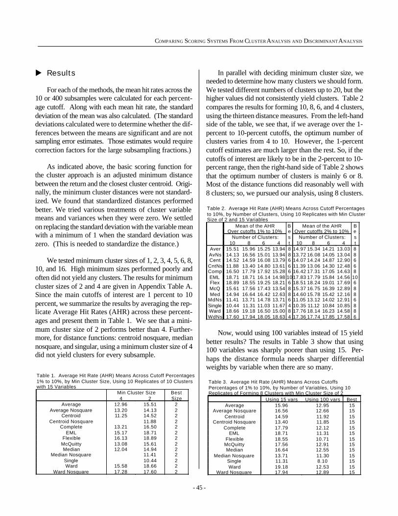
- 45 -
COMPARING SCORING SYSTEMS FROM CLUSTER ANALYSIS AND DISCRIMINANT ANALYSIS
u Results
For each of the methods, the mean hit rates across the10 or 400 subsamples were calculated for each percent-age cutoff. Along with each mean hit rate, the standarddeviation of the mean was also calculated. (The standarddeviations calculated were to determine whether the dif-ferences between the means are significant and are notsampling error estimates. Those estimates would requirecorrection factors for the large subsampling fractions.)
As indicated above, the basic scoring function forthe cluster approach is an adjusted minimum distancebetween the return and the closest cluster centroid. Origi-nally, the minimum cluster distances were not standard-ized. We found that standardized distances performedbetter. We tried various treatments of cluster variablemeans and variances when they were zero. We settledon replacing the standard deviation with the variable meanwith a minimum of 1 when the standard deviation waszero. (This is needed to standardize the distance.)
We tested minimum cluster sizes of 1, 2, 3, 4, 5, 6, 8,10, and 16. High minimum sizes performed poorly andoften did not yield any clusters. The results for minimumcluster sizes of 2 and 4 are given in Appendix Table A.Since the main cutoffs of interest are 1 percent to 10percent, we summarize the results by averaging the rep-licate Average Hit Rates (AHR) across these percent-ages and present them in Table 1. We see that a mini-mum cluster size of 2 performs better than 4. Further-more, for distance functions: centroid nosquare, mediannosquare, and singular, using a minimum cluster size of 4did not yield clusters for every subsample.
In parallel with deciding minimum cluster size, weneeded to determine how many clusters we should form.We tested different numbers of clusters up to 20, but thehigher values did not consistently yield clusters. Table 2compares the results for forming 10, 8, 6, and 4 clusters,using the thirteen distance measures. From the left-handside of the table, we see that, if we average over the 1-percent to 10-percent cutoffs, the optimum number ofclusters varies from 4 to 10. However, the 1-percentcutoff estimates are much larger than the rest. So, if thecutoffs of interest are likely to be in the 2-percent to 10-percent range, then the right-hand side of Table 2 showsthat the optimum number of clusters is mainly 6 or 8.Most of the distance functions did reasonably well with8 clusters; so, we pursued our analysis, using 8 clusters.
Table 1. Average Hit Rate (AHR) Means Across Cutoff Percentages 1% to 10%, by Min Cluster Size, Using 10 Replicates of 10 Clusters with 15 Variables
Min Cluster Size Best 4 2 Size
Average 12.96 15.51 2 Average Nosquare 13.20 14.13 2
Centroid 11.25 14.52 2 Centroid Nosquare 11.88 2
Complete 13.21 16.50 2 EML 15.17 18.71 2
Flexible 16.13 18.89 2 McQuitty 13.08 15.61 2 Median 12.04 14.94 2
Median Nosquare 11.41 2 Single 10.44 2 Ward 15.58 18.66 2
Ward Nosquare 17.28 17.60 2
Table 2. Average Hit Rate (AHR) Means Across Cutoff Percentages to 10%, by Number of Clusters, Using 10 Replicates with Min Cluster Size of 2 and 15 Variables
Mean of the AHR B Mean of the AHR B Over cutoffs 1% to 10% e Over cutoffs 2% to 10% e Number of Clusters: s Number of Clusters: s 10 8 6 4 t 10 8 6 4 t
Aver 15.51 15.96 15.25 13.94 8 14.97 15.34 14.21 13.03 8 AvNs 14.13 16.56 15.01 13.94 8 13.72 16.08 14.05 13.04 8 Cent 14.52 14.59 16.08 13.79 6 14.07 14.24 14.87 12.90 6
CntNs 11.88 13.40 14.80 13.61 6 11.39 13.06 14.30 12.48 6 Comp 16.50 17.79 17.92 15.28 6 16.42 17.31 17.05 14.63 8 EML 18.71 18.71 16.14 14.98 10 17.83 17.79 15.84 14.56 10 Flex 18.89 18.55 19.25 18.21 6 18.51 18.24 19.01 17.69 6 McQ 15.61 17.56 17.43 13.54 8 15.37 16.75 16.39 12.89 8 Med 14.94 16.64 16.42 12.63 8 14.60 15.78 15.42 12.16 8
MdNs 11.41 13.71 14.78 13.71 6 11.05 13.12 14.02 12.91 6 Single 10.44 11.31 11.03 11.67 4 10.35 11.12 10.84 10.85 8 Ward 18.66 19.18 16.50 15.00 8 17.76 18.14 16.23 14.58 8 WdNs 17.60 17.94 18.05 18.63 4 17.36 17.74 17.85 17.58 6
Now, would using 100 variables instead of 15 yield
better results? The results in Table 3 show that using100 variables was sharply poorer than using 15. Per-haps the distance formula needs sharper differentialweights by variable when there are so many.
Table 3. Average Hit Rate (AHR) Means Across Cutoffs Percentages of 1% to 10%, by Number of Variables, Using 10 Replicates of Forming 8 Clusters with Min Cluster Size of 2
Using 15 vars Using 100 vars Best Average 15.96 12.95 15
Average Nosquare 16.56 12.66 15 Centroid 14.59 11.92 15
Centroid Nosquare 13.40 11.85 15 Complete 17.79 12.12 15
EML 18.71 11.31 15 Flexible 18.55 10.71 15
McQuitty 17.56 12.91 15 Median 16.64 12.55 15
Median Nosquare 13.71 11.30 15 Single 11.31 8.10 15 Ward 19.18 12.53 15
Ward Nosquare 17.94 12.89 15
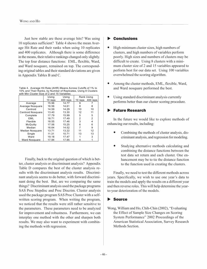
- 46 -
WONG AND HO
Just how stable are these average hits? Was using10 replicates sufficient? Table 4 shows the mean Aver-age Hit Rate and their ranks when using 10 replicatesand 400 replicates. Although there is some differencein the means, their relative rankings changed only slightly.The top four distance functions: EML, flexible, Ward,and Ward nosquare, remained on top. The correspond-ing original tables and their standard deviations are givenin Appendix Tables B and C.
Table 4. Average Hit Rate (AHR) Means Across Cutoffs of 1% to 10% and Their Ranks, by Number of Replicates, Using 8 Clusters with Min Cluster Size of 2 and 15 Variables
Using Using Rank Using 10 reps 400 reps 10 reps 400 reps
Average 15.96 14.77 9 7 Average Nosquare 16.56 14.61 8 8
Centroid 14.59 14.29 10 10 Centroid Nosquare 13.40 13.30 12 11
Complete 17.79 15.99 5 5 EML 18.71 17.49 2 2
Flexible 18.55 17.46 3 4 McQuitty 17.56 15.25 6 6 Median 16.64 14.52 7 9
Median Nosquare 13.71 13.22 11 12 Single 11.31 10.71 13 13 Ward 19.18 17.47 1 3
Ward Nosquare 17.94 17.95 4 1
Finally, back to the original question of which is bet-ter, cluster analysis or discriminant analysis? AppendixTable D compares the best of the cluster analysis re-sults with the discriminant analysis results. Discrimi-nant analysis seems to do better, with forward discrimi-nant doing the best. But, are we comparing the samethings? Discriminant analysis used the package programsSAS Proc Stepdisc and Proc Discrim. Cluster analysisused the package program SAS Proc Cluster with a self-written scoring program. When writing the program,we noticed that the results were still rather sensitive tothe parameters. These parameters need to be analyzedfor improvement and robustness. Furthermore, we caninterplay one method with the other and sharpen bothresults. We may also want to experiment with combin-ing the methods with regression.
� Conclusions
� High minimum cluster sizes, high numbers ofclusters, and high numbers of variables performpoorly. High sizes and numbers of clusters may bedifficult to create. Using 8 clusters with a mini-mum cluster size of 2 and 15 variables appeared toperform best for our data set. Using 100 variablesoverwhelmed the scoring algorithm.
� Among the cluster methods, EML, flexible, Ward,and Ward nosquare performed the best.
� Using standard discriminant analysis currentlyperforms better than our cluster scoring procedure.
� Future Research
In the future we would like to explore methods ofenhancing our results, including:
� Combining the methods of cluster analysis, dis-criminant analysis, and regression for modeling.
� Studying alternative methods calculating andcombining the distance functions between thetest data set return and each cluster. One en-hancement may be to tie the distance functionto the function used in creating the clusters.
Finally, we need to test the different methods acrossyears. Specifically, we wish to use one year�s data totrain the models and apply the results on a different yearand then reverse roles. This will help determine the year-to-year deterioration of the models.
� Source
Wong, William and Ho, Chih-Chin (2002), �Evaluatingthe Effect of Sample Size Changes on ScoringSystem Performance� 2002 Proceedings of theAmerican Statistical Association, Survey ResearchMethods Section.
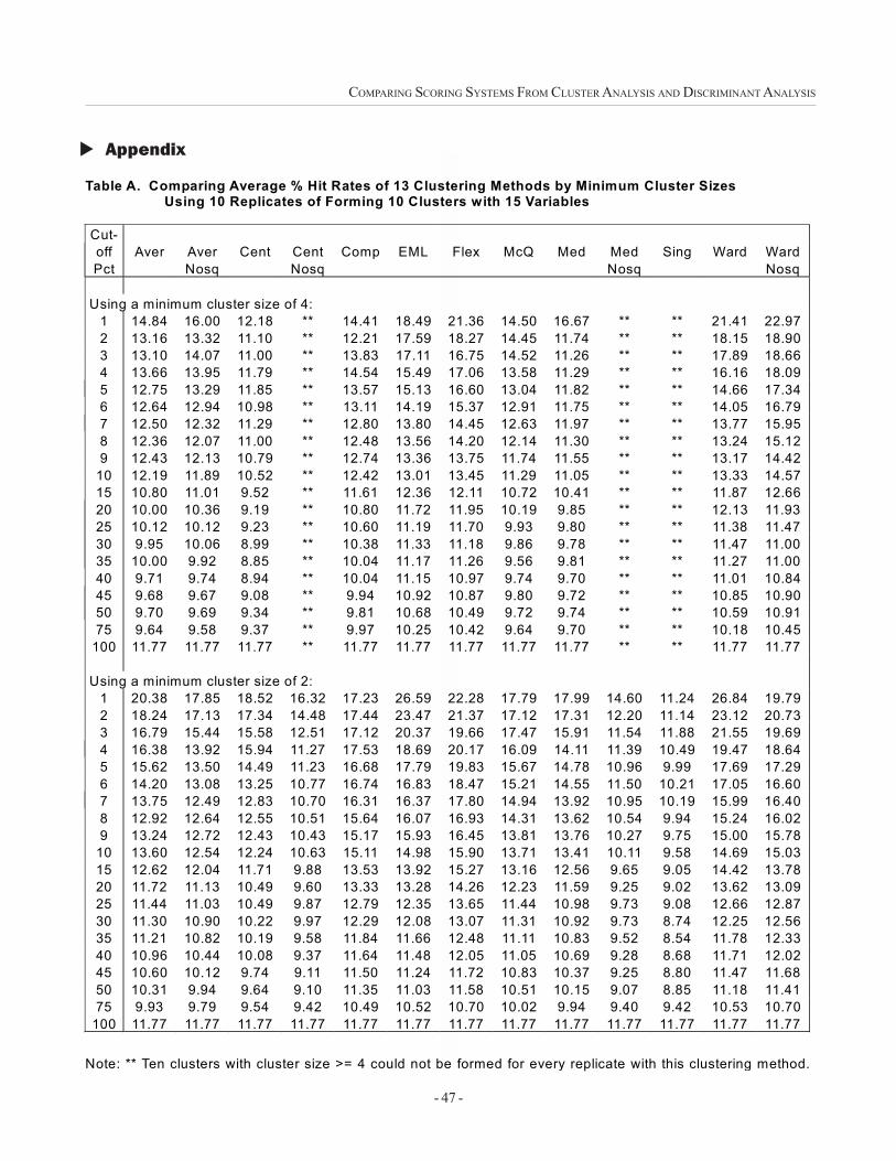
- 47 -
COMPARING SCORING SYSTEMS FROM CLUSTER ANALYSIS AND DISCRIMINANT ANALYSIS
� Appendix
Table A. Comparing Average % Hit Rates of 13 Clustering Methods by Minimum Cluster Sizes Using 10 Replicates of Forming 10 Clusters with 15 Variables
Cut- off Aver Aver Cent Cent Comp EML Flex McQ Med Med Sing Ward Ward Pct Nosq Nosq Nosq Nosq
Using a minimum cluster size of 4:
1 14.84 16.00 12.18 ** 14.41 18.49 21.36 14.50 16.67 ** ** 21.41 22.97 2 13.16 13.32 11.10 ** 12.21 17.59 18.27 14.45 11.74 ** ** 18.15 18.90 3 13.10 14.07 11.00 ** 13.83 17.11 16.75 14.52 11.26 ** ** 17.89 18.66 4 13.66 13.95 11.79 ** 14.54 15.49 17.06 13.58 11.29 ** ** 16.16 18.09 5 12.75 13.29 11.85 ** 13.57 15.13 16.60 13.04 11.82 ** ** 14.66 17.34 6 12.64 12.94 10.98 ** 13.11 14.19 15.37 12.91 11.75 ** ** 14.05 16.79 7 12.50 12.32 11.29 ** 12.80 13.80 14.45 12.63 11.97 ** ** 13.77 15.95 8 12.36 12.07 11.00 ** 12.48 13.56 14.20 12.14 11.30 ** ** 13.24 15.12 9 12.43 12.13 10.79 ** 12.74 13.36 13.75 11.74 11.55 ** ** 13.17 14.42
10 12.19 11.89 10.52 ** 12.42 13.01 13.45 11.29 11.05 ** ** 13.33 14.57 15 10.80 11.01 9.52 ** 11.61 12.36 12.11 10.72 10.41 ** ** 11.87 12.66 20 10.00 10.36 9.19 ** 10.80 11.72 11.95 10.19 9.85 ** ** 12.13 11.93 25 10.12 10.12 9.23 ** 10.60 11.19 11.70 9.93 9.80 ** ** 11.38 11.47 30 9.95 10.06 8.99 ** 10.38 11.33 11.18 9.86 9.78 ** ** 11.47 11.00 35 10.00 9.92 8.85 ** 10.04 11.17 11.26 9.56 9.81 ** ** 11.27 11.00 40 9.71 9.74 8.94 ** 10.04 11.15 10.97 9.74 9.70 ** ** 11.01 10.84 45 9.68 9.67 9.08 ** 9.94 10.92 10.87 9.80 9.72 ** ** 10.85 10.90 50 9.70 9.69 9.34 ** 9.81 10.68 10.49 9.72 9.74 ** ** 10.59 10.91 75 9.64 9.58 9.37 ** 9.97 10.25 10.42 9.64 9.70 ** ** 10.18 10.45
100 11.77 11.77 11.77 ** 11.77 11.77 11.77 11.77 11.77 ** ** 11.77 11.77 Using a minimum cluster size of 2:
1 20.38 17.85 18.52 16.32 17.23 26.59 22.28 17.79 17.99 14.60 11.24 26.84 19.79 2 18.24 17.13 17.34 14.48 17.44 23.47 21.37 17.12 17.31 12.20 11.14 23.12 20.73 3 16.79 15.44 15.58 12.51 17.12 20.37 19.66 17.47 15.91 11.54 11.88 21.55 19.69 4 16.38 13.92 15.94 11.27 17.53 18.69 20.17 16.09 14.11 11.39 10.49 19.47 18.64 5 15.62 13.50 14.49 11.23 16.68 17.79 19.83 15.67 14.78 10.96 9.99 17.69 17.29 6 14.20 13.08 13.25 10.77 16.74 16.83 18.47 15.21 14.55 11.50 10.21 17.05 16.60 7 13.75 12.49 12.83 10.70 16.31 16.37 17.80 14.94 13.92 10.95 10.19 15.99 16.40 8 12.92 12.64 12.55 10.51 15.64 16.07 16.93 14.31 13.62 10.54 9.94 15.24 16.02 9 13.24 12.72 12.43 10.43 15.17 15.93 16.45 13.81 13.76 10.27 9.75 15.00 15.78
10 13.60 12.54 12.24 10.63 15.11 14.98 15.90 13.71 13.41 10.11 9.58 14.69 15.03 15 12.62 12.04 11.71 9.88 13.53 13.92 15.27 13.16 12.56 9.65 9.05 14.42 13.78 20 11.72 11.13 10.49 9.60 13.33 13.28 14.26 12.23 11.59 9.25 9.02 13.62 13.09 25 11.44 11.03 10.49 9.87 12.79 12.35 13.65 11.44 10.98 9.73 9.08 12.66 12.87 30 11.30 10.90 10.22 9.97 12.29 12.08 13.07 11.31 10.92 9.73 8.74 12.25 12.56 35 11.21 10.82 10.19 9.58 11.84 11.66 12.48 11.11 10.83 9.52 8.54 11.78 12.33 40 10.96 10.44 10.08 9.37 11.64 11.48 12.05 11.05 10.69 9.28 8.68 11.71 12.02 45 10.60 10.12 9.74 9.11 11.50 11.24 11.72 10.83 10.37 9.25 8.80 11.47 11.68 50 10.31 9.94 9.64 9.10 11.35 11.03 11.58 10.51 10.15 9.07 8.85 11.18 11.41 75 9.93 9.79 9.54 9.42 10.49 10.52 10.70 10.02 9.94 9.40 9.42 10.53 10.70
100 11.77 11.77 11.77 11.77 11.77 11.77 11.77 11.77 11.77 11.77 11.77 11.77 11.77 Note: ** Ten clusters with cluster size >= 4 could not be formed for every replicate with this clustering method.
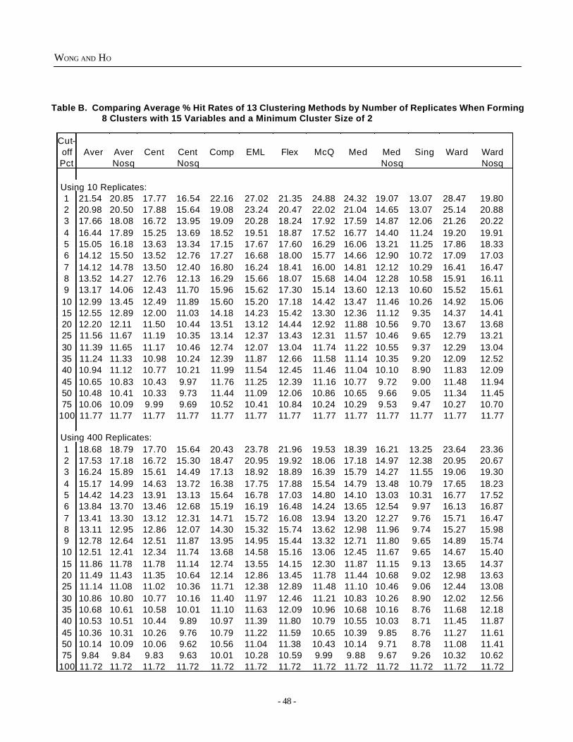
- 48 -
WONG AND HO
Table B. Comparing Average % Hit Rates of 13 Clustering Methods by Number of Replicates When Forming 8 Clusters with 15 Variables and a Minimum Cluster Size of 2
Cut- off Aver Aver Cent Cent Comp EML Flex McQ Med Med Sing Ward Ward Pct Nosq Nosq Nosq Nosq Using 10 Replicates:
1 21.54 20.85 17.77 16.54 22.16 27.02 21.35 24.88 24.32 19.07 13.07 28.47 19.80 2 20.98 20.50 17.88 15.64 19.08 23.24 20.47 22.02 21.04 14.65 13.07 25.14 20.88 3 17.66 18.08 16.72 13.95 19.09 20.28 18.24 17.92 17.59 14.87 12.06 21.26 20.22 4 16.44 17.89 15.25 13.69 18.52 19.51 18.87 17.52 16.77 14.40 11.24 19.20 19.91 5 15.05 16.18 13.63 13.34 17.15 17.67 17.60 16.29 16.06 13.21 11.25 17.86 18.33 6 14.12 15.50 13.52 12.76 17.27 16.68 18.00 15.77 14.66 12.90 10.72 17.09 17.03 7 14.12 14.78 13.50 12.40 16.80 16.24 18.41 16.00 14.81 12.12 10.29 16.41 16.47 8 13.52 14.27 12.76 12.13 16.29 15.66 18.07 15.68 14.04 12.28 10.58 15.91 16.11 9 13.17 14.06 12.43 11.70 15.96 15.62 17.30 15.14 13.60 12.13 10.60 15.52 15.61 10 12.99 13.45 12.49 11.89 15.60 15.20 17.18 14.42 13.47 11.46 10.26 14.92 15.06 15 12.55 12.89 12.00 11.03 14.18 14.23 15.42 13.30 12.36 11.12 9.35 14.37 14.41 20 12.20 12.11 11.50 10.44 13.51 13.12 14.44 12.92 11.88 10.56 9.70 13.67 13.68 25 11.56 11.67 11.19 10.35 13.14 12.37 13.43 12.31 11.57 10.46 9.65 12.79 13.21 30 11.39 11.65 11.17 10.46 12.74 12.07 13.04 11.74 11.22 10.55 9.37 12.29 13.04 35 11.24 11.33 10.98 10.24 12.39 11.87 12.66 11.58 11.14 10.35 9.20 12.09 12.52 40 10.94 11.12 10.77 10.21 11.99 11.54 12.45 11.46 11.04 10.10 8.90 11.83 12.09 45 10.65 10.83 10.43 9.97 11.76 11.25 12.39 11.16 10.77 9.72 9.00 11.48 11.94 50 10.48 10.41 10.33 9.73 11.44 11.09 12.06 10.86 10.65 9.66 9.05 11.34 11.45 75 10.06 10.09 9.99 9.69 10.52 10.41 10.84 10.24 10.29 9.53 9.47 10.27 10.70
100 11.77 11.77 11.77 11.77 11.77 11.77 11.77 11.77 11.77 11.77 11.77 11.77 11.77 Using 400 Replicates:
1 18.68 18.79 17.70 15.64 20.43 23.78 21.96 19.53 18.39 16.21 13.25 23.64 23.36 2 17.53 17.18 16.72 15.30 18.47 20.95 19.92 18.06 17.18 14.97 12.38 20.95 20.67 3 16.24 15.89 15.61 14.49 17.13 18.92 18.89 16.39 15.79 14.27 11.55 19.06 19.30 4 15.17 14.99 14.63 13.72 16.38 17.75 17.88 15.54 14.79 13.48 10.79 17.65 18.23 5 14.42 14.23 13.91 13.13 15.64 16.78 17.03 14.80 14.10 13.03 10.31 16.77 17.52 6 13.84 13.70 13.46 12.68 15.19 16.19 16.48 14.24 13.65 12.54 9.97 16.13 16.87 7 13.41 13.30 13.12 12.31 14.71 15.72 16.08 13.94 13.20 12.27 9.76 15.71 16.47 8 13.11 12.95 12.86 12.07 14.30 15.32 15.74 13.62 12.98 11.96 9.74 15.27 15.98 9 12.78 12.64 12.51 11.87 13.95 14.95 15.44 13.32 12.71 11.80 9.65 14.89 15.74 10 12.51 12.41 12.34 11.74 13.68 14.58 15.16 13.06 12.45 11.67 9.65 14.67 15.40 15 11.86 11.78 11.78 11.14 12.74 13.55 14.15 12.30 11.87 11.15 9.13 13.65 14.37 20 11.49 11.43 11.35 10.64 12.14 12.86 13.45 11.78 11.44 10.68 9.02 12.98 13.63 25 11.14 11.08 11.02 10.36 11.71 12.38 12.89 11.48 11.10 10.46 9.06 12.44 13.08 30 10.86 10.80 10.77 10.16 11.40 11.97 12.46 11.21 10.83 10.26 8.90 12.02 12.56 35 10.68 10.61 10.58 10.01 11.10 11.63 12.09 10.96 10.68 10.16 8.76 11.68 12.18 40 10.53 10.51 10.44 9.89 10.97 11.39 11.80 10.79 10.55 10.03 8.71 11.45 11.87 45 10.36 10.31 10.26 9.76 10.79 11.22 11.59 10.65 10.39 9.85 8.76 11.27 11.61 50 10.14 10.09 10.06 9.62 10.56 11.04 11.38 10.43 10.14 9.71 8.78 11.08 11.41 75 9.84 9.84 9.83 9.63 10.01 10.28 10.59 9.99 9.88 9.67 9.26 10.32 10.62
100 11.72 11.72 11.72 11.72 11.72 11.72 11.72 11.72 11.72 11.72 11.72 11.72 11.72
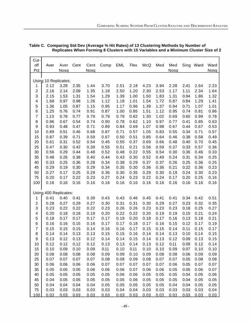
- 49 -
COMPARING SCORING SYSTEMS FROM CLUSTER ANALYSIS AND DISCRIMINANT ANALYSIS
Table C. Comparing Std Dev (Average % Hit Rates) of 13 Clustering Methods by Number of Replicates When Forming 8 Clusters with 15 Variables and a Minimum Cluster Size of 2
Cut- off Aver Aver Cent Cent Comp EML Flex McQ Med Med Sing Ward Ward Pct Nosq Nosq Nosq Nosq
Using 10 Replicates:
1 2.12 3.28 2.35 1.44 3.70 2.51 2.18 4.23 3.94 2.28 2.41 2.64 2.23 2 2.16 2.14 2.09 1.35 1.18 2.50 1.20 2.30 2.53 1.17 1.11 2.34 1.64 3 2.15 1.53 1.31 1.54 1.29 1.39 1.00 1.50 1.83 1.31 0.94 1.86 1.32 4 1.68 0.97 0.98 1.26 1.12 1.18 1.01 1.54 1.72 0.87 0.84 1.29 1.41 5 1.36 1.05 0.87 1.15 0.95 1.17 0.96 1.39 1.37 0.94 0.71 1.07 1.01 6 1.25 0.76 0.74 0.91 0.87 1.00 0.85 1.51 1.12 0.95 0.74 0.81 0.86 7 1.10 0.78 0.77 0.79 0.79 0.79 0.82 1.30 1.02 0.69 0.60 0.99 0.78 8 0.96 0.67 0.54 0.74 0.90 0.78 0.62 1.10 0.97 0.77 0.41 0.85 0.63 9 0.93 0.48 0.47 0.71 0.89 0.84 0.69 1.07 0.98 0.67 0.44 0.67 0.53
10 0.89 0.51 0.46 0.68 0.87 0.71 0.57 1.05 0.83 0.55 0.34 0.71 0.57 15 0.87 0.39 0.71 0.59 0.67 0.50 0.51 0.85 0.64 0.46 0.38 0.58 0.49 20 0.61 0.31 0.52 0.54 0.45 0.55 0.37 0.69 0.66 0.48 0.40 0.70 0.45 25 0.47 0.30 0.42 0.39 0.55 0.51 0.21 0.56 0.59 0.37 0.33 0.57 0.36 30 0.56 0.29 0.44 0.48 0.52 0.48 0.22 0.55 0.54 0.30 0.36 0.46 0.33 35 0.48 0.26 0.38 0.40 0.44 0.43 0.30 0.52 0.49 0.24 0.31 0.34 0.25 40 0.33 0.25 0.36 0.28 0.34 0.38 0.29 0.37 0.37 0.26 0.25 0.36 0.25 45 0.29 0.19 0.30 0.29 0.34 0.35 0.30 0.36 0.36 0.21 0.22 0.36 0.23 50 0.27 0.17 0.25 0.29 0.36 0.30 0.35 0.29 0.30 0.19 0.24 0.30 0.23 75 0.20 0.17 0.22 0.23 0.27 0.24 0.23 0.22 0.24 0.17 0.20 0.25 0.16
100 0.16 0.16 0.16 0.16 0.16 0.16 0.16 0.16 0.16 0.16 0.16 0.16 0.16 Using 400 Replicates:
1 0.41 0.40 0.41 0.39 0.43 0.43 0.46 0.45 0.41 0.41 0.34 0.42 0.51 2 0.28 0.27 0.29 0.27 0.30 0.31 0.31 0.30 0.29 0.27 0.23 0.32 0.35 3 0.23 0.22 0.22 0.22 0.23 0.26 0.26 0.23 0.23 0.23 0.18 0.25 0.27 4 0.20 0.18 0.18 0.19 0.20 0.22 0.22 0.20 0.19 0.19 0.15 0.21 0.24 5 0.18 0.17 0.17 0.17 0.17 0.19 0.20 0.18 0.17 0.16 0.13 0.18 0.21 6 0.16 0.16 0.15 0.16 0.17 0.17 0.18 0.17 0.16 0.15 0.12 0.17 0.19 7 0.15 0.15 0.15 0.14 0.16 0.16 0.17 0.15 0.15 0.14 0.11 0.15 0.17 8 0.14 0.14 0.13 0.13 0.15 0.15 0.16 0.14 0.14 0.13 0.10 0.14 0.15 9 0.13 0.12 0.13 0.12 0.14 0.14 0.15 0.14 0.13 0.12 0.09 0.13 0.15
10 0.12 0.12 0.12 0.12 0.13 0.13 0.14 0.13 0.12 0.11 0.09 0.12 0.14 15 0.10 0.09 0.10 0.09 0.11 0.10 0.11 0.10 0.10 0.09 0.07 0.10 0.10 20 0.08 0.08 0.08 0.08 0.09 0.09 0.10 0.09 0.08 0.08 0.06 0.09 0.09 25 0.07 0.07 0.07 0.07 0.08 0.08 0.09 0.08 0.07 0.07 0.05 0.08 0.08 30 0.06 0.06 0.06 0.06 0.07 0.07 0.07 0.07 0.07 0.06 0.05 0.07 0.07 35 0.05 0.05 0.05 0.06 0.06 0.06 0.07 0.06 0.06 0.05 0.05 0.06 0.07 40 0.05 0.05 0.05 0.05 0.05 0.06 0.06 0.05 0.05 0.05 0.04 0.05 0.06 45 0.04 0.05 0.05 0.05 0.05 0.05 0.06 0.05 0.05 0.05 0.04 0.05 0.05 50 0.04 0.04 0.04 0.04 0.05 0.05 0.05 0.05 0.05 0.04 0.04 0.05 0.05 75 0.03 0.03 0.03 0.03 0.03 0.04 0.04 0.03 0.03 0.03 0.03 0.03 0.04
100 0.03 0.03 0.03 0.03 0.03 0.03 0.03 0.03 0.03 0.03 0.03 0.03 0.03
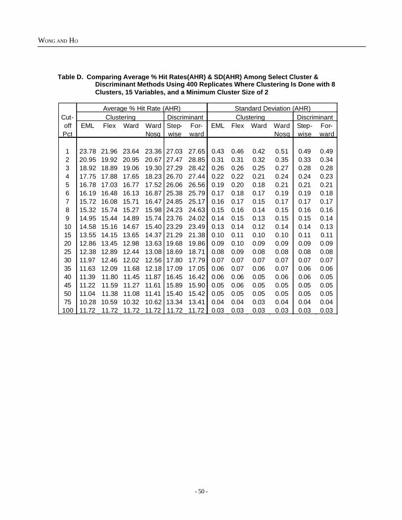
- 50 -
WONG AND HO
Table D. Comparing Average % Hit Rates(AHR) & SD(AHR) Among Select Cluster & Discriminant Methods Using 400 Replicates Where Clustering Is Done with 8 Clusters, 15 Variables, and a Minimum Cluster Size of 2
Average % Hit Rate (AHR) Standard Deviation (AHR) Cut- Clustering Discriminant Clustering Discriminant off EML Flex Ward Ward Step- For- EML Flex Ward Ward Step- For- Pct Nosq wise ward Nosq wise ward
1 23.78 21.96 23.64 23.36 27.03 27.65 0.43 0.46 0.42 0.51 0.49 0.49 2 20.95 19.92 20.95 20.67 27.47 28.85 0.31 0.31 0.32 0.35 0.33 0.34 3 18.92 18.89 19.06 19.30 27.29 28.42 0.26 0.26 0.25 0.27 0.28 0.28 4 17.75 17.88 17.65 18.23 26.70 27.44 0.22 0.22 0.21 0.24 0.24 0.23 5 16.78 17.03 16.77 17.52 26.06 26.56 0.19 0.20 0.18 0.21 0.21 0.21 6 16.19 16.48 16.13 16.87 25.38 25.79 0.17 0.18 0.17 0.19 0.19 0.18 7 15.72 16.08 15.71 16.47 24.85 25.17 0.16 0.17 0.15 0.17 0.17 0.17 8 15.32 15.74 15.27 15.98 24.23 24.63 0.15 0.16 0.14 0.15 0.16 0.16 9 14.95 15.44 14.89 15.74 23.76 24.02 0.14 0.15 0.13 0.15 0.15 0.14 10 14.58 15.16 14.67 15.40 23.29 23.49 0.13 0.14 0.12 0.14 0.14 0.13 15 13.55 14.15 13.65 14.37 21.29 21.38 0.10 0.11 0.10 0.10 0.11 0.11 20 12.86 13.45 12.98 13.63 19.68 19.86 0.09 0.10 0.09 0.09 0.09 0.09 25 12.38 12.89 12.44 13.08 18.69 18.71 0.08 0.09 0.08 0.08 0.08 0.08 30 11.97 12.46 12.02 12.56 17.80 17.79 0.07 0.07 0.07 0.07 0.07 0.07 35 11.63 12.09 11.68 12.18 17.09 17.05 0.06 0.07 0.06 0.07 0.06 0.06 40 11.39 11.80 11.45 11.87 16.45 16.42 0.06 0.06 0.05 0.06 0.06 0.05 45 11.22 11.59 11.27 11.61 15.89 15.90 0.05 0.06 0.05 0.05 0.05 0.05 50 11.04 11.38 11.08 11.41 15.40 15.42 0.05 0.05 0.05 0.05 0.05 0.05 75 10.28 10.59 10.32 10.62 13.34 13.41 0.04 0.04 0.03 0.04 0.04 0.04
100 11.72 11.72 11.72 11.72 11.72 11.72 0.03 0.03 0.03 0.03 0.03 0.03
�
3
New Developments in TaxStatistics and Administrative
Records
Sailer Gurka HoldenLegel Bennett Parisi
Kilss JordanDixon
Petska Kilss
� �
� �
�
�
- 53 -
Accumulation and Distributions of Retirement Assets,1996-2000: Results From a Matched File of Tax Returns
and Information ReturnsPeter Sailer and Kurt S. Gurka, Internal Revenue Service,
and Sarah Holden, Investment Company Institute
D eductions for contributions to Individual Retire-ment Arrangements (IRA’s) appeared on Form1040 for the first time for Tax Year 1975, and
the 1975 version of the annual report, Statistics ofIncome—Individual Income Tax Returns, duly re-corded the number of returns with an entry on that line—1.2 million—and the amount deducted—about $1.4 bil-lion (Figure 1). Twenty-five years and many tax lawchanges later, the 2000 Individual Income Tax Returnsreport still tabulated the entries on this line, amountingto 3.5 million returns and $7.5 billion in deductible tradi-tional IRA contributions.
However important these statistics have been to theanalysis of IRA’s over the years, they have not told thefull story. For example, during Tax Year 2000, in addi-tion to the $7.5 billion in tax-deductible contributions totraditional IRA plans, $2.5 billion in nondeductible con-tributions were also made to such plans (Figure 2). Fur-thermore, other types of IRA received $26.3 billion incontributions. However, much more importantly, $225.6billion of assets were rolled over into IRA’s from otherqualified pension plans and tax-sheltered annuities. Thesethree statistics were taken from Forms 5498 filed withthe Internal Revenue Service by IRA trustees.1 Form5498 also shows the total fair market value (FMV) ofassets held in IRA’s. At the end of Tax Year 2000, thetotal value of IRA assets stood at $2.6 trillion.
In the following paper, the authors use never-be-fore-released IRS data1 from Form 5498, along withhousehold survey and other information, to highlight keydemographic and financial characteristics of traditionalIRA owners and their traditional IRA assets. Historicaltrends will be noted. In addition, again using the matchedfile of tax returns and Forms W-2, some summary sta-tistics on 401(k) plans are presented.
u Assets Held in IRA’s
Types of IRAs. The predominant type of IRA isthe traditional IRA, which was created with the Em-
ployee Retirement Income Security Act (ERISA) of1974. Indeed, SOI estimates indicate that about 92 per-cent of all IRA assets were held in traditional IRA’s atyearend 2000 (Figure 2). Roth IRA’s (created in theTaxpayer Relief Act of 1997) represented about 3 per-cent of all IRA assets, while employer-sponsored IRA’s(SEP IRA’s—created in the Revenue Act of 1978, SAR-SEP IRA’s—created in the Tax Reform Act of 1986,and SIMPLE IRA’s—created in the Small Business JobProtection Act of 1996) held about 6 percent of the to-tal. Education IRA’s (created in the Taxpayer ReliefAct of 1997), which are now known as Coverdell Edu-cation Savings Accounts (ESA’s), accounted for a neg-ligible share of the total.2
Types of Assets. Figure 3, based in part on IRSstatistics and in part on surveys by the Investment Com-pany Institute (ICI), shows that at yearend 2002, IRAassets amounted to an estimated $2.3 trillion, comparedwith $637 billion at yearend 1990. With more than halfof IRA assets invested in equity securities, the effect ofthe stock market can also be seen in recent years. In-deed, IRA assets reached nearly $2.7 trillion at year-end 1999 during the bull market in equities, then begandeclining. IRA assets are invested in a variety of finan-cial institutions. At yearend 2002, about 46 percent ofall IRA assets were invested in mutual funds, another 34percent were in non-mutual fund securities held throughbrokerage accounts, another 11 percent were held in bankand thrift deposits, and the remaining 9 percent wereheld in annuities at life insurance companies.3
u Demographic Composition and IRABalances of Traditional IRA Owners
Data from Tax Returns and InformationReturns
Age Distribution, by Taxpayer. The SOI data,which are based on a weighted sample of tax-return in-formation,4 allow analysis of IRA-owning taxpayers atyearend 1999 by age, marital status on the tax return,
- 54 -
SAILER, GURKA, AND HOLDEN
gender, and income. Traditional IRA owners are pre-dominantly middle-aged. Twenty percent of the 36.6million taxpayers with traditional IRA’s in 1999 were 35to 44 years of age, and another 25 percent were age 45to 54 (Figure 4). About 14 percent of taxpayers owningIRA’s in 1999 were age 70 or older, which places themin the age group that must take required minimum distri-butions from their accounts.
Marital Status and Gender, by Taxpayer. Themajority of traditional IRA-owning taxpayers are mar-ried filing joint returns, and half of traditional IRA- own-ing taxpayers are male. Among the 36.6 million tradi-tional IRA-owning taxpayers at yearend 1999, nearlythree-quarters were married (Figure 5).5 Half of tradi-tional IRA-owning taxpayers were married with bothspouses holding traditional IRA’s. Single women ac-counted for 16 percent of traditional IRA-owning tax-payers, and single men accounted for 10 percent.
Traditional IRA Balances, by Age of Taxpayer.There is a wide range of traditional IRA balances heldby taxpayers around an average of $66,179 at yearend1999.6 Because older taxpayers have had more time towork and accumulate IRA assets, either from rolloverat job change or from contributions over time, older tax-payers tend to have higher traditional IRA balances. Theaverage traditional IRA balance held by taxpayers 25 to34 years old was $12,435 at yearend 1999, while theaverage balance peaks among taxpayers aged 65 to 69at $112,588, even though they may take distributionswithout penalty (Figure 4). Among taxpayers aged 70and older, the average traditional IRA balance falls, per-haps because those individuals are taking withdrawalsto fund retirement at least at the level of the requiredminimum distribution.
Traditional IRA Balances, by Marital Status andGender of Taxpayer. There is a wide range of aver-age traditional IRA balances by marital status and gen-der among taxpayers analyzed in the SOI data. Althoughit is difficult to interpret the significance of average ac-count balances for a snapshot of one period in time, it isinteresting to note that single taxpayers have similar av-erage account balances regardless of gender (Figure 5).On the other hand, among married taxpayers, the hus-bands’ average IRA assets were higher than the wives.’
The traditional IRA assets at yearend 1999 represent anaccumulation of activity starting possibly as far back as1974 (when traditional IRAs were created). The loweraverage among wives may be driven by women’s typi-cally discontinuous work histories and therefore lowerrollover amounts available to go into an IRA.7 In addi-tion, regulations restricting tax-deductible spousal con-tributions may also have damped wives’ IRA assets. Togain a better understanding of the differential in averageIRA assets between husbands and wives, data for thesame individuals would need to be tracked for severalyears—monitoring contributions, rollovers, andworkforce participation (and pension coverage therein).Unfortunately, such insight, while planned, will not beavailable for several years.
u Traditional IRA's: Comparison of SOIData and Household SurveyInformation
Although it is difficult to match up household andtaxpayer information,8 this section makes some broadcomparisons between the SOI data and household sur-veys conducted by ICI and the Federal Reserve Board.The IRS SOI tax return and information return data,which are based on a weighted sample of returns, findsimilar demographic characteristics for the typical (me-dian) traditional IRA owner as these household surveysfind. Furthermore, similar to household survey informa-tion, the median traditional IRA balance among tax re-turns with traditional IRA owners was $27,181 at yearend1999 (Figure 6).
Age and Marital Status of Typical TraditionalIRA Owner. The typical traditional IRA owner is about50 years old. For example, ICI’s June 1999 survey findsa median age among traditional IRA-owning householdsof 49 years, and ICI’s June 2000 survey finds a medianage of 53 years (Figure 6). Similarly, ICI tabulations9 ofthe Federal Reserve Board’s Survey of Consumer Fi-nances (SCF) data indicate that the median age of IRA-owning households was 51 in both the 1998 and 2001surveys. Likewise, the median taxpayer owning traditionalIRA’s in the SOI data was 53 years old in 1999. Thetypical traditional IRA owner is married. In the house-hold surveys and the SOI tax return data, about two-thirds of households with traditional IRA’s are married.
- 55 -
ACCUMULATION AND DISTRIBUTIONS OF RETIREMENT ASSETS, 1996-2000
u Demographic Composition andContribution Activity of 401(k)Participants
SOI Data Based on IRS Tax Returns andInformation Returns
Although Section 401(k) of the Internal RevenueCode was created in the Revenue Act of 1978, clarifi-cation of the regulations did not occur until 1981. Afterthat slow start, 401(k) plans have grown rapidly through-out the 1990’s. At yearend 2002—401(k) plans held$1.54 trillion in assets (Figure 7). The key provision of401(k) plans is the ability to defer salary by making be-fore-tax contributions (deferrals) to an account main-tained in the given participant’s name. In most instances,the participant directs the investment of the account as-sets, which grow tax-free until they are withdrawn. Inmany cases, the plan sponsor may make a matchingcontribution (for example, contributing 50 cents for ev-ery dollar the participant contributes up to 6 percent ofsalary).10 Contributions-by-plan participants depend ona variety of factors, including the regulatory frameworkunder which 401(k) plans operate, personal participantcharacteristics, and plan design features.11 Using IRSW-2 form information, a glimpse at elective deferrals bytaxpayers into 401(k) plans is possible.
401(k) Elective Deferrals . W-2 Form informa-tion indicates that elective deferrals by 401(k) plan par-ticipants rose steadily from 1996 through 2002, from $61billion to nearly $105 billion (Figure 7).12 In addition, thenumber of taxpayers with deferrals and the averagedeferral amount also increased over the late 1990’s.Indeed, average deferrals rose from $2,660 in 1996 to$3,408 in 2000.
Age of 401(k) Participants. The average andmedian age of taxpayer with 401(k) elective deferralswas 42 in 1999.13 The bulk of deferrals in 1999 weremade by taxpayers in their thirties, forties, or fifties.Average deferrals tend to rise with age through the agegroup in their fifties, and decline a bit among taxpayersin their sixties and older.
u Conclusions and Future Research
With nearly $4.0 trillion invested in IRA’s and 401(k)plans at yearend 2003, these retirement savings vehiclesrepresent a significant component of Americans’ finan-cial security. Taxpayers holding IRAs and 401(k) ac-counts cover a wide range of ages and incomes. Thispaper provided a glimpse at the rich detail available fromthe SOI sample of tax returns and information returns(focusing in detail on 1999). The results of this analysisof SOI data are encouraging. The typical IRA- owningtaxpayer represented in the SOI data appears to be simi-lar in basic demographic and financial characteristics tothe typical IRA-owning household found in householdsurveys conducted by ICI and the Federal ReserveBoard. The SOI 401(k) participant information in ag-gregate corresponds well to Form 5500 results, and thepreliminary age analysis is similar to EBRI/ICI results.
Future research would extend both the IRA and401(k) detailed analyses to more years. In addition, fu-ture data would analyze the taxpayers by type of IRA.Furthermore, longitudinal analysis tracking the behav-iors of IRA owners and 401(k) participants over timeshould also be explored.
u Acknowledgment
The authors would like to extend their thanks toMarianne Cooley of the IRS Computing Center in De-troit, Michigan, for many years of stewardship of theSOI Information Returns data base.
u References
Federal Reserve Board. Survey of ConsumerFinances. Available at: http://www.federalreserve.gov/pubs/oss/oss2/scfindex.html
Holden, Sarah and VanDerhei, Jack, “ContributionBehavior of 401(k) Plan Participants.” ICI Per-spective, Vol. 7, No. 4, and EBRI Issue Brief, No.238. Washington, DC, Investment CompanyInstitute and Employee Benefit Research Institute,October 2001.
- 56 -
SAILER, GURKA, AND HOLDEN
Holden, Sarah and VanDerhei, Jack, “401(k) PlanAsset Allocation, Account Balances, and LoanActivity in 1999,” ICI Perspective, Vol. 7, No. 1,and EBRI Issue Brief, No. 230, Washington, DC,Investment Company Institute, January 2001,and Employee Benefit Research Institute, Febru-ary 2001.
Investment Company Institute, “IRA Ownership in2003,” Fundamentals, Vol. 12, No. 3, Washington,DC, Investment Company Institute, September 2003.
———, “Mutual Funds and the U.S. RetirementMarket in 2002,” ICI Fundamentals, Vol. 12, No.1, Washington, DC, Investment Company Institute,June 2003.
———, “IRA Ownership in 2002,” Fundamentals,Vol. 11, No. 3, Washington, DC, InvestmentCompany Institute, September 2002.
———, “IRA Ownership in 2001,” Fundamentals,Vol. 10, No. 3, Washington, DC, InvestmentCompany Institute, September 2001.
———, “IRA Ownership in 2000,” Fundamentals,Vol. 9, No. 5, Washington, DC, Investment Com-pany Institute, October 2000.
———, “IRA Ownership in 1999,” Fundamentals,Vol. 8, No. 6, Washington, DC, Investment Com-pany Institute, December 1999.
Sailer, Peter J.; Weber, Michael E.; Gurka, Kurt S.,“Are Taxpayers Increasing the Buildup of Retire-ment Assets? Preliminary Results from a MatchedFile of Tax Year 1999 Tax Returns and Informa-tion Returns,” paper presented at National TaxAssociation 95th Annual Conference in Orlando,FL, November 15, 2002.
U.S. Department of Labor, Employee Benefits Secu-rity Administration, “Women and RetirementSavings.” Available at: http://www.dol.gov/ebsa/publications/women.html
U.S. Internal Revenue Service, Publication 590Individual Retirement Arrangements (IRA’s).
Washington, DC, U.S. Department of the Trea-sury, Internal Revenue Service, 1999 and 2002.Available at: www.irs.gov/pub/irs-99/p590.pdf(1999) and www.irs.gov/pub/irs-pdf/p590.pdf
U.S. Internal Revenue Service, Statistics of Income,2000 Individual Income Tax Returns, Washing-ton, DC, March 2003.
U.S. Internal Revenue Service, Statistics of Income,1975 Individual Income Tax Returns, Washing-ton, DC, 1978.
U.S. Internal Revenue Service, Statistics of Income,Individual Income Tax Returns, Publication1304, Washington, DC, various years.
u Footnotes
1 All SOI data are based on a stratified weightedsample of individual income tax returns with match-ing information returns. See Sailer, Weber, andGurka (November 2002) for SOI data estima-tion methodology.
2 The estimate for education IRA’s, or CoverdellESA’s, is underestimated in Figure 2, as nonfilingdependents are not included in the estimation.
3 Figure 3 reports aggregate IRA assets; it does notindicate what individual IRA owners may be hold-ing. An ICI survey of IRA owning households inmid-2003 reports the incidence of the different typesof financial assets held in IRA’s (see InvestmentCompany Institute (September 2003)).
4 See text footnote 1.
5 A small number of married-filing-separate returnsare included as single. Some of these taxpayersare in fact in the middle of separation or divorceproceedings and are not, in fact, living together.
6 Among the 36.6 million taxpayers with traditionalIRAs at yearend 1999, some 20.6 percent had tra-ditional IRA balances of less than $5,000; 28.6 per-cent had traditional IRA balances between $5,000and $20,000; 17.8 percent had balances between
- 57 -
ACCUMULATION AND DISTRIBUTIONS OF RETIREMENT ASSETS, 1996-2000
$20,000 and $40,000; 18.7 percent had balancesbetween $40,000 and $100,000; and 14.3 percenthad traditional IRA balances of $100,000 or more.
7 The U.S. Department of Labor’s “Women and Re-tirement Savings” notes that women are more likelyto work in part-time jobs that do not qualify for pen-sion coverage or to have lapses in pension cover-age because of interruptions in their careers to takecare of family members.
8 Exact comparison is not possible for several rea-sons including: (1) not all households file tax re-turns, (2) household units do not always correspondto tax return units, for example, a household withunmarried partners will appear as one household ina household survey, but as two single tax returns,(3) household surveys rely on self-reported infor-mation, which can suffer from participant recall,while the tax return information is unaudited taxreturn information, which may contain reportingerrors, (4) the definition of income may vary acrossdata sources, and (5) the timing of the surveys/re-turns varies.
9 Special thanks to Michael Bogdan at ICI for tabu-lating the SCF data.
10 See Investment Company Institute (June 2003).
11 For a comprehensive study of 401(k) participantcontribution activity, see Holden and VanDerhei(October 2001).
12 The new tabulations from Forms W-2 produce simi-lar estimates for aggregate deferrals as U.S. De-partment of Labor tabulations of employee contri-butions from Forms 5500 (Figure 7).
13 About 13 percent of these taxpayers were in theirtwenties; 30 percent were in their thirties; 31 per-cent were in their forties; 20 percent were in theirfifties; and 5 percent were in their sixties. This agedistribution is essentially the same as the age distri-bution of active 401(k) plan participants in the col-laborative data base maintained by the EmployeeBenefit Research Institute (EBRI) and ICI, knownas the EBRI/ICI Participant-Directed RetirementPlan Data Collection Project (see Holden andVanDerhei (January/February 2001)).
u Note
The views in this paper are those of the authors anddo not reflect those of the Investment Company Insti-tute or its members, nor are they the official positions ofthe Internal Revenue Service. Any errors are solely theresponsibility of the authors.
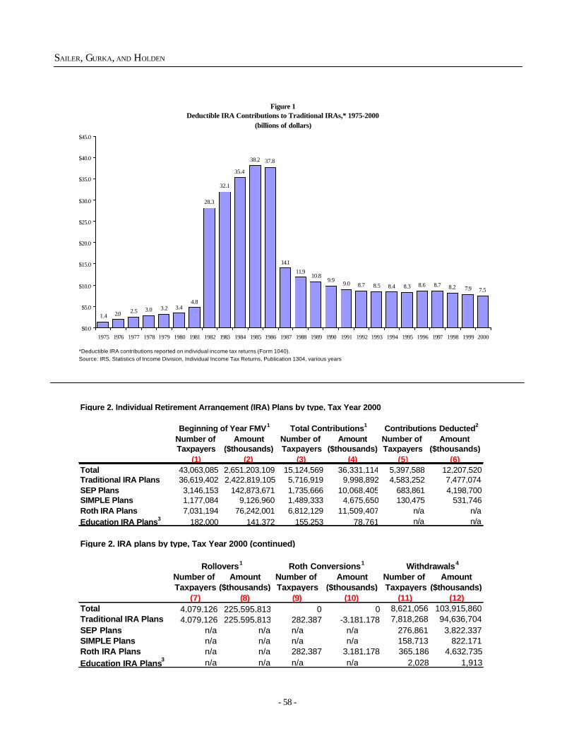
- 58 -
SAILER, GURKA, AND HOLDEN
Figure 1 Deductible IRA Contributions to Traditional IRAs,* 1975-2000
(billions of dollars)
1.4 2.0 2.5 3.0 3.2 3.44.8
28.3
32.1
35.4
38.2 37.8
14.1
11.910.8
9.9 9.0 8.7 8.5 8.4 8.3 8.6 8.7 8.2 7.9 7.5
$0.0
$5.0
$10.0
$15.0
$20.0
$25.0
$30.0
$35.0
$40.0
$45.0
1975 1976 1977 1978 1979 1980 1981 1982 1983 1984 1985 1986 1987 1988 1989 1990 1991 1992 1993 1994 1995 1996 1997 1998 1999 2000
*Deductible IRA contributions reported on individual income tax returns (Form 1040).Source: IRS, Statistics of Income Division, Individual Income Tax Returns, Publication 1304, various years
Figure 2. Individual Retirement Arrangement (IRA) Plans by type, Tax Year 2000
Number of Amount Number of Amount Number of AmountTaxpayers ($thousands) Taxpayers ($thousands) Taxpayers ($thousands)
(1) (2) (3) (4) (5) (6)Total 43,063,085 2,651,203,109 15,124,569 36,331,114 5,397,588 12,207,520Traditional IRA Plans 36,619,402 2,422,819,105 5,716,919 9,998,892 4,583,252 7,477,074SEP Plans 3,146,153 142,873,671 1,735,666 10,068,405 683,861 4,198,700SIMPLE Plans 1,177,084 9,126,960 1,489,333 4,675,650 130,475 531,746Roth IRA Plans 7,031,194 76,242,001 6,812,129 11,509,407 n/a n/aEducation IRA Plans3 182,000 141,372 155,253 78,761 n/a n/a
Beginning of Year FMV1 Total Contributions1 Contributions Deducted2
Figure 2. IRA plans by type, Tax Year 2000 (continued)
Number of Amount Number of Amount Number of AmountTaxpayers ($thousands) Taxpayers ($thousands) Taxpayers ($thousands)
(7) (8) (9) (10) (11) (12)Total 4,079,126 225,595,813 0 0 8,621,056 103,915,860Traditional IRA Plans 4,079,126 225,595,813 282,387 -3,181,178 7,818,268 94,636,704SEP Plans n/a n/a n/a n/a 276,861 3,822,337SIMPLE Plans n/a n/a n/a n/a 158,713 822,171Roth IRA Plans n/a n/a 282,387 3,181,178 365,186 4,632,735Education IRA Plans3 n/a n/a n/a n/a 2,028 1,913
Roth Conversions1 Withdrawals4Rollovers1
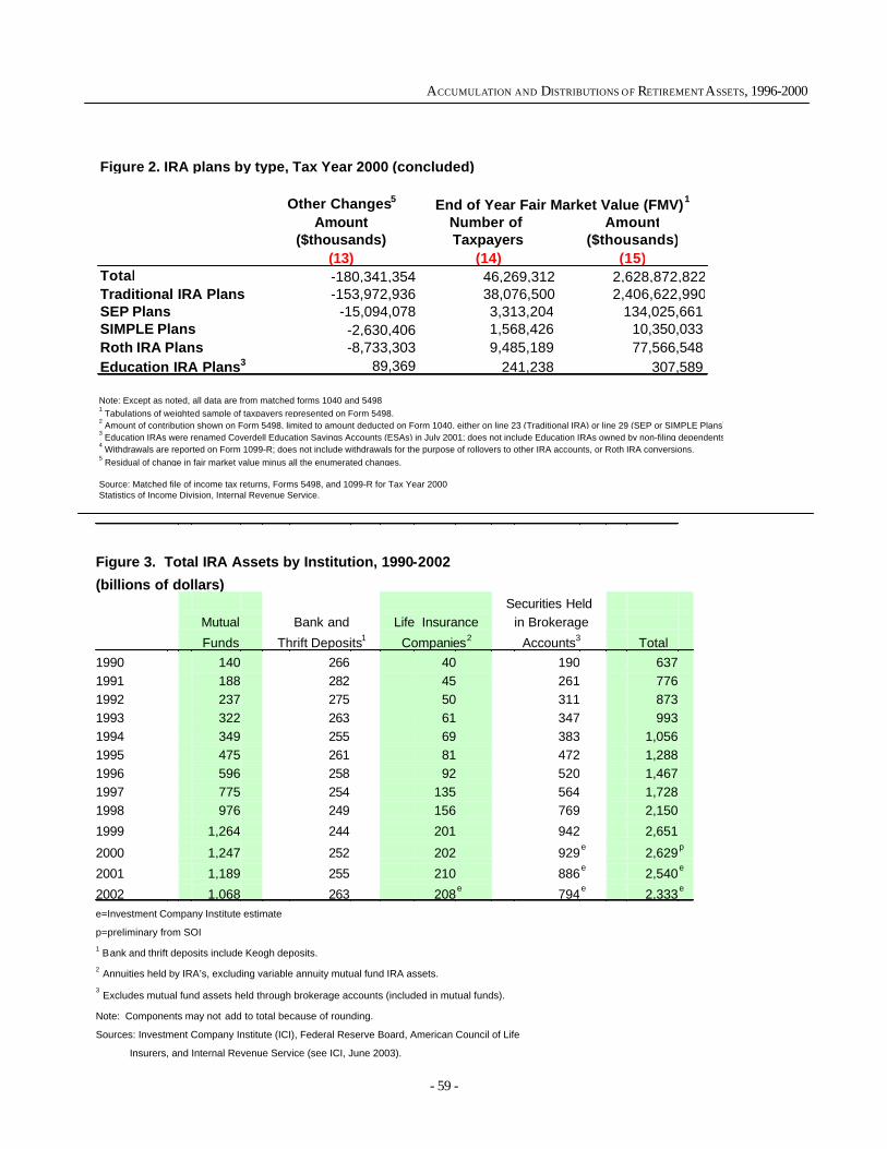
- 59 -
ACCUMULATION AND DISTRIBUTIONS OF RETIREMENT ASSETS, 1996-2000
Figure 2. IRA plans by type, Tax Year 2000 (concluded)
Other Changes5
Amount Number of Amount($thousands) Taxpayers ($thousands)
(13) (14) (15)Total -180,341,354 46,269,312 2,628,872,822Traditional IRA Plans -153,972,936 38,076,500 2,406,622,990SEP Plans -15,094,078 3,313,204 134,025,661SIMPLE Plans -2,630,406 1,568,426 10,350,033Roth IRA Plans -8,733,303 9,485,189 77,566,548Education IRA Plans3 89,369 241,238 307,589
End of Year Fair Market Value (FMV)1
Note: Except as noted, all data are from matched forms 1040 and 54981 Tabulations of weighted sample of taxpayers represented on Form 5498.
2 Amount of contribution shown on Form 5498, limited to amount deducted on Form 1040, either on line 23 (Traditional IRA) or line 29 (SEP or SIMPLE Plans).
3 Education IRAs were renamed Coverdell Education Savings Accounts (ESAs) in July 2001; does not include Education IRAs owned by non-filing dependents.
4 Withdrawals are reported on Form 1099-R; does not include withdrawals for the purpose of rollovers to other IRA accounts, or Roth IRA conversions.
5 Residual of change in fair market value minus all the enumerated changes.
Source: Matched file of income tax returns, Forms 5498, and 1099-R for Tax Year 2000Statistics of Income Division, Internal Revenue Service.
Figure 3. Total IRA Assets by Institution, 1990-2002
(billions of dollars) Securities Held Mutual Bank and Life Insurance in Brokerage
Funds Thrift Deposits1 Companies2 Accounts3 Total 1990 140 266 40 190 637 1991 188 282 45 261 776 1992 237 275 50 311 873 1993 322 263 61 347 993 1994 349 255 69 383 1,056 1995 475 261 81 472 1,288 1996 596 258 92 520 1,467 1997 775 254 135 564 1,728 1998 976 249 156 769 2,150
1999 1,264 244 201 942 2,651
2000 1,247 252 202 929 e 2,629 p
2001 1,189 255 210 886 e 2,540 e
2002 1,068 263 208 e 794 e 2,333 e e=Investment Company Institute estimate p=preliminary from SOI 1 Bank and thrift deposits include Keogh deposits. 2 Annuities held by IRA’s, excluding variable annuity mutual fund IRA assets. 3 Excludes mutual fund assets held through brokerage accounts (included in mutual funds).
Note: Components may not add to total because of rounding. Sources: Investment Company Institute (ICI), Federal Reserve Board, American Council of Life
Insurers, and Internal Revenue Service (see ICI, June 2003).
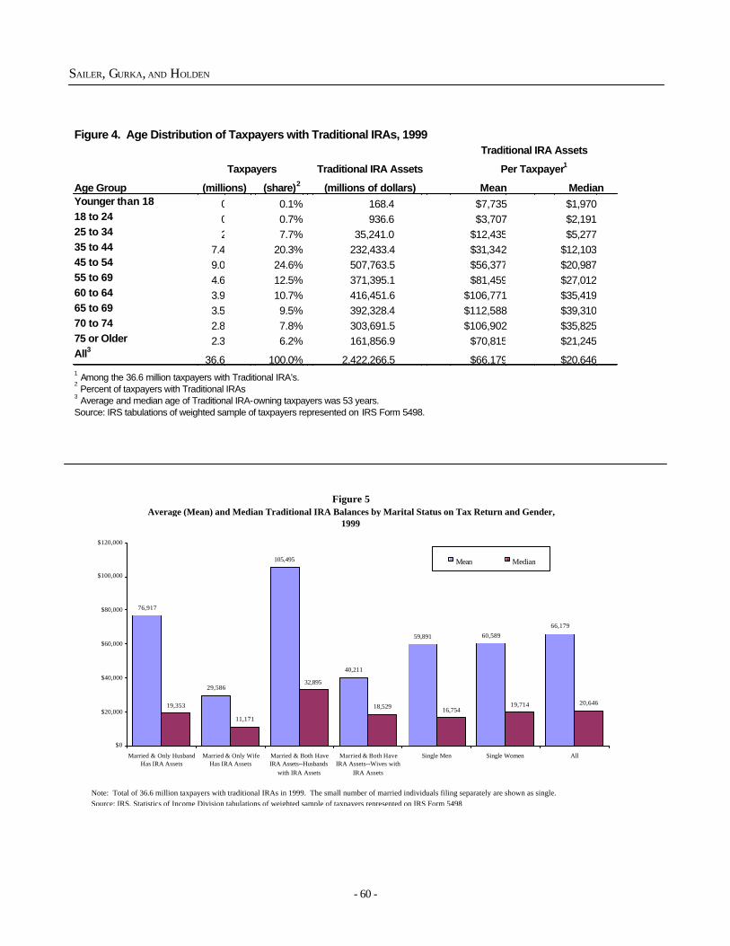
- 60 -
SAILER, GURKA, AND HOLDEN
Figure 4. Age Distribution of Taxpayers with Traditional IRAs, 1999 Traditional IRA Assets
Taxpayers Traditional IRA Assets Per Taxpayer1
Age Group (millions) (share)2 (millions of dollars) Mean Median Younger than 18 0.0 0.1% 168.4 $7,735 $1,970 18 to 24 0.3 0.7% 936.6 $3,707 $2,191 25 to 34 2.8 7.7% 35,241.0 $12,435 $5,277 35 to 44 7.4 20.3% 232,433.4 $31,342 $12,103 45 to 54 9.0 24.6% 507,763.5 $56,377 $20,987 55 to 69 4.6 12.5% 371,395.1 $81,459 $27,012 60 to 64 3.9 10.7% 416,451.6 $106,771 $35,419 65 to 69 3.5 9.5% 392,328.4 $112,588 $39,310 70 to 74 2.8 7.8% 303,691.5 $106,902 $35,825 75 or Older 2.3 6.2% 161,856.9 $70,815 $21,245 All3 36.6 100.0% 2,422,266.5 $66,179 $20,646
1 Among the 36.6 million taxpayers with Traditional IRA’s. 2 Percent of taxpayers with Traditional IRAs
3 Average and median age of Traditional IRA-owning taxpayers was 53 years. Source: IRS tabulations of weighted sample of taxpayers represented on IRS Form 5498.
Figure 5Average (Mean) and Median Traditional IRA Balances by Marital Status on Tax Return and Gender,
1999
76,917
29,586
105,495
40,211
59,891 60,589
66,179
19,353
11,171
32,895
18,529 16,75419,714 20,646
$0
$20,000
$40,000
$60,000
$80,000
$100,000
$120,000
Married & Only HusbandHas IRA Assets
Married & Only WifeHas IRA Assets
Married & Both HaveIRA Assets--Husbands
with IRA Assets
Married & Both HaveIRA Assets--Wives with
IRA Assets
Single Men Single Women All
Mean Median
Note: Total of 36.6 million taxpayers with traditional IRAs in 1999. The small number of married individuals filing separately are shown as single.Source: IRS, Statistics of Income Division tabulations of weighted sample of taxpayers represented on IRS Form 5498
Memo:
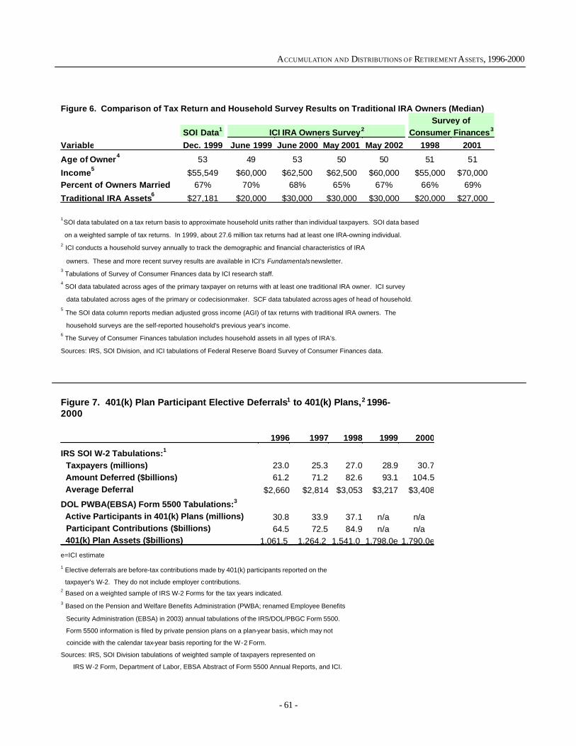
- 61 -
ACCUMULATION AND DISTRIBUTIONS OF RETIREMENT ASSETS, 1996-2000
Figure 6. Comparison of Tax Return and Household Survey Results on Traditional IRA Owners (Median) Survey of SOI Data1 ICI IRA Owners Survey2 Consumer Finances3 Variable Dec. 1999 June 1999 June 2000 May 2001 May 2002 1998 2001
Age of Owner4 53 49 53 50 50 51 51
Income5 $55,549 $60,000 $62,500 $62,500 $60,000 $55,000 $70,000 Percent of Owners Married 67% 70% 68% 65% 67% 66% 69%
Traditional IRA Assets6 $27,181 $20,000 $30,000 $30,000 $30,000 $20,000 $27,000 1SOI data tabulated on a tax return basis to approximate household units rather than individual taxpayers. SOI data based
on a weighted sample of tax returns. In 1999, about 27.6 million tax returns had at least one IRA-owning individual. 2 ICI conducts a household survey annually to track the demographic and financial characteristics of IRA
owners. These and more recent survey results are available in ICI's Fundamentals newsletter. 3
Tabulations of Survey of Consumer Finances data by ICI research staff. 4
SOI data tabulated across ages of the primary taxpayer on returns with at least one traditional IRA owner. ICI survey
data tabulated across ages of the primary or codecisionmaker. SCF data tabulated across ages of head of household. 5 The SOI data column reports median adjusted gross income (AGI) of tax returns with traditional IRA owners. The
household surveys are the self-reported household's previous year's income. 6
The Survey of Consumer Finances tabulation includes household assets in all types of IRA’s.
Sources: IRS, SOI Division, and ICI tabulations of Federal Reserve Board Survey of Consumer Finances data.
Figure 7. 401(k) Plan Participant Elective Deferrals1 to 401(k) Plans,2 1996-2000 1996 1997 1998 1999 2000
IRS SOI W-2 Tabulations:1 Taxpayers (millions) 23.0 25.3 27.0 28.9 30.7 Amount Deferred ($billions) 61.2 71.2 82.6 93.1 104.5 Average Deferral $2,660 $2,814 $3,053 $3,217 $3,408
DOL PWBA(EBSA) Form 5500 Tabulations:3 Active Participants in 401(k) Plans (millions) 30.8 33.9 37.1 n/a n/a Participant Contributions ($billions) 64.5 72.5 84.9 n/a n/a 401(k) Plan Assets ($billions) 1,061.5 1,264.2 1,541.0 1,798.0e 1,790.0e
e=ICI estimate 1 Elective deferrals are before-tax contributions made by 401(k) participants reported on the
taxpayer's W-2. They do not include employer contributions. 2 Based on a weighted sample of IRS W-2 Forms for the tax years indicated. 3 Based on the Pension and Welfare Benefits Administration (PWBA; renamed Employee Benefits
Security Administration (EBSA) in 2003) annual tabulations of the IRS/DOL/PBGC Form 5500.
Form 5500 information is filed by private pension plans on a plan-year basis, which may not
coincide with the calendar tax-year basis reporting for the W-2 Form.
Sources: IRS, SOI Division tabulations of weighted sample of taxpayers represented on
IRS W-2 Form, Department of Labor, EBSA Abstract of Form 5500 Annual Reports, and ICI.
- 63 -
The Effects of Tax Reform on the Structureof U.S. Business
Ellen Legel, Kelly Bennett, and Michael Parisi, Internal Revenue Service
T he 1990’s have been described as a period ofimmense and protracted profit-taking in the stockmarket. Mergers and acquisitions have impacted
business demographics. Tax law changes have also hada marked effect by continually providing incentives anddisincentives for certain business legal forms of owner-ship, such as those affecting the growth rates of compa-nies moving from corporate to noncorporate status. Lawchanges, such as the landmark 1986 Tax Reform Act,the Small Business Job Protection Act of 1996, and theOmnibus Reconciliation Act of 1997, have had signifi-cant impacts on Subchapter C corporations, includingsmall business (or Subchapter S) corporations; partner-ships (general, limited, and limited liability companiesLLC’s); and sole proprietorships.
This paper is an examination of the changes in busi-ness demographics or “business organizational choice”of the various types of business during the 1990’s andthe changes in the historical trend from the 1980 period.Tax data will be used to focus on changes in the variousbusiness types, receipts, profitability, and tax rates overtwo recessions due to modifications in the tax code onadministrative records sampled at Statistics of Income(SOI) Division of IRS.
The paper is divided into three sections. The firstdefines the various types of businesses. The secondexplains tax law changes during the 1990’s. The thirdanalyzes a time series dataset for the three distinct busi-ness types (and their subsets) based on tax filings withthe IRS.
� Organizational Type
For this paper, corporations are divided into C cor-porations, those taxed at corporate rates, and S corpora-tions, those taxed at individual income tax rates. Part-nerships are divided into general partnerships, limitedpartnerships, and limited liability companies (LLC’s).Since the tax treatment of the business organizationalforms varies significantly, a brief synopsis follows.
Corporations. Corporation (or Subchapter C) in-come is generally taxed directly at the business level,and again at the shareholder level for receipt of dividendincome. Income distributed to shareholders is only tax-able on the after-tax profits earned by the corporation.However, after-tax corporate income is taxable at theshareholder level once it is distributed as dividends orthe shareholder realizes capital gain.
Subchapter S. S corporations are incorporated en-tities that have many of the same attributes as the tradi-tional C corporation, including limited liability, freely trans-ferable ownership, and unlimited life span. Unlike the Ccorporations, income and losses are passed through tothe shareholder and are subject to tax only at the ownerlevel. S corporation shareholders report their shares ofincome or loss on their own tax returns. Therefore, anyresulting tax liability is the responsibility of the share-holders. S corporations offer the benefits of partnershiptaxation without the liability. Subchapter S corporationsmust be compared with the limited liability company(LLC), which they resemble in operation and concept.Despite having several appealing characteristics, S cor-porations do face inherent limitations, including the num-ber and type of shareholders, permitting only one classof stock, and exclusion of foreign, corporate, partner-ship, or LLC ownership.
Partnerships. Similar to the S corporation, a part-nership does not pay tax on its income but passes throughany income or losses to its partners. Partners includethis passthrough income on their tax returns.
Partnerships may be general partnerships, limitedpartnerships, limited liability partnerships, and limited li-ability companies. Creditors of general partnerships,composed solely of general partners, may collect amountsowed to them from both the general partnership assetsand the assets of the general partners. General partnersare personally liable, limited to their personal resources,and actively participate in management of the business.Limited partnerships (LP’s) have at least one general
- 64 -
LEGEL, BENNETT, AND PARISI
partner. A limited partner is similar to a corporate share-holder, whose liability to third-party creditors is limited tothe amount invested in the partnership. Limited liabilitypartnerships (LLP’s) are formed under State-limited li-ability partnership law. Limited liability partners, whoseowners are general partners, are not personally liablefor the debts of the LLP or any other partner, nor is thepartner liable for the malpractice committed by otherpartners.
Limited liability companies (LLC’s). The LLCis a State-formed entity with the limited liability of a cor-poration and the tax liability of a partnership. This hy-brid entity has quickly become an alternative to the tra-ditional partnership and corporate business structures.The members of the LLC are treated similarly to limitedpartners, in that income passes through an LLC to themembers. The members include this passthrough in-come on their tax returns. Unlike general partners, themembers of the LLC are not personally liable for theLLC’s debts.
Data from LLC’s have been collected since theirfirst appearance on the partnership annual informationreturn in 1993. LLC’s are required to file on the part-nership annual information return (Form 1065), althoughsome file on the S corporation return. The LLC datadisplayed in this article are representative of the datagathered from the partnership annual information returnonly.
Sole Proprietorships. An owner of a non-farmsole-proprietorship summarizes the income and expensesof the business on Schedule C (or C-EZ) of the owner’sindividual income (Form 1040) tax return. The net in-come or loss from the business is added to the owner’spersonal income from all other sources and taxed at theapplicable individual income tax rates.
� Tax Law Changes
The Tax Reform Act of 1986 (TRA86), the mostcomprehensive revision of the Internal Revenue Codesince 1954, had a major impact on business decisions inthe period after 1986 by broadening the tax base of bothindividuals and corporations by tightening the corpora-tion “alternative minimum tax,” limiting losses from pas-
sive activities, and repealing the long-term capital gainexclusion. The most marked effect has been on thechanges in the individual and corporate marginal tax rates.In pre-TRA86, the highest individual rate (50 percent)exceeded the highest corporation rate (46 percent) by 4percentage points.
TRA86 reversed this trend, starting in 1987 and con-tinuing with the final lowered rates of 1988-1990 of 34percent for corporations and 28 percent for individuals,a 6-percentage point reversal. For 1991 and 1992, thisdifference was cut in half when the individual rate wasincreased to 31 percent (Figure A).
In 1993 to the present, the top individual rate in-creased to 39.6 percent surpassing the highest corpora-tion rate of 35 percent. Although both rates are lowerthan pre-TRA86, the difference of 4.6 percentage pointsbetween the individual rate and the corporation rate looksalmost identical to the pre-TRA86 difference of 4 per-centage points. The incentive to switch business typesdeclined and reversed. With the reversal in incentives,was there renewed interest in the corporation type ofbusiness? We will investigate, using the SOI data for1990-2000 for all three types of business entities.
Figure A. Top Marginal Tax Rates (Percentages) Corporations and Individuals, 1990-2000
Item 1990 1991-1992 1993-2000 Corporations 34.0 34.0 35.0 Individuals 28.0 31.0 39.6 Difference 6.0 3.0 -4.6 Note: These rates are for the highest levels of taxable income and do not reflect alternative minimum tax.
The Small Business Job Protection Act of 1996(SBJPA) made several noteworthy changes that havesignificantly affected S corporation filings. First, theSBJPA increased the maximum number of shareholdersfrom 35 to 75. Second, it enabled financial institutions,which did not use the reserve method of accounting forbad debts, to make an S election. Third, small business
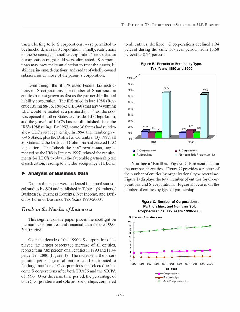
- 65 -
THE EFFECTS OF TAX REFORM ON THE STRUCTURE OF U.S. BUSINESS
trusts electing to be S corporations, were permitted tobe shareholders in an S corporation. Finally, restrictionson the percentage of another corporation’s stock that anS corporation might hold were eliminated. S corpora-tions may now make an election to treat the assets, li-abilities, income, deductions, and credits of wholly-ownedsubsidiaries as those of the parent S corporation.
Even though the SBJPA eased Federal tax restric-tions on S corporations, the number of S corporationentities has not grown as fast as the partnership limitedliability corporation. The IRS ruled in late 1988 (Rev-enue Ruling 88-76, 1988-2 C.B.360) that any WyomingLLC would be treated as a partnership. Thus, the doorwas opened for other States to consider LLC legislation,and the growth of LLC’s has not diminished since theIRS’s 1988 ruling. By 1993, some 36 States had ruled toallow LLC’s as a legal entity. In 1994, that number grewto 46 States, plus the District of Columbia. By 1997, all50 States and the District of Columbia had enacted LLClegislation. The “check-the-box” regulations, imple-mented by the IRS in January 1997, relaxed the require-ments for LLC’s to obtain the favorable partnership taxclassification, leading to a wider acceptance of LLC’s.
� Analysis of Business Data
Data in this paper were collected in annual statisti-cal studies by SOI and published in Table 1 (Number ofBusinesses, Business Receipts, Net Income, and Defi-cit by Form of Business, Tax Years 1990-2000).
Trends in the Number of Businesses
This segment of the paper places the spotlight onthe number of entities and financial data for the 1990-2000 period.
Over the decade of the 1990’s S corporations dis-played the largest percentage increase of all entities,representing 7.85 percent of all entities in 1990 and 11.44percent in 2000 (Figure B). The increase in the S cor-poration percentage of all entities can be attributed tothe large number of C corporations that elected to be-come S corporations after both TRA86 and the SBJPAof 1996. Over the same time period, the percentage ofboth C corporations and sole proprietorships, compared
to all entities, declined. C corporations declined 1.94percent during the same 10- year period, from 10.68percent to 8.74 percent.
10.687.85
7.75
73.72
8.7411.44
8.23
71.60
0%
10%
20%
30%
40%
50%
60%
70%
80%
90%
100%
1990 2000
Figure B. Percent of Entities by Type,Tax Years 1990 and 2000
C Corporations S Corporations Partnerships Nonfarm Sole Proprietorships
Number of Entities. Figures C-E present data onthe number of entities. Figure C provides a picture ofthe number of entities by organizational type over time.Figure D displays the total number of entities for C cor-porations and S corporations. Figure E focuses on thenumber of entities by type of partnership.
Figure C. Number of Corporations, Partnerships, and Nonfarm Sole
Proprietorships, Tax Years 1990-2000
02468
101214161820
1990 1991 1992 1993 1994 1995 1996 1997 1998 1999 2000
T ax YearCorporationsPartnershipsSo le Proprietorships
M illio ns o f businesses
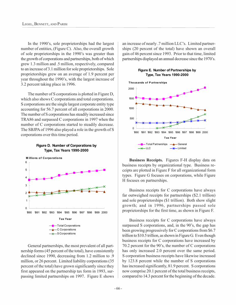
- 66 -
LEGEL, BENNETT, AND PARISI
In the 1990’s, sole proprietorships had the largestnumber of entities, (Figure C). Also, the overall growthof sole proprietorships in the 1990’s was greater thanthe growth of corporations and partnerships, both of whichgrew 1.3 million and .5 million, respectively, comparedto an increase of 3.1 million for sole proprietorships. Soleproprietorships grew on an average of 1.9 percent peryear throughout the 1990’s, with the largest increase of3.2 percent taking place in 1996.
The number of S corporations is plotted in Figure D,which also shows C corporations and total corporations.S corporations are the single largest corporate entity typeaccounting for 56.7 percent of all corporations in 2000.The number of S corporations has steadily increased sinceTRA86 and surpassed C corporations in 1997 when thenumber of C corporations started to steadily decrease.The SBJPA of 1996 also played a role in the growth of Scorporations over this time period.
an increase of nearly .7 million LLC’s. Limited partner-ships (20 percent of the total) have shown an overallgain of 46 percent since 1993. Prior to that time, limitedpartnerships displayed an annual decrease since the 1970’s.
Figure D. Number of Corporations by Type, Tax Years 1990-2000
0
1
2
3
4
5
6
1990 1991 1992 1993 1994 1995 1996 1997 1998 1999 2000
Tax Year
Total CorporationsC CorporationsS Corporations
M illions o f Corporations
General partnerships, the most prevalent of all part-nership forms (45 percent of the total), have consistentlydeclined since 1990, decreasing from 1.2 million to .9million, or 26 percent. Limited liability corporations (35percent of the total) have grown significantly since theyfirst appeared on the partnership tax form in 1993, sur-passing limited partnerships on 1997. Figure E shows
Figure E. Number of Partnerships by Type, Tax Years 1990-2000
0
500
1000
1500
2000
1990 1991 1992 1993 1994 1995 1996 1997 1998 1999 2000
T ax Year
Total Partnerships GeneralLLC Limited
T housands o f P artnerships
Business Receipts. Figures F-H display data onbusiness receipts by organizational type. Business re-ceipts are plotted in Figure F for all organizational formtypes. Figure G focuses on corporations, while FigureH focuses on partnerships.
Business receipts for C corporations have alwaysfar outweighed receipts for partnerships ($2.1 trillion)and sole proprietorships ($1 trillion). Both show slightgrowth; and in 1996, partnerships passed soleproprietorships for the first time, as shown in Figure F.
Business receipts for C corporations have alwayssurpassed S corporations, and, in the 90’s, the gap hasbeen growing progressively for C corporations from $6.7trillion to $10.5 trillion, as shown in Figure G. Even thoughbusiness receipts for C corporations have increased by70.2 percent for the 90’s, the number of C corporationshas only increased 2.0 percent over the same period.S corporation business receipts have likewise increasedby 123.8 percent while the number of S corporationshas increased significantly, 81.9 percent. S corporationsnow comprise 20.1 percent of the total business receipts,compared to 14.3 percent for the beginning of the decade.
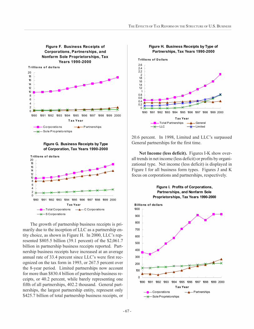
- 67 -
THE EFFECTS OF TAX REFORM ON THE STRUCTURE OF U.S. BUSINESS
The growth of partnership business receipts is pri-marily due to the inception of LLC as a partnership en-tity choice, as shown in Figure H. In 2000, LLC’s rep-resented $805.5 billion (39.1 percent) of the $2,061.7billion in partnership business receipts reported. Part-nership business receipts have increased at an averageannual rate of 33.4 percent since LLC’s were first rec-ognized on the tax form in 1993, or 267.5 percent overthe 8-year period. Limited partnerships now accountfor more than $830.4 billion of partnership business re-ceipts, or 40.2 percent, while barely representing onefifth of all partnerships, 402.2 thousand. General part-nerships, the largest partnership entity, represent only$425.7 billion of total partnership business receipts, or
20.6 percent. In 1998, Limited and LLC’s surpassedGeneral partnerships for the first time.
Net Income (less deficit). Figures I-K show over-all trends in net income (less deficit) or profits by organi-zational type. Net income (less deficit) is displayed inFigure I for all business form types. Figures J and Kfocus on corporations and partnerships, respectively.
Figure F. Business Receipts of Corporations, Partnerships, and
Nonfarm Sole Proprietorships, Tax Years 1990-2000
02468
101214161820
1990 1991 1992 1993 1994 1995 1996 1997 1998 1999 2000
T a x Y e a r
Co rpo ratio ns P artnershipsSo le P ro prieto rships
T rillio ns o f do lla rs
Figure G. Business Receipts by Type of Corporation, Tax Years 1990-2000
02468
101214161820
1990 1991 1992 1993 1994 1995 1996 1997 1998 1999 2000
T ax YearTotal Corporations C CorporationsS Corporations
T rillio ns o f do llars
Figure H. Business Receipts by Type of Partnerships, Tax Years 1990-2000
00.20.40.60.8
11.21.41.61.82
2.22.42.6
1990 1991 1992 1993 1994 1995 1996 1997 1998 1999 2000
T ax YearTotal Partnerships GeneralLLC Limited
T rillio ns o f D o llars
Figure I. Profits of Corporations, Partnerships, and Nonfarm Sole
Proprietorships, Tax Years 1990-2000
0
100
200
300
400
500
600
700
800
900
1000
1990 1991 1992 1993 1994 1995 1996 1997 1998 1999 2000Tax Year
Corporations PartnershipsSole Proprietorships
Billions o f do llars
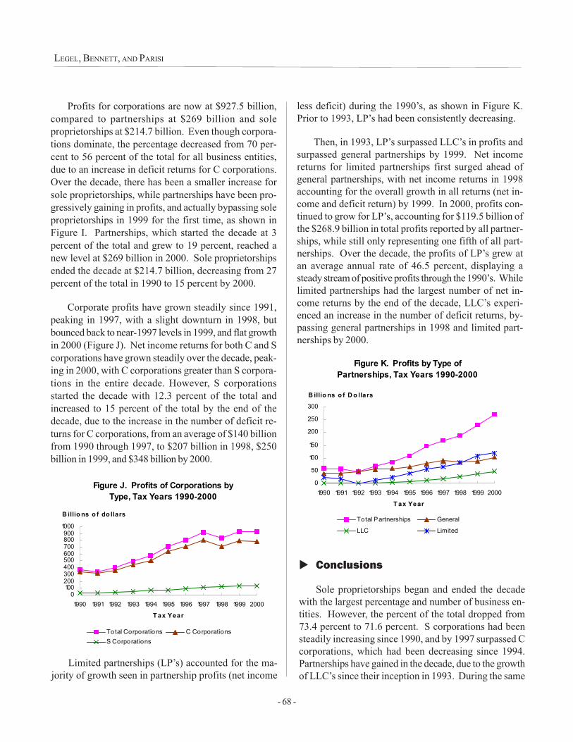
- 68 -
LEGEL, BENNETT, AND PARISI
Profits for corporations are now at $927.5 billion,compared to partnerships at $269 billion and soleproprietorships at $214.7 billion. Even though corpora-tions dominate, the percentage decreased from 70 per-cent to 56 percent of the total for all business entities,due to an increase in deficit returns for C corporations.Over the decade, there has been a smaller increase forsole proprietorships, while partnerships have been pro-gressively gaining in profits, and actually bypassing soleproprietorships in 1999 for the first time, as shown inFigure I. Partnerships, which started the decade at 3percent of the total and grew to 19 percent, reached anew level at $269 billion in 2000. Sole proprietorshipsended the decade at $214.7 billion, decreasing from 27percent of the total in 1990 to 15 percent by 2000.
Corporate profits have grown steadily since 1991,peaking in 1997, with a slight downturn in 1998, butbounced back to near-1997 levels in 1999, and flat growthin 2000 (Figure J). Net income returns for both C and Scorporations have grown steadily over the decade, peak-ing in 2000, with C corporations greater than S corpora-tions in the entire decade. However, S corporationsstarted the decade with 12.3 percent of the total andincreased to 15 percent of the total by the end of thedecade, due to the increase in the number of deficit re-turns for C corporations, from an average of $140 billionfrom 1990 through 1997, to $207 billion in 1998, $250billion in 1999, and $348 billion by 2000.
less deficit) during the 1990’s, as shown in Figure K.Prior to 1993, LP’s had been consistently decreasing.
Then, in 1993, LP’s surpassed LLC’s in profits andsurpassed general partnerships by 1999. Net incomereturns for limited partnerships first surged ahead ofgeneral partnerships, with net income returns in 1998accounting for the overall growth in all returns (net in-come and deficit return) by 1999. In 2000, profits con-tinued to grow for LP’s, accounting for $119.5 billion ofthe $268.9 billion in total profits reported by all partner-ships, while still only representing one fifth of all part-nerships. Over the decade, the profits of LP’s grew atan average annual rate of 46.5 percent, displaying asteady stream of positive profits through the 1990’s. Whilelimited partnerships had the largest number of net in-come returns by the end of the decade, LLC’s experi-enced an increase in the number of deficit returns, by-passing general partnerships in 1998 and limited part-nerships by 2000.
Figure J. Profits of Corporations by Type, Tax Years 1990-2000
0100200300400500600700800900
1000
1990 1991 1992 1993 1994 1995 1996 1997 1998 1999 2000
T ax Year
Total Corporations C CorporationsS Corporations
B illio ns o f do llars
Figure K. Profits by Type of Partnerships, Tax Years 1990-2000
0
50
100
150
200
250
300
1990 1991 1992 1993 1994 1995 1996 1997 1998 1999 2000
T ax Year
Total Partnerships General
LLC Limited
B illio ns o f D o llars
� Conclusions
Sole proprietorships began and ended the decadewith the largest percentage and number of business en-tities. However, the percent of the total dropped from73.4 percent to 71.6 percent. S corporations had beensteadily increasing since 1990, and by 1997 surpassed Ccorporations, which had been decreasing since 1994.Partnerships have gained in the decade, due to the growthof LLC’s since their inception in 1993. During the same
Limited partnerships (LP’s) accounted for the ma-jority of growth seen in partnership profits (net income
- 69 -
THE EFFECTS OF TAX REFORM ON THE STRUCTURE OF U.S. BUSINESS
time, general partnerships have been on a gradual down-ward turn.
The most obvious reason for the increase in LLC’sis their advantages over other business entity types. Allmembers of LLC’s have the same limited liability pro-tection; by comparison, a partnership must have at leastone general partner that does not have limited liability.LLC’s offer flexible management and flexible owner-ship, allowing members to participate in the LLC’s man-agement without exposing themselves to possible per-sonal liability. LLC’s offer several advantages over Scorporations since there is no limitation on the numberof owners, type of owners, or on the allowable types ofinterest. S corporations are limited to seventy-five share-holders, none of which can be nonresident aliens, andmay only have one class of stock. The flexibility that anLLC offers helps attract a broader range of businessinvestors than is possible with an S corporation.
The business receipts of corporations outdistancedpartnerships and sole proprietorships due to the domi-nance of C corporations. However, C corporations havedropped from 86 percent of the total receipts of all corpo-rations to 83 percent by the end of the decade. Generalpartnerships have been decreasing since 1997, and by1998 were surpassed by LLC’s and limited partnerships.
For net income (less deficit) returns, C corporationsare the largest of all entities, but dropped from 64 per-cent to 56 percent by 2000. Net income rose for allcorporations due to C corporations, with the gap in thegrowth rate widening over S corporations. Partnershipincome also rose due to the steady increase in incomefor limited partnerships that surpassed general partner-ships by 1999.
For C corporations, there has been a 68-percent in-crease in deficit returns since 1998. Likewise, for part-nerships, losses have been increasing since 1994. Gen-eral partnerships were surpassed by LLC’s in 1998, andby limited partnerships by 2000.
Two factors accounted for the growth in S corpora-tions and LLC’s. In 1994, the number of States, 36, thatpermitted the formation of LLC’s commenced a 7-yearrise in the number of partnerships. The passage of the
Small Business Job Protection Act (SBJPA96) increasedthe number of allowable shareholders from 35 to 75, andcontributed to the growth of S corporations over C cor-porations, especially in the smaller asset categories. Bothof these factors allowed income to be passed on to theindividual and taxed at the lower individual rate ratherthan at the corporate rate.
� References
Bennett, Kelly, “S Corporation Returns, 2000,” Statis-tics of Income Bulletin, Spring 2003, Volume 22,Number 4 (as well as Bulletin articles on theseorganizations for other years).
Gill, Amy and Wittman, Susan, “S Corporation Elec-tions After the Tax Reform Act of 1986,” Statis-tics of Income Bulletin, Spring 1998, Volume 17,Number 4.
Manolakas, Thomas G. (2000), Partnerships andLLC’s Tax Practice and Analysis, CCH Incorpo-rated, Chicago.
Petska, Tom, “Taxes and Business OrganizationalChoice: Déjà Vu All Over Again?”
Petska, Tom, “Taxes and Organizational Choice: AnAnalysis of Trends, 1985-1992,” Statistics of In-come Bulletin, Spring 1996, Volume 15, Number 4.
Pratt, William, “Partnership Returns, 2000,” Statisticsof Income Bulletin, Fall, 2002, Volume 22, Num-ber 2 (as well as Bulletin articles on these organi-zations for other years).
Schlesinger, Michael (2000), S Corporations Tax Prac-tice and Analysis, CCH Incorporated, Chicago.
Acknowledgment
The authors would like to extend special thanks to:Patrice Treubert, for developing the SAS data set; Bill Prattand Tim Wheeler, for producing the partnership data. Thisarticle was a continuation of The Effects of Tax Re-form on the Structure of U.S. Business, written by TomPetska. Any errors are the responsibility of the authors.
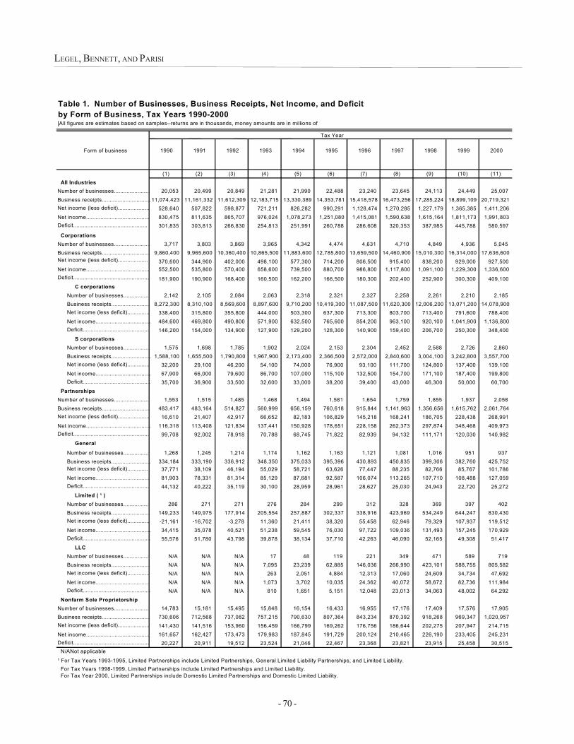
- 70 -
LEGEL, BENNETT, AND PARISI
Table 1. Number of Businesses, Business Receipts, Net Income, and Deficit by Form of Business, Tax Years 1990-2000 [All figures are estimates based on samples--returns are in thousands, money amounts are in millions of
Tax Year
Form of business 1990 1991 1992 1993 1994 1995 1996 1997 1998 1999 2000
(1) (2) (3) (4) (5) (6) (7) (8) (9) (10) (11) All Industries Number of businesses....................... 20,053 20,499 20,849 21,281 21,990 22,488 23,240 23,645 24,113 24,449 25,007 Business receipts............................... 11,074,423 11,161,332 11,612,309 12,183,715 13,330,389 14,353,781 15,418,578 16,473,256 17,285,224 18,899,109 20,719,321 Net income (less deficit).................... 528,640 507,822 598,877 721,211 826,282 990,291 1,128,474 1,270,285 1,227,179 1,365,385 1,411,206 Net income........................................ 830,475 811,635 865,707 976,024 1,078,273 1,251,080 1,415,081 1,590,638 1,615,164 1,811,173 1,991,803 Deficit............................................... 301,835 303,813 266,830 254,813 251,991 260,788 286,608 320,353 387,985 445,788 580,597
Corporations Number of businesses...................… 3,717 3,803 3,869 3,965 4,342 4,474 4,631 4,710 4,849 4,936 5,045 Business receipts.............................. 9,860,400 9,965,600 10,360,400 10,865,500 11,883,600 12,785,800 13,659,500 14,460,900 15,010,300 16,314,000 17,636,600 Net income (less deficit)................... 370,600 344,900 402,000 498,100 577,300 714,200 806,500 915,400 838,200 929,000 927,500 Net income........................................ 552,500 535,800 570,400 658,600 739,500 880,700 986,800 1,117,800 1,091,100 1,229,300 1,336,600 Deficit................................................ 181,900 190,900 168,400 160,500 162,200 166,500 180,300 202,400 252,900 300,300 409,100 C corporations Number of businesses................ 2,142 2,105 2,084 2,063 2,318 2,321 2,327 2,258 2,261 2,210 2,185 Business receipts........................ 8,272,300 8,310,100 8,569,600 8,897,600 9,710,200 10,419,300 11,087,500 11,620,300 12,006,200 13,071,200 14,078,900 Net income (less deficit).............. 338,400 315,800 355,800 444,000 503,300 637,300 713,300 803,700 713,400 791,600 788,400 Net income................................... 484,600 469,800 490,800 571,900 632,500 765,600 854,200 963,100 920,100 1,041,900 1,136,800 Deficit.......................................... 146,200 154,000 134,900 127,900 129,200 128,300 140,900 159,400 206,700 250,300 348,400 S corporations Number of businesses................. 1,575 1,698 1,785 1,902 2,024 2,153 2,304 2,452 2,588 2,726 2,860 Business receipts......................... 1,588,100 1,655,500 1,790,800 1,967,900 2,173,400 2,366,500 2,572,000 2,840,600 3,004,100 3,242,800 3,557,700 Net income (less deficit).............. 32,200 29,100 46,200 54,100 74,000 76,900 93,100 111,700 124,800 137,400 139,100 Net income................................... 67,900 66,000 79,600 86,700 107,000 115,100 132,500 154,700 171,100 187,400 199,800 Deficit........................................... 35,700 36,900 33,500 32,600 33,000 38,200 39,400 43,000 46,300 50,000 60,700 Partnerships Number of businesses...................... 1,553 1,515 1,485 1,468 1,494 1,581 1,654 1,759 1,855 1,937 2,058 Business receipts.............................. 483,417 483,164 514,827 560,999 656,159 760,618 915,844 1,141,963 1,356,656 1,615,762 2,061,764 Net income (less deficit).................... 16,610 21,407 42,917 66,652 82,183 106,829 145,218 168,241 186,705 228,438 268,991 Net income......................................... 116,318 113,408 121,834 137,441 150,928 178,651 228,158 262,373 297,874 348,468 409,973 Deficit................................................ 99,708 92,002 78,918 70,788 68,745 71,822 82,939 94,132 111,171 120,030 140,982 General Number of businesses................ 1,268 1,245 1,214 1,174 1,162 1,163 1,121 1,081 1,016 951 937 Business receipts......................... 334,184 333,190 336,912 348,350 375,033 395,396 430,893 450,835 399,306 382,760 425,752 Net income (less deficit)............. 37,771 38,109 46,194 55,029 58,721 63,626 77,447 88,235 82,766 85,767 101,786 Net income.................................. 81,903 78,331 81,314 85,129 87,681 92,587 106,074 113,265 107,710 108,488 127,059 Deficit.......................................... 44,132 40,222 35,119 30,100 28,959 28,961 28,627 25,030 24,943 22,720 25,272 Limited ( ¹ ) Number of businesses................ 286 271 271 276 284 299 312 328 369 397 402 Business receipts........................ 149,233 149,975 177,914 205,554 257,887 302,337 338,916 423,969 534,249 644,247 830,430 Net income (less deficit).............. -21,161 -16,702 -3,278 11,360 21,411 38,320 55,458 62,946 79,329 107,937 119,512 Net income................................... 34,415 35,078 40,521 51,238 59,545 76,030 97,722 109,036 131,493 157,245 170,929 Deficit........................................... 55,576 51,780 43,798 39,878 38,134 37,710 42,263 46,090 52,165 49,308 51,417 LLC Number of businesses................ N/A N/A N/A 17 48 119 221 349 471 589 719 Business receipts........................ N/A N/A N/A 7,095 23,239 62,885 146,036 266,990 423,101 588,755 805,582 Net income (less deficit).............. N/A N/A N/A 263 2,051 4,884 12,313 17,060 24,609 34,734 47,692 Net income.................................. N/A N/A N/A 1,073 3,702 10,035 24,362 40,072 58,672 82,736 111,984 Deficit........................................... N/A N/A N/A 810 1,651 5,151 12,048 23,013 34,063 48,002 64,292 Nonfarm Sole Proprietorship Number of businesses...................... 14,783 15,181 15,495 15,848 16,154 16,433 16,955 17,176 17,409 17,576 17,905 Business receipts.............................. 730,606 712,568 737,082 757,215 790,630 807,364 843,234 870,392 918,268 969,347 1,020,957 Net income (less deficit).................... 141,430 141,516 153,960 156,459 166,799 169,262 176,756 186,644 202,275 207,947 214,715 Net income........................................ 161,657 162,427 173,473 179,983 187,845 191,729 200,124 210,465 226,190 233,405 245,231 Deficit................................................ 20,227 20,911 19,512 23,524 21,046 22,467 23,368 23,821 23,915 25,458 30,515 N/ANot applicable ¹ For Tax Years 1993-1995, Limited Partnerships include Limited Partnerships, General Limited Liability Partnerships, and Limited Liability. For Tax Years 1998-1999, Limited Partnerships include Limited Partnerships and Limited Liability. For Tax Year 2000, Limited Partnerships include Domestic Limited Partnerships and Domestic Limited Liability.
- 71 -
Statistical Information Services at IRS: ImprovingDissemination of Data and Satisfying the Customer
Beth Kilss and David Jordan, Internal Revenue Service
IRS�s Statistics of Income (SOI) Division conductsstatistical studies on the operations of the tax laws andpublishes annual reports on corporations and individuals,the quarterly SOI Bulletin, an annual research report,special periodic reports and compendiums, and the an-nual IRS Data Book. The IRS World Wide Web siteprovides users an easy option for accessing these re-ports and other SOI data and also serves as a conduitfor releasing other IRS information. Periodic news re-leases to the mainstream media announcing key prod-ucts raise awareness of the data SOI makes available tothe public. SOI�s Statistical Information Services (SIS)office, comprised of statisticians and economists, has em-phasized top-quality, customer-focused service through-out its 14-year history and strives to provide timely, ac-curate, and well-documented guidance on the availabil-ity of SOI data and other statistical services.
This paper will provide an overview of SOI effortsto improve and expand data dissemination. In the firstsection of the paper, some background information aboutthe SOI Division and its Statistical Information Servicesoffice is highlighted and outlined. The second sectiondiscusses recent improvements to SOI�s web site. Thethird section looks at innovations in data disseminationthrough the web site, the SIS office, and news releases.In the last section, some results from a recent survey ofSIS customers are presented, along with how SOI isusing these results to identify problem areas and improvecustomer service.
� Background Information
Congress created the Statistics of Income Divisionnearly 90 years ago in the Revenue Act of 1916, some 3years after the enactment of the modern income tax in1913. Since that time, the Internal Revenue Code hasincluded virtually the same language mandating the prepa-ration of statistics. Section 6108 of the Code currentlystates that ��the Secretary (of the Treasury) shall pre-pare and publish not less than annually statistics reason-ably available with respect to the operations of the inter-
nal revenue laws, including classifications of taxpayersand of income, the amounts claimed or allowed as de-ductions, exemptions, and credits.�
SOI�s mission is to collect, analyze, and disseminateinformation on Federal taxation for the Office of TaxAnalysis, Congressional Committees, the Internal Rev-enue Service in its administration of the tax laws, otherorganizations engaged in economic and financial analy-sis, and the general public. Its mission is similar to thatof other Federal statistical agencies�that is, to collectand process data so that they become useful and mean-ingful information. However, SOI collects data fromtax returns rather than through surveys, as do most otherstatistical agencies. These data are processed and pro-vided to customers, in the form of tabulations or microdatafiles. Although the IRS uses SOI data, the primary usesfor SOI data are outside of IRS, in policy analyses de-signed to study the effects of new or proposed tax lawsand in evaluating the functioning of the U.S. economy.
Throughout its long history, SOI�s main emphasis hasbeen individual and corporation income tax information.However, growth has occurred over the years in thenature and number of studies undertaken. In addition toindividuals and corporations, SOI Division also conductsstatistical studies on partnerships, sole proprietorships,estates, nonprofit organizations, and trusts, as well asspecial projects or studies of international activities. In1980, the SOI program consisted of 26 projects; now, in2003, the SOI program consists of over 60 projects. Whilethe number of projects has more than doubled over thepast 20 years, this growth has been accompanied by evenlarger increases in the amount of data extracted fromthe various tax and information returns during that sametimeframe.
SOI Products and Services. Statistics of Incomeinformation reaches thousands of outside tax practitio-ners and researchers, State and local governments, themedia, the public at large, and staff within the IRS itselfthrough SOI�s published products and electronic media.
- 72 -
KILSS AND JORDAN
SOI user inquiries come from a wide array of interests.The detailed income and expenditure data provided ontax and information returns are highly regarded and morereliable than similar survey data because there are pen-alties for misreporting. SOI information is published inthe quarterly Statistics of Income Bulletin, which con-tains four to eight articles and data releases of recentlycompleted studies, as well as historical tables covering avariety of subject matter; separate annual �completereports� on individual and corporation income tax re-turns, which contain more comprehensive data than thosepublished in the Bulletin; and the annual CorporationSource Book, which presents detailed income statement,balance sheet, and tax data by industry and asset size.
Other SOI publications include special compendi-ums of research, which are published periodically on suchtopics as nonprofit organizations and estate taxation andpersonal wealth, and research articles published in a se-ries of reports, usually annually, which document tech-nological and methodological changes in SOI programsand other related statistical uses of administrativerecords. More recently, SOI Division has become thepublisher of the Internal Revenue Service Data Bookand the IRS Office of Research�s annual research con-ference proceedings.
The IRS World Wide Web site offers easy accessto these products and other services free of charge atwww.irs.gov/taxstats. More specifically, at this site,users will find a combination of files presenting tax-re-lated data on individuals, corporations, and other enti-ties; articles about SOI data; information about SOI prod-ucts and services; and non-SOI products, including theData Book, Compliance Research projections, and non-profit Master File microdata records. At present, over1,734 files reside there.
Statistical Information Services Office. Over 14years ago, SOI created its Statistical Information Ser-vices (SIS) Office to facilitate the dissemination of SOIdata and reports and respond to all data and informationrequests. This office was established as a direct resultof the management study mandated by the Office ofManagement and Budget Circular A-76 process in thelate 1980�s, which required SOI Division to determineits �most efficient organization.� The establishment of
the SIS office was one of a number of recommenda-tions coming out of the A-76 process. Within 2 years ofthe decision to centralize responses to all data and infor-mation requests received in SOI, the SIS office openedfor business in early 1989.
During the first 5 years, there was a steady increaseeach year in the number of telephone and written re-quests for SOI data and publications. Little by little, theSIS office began to establish a reputation for alwaysproviding an answer or at least a referral to someonewho could provide an answer. In the midst of buildingup reference materials, setting up a library, and trainingnew staff to help handle the growing workload, the tech-nologies available were also changing. Word proces-sors, typewriters, photocopy machines, and telephonewere the main tools used to support this work at thebeginning. Fortunately, within a few years, a computer-ized system for tracking and recording all customer re-quests was designed and implemented. The system isperiodically updated and refined to keep pace with thechanging functionalities of the SIS office, and it is usedto permanently record all requests received, invoice cus-tomers for reimbursable products, and generate variousreports about customers and their requests.
In more recent years, SOI has expanded the SISfunction to better serve the public, first, by means of anelectronic bulletin board (in 1992), and, more recently,by participating with the rest of IRS on the World WideWeb (in 1996). As electronic dissemination has growndramatically, the number of written and telephone re-quests has declined, but questions that do not lend them-selves to answers over the Internet have grown morecomplicated.
The current SIS staff handled nearly 2,800 informa-tion requests in Calendar Year 2002, and an equal num-ber in Fiscal Year 2003. During FY 2003, about half ofthe requests were received from e-mails and faxes, whileabout 47 percent were over the telephone. The remain-ing requests were from letters or face-to-face meetingswith �walk-in� visitors. The top three groups of request-ers responded to directly were: consultants (22.5 per-cent), private citizens (17.2 percent), and other IRS of-fices (9.3 percent). After these categories, the next mostfrequent requesters were: universities, corporations, State
- 73 -
STATISTICAL INFORMATION SERVICES AT IRS
and local governments, Federal agencies, and the me-dia, accounting for about 31.0 percent of all inquiries.The remaining requests (about 20 percent) came fromstudents, nonprofit organizations, associations, law firms,accounting firms, Congress, banks, foreigners, and pub-lic libraries. While, in recent years, the overall level ofdirect requests has stayed fairly constant, Internet down-loads continue to rise, which has enabled SIS staff tofocus on more detailed research for customers seekingmaterial not available from the web site. Many requestsinvolve duplication of perhaps 25 or more years of his-torical material that is either not available all in one placeelsewhere, or only available in hard copy. As always,any data provided, whether published or unpublished,are distributed free of charge, except for certain reim-bursable products, which are sold to recoup dissemina-tion costs.
� Improvements to SOI�s Web Site
Not so long ago, delivering customer products anddisseminating SOI data electronically meant providingdata files on several magnetic tape reels or on diskettesto customers for use on their personal computers. InJune 1992, the Division took a major step toward dis-seminating its data electronically when the SOI Elec-tronic Bulletin Board was established. By dialing up theEBB, users had access to SOI files (primarily tabula-tions from SOI Bulletin articles, data releases, and thehistorical data section), files from IRS Data Book tabu-lations, IRS Master File microdata records of exemptorganizations, and documents containing projection dataproduced by IRS�s Office of Research.
Four years later, in the fall of 1996, a select group ofSOI and other IRS products became available to thepublic in the �Tax Stats� area of the IRS home page.Initially, the site included over 700 files, which have morethan doubled to 1,734 files currently. This year alone,259 new files were added, including new unpublishedfiles. SOI�s Internet site offers a combination of filespresenting SOI tables, articles about SOI data, and in-formation about SOI products and services, as well asnon-SOI products, including annual IRS Data Booktables, Compliance Research projections, and nonprofitMaster File microdata records. Improvements to theweb site have been slow in coming over the past 7 years,
in large part due to the fact that SOI Division does nothave direct control over the site, although, recently, thishas begun to change. One major improvement is thatSOI is able to upload files and make changes to the sitewithin 30 minutes, whereas previously, the Division wasforced to go through several channels to update pages,which could take 1 or more weeks.
More dramatic changes are on the horizon, althoughthe extent of those changes to Tax Stats remains to beseen. However, the future looks promising because theSOI Director commissioned a Tax Stats Web AdvisoryGroup�an inhouse team of Internet-savvy staff mem-bers working with several members of SOI�s Consult-ants� Panel�to investigate various options for improv-ing the site design.1 The group is evaluating the currentTax Stats web site and recommending changes to im-prove accessibility, visibility, other important aspects ofweb design that enhance the site�s capabilities, and overalleffectiveness as a medium of data dissemination.
During FY 2003, the group evaluated the effective-ness of other U.S. Government statistical web sites anddozens of corporate and organizational sites and gath-ered the first ever data on customer satisfaction as partof the survey conducted by SOI�s Statistical Informa-tion Services office, which is discussed later in this pa-per. In the near future, the group has plans to surveytwo specific user groups�the National Tax Associationmembers and the Federation of Tax Administrators.2 TheWeb Advisory group also helped develop prototype pagesto experiment with content organization and layout, pre-sented examples of prototype pages to the Consultants�Panel members of the group for their feedback, and be-gan to work with the outside contractor who managesthe web site to develop the taxonomy for organizing allirs.gov web content.
The following is a list of some of the specific en-hancements that the advisory group is proposing:
o Develop a Tax Stats-specific search engine.
o Add data base and query capabilities so cus-tomers can create their own tables.
o Add scripting capabilities to support dropdownboxes, online surveys, and other functionality.
- 74 -
KILSS AND JORDAN
o Identify the Tax Stats portion of irs.gov as SOITax Stats.
o Allow SOI to use a greater variety of formats,font sizes, colors, typefaces, and graphics onall pages.
o Allow the addition of a shopping cart so cus-tomers can select a number of different filesbefore downloading.
Looking ahead, the goals and objectives of the groupare to:
o Continue development of prototype pages andeventually solicit feedback from other externalusers regarding effectiveness.
o Continue evaluating whether capabilities withinthe current irs.gov environment are sufficientto satisfy distinct customers� needs.
o Schedule writing classes to train SOI staff to�write to the Web.�
o Explore alternatives that would give SOI Divi-sion more control of site management.
The Advisory Group has an ambitious agenda, butprogress is being made. This group is moving aheadwith plans to conduct usability testing on proposedchanges next March, which will allow them to developguidelines for creating improved web pages by June, andbegin programming new pages by next summer.
� Innovations in Data Dissemination
Data dissemination is an important part of SOIDivision�s mission. Webster�s Dictionary defines dis-seminate as �to scatter widely� or �to spread out,� whichSOI has been able to do more successfully in recentyears because of new technologies. Improved technolo-gies have also allowed SOI to increase the amount ofdata produced over the years, as well as the speed withwhich they are produced, but these increases have alsoserved to increase the expectations of users. Severalinnovations have been implemented in the past few years,
and some quite recently to improve dissemination of SOIdata. This section looks at innovations in data dissemi-nation through the web site, news releases to the media,and the Statistical Information Services office.
� IRS World Wide Web. If all proposed im-provements discussed above and others yet tobe decided are implemented, the Tax Stats por-tion of the IRS World Wide Web site,www.irs.gov, will greatly improve SOI�s abilityto disseminate data online. Recently, interme-diate steps have been taken to enhance datadissemination. For example, SOI�s Webmastersused a different format to post SOI Bulletinmaterial on Tax Stats. Instead of executablefiles, for each article or data release, there isnow a PDF file for the entire article (includingtables), plus separate links for each of the Ex-cel tables.
In addition, SOI�s Webmasters have changedpages on Tax Stats that relate to the SOI Bul-letin. They have added links and a separatepage for the historical tables/appendix of theBulletin, changed the �landing� page for theBulletin, and added new pages for each issueof the Bulletin. These small steps will go along way toward improving data dissemina-tion�the historical data are now easier to find,and the table files on Tax Stats are much moreuser-friendly.
Perhaps one of the more notable improvementsduring FY 2003 has been SOI�s ability to makeits published products available sooner becauseof a new printing contract. SOI staff now dealdirectly with their contract printer as opposedto many layers of other IRS and GovernmentPrinting Office staff. Furthermore, turnaroundtime on printing has improved to 2 weeks orless compared to 1 month or more. Hand inhand with this improvement is the more timelyplacement of SOI Bulletin articles and datareleases on the Web because of improvementsin, and more control over, placing files on theWeb as noted earlier in this paper.
- 75 -
STATISTICAL INFORMATION SERVICES AT IRS
Another fairly recent improvement to the Website is the addition of the Tax Stats Dispatchmailing list (to which users can subscribe toreceive announcements about new productsand services), which currently has around 3,000subscribers.
� News Releases and Other Marketing. SOIDivision has an abundance of tax-related dataand information available for use by the gen-eral public. It is a unique data source that iswell-known in the tax community and in theFederal statistical data arena, but is not com-monly familiar to the public as, say, Census dataare. In addition to increased awareness ofSOI data, which has resulted from their avail-ability via the Internet, SOI Division is takingfurther steps to promote the use of its datathrough other means. Within the past year,SOI staff began working with the IRS MediaRelations office to improve news releases tothe mainstream media, when a publication isabout to be released to the public. News re-leases are now being written to focus on oneor two things that are of interest in a particularpublication. They are shorter and to the pointand designed to attract the attention of a widerrange of journalists. In particular, SOI is try-ing to get the attention of more than just theThe Wall Street Journal and The New YorkTimes, i.e., the Associated Press, Bloomberg,Dow Jones, Reuters, and USA Today, for ex-ample. SOI has also taken steps to expandnews releases to cover other publications, prod-ucts, and services beyond just the quarterly Sta-tistics of Income Bulletin, which, for the mostpart, has been the only publication announcedto the media. SOI Division staff are also ask-ing in current and future publications for a spe-cific citation when SOI data are identified withthe hopes that repeated �branding� of our prod-ucts and services will raise users� awarenessand improve SOI�s visibility as a producer offinancial statistics from various tax and infor-mation returns. IRS Internal CommunicationDivision is also helping SOI to expand the vis-ibility of SOI data within the IRS itself by using
multiple communications tools to make Service-wide IRS employees aware of SOI and what ithas to offer.
� Statistical Information Services Office. TheSIS staff is constantly working toward improv-ing its ability to disseminate SOI products andservices more quickly to more customers. TheWeb improvements already discussed havereduced the number of routine calls receivedby SIS staff, enabling them to improve responsetimes and followups on more complex calls,which require research. SIS staff memberscan provide more data electronically on disketteor CD-ROM because of improved equipmentto produce them. In addition, better mecha-nisms are now in place for responding to e-mails received via the Tax Stats Web site, whichare forwarded to the SIS office, where SIS staffare able to respond more quickly. However, toensure a better understanding of what SOI�scustomers need and want, and to enable thoseresponding to customer inquiries to continuallyimprove service to the customer, SIS staff con-ducted their first customer satisfaction surveyin 2003.
Statistical Information Services CustomerSatisfaction Survey
SOI Division has employed a variety of methods overthe years to elicit customer feedback and expectationsand to share that information with SOI staff so that theycan improve service to the customer on many levels.One method to receive customer feedback about publi-cations was through a user survey, which was includedin certain publications. Another way to deal with con-cerns and expectations of the professional user commu-nity at large has been through the SOI Consultants� Panel(which SOI Director Tom Petska discussed in anotherpaper in this session)�one of several forums that SOIuses to make long-term improvements in availability andaccessibility of SOI information.1
Other customer feedback has been received throughformal meetings with users, a notable example being thePublic-Use File Users� Group (also mentioned in the
- 76 -
KILSS AND JORDAN
Petska-Kilss paper) and the Statistical Information Ser-vices (SIS) office through informal conversations withusers. More recently, however, customer satisfactionhas become a major part of the Internal Revenue Ser-vice Mission Statement:
�Provide America�s taxpayers top-quality service byhelping them understand and meet their tax respon-sibilities and by applying the tax law with integrityand fairness to all.�
To help achieve that mission and assess how it isperceived by those it serves, SOI Director Tom Petskahas given his full support to the use of customer satis-faction surveys to evaluate SOI effectiveness as a dataprovider to its customers, including the Office of TaxAnalysis and the Joint Committee on Taxation, whichwere first surveyed in 2000, and then the Bureau ofEconomic Analysis, which was first surveyed in early2002. In late 2002, Tom requested that SOI further ex-pand its survey efforts to include those SOI customersserved by the Statistical Information Services (SIS) of-fice. Thus was born the SIS Customer Satisfaction Sur-vey, which was completed in late August 2003.
This survey, developed last fall by two of SOI�smathematical statisticians, Kevin Cecco and DianeDixon, in close consultation with the authors of this pa-per, was approved by the Office of Management andBudget (OMB) in December 2002. A month later, SISstaff began implementing the survey, which they plannedto give to a total of approximately 400, or 1 in 4, custom-ers. These customers were being randomly sampledfrom among the daily roster of calls and e-mails, includ-ing requests from consultants, corporations, the media,academia, State and local governments, and other Fed-eral agencies.
The survey period was originally set for Januarythrough July 2003. However, with six people samplingcustomers, there were difficulties keeping track of asample rate of 1 in 4. Therefore, in order to increase thetotal number of customers sampled, SIS staff decided toextend the survey by 1 month.
Throughout SIS�s 14-year history, staff has empha-sized top-quality, customer-focused service and striven
to provide timely, accurate, and well-documented multi-media products. They now hope to use the survey re-sults to identify problems as well as successes and in-corporate those results into plans for improving customerservice. In particular, SIS staff hopes to evaluate itseffectiveness as a data provider. The survey questions(17 of them) dealt with communication, characteristicsof staff, opinions of products, and overall satisfaction, aswell as timeliness, completeness of information provided,and usefulness of the Web site. Surveys were eitherfaxed or e-mailed to sampled customers, and results wereexpected to help SIS:
� Determine if SOI products/data satisfied cus-tomer needs.
� Determine if SOI products/data were receivedtimely.
� Determine if SOI�s Web site is user-friendlyand what would make it more so.
� Determine the type of media customers preferfor receiving SOI data.
� Determine the type of new products custom-ers would be interested in receiving.
Results from the Statistical Information Ser-vices Office Survey. The following is a summary ofresults from the survey:
� Total Surveys Distributed����.288
� Surveys Completed�..�����142
� Survey Response Rate�����.49%
� Respondents Who Were First-TimeCustomers���............����45%
Additional Results from the SIS Survey. Muchhas been learned from the survey. SOI mathematicalstatistician Diane Dixon analyzed the results extensivelyand met with the SIS staff to help interpret them. Thequestion on overall satisfaction, for example, showed thatcustomers are generally satisfied. About 87 percent rate
- 77 -
STATISTICAL INFORMATION SERVICES AT IRS
their overall satisfaction as �very high� or �high,� whileonly 3 respondents, or 2.3 percent, rated their overallsatisfaction as �low� or �very low.� It also appears that35 percent of respondents learned about the SIS officefrom the Tax Stats web site and that 45 percent of re-spondents were first-time users of SOI�s Statistical In-formation Services office. Of those surveyed, the larg-est customer groups were Federal, State, and local gov-ernment employees, consultants, and other researchers.Other more open-ended questions showed that custom-ers want to receive notices of data releases, and an over-whelming percentage want to have access todownloadable files on the Web site.
There is more to learn from these results, and overthe next few months, SIS staff will carefully sift throughthem to plan improvements to customer service. Plan-ning is also under way for another customer satisfactionsurvey in 2004. It is expected that the survey will con-tinue on a regular basis because of SOI�s strong com-mitment to its customers.
� Summary and Conclusions
IRS�s SOI Division is a world-class statistical orga-nization with an abundance of tax-related data, whichare available to the general public. Although these dataare being disseminated widely, there is much more that
can be done to broaden the distribution of available in-formation. SOI is continuing its efforts to improve cus-tomer service, increasing its efforts to raise awarenessabout SOI data, working harder to make its data moreaccessible to users, and expanding efforts to dissemi-nate its products and services more widely than everbefore. This paper has been an overview of recent de-velopments and provides a brief glimpse of activities toexpand the customer base. It is hoped that by makingthis presentation at a professional conference such asthis, SOI will be introducing even more analysts andresearchers to the rich body of statistics so readily avail-able from the Internal Revenue Service, and, with a bitof luck, it may even get suggestions for further improve-ments to give those products and services the audiencethey deserve.
� Notes and References
1 Petska, Tom and Kilss, Beth, �Recent Efforts ToMaximize Benefits from the Statistics of IncomeAdvisory Panel,� paper presented at the Joint Sta-tistical Meetings, San Francisco, California, Au-gust 2003.
2 The current irs.gov environment will not supportonline surveys, but that will be changing very soon.Once it does, the Web Advisory Group plans tosurvey Tax Stats users on a regular basis.
������
���������������� ������������������������������������������� �
���������������� ���������������������
� �������������� �������������������������������������������������������������� ��������������������������� � ������� ��������
��� ������ ���������� ����������������� �������!��� ����������������������������������� ����������������!�� �� ��������������"���������������������� � ��� ������!� ����� �� ���� ������� ������������ ��������������������� ������������� �������������������� ����������������������������� �����"��� ����������� ������������ ���� ��������
#���� ������������������������������������������������� �� ��� ������������ ��� � ��� ����� ��� ���������� ��� �������������� ��������� ���������� ���$���������������������������� ����%�����������������& � ������� ����� ������� ������� �������'����������������������������� ���������������� ������������������������ ��������������� ������������� &������� ��� ���"�� �������������������� ��������� ��� ������!�����
� ������������� �������
#�� ��� ������ ������ ���� ���� � � ��������������� ���������������������� ���������������� ������� ������������%��������(������������������ ���������������� ����� ��� ������� ����������&���� ���� ����� � )��� ���� ������ �� ��������� � �&�������������������������� � ��� �������������� ���������������%������������������"������ �� �������������� �������� ����������������������� ���'��&����������� ��� ���������� ����������� ����� �� �&����������������� ������������� ��������������� �&����� ����� � �� ����� ��� ��������� �������� ��� ��������%� ��������������� �* ��������������������������������������������������������������� �&�������������� ��� � �� ��������������������
+�"�������� ���������������� ����������������������������,�������������"�������"�����������%������ ��������� ������������� ��� ������������������������ ������������������������ �����&��"�����������������
���������� �������� ������������������ ����� �&�����- �������� ���������������� � ������$��������������!��� ����.�'������������ ������� ��� ���� ������.�$������"�� ��������� � ��� �.#�������������- ������������������������������� ���� ������������������ ��������������������
� ������ ��������������������
)��������������� ��������� ��������������������� �������������� ���������%����������� �������������������� �����)���������������� ���� �������� � �������� ����������������������� ����������&����������������������������������������������� ���������������������� ��������������� ����������������������/������������������ ��� ������������������������������� ��� ��� ������ ��������������� ��- ��������������������������� ������������������������������� �������������� ����� � ����������������������������������������� �� ��������������� ������������� ��� ������������������������
��� ������ � ������������������������� ����%������������ �������������������� ���������0������������������� ������������� �� ��� ��� ��������� ������������������� ��� ������������� ��������������� ���������������1�� ����2332���������� � ��$�(����� ��������� *������ ��� �� ������� ��������� ����� ���� ����������� ��� ����� �� ��� ����� ���������������� �������� ��� ������� �$�(�����
�������������������� ��� ����������������������������� �������� ��� ��������������� �(��� �������������� ���� � ������������������������������������������"���������- �����������������������������&� ��������
� �������������
�������#�����������������������- ����������������!� ��� �����4� ��������� ��������� ������������ ��&� ����������'(+5����������� � ���������������� �� �������� �����������"����������������������������
������
/����
������(����� ��������������� �������������������������������
(��������� �������������� ���������� ���������������"����������� ������������������� ������������ �������� ������/���������������%������������������ �����������- ���� � ������������� ����� ���������������� ����������������������������������������������������(�������"�������������& ���������������������������������������������������&�������� ��������6(7�����������0������������������� ���������������������� �������"�� ������� ��& ������- ����������
#������� ������������������� ����������������&���������������������� �����������������������4� �������� ����������� ��������������������� ������������������������� &�������"&�� ����������� ������� � ���������������������� ���������������� � ����
/ � ��� ������������ ��� ��� ����� ������� ��$�(����8�� �������������������������� � �������������� ������������������������� �'����������������������������������� ������������� ������������������� ������������ �������������������������9$������)����:������;��������������������������� �������������������9��������<�����4� ����������&�� ��<������;�����������:����������� � ��������������"�� �������������������������������������������� ����9$������)��;����������������� �������0��������������� ��������=3����"��������������������������� ���������������������=3����"���������������������������"������������ ����'���������������� ������ �&����������� ��������������� ������������������������������������"����(��������� ���������� �������� �&���������"������������ ���������������������������������� ���������������� ����������� �����������������������������������- ���� ������������
����� ����#����������� ���������������� ��&���������������������������� ��!�� ��� �����)�����������������������������������6���������������������������������+� �������4� �8����7���$���������� ������������������������� � ��� ������������������������������ ���������� ���������������������������������������� � �����������������
)��� ����������� ��� �������������� ������ �������� � ���������������� �������������������������������� ��� �����>��������� �������� �(���� ��������������� ������������������������������������������&������� ��� ����������������� ����������������� ���
/��������� ����������� ����������� ���������� ������"����� �����������:�� ������������ ����������������� ��� �� ��������� ������������������������������������ ���������������������������� ��&� ����������� ���������
0����� ��������� � ����� ��� ��� ����� ��������� ����������� ���������������� �����������(��� ������������������������%������ �������� ����������)������������������ ������������������������ ���������� ������ ������������� ���������� ����������,���������������������� ������� ����&��� ���� ��� ����������� �������� ���������������� ��������������� ��������������������� ��������������������������� ��������������� ����������(���� ����� ���������������� �������������������� ����������������� ������������� ����� �������
(�������� ����������������������������������������������������������������� ����� ��������������������� �* ������������������������ ��������������&�����������������������������(������� ���������� ���������������>�������������������������������&�� �����������������������������������'���������������������������������� �����(����������� ���������������������������)���� ���������������(����������� �������� ������������ ���#��������������������� �������%���������������������(������������ �� ����&���� ���������������������������� �������'����������%���������������������������������������&������ �������� �������������� ������������ ���������������������(����"�����������������������& ������������������������������������� ��� ���������� �����������������������(����������� ���������&������ ��������������"���������������� ������������& ���������������������
���������#���������� ���������������������� �&����������������������������������������������������������?������������������������������������
������
������������������ ��������������� ������������� ���� ������
���������@3���� ������ ������������������(��9� �&������������;������� � ��� �������������������������� ���
��������������������������� "������ � ��������������� ������������ ��������������������!���������������(���������������������������������� ����� ������� ����%�������"���"�� � ������������������������� ����� ���������������� �*������ ���������������������������� � �����> ��������� �������������������������������������� ����������� �������������� &� � ��������� ���� ������� ��� ��� �� ��,� ���&���� ���� ��������� ������� ��� �� ��� ������ �&������������������� �(��������������"������ ������������������ ������������ ������������������������
0�������������� ��������������� ������������������ ������� ������� ��� ��� ���� ������� �� ������������������ ���������������������- ���������������(��� �������������� ����������%��������� ���������&������ ������������������ �������������������������������� �������� ��� ������� ����� ��������� � �����������(�������������������������������������� ������� ��������������������� ����������� ����� �������������������������������������� ��������� ������� ����
�����������������#���� ������������������������������������������������� ����������������������������� ��- ������������������������������*�� &������������� ������������� ����������� ��������&������� �� ����������������
(�������������� ��������"������������ ����������������������������������������������� ������������������ �������(�� "�� ��� �������� � ��� ��������� ���������������� ������� ���������������������������������� ���������������(�������&����������������� � ��������������������������� ������ �������������� ��� ��������� ���� ��� ���� � ������ �
(��������������������� ��- ������������������������������������������������������������ ��� �������� ��������� �� ����������������(����� �������������������������� ���������� ����������� ����������� �����
�� ���������������������������������������������� ������������������������
������������4� ��'(+5�����������������������$�������������� ���������������- ��������������������������������� � ��������������������������������������� ������� ���������� ��������� ��������� ����&��������������������������������������������(��� �������"� ����������������� �
+ ���������� ������ ���������������������� ���A� ������������ ����������� ��������������������������������������#���� ������ ��������� ������������������������������������������� �� ����� �&���������������� ����� �� ��� ������������������������������������������������������������������������������������ �����������������������������&����������������������������������������������5���������������� ������� � ������������ ����������������&�������������������(�����������������������������������������������������,���� ����������������������������������������������������� �� �������������������(������� �� - ���� ���������� ���� �� ��� ���� ��������������������������������������������� �������&���� ��������������������������������
#��������������������������� �������������� ��������������� ��� �������� ��� �������� �����&���������� ������������������������������������ ���������������������������
� ���������������� �#���� ��� ������� �� �&� �������������������������������� ������������������ ������!���&��������������������������������� ������� ���� ����������������� ��������������������������� �����������������!�� �������
�������������� "���������������������������� "��������� ���������������������������������:�������������������������������� ������������������������������������������ ����������������� ���������������
#��������� �������������������� ��� ���������������������� ��� ������ ��� ��� ���"� ��� �� ����0������������� ������ ������������� ����� ���&���������������� ���������������>��������� ������$�
������
/����
�������� ������� ����� ��������������������������������"�������� ������������������ ��������� ���(�������� ����������������������������������� ��������� ��������������������������������������������������������������������������� ��� ����� �
#���� ������������ ���������������� ��������& ������ ����������������������� �������� ��� ���������� ���������������� �� ���������(������ � ���������� ��������� � ������� ������������%�������������������������� �������������� � ����� �� ���������&� �������� �/�������� � ������������ ������� �� �������������������������������� ��� ���0��������&�������� ��� ���������������������� ��� �������������������������� �� ����������������������&�������&� ��
� �������������������������
/�������������������������������� ������������ ���������� �� ������������������ �� �����- �����������(�� ��������������������������� ����������������������������� ���������������������� ����� ��������� ������������ ������ �������������
��������������������� �*������ ���������������������������������������� ������������ ��������������������)��������� ����������������������������� �������������������������� ������������������� �&� �� ��� ��� ������� ��� ��� ��� ������������ �?�������� �����������(���� �� ��������������������������� ��� ����������������*������������������������&- ������� ������������������������������������=3���������,��������������������������� �� ��������� ����������������������������������������� ������������������������ ����������� �������������6)���������������������������������������������������"�������9$��!��+���� ��;���� ����(�������"��"������������������������������������������������������������� ������������ ����#�����������������������������������������"����������������� � ����� ��7��0������������ �����������������������������������&����������� � ������� ���������� ������� �������������������������������� ������ ��������������������������������������������������������&� ������� � �������������������������
#������������������������������&����������&������� ��������������������� ���������4����� ������� ���������������������������������������������������������������������������(��� ������������������������- �������������������������&�������������������������,�������������� � �������������������"�����������������������&���������������$����������� ���������� �������&��������������������������� �������������������������������� �������������������������
����������#� ��"������������������������ ������ �����!�� ��� ��������������������������� � &����� ����� �������� ��������(������������������������������������������� ��� ��� �������������� ��&��������� ����%��� ������ �������� "�������� � ������������������������� �����%������������*��"�� ���������� ���������� ��� ����������������������������� �������������������������� �����������������&������������������������������������������� ����������� �� �������
(��<���� ��# �������BC������ �������� �� �������� ��� ����������������������������������� ���%��
<�������� ������ ��"��� ��� ����������������������������������������������� ������ ������������# ������2332�����4&D��������# �������������������������������������/�� ����������A��� ����+����&���� ����: ���� 6A+:7� ��� ���������D����������������� ������'�����������������2332�# ��A+:����������� �� ��"�&��� ���� ��� �������� ��+������ ��+&��&�E������1�� ����2332�����/����&�������(��� ��� ��������������� ������������������9��&������� ��"������������������������������� �� ������� �������������� ������������ ����������� ��&������� ��� ��� ������ � ������ ����� ��� ��� � �> �������;� �
(��������������� ���������������� ��"������&� ��������� �����������������������$���� �� ��"������������� � ��������� ��� ���� ��� ������ ����� ��� 6<7������������������� ��� ���������� �� ���������#�<�������������@2&����� ��� �������������������� �� �������������������������(������������������������� ���������� �<������!�� 6�<7� ������ �5����<!���� �����#��� ��A�����6#A57��������+� ������
������
������������������ ��������������� ������������� ���� ������
F����"� 6+�F7�� ���������������� ������� �������� ��� �����������������������������<��������������������� ����������������)�����������������#A5 ������� � ��� ��������� ���������� � ����%�� ������������������ ���������� �������
(���� ����������� �� ���� �� �� �� ��������� ������� ��������� ������<������������������ �6����&����7����������������� ���(�������������������>����������� ������������������<���������������������������������(�������������������������<!�������������� ����!�� <�������� ��� ����������������������������������������������������������������������
���������#� � �����������������������������&� ���������������������6��������������� ��� ���������<�����7����"����� �����������������> ������������ ��������$��������������� ���������������������������� � ���������������� �������������� � ���� ����������������������������������������������������(����> ������� � �������������"����& ���� �������� � ����#���� �������� ��� ������ �� ���� ���������� ��� �� �� �����!�� ����� ����� ������������6��������������� ���������������������&����� ���7�� ��� ���� ��������� ��� �� ��� ���!����������� ��������������������������������������� � ������������������ ��� ���
����!���"������#��������������� ����� �����&������&������������������������������� �� ������������������ ������� ���������������������������������������������� ����������������� ��������������������������������� �����������"��������!��(����������� ���������������� �������������������������� ������������������������������������� ������������� ��
(����������������������������������������������������������� "����������������� ��������������������������������������� "���������������������������������������������������������������������������������$������������������333����������� �������������333�� � �������������� �'����������� ��������� "���������������������������� �������� "����� ������������������������ ���������������� �����������&������ ��� � ���� ��� ���������� �������� �$���� ����
������� ����������������������333������������&����������������������� ��������� "����������� � ���������������� ���������� �������� � ���������������������������������������� "���� ����&����� ����������������� ������ �(����������������"�������������������������� ����������������������������������������� �������� �������������
� �� ���������������
#������������������� �� ��������������� � ���������������� �����: � ����������������������������� ��� ����������� "����� ������� ��� ������������ ��������������� ��������������� ���������������������������������� ��������������� ���������������� ���������������������� ����������������������A�������������� �������������������� �������� ����%����� ��������������������������������������"����� ��������������������� ��������������
(���������������������������������������� ������&���������������������������$��)� ����������D�� �6$)D7������ �������������������������������&������������������ �� �� �������������� �� �&������������������������������������������������� ������������������������������������������������ �&���� ����������������������������� ������������� ���������������� ����$���������"�������������������� ���� ��� ������� ��� ����� ���� ��� "���������������$)D������ ����������� ���������& ������ ��������
) � ����� ���������������$)D�������� ��������������������������� �� ������� �������� ����������&���� ��������������� �A� ���������� ���$)D����������� ���������������������������������������������������������� ��������������������� ������������ ������������������� ������������ ��� ��
� ������������������������
(������ ������ �������� �� � ����������� ���� �������������������������������������������������(���������������� ���������������� ������� ������������&����������������������������� �������������������������(��������������������������� ��������������� �
������
/����
���������� �������������������������6:A/!�7����������������������������������������:���� � ������������������ ��������� �������������������������������������������������������� ������� ����� ����������������������������������������� ��������������������������������������:A/!����"����&��������� ������� ��& ������ ����� ��� ���� � ������ ��� ��������� ������ ����� ���������������������������������� ����������� & ������� �������������� ����
� ������� ��������� �!������"����������������
�� ��> � ���������� ��� � ������������� ��� ��� ���������������� ��������������������������������������������� � ������������������������������������������������������� ������������������������������� ������ ��������� �$���� ��� ����� ������� ��$�(����8�������� ���������������� ����������&��� ���:A/!�������������������������� ���������������������������������#������� ����� �� ������������������������� ����������������������������"� ���������������������������� ����������� ���
(�� �����������������������������$�(����8�������&���&�� ��� �������� ������������������������������ ������������� ��� ����������� ���� ���������������,������������� �������������������- ������������$������ ��������������������������� ��� ������������� ���������� ��� ���������������������������(�����������&����������������������������������� ����������������&�����������
� ����� ���
#��������������������� �������� ������������&���� ������������� ��� ������ ���� ����� ������������ ���� ���������������� �"� ������������ ������� ������ ��������������������������2C&�� �� ��������������������������������������� ���� ����� ������� ��������������� ���� ������ �������������������� ���������������� ���������������'��&���������������� ���������� ���������������������&������������������������ ����%����� ��������� �&�������������� ��������������
:�� ����%���������������� "������������������� ��������������� ��� �������������� ���� - ���� ���������� ������������ ������������������������ ������ �������� �������������� ���������'���������&��������� ����������������������� ���������������&���� �������������������������������� ��� ���&������������� �������������������������������� ���������� ��� �4� ������������ �������������� ������&��������� ������������ ����������� ��� ��"����������������������������������������� ���
$��� ����%��������%���������������� ��� �������������� �� ������������������� ������������������� �� ���������� ������������������������������������������������� ����� �����������������&������������������������������� �������������������
� #�����������!�������
� F����� 1�� 623327����������� ���� �������� ��������� ����� ����� �������� ���� �� ������������:�����G��:��"�� "�� ����� ���*��������
� $�*�������� 94� ����D ��� ��� ��������$������AG� �H �������4����: ������+��&������� ���:�#�"����;�$�*�������A�����������&���G� ����G??������ ������� ��? ������?����I�����?����� ���J1 �������233@K�
� (�����9$������)����:������;����� ����� ���� ��� ����G??�����������?���? �����?3����L�3=��@�33������
� (�����9��������<�����4� ������������ �<������;� ���� ��� �� � ���� ��� ����G??� � � � � � � � � � � ? � � � � � � � ? � � � � � ?3����L��2B2�33������
� F����� 1�� 623327����������� ���� �������� ��������� ����� ����� �������� ���� �� ������������:�����G��:��"�� "�� ����� ���*��������
#����������������&"����������� ����� �� ��"������#��%��� �����#�������������#��%�������������������������������������������� ������������������������ ����#��%������������������
������
������������������ ��������������� ������������� ���� ������
���������� �������� � ��� ��� �����!������(������ �� ���� ������������������������� �&����������������� ����� ����� ������������������������ � �����
=�0���*��M�==2#�6����7�
� '����2C=E?���E3@�
� 5���1� ���1��6����7�+&��&�EG�<���� ��<��� �����)�����$�������J+������ �K��A��� ���
+�������� ���� : ����� ��������G� ����G??���������� �����?���?��������?���&�E�������J1 �������233@K�
� (��/�����������(��� ���623327��E�&3EG�*�&���� ������<�� ����������0�����<��������*��"&������(��� ���$��������J(��� ���/�� ���K�#�������G� ����G??���� ���������?���?��E�&3E�����J1 �������233@K�
- 87 -
Recent Efforts To Maximize Benefits From the Statisticsof Income Advisory Panel
Tom Petska and Beth Kilss, Internal Revenue Service
T he Internal Revenue Service�s Statistics of In-come (SOI) Division has had, for over 15 years,a Consultants� Panel whose membership consists
of a distinguished group of individuals from academia,nonprofit organizations, State and local government, andthe private sector. The Panel has always had a keeninterest in helping SOI fulfill its mission by assisting SOIstaff to improve its overall performance and in providingguidance and advice to make SOI ever more efficient,forward thinking, and responsive to its many customersin and outside of the public sector. In addition, the Panelhas served as a management sounding board on issues,including strategic planning, data dissemination, andproject prioritization.
For many years, this assistance was primarily as aresult of periodic meetings in which SOI staff presentedongoing plans and operations to Panel members and in-vited guests from the public to solicit feedback, guid-ance, and direction. While these efforts were benefi-cial, both Panel members and SOI staff agreed thatgreater involvement in the core operations of SOI couldbe mutually beneficial. This paper is a progress reporton how SOI has solicited greater involvement from itsPanel members, what has been accomplished to date,and what approaches and initiatives are being plannedfor the future.
� Background Information
The SOI function goes back to the enactment ofthe modern income tax in 1913. In the 1916 Act, it waswritten that �the Secretary (of the Treasury) shall pre-pare and publish not less than annually statistics reason-ably available with respect to the operations of the in-ternal revenue laws.� Despite many revisions to the taxlaw, the original requirement of that Act continues tothis day.
The mission of the SOI program is to collect andprocess data so that they become meaningful informa-tion and to disseminate this information to customers
and users. The SOI Division conducts for the InternalRevenue Service and Treasury Department studies onthe operations of tax laws with respect to individuals,corporations, partnerships, sole proprietorships, estates,nonprofit organizations, and trusts, as well as special-ized studies covering both inbound and outbound inter-national activities.
The SOI Division has produced studies and publishedreports for over 85 years. However, around 1980, withthe advent of modern computing and microsimulationmodeling by policy and revenue estimation functions atTreasury and elsewhere, it became apparent that SOIhad not kept up. In the first half of the 1980�s, under thedirection of then Director Fritz Scheuren, a major over-haul of SOI�s methodologies and key business processesbegan. By mid-decade, several developments and ac-complishments were of note:
� A renewed emphasis on quality that had cometo the Internal Revenue Service was closelyembraced within SOI.
� SOI began to attract many new technical staffwho could help lead the retooling of projects.
� SOI began to develop its own �minicomputernetwork,� replacing reliance on IRS mainframetechnologies where statistical programs werea low priority.
� An SOI �Consultants Advisory Group� wasformed to help guide and direct these efforts.
Minicomputers were placed in SOI�s headquartersin Washington, as well as in two key field sites, Ogden,Utah and Cincinnati, Ohio. Pilot projects began to de-velop a one-pass approach to the complex data editingoperations that were a substantial improvement over themulti-iterative approach used on the IRS mainframe com-puter systems. Each year, SOI staff made regular andcontinuous improvements to the systems, so that, over
- 88 -
PETSKA AND KILSS
time, SOI�s data processing and analytical capabilitiesbecame quite sophisticated.
� Early Involvement by the Panel
The Consultants� Panel evolved from discussions andinvolvement with the late Joe Pechman, a scholar at TheBrookings Institution, who saw the large public value ingreater access to and dissemination of tax return data.In the early 1960�s, SOI had developed its first public-use microdata file, a non-identifiable subset of the an-nual sample of individual tax returns, at Pechman�s urg-ing, as an invaluable tool for tax policy analysts outsideof the Government who did not have access to SOI�srich data files. The success of the public-use file andthe potential gain for the policy analyst communityprompted him to host periodic meetings at Brookings andeventually suggest the formation of a formal advisoryboard in the mid-1980�s.
The formation of an advisory group by IRS�s Statis-tics of Income Division was not unique to the Federalstatistical agency community. Most of the major Fed-eral statistical agencies have a long history of using oneor more advisory groups as a mechanism for inviting theparticipation of private citizens in their decision-makingprocesses.1 In 1986, the SOI Division was a relativelatecomer to this arena and chose a less formal arrange-ment by forming an ad hoc group as opposed to an advi-sory committee operating under the provisions of theFederal Advisory Committee Act (FACA; Public Law92-463, 92nd Congress, House of Representatives 4383,October 6, 1972). From the beginning, the SOI Divisionobtained advice from the individual members of its advi-sory group rather than from the group as a whole.
The SOI Consultants Panel formally began in thespring of 1986 with a general mission of use as a sound-ing board and a source of ideas and innovations. Plan-ning sessions between Joe Pechman and then SOI Di-rector Fritz Scheuren in preparation for the first meetingestablished the scope and character of the Panel. Ini-tially, they determined that the main purpose of the Panelwas to help shape the SOI program so its products wouldbe given wider use in the research (academic/business/policymaking) community. The spring was chosen forthe first meeting to coincide with the completion of SOI�s
multiyear planning process, and it focused on the cur-rent SOI program with special emphasis on future di-rections and changes. A follow-up meeting was sug-gested for the fall of that year because it would serve asa checkpoint on the degree to which SOI could incorpo-rate changes into its plans in preparation for the nextmultiyear plan. It was also thought that a spring 1987meeting would provide the forum for reviewing the newplans resulting from the above process and for decidingon the periodicity of meetings thereafter. Thus wasborn, 17 years ago, a framework for SOI to gain moresystematic input about how well it was doing as an orga-nization and how it might improve service to its custom-ers that has become an integral part of the SOI culture.
Seventeen years ago, at the fall 1986 meeting, SOIconcluded the session by giving all Panel members andparticipants an opportunity to identify those issues theyfelt the Division should be most concerned with. Manyof the areas mentioned then were, and still are, a majorfocus of the SOI program, perhaps underscoring theirsignificance, and yet also indicating SOI�s need to con-tinually work to improve what it does best. Some of theissues raised at that session that still resonate today in-clude: risk of disclosure for microdata; public accessand confidentiality issues; archiving and documentinghistorical files; the implications of electronic filing on theSOI program; and the development of more longitudinaldata. It is also true that, while many topics have beenrepeated on the agendas over the years, there has alsobeen much variety introduced into the sessions. Somenoteworthy examples include conducting offsite meet-ings at two IRS service centers; inviting guest speakers;and organizing the session as a workshop. Many Panelmeetings were organized around particular themes, somefocused on technological innovations, while others in-cluded online demonstrations of SOI�s computer systems.
The focus of the Panel meetings has included taxpolicy data needs, statistical disclosure research, com-puter modernization, microsimulation modeling, tax re-form, and individual and corporation data. Early Panelmeetings in the late 1980�s and early 1990�s regularlyincluded updates on the SOI Division�s individual, cor-poration, partnership, foreign, and special studies pro-grams. These meetings frequently included presenta-tions by Panel members on such topics as State tax sta-
- 89 -
RECENT EFFORTS TO MAXIMIZE BENEFITS FROM THE STATISTICS OF INCOME ADVISORY PANEL
tistics, household surveys with tax data, analyzing SOIpanel data, individual tax model research, and economicstatistics initiatives. Later, such topics as the earnedincome tax credit, tax gap, the Survey of Consumer Fi-nances, use of SOI data in emerging tax issues, datasharing legislation, and data warehousing were covered.
� Panel Feedback and Input
While each Panel meeting agenda throughout theyears comprised different, specific topics, which wereinteresting and educational, discussions of SOI programsor systems between SOI staff and Panel members wereoften the most revealing and beneficial. Though SOIperiodically received much praise for the quality, useful-ness, and importance of its data and the professionalismand caliber of its staff, it also recognized that it neededto do more, in some part because of the feedback andinput from our Panel meeting discussions. As was hopedwhen the Consultants Panel was originally formed, ideasfor improvements were presented, suggestions weremade in a neutral environment, and general underlyingthemes kept recurring that eventually pinpointed a num-ber of program shortcomings. One result was that SOIimmediately undertook initiatives to address program limi-tations and deficiencies.2 Former Director Fritz Scheurenand current Director Tom Petska, who was at the timeChief of the Division�s Coordination and Publications staff,developed a list of items from these initiatives to presentto Panel members for consideration and comment. Theseitems were discussed as a �research and improvementagenda� at one of the Panel meetings in the early nine-ties. Discussions focused on tradeoffs among improve-ment priorities, and Panel members were polled for theirown individual rankings. Five initiatives include the needsfor greater program timeliness, improved data consis-tency, better tracking of demographic changes, preser-vation of historical information, and public access. Thesefive are summarized below.
� Timeliness. The fact that users never haveenough current information from tax returns isan inherent weakness of the SOI program.Timeliness of SOI studies has been a focus forimprovement and one in which some successhas been achieved. In all major SOI studies,there is an ongoing commitment to complete
statistical processing within a minimum timeafter the close of the sampling period. Deliv-ery dates have improved as a result. Prelimi-nary data are also provided as early as possible.
� Data Consistency. Problems of data consis-tency are of two general types, statistical andconceptual. Despite extensive validity testing,inconsistent or erroneous data still escape un-detected for a variety of reasons in some SOIdata files. Efforts continue to rid these out ofthe system. Improving the conceptual clarityand year-to-year consistency of the content oftax and information returns is also a problemthat has no easy solution. Where possible, ef-forts have been made to ensure consistency intime series data.
� Tracking Demographic Changes. The re-design of the individual program at the requestof Treasury�s Office of Tax Analysis (OTA)underscored the need to improve thelongitudinality in SOI studies. Transactions suchas capital asset realizations, that can havemultiyear ramifications, can only be examinedby means of a panel data base. A similar needfor greater longitudinality also applied to busi-ness sector studies. Tax reforms, particularlythose affecting individual and corporate taxrates, have increased the occurrence ofchanges of legal form, such as switching froma corporation to a limited partnership. Devel-oping panel data in the individual and corporateareas has been a major focus of SOI work overthe past 10 years.
� Preservation of Historical Information.Although current efforts are focused on bettermeeting current and future customer needs,SOI has become �keeper� of an abundance oftax information documents in a variety of media.Much of this information, though cumbersometo use, is irreplaceable. However, as new tech-nologies become available, the cost of movingthis information into more user-friendly formatswill drop considerably. A difficult decision hasbeen and continues to be how many current
- 90 -
PETSKA AND KILSS
resources should be diverted from present workto safeguard this historical information.
� Public Access. Tax returns are protected bylaw from public scrutiny, and strict proceduresgovern the handling of returns and computertape files containing such information. Evenafter specific identifiers (e.g., name, address,and Social Security number) are removed, theremaining tax return data are usually still con-fidential. While SOI�s primary customers areauthorized to receive detailed tax returnmicrodata files, other users may have only sum-mary tabulations. Public-use microdata filesof individual tax data have been produced regu-larly since 1960 and are the only source of cer-tain information. An ongoing issue for SOI hasbeen how to make more tax microdata publiclyavailable to researchers outside of Govern-ment. This will continue to be studied in boththe individual and corporate areas.
These items are all crucial to the growth, develop-ment, and success of SOI if it is to be considered a world-class statistical organization. Panel members� opinionson these topics during Panel meeting discussions overthe years were certainly one of the factors that helpedshape SOI�s thinking and decision-making as the Divisionsought to make continual improvements to its programs.
� Panel Membership
With rotating membership, the Consultants� Panelhas met virtually every year since 1986. The 10-15 mem-bers of the Panel represent academia, the corporateworld, economic research centers, State governments,and nonprofit �think tanks.� Attendees at Panel meet-ings include the members themselves, SOI staff, and in-vited guests. These include members of the Treasury�sOffice of Tax Analysis (OTA); the Congressional JointCommittee on Taxation (JCT); the Congressional Bud-get Office (CBO); the General Accounting Office(GAO); the Census Bureau; the Federal Reserve Board;and others from research organizations and academia.The daylong meetings are usually held at The BrookingsInstitution in the spring or fall. SOI reimburses Panel
members only for travel and per diem; so, their adviceand guidance are largely pro bono.
The Panel was originally chaired by the late JoePechman of Brookings and consisted of 12 additionalmembers. Of those 12, the 4 who remain to this day are:
� Martin David, the University of Wisconsin andThe Urban Institute
� Dan Feenberg, the National Bureau of Eco-nomic Research
� Gene Steuerle, The Urban Institute
� Bob Strauss, Carnegie Mellon University
In addition to the above, the current Panel member-ship has added the following members, all of whom haveserved at least 5-10 years:
� Bill Gale, The Brookings Institution and PanelChair
� Steve Caldwell, Cornell University
� Virginia Hodgkinson, Georgetown University
� Tom Neubig, Ernst & Young
� George Plesko, MIT
� Joel Slemrod, University of Michigan
� Lin Smith, PricewaterhouseCoopers
� Phil Spilberg, California Franchise Tax Board
� Jenny Wahl, Carlton College
� Sally Wallace, Georgia State University
� Benefits from the SOI Consultants�Panel
Over the years, the SOI Consultants� Panel has be-come a critical part of the communication process be-tween SOI and its customers. While other statistical
- 91 -
RECENT EFFORTS TO MAXIMIZE BENEFITS FROM THE STATISTICS OF INCOME ADVISORY PANEL
agencies, like the Census Bureau and the National Cen-ter for Health Statistics, hold major user conferences ona regular basis to receive input from their customers,SOI has chosen this small-scale and relatively inexpen-sive approach to keep its customers informed.
There have been many benefits to SOI from thePanel. These include:
� The Panel provides an opportunity to tap intoan extensive knowledge base of tax experts,some of whom are regular SOI data users.
� SOI staff members have given presentationsto the Panel on technological and methodologicalimprovements in SOI programs or quality ini-tiatives that affect SOI projects. These occa-sions have been valuable learning experiencesfor staff members and resulted in specific sug-gestions, which have led to further improvements.
� A continuous theme from the Consultants�Panel has been the need for more timely andelectronically available data. In the early 1990�s,this led to the development of the SOI Elec-tronic Bulletin Board, the forerunner of thecurrent Tax Stats on the IRS website.
� Demonstrations of online systems have led toimproved understanding by users of how SOIdata are processed.
� Discussions of statistical innovations by SOIstaff have resulted in valuable comments thatled to further improvements in SOI methodology.
� Panel members also strongly advocated theneed for developing metadata systems, whichmore fully document a study�s processes fromstart to finish.
� Input from microsimulation modeling expertshas helped SOI to provide better data for itstax policy analysts at Treasury and the JointCommittee on Taxation.
� New Directions
All Panel members believe it is important to havepublic-use data on the functioning of the tax system andhave given time and energy to ensure that SOI continu-ally improves its capabilities to make available timely,high quality data from tax and information returns. Un-der the tutelage of new SOI Director Tom Petska, thePanel once again meets biannually, and members have beenasked to get more involved in areas of SOI modernization.
As noted above, the SOI Division has producedannual Public-Use Files (PUF�s) since the early 1960�s,and, while there has been periodic and anecdotal feed-back from PUF users on how SOI could best suppressthe data to minimize analytical pursuits, the Division neverhad a formal PUF users� group. In the spring of 2001,a group was formed and, after 2 years, become anunqualified success. PUF data users have welcomedthe opportunity to contribute to overall plans for disclo-sure suppressions.
The PUF users� group has six members from theuser community, two of whom are Panel members. Thesuccess of the PUF Users� Group as a way to improvecommunications with users, to obtain users� advice, andto revise data files in a way most useful to data users isan excellent model for forming similar subgroups fromthe SOI Consultants� Panel membership. As a result,SOI Director Petska decided to seek additional Panelinvolvement and assistance to streamline SOI operationsin four additional areas. His expectation was that everyPanel member will become a member of one of thesesubgroups and help SOI explore possibilities for system-atic improvements in its key operations. These areas are:
1. Modernizing SOI�s website to efficiently dis-seminate data;
2. Guiding research in estates and gift taxationand personal wealth;
3. Improving SOI�s publications and tables; and
4. Advising on how to improve training.
- 92 -
PETSKA AND KILSS
Each of these areas, and the roles for assistancefrom the Panel members, are described below.
1. Web Modernization Team. In the fall of2002, an inhouse team of SOI�s Internet �vi-sionaries� was commissioned to scope out thebest capabilities and Internet features and a newlook for SOI�s website, �Tax Stats.� This teamsought support from members of the Consult-ants� Panel as resources in making improve-ments to the website. One initial task was tovisit the 60+ websites listed in FEDSTATS, theFederal agencies� primary source point for sta-tistics, to scope out best practices and thenbroaden the search. The SOI goal is to imple-ment the group�s proposals by redesigning theSOI website. This team currently consists ofnine SOI staff members and three additionalPanel members who are familiar with tools,capabilities, and features of state-of-the-artwebsites to help this effort achieve SOI�s goalof making Tax Stats the best website in its class.
2. Evaluation of SOI Table Content and Pub-lications. SOI has a long history of publishingsince its original mandate in 1916. Today, theDivision publishes the quarterly Statistics ofIncome Bulletin, the annual Individual andCorporation complete reports, the annual Cor-poration Source Book, the annual report inthe Methodology series, and the annual IRSData Book. In addition, SOI publishes peri-odic compendiums and, most recently, the pro-ceedings for the newly established annual IRSResearch Conference. A tremendous amountof time and effort goes into publishing thesereports, but considerably less time has beenspent evaluating the content, frequency, anddissemination of the publications. Some of thetasks that a subgroup plans to undertake are:review content and frequency of all SOI publi-cations, examine how to make them more use-ful, look at methods of advertising and dissemi-nating, and look at what is not being publishedthat perhaps should be, e.g., new types of Bul-letin articles. A standing committee of seniorSOI staff, working with three Panel members,
has been formed to help anticipate these needsand make data more useful to a wider audi-ence of researchers and practitioners. Expand-ing the regular statistical content of publiclyavailable data in publications and/or the websitewould make SOI data more useful to a broaderaudience, and also eliminate needs for �ad hoc�data requests, which can be disruptive.
3. Research in Estates, Gift, and Wealth. Thefocus of research in the estate, gift, and wealthareas, including SOI support of the FederalReserve Board�s Survey of Consumer Fi-nances (SCF), is closely tied to the needs ofthe Office of Tax Analysis and the Joint Com-mittee on Taxation. For the SCF, a contrac-tual agreement between the Federal ReserveBoard and SOI regulates the use of adminis-trative data and protects individuals from dis-closure of their financial and tax data. How-ever, it is beneficial to review the scope anddirection, as well as the item content, of theseareas of research. One Panel member alreadyworks with SOI staff members on the estate,gift, and wealth team. Three additional Panelmembers have recently joined this group to lookat the recent body of work in these areas andhelp provide insights to SOI on the focus ofthis work. The group is also interested in ex-ploring innovative ways to make these datamore valuable and more available, not only toTreasury and the Joint Committee, but also tooutside users.
4. Teaching and Training SOI Staff. Periodi-cally, SOI has hosted invited speakers describ-ing the importance of SOI data and how theyuse them in forecasting and economic or policyanalysis. The two areas that have done this moresystematically are SOI�s new employee orien-tations and infrequent formal training classes.Concerning new employee organization, someyears ago, a series of a dozen orientation brief-ings was developed for all new employees thatconcluded with presentations by SOI�s princi-pal external customers at Treasury, the JointCommittee on Taxation, and the Bureau of Eco-
- 93 -
RECENT EFFORTS TO MAXIMIZE BENEFITS FROM THE STATISTICS OF INCOME ADVISORY PANEL
nomic Analysis. Although new employees maynot have been ready to grasp the complexitiesof the work of these agencies, other SOI em-ployees asked to attend. Also in the early1990�s, a 10-part course in Public Finance wasdesigned and taught by invited senior publicpolicy analysts (including some Panel members)to lecture on their work in public finance prac-tice and how it relates to theory. What thisgroup seeks is to add Panel members to a newinhouse staff, initially to periodically brief SOIon policy analysis using tax and other microdata.Next, working with SOI staff, training needs intax law, policy analysis, the Federal statisticalsystem, and statistical project management willbe assessed, and inhouse training modules andshort courses will be developed.
With the four new subgroups, long-term plans are toencourage frequent, periodic meetings, as needed, of thesubgroups but to host semiannual meetings for the entirePanel. As requested by some members, periodic re-ports from the subgroups will be distributed to all Panelmembers at least once between the semiannual meet-ings. The general Panel meetings have traditionally beenopen to the public and widely announced. However, asthe workings of the small subgroups progress, somethought is being given to restricting the general meeting,which is open to the public, to once per year so that
more attention can be given to improvements to SOI�sinternal operations and policies.
� Summary and Conclusions
The SOI Consultants� Panel is a capable and ener-getic group of distinguished tax scholars, policy analysts,academics, and researchers in the public and privatesectors who have generously offered their assistance toimprove SOI operations. Not to accept their offer ofassistance would be a travesty. This paper is an interimreport on how this work has been structured, with anexpectation of tangible benefits in the not-too-distantfuture. As it learns of these initial attempts, SOI plans torefocus the talents of the Panel members to other as-pects of SOI operations.
� Notes and References
1 Eldridge, Marie D., �The Status of Advisory Com-mittees to the Federal Statistical Agencies,� TheAmerican Statistician, May 1990, Volume 44,Number 2, pp. 154-162.
2 Petska, Tom (1995), �Statistics on Federal Taxa-tion: The Statistics of Income Program of theIRS,� Turning Administrative Systems IntoInformation Systems: 1994, Internal RevenueService.

�
4
Survey Nonresponse andImputation
McMahon
- 97 -
Regulatory Exemptions and Item NonresponsePaul B. McMahon, Internal Revenue Service
T he regulations referred to in the title are thosegoverning the filing of tax returns with the Inter-nal Revenue Service. Some of the rules for filing
the various forms permit item nonresponse if some setof conditions is met. For example, one need not reportitemized deductions when claiming the Standard Deduc-tion on the Individual Income Tax Return.
These regulations affect all of the electronic recordsderived from the tax filings; so, other Federal agenciesthat use extracts from the Service�s Master Files to en-hance, for example, their sampling frames are also af-fected. The impact of such regulations is more pro-nounced for the Statistics of Income programs, becausethey use these administrative records both for a sam-pling frame and as the source questionnaires for the stud-ies. Thus, rules that permit nonreporting of various datamay affect not only the sample design but the sample�sestimates as well.
We will examine one such exemption that applies topartnerships, and, as with the itemized deductions, theexemption applies only to certain schedules, on assetholdings. This is an issue because a similar exemptionhas just been introduced for corporations.
� Background
The Statistics of Income Partnership study focuseson businesses that can have limited liability, like corpora-tions, and be traded on the stock exchanges, like corpo-rations, but are not corporations. One reason a firmmight not incorporate is that, in its line of business, theState prohibits that form of organization. The States,after all, hold domain over the rules for incorporation,not the Federal Government. This leaves us with only avery general description of the population, beyond therequirement that they file a Form 1065, PartnershipReturn on Income, with the Internal Revenue Service.
That form is not a tax return, however, for partner-ships are rarely taxed as an entity. Rather, the earnings,
deductions, and tax credits flow through to the ownerswho are taxed. This might not be a direct linkage, though,for the owners can be other partnerships.
The chaining of groups of partnerships and corpora-tions, trusts and individuals, and the allocation of the in-comes, credits, and deductions raises interesting tax ad-ministration issues. The Department of the Treasury�sOffice of Tax Analysis and Congress�s Joint Committeeon Taxation use the microdata from the various Statis-tics of Income studies to evaluate the laws and revi-sions; so, these data from the tax forms are irreplace-able for their purposes. However, the Service does notprovide, nor have these sponsors requested, imputedvalues for missing items on those microdata files.
The published tabulations1 from this series of stud-ies have two different audiences: advocates for varioustax law modifications, and economic analysts. In thefirst case, there is a need to ensure that the advocateshave the same benchmarks as our sponsors. This leadsus to publish data that are uncorrected for missing data.
When the data are used in economic analysis, whereonly summary data are available, the pattern of missinginformation can be disruptive. When the magnitude ofthe unreported data, for example, varies over the yearsor is a large proportion of the �true� amount, estimatesof rates of change or financial ratios can be mistaken.In this case, the filing rule allows companies that meetcertain conditions to avoid reporting their assets on theirbalance sheets.
The original version of the balance sheet exemption,20 years ago, had seven conditions to be met, includingbeing in a selected industry, having 10 or fewer partners,and the relationships among the partners (both with re-spect to interest in the firm and its profits, and as fam-ily). This complicated and constrained balance sheetfiling exemption led to only a relative handful of firmsresponding that they met all the various tests. Thus, theeffect on the resultant statistics was too small to even
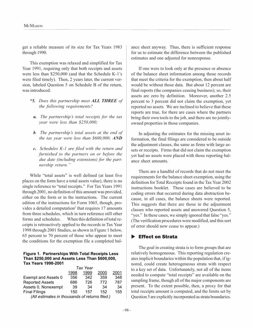
- 98 -
MCMAHON
get a reliable measure of its size for Tax Years 1983through 1990.
This exemption was relaxed and simplified for TaxYear 1991, requiring only that both receipts and assetswere less than $250,000 (and that the Schedule K-1�swere filed timely). Then, 2 years later, the current ver-sion, labeled Question 5 on Schedule B of the return,was introduced:
�5. Does this partnership meet ALL THREE ofthe following requirements?
a. The partnership�s total receipts for the taxyear were less than $250,000;
b. The partnership�s total assets at the end ofthe tax year were less than $600,000; AND
c. Schedules K-1 are filed with the return andfurnished to the partners on or before thedue date (including extensions) for the part-nership return.�
While �total assets� is well defined (at least fiveplaces on the form have a total assets value), there is nosingle reference to �total receipts.� For Tax Years 1991through 2001, no definition of this amount was provided,either on the form or in the instructions. The currentedition of the instructions for Form 1065, though, pro-vides a detailed computation2 that requires 17 amountsfrom three schedules, which in turn reference still otherforms and schedules. When this definition of total re-ceipts is retroactively applied to the records in Tax Year1998 through 2001 Studies, as shown in Figure 1 below,65 percent to 70 percent of those who appear to meetthe conditions for the exemption file a completed bal-
ance sheet anyway. Thus, there is sufficient responsefor us to estimate the difference between the publishedestimates and one adjusted for nonresponse.
If one were to look only at the presence or absenceof the balance sheet information among those recordsthat meet the criteria for the exemption, then about halfwould be without those data. But about 12 percent arefinal reports (the companies ceasing business); so, theirassets are zero by definition. Moreover, another 2.5percent to 3 percent did not claim the exemption, yetreported no assets. We are inclined to believe that thesereports are true, for there are cases where the partnersbring their own tools to the job, and there are no jointly-owned properties in those companies.
In adjusting the estimates for the missing asset in-formation, the final filings are considered to be outsidethe adjustment classes, the same as firms with large as-sets or receipts. Firms that did not claim the exemptionyet had no assets were placed with those reporting bal-ance sheet amounts.
There are a handful of records that do not meet therequirements for the balance sheet exemption, using thedefinition for Total Receipts found in the Tax Year 2002instructions booklet. These cases are believed to becoding errors that occurred during data abstraction be-cause, in all cases, the balance sheets were reported.This suggests that there are those in the adjustmentclasses who reported assets and answered Question 5,�yes.� In these cases, we simply ignored that false �yes.�(The verification procedures were modified, and this sortof error should now cease to appear.)
� Effect on Strata
The goal in creating strata is to form groups that arerelatively homogeneous. This reporting regulation cre-ates implicit boundaries within the population that, if ig-nored, could create heterogeneous strata with respectto a key set of data. Unfortunately, not all of the itemsneeded to compute �total receipts� are available on thesampling frame, though all of the major components arepresent. To the extent possible, then, a proxy for thattotal receipts amount is computed, and the limits set byQuestion 5 are explicitly incorporated as strata boundaries.
Figure 1. Partnerships With Total Receipts Less Than $250,000 and Assets Less Than $600,000, Tax Years 1998-2001 Tax Year 1998 1999 2000 2001 Exempt and Assets 0 356 342 359 348 Reported Assets 686 726 772 787 Assets 0, Nonexempt 39 34 34 34 Final Filings 150 157 152 155 (All estimates in thousands of returns filed.)
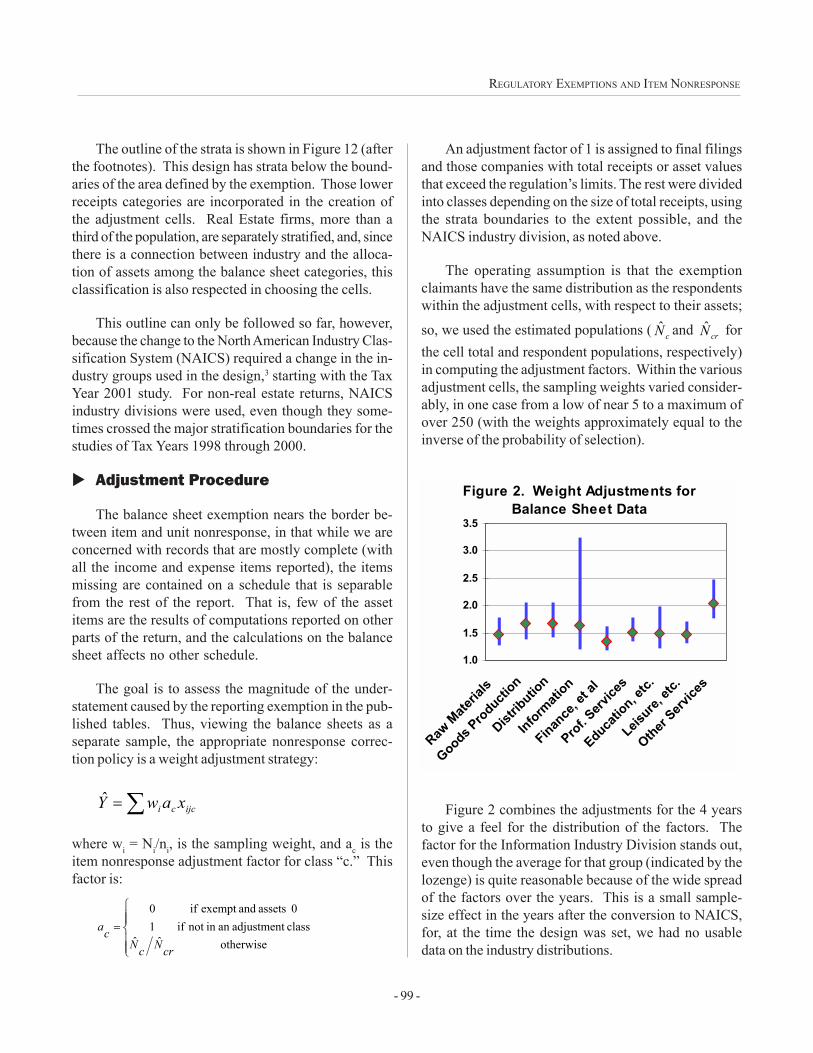
- 99 -
REGULATORY EXEMPTIONS AND ITEM NONRESPONSE
The outline of the strata is shown in Figure 12 (afterthe footnotes). This design has strata below the bound-aries of the area defined by the exemption. Those lowerreceipts categories are incorporated in the creation ofthe adjustment cells. Real Estate firms, more than athird of the population, are separately stratified, and, sincethere is a connection between industry and the alloca-tion of assets among the balance sheet categories, thisclassification is also respected in choosing the cells.
This outline can only be followed so far, however,because the change to the North American Industry Clas-sification System (NAICS) required a change in the in-dustry groups used in the design,3 starting with the TaxYear 2001 study. For non-real estate returns, NAICSindustry divisions were used, even though they some-times crossed the major stratification boundaries for thestudies of Tax Years 1998 through 2000.
� Adjustment Procedure
The balance sheet exemption nears the border be-tween item and unit nonresponse, in that while we areconcerned with records that are mostly complete (withall the income and expense items reported), the itemsmissing are contained on a schedule that is separablefrom the rest of the report. That is, few of the assetitems are the results of computations reported on otherparts of the return, and the calculations on the balancesheet affects no other schedule.
The goal is to assess the magnitude of the under-statement caused by the reporting exemption in the pub-lished tables. Thus, viewing the balance sheets as aseparate sample, the appropriate nonresponse correc-tion policy is a weight adjustment strategy:
ijcci xawY ���
where wi = Ni/ni, is the sampling weight, and ac is theitem nonresponse adjustment factor for class �c.� Thisfactor is:
otherwiseclass adjustmentan in not if0 assets andexempt if
��10
���
���
�
�
crNcNca
An adjustment factor of 1 is assigned to final filingsand those companies with total receipts or asset valuesthat exceed the regulation�s limits. The rest were dividedinto classes depending on the size of total receipts, usingthe strata boundaries to the extent possible, and theNAICS industry division, as noted above.
The operating assumption is that the exemptionclaimants have the same distribution as the respondentswithin the adjustment cells, with respect to their assets;
so, we used the estimated populations ( cN� and crN� forthe cell total and respondent populations, respectively)in computing the adjustment factors. Within the variousadjustment cells, the sampling weights varied consider-ably, in one case from a low of near 5 to a maximum ofover 250 (with the weights approximately equal to theinverse of the probability of selection).
Figure 2. Weight Adjustments for Balance Sheet Data
1.0
1.5
2.0
2.5
3.0
3.5
Raw M
ateria
ls
Goods Pro
duction
Distrib
ution
Informati
on
Finance
, et a
l
Prof. Serv
ices
Educatio
n, etc.
Leisure,
etc.
Other Serv
ices
Figure 2 combines the adjustments for the 4 yearsto give a feel for the distribution of the factors. Thefactor for the Information Industry Division stands out,even though the average for that group (indicated by thelozenge) is quite reasonable because of the wide spreadof the factors over the years. This is a small sample-size effect in the years after the conversion to NAICS,for, at the time the design was set, we had no usabledata on the industry distributions.
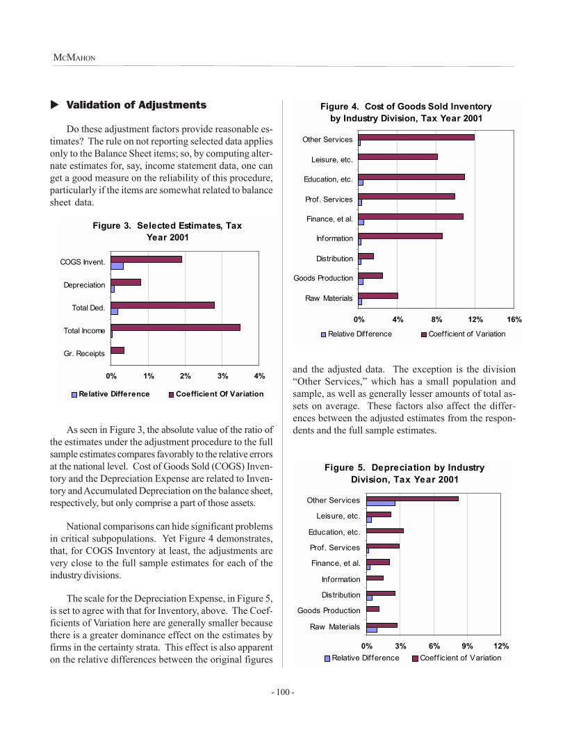
- 100 -
MCMAHON
� Validation of Adjustments
Do these adjustment factors provide reasonable es-timates? The rule on not reporting selected data appliesonly to the Balance Sheet items; so, by computing alter-nate estimates for, say, income statement data, one canget a good measure on the reliability of this procedure,particularly if the items are somewhat related to balancesheet data.
and the adjusted data. The exception is the division�Other Services,� which has a small population andsample, as well as generally lesser amounts of total as-sets on average. These factors also affect the differ-ences between the adjusted estimates from the respon-dents and the full sample estimates.
Figure 3. Selected Estimates, Tax Year 2001
0% 1% 2% 3% 4%
Gr. Receipts
Total Income
Total Ded.
Depreciation
COGS Invent.
Relative Difference Coefficient Of Variation
As seen in Figure 3, the absolute value of the ratio ofthe estimates under the adjustment procedure to the fullsample estimates compares favorably to the relative errorsat the national level. Cost of Goods Sold (COGS) Inven-tory and the Depreciation Expense are related to Inven-tory and Accumulated Depreciation on the balance sheet,respectively, but only comprise a part of those assets.
National comparisons can hide significant problemsin critical subpopulations. Yet Figure 4 demonstrates,that, for COGS Inventory at least, the adjustments arevery close to the full sample estimates for each of theindustry divisions.
The scale for the Depreciation Expense, in Figure 5,is set to agree with that for Inventory, above. The Coef-ficients of Variation here are generally smaller becausethere is a greater dominance effect on the estimates byfirms in the certainty strata. This effect is also apparenton the relative differences between the original figures
Figure 5. Depreciation by Industry Division, Tax Year 2001
0% 3% 6% 9% 12%
Raw Materials
Goods Production
Distribution
Information
Finance, et al.
Prof. Services
Education, etc.
Leisure, etc.
Other Services
Relative Dif ference Coeff icient of Variation
Figure 4. Cost of Goods Sold Inventory by Industry Division, Tax Year 2001
0% 4% 8% 12% 16%
Raw Materials
Goods Production
Distribution
Information
Finance, et al.
Prof. Services
Education, etc.
Leisure, etc.
Other Services
Relative Difference Coefficient of Variation
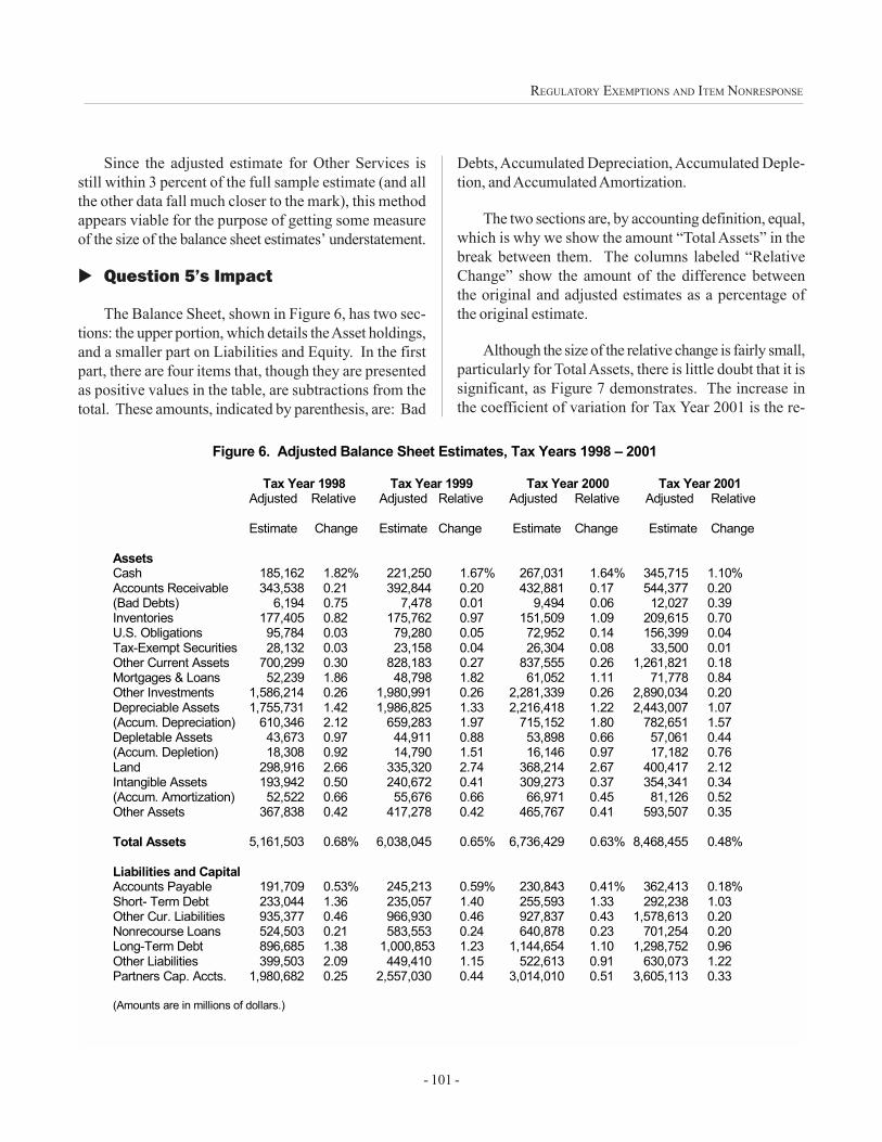
- 101 -
REGULATORY EXEMPTIONS AND ITEM NONRESPONSE
Since the adjusted estimate for Other Services isstill within 3 percent of the full sample estimate (and allthe other data fall much closer to the mark), this methodappears viable for the purpose of getting some measureof the size of the balance sheet estimates� understatement.
� Question 5�s Impact
The Balance Sheet, shown in Figure 6, has two sec-tions: the upper portion, which details the Asset holdings,and a smaller part on Liabilities and Equity. In the firstpart, there are four items that, though they are presentedas positive values in the table, are subtractions from thetotal. These amounts, indicated by parenthesis, are: Bad
Debts, Accumulated Depreciation, Accumulated Deple-tion, and Accumulated Amortization.
The two sections are, by accounting definition, equal,which is why we show the amount �Total Assets� in thebreak between them. The columns labeled �RelativeChange� show the amount of the difference betweenthe original and adjusted estimates as a percentage ofthe original estimate.
Although the size of the relative change is fairly small,particularly for Total Assets, there is little doubt that it issignificant, as Figure 7 demonstrates. The increase inthe coefficient of variation for Tax Year 2001 is the re-
Figure 6. Adjusted Balance Sheet Estimates, Tax Years 1998 � 2001 Tax Year 1998 Tax Year 1999 Tax Year 2000 Tax Year 2001 Adjusted Relative Adjusted Relative Adjusted Relative Adjusted Relative Estimate Change Estimate Change Estimate Change Estimate Change Assets Cash 185,162 1.82% 221,250 1.67% 267,031 1.64% 345,715 1.10% Accounts Receivable 343,538 0.21 392,844 0.20 432,881 0.17 544,377 0.20 (Bad Debts) 6,194 0.75 7,478 0.01 9,494 0.06 12,027 0.39 Inventories 177,405 0.82 175,762 0.97 151,509 1.09 209,615 0.70 U.S. Obligations 95,784 0.03 79,280 0.05 72,952 0.14 156,399 0.04 Tax-Exempt Securities 28,132 0.03 23,158 0.04 26,304 0.08 33,500 0.01 Other Current Assets 700,299 0.30 828,183 0.27 837,555 0.26 1,261,821 0.18 Mortgages & Loans 52,239 1.86 48,798 1.82 61,052 1.11 71,778 0.84 Other Investments 1,586,214 0.26 1,980,991 0.26 2,281,339 0.26 2,890,034 0.20 Depreciable Assets 1,755,731 1.42 1,986,825 1.33 2,216,418 1.22 2,443,007 1.07 (Accum. Depreciation) 610,346 2.12 659,283 1.97 715,152 1.80 782,651 1.57 Depletable Assets 43,673 0.97 44,911 0.88 53,898 0.66 57,061 0.44 (Accum. Depletion) 18,308 0.92 14,790 1.51 16,146 0.97 17,182 0.76 Land 298,916 2.66 335,320 2.74 368,214 2.67 400,417 2.12 Intangible Assets 193,942 0.50 240,672 0.41 309,273 0.37 354,341 0.34 (Accum. Amortization) 52,522 0.66 55,676 0.66 66,971 0.45 81,126 0.52 Other Assets 367,838 0.42 417,278 0.42 465,767 0.41 593,507 0.35 Total Assets 5,161,503 0.68% 6,038,045 0.65% 6,736,429 0.63% 8,468,455 0.48% Liabilities and Capital Accounts Payable 191,709 0.53% 245,213 0.59% 230,843 0.41% 362,413 0.18% Short- Term Debt 233,044 1.36 235,057 1.40 255,593 1.33 292,238 1.03 Other Cur. Liabilities 935,377 0.46 966,930 0.46 927,837 0.43 1,578,613 0.20 Nonrecourse Loans 524,503 0.21 583,553 0.24 640,878 0.23 701,254 0.20 Long-Term Debt 896,685 1.38 1,000,853 1.23 1,144,654 1.10 1,298,752 0.96 Other Liabilities 399,503 2.09 449,410 1.15 522,613 0.91 630,073 1.22 Partners Cap. Accts. 1,980,682 0.25 2,557,030 0.44 3,014,010 0.51 3,605,113 0.33 (Amounts are in millions of dollars.)
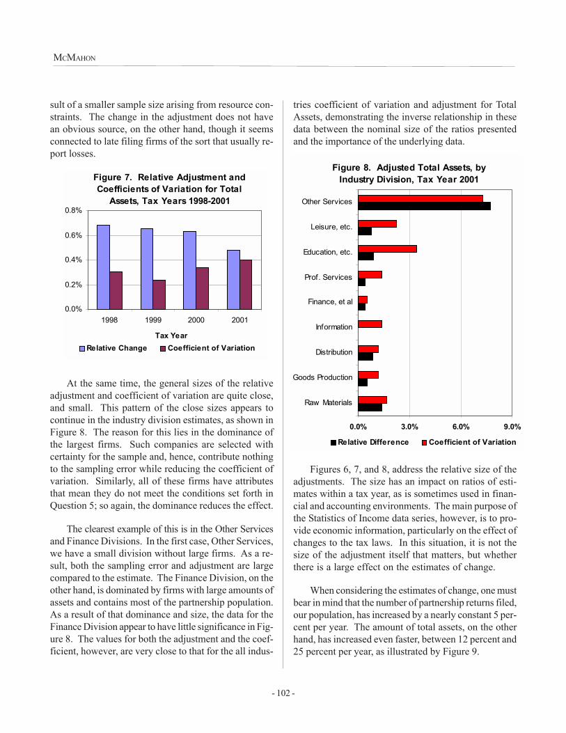
- 102 -
MCMAHON
sult of a smaller sample size arising from resource con-straints. The change in the adjustment does not havean obvious source, on the other hand, though it seemsconnected to late filing firms of the sort that usually re-port losses.
tries coefficient of variation and adjustment for TotalAssets, demonstrating the inverse relationship in thesedata between the nominal size of the ratios presentedand the importance of the underlying data.
Figure 7. Relative Adjustment and Coefficients of Variation for Total
Assets, Tax Years 1998-2001
0.0%
0.2%
0.4%
0.6%
0.8%
1998 1999 2000 2001
Tax YearRelative Change Coefficient of Variation
At the same time, the general sizes of the relativeadjustment and coefficient of variation are quite close,and small. This pattern of the close sizes appears tocontinue in the industry division estimates, as shown inFigure 8. The reason for this lies in the dominance ofthe largest firms. Such companies are selected withcertainty for the sample and, hence, contribute nothingto the sampling error while reducing the coefficient ofvariation. Similarly, all of these firms have attributesthat mean they do not meet the conditions set forth inQuestion 5; so again, the dominance reduces the effect.
The clearest example of this is in the Other Servicesand Finance Divisions. In the first case, Other Services,we have a small division without large firms. As a re-sult, both the sampling error and adjustment are largecompared to the estimate. The Finance Division, on theother hand, is dominated by firms with large amounts ofassets and contains most of the partnership population.As a result of that dominance and size, the data for theFinance Division appear to have little significance in Fig-ure 8. The values for both the adjustment and the coef-ficient, however, are very close to that for the all indus-
Figures 6, 7, and 8, address the relative size of theadjustments. The size has an impact on ratios of esti-mates within a tax year, as is sometimes used in finan-cial and accounting environments. The main purpose ofthe Statistics of Income data series, however, is to pro-vide economic information, particularly on the effect ofchanges to the tax laws. In this situation, it is not thesize of the adjustment itself that matters, but whetherthere is a large effect on the estimates of change.
When considering the estimates of change, one mustbear in mind that the number of partnership returns filed,our population, has increased by a nearly constant 5 per-cent per year. The amount of total assets, on the otherhand, has increased even faster, between 12 percent and25 percent per year, as illustrated by Figure 9.
Figure 8. Adjusted Total Assets, by Industry Division, Tax Year 2001
0.0% 3.0% 6.0% 9.0%
Raw Materials
Goods Production
Distribution
Information
Finance, et al
Prof. Services
Education, etc.
Leisure, etc.
Other Services
Relative Difference Coefficient of Variation
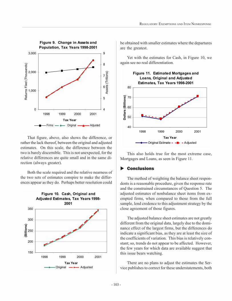
- 103 -
REGULATORY EXEMPTIONS AND ITEM NONRESPONSE
That figure, above, also shows the difference, orrather the lack thereof, between the original and adjustedestimates. On this scale, the difference between thetwo is barely discernible. This is not unexpected, for therelative differences are quite small and in the same di-rection (always greater).
Both the scale required and the relative nearness ofthe two sets of estimates conspire to make the differ-ences appear as they do. Perhaps better resolution could
be obtained with smaller estimates where the departuresare the greatest.
Yet with the estimates for Cash, in Figure 10, weagain see no real differentiation.
Figure 9. Change in Assets and Population, Tax Years 1998-2001
0
1,000
2,000
3,000
1998 1999 2000 2001
Tax Year
Ret
urns
File
d (T
hous
ands
)
4
5
6
7
8
9
Asse
ts (T
rillio
ns)
Firms Original Adjusted
Figure 10. Cash, Original and Adjusted Estimates, Tax Years 1998-
2001
150
200
250
300
350
1998 1999 2000 2001
Tax Year
(Bill
ions
)
Original Adjusted
This also holds true for the most extreme case,Mortgages and Loans, as seen in Figure 11.
� Conclusions
The method of weighting the balance sheet respon-dents is a reasonable procedure, given the response rateand the constrained circumstances of Question 5. Theadjusted estimates of nonbalance sheet items from ex-empted firms, when compared to those from the fullsample, lend credence to this adjustment strategy by theclose agreement of those figures.
The adjusted balance sheet estimates are not greatlydifferent from the original data, largely due to the domi-nance effect of the largest firms, but the differences doindicate a significant bias, as they are at least the size ofthe coefficients of variation. This bias is relatively con-stant; so, trends do not appear to be affected. However,the few years for which data are available suggest thatthis issue bears watching.
There are no plans to adjust the estimates the Ser-vice publishes to correct for these understatements, both
Figure 11. Estimated Mortgages and Loans, Original and Adjusted
Estimates, Tax Years 1998-2001
40
50
60
70
80
1998 1999 2000 2001
Tax Year
Dol
lars
(Bill
ions
)
Original Estimate Adjusted
- 104 -
MCMAHON
because the adjustment amounts for each item appearto be reasonably constant, and because the uncorrectedtotals provide a benchmark to external users of the datawho review estimates from either the Office of TaxAnalysis or the Joint Committee.
Nevertheless, we are considering adding a table tothe annual publication comparing the full sample esti-mates to the adjusted results, mostly for the use of thoseresearchers who focus on investment type ratios.
It is clear that, while the administrative systems doprovide a very good source for population data, one hasto be cautious about the existence of filing rules that canaffect both sample designs and subsequent analysis.
� Footnotes
1 Internal Revenue Service, Statistics of IncomeBulletin, Fall 2002 (or other Fall editions), Wash-ington, DC.
2 Total receipts is the sum of:
Form 1065, pg .1: Gross Receipts, Ordinary In-come From Other Partnerships, Net Farm Profit,Net Gain or Loss From the Sale of Business Prop-erty, and Other Income;
Schedule K: Non Real Estate Rents, Interest In-come, Ordinary Dividends, Royalty Income, ShortTerm Capital Gains, Long Term Capital Gains (Taxedat the 28 Percent Rate), Other Portfolio Income,Income Under Section 1231, and Other Income;
Form 8825: Gross Real Estate Rents, Net Gainor Loss From the Sale of Business Property, andIncome From Other Real Estate Partnerships.
3 McMahon, Paul (2000), �Changing Industry CodeSystems: The Impact on the Statistics of IncomePartnership Studies,� Proceedings of the SecondInternational Conference on EstablishmentSurveys, American Statistical Association.
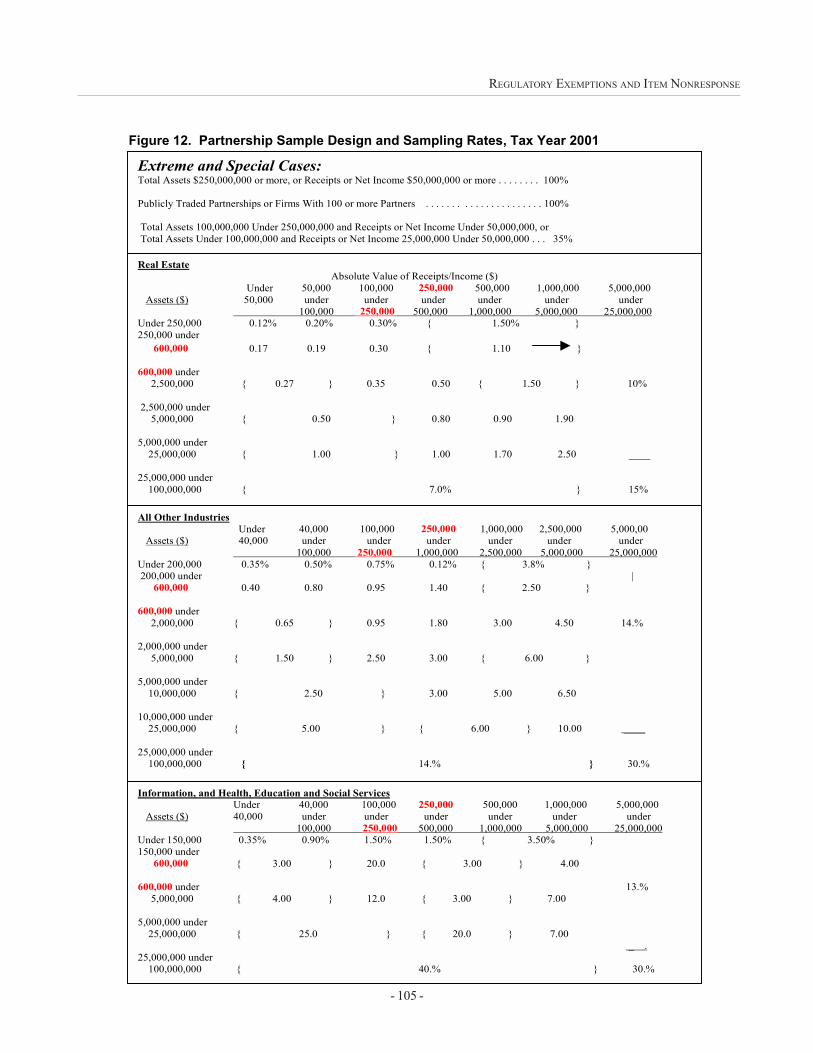
- 105 -
REGULATORY EXEMPTIONS AND ITEM NONRESPONSE
Figure 12. Partnership Sample Design and Sampling Rates, Tax Year 2001
Extreme and Special Cases: Total Assets $250,000,000 or more, or Receipts or Net Income $50,000,000 or more . . . . . . . . 100% Publicly Traded Partnerships or Firms With 100 or more Partners . . . . . . . . . . . . . . . . . . . . . . 100% Total Assets 100,000,000 Under 250,000,000 and Receipts or Net Income Under 50,000,000, or Total Assets Under 100,000,000 and Receipts or Net Income 25,000,000 Under 50,000,000 . . . 35%
Real Estate Absolute Value of Receipts/Income ($)
Under 50,000 100,000 250,000 500,000 1,000,000 5,000,000 Assets ($) 50,000 under under under under under under
100,000 250,000 500,000 1,000,000 5,000,000 25,000,000 Under 250,000 0.12% 0.20% 0.30% { 1.50% } 250,000 under 600,000 0.17 0.19 0.30 { 1.10 } 600,000 under 2,500,000 { 0.27 } 0.35 0.50 { 1.50 } 10% 2,500,000 under 5,000,000 { 0.50 } 0.80 0.90 1.90 5,000,000 under 25,000,000 { 1.00 } 1.00 1.70 2.50 ____ 25,000,000 under 100,000,000 { 7.0% } 15%
All Other Industries Under 40,000 100,000 250,000 1,000,000 2,500,000 5,000,00 Assets ($) 40,000 under under under under under under
100,000 250,000 1,000,000 2,500,000 5,000,000 25,000,000 Under 200,000 0.35% 0.50% 0.75% 0.12% { 3.8% } 200,000 under | 600,000 0.40 0.80 0.95 1.40 { 2.50 } 600,000 under 2,000,000 { 0.65 } 0.95 1.80 3.00 4.50 14.% 2,000,000 under 5,000,000 { 1.50 } 2.50 3.00 { 6.00 } 5,000,000 under 10,000,000 { 2.50 } 3.00 5.00 6.50 10,000,000 under 25,000,000 { 5.00 } { 6.00 } 10.00 ____ 25,000,000 under 100,000,000 { 14.% } 30.%
Information, and Health, Education and Social Services Under 40,000 100,000 250,000 500,000 1,000,000 5,000,000
Assets ($) 40,000 under under under under under under 100,000 250,000 500,000 1,000,000 5,000,000 25,000,000
Under 150,000 0.35% 0.90% 1.50% 1.50% { 3.50% } 150,000 under 600,000 { 3.00 } 20.0 { 3.00 } 4.00 600,000 under 13.% 5,000,000 { 4.00 } 12.0 { 3.00 } 7.00 5,000,000 under 25,000,000 { 25.0 } { 20.0 } 7.00 _ . 25,000,000 under 100,000,000 { 40.% } 30.%
- 107 -
Indexof IRS Methodology Reports
on Statistical Uses of Administrative Records
Special Studies in Federal Tax Statistics--2002Selected papers given primarily at the 2002 Annual Meetings of the American Statistical Association in New YorkCity and at the 2002 National Tax Association Conference in Orlando, FL. The volume is divided into seven majorsections. It begins with two papers on recent IRS research. Section 2 includes a group of four papers on method-ological and analytical advances in tax statistics. Section 3 presents two papers on statistical uses of administrativerecords. Section 4 contains a paper on disseminating IRS locality data. Section 5 includes a paper on confidentialityand data access issues. Section 6 presents a paper on measuring the quality of IRS responses to taxpayer inquiries.Finally, Section 7 includes two papers on distributional theory and computation.
Special Studies in Federal Tax Statistics--2000-2001Selected papers given primarily at the 2000 and 2001 Annual Meetings of the American Statistical Association inIndianapolis, Indiana and Atlanta, Georgia, plus one other paper presented at the International Conference on Estab-lishment Surveys II in Buffalo, New York in 2000. The volume is divided into four major sections. The book beginswith five papers on statistical applications. Section 2 presents two papers on confidentiality and data access issues.Section 3 presents two papers on changing industry codes. Finally, Section 4 includes five papers on analyses ofFederal tax and information returns.
Turning Administrative Systems Into Information Systems--1999Selected papers given at the 1999 Annual Meetings of the American Statistical Association (ASA) in Baltimore, MD.In addition, the report includes one paper presented at the 1998 ASA conference in Dallas, TX. The volume is dividedinto six major sections. The book begins with a complete ASA session analyzing administrative records from the U.S.tax system. It contains four papers, as well as a set of comments on the presentations. Section 2 presents fourpapers on the statistical uses of administrative records. Section 3 includes two papers, which focus on employeesatisfaction and customer satisfaction surveys at the IRS. Section 4 contains two papers, one of which was pre-sented at the 1998 ASA conference, that provide an update on the Survey of Consumer Finances. Section 5 presentsone paper that looks at the feasibility of preparing State corporate data by matching receipts and employment data byState and industry. Finally, the volume concludes with a paper on distributional theory and computation.
Turning Administrative Systems Into Information Systems--1998-1999Selected papers given at the 1998 Annual Meetings of the American Statistical Association in Dallas, Texas. Inaddition, the report includes a session of papers presented in 1999 at the Annual Meetings of the American Eco-nomic Association (AEA) plus one other paper. The volume is divided into five major sections. The book begins withthe AEA session in memory of the late Dr. Daniel B. Radner, Social Security Administration economist. It containsfour papers on new empirical findings in the distributions of personal income and wealth, as well as two sets ofintroductory remarks and two sets of comments on the presentations. Section 2 presents two papers on data mea-surement and data bases for economic research. Section 3 includes two papers, which focus on sample design,estimation, and imputation research. Section 4 explores issues dealing with public-use files, including the potential fordisclosure. Finally, Section 5 concludes the volume with a paper verifying the classification of public charities in the1994 Statistics of Income Study Sample. (It is the only paper not presented at the ASA or AEA meetings.)

- 108 -
INDEX
Turning Administrative Systems Into Information Systems--1996-1997Selected papers given primarily at the 1996 and 1997 Annual Meetings of the American Statistical Association inChicago, Illinois and Anaheim, California, plus one non-ASA article. The volume is divided into nine major sections.The book begins with a paper originally printed as a textbook article on inheritance and wealth in America. Section 2presents papers on using administrative records for generating national statistics. Section 3 contains two sets of panelreports on the statistical uses of administrative records. Section 4 focuses on methodological research. Section 5explores issues dealing with quality improvement in government. Section 6 presents a panel discussion on CustomerSatisfaction Surveys. Section 7 focuses on the effect of downsizing on Federal statistics. Section 8 explores theprivacy area. Finally, Section 9 concludes with seven papers on statistical disclosure limitation.
Turning Administrative Systems Into Information Systems--1995Selected papers given primarily at the 1995 Annual Meetings of the American Statistical Association in Orlando,Florida and another conference. The volume is divided into five major sections. The book begins with a paper on SOImigration data, giving an example of how this unique dataset can be used by demographers and policy researchers.Section 2 presents papers on sample designs and redesigns, as well as on SOI efforts in the corporation and partner-ship areas. Section 3 contains papers on weighting and estimation research. Section 4 focuses on analytical ap-proaches to quality improvement, from graphical techniques to cognitive research. Finally, Section 5 concludes withpapers from an invited session on record linkage applications for health care policy, a session organized by SOI inview of its long-term interest in improving matching techniques for administrative and survey data.
Turning Administrative Systems Into Information Systems--1994Selected papers given primarily at the 1994 Annual Meetings of the American Statistical Association in Toronto,Ontario, Canada. The volume is divided into nine major sections. The book begins with an overview of the Statisticsof Income Programs, describing the origins and customers of various SOI data and highlighting our products andservices. Section 2 presents the descriptive results from two recent studies--one on sales of capital assets and one onself-employed nonfilers. Section 3 contains papers and discussion from a session on privacy issues involved in usingadministrative record data. The next two sections are much more methodical in nature: Section 4 focuses on sampledesign and estimation work in SOI, beginning with a reprint of a 1963 paper by W. Edwards Deming, which presentsan evaluation of the SOI sample. Section 5 presents data on record linkage. Section 6 draws together the papersfrom a session on nonresponse in Federal surveys. Section 7 is a more statistical section, which contains a collectionof papers on imputation methodology in a number of different arenas. Section 8 focuses on another long-time themeof these volumes--quality improvement efforts. Finally, Section 9 presents two unrelated papers on data preparationtechniques.
Turning Administrative Systems Into Information Systems--1993Selected papers given at the 1993 Annual Meetings of the American Statistical Association in San Francisco, Califor-nia and other related conferences. The volume contains seven major sections, each focusing on a somewhat differ-ent area of research. The first section begins with a paper that presents a view for the future of the Federal statisticalsystem. This effort is part of a dialogue with other agency leaders to redefine a cohesive plan for Federal dataproducers and users. Section 2 contains several descriptive papers based on tax data about individuals, and Section 3looks at similar uses of tax data for businesses. Section 4 focuses on sample design issues for several SOI projects, whileSection 5 presents information on improvements to analytical techniques. Finally, Sections 6 and 7 describe a number ofdifferent studies SOI is involved in to improve the quality and productivity of other areas of IRS.
Turning Administrative Systems Into Information Systems--1991-1992Selected papers given mostly at the 1991 and 1992 Annual meetings of the American Statistical Association, held,respectively, in Atlanta, Georgia and Boston, Massachusetts. Papers chosen for this volume exemplify some of the

- 109 -
INDEX
basic changes that are occurring in the Statistics of Income program during the 1990’s, including discussions ofmethodological improvements and applications currently under way in the U.S. Federal statistical community. Thevolume contains seven general areas of interest: information from tax return data; the 1989 Survey of ConsumerFinances; estimation and methodological research in the SOI business program; sample design and weighting issuesin the SOI individual program; some quality improvement applications; some technological innovations for SOIresearch; and a look to the future data needs for the Federal sector. Previous volumes in the series were calledStatistics of Income and Related Administrative Record Research (see below). The title was changed to more clearlyreflect how the Internal Revenue Service’s Statistics of Income function is adapting to better meet the informationalneeds of its many customers.
Statistics of Income and Related Administrative Record Research--1990Selected papers given primarily at the 1990 Annual meeting of the American Statistical Association in Anaheim,California. Papers selected for this volume contain discussions of methodological improvements and applicationscurrently under way in the U.S. Federal statistical community. In particular, the focus is on work being done by theStatistics of Income Division of the Internal Revenue Service (IRS). The volume covers five general areas: longi-tudinal panel data and estimation issues; analytical research using survey and administrative data; design issues forFederal surveys; information on the conclusions of the Establishment Reporting Unit Match Study; and a look atfuture data needs for the Federal sector.
Statistics of Income and Related Administrative Record Research--1988-1989Selected papers given mostly at the 1988 and 1989 Annual Meetings of the American Statistical Association in NewOrleans, Louisiana and Washington, D.C., respectively. Papers for the volume focus on perspectives on statistics ingovernment--in celebration of ASA’s 150th anniversary; improvements in income and wealth estimation; method-ological enhancements to administrative record data; some looks at the effects of tax reform; and technologicalinnovations for statistical use.
Statistics of Income and Related Administrative Record Research--1986-1987Selected papers given, for the most part, at the 1986 and 1987 Annual Meetings of American Statistical Associationin Chicago and San Francisco, respectively. Papers focus on ongoing wealth estimation research and U.S. andCanadian efforts regarding methodological enhancements to corporate and individual tax data and recent refine-ments to disclosure avoidance techniques.
Record Linkage Techniques--1985*The Proceedings of the Workshop on Exact Matching Methodologies held in Arlington, Virginia, May 9-10, 1985.Includes landmark background papers on record linkage use and papers describing methodological enhancements,applications, and technological developments, as well as extensive bibliographic material on exact matching.
Statistical Uses of Administrative Records: Recent Research and Present Prospects*A two-volume reference handbook on research results involving the use of administrative records for statisticalpurposes from 1979 through 1982:
� Volume I (March 1984) focuses on general considerations in administrative record research, applicationsof income tax data, uses based on data from other major administrative record systems, and enhancementsto statistical systems using administrative data.
- 110 -
INDEX
� Volume II (July 1984) focuses on comparability and quality issues, access to administrative records forstatistical purposes, selected examples of end uses of linked administrative statistical systems, and a statusreport that sets goals for the future.
Statistics of Income and Related Administrative Record Research--1984*Selected papers given at the 1984 Annual Meeting of American Statistical Association in Philadelphia. Papers focuson future policy issues, applications, exact matching techniques, quality control, missing data, and sample de-sign issues.
Statistics of Income and Related Administrative Record Research--1983*Selected papers given at the 1983 Annual Meeting of American Statistical Association in Toronto. Papers focus onuse of administrative records in censuses and surveys, applications for epidemiologic research and other statisticalpurposes, and statistical techniques involving imputation and disclosure and confidentiality
Statistics of Income and Related Administrative Record Research--1982*Selected papers given at the 1982 Annual Meeting of American Statistical Association in Cincinnati. Papers focuson statistical uses of administrative records, resulting methodologic advances, and estimates and projections forintercensal updates.
Statistics of Income and Related Administrative Record Research*Selected papers given at the 1981 Annual Meeting of American Statistical Association in Detroit. Papers focus onapplications and methodologies with an emphasis on IRS’s Statistics of Income Program, the Small Business DataBase, nonprofit and pension data, and on Canada’s Generalized Iterative Record Linkage System.
Economic and Demographic Statistics*Selected papers given at the 1980 Annual Meeting of American Statistical Association in Houston. Papers focus onevaluation of the 1977 Economic Census, CPS hot deck techniques, and efforts to upgrade Social Security’s Con-tinuous Work History Sample.
______________________________
*Out of print--Copies of selected papers can be obtained upon request.
NOTE: The IRS Methodology Reports on statistical uses of administrative records are now being offered free ofcharge. To obtain copies, write to:
Statistical Information Services (SIS)Statistics of Income Division (RAS:S:SS:SD)Internal Revenue ServiceP.O. Box 2608Washington, DC 20013-2608Phone: (202) 874-0410FAX: (202) 874-0964E-mail: [email protected]