SPECIAL FEATURE: PERSPECTIVE

The Inter-Sectoral Impact ModelIntercomparison Project (ISI–MIP):Project frameworkLila Warszawski, Katja Frieler1, Veronika Huber, Franziska Piontek, Olivia Serdeczny, and Jacob SchewePotsdam Institute for Climate Impact Research, 14412 Potsdam, Germany

Edited by Hans Joachim Schellnhuber, Potsdam Institute for Climate Impact Research, Potsdam, Germany, and approved September 4, 2013 (received for review July 3, 2013)

The Inter-Sectoral Impact Model Intercomparison Project offers a framework to compare climate impact projections in different sectors and atdifferent scales. Consistent climate and socio-economic input data provide the basis for a cross-sectoral integration of impact projections. Theproject is designed to enable quantitative synthesis of climate change impacts at different levels of global warming.This report briefly outlinesthe objectives and framework of the first, fast-tracked phase of Inter-Sectoral Impact Model Intercomparison Project, based on global impactmodels, and provides an overview of the participating models, input data, and scenario set-up.

multi-sector | climate data

The Inter-Sectoral Impact Model Intercom-parison Project (ISI-MIP) fast track tookplace between January 2012 and January2013, and was unique in bringing together28 global impact models from five differentsectors (Table 1). During this phase, a com-mon modeling protocol was designed, sim-ulations were performed, and the resultingsimulation data were collected in a centralarchive. Based on these data, an initial roundof analysis was carried out, the key outcomesof which are assembled in this special issue ofPNAS. The fast-track simulation data willbe made freely available for further analysisby the wider research community.The ISI-MIP fast track pursued several

specific goals: (i) a quantitative assessmentof global climate change impacts at differentlevels of global warming in a consistent set-ting across multiple sectors; (ii) basic uncer-tainty estimates based on the quantificationof intermodel variations for both general cir-culation models (GCMs) and global impactmodels; and (iii) to initiate an ongoing co-ordinated impact modeling improvementand intercomparison program, as well asan impact assessment effort driven by theentire community.The central motivation for the project can

be summarized by the question: What is thedifference between a 2 °C, 3 °C, and 4°Cwarmer world, and how well can we differ-entiate between them?The project builds on earlier climate

change risk assessments at the global scale,such as the UK Fast Track project (1), theClimate Impact Response Functions (2)initiative, and the more recent investiga-tion by Arnell et al. (3) covering climate

impacts in six sectors (water availability,river flooding, coastal flooding, agriculture,ecosystems, and energy demands) using acoherent set of climatic and socioeconomicscenarios. However, all existing cross-sectoral impact studies use only one im-pact model per sector, and are thus unableto formally assess uncertainties beyond thosestemming from climatic and socio-eco-nomic input data.In contrast, there are sector-specific multi-

impact-model studies, such as Cramer et al.(4) and Sitch et al. (5) in the biomes sector,WaterMIP (6) in the water sector, andAgMIP (7) in the agriculture sector. In thiscontext, ISI-MIP is intended to address thelack of a cross-sectoral multimodel assess-ment of impacts of climate change.The project serves the dual purpose of

facilitating process understanding and modeldevelopment in the scientific community,as well as providing quantitative resultsthat are readily available to stakeholdersand society in general. The timeline of thefast track was designed to deliver a firstset of results in time for assessment bythe Intergovernmental Panel on ClimateChange in preparation for the fifth assess-ment report. To further the above goalsbeyond this narrow timeline, a second,longer-term phase of ISI-MIP was initiatedin May 2013. This second phase is plannedto incorporate regional models, as well asadditional sectors and systems, enablingboth a cross-sectoral and cross-scale syn-thesis of the impacts of climate change.More information on the project can befound at www.isi-mip.org, including thedetailed fast-track modeling protocol.

Impact ModelsGlobal impact models from five differentsectors were involved in the ISI-MIP fasttrack (Table 1) (water, agriculture, biomes,coastal infrastructure, and malaria) as anexample of health impacts. In the case ofagriculture and water, existing intercompar-ison efforts AgMIP (7) and WaterMIP (6),respectively, ensured that much of the nec-essary simulation framework was already inplace. The agricultural component of ISI-MIP was coordinated under the umbrellaof AgMIP, and an ISI-MIP componentwas included in the AgMIP agro-economicmodel intercomparison (comprising themodels listed in Table 2).Each impact model was driven by a com-

mon daily, gridded climate dataset and de-livered results in the form of a sector-specificset of common output variables at time res-olutions ranging from subdaily to monthly.Harmonization across models was limited tothe driving climate input data and, whereapplicable, socio-economic data (populationand gross domestic product, GDP). Addi-tional input data were selected according tothe default settings of each model, to gain arepresentative picture of uncertainty acrossthe models using native settings. Furthersector-specific details can be found in thisspecial issue.

Author contributions: L.W., K.F., V.H., F.P., O.S., and J.S. designed

and wrote the paper.

The authors declare no conflict of interest.

This article is a PNAS Direct Submission.

1To whom correspondence should be addressed. E-mail: katja.frieler@pik-potsdam.de.

3228–3232 | PNAS | March 4, 2014 | vol. 111 | no. 9 www.pnas.org/cgi/doi/10.1073/pnas.1312330110

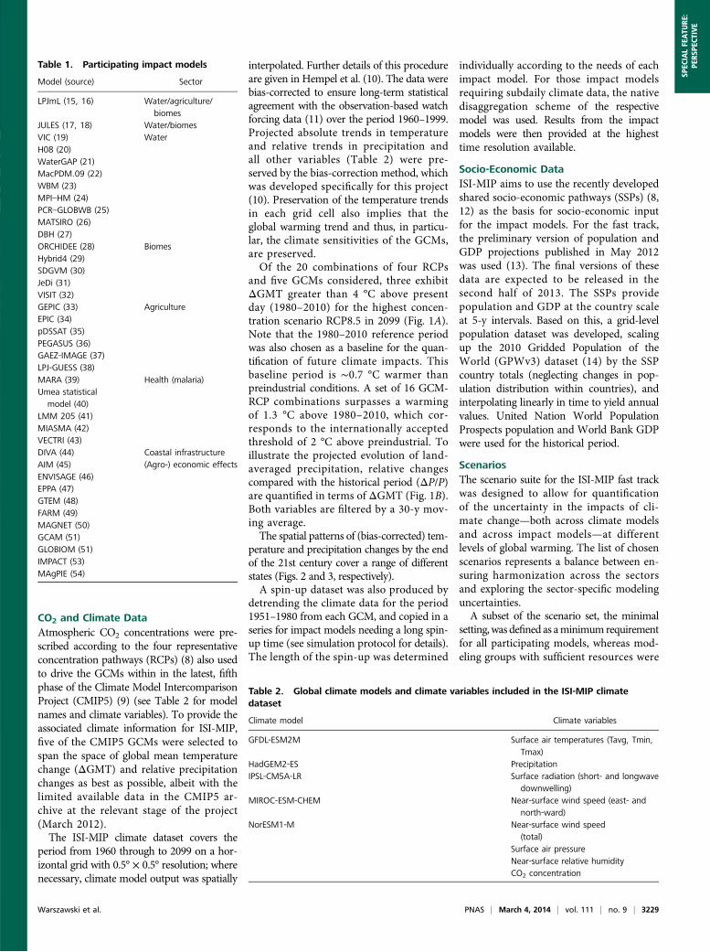
CO2 and Climate DataAtmospheric CO2 concentrations were pre-scribed according to the four representativeconcentration pathways (RCPs) (8) also usedto drive the GCMs within in the latest, fifthphase of the Climate Model IntercomparisonProject (CMIP5) (9) (see Table 2 for modelnames and climate variables). To provide theassociated climate information for ISI-MIP,five of the CMIP5 GCMs were selected tospan the space of global mean temperaturechange (ΔGMT) and relative precipitationchanges as best as possible, albeit with thelimited available data in the CMIP5 ar-chive at the relevant stage of the project(March 2012).The ISI-MIP climate dataset covers the

period from 1960 through to 2099 on a hor-izontal grid with 0.5° × 0.5° resolution; wherenecessary, climate model output was spatially

interpolated. Further details of this procedureare given in Hempel et al. (10). The data werebias-corrected to ensure long-term statisticalagreement with the observation-based watchforcing data (11) over the period 1960–1999.Projected absolute trends in temperatureand relative trends in precipitation andall other variables (Table 2) were pre-served by the bias-correction method, whichwas developed specifically for this project(10). Preservation of the temperature trendsin each grid cell also implies that theglobal warming trend and thus, in particu-lar, the climate sensitivities of the GCMs,are preserved.Of the 20 combinations of four RCPs

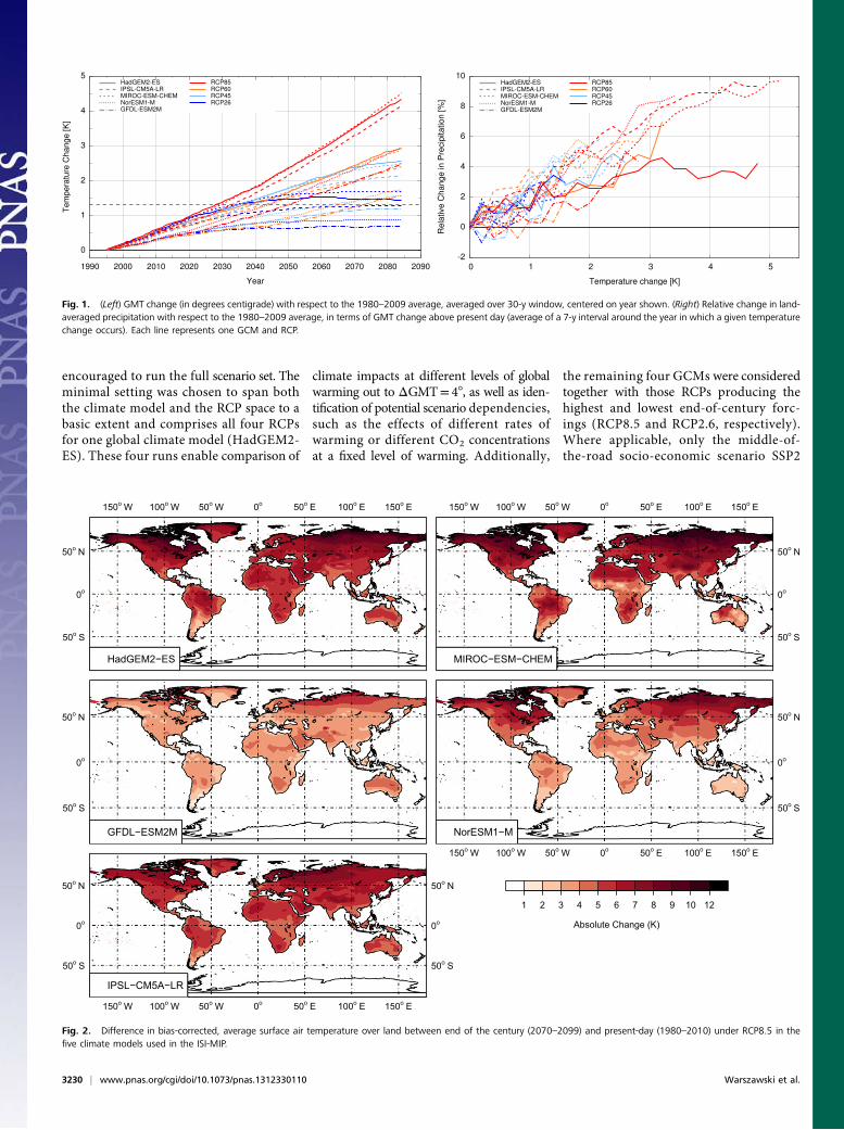
and five GCMs considered, three exhibitΔGMT greater than 4 °C above presentday (1980–2010) for the highest concen-tration scenario RCP8.5 in 2099 (Fig. 1A).Note that the 1980–2010 reference periodwas also chosen as a baseline for the quan-tification of future climate impacts. Thisbaseline period is ∼0.7 °C warmer thanpreindustrial conditions. A set of 16 GCM-RCP combinations surpasses a warmingof 1.3 °C above 1980–2010, which cor-responds to the internationally acceptedthreshold of 2 °C above preindustrial. Toillustrate the projected evolution of land-averaged precipitation, relative changescompared with the historical period (ΔP/P)are quantified in terms of ΔGMT (Fig. 1B).Both variables are filtered by a 30-y mov-ing average.The spatial patterns of (bias-corrected) tem-

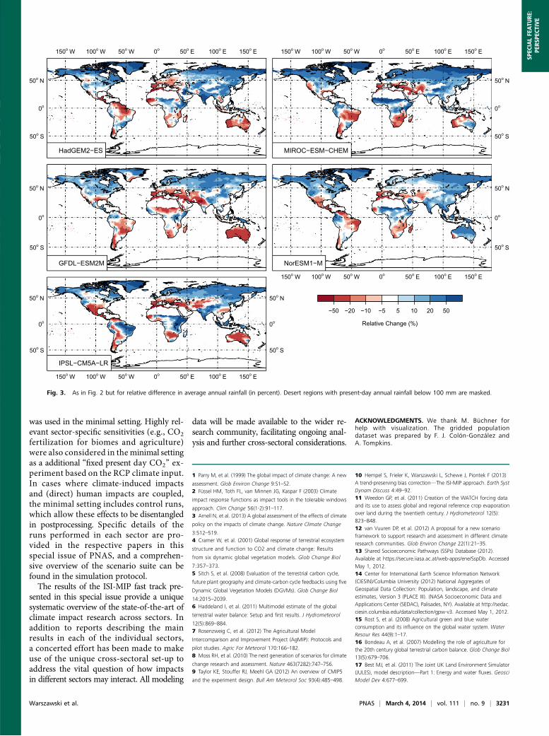
perature and precipitation changes by the endof the 21st century cover a range of differentstates (Figs. 2 and 3, respectively).A spin-up dataset was also produced by

detrending the climate data for the period1951–1980 from each GCM, and copied in aseries for impact models needing a long spin-up time (see simulation protocol for details).The length of the spin-up was determined

individually according to the needs of eachimpact model. For those impact modelsrequiring subdaily climate data, the nativedisaggregation scheme of the respectivemodel was used. Results from the impactmodels were then provided at the highesttime resolution available.

Socio-Economic DataISI-MIP aims to use the recently developedshared socio-economic pathways (SSPs) (8,12) as the basis for socio-economic inputfor the impact models. For the fast track,the preliminary version of population andGDP projections published in May 2012was used (13). The final versions of thesedata are expected to be released in thesecond half of 2013. The SSPs providepopulation and GDP at the country scaleat 5-y intervals. Based on this, a grid-levelpopulation dataset was developed, scalingup the 2010 Gridded Population of theWorld (GPWv3) dataset (14) by the SSPcountry totals (neglecting changes in pop-ulation distribution within countries), andinterpolating linearly in time to yield annualvalues. United Nation World PopulationProspects population and World Bank GDPwere used for the historical period.

ScenariosThe scenario suite for the ISI-MIP fast trackwas designed to allow for quantificationof the uncertainty in the impacts of cli-mate change—both across climate modelsand across impact models—at differentlevels of global warming. The list of chosenscenarios represents a balance between en-suring harmonization across the sectorsand exploring the sector-specific modelinguncertainties.A subset of the scenario set, the minimal

setting,was defined as aminimumrequirementfor all participating models, whereas mod-eling groups with sufficient resources were

Table 1. Participating impact models

Model (source) Sector

LPJmL (15, 16) Water/agriculture/biomes

JULES (17, 18) Water/biomesVIC (19) WaterH08 (20)WaterGAP (21)MacPDM.09 (22)WBM (23)MPI–HM (24)PCR–GLOBWB (25)MATSIRO (26)DBH (27)ORCHIDEE (28) BiomesHybrid4 (29)SDGVM (30)JeDi (31)VISIT (32)GEPIC (33) AgricultureEPIC (34)pDSSAT (35)PEGASUS (36)GAEZ-IMAGE (37)LPJ-GUESS (38)MARA (39) Health (malaria)Umea statistical

model (40)LMM 205 (41)MIASMA (42)VECTRI (43)DIVA (44) Coastal infrastructureAIM (45) (Agro-) economic effectsENVISAGE (46)EPPA (47)GTEM (48)FARM (49)MAGNET (50)GCAM (51)GLOBIOM (51)IMPACT (53)MAgPIE (54)

Table 2. Global climate models and climate variables included in the ISI-MIP climatedataset

Climate model Climate variables

GFDL-ESM2M Surface air temperatures (Tavg, Tmin,Tmax)

HadGEM2-ES PrecipitationIPSL-CM5A-LR Surface radiation (short- and longwave

downwelling)MIROC-ESM-CHEM Near-surface wind speed (east- and

north-ward)NorESM1-M Near-surface wind speed

(total)Surface air pressureNear-surface relative humidityCO2 concentration

Warszawski et al. PNAS | March 4, 2014 | vol. 111 | no. 9 | 3229

SPEC

IALFEATU

RE:

PERS

PECT

IVE

encouraged to run the full scenario set. Theminimal setting was chosen to span boththe climate model and the RCP space to abasic extent and comprises all four RCPsfor one global climate model (HadGEM2-ES). These four runs enable comparison of

climate impacts at different levels of globalwarming out to ΔGMT= 48, as well as iden-tification of potential scenario dependencies,such as the effects of different rates ofwarming or different CO2 concentrationsat a fixed level of warming. Additionally,

the remaining four GCMs were consideredtogether with those RCPs producing thehighest and lowest end-of-century forc-ings (RCP8.5 and RCP2.6, respectively).Where applicable, only the middle-of-the-road socio-economic scenario SSP2

Fig. 1. (Left) GMT change (in degrees centigrade) with respect to the 1980–2009 average, averaged over 30-y window, centered on year shown. (Right) Relative change in land-averaged precipitation with respect to the 1980–2009 average, in terms of GMT change above present day (average of a 7-y interval around the year in which a given temperaturechange occurs). Each line represents one GCM and RCP.

150o W 100o W 50o W 0o 50o E 100o E 150o E

50o S

0o

50o N

HadGEM2−ES

150o W 100o W 50o W 0o 50o E 100o E 150o E

50o S

0o

50o N

MIROC−ESM−CHEM

50o S

0o

50o N

GFDL−ESM2M

150o W 100o W 50o W 0o 50o E 100o E 150o E

50o S

0o

50o N

NorESM1−M

150o W 100o W 50o W 0o 50o E 100o E 150o E

50o S

0o

50o N

50o S

0o

50o N

IPSL−CM5A−LR

1 2 3 4 5 6 7 8 9 10 12

Absolute Change (K)

Fig. 2. Difference in bias-corrected, average surface air temperature over land between end of the century (2070–2099) and present-day (1980–2010) under RCP8.5 in thefive climate models used in the ISI-MIP.

3230 | www.pnas.org/cgi/doi/10.1073/pnas.1312330110 Warszawski et al.

was used in the minimal setting. Highly rel-evant sector-specific sensitivities (e.g., CO2

fertilization for biomes and agriculture)were also considered in the minimal settingas a additional “fixed present day CO2” ex-periment based on the RCP climate input.In cases where climate-induced impactsand (direct) human impacts are coupled,the minimal setting includes control runs,which allow these effects to be disentangledin postprocessing. Specific details of theruns performed in each sector are pro-vided in the respective papers in thisspecial issue of PNAS, and a comprehen-sive overview of the scenario suite can befound in the simulation protocol.The results of the ISI-MIP fast track pre-

sented in this special issue provide a uniquesystematic overview of the state-of-the-art ofclimate impact research across sectors. Inaddition to reports describing the mainresults in each of the individual sectors,a concerted effort has been made to makeuse of the unique cross-sectoral set-up toaddress the vital question of how impactsin different sectors may interact. All modeling

data will be made available to the wider re-search community, facilitating ongoing anal-ysis and further cross-sectoral considerations.

ACKNOWLEDGMENTS. We thank M. Büchner forhelp with visualization. The gridded populationdataset was prepared by F. J. Colón-González andA. Tompkins.

1 Parry M, et al. (1999) The global impact of climate change: A new

assessment. Glob Environ Change 9:S1–S2.2 Füssel HM, Toth FL, van Minnen JG, Kaspar F (2003) Climate

impact response functions as impact tools in the tolerable windows

approach. Clim Change 56(1-2):91–117.3 Arnell N, et al. (2013) A global assessment of the effects of climate

policy on the impacts of climate change. Nature Climate Change

3:512–519.4 Cramer W, et al. (2001) Global response of terrestrial ecosystem

structure and function to CO2 and climate change: Results

from six dynamic global vegetation models. Glob Change Biol

7:357–373.5 Sitch S, et al. (2008) Evaluation of the terrestrial carbon cycle,

future plant geography and climate-carbon cycle feedbacks using five

Dynamic Global Vegetation Models (DGVMs). Glob Change Biol

14:2015–2039.6 Haddeland I, et al. (2011) Multimodel estimate of the global

terrestrial water balance: Setup and first results. J Hydrometeorol

12(5):869–884.7 Rosenzweig C, et al. (2012) The Agricultural Model

Intercomparison and Improvement Project (AgMIP): Protocols and

pilot studies. Agric For Meteorol 170:166–182.8 Moss RH, et al. (2010) The next generation of scenarios for climate

change research and assessment. Nature 463(7282):747–756.9 Taylor KE, Stouffer RJ, Meehl GA (2012) An overview of CMIP5

and the experiment design. Bull Am Meteorol Soc 93(4):485–498.

10 Hempel S, Frieler K, Warszawski L, Schewe J, Piontek F (2013)

A trend-preserving bias correction—The ISI-MIP approach. Earth Syst

Dynam Discuss 4:49–92.11 Weedon GP, et al. (2011) Creation of the WATCH forcing data

and its use to assess global and regional reference crop evaporation

over land during the twentieth century. J Hydrometeorol 12(5):

823–848.12 van Vuuren DP, et al. (2012) A proposal for a new scenario

framework to support research and assessment in different climate

research communities. Glob Environ Change 22(1):21–35.13 Shared Socioeconomic Pathways (SSPs) Database (2012).

Available at https://secure.iiasa.ac.at/web-apps/ene/SspDb. Accessed

May 1, 2012.14 Center for International Earth Science Information Network

(CIESIN)/Columbia University (2012) National Aggregates of

Geospatial Data Collection: Population, landscape, and climate

estimates, Version 3 (PLACE III). (NASA Socioeconomic Data and

Applications Center (SEDAC), Palisades, NY). Available at http://sedac.

ciesin.columbia.edu/data/collection/gpw-v3. Accessed May 1, 2012.15 Rost S, et al. (2008) Agricultural green and blue water

consumption and its influence on the global water system. Water

Resour Res 44(9):1–17.16 Bondeau A, et al. (2007) Modelling the role of agriculture for

the 20th century global terrestrial carbon balance. Glob Change Biol

13(5):679–706.17 Best MJ, et al. (2011) The Joint UK Land Environment Simulator

(JULES), model description—Part 1: Energy and water fluxes. Geosci

Model Dev 4:677–699.

150o W 100o W 50o W 0o 50o E 100o E 150o E

50o S

0o

50o N

HadGEM2−ES

150o W 100o W 50o W 0o 50o E 100o E 150o E

50o S

0o

50o N

MIROC−ESM−CHEM

50o S

0o

50o N

GFDL−ESM2M

150o W 100o W 50o W 0o 50o E 100o E 150o E

50o S

0o

50o N

NorESM1−M

150o W 100o W 50o W 0o 50o E 100o E 150o E

50o S

0o

50o N

50o S

0o

50o N

IPSL−CM5A−LR

−50 −20 −10 −5 5 10 20 50

Relative Change (%)

Fig. 3. As in Fig. 2 but for relative difference in average annual rainfall (in percent). Desert regions with present-day annual rainfall below 100 mm are masked.

Warszawski et al. PNAS | March 4, 2014 | vol. 111 | no. 9 | 3231

SPEC

IALFEATU

RE:

PERS

PECT

IVE

18 Clark DB, et al. (2011) The Joint UK Land Environment Simulator(JULES), Model description—Part 2: Carbon fluxes and vegetation.Geosci Model Dev 4:701–722.19 Lohmann D, Raschke E, Nijssen B, Lettenmaier DP (1998)Regional scale hydrology: I. Formulation of the VIC-2L model coupledto a routing model. Hydrol Sci J 43(1):131–141.20 Hanasaki N, et al. (2008) An integrated model for theassessment of global water resources. Part 1: Model descriptionand input meteorological forcing. Hydrol Earth Syst Sci12:1007–1025.21 Döll P, Kaspar F, Lehner B (2003) A global hydrological model forderiving water availability indicators: Model tuning and validation.J Hydrol 270(1-2):105–134.22 Gosling S, Arnell N (2011) Simulating current global river runoffwith a global hydrological model: Model revisions, validation andsensitivity analysis. Hydrol Processes 25(7):1129–1145.23 Wisser D, Fekete BM, Vörösmarty CJ, Schumann AH (2010)Reconstructing 20th century global hydrography: A contribution tothe Global Terrestrial Network- Hydrology (GTN-H). Hydrol Earth SystSci 14:1–24.24 Stacke T, Hagemann S (2012) Development and validation ofa global dynamical wetlands extent scheme. Hydrol Earth Syst SciDiscuss 9:405–440.25 Wada Y, et al. (2010) Global depletion of groundwater resources.Geophys Res Lett 37(20):L20402.26 Pokhrel Y, et al. (2012) Incorporating anthropogenic waterregulation modules into a land surface model. J Hydrometeor 13(1):255–269.27 Tang Q, Oki T, Kanae S, Hu H (2008) Hydrological cycles changein the Yellow River basin during the last half of the twentieth century.J Clim 21(8):1790–1806.28 Piao S, et al. (2007) Changes in climate and land use havea larger direct impact than rising CO2 on global river runoff trends.Proc Natl Acad Sci USA 104(39):15242–15247.29 Friend A, White A (2000) Evaluation and analysis of a dynamicterrestrial ecosystem model under preindustrial conditions at theglobal scale. Global Biogeochem Cycles 14(4):1173–1190.30 Woodward FI, Smith TM, Emanuel WR (1995) A global landprimary productivity and phytogeography model. GlobalBiogeochem Cycles 9(4):471–490.31 Pavlick R, Drewry DT, Bohn K, Reu B, Kleidon A (2012) TheJena Diversity-Dynamic Global Vegetation Model (JeDi-DGVM):

A diverse approach to representing terrestrial biogeography and

biogeochemistry based on plant functional trade-offs.

Biogeosciences Discuss 10:4137–4177.32 Inatomi M, Ito A, Ishijima K, Murayama S (2010) Greenhouse gas

budget of a cool-temperate deciduous broad-leaved forest in Japan

estimated using a process-based model. Ecosystems (N Y) 13(3):

472–483.33 Williams J, Jones C, Kiniry J, Spanel D (1989) The EPIC crop

growth model. Trans ASAE 32:497–511.34 Williams J (1995) The EPIC Model. Computer Models of

Watershed Hydrology, ed Singh VP (Water Resources Publications,

Highlands Ranch, CO), pp 909–1000.35 Jones PD, Moberg A (2003) Hemispheric and large-scale surface

air temperature variations: An extensive revision and an update to

2001. J Clim 16(2):206–223.36 Deryng D, Sacks WJ, Barford CC, Ramankutty N (2011)

Simulating the effects of climate and agricultural management

practices on global crop yield. Global Biogeochem Cycles 25(2):1–18.37 MNP (2006) An overview of IMAGE 2.4. Integrated Modelling

of Global Environmental Change, eds Bowman A, Kram T,

Goldewijk KK (Bilthoven, The Netherlands).38 Lindeskog M, et al. (2013) Effects of crop phenology and

management on the terrestrial carbon cycle: Case study for Africa.

Earth Syst Dynam Discuss 4:235–278.39 Craig MH, Snow RW, le Sueur D (1999) A climate-based

distribution model of malaria transmission in sub-Saharan Africa.

Parasitol Today 15(3):105–111.40 Béguin A, et al. (2011) The opposing effects of climate change

and socio-economic development on the global distribution of

malaria. Glob Environ Change 21(4):1209–1214.41 Hoshen MB, Morse AP (2004) A weather-driven model of malaria

transmission. Malar J 3:32.42 van Lieshout M, Kovats R, Livermore M, Martens P (2004)

Climate change and malaria: Analysis of the SRES climate and socio-

economic scenarios. Glob Environ Change 14(1):87–99.43 Tompkins AM, Ermert V (2013) A regional-scale, high resolution

dynamical malaria model that accounts for population density,

climate and surface hydrology. Malar J 12:65.44 Hinkel J, Klein R (2009) The DINAS-COAST project: Developing

a tool for the dynamic and interactive assessment of coastal

vulnerability. Glob Environ Change 19(3):384–395.

45 Fujimori S, Masui T, Matsuoka Y (2012) Center for Social and

Environmental System Research, NIES. Discussion Paper Series, Center

for Social and Environmental System Research, NIES. Available at

www.nies.go.jp/social/dp/pdf/2012-01.pdf. Accessed January 31,

2013.46 van der Mensbrugghe D (2013) The ENVironmental Impact and

Sustanability Applied General Equilibrium (ENVISAGE) Model:

Version 8.0. processed. Technical Report (FAO, Rome).47 Paltsev S, et al. (2005) The MIT Emissions Prediction and Policy

Analysis (EPPA) Model: Version 4. Technical Report (MIT Joint

Program on the Science and Policy of Global Change, Cambridge,

MA).48 Pant H (2007) Global Trade and Environment Model (GTEM)

(Australian Bureau of Agricultural and Resource Economics and

Sciences, Canberra).49 Darwin R (1998) FARM: A Global Framework for Integrated Land

Use/Cover Modeling Australian National University (Centre for

Resource and Environmental Studies, Ecological Economics Program)

Working Papers in Ecological Economics. Available at http://

EconPapers.repec.org/RePEc:anu:wpieep:9802. Accessed January 31,

2013.50 Banse M, Van Meijl H, Tabeau A, Woltjer G (2008) Will EU biofuel

policies affect global agricultural markets? Eur Rev Agric Econ 35(2):

117–141.51 Wise M, Kate C (2011) GCAM 3.0 Agriculture and Land Use:

Technical Description of Modeling Approach. Pacific Northwest

National Laboratory PNNL-20971. Available at http://wiki.umd.edu/

gcam/images/2/25/GCAM_AgLU_Documentation.pdf. Accessed

January 31, 2013.52 Havlik P, et al. (2011) Global land-use implications of first and

second generation biofuel targets. Energy Policy 39:5690–5702.53 Rosegrant MW, Meijer S, Cline SA (2008) International Model

for Policy Analysis of Agricultural Commodities and Trade (IMPACT):

Model Description (International Food Policy Research Institute,

Washington, DC).54 Lotze-Campen H, et al. (2008) Global food demand, productivity

growth, and the scarcity of land and water resources: A spatially

explicit mathematical programming approach. Agric Econ 39(3):

325–338.

3232 | www.pnas.org/cgi/doi/10.1073/pnas.1312330110 Warszawski et al.