Special concepts of probability theory in geophysical ... · Special concepts of probability theory in geophysical applications ... + Ξ(t), where d(t) is a deterministic periodical

Chapter 4

Special concepts of probability theory in geophysical applications

Demetris Koutsoyiannis Department of Water Resources and Environmental Engineering Faculty of Civil Engineering, National Technical University of Athens, Greece

Summary

Geophysical processes (and hydrological processes in particular, which are the focus of this text) are usually modeled as stochastic processes. However, they exhibit several peculiarities, which make classical statistical tools inappropriate, unless several simplifications are done. Typical simplifications include time discetization at the annual time scale and selection of annual maxima and minima in a manner which eliminates the effect of the annual cycle and effectively reduces dependence, which always exists in geophysical processes evolving in continuous time. These simplifications allow us to treat certain geophysical quantities as independent random variables and observed time series as random samples, and then perform typical statistical tasks are using classical statistics. In turn, they allow convenient handling of concepts such as return period and risk, which are essential in engineering design. However, we should be aware that the independence assumption has certain limits and that dependence cannot be eliminated as natural processes are characterized by large-scale persistence, or more rarely antipersistence, which are manifestations of strong dependence in time.

4.1 General properties of probabilistic description of geophysical processes

In a probability theoretic approach, geophysical processes (and hydrological processes in particular, which are the focus of this text) are modeled as stochastic processes. For example, the river discharge X(t) in a specific location at time t is represented as a random variable and thus, for varying time t, X(t) makes a family of random variables, or a stochastic process, according to the definition given in chapter 2. More specifically, X(t) is a continuous state and continuous time stochastic process, and a sequence of observations of the discharge at regular times is a time series. Some clarifications are necessary to avoid misconceptions with regard to the introduction of the notion of a stochastic process to represent a natural process. The stochastic process is a mathematical model of the natural process and it is important to distinguish the two. For instance, once we have constructed the mathematical model, we can construct an ensemble of as many synthetic “realizations” (time series) of the stochastic process as we wish. In contrast, the natural process has a unique evolution and its observation can provide a single time series only.

2 4. Special concepts of probability theory in geophysical applications

In addition, the adoption of a probabilistic model, a stochastic process, does not mean that we refuse causality in the natural process or that we accept that natural phenomena happen spontaneously. We simply wish to describe the uncertainty, a feature intrinsic in natural processes, in an effective manner, which is provided by the probability theory. All deterministic controls that are present in the natural process are typically included in the stochastic description. For instance, most geophysical quantities display periodic fluctuations, which are caused by the annual cycle of earth, which affects all meteorological phenomena.

0

100

200

300

0 100 200 300 400 500 600 700Time (d)

Dis

char

ge (m

/s)

Fig. 4.1 Daily discharge of the Evinos River, Western Greece, at the Poros Reganiou gauge (hydrological years 1971-72 and 1972-73 − zero time is 1971/10/01). Dashed line shows the average monthly discharge of each month, estimated from a time series extending from 1970-71 to 1989-90.

An example is depicted Fig. 4.1, which shows the evolution of discharge of a river for a two-year period, where the annual cycle is apparent. A stochastic model can well incorporate the periodicity in an appropriate manner. This is typically done by constructing a cyclostationary, rather than a stationary, stochastic process (see chapter 2). Some authors have suggested that the process should be decomposed into two additive components, i.e. X(t) = d(t) + Ξ(t), where d(t) is a deterministic periodical function and Ξ(t) is a stationary stochastic component. This, however, is a naïve approach, which adopts a simplistic view of natural phenomena of the type “actual” = “deterministic” + “stochastic”. Stochastic theory provides much more powerful cyclostationary methodologies, whose presentation, however, are is of the scope of this text. Another common misconception (e.g. Haan, 1977; Kottegoda, 1980) is that deterministic components include the so-called “trends”, which are either increasing or

4.1 General properties of probabilistic description of geophysical processes 3

decreasing, typically linear, deterministic functions of time. Whilst it is true that geophysical (and hydrological in particular) time series display such “trends” for long periods, these are not deterministic components unless there exists a deterministic theory that could predict them in advance (not after their observation in a time series). Such “trends”, after some time change direction (the increasing become decreasing and vice versa) in an irregular manner. In other words, typically they are parts of large-scale irregular fluctuations (Koutsoyiannis, 2006a). We use the term “stochastic” instead of “random” in the mathematical process to stress the fact that our model does not assume pure randomness in the evolution of the natural process under study. In contrast, a stochastic model assumes that there is stochastic dependence between variables X(t) that correspond to neighbouring times. Using the terminology of chapter 2, we say that the process has non negligible autocovariance or autocorrelation. Generally, these are decreasing functions of time lag but they sustain very high values for small lags. For example, if the discharge of a river at time t0 is X(t0) = 500 m3/s, it is very improbable that, after a small time interval ∆t, say 1 hour, the discharge becomes X(t0 + ∆t) = 0.5 m3/s. On the contrary, it is very likely that this discharge will be close to 500 m3/s and this is expressed by a high autocorrelation at a lag of 1 hour. While the dependence of this type is easily understandable and is called short-range dependence or short-term persistence, hydrological and other geophysical processes (and not only) display another type of dependence, known as long-range dependence or long-term persistence. Thus, it is not uncommon that long time series of hydrological and other geophysical processes display significant autocorrelations for large time lags, e.g. 50 or 100 years. This property is related to the tendency of geophysical variables to stay above or below their mean for long periods (long period excursions from means), observed for the first time by Hurst (1951), and thus also known as the Hurst phenomenon. Another name for the same behaviour, inspired from the clustering of seven year drought or flood periods mentioned in the Bible, is the Joseph effect (Mandebrot, 1977). Koutsoyiannis (2002, 2006a) has demonstrated that this dependence is equivalent to the existence of multiple time scale fluctuations of geophysical processes, which, as mentioned above, were regarded earlier as deterministic trends. The long-term persistence will be further discussed in section 4.5. Apart from periodicity (seasonality) and long-term persistence, geophysical processes have also other peculiarities that make classical statistical and stochastic models inappropriate for many modelling tasks. Among these are the intermittency and the long tails of distributions. Intermittency is visible in the flow time series of Fig. 4.1, where the flow alternates between two states, the regular flow (base flow) state and the flood state. In rainfall (as well as in the flow in ephemeral streams) this switch of states is even more apparent, as most of the time the processes are at a zero (dry) state. This is manifested in the marginal probability distribution of rainfall depth by a discontinuity at zero. Furthermore, the distribution functions of


geophysical processes are quite skewed on fine and intermediate time scales. The skewness is mainly caused by the fact that geophysical variables are non-negative and sometimes intermittent. This is not so common in other scientific fields whose processes are typically Gaussian. While at their lower end probability distributions of geophysical variables have a lower bound (usually zero), on the other end they are unbounded. Moreover, their densities f(x) tend to zero, as state x tends to infinity, much more slowly than the typical exponential-type distributions, to which the normal distribution belongs. This gives rise to the long tails, which practically result in much more frequent extreme events than predicted by the typical exponential type models, a phenomenon sometimes called the Noah effect (Mandebrot, 1977).

4.2 Typical simplifications for geophysical applications

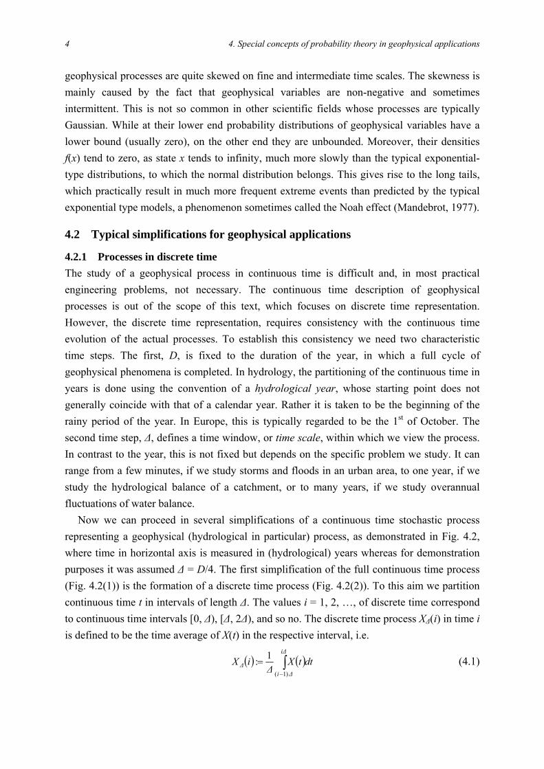
4.2.1 Processes in discrete time The study of a geophysical process in continuous time is difficult and, in most practical engineering problems, not necessary. The continuous time description of geophysical processes is out of the scope of this text, which focuses on discrete time representation. However, the discrete time representation, requires consistency with the continuous time evolution of the actual processes. To establish this consistency we need two characteristic time steps. The first, D, is fixed to the duration of the year, in which a full cycle of geophysical phenomena is completed. In hydrology, the partitioning of the continuous time in years is done using the convention of a hydrological year, whose starting point does not generally coincide with that of a calendar year. Rather it is taken to be the beginning of the rainy period of the year. In Europe, this is typically regarded to be the 1st of October. The second time step, ∆, defines a time window, or time scale, within which we view the process. In contrast to the year, this is not fixed but depends on the specific problem we study. It can range from a few minutes, if we study storms and floods in an urban area, to one year, if we study the hydrological balance of a catchment, or to many years, if we study overannual fluctuations of water balance. Now we can proceed in several simplifications of a continuous time stochastic process representing a geophysical (hydrological in particular) process, as demonstrated in Fig. 4.2, where time in horizontal axis is measured in (hydrological) years whereas for demonstration purposes it was assumed ∆ = D/4. The first simplification of the full continuous time process (Fig. 4.2(1)) is the formation of a discrete time process (Fig. 4.2(2)). To this aim we partition continuous time t in intervals of length ∆. The values i = 1, 2, …, of discrete time correspond to continuous time intervals [0, ∆), [∆, 2∆), and so no. The discrete time process X∆(i) in time i is defined to be the time average of X(t) in the respective interval, i.e.

( ) ( )∫−

=∆i

∆i∆ dttX

∆iX

)1(

1: ( 1) 4.

4.2 Typical simplifications for geophysical applications 5

For instance, if X(t) represents the instantaneous discharge of a river and ∆ is taken to be one day or one month, then X∆(i) represents the daily (more rigorously: the time averaged daily) or the monthly (more rigorously: the time averaged monthly) discharge, respectively. Sometimes, we wish to study the aggregated quantity, rather than the time average, in the corresponding time interval ∆, that is, the quantity

( 2) ( ) ( )∫−

=∆i

∆i∆ dttXiX

)1(

* : 4.

In this example, X*∆(i) represents the daily or the monthly runoff volume. Likewise, if X(t)

represents the instantaneous rainfall intensity in a specific point of a catchment and ∆ is taken as one day or one month, then X*

∆(i) represents the daily or the monthly rainfall depth, respectively. Even though time discretization is a step toward simplification of the study of a geophysical process, yet the mathematical description of X∆(i) or X*

∆(i) is complicated as it requires the analysis of periodicity and the autocorrelation of the process, for which the classical statistics, summarized in chapter 3, do not suffice. These issues are not covered in this text, except a few general discussions in the end of this chapter. The following simplifications, which are typical and useful in engineering problems, are more drastic and the resulting processes are easier to study using classical statistics. If we construct the process X∆(i) (or X*

∆(i)) assuming a time window equal to one year (∆ = D) then we obtain the annual process, XD(i) (or X*

D(i)); now i denotes discrete time in years (Fig. 4.2(3)). Thus,

( ) ( ) ( ) ( )∫∫−−

==iD

DiD

iD

DiD dttXiXdttX

DiX

)1(

*

)1(

:,1: ( 3) 4.

In this process the annual periodicity has been fully eliminated, because time intervals smaller than a year are not visible, and the process autocorrelation has been reduced significantly (but not eliminated), because of the large integration time step. This process, which represents the succession of an annual hydrological quantity (annual runoff, rainfall, evaporation, temperature) is very useful for problems of estimation of the water potential of an area. One way to move to a time interval smaller than a year, simultaneously eliminating the annual periodicity and significantly reducing autocorrelation is shown in Fig. 4.2(4). In each hydrological year i = 1, 2, …, we take an interval of length ∆ < D, specifically the interval

. Here j is a specified integer with possible values j = 1, 2, …,

D/∆ (in Fig. 4.2(4) it has been assumed j = 1). The process obtained is:

))1(,)1()1[( ∆jDi∆jDi +−−+−

( ) ( )( )

( )( ) ( )

( )

( )

∫∫+−

−+−

+−

−+−

==∆jDi

∆jDi∆

∆jDi

∆jDi∆ dttXiYdttX

∆iY

1

)1(1

*1

)1(1

:,1: ( 4) 4.


For instance if X(t) represents the instantaneous discharge of a river, ∆ is taken as one month, and j = 1, then Y∆(i) represents the average monthly discharge of the month of October of each hydrological year (assuming that it starts at the 1st of October) and Y*

∆(i) is the corresponding runoff volume.

4.2.2 Processes of extreme quantities In many problems, our interest is focused not of time averages, but on extreme quantities for a certain time interval, that is the maximum quantities (e.g. for flood studies) or the minimum quantities (e.g. for drought studies). For the study of these quantities we construct appropriate discrete time processes. Thus, Fig. 4.2(5) demonstrates the construction of the process of instantaneous annual maxima, Z0(i). In each year in a realization of the continuous time process X(t) we have taken only one value, the instantaneous maximum value that occurs during the entire year. We can extend this from the realization to the process and write

( ) ( ) tXiZiti <≤−

=10 max: ( 5) 4.

Likewise, we can define the process of instantaneous annual minima. Again in these processes the annual periodicity has been fully eliminated and the process autocorrelation has been reduced significantly. If, instead of instantaneous quantities, we are interested on an average during a time interval ∆, then we can construct and study the process of annual maxima on a specified time scale, i.e. (Fig. 4.2(6))

( ) ( ) ( ) ( )⎪⎭

⎪⎬⎫

⎪⎩

⎪⎨⎧

=⎪⎭

⎪⎬⎫

⎪⎩

⎪⎨⎧

= ∫∫+

−<≤−

+

−<≤−

∆s

s∆isi∆

∆s

s∆isi∆ dttXiZdttX∆

iZ1

*

1max:,1max: ( 6) 4.

This definition was based on the continuous time process X(t). Alternatively – but with smaller precision – it can be based on the already time discretized process X∆(i) (Fig. 4.2(7)):

( ) ( ) ( ) ( ) jXiZjXiZ ∆jjj∆∆jjj∆**

2121

max:,max:≤≤≤≤

=′=′ ( 7) 4.

where . Comparing Fig. 4.2(6) and Fig. 4.2(7), it is apparent that

Z

( ) ∆iDj∆Dij /:, 1/1: 21 =+−=

∆(i) και Z΄∆(i) are not identical in terms of the time position or their magnitude, but they do not differ much. Likewise, we construct the process of annual minima on a specified time scale. The typical values of the time interval ∆ in flood and drought studies vary from a few minutes (e.g. in design storm studies of urban drainage networks) to a few months (in water quality studies of rivers in drought conditions). A last series of maxima, known as series above threshold or partial duration series is demonstrated in Fig. 4.2(8), and can serve as a basis of the definition of the related processes. This is usually constructed from the discrete time process X∆(i), as in Fig. 4.2(7). The difference here is that instead of taking the maximum over each year, we form the series of all


values that exceed a threshold c, irrespectively of the location of these values in hydrological years, i.e.

( ) ( ) ( ) KK ,2,1,|:,2,1, =≥== jcjXjXiiW ∆∆∆ ( 8) 4.

0 1 2 3

0 1 2 3

0 1 2 30 1 2 3

0 1 2 3

0 1 2 3

0 1 2 3

0 1 2 3

X (t

)Y∆

(i)

Ζ0

(i)

XD

(i)

X∆

(i)

t

t t

t

t

t

t

t

Ζ∆

(i)

Ζ΄∆

(i)

W∆

(i)

(1)

(2)

(7)

(4) (8)

(3)

(6)

(5)

c

Fig. 4.2 Auxiliary sketch for the definition of the different types of stochastic processes; time t is in years.

Strictly speaking, the index i does not represent time, but it is just a the rank of the different variables W∆(i) in the time ordered series. The threshold c is usually chosen so that each year includes on the average one value greater than the threshold. Thus, in Fig. 4.2(8) the threshold, depicted as a horizontal dashed line, has been chosen so that it yields three values over three hydrological years. We observe that two values are located in the first year, none in the second year and one in the third year. With the above definition, it is possible that consecutive elements of the series correspond to adjacent time intervals, as in the two values


of the first year in our example. This may introduce significant stochastic dependence in the series. To avoid this, we can introduce a second threshold of a minimum time distance between consecutive elements of the series.

4.2.3 From stochastic processes to random variables As clarified above, this text does not cover the analysis of the complete geophysical processes either in continuous or discrete time. However, we have defined six other types of processes, in which the “time” index is discrete and may differ from actual time. Each of these processes includes one element per year, except of the process over threshold, which includes a variable number of elements per year, with an average of one per year. For our study, we shall make the following assumptions:

1. The processes are stationary: the distribution of each random variable remains the same from year to year.

2. The processes are ergodic: ensemble averages equal time averages. 3. The variables corresponding to different times are independent.

To clarify the meaning of these assumptions, we will discuss an example. Let X(t) represent the instantaneous discharge of a river at time t, and (according to the above notation) XD(τ) represent the mean annual discharge of (hydrological) year τ. Let us assume that 30 years of observations are available, so that we know the values xD(1), …, xD(30), which we regard as realizations of the random variables XD(1), …, XD(30). Obviously, for each of the variables XD(i) we can have (and we have) only one realization xD(i). In contrast to laboratory conditions, in nature we cannot repeat multiple experiments with different outcomes to acquire a sample for the same variable XD(i). Given the above observations, we can calculate time averages of certain quantities, for instance the standard sample average Dx

= [xD(1) + … + xD(30)]/30. Does this quantity give any information for the variable XD(31)? In general, the answer is negative. However, if assumptions 1 and 2 are valid, then Dx gives

important information for XD(31) and, thus, it helps make a statistical prediction. Specifically, under the stationarity assumption all XD(i) have the same statistical properties, and this provides grounds to treat them collectively; otherwise a quantity such as Dx would not have

any mathematical or physical meaning at all. Simultaneously, the stationarity assumption allows us to transfer any statistical property concerning the variables XD(1), …, XD(30) to the variable XD(31). The ergodicity assumption makes it possible to transform the time average

Dx to an estimate of the unknown true average of each of the variables XD(i), i.e. to estimate m = E[XD(i)] as Dx . So, both stationarity and ergodicity assumptions are fundamental and

powerful and allow us to make predictions of future events, e.g. E[XD(31)] = m. The third assumption, the independence, is not a fundamental one. It is just a simplification that makes possible the use of classical statistics. Otherwise, if the variables are dependent, the classical statistics need adaptations before they can be used (Koutsoyiannis, 2003).


It is important to stress that the stationarity assumption is not some property of the natural system under study, e.g. the river and its flow. It is an assumption about the mathematical model, i.e. the stochastic process, that we build for the natural system (Koutsoyiannis, 2006a). In this respect, it is related to the behaviour of the system but also to our knowledge of the system. For instance, let us assume that we have a reliable deterministic model of the evolution of the river discharge that predicts that at year 31 the average discharge will be xD(31) = 2m. If we build an additional stochastic model for our system, in an attempt to describe the uncertainty of this deterministic prediction, it will be reasonable to assume that E[XD(31)] = 2m, rather than E[XD(31)] = m. Thus, our process will be not stationary. Even without this hypothetical deterministic model, we can arrive to a similar situation if there is stochastic dependence among the consecutive variables. In case of dependence, the past observations affect our future predictions. In this situation, it is natural to use the conditional mean E[XD(31)|xD(1), …, xD(30)] instead of the unconditional mean E[XD(31)] = m as a prediction of the next year; the two quantities are different. Likewise, for year 32, given past information, the quantity E[XD(32)|xD(1), …, xD(30)] will be different both from E[XD(31)|xD(1), …, xD(30)] and m. In other words, dependence along with past observation make our model to behave as a nonstationary one in terms of conditional expectations, even though in an unconditional setting it is a stationary process (see also Koutsoyiannis et al., 2007). Under the assumptions of stationarity, ergodicity and independence, we can replace the notion of a stochastic process XD(t) with a unique realization xD(t), with the notion of a single underlying random variable XD with an ensemble of realizations xD(i), that are regarded as an observed sample of XD. In the latter case the time ordering of xD(i) does not matter at all.

4.2.4 A numerical investigation of the limits of the independence assumption We assume that, based on observational data of river discharge, we have concluded that the probability of the event of annual runoff volume smaller than 500 hm3* is very small, equal to 10−2. What is the probability that this event occurs for five consecutive years? Assuming stationarity, ergodicity and independence, this probability is simply =

10

52)10( −

−10. This is an extremely low probability: it means that we have to wait on the average 1010 or 10 billion years to see this event happen (by the way, the age of earth is much smaller than this duration). However, such events (successive occurrences of extreme events for multiyear periods) have been observed in several historical samples (see section 4.5.3). This indicates that the independence assumption is not a justified assumption and yields erroneous results. Thus we should avoid such an assumption if our target is to estimate probabilities for multiyear periods. Methodologies admitting dependence, i.e. based on the theory of stochastic

* We remind that the unit hm3 represents cubic hectometers (1 hm3 = (100 m)3 = 1 000 000 m3).


processes, are more appropriate for such problems and will result in probabilities much greater than 10−10; these however are out of the scope of this text. Now let us assume that for four successive years our extreme event has already occurred, i.e. that the runoff volume was smaller than 500 hm3 in all four years. What is the probability that this event will also occur in the fifth year? Many people, based on an unrefined intuition, may answer that the occurrence of the event already for four years will decrease the probability of another consecutive occurrence, and would be inclined to give an answer in between 10−2 and 10−10. This is totally incorrect. If we assume independence, then the correct answer is precisely 10−2; the past does not influence the future. If we assume positive dependence, which is a more correct assumption for natural processes, then the desired probability becomes higher than 10−2; it becomes more likely that a dry year will be followed by another dry year.

4.3 The concept of the return period

For a specific event A, which is a subset of some certain event Ω, we define the return period, T, as the mean time between consecutive occurrences of the event A. This is a standard term in engineering applications (in engineering hydrology in particular) but needs some clarification to avoid common misuses and frequent confusion. Under stationarity, if p is the probability of the event, then the return period T is related to p by

p∆

T 1= ( 9) 4.

4.

4.

where ∆ is the time interval on which the certain event Ω is defined or, for events defined on varying time frame, the mean interarrival time of the event Ω. For instance in panel (2) of Fig. 4.2, ∆ = D/4, whereas in panels (3)-(8) ∆ = D, as by construction all these cases involve one event Ω per year (either one exactly or one on the average). In particular, in panel (8), as discussed above, we have chosen the threshold c that defines our event Ω so that each year includes on the average one event. Had we chosen a smaller threshold, so that each year include two events on the average, the mean interarrival time of Ω would be ∆ = D/2. Apart from stationarity, no other conditions are needed for ( 9) to hold. To show this, we give the following general proof that is based on the simple identity P(CA) = P(C) – P(CB), valid for any events A and C, with B denoting the opposite event of A. We assume a stationary process in discrete time with time interval ∆. At time i, we denote as Ai the occurrence of the event A and as Bi the non occurrence. Because of stationarity P(A1) = P(A2) =… = P(A) = p (also P(B1) = P(B2) =… = P(B) = 1 – p). The time between consecutive occurrences of the event A is a random variable, say N, whose mean is the return period, T. Assuming that the event A has happened at time 0, if its next occurrence is at time n, we can be easily see that

PN = n = P(B1, B2, … Bn-1, An|A0) = P(A0, B1, B2, … Bn-1, An) / P(A0) ( 10)

4.3 The concept of the return period 11

or

PN = n = (1/p) P(A0, B1, B2, … Bn-1, An) ( 11) 4.

4.

4.

Obviously, T = E[N] ∆, where the expected value of N is (by definition)

E[N] = 1 P(N = 1) + 2 P(N = 2) + … (4.12)

Combining the last two equations we obtain

p E[N] = 1 P(A0, A1) + 2 P(A0, B1, A2) + 3 P(A0, B1, B2, A3) + … (4.13)

and using the above mentioned identity,

p E[N] = 1 [P(A0) – P(A0, B1)] + 2 [P(A0, B1) – P(A0, B1, B2)] + + 3 [P(A0, B1, B2) – P(A0, B1, B2, B3)] + … (4.14)

or

p E[N] = P(A0) + P(A0, B1) + P(A0, B1, B2) + … (4.15)

Using once more the same identity, we find

p E[N] = [1 – P(B0)] + [P(B1) – P(B0, B1)] + [P(B1, B2) – P(B0, B1, B2)] + … (4.16)

and observing that, because of stationarity, P(B0) = P(B1), P(B0, B1) = P(B1, B2), etc., we conclude that

p E[N] = 1 ( 17)

which proves (4.9). From this general proof we conclude that (4.9) holds true either if the process is time independent or dependent, whatever the dependence is. (In most hydrological and engineering texts, e.g. Kottegoda, 1980, p. 213; Kottegoda and Rosso, 1998, p. 190; Koutsoyiannis, 1998, p. 96, independence has been put as a necessary condition for ( 9) to be valid). All this analysis is valid for processes in discrete time; as the time interval ∆, on which the event A is defined, tends to zero, the return period will tend to zero too, provided that the probability of A is finite. Extreme events that are of interest in geophysics (and hydrology) are usually of two types, highs (floods) or lows (droughts). In the former case the event we are interested is the exceedence of a certain value x, i.e. X > x, which is characterized by the probability of exceedence, ( )xFxXPxFp XX −=>== 1)(* . In the latter case the event we are interested is

the non exceedence of a certain value x, i.e. X ≤ x, which is characterized by the probability of non exceedence, . As the processes that we deal with here are

defined on the annual scale (∆ = D), for an exceedence event (high flow) we have

)( xXPxFp X ≤==

( )xFxFxXPDT

XX −==

>=

11

)(1

1

* ( 18) 4.

whereas for a non exceedence event (drought) we have


)(

1

1xFxXPD

TX

=≤

= ( 19) 4.

Sometimes we write the above relationships omitting D = 1 year, as it is very common to express the return period in years (essentially identifying T with E[N]). However, the correct (dimensionally consistent) forms are those written in equations (4.18)-(4.19). Sometimes (4.18) has been used as a definition of the return period, saying that the return period is the reciprocal of the exceedence probability. This again is not dimensionally consistent (given that return period should have dimensions of time) nor general enough (it does not cover the case of low flows). The term return period should not trap us to imply that there is any periodic behaviour in consecutive occurrences of events such as in exceedence or nonexceedences of threshold values in nature. In a stochastic process the time between consecutive occurrences of the event is a random variable, N, whose mean is the return period, T. For example, if the value 500 m3/s of the annual maximum discharge in a river has a return period of 50 years, this does not mean that this value would be exceeded periodically once every 50 years. Rather it means that the average time between consecutive exceedences will be 50 years. An alternative term that has been used to avoid “period” is recurrence interval. However, sometimes (e.g. in Chow et al., 1988) this term has been given the meaning of the random variable N and not its mean T. Typical values used in engineering design of flood protection works are given in Table 4.1.

Table 4.1 Return periods most commonly used in hydrological design for high flows and corresponding exceedence and nonexceedence probabilities.

Return period T (years)

Exceedence probability F* (%)

Nonexceedence probability F (%)

2 50 50 5 20 80

10 10 90 20 5 95 50 2 98

100 1 99 500 0.2 99.8

1000 0.1 99.9 5 000 0.02 99.98

10 000 0.001 99.99 Note: To adapt the table for low flow events we must interchange

the columns exceedence probability and nonexceedence

probability.

4.4 The concept of risk 13

4.4 The concept of risk

Depending on the context, risk can be defined to be either a probability of failure or the product of probability of failure times the losses per failure. Here we use the former definition. A failure is an event that usually occurs when the load L, exceeds the capacity C of a construction. In the design phase, the design capacity is larger than the design load, so as to assure a certain safety margin

LC −=:SM > 0 (4.20)

or a certain safety factor

LC

=:SF > 1 (4.21)

In engineering hydrology, L could be, for instance, the design flood discharge of a dam spillway whereas C is the discharge capacity of the spillway, that is the discharge that can be routed through the spillway without overtopping of the dam. In most empirical engineering methodologies both L and C are treated in a deterministic manner regarding them as fixed quantities. However, engineers are aware of the intrinsic natural uncertainty and therefore are not satisfied with a safety factor as low as, say, 1.01, even though in a deterministic approach this would suffice to avoid a failure. Rather, they may adopt a safety factor as high as 2, 3 or more, depending on empirical criteria about the specific type of structure. However, the empirical deterministic approach is more or less arbitrary, subjective and inconsistent. The probability theory can quantify the uncertainty and the risk and provide more design criteria. According to a probabilistic approach SM and SF are regarded as random variables and the risk is defined to be:

R := PSF < 1 = PSM < 0 (4.22)

and its complement, 1 – R is known as reliability. In the most typical problems of engineering hydrology, the design capacity (e.g. discharge capacity or storage capacity) could be specified with certainty (C = c), and is not regarded as a random variable. However, the load L should be taken as a random variable because of the intrinsic uncertainty of natural processes. In this case, the risk is

1 cLPcLPR ≤−=>= ( 23) 4.

The probability PL ≤ c (the reliability) depends on the variability of the natural process (e.g. the river discharge, the fixed quantity c, and the life time of the project n D (n years). With the notation of section 4.2.2, assuming an appropriate time window ∆ for the phenomenon studied, the event L ≤ c (which refers to the n year period) is equivalent to the event Z∆(1) ≤ c, …, Z∆(n) ≤ c. Assuming independence of Z∆(i) trough years, it is concluded that


( ) n

Ζn

∆ cFcZPR∆

][1][1 −=≤−= ( 24) 4.

4.

where is the distribution function of the annual flood. Expressing it in terms of the

return period T from ( 18), we obtain the following relationship that relates the three basic quantities of engineering design, the risk R, the return period T and the life time n years:

( )∆Ζ

F

n

TDR ⎟⎠⎞

⎜⎝⎛ −−= 11 ( 25) 4.

4.

4.

Graphical depiction of (4.25) is given in Fig. 4.3 for characteristic return periods. Given that , the following approximation of ( 25), with

error < 1% for T ≥ 50, is obtained:

( ) ( ) ( ) nxxxnxnx n −≈−−−=−=− L2/1ln1ln 2

( 26) TnDeR /1 −−≈

T= 2

5

10

20

50

100

200

500

000 1

000 2

000 5

000 100.0001

0.001

0.01

0.1

1

1 10 100 1000

R

n Fig. 4.3 Graphical depiction of the interrelationship of the characteristic quantities of engineering design (equation 4.25).

Solving (4.25) for T we obtain the following relationship that gives the required return period for given design risk and design life time:

( ) nR

DT /111 −−= ( 27) 4.

All equations (4.24)-(4.27) are based on the assumption of independence and are not valid in case of dependence. To get an idea of the effect of dependence, let us examine the limiting

4.5 An introduction to dependence, persistence and antipersistence 15

case of complete dependence, in which the occurrence of a single event Z∆(1) ≤ c entails that all Z∆(i) ≤ c. It is easy to see that in this case we should substitute 1 for n in all equations. Thus, (4.27) becomes T = D/R so that it will yield a return period smaller than that estimated by (4.27) if the risk is specified. In other words, if we use (4.27) we are on the safe side in the case that there is dependence in the process.

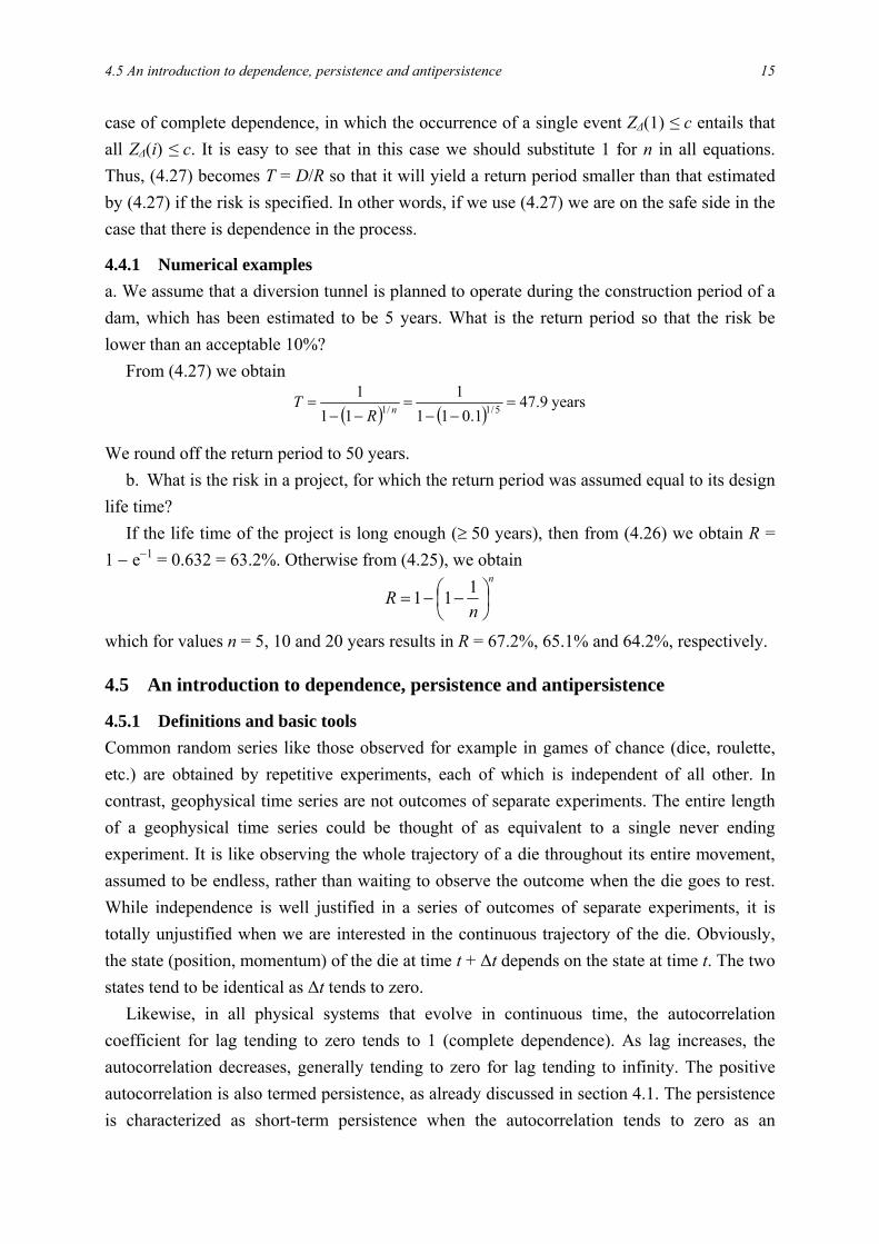
4.4.1 Numerical examples a. We assume that a diversion tunnel is planned to operate during the construction period of a dam, which has been estimated to be 5 years. What is the return period so that the risk be lower than an acceptable 10%? From (4.27) we obtain

( ) ( )years 9.47

1.0111

111

5/1/1 =−−

=−−

= nRT

We round off the return period to 50 years. b. What is the risk in a project, for which the return period was assumed equal to its design life time? If the life time of the project is long enough (≥ 50 years), then from (4.26) we obtain R = 1 − e−1 = 0.632 = 63.2%. Otherwise from (4.25), we obtain

n

nR ⎟

⎠⎞

⎜⎝⎛ −−=

111

which for values n = 5, 10 and 20 years results in R = 67.2%, 65.1% and 64.2%, respectively.

4.5 An introduction to dependence, persistence and antipersistence

4.5.1 Definitions and basic tools Common random series like those observed for example in games of chance (dice, roulette, etc.) are obtained by repetitive experiments, each of which is independent of all other. In contrast, geophysical time series are not outcomes of separate experiments. The entire length of a geophysical time series could be thought of as equivalent to a single never ending experiment. It is like observing the whole trajectory of a die throughout its entire movement, assumed to be endless, rather than waiting to observe the outcome when the die goes to rest. While independence is well justified in a series of outcomes of separate experiments, it is totally unjustified when we are interested in the continuous trajectory of the die. Obviously, the state (position, momentum) of the die at time t + ∆t depends on the state at time t. The two states tend to be identical as ∆t tends to zero. Likewise, in all physical systems that evolve in continuous time, the autocorrelation coefficient for lag tending to zero tends to 1 (complete dependence). As lag increases, the autocorrelation decreases, generally tending to zero for lag tending to infinity. The positive autocorrelation is also termed persistence, as already discussed in section 4.1. The persistence is characterized as short-term persistence when the autocorrelation tends to zero as an


exponential function of lag time and as log-term persistence when the autocorrelation tends to zero as a power-law function of lag time. The latter case corresponds to stronger or longer tail of the autocorrelation function. Sometimes, for intermediate lags negative autocorrelations may appear. The general behaviour corresponding to this case is known as antipersistence. An easier means to explain antipersistence and persistence, short- or long-term, is provided by studying the variation of the standard deviation with time scale. To avoid the effect of seasonality, here we consider time scales ∆ that are integer multiples of the annual time scale, i.e., ∆ = k D, k = 1, 2, … (4.28)

By virtue of (4.1), which holds for any ∆ (also for ∆ > D), we easily obtain that the process at scale ∆ is related to that at scale D by

XkD(i) = [XD(ik – k + 1) + … + XD(ik)]/k ( 29)

( 29)

4.

4.

This is nothing other than the time average of a number k of consecutive random variables. We can define similar time average processes for over-annual scales also for the other cases (Y and Z) that we discussed in section 4.2. For k sufficiently large (typically 30, even though sometimes k = 10 has been also used), such processes represent what we call climate; ∆ = 30 years is the typical climatic time scale. However, here we will regard ∆ as varying and we will study the variation of the standard deviation of X∆(i) with ∆ = kD. Let σ∆ ≡ σkD denote the standard deviation at scale ∆ = kD, i.e. σkD := StD[XkD(i)]. According to XkD(i) is the average of k random variables. If these variables are independent, then we know from chapter 3 that

kσ

σ DkD = or

∆Dσσ D∆ = ( 30) 4.

where σD is the standard deviation at scale 1. This provides a means to test whether or not the process at hand is independent in time. If it is independent, then the double logarithmic plot of σ∆ vs. ∆ will be a straight line with slope –0.5. Milder negative slopes (>–0.5) indicate persistence and steeper slopes (<–0.5) indicate antipersistence. Short-term persistence is manifested in the plot as a curve with mild slope for small k, which asymptotically tends to -0.5 for large k. In long-term persistence the slope remains milder than –0.5 even for large k. A more generalized law that asymptotically (for large k) holds in cases of long-term persistence and antipersistence is given by

HD

kD kσσ −∝ 1 or

H

D∆ ∆Dσσ

−

⎟⎠⎞

⎜⎝⎛∝

1

( 31) 4.

The coefficient H is termed the Hurst coefficient, after Hurst (1951) who discovered the


long-term persistence in geophysical time series*. Clearly, H = 1 + d, where d is the slope of the plot of σ∆ vs. ∆. Generally, for stationary processes, 0 < H < 1 (Mandelbrot and van Ness, 1968). For independent processes, H = 0.5; for persistent processes, 0.5 < H < 1 and for antipersistent processes, 0 < H < 0.5. For persistent processes it is possible that the law holds as an equality for any k. Mathematically, this is also possible for antipersistent processes (H < 0.5) but physically it is not realistic. To see the reason why this happens, we assume that the law holds as an equality for any k; in this case it defines a stochastic process termed a simple scaling stochastic (SSS) process. It can be shown (e.g. Koutsoyiannis, 2002) that the autocorrelation X

( 31)

( 31)

4.

4.

4.

kD(i) of the process for scale kD and lag j, i.e.

the quantity ρkD(j) := Cov[XkD(i), XkD(i + j)] / Var[X(k)i ]), is given by

ρkD(j) = ρ(j) = (1/2) (|j + 1|2H + |j – 1|2H) – |j|2H ( 32)

This shows that the autocorrelation is independent of scale. Inspection shows that if H > 0.5 the autocorrelation for any lag is positive (persistence), whereas if H < 0.5 the autocorrelation for any lag is negative (antipersistence). In the latter case it takes the most negative values at lag j = 1, which is ρkD(1) = ρ(1) = 22H –1 – 1. However, physical realism demands that for small scales and lags, the autocorrelation should be positive. Given a time series of sufficient length n at time scale D, we can test in a simple way whether the law (4.30) is fulfilled or not, and if not, we can see whether the time series implies persistence or antipersistence. To this aim, we can estimate from the time series the standard deviation σkD for several values of k. Assuming k = 1, we estimate σD from the n data values available. For k = 2 (and assuming for simplicity that the series length n is even) we can construct a size (n/2) sample X2D(1) = [XD(1) + XD(2)]/2, X2D(2) = [XD(3) + XD(4)]/2, …, X2D(n/2) = [XD(n – 1) + XD(n)]/2. From these we can estimate σ2D. Proceeding this way (e.g. X3D(1) = [XD(1) + XD(2) + XD(3)]/3, etc.) we can estimate σkD for k up to, say, n/10 (in order to have 10 sample values for the estimation of standard deviation). Constructing a logarithmic plot of the estimate of standard deviation σkD versus k we can test graphically the validity of the statistical law (4.30) and estimate the coefficient H of law (4.31).

4.5.2 Synthetic examples Now we will demonstrate the above concepts with the help of a few examples. We will start with the synthetic example that was already studied in chapter 1. Although this example is referred to a fully deterministic system, it is useful in understanding the behaviours discussed; besides, the statistical analyses outlined above can be applied also in time series that result from deterministic systems. It is reminded that the working example of chapter 1 examines a hypothetical plain with water stored in the soil, which sustains some vegetation. Each year a

* Hurst used a different formulation of this behaviour, based on the so-called rescaled range. The formulation in terms of standard deviation at the time scale kD, as in equation (4.31), is much simpler yet equivalent to Hurst’s (see theoretical discussion by Beran, 1994, p. 83, and practical demonstration by Koutsoyiannis, 2002, 2003).


constant amount of water enters the soil and the potential evapotranspiration is also constant, but the actual evapotranspiration varies following the variation of the vegetation cover f. The vegetation cover and the soil water storage s are the two state variables of the system that vary in time i; the system dynamics are expressed by very simple equations.

-2000

-1500

-1000

-500

0

500

1000

1500

2000

0 100 200 300 400 500 600 700 800 900 1000i

s i Series of storageMoving average of 30 values

Fig. 4.4 Graphical depiction of the evolution of the system storage si (in mm) of the working example in chapter 1 for time up to 1000.

-2000

-1500

-1000

-500

0

500

1000

1500

2000

0 100 200 300 400 500 600 700 800 900 1000i

s i Random seriesMoving average of 30 values

Fig. 4.5 Graphical depiction of a series of random numbers in the interval (-800, 800) having mean and standard deviation equal to those of the series in Fig. 4.4.

In chapter 1, Fig. 1.3, we have seen a graphical depiction of the system evolution for certain initial conditions that we called the “true” conditions. Now in Fig. 4.4 we depict the continuation of this evolution of the storage s(i) (or si) for time up to 1000. In addition, we have given in Fig. 4.4 a plot of the 30-year moving average* of si, which shows that this

* The moving average is the average of k random variables consecutive in time, as in (4.29). However, for better illustration, here we used a slightly different definition, i.e., X30D(i) = [XD(i – 15) + … + XD(i + 14)]/30.


moving average is almost a horizontal straight line at s = 0. The experienced eye may recognize from this, without the need of further tools, a strongly antipersistent behaviour. For comparison we have derived a random series* with mean and standard deviation equal to those of the original series, and we plotted it in Fig. 4.5. Comparing the plots of moving averages in Fig. 4.4 and Fig. 4.5 we see a clear difference. In the former case (antipersistence) the plot is virtually a horizontal straight line, whereas in the latter case (pure randomness) it is a curly line, which however does not depart very much from the line s = 0. Sometimes antipersistence has been confused with periodicity or cyclic behaviour. However, periodicity would imply that the time between consecutive peaks in the time series would be constant, equal to the period of the phenomenon. To distinguish the two behaviours, we have calculated a series of times between peaks, τ, from the time series of our example, which for better accuracy we extended up to 10 000 items by the same algorithm. From this series we constructed an histogram of times between peaks, which is shown in Fig. 4.6. We see that the time between peaks varies from 4 to 22 years, with a mode of 6 years. Clearly, this behaviour is totally different from a periodic phenomenon, and is better described by the term antipersistence.

0

0.02

0.04

0.06

0.08

0.1

0.12

0.14

0.16

1 2 3 4 5 6 7 8 9 10 11 12 13 14 15 16 17 18 19 20 21 22 23

τ

ν

Fig. 4.6 Relative frequency ν of the time τ between consecutive peaks, estimated from a series of 10 000 items of a series of si of the example system.

* This series has been produced as follows: First, we derive a series of integer random numbers qi by the recursive relationship qi = κ qi – 1 mod λ, where κ = 75, λ = 231 – 1, q0 = 78910785 and mod is the modulo operator that finds the remainder of an integer division. Then, we derive a series of real numbers in the interval [0, 1) as ri = qi / λ. We obtain the final series si by si = c(2qi – 1), where c = 600.


The same example system helps us to acquire an idea of persistence. To this aim we have constructed and plotted in 1000 terms of the time series of the peaks pFig. 4.7 j of the time series si. Now we see in Fig. 4.7 that the moving average of 30 values exhibits large and long excursions from the overall mean, which is about 800 (not plotted). These excursions are the obvious manifestation of persistence.

0

500

1000

1500

2000

0 100 200 300 400 500 600 700 800 900 1000

j

p j

Series of peaksMoving average of 30 values

Fig. 4.7 Graphical depiction of a series of peaks pj (in mm) of the soil storage si; here j does not denote time but the rank of each peak in time order.

However, a better depiction and quantification of the persistence and antipersistence is provided by the plot of standard deviation σ∆ vs. time scale ∆, as described in section 4.5.1.

gives such plots for the series of storage shown in Fig. 4.4 (but for 10 000 items) and for the random series of Fig. 4.5 (also for 10 000 items). Clearly, the plot of the random series shows a straight line arrangement with slope –0.5, which corresponds to a Hurst coefficient H = 1 – 0.5 = 0.5 (as expected). The plot of the storage time series is more interesting. For low scales (∆ ≤ 4) the slope in the arrangement of the points is very low, indicating a positive dependence at small lags. However, for large scales (∆ ≥ 20), a straight line arrangement of points appears, which has large slope, equal to –0.98. This corresponds to a Hurst coefficient H = 1 – 0.98 = 0.02, which indicates very strong antipersistence.

Fig. 4.8

Fig. 4.8

Likewise, gives a similar plot for the series of peaks shown in Fig. 4.7, also in comparison with that of the random series. The plot of the series of peaks shows a straight line arrangement of points for low and high ∆, which has very low slope, equal to –0.02. This corresponds to a Hurst coefficient H = 1 – 0.02 = 0.98, which indicates very strong persistence.

Fig. 4.9

We can observe in that for scale ∆ = 1 the standard deviation of the series of storage is significantly greater than that of the random series, despite the fact that the latter was constructed so as to have the same mean and standard deviation with the former. This is because, after the expansion of the two series from 1000 to 10 000 items, σD of the storage series increased significantly whereas σD of the random series remained in the same level. The


large persistence in the peaks results in high fluctuations of standard deviation and this was the reason for the increased σD of the storage time series.

Slope - 0.98

Slope -0.5

1

10

100

1000

1 10 100 1000∆

σ ∆

Series of storageRandom series

Fig. 4.8 Standard deviation σ∆ (in mm) vs. time scale ∆ plot of the series of storage shown in Fig. 4.4 (but for 10 000 items) in comparison with that of the random series of Fig. 4.5 (also for 10 000 items).

Slope -0.02

Slope -0.5

10

100

1000

1 10 100 1000∆

σ ∆

Series of peaksRandom series

Fig. 4.9 Standard deviation σ∆ (in mm) vs. scale ∆ plot of the series of peaks shown in Fig. 4.7 in comparison with that of the random series of Fig. 4.5 (also shown in Fig. 4.8).


4.5.3 Real world examples It is not easy to find real world examples with antipersistent behaviour. However, there are a few phenomena with such behaviour which are commonly called “oscillations”. The most widely known is the El Niño Southern Oscillation (ENSO), a fluctuation of air pressure and water temperature between the southeastern and southwestern Pacific. Typically it is quantified by the so-called Southern Oscillation Index (SOI), which expresses the difference in the air pressure between Tahiti (an island in French Polynesia) and Darwin (North Australia); this difference is typically standardized in monthly scale by monthly mean and standard deviation. Here, instead of SOI, we have used the raw time series of the air pressure in Tahiti*, to avoid the artificial effects of taking differences and standardizing, and we have averaged the monthly time series on annual basis to discard the effect of the annual cycle. The annual series has been plotted in , where the antipersistent behaviour becomes apparent from the 30-year moving average, which is virtually an horizontal straight line. The same behaviour is also apparent in Fig. 4.11, which shows the plot of standard deviation σ

Fig. 4.10

∆ vs. time scale ∆. For large scales (∆ ≥ 2 years), a straight line arrangement of points appears, which has high slope, equal to –0.8. This corresponds to a Hurst coefficient H = 1 – 0.8 = 0.2, which indicates strong antipersistence. The figure also shows a series of points that were derived from the monthly time series. For large scales, the monthly plot is virtually the same with the annual plot. For low time scales, the monthly plot clearly shows a low slope, which manifests the combined effect of the annual cycle and positive autocorrelation for small lags at the monthly scale (even for the annual scale, the lag one autocorrelation is positive, 0.18). Generally, the figure resembles Fig. 4.8.

1010

1011

1012

1013

1014

1015

1870 1890 1910 1930 1950 1970 1990 2010

Year

x

Annual series30-year moving average

Fig. 4.10 Graphical depiction of the mean annual air pressure in Tahiti (in hPa), which is one of the two variables used to define the Southern Oscillation Index (SOI).

* The series is available online at ftp://ftp.bom.gov.au/anon/home/ncc/www/sco/soi/tahitimslp.html on a monthly scale.


Slope -0.80

Slope -0.5

0.1

1

10

0.01 0.1 1 10 100∆

σ∆

Aggregated fromannual series

Aggregated frommonthly series

Model forindependent series

Fig. 4.11 Plot of standard deviation σ∆ (in hPa) vs. scale ∆ (in years) for the series of air pressure in Tahiti shown in Fig. 4.10.

While antipersistence is very rarely seen in nature, persistence is a very common behaviour, which however requires long time series to be observed. Long-term persistence has been found to be omnipresent in several long time series such as meteorological and climatological (temperature at a point, regional or global basis, wind power, proxy series such as tree ring widths or isotope concentrations) and hydrological (particularly river flows), but it has been also reported in diverse scientific fields such as biology, physiology, psychology, economics, politics and Internet computing (Koutsoyiannis and Montanari, 2007). Thus, it seems that in real world processes this behaviour is the rule rather than the exception. The omnipresence can be explained based either on dynamical systems with changing parameters (Koutsoyiannis, 2006b) or on the principle of maximum entropy applied to stochastic processes at all time scales simultaneously (Koutsoyiannis, 2005). The example we study here is the most common one and refers to the longest available instrumental data series. This is the annual minimum water level of the Nile river for the years 622 to 1284 AD (663 observations), measured at the Roda Nilometer near Cairo (Beran, 1994)*. The time series is plotted in Fig. 4.12, where the long excursions of the 30-year moving average from the overall mean are apparent. As discussed above, the large fluctuations at large scales distinguishes the time series from random noise and is the signature of long-term persistence.

* The data are available from http://lib.stat.cmu.edu/S/beran.


800

900

1000

1100

1200

1300

1400

1500

600 700 800 900 1000 1100 1200 1300

Year AD

x

Annual series 30-year moving average

Fig. 4.12 Graphical depiction of the time series of the minimum annual water level at the Roda Nilometer (in cm) for the years 622 to 1284 AD (663 years).

The persistence is also apparent in Fig. 4.13, which shows the plot of standard deviation σ∆ vs. time scale ∆. Here, the straight line arrangement of points appears on all scales, which makes the law (4.31) valid virtually on all scales. The slope equals –0.14 and it corresponds to a Hurst coefficient H = 1 – 0.14 = 0.86, which indicates strong persistence.

Slope -0.14

Slope -0.5

10

100

1 10∆

σ∆

100

NilometerModel for independent series

Fig. 4.13 Plot of standard deviation σ∆ (in cm) vs. scale ∆ (in years) for the Nilometer minimum annual water lever time series shown in Fig. 4.12.


References Beran, J., Statistics for Long-Memory Processes, Monographs on Statistics and Applied

Probability, vol. 61. Chapman & Hall, New York1994.. Chow, V. T., D. R. Maidment, and L. W. Mays, Applied Hydrology, McGraw-Hill, 1988. Haan, C. T., Statistical Methods in Hydrology, The Iowa State University Press, USA, 1977. Hurst, H.E., Long term storage capacities of reservoirs. Transactions ASCE, 116, 776–808,

1951. Kottegoda, N. T., Stochastic Water Resources Technology, Macmillan Press, London, 1980. Kottegoda, N. T., and R. Rosso, Statistics, Probability and Reliability for Civil and

Environmental Engineers, McGraw-Hill, New York, 1998. Koutsoyiannis, D., Statistical Hydrology, Edition 4, 312 pages, National Technical University

of Athens, Athens, 1997 (in Greek). Koutsoyiannis, D., The Hurst phenomenon and fractional Gaussian noise made easy,

Hydrological Sciences Journal, 47(4), 573-595, 2002. Koutsoyiannis, D., Climate change, the Hurst phenomenon, and hydrological statistics,

Hydrological Sciences Journal, 48(1), 3-24, 2003. Koutsoyiannis, D., Uncertainty, entropy, scaling and hydrological stochastics, 2, Time

dependence of hydrological processes and time scaling, Hydrological Sciences Journal, 50(3), 405-426, 2005.

Koutsoyiannis, D., Nonstationarity versus scaling in hydrology, Journal of Hydrology, 324, 239-254, 2006a.

Koutsoyiannis, D., A toy model of climatic variability with scaling behaviour, Journal of Hydrology, 322, 25-48, 2006b.

Koutsoyiannis, D., A. Efstratiadis, and K. Georgakakos, Uncertainty assessment of future hydroclimatic predictions: A comparison of probabilistic and scenario-based approaches, Journal of Hydrometeorology, 8(3), 261-281, 2007.

Koutsoyiannis, D., and A. Montanari, Statistical analysis of hydroclimatic time series: Uncertainty and insights, Water Resources Research, 43(5), W05429.1-9, 2007.

Mandelbrot, B. B., The Fractal Geometry of Nature, 248 pages, Freeman, New York, USA, 1977.

Mandelbrot, B.B., and J.W. van Ness, Fractional Brownian Motion, fractional noises and applications, SIAM Review, 10, 422 – 437, 1968.

Documents

Special concepts of probability theory in geophysical ... · Special concepts of probability theory in geophysical applications ... + Ξ(t), where d(t) is a deterministic periodical