A Survey of Probability Concepts

Ka-fu WONG

5 July 2007

Abstract

All of us should have learned some basic concepts of probability in high school. This chapter serves as areview of those concepts that we have long forgotten. Students should not underestimate the importanceof such review. These probability concepts are central to the understanding of other concepts in thiscourse. Students should practice a lot until they can solve the problems in reasonable speed. Usually, ifwe really understand the concepts well, we can solve the problem in reasonable speed.

Suppose we close our eyes and randomly select a student from this class. What is the gender of this

student, i.e., female or male? Yes, this person has to be either male or female. Okay. I will say “male”. Is

there a reason I choose “male” instead of “female”? Yes, because there are more male in this class. How

likely will my guess be wrong? If 60% of the class are male, my guess will be wrong 40% of the times –

if this experiment is repeated many times, say, 1,000 times, I will be wrong in approximately 400 of the

experiments.

Let me rephrase the question: How likely is the selected person a male? If 60% of the class are male,

the selected person will be a male 60% of the times – if this experiment is repeated many times, say, 1,000

times, approximately 600 of the experiments will turn out to be male.

Simulation 1 (Guessing gender): We will like to simulate the process of drawing one student

from a class of 100 students, 60 of them are male and 40 of them are female. Since there are

more male than female in the class, our best prediction is always male. And, check how often we

make the correct prediction and mistake.

Doing this kind of simulation in a class is too time-consuming. It is much easier and faster to

mimic the in-class simulation using a computing software, such as Excel.

1. Create an artificial list of 100 students labelled 1 to 100 (say, in the first column of excel).

Create a variable gender and code 1 (male) for the students labelled 1 to 60, and 0 (female)

otherwise (say, in the second column). Assign the probability of each student being picked

as 1/100 (say, in the third column)

1

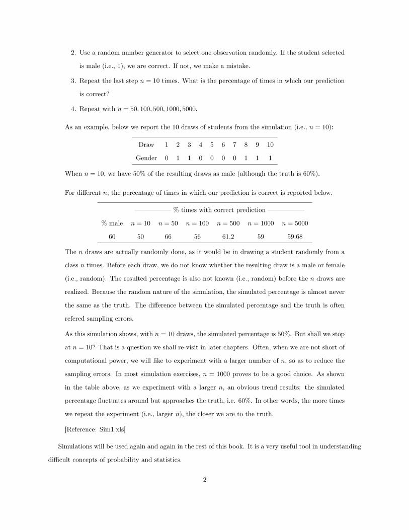
2. Use a random number generator to select one observation randomly. If the student selected

is male (i.e., 1), we are correct. If not, we make a mistake.

3. Repeat the last step n = 10 times. What is the percentage of times in which our prediction

is correct?

4. Repeat with n = 50, 100, 500, 1000, 5000.

As an example, below we report the 10 draws of students from the simulation (i.e., n = 10):

Draw 1 2 3 4 5 6 7 8 9 10

Gender 0 1 1 0 0 0 0 1 1 1

When n = 10, we have 50% of the resulting draws as male (although the truth is 60%).

For different n, the percentage of times in which our prediction is correct is reported below.

—————– % times with correct prediction —————–

% male n = 10 n = 50 n = 100 n = 500 n = 1000 n = 5000

60 50 66 56 61.2 59 59.68

The n draws are actually randomly done, as it would be in drawing a student randomly from a

class n times. Before each draw, we do not know whether the resulting draw is a male or female

(i.e., random). The resulted percentage is also not known (i.e., random) before the n draws are

realized. Because the random nature of the simulation, the simulated percentage is almost never

the same as the truth. The difference between the simulated percentage and the truth is often

refered sampling errors.

As this simulation shows, with n = 10 draws, the simulated percentage is 50%. But shall we stop

at n = 10? That is a question we shall re-visit in later chapters. Often, when we are not short of

computational power, we will like to experiment with a larger number of n, so as to reduce the

sampling errors. In most simulation exercises, n = 1000 proves to be a good choice. As shown

in the table above, as we experiment with a larger n, an obvious trend results: the simulated

percentage fluctuates around but approaches the truth, i.e. 60%. In other words, the more times

we repeat the experiment (i.e., larger n), the closer we are to the truth.

[Reference: Sim1.xls]

Simulations will be used again and again in the rest of this book. It is a very useful tool in understanding

difficult concepts of probability and statistics.

2

1 We all know some probabililty

We all understand probability to some extent. Let’s try to work on some simple questions in the next section.

Answers will be provide in following section. Please do not look at the answers before you have tried your

best. Most of us should be able to solve if we are willing to spend time on them. We shall refer back to

these examples when we encounter difficulty in understanding some other concepts or examples.

1.1 Three challenages

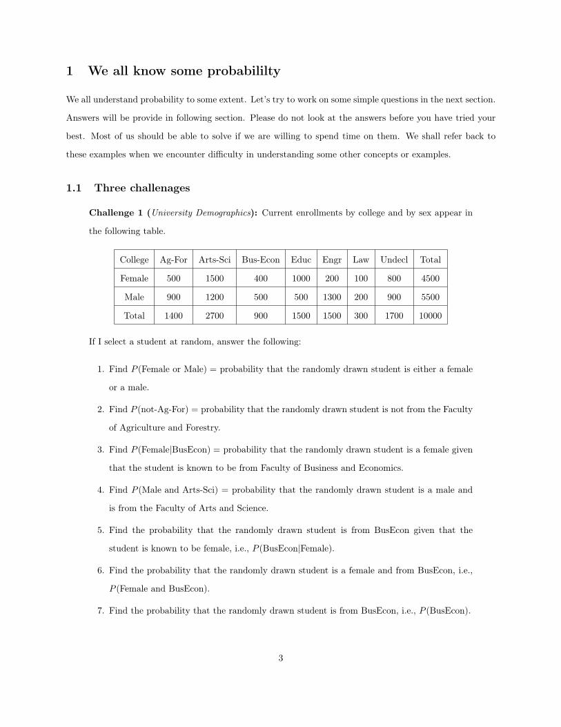
Challenge 1 (University Demographics): Current enrollments by college and by sex appear in

the following table.

College Ag-For Arts-Sci Bus-Econ Educ Engr Law Undecl Total

Female 500 1500 400 1000 200 100 800 4500

Male 900 1200 500 500 1300 200 900 5500

Total 1400 2700 900 1500 1500 300 1700 10000

If I select a student at random, answer the following:

1. Find P (Female or Male) = probability that the randomly drawn student is either a female

or a male.

2. Find P (not-Ag-For) = probability that the randomly drawn student is not from the Faculty

of Agriculture and Forestry.

3. Find P (Female|BusEcon) = probability that the randomly drawn student is a female given

that the student is known to be from Faculty of Business and Economics.

4. Find P (Male and Arts-Sci) = probability that the randomly drawn student is a male and

is from the Faculty of Arts and Science.

5. Find the probability that the randomly drawn student is from BusEcon given that the

student is known to be female, i.e., P (BusEcon|Female).

6. Find the probability that the randomly drawn student is a female and from BusEcon, i.e.,

P (Female and BusEcon).

7. Find the probability that the randomly drawn student is from BusEcon, i.e., P (BusEcon).

3

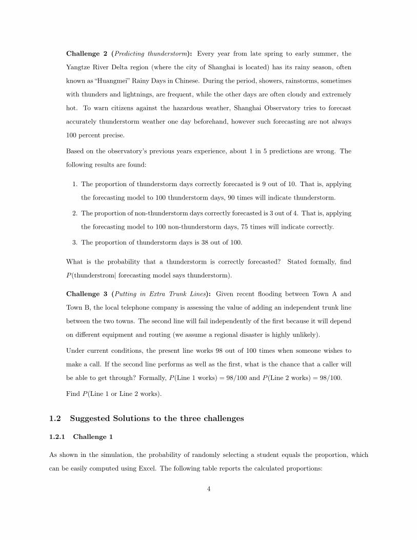
Challenge 2 (Predicting thunderstorm): Every year from late spring to early summer, the

Yangtze River Delta region (where the city of Shanghai is located) has its rainy season, often

known as “Huangmei” Rainy Days in Chinese. During the period, showers, rainstorms, sometimes

with thunders and lightnings, are frequent, while the other days are often cloudy and extremely

hot. To warn citizens against the hazardous weather, Shanghai Observatory tries to forecast

accurately thunderstorm weather one day beforehand, however such forecasting are not always

100 percent precise.

Based on the observatory’s previous years experience, about 1 in 5 predictions are wrong. The

following results are found:

1. The proportion of thunderstorm days correctly forecasted is 9 out of 10. That is, applying

the forecasting model to 100 thunderstorm days, 90 times will indicate thunderstorm.

2. The proportion of non-thunderstorm days correctly forecasted is 3 out of 4. That is, applying

the forecasting model to 100 non-thunderstorm days, 75 times will indicate correctly.

3. The proportion of thunderstorm days is 38 out of 100.

What is the probability that a thunderstorm is correctly forecasted? Stated formally, find

P (thunderstrom| forecasting model says thunderstorm).

Challenge 3 (Putting in Extra Trunk Lines): Given recent flooding between Town A and

Town B, the local telephone company is assessing the value of adding an independent trunk line

between the two towns. The second line will fail independently of the first because it will depend

on different equipment and routing (we assume a regional disaster is highly unlikely).

Under current conditions, the present line works 98 out of 100 times when someone wishes to

make a call. If the second line performs as well as the first, what is the chance that a caller will

be able to get through? Formally, P (Line 1 works) = 98/100 and P (Line 2 works) = 98/100.

Find P (Line 1 or Line 2 works).

1.2 Suggested Solutions to the three challenges

1.2.1 Challenge 1

As shown in the simulation, the probability of randomly selecting a student equals the proportion, which

can be easily computed using Excel. The following table reports the calculated proportions:

4

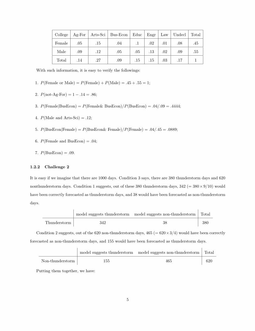
College Ag-For Arts-Sci Bus-Econ Educ Engr Law Undecl Total

Female .05 .15 .04 .1 .02 .01 .08 .45

Male .09 .12 .05 .05 .13 .02 .09 .55

Total .14 .27 .09 .15 .15 .03 .17 1

With such information, it is easy to verify the followings:

1. P (Female or Male) = P (Female) + P (Male) = .45 + .55 = 1;

2. P (not-Ag-For) = 1− .14 = .86;

3. P (Female|BusEcon) = P (Female& BusEcon)/P (BusEcon) = .04/.09 = .4444;

4. P (Male and Arts-Sci) = .12;

5. P (BusEcon|Female) = P (BusEcon& Female)/P (Female) = .04/.45 = .0889;

6. P (Female and BusEcon) = .04;

7. P (BusEcon) = .09.

1.2.2 Challenge 2

It is easy if we imagine that there are 1000 days. Condition 3 says, there are 380 thunderstorm days and 620

nonthunderstorm days. Condition 1 suggests, out of these 380 thunderstorm days, 342 (= 380×9/10) would

have been correctly forecasted as thunderstorm days, and 38 would have been forecasted as non-thunderstorm

days.

model suggests thunderstorm model suggests non-thunderstorm Total

Thunderstorm 342 38 380

Condition 2 suggests, out of the 620 non-thunderstorm days, 465 (= 620×3/4) would have been correctly

forecasted as non-thunderstorm days, and 155 would have been forecasted as thunderstorm days.

model suggests thunderstorm model suggests non-thunderstorm Total

Non-thunderstorm 155 465 620

Putting them together, we have:

5

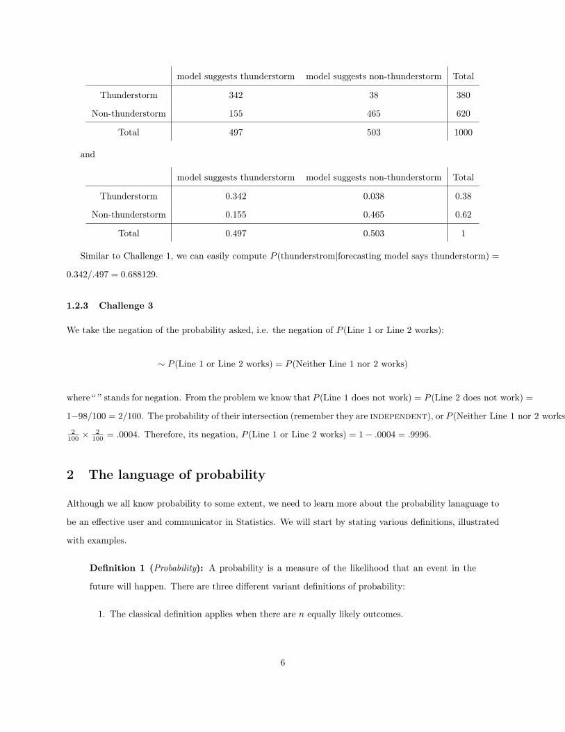
model suggests thunderstorm model suggests non-thunderstorm Total

Thunderstorm 342 38 380

Non-thunderstorm 155 465 620

Total 497 503 1000

and

model suggests thunderstorm model suggests non-thunderstorm Total

Thunderstorm 0.342 0.038 0.38

Non-thunderstorm 0.155 0.465 0.62

Total 0.497 0.503 1

Similar to Challenge 1, we can easily compute P (thunderstrom|forecasting model says thunderstorm) =

0.342/.497 = 0.688129.

1.2.3 Challenge 3

We take the negation of the probability asked, i.e. the negation of P (Line 1 or Line 2 works):

∼ P (Line 1 or Line 2 works) = P (Neither Line 1 nor 2 works)

where “ ” stands for negation. From the problem we know that P (Line 1 does not work) = P (Line 2 does not work) =

1−98/100 = 2/100. The probability of their intersection (remember they are independent), or P (Neither Line 1 nor 2 works) =

2100 ×

2100 = .0004. Therefore, its negation, P (Line 1 or Line 2 works) = 1− .0004 = .9996.

2 The language of probability

Although we all know probability to some extent, we need to learn more about the probability lanaguage to

be an effective user and communicator in Statistics. We will start by stating various definitions, illustrated

with examples.

Definition 1 (Probability): A probability is a measure of the likelihood that an event in the

future will happen. There are three different variant definitions of probability:

1. The classical definition applies when there are n equally likely outcomes.

6

2. The empirical or statistical definition applies when the number of times the event happens

is divided by the number of observations, based on data.

3. Subjective probability is based on whatever information is available, based on subjective

feelings.

In this book, we mainly deal with the empirical or statistical definition of probability.

Example 1 (Classical, and subjective probability):

1. Classical: in the tossing of a single perfectly cubical die, made of completely homogeneous

material, the equally likely events are the appearance of any of the specific number of dots

(from 1 to 6) on its upper face.

2. Subjective probability: Without using econometric/statistical models, I report that the

probability that HK’s economic growth will be 3% or above this year is 0.7. (Note that a

lot of economists report this kind of subjective probability or forecast without any serious

research – so called gut feelings.)

Example 2 (Empirical probability): Throughout her teaching career Professor Jones has awarded

186 A’s out of 1,200 students. What is the probability that a student in her section this semester

will receive an A?

This is an example of the empirical definition of probability. The probability that a randomly

selected student earned an A is

P (an A grade) =1861200

= 0.155

This number may be interpreted as “unconditional probability”. In most cases, we are interested

in the probability of earning an A for a selected student who study 10 hours or more per week.

We call this “conditional probability”.

P (A|study 10 or more hours per week)

Definition 2 (Experiment and outcome): An experiment is the observation of some activity or

the act of taking some measurement. An outcome is the particular result of an experiment.

7

Example 3 (Experiment and outcome I): A fair die is rolled once. The experiment is rolling the

one die. The possible outcomes are the numbers 1, 2, 3, 4, 5, and 6.

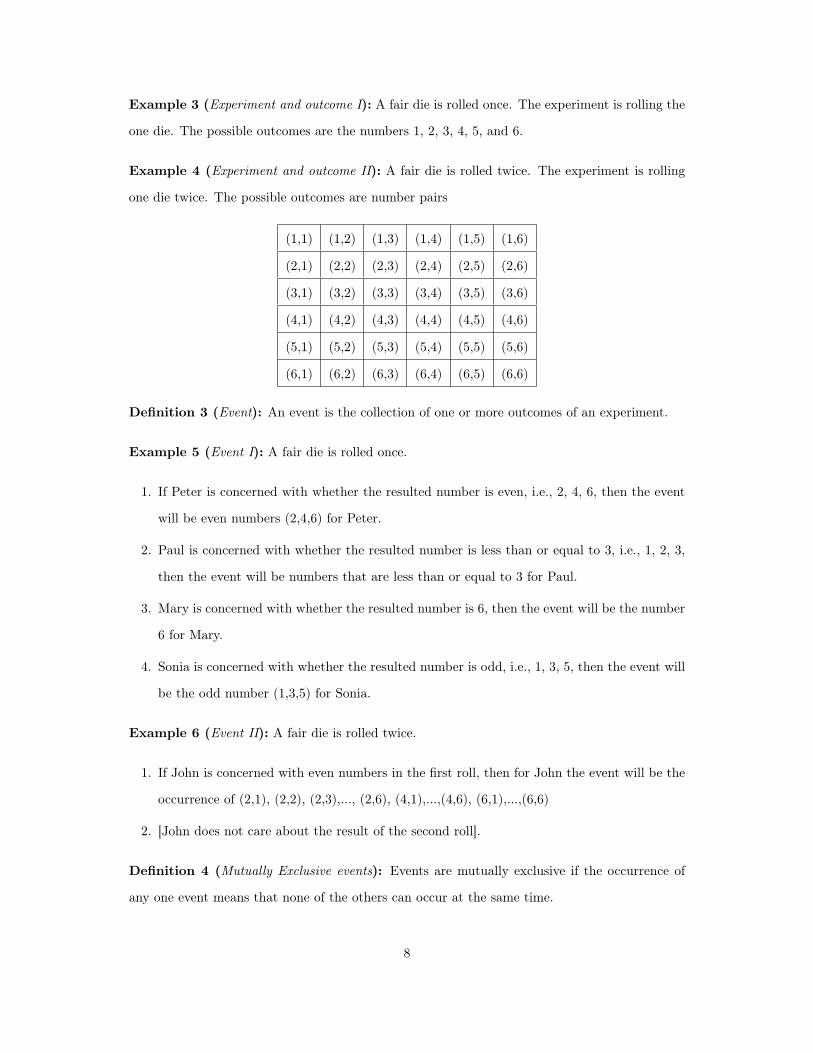
Example 4 (Experiment and outcome II): A fair die is rolled twice. The experiment is rolling

one die twice. The possible outcomes are number pairs

(1,1) (1,2) (1,3) (1,4) (1,5) (1,6)

(2,1) (2,2) (2,3) (2,4) (2,5) (2,6)

(3,1) (3,2) (3,3) (3,4) (3,5) (3,6)

(4,1) (4,2) (4,3) (4,4) (4,5) (4,6)

(5,1) (5,2) (5,3) (5,4) (5,5) (5,6)

(6,1) (6,2) (6,3) (6,4) (6,5) (6,6)

Definition 3 (Event): An event is the collection of one or more outcomes of an experiment.

Example 5 (Event I): A fair die is rolled once.

1. If Peter is concerned with whether the resulted number is even, i.e., 2, 4, 6, then the event

will be even numbers (2,4,6) for Peter.

2. Paul is concerned with whether the resulted number is less than or equal to 3, i.e., 1, 2, 3,

then the event will be numbers that are less than or equal to 3 for Paul.

3. Mary is concerned with whether the resulted number is 6, then the event will be the number

6 for Mary.

4. Sonia is concerned with whether the resulted number is odd, i.e., 1, 3, 5, then the event will

be the odd number (1,3,5) for Sonia.

Example 6 (Event II): A fair die is rolled twice.

1. If John is concerned with even numbers in the first roll, then for John the event will be the

occurrence of (2,1), (2,2), (2,3),..., (2,6), (4,1),...,(4,6), (6,1),...,(6,6)

2. [John does not care about the result of the second roll].

Definition 4 (Mutually Exclusive events): Events are mutually exclusive if the occurrence of

any one event means that none of the others can occur at the same time.

8

Example 7 (Mutually Exclusive events): A fair die is rolled once. Suppose Peter, Paul and

Mary are concerned of the following events:

1. Peter is concerned with whether the resulted number is even, i.e., 2, 4, 6.

2. Paul is concerned with whether the resulted number is less than or equal to 3, i.e., 1, 2, 3.

3. Mary is concerned with whether the resulted number is 6.

Then,

1. Peter’s event and Paul’s event are not mutually exclusive - both contains 2.

2. Peter’s event and Mary’s event are not mutually exclusive - both contains 6.

3. Paul’s event and Mary’s event are mutually exclusive - no common numbers.

Definition 5 (Exhaustive events): Events are collectively exhaustive if at least one of the events

must occur when an experiment is conducted.

Example 8 (Exhaustive events I): A fair die is rolled once. Suppose Peter, Paul and Mary are

concerned of the following events:

1. Peter is concerned with whether the resulted number is even, i.e., 2, 4, 6.

2. Paul is concerned with whether the resulted number is less than or equal to 3, i.e., 1, 2, 3.

3. Mary is concerned with whether the resulted number is 6.

Then,

1. Peter’s event and Paul’s event are not collectively exhaustive.

2. Peter’s event and Mary’s event are not collectively exhaustive.

3. Paul’s event and Mary’s event are not collectively exhaustive.

4. Peter’s event, Paul’s event and Mary’s events are not collectively exhaustive.

Example 9 (Exhaustive events II): A fair die is rolled once. Suppose Peter, Paul and Mary are

concerned of the following events:

1. Peter is concerned with whether the resulted number is 1, 2, 3.

2. Paul is concerned with whether the resulted number is 3, 4, 5.

9

3. Mary is concerned with whether the resulted number is 4, 5, 6.

Then,

1. Peter’s event and Paul’s event are not collectively exhaustive.

2. Peter’s event and Mary’s event are collectively exhaustive.

3. Paul’s event and Mary’s event are not collectively exhaustive.

4. Peter’s event, Paul’s event and Mary’s events are collectively exhaustive.

Definition 6 (Conditional Probability): A conditional probability is the probability of a par-

ticular event occurring, given that another event has occurred. The probability of the event A

given that the event B has occurred is written P (A|B).

We are gerenally more interested in conditional probability than unconditional probability. For examples,

we are more interested in the probability of getting an A grade for the student who spend more than 10

hours studying this course a week than the probability of a randomly selected student to get an A grade. So,

event A is “an A grade for the student” and event B is “the student who spend more than 10 hours studying

this course a week”. We can also be interested in the probability of of getting an A grade for the student

who is female and spend more than 10 hours studying this course a week. In this case, event A is “an A

grade for the student” and event B is “the student who is female and spend more than 10 hours studying

this course a week”.

Example 10 (Conditional probability): P(A|B)

1. A = “the Hang Seng Index goes up tomorrow”; B = ”the weather is cloudy tomorrow”.

2. A = “the stock price of HSBC in Hong Kong Stock Exchange goes up”; B = “the stock price

of HSBC ADR in New York Stock Exchange goes up the day before”.

3. A = “the stock price of a company rises today”; B = “the company repurchased its stock

yesteday”.

4. A = “the stock price of a company rises today”; B = “the company stock prices hit its

52-week high yesterday”.

5. A = “the stock price of a company is going to increase more than 10 percent tomorrow”; B

= “today is the company’s IPO day”.

10

6. A = “the stock returns of a company is higher than average”; B = “the CEO is a member of

communist party”.

7. A = “a fresh graduate has a higher salary than average”; B = “the fresh graduate has high

English proficiency than average”.

8. A = “a fresh graduate has a higher salary than average”; B = “the fresh graduate is more

good-looking than average”.

9. A = “a fresh graduate has a higher salary than average”; B = “the fresh graduate is borned

in the year of Dragon”.

10. A = “inflation goes up in the coming year”; B = “the inflation went up last year”.

11. A = “the city has a per capita GDP higher than nation’s average”; B = “the city is coastal”.

12. A = “the company is going to lay off its employees”; B = “the economy is entering a recession”.

13. A = “market price of pork is to rise”; B = “market price of beef declined”.

14. A = “the local 3-year time deposit interest rises”; B = “a new type of government bond is

issued”.

15. A = “the company files bankruptcy”; B = “the company has oustanding liabilities more than

half of its assets”.

16. A = “a student gets a lower-than-average grade”; B = “the student skips more than 30% of

the classes”.

17. A = “the restaurant serves good food”; B = “there is a long line waiting outside the restau-

rant”.

Example 11 (Change of Inflation in Hong Kong):We want to know how likely it is that the

inflation is higher than last year (event A), given that there was an increase in inflation rate last

year (event B). Consumer price data can be obtained from the website of Census and Statistics

Department of Hong Kong (http://www.censtatd.gov.hk/).

We obtained Composite Consumers’ Price Index, CPI, from 1983 to 2006. The inflation rate is

then calculated. Whether event B and event A|B occurred were calculated as follows.1

1Note that in calculation inflation rate, we often compute annual inflation. If we have to use monthly CPI to computeinflation rate, we will almost always compute it as the annual change of CPI, say, CPI in 2006 May compared to CPI 2005 May.

11

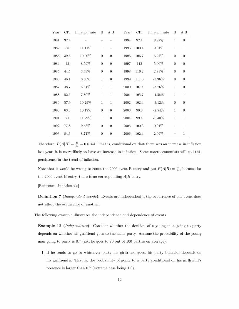
Year CPI Inflation rate B A|B Year CPI Inflation rate B A|B

1981 32.4 – – – 1994 92.1 8.87% 1 0

1982 36 11.11% 1 – 1995 100.4 9.01% 1 1

1983 39.6 10.00% 0 0 1996 106.7 6.27% 0 0

1984 43 8.59% 0 0 1997 113 5.90% 0 0

1985 44.5 3.49% 0 0 1998 116.2 2.83% 0 0

1986 46.1 3.60% 1 0 1999 111.6 -3.96% 0 0

1987 48.7 5.64% 1 1 2000 107.4 -3.76% 1 0

1988 52.5 7.80% 1 1 2001 105.7 -1.58% 1 1

1989 57.9 10.29% 1 1 2002 102.4 -3.12% 0 0

1990 63.8 10.19% 0 0 2003 99.8 -2.54% 1 0

1991 71 11.29% 1 0 2004 99.4 -0.40% 1 1

1992 77.8 9.58% 0 0 2005 100.3 0.91% 1 1

1993 84.6 8.74% 0 0 2006 102.4 2.09% – 1

Therefore, P (A|B) = 813 = 0.6154. That is, conditional on that there was an increase in inflation

last year, it is more likely to have an increase in inflation. Some macroeconomists will call this

persistence in the trend of inflation.

Note that it would be wrong to count the 2006 event B entry and put P (A|B) = 814 , because for

the 2006 event B entry, there is no corresponding A|B entry.

[Reference: inflation.xls]

Definition 7 (Independent events): Events are independent if the occurrence of one event does

not affect the occurrence of another.

The following example illustrates the independence and dependence of events.

Example 12 (Independence): Consider whether the decision of a young man going to party

depends on whether his girlfriend goes to the same party. Assume the probability of the young

man going to party is 0.7 (i.e., he goes to 70 out of 100 parties on average).

1. If he tends to go to whichever party his girlfriend goes, his party behavior depends on

his girlfriend’s. That is, the probability of going to a party conditional on his girlfriend’s

presence is larger than 0.7 (extreme case being 1.0).

12

2. If he tends to avoid going to whichever party his girlfriend goes, his party behavior also

depends on his girlfriend’s. That is, the probability of going to a party conditional on his

girlfriend’s presence is less than 0.7 (extreme case being 0.0).

3. If in making the party decision, he never considers whether his girlfriend is going to a party,

his party behavior does not depends on his girlfriend’s. That means, the probability of going

to a party conditional on his girlfriend’s presence is 0.7.

Let’s formalize the above discussion in probability terms. Suppose we consider the following two

events:

1. Event A: a young man goes to a party.

2. Event B: his girlfriend goes to the same party.

Assume P(A) =0.7. His party behavior does not depend on his girlfriend’s only if P (A|B) =

P (A) = 0.7. And, event A is said to be independent of event B.

1. P (the young man and his girlfriends shows up in a party) = P (A&B) = P (B) ∗ P (A|B).

2. If he always goes to whichever party his girlfriend goes, P (A|B) = 1. Hence, P (A&B) =

P (B) ∗ P (A|B) = P (B).

3. If he always avoid to whichever party his girlfriend goes, P (A|B) = 0. Hence, P (A&B) =

P (B) ∗ P (A|B) = 0.

4. If in making the party decision, he never considers whether his girlfriend is going to a party,

P (A|B) = 0.7. Hence, P (A&B) = P (B) ∗ P (A|B) = P (B) ∗ P (A) = 0.7.

Here are implications of independent events.

Theorem 1 (Independence):

1. Event A is independent of B if P (A|B) = P (A)

2. Event B is independent of A if P (B|A) = P (B)

3. P (A|B) = P (A) ⇒ P (A&B) = P (B|A)× P (A) = P (B)× P (A)

4. P (B|A) = P (B) ⇒ P (A&B) = P (A|B)× P (B) = P (A)× P (B)

5. Thus, if P (A&B) = P (B)×P (A), we must have either P (A|B) = P (A) or P (B|A) = P (B).

13

Example 13 (Independence): A fair die is rolled twice. John and Sarah are concerned of the

following events.

1. John is concerned with whether the resulted number of first roll is even, i.e., 2, 4, 6.

2. Sarah is concerned with whether the resulted number of second roll is even, i.e., 2, 4, 6.

The following events are independent:

1. John’s event and Sarah’s event are independent, i.e., P (John & Sarah) = P (John) ×

P (Sarah).

Theorem 2 (Special rule of addition for mutually exclusive events): If two events A and B

are mutually exclusive, the probability of A or B occurring equals the sum of their respective

probabilities:

P (A or B) = P (A) + P (B)

Example 14 (Special rule of addition for mutually exclusive events): There was a plunge for

most of the Shanghai A-share stocks on Jun 29th, 2007 (source: Yahoo! Finance):

Performance on Jun 29th Number of the stocks

Rise 106

Even 3

Drop 656

Closed 61

Total 826

We randomly draw one from all the Shanghai A-shares stocks,

1. If A is the event that the stock rose, then P (A) = 106/826 = .1283.

2. If B is the event that the stock price did not change, then P (B) = (3 + 61)/826 = .0775.

3. The probability that a randomly chosen stock did not fell is:

P (A or B) = P (A) + P (B) = .1283 + .0775 = .2058.

The complement rule is used to determine the probability of an event occurring by subtracting the

probability of the event not occurring from 1.

14

Theorem 3 (The probability of a complement – The Complement Rule): If P (A) is the proba-

bility of event A and P (∼ A) is probability of the complement of A, we have

P (A) + P (∼ A) = 1 because A and ∼ A are mutually exclusive.

⇒ P (A) = 1− P (∼ A).

where A reads “not A”.

Complement rule is extremely useful when one probability is very difficult to compute but its complment

is easy.

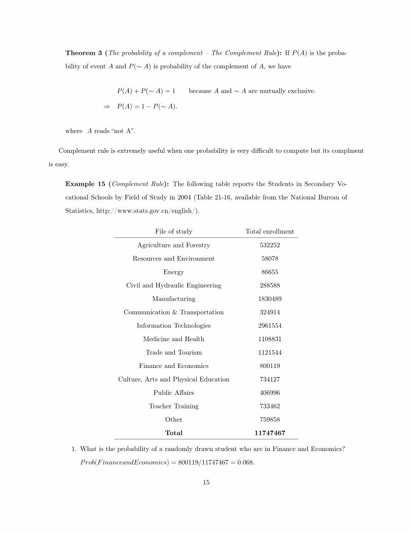
Example 15 (Complement Rule): The following table reports the Students in Secondary Vo-

cational Schools by Field of Study in 2004 (Table 21-16, available from the National Bureau of

Statistics, http://www.stats.gov.cn/english/).

File of study Total enrollment

Agriculture and Forestry 532252

Resources and Environment 58078

Energy 86655

Civil and Hydraulic Engineering 288588

Manufacturing 1830489

Communication & Transportation 324914

Information Technologies 2961554

Medicine and Health 1108831

Trade and Tourism 1121544

Finance and Economics 800119

Culture, Arts and Physical Education 734127

Public Affairs 406996

Teacher Training 733462

Other 759858

Total 11747467

1. What is the probability of a randomly drawn student who are in Finance and Economics?

Prob(FinanceandEconomics) = 800119/11747467 = 0.068.

15

2. What is the probability of a randomly drawn student who are in one of the following

fields: Agriculture and Forestry, Resources and Environment, Energy, Civil and Hydraulic

Engineering, Manufacturing, Communication & Transportation, Information Technologies,

Medicine and Health, Trade and Tourism, Finance and Economics, Culture, Arts and Phys-

ical Education, Public Affairs, and Teacher Training?

Prob(inonofthefields) = 1− Prob(other) = 1− 0.065 = 0.935.

Note how the complement rule has helped simplify greatly the calculation of the probability.

Theorem 4 (The General Rule of Addition): If A and B are two events that are not mutually

exclusive, then P(A or B) is given by the following formula:

P (A or B) = P (A) + P (B)− P (A and B)

Example 16 (The General Rule of Addition): The following table reports the Number of Post-

graduate Students by Field of Study in China (2004). (Table 21-9, available from the National

Bureau of Statistics, http://www.stats.gov.cn/english/).

Field Doctor’s Degree Master’s Degree Total Enrollment

Philosophy 2143 7523 9666

Economics 8564 33861 42425

Law 6515 49060 55575

Education 2510 20302 22812

Literature 6434 51155 57589

History 2771 8548 11319

Science 28769 73612 102381

Engineering 69315 248748 318063

Agricultrue 6112 22818 28930

Medicine 17771 64088 81859

Military 109 318 427

Management 14597 74253 88850

Total 165610 654286 819896

1. If a postgraduate student is selected at random, what is the probability that the student

16

was studying in the field of Economics (event E), studying for a doctor’s degree (event D),

and studying a doctor’s degree in the field of Economics (event D&E)?

(a) Prob(studying in the field of Economics) = Prob(E) = 0.052.

(b) Prob(studying for a doctor′s degree) = Prob(D) = 0.202.

(c) Prob(Studying a doctor′s degree in the field of Economics) = Prob(D&E) = 0.010.

2. If a postgraduate student is selected at random, what is the probability that the student

was studying in the field of Economics or studying for a doctor’s degree?

Prob(E or D) = Prob(E) + Prob(D)− Prob(D&E) = 0.052 + 0.202− 0.010 = 0.244.

Example 17 (The General Rule of Addition): In a sample of 500 students, 320 said they had a

stereo, 175 had a TV, and 100 said they had both.

1. If a student is selected at random, what is the probability that the student has only a stereo,

only a TV, and both a stereo and TV?

Note that P(student as only a stereo) = P(student has a stereo) - P(student has both a stereo

and TV), and P(student has only a TV) = P(student has a TV)- P(student has both a stereo

and TV). We only need to find the quantities in steps.

(a) P(student has a stereo) = 320/500 = .64.

(b) P(student has a TV) = 175/500 = .35.

(c) P(student has both a stereo and TV) = 100/500 = .20.

(d) P(student as only a stereo) = 220/500 = .44.

(e) P(student has only a TV) = 75/500 = .15.

2. If a student is selected at random, what is the probability that the student has either a

stereo or a TV in his or her room?

P (either S or T ) = P (only S) + P (only T )

= [P (S)− P (S and T )] + [P (T )− P (S and T )]

= .64− .20 + .35− .20 = .59.

Definition 8 (Joint Probability): A joint probability measures the likelihood that two or more

events will happen concurrently.

17

An example would be the event that a student has both a stereo and TV in his or her dorm room. Another

example is the joint probability of getting 5 and 6 from a throw of dice. Note that because the two outcomes

are mutually exclusive, P(dice=5, and dice=6) =0.

The special rule of multiplication requires that two events A and B are independent. Recall that two

events A and B are independent if the occurrence of one has no effect on the probability of the occurrence

of the other. Thus,

Theorem 5 (Special Rule of Multiplication): When the two events A and B are independent,

P (A and B) = P (A)P (B)

Example 18 (Special rule of multiplication): Chris owns two stocks, IBM and General Electric

(GE). The probability that IBM stock will increase in value next year is .5 and the probability

that GE stock will increase in value next year is .7. Assume the two stocks are independent.

What is the probability that both stocks will increase in value next year?

Using the Special Rule of Multiplication, we have

P (IBM and GE) = (.5)(.7) = .35.

Note that stock prices are generally not independent. In the study of finance, the fluctuation (or risk)

of stock prices are decomposed into to components: Idiosyncratic risk and systematic risk (or market risk).

It is said that idiosyncratic risk may be reduced by holding a portfolio of assets but systematic risk may

not reduced through diversification. For instance, when the US Federal Reserve Board raises its overnight

interest rate, all stocks are affected. Thus, all stock prices appear dependent on each other to some extent.

The general rule of multiplication is used to find the joint probability that two events will occur.

Definition 9 (General Multiplication Rule): For two events A and B, the joint probability that

both events will happen is found by multiplying the probability that event A will happen by the

conditional probability of B given that A has occurred.

That is, the joint probability, P(A and B) is given by the following formula:

P (A and B) = P (A)P (B|A)

18

or

P (A and B) = P (B)P (A|B)

For example, P (test says girl and girl) = P (girls)×P (test says girls|girls), and P (test says boy and boy) =

P (boys)× P (test says boys|boys).

Example 19 (General Multiplication Rule): The Dean of the School of Business at Owens

University collected the following information about undergraduate students in her college:

MAJOR Male Female Total

Accounting 170 110 280

Finance 120 100 220

Marketing 160 70 230

Management 150 120 270

Total 600 400 1000

1. If a student is selected at random, what is the probability that the student is a female (F)

accounting major (A)?

P(A and F) = 110/1000.

2. Given that the student is a female, what is the probability that she is an accounting major?

Approach 1: P (A|F ) = P (A&F )/P (F ) = [110/1000]/[400/1000] = .275

Approach 2: P (A|F ) = 110/400 = .275

3 Tree Diagrams

Definition 10 (Tree Diagrams): A branching diagram that shows all possible combinations or

outcomes.

A tree diagram is useful for portraying conditional and joint probabilities. It is particularly useful for

analyzing business decisions involving several stages.

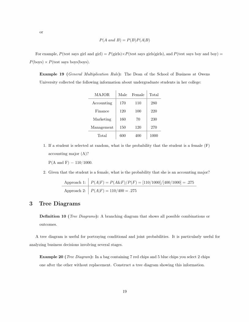
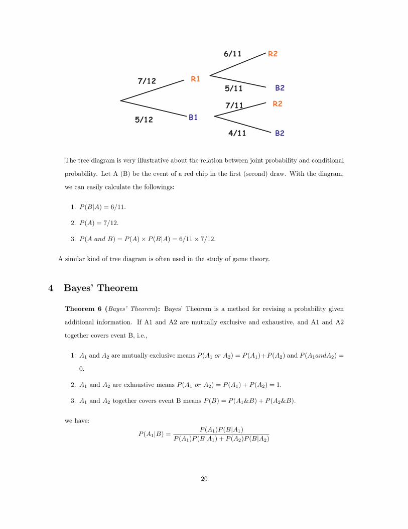
Example 20 (Tree Diagram): In a bag containing 7 red chips and 5 blue chips you select 2 chips

one after the other without replacement. Construct a tree diagram showing this information.

19

R1

B1

R2

B2

R2

B2

7/12

5/12

6/11

5/11

7/11

4/11

The tree diagram is very illustrative about the relation between joint probability and conditional

probability. Let A (B) be the event of a red chip in the first (second) draw. With the diagram,

we can easily calculate the followings:

1. P (B|A) = 6/11.

2. P (A) = 7/12.

3. P (A and B) = P (A)× P (B|A) = 6/11× 7/12.

A similar kind of tree diagram is often used in the study of game theory.

4 Bayes’ Theorem

Theorem 6 (Bayes’ Theorem): Bayes’ Theorem is a method for revising a probability given

additional information. If A1 and A2 are mutually exclusive and exhaustive, and A1 and A2

together covers event B, i.e.,

1. A1 and A2 are mutually exclusive means P (A1 or A2) = P (A1)+P (A2) and P (A1andA2) =

0.

2. A1 and A2 are exhaustive means P (A1 or A2) = P (A1) + P (A2) = 1.

3. A1 and A2 together covers event B means P (B) = P (A1&B) + P (A2&B).

we have:

P (A1|B) =P (A1)P (B|A1)

P (A1)P (B|A1) + P (A2)P (B|A2)

20

Bayes’ Theorem is an essential tool to understand options and real options in finance. Bayes’ Theorem can

be derived based on simple manipulation of the general multiplication rule.

P (A1|B) = P (A1&B)/P (B)

= [P (A1)P (B|A1)]/P (B)

= [P (A1)P (B|A1)]/[P (A1&B) + P (A2&B)]

= [P (A1)P (B|A1)]/[P (A1)P (B|A1) + P (A2)P (B|A2)

Example 21 (Bayes’ Theorem): Duff Cola Company recently received several complaints that

their bottles are under-filled. A complaint was received today but the production manager is

unable to identify which of the two Springfield plants (A or B) filled this bottle. The following

table summarizes the Duff production experience.

% of Total Production % of under-filled bottles

A 55 3

B 45 4

What is the probability that the under-filled bottle came from plant A?

P (A|U) =P (A)P (U |A)

P (A)P (U |A) + P (B)P (U |B)

=.55(.03)

.55(.03) + .45(.04)

= .4783

The likelihood the bottle was filled in Plant A is reduced from .55 to .4783. Without the infor-

mation about U, the manager will say the under-filled bottle is likely from plant A. With the

additional information about U, the manager will say the under-filled bottle is likely from plant

B.

Example 22 (Bayes’ Theorem II): There are in all 31 provinces, municipalities, and autonomous

regions in Mainland China, among which 11 are coastal2. According to the National Statistics

Bureau, in 2005, national average per capita GDP was RMB 14040. There were 19 regions with2The coastal ones are: Liaoning, Hebei, Tianjing, Shandong, Jiangsu, Shanghai, Zhejiang, Fujian, Guangdong, Hainan and

Guangxi.

21

below average per capita GDP, including 16 non-coastal ones. (Table 3-1 and 3-9, available from

the National Bureau of Statistics, http://www.stats.gov.cn/english/).

Suppose we want to study the imbalance of development between the east and west of China,

and we want to know the proportion or probability of coastal regions that had a higher than

average per capita GDP.

It is often convenient to mark the events with letters.

C: the region is a coastal one;

A: the region had above average per capita GDP in 2005.

Then we know, P (C) = 1131 , P (∼ A) = 19

31 , P (∼ C | ∼ A) = 1619 . The probability we want to know

is P (C |A) and by Bayes’ Theorem:

P (C |A) =P (C&A)

P (A)

=P (A | C)× P (C)

P (A | C)× P (C) + P (A | ∼ C)× P (∼ C)

Using the complementary rule, we can have all the values in the above formula and just simply

plug them in. We have P (C |A) = 811 = .7273.

Example 23 (Bayes’ Theorem III): Mr. Zhou has been keeping a stock for a very long period

of time. Based on his observations, he finds that most of the time his stock moves together with

the market index. To be specific, when his stock rises, the market index rises 75% of the times;

while when his stock drops, the market drops 95% of the times. And we know the chance to close

even (i.e., unchanged) is rare.

Tomorrow is the day on which the financial reports of the company to be announced. Mr. Zhou

is quite anxious about the report. Usually whenever the financial reports reveal a positive net

income, the company’s stock will rise 70% of the time; whenever the net income revealed is

negative, the company’s stock has 80% of chance to drop.

Mr. Zhou analyzed the past performance of the company and believes the financial reports

tomorrow will 60% likely release a positive net income. Mr. Zhou now wants to know what is

the probability for his stock to rise, given the market is to rise.

To help Mr. Zhou, we first label some letters for different events.

22

Event Letter Probability

The market index rises. R unknown yet

Mr. Stoke’s stock rises. M unknown yet

Positive net income tomorrow. N P (N) = 60%

What Mr. Zhou is interested in is P (M |R). Although we currently knows the probability for the

rumour to be true only, we know quite a lot about other conditional probabilities: P (M |N) =

70%, P (M | ∼ N) = 1− 80% = 20%; P (R|M) = 75%, P (R| ∼ M) = 1− 95% = 5%.

This information helps us to first compute P (M):

P (M) = P (M |N)× P (N) + P (M | ∼ N)× P (∼ N)

= 70%× 60% + 20%× (1− 60%)

= 50%

By Bayes’ Theorem:

P (M |R) =P (R |M)× P (M)

P (R |M)× P (M) + P (R | ∼ M)× P (∼ M)

=75%× 50%

75%× 50% + 5%× (1− 50%)

= 93.75%

This result shows that Mr. Zhou’s stock will probably performs well as long as the market

does well tomorrow. In another word, the financial reports to be revealed tomorrow are of less

importance (we assume all the events mentioned are independent).

5 Counting rules

5.1 Probabilities for n Dice

Suppose we roll n regular balanced six-sided dice. If the event X is the sum of the n values which appear,

what are the probabilities associated for each value of X, for the possible values X = n, ..., 6n?

In the case n = 1, the possible outcomes are {1, 2, 3, 4, 5, 6}. The probabilities of these individual outcomes

are all 1/6.

23

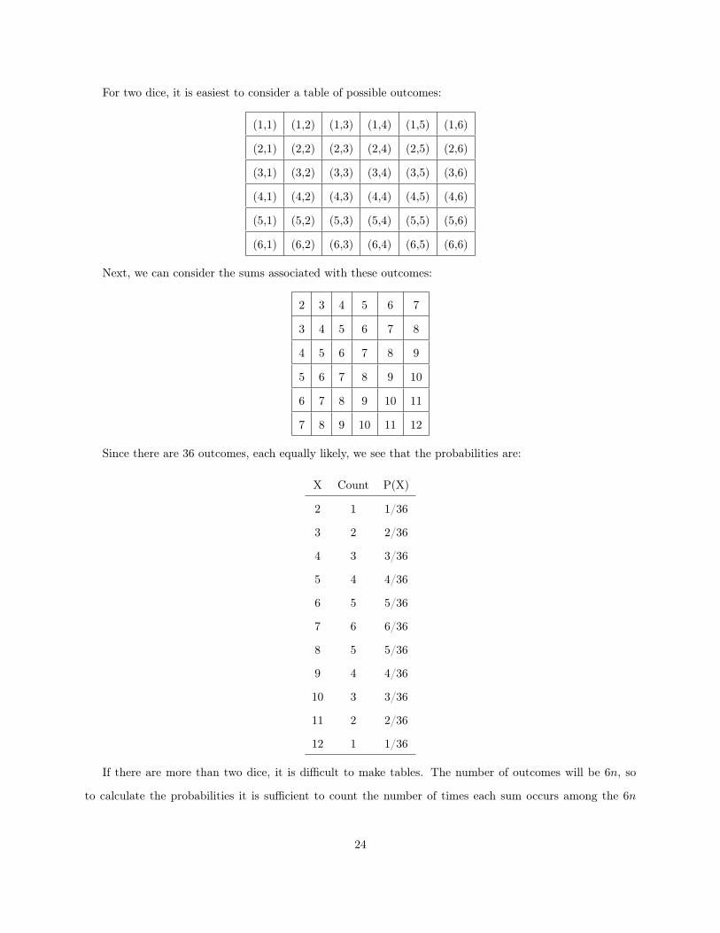
For two dice, it is easiest to consider a table of possible outcomes:

(1,1) (1,2) (1,3) (1,4) (1,5) (1,6)

(2,1) (2,2) (2,3) (2,4) (2,5) (2,6)

(3,1) (3,2) (3,3) (3,4) (3,5) (3,6)

(4,1) (4,2) (4,3) (4,4) (4,5) (4,6)

(5,1) (5,2) (5,3) (5,4) (5,5) (5,6)

(6,1) (6,2) (6,3) (6,4) (6,5) (6,6)

Next, we can consider the sums associated with these outcomes:

2 3 4 5 6 7

3 4 5 6 7 8

4 5 6 7 8 9

5 6 7 8 9 10

6 7 8 9 10 11

7 8 9 10 11 12

Since there are 36 outcomes, each equally likely, we see that the probabilities are:

X Count P(X)

2 1 1/36

3 2 2/36

4 3 3/36

5 4 4/36

6 5 5/36

7 6 6/36

8 5 5/36

9 4 4/36

10 3 3/36

11 2 2/36

12 1 1/36

If there are more than two dice, it is difficult to make tables. The number of outcomes will be 6n, so

to calculate the probabilities it is sufficient to count the number of times each sum occurs among the 6n

24

possible outcomes. This is easily done by considering the generating function for the number of times each

sum appears:

f(x) = (x + x2 + x3 + x4 + x5 + x6)n

In our earlier example, n = 2:

(x + x2 + x3 + x4 + x5 + x6)2

= x2 + 2x3 + 3x4 + 4x5 + 5x6 + 6x7 + 5x8 + 4x9 + 3x10 + 2x11 + x12

The coefficient of x3 is number of times the sum of 3 occurs.

5.2 Multiplication formula

The multiplication formula indicates that if there are m ways of doing one thing and n ways of doing another

thing, there are m× n ways of doing both.

Example 24 (multiplication formula): Dr. Delong has 10 shirts and 8 ties. How many shirt

and tie outfits does he have?

Applying the multiplication formula directly, Dr. Delong have (10)(8) = 80 outfits.

Definition 11 (Permutation): A permutation is any arrangement of r objects selected from n

possible objects.

nPr =n!

(n− r)!

where n! = n× (n− 1)× (n− 2)× ...× 2× 1.

Definition 12 (Combination): A combination is the number of ways to choose r objects from a

group of n objects without regard to order.

nCr =n!

r!(n− r)!

Example 25 (Permutation and Combination): There are 12 players on the Carolina Forest High

School basketball team. Coach Thompson must pick five players among the twelve on the team

to comprise the starting lineup. How many different groups are possible? Since the order of

25

players is not a concern, we can use the combination formula directly and get

12C5 =12!

5!(12− 5)!= 792

Suppose that in addition to selecting the group, he must also rank each of the players in that

starting lineup according to their ability. Since the order of players is a concern, we will use the

permutation formula to get

12P5 =12!

(12− 5)!= 95, 040

26

Problem sets

We have tried to include some of the most important examples in the text. To get a good understand of

the concepts, it is most useful to re-do the examples and simulations in the text. Work on the following

problems only if you need extra practice or if your instructor assigns them as an assignment. Of course, the

more you work on these problems, the more you learn.

1. Write five examples of conditional probability.

2. Write an example to illustrate the concept of independence.

27