SPE 79678

A Strategy for Rapid Quantification of Uncertainty in Reservoir Performance Prediction Sam Subbey, SPE, Mike Christie, SPE, Heriot-Watt University, Edinburgh, UK, Malcolm Sambridge, Australian National University, Australia

Copyright 2003, Society of Petroleum Engineers Inc. This paper was prepared for presentation at the SPE Reservoir Simulation Symposium held in Houston, Texas, U.S.A., 3–5 February 2003. This paper was selected for presentation by an SPE Program Committee following review of information contained in an abstract submitted by the author(s). Contents of the paper, as presented, have not been reviewed by the Society of Petroleum Engineers and are subject to correction by the author(s). The material, as presented, does not necessarily reflect any position of the Society of Petroleum Engineers, its officers, or members. Papers presented at SPE meetings are subject to publication review by Editorial Committees of the Society of Petroleum Engineers. Electronic reproduction, distribution, or storage of any part of this paper for commercial purposes without the written consent of the Society of Petroleum Engineers is prohibited. Permission to reproduce in print is restricted to an abstract of not more than 300 words; illustrations may not be copied. The abstract must contain conspicuous acknowledgment of where and by whom the paper was presented. Write Librarian, SPE, P.O. Box 833836, Richardson, TX 75083-3836, U.S.A., fax 01-972-952-9435.

Abstract This paper will describe a strategy for rapid quantification of uncertainty in reservoir performance prediction. The strategy is based on a combination of streamline and conventional finite difference simulators.

Our uncertainty framework uses the Neighbourhood Approximation algorithm to generate an ensemble of history match models, and has been described previously. A speedup in generating the misfit surface is essential since effective quantification of uncertainty can require thousands of reservoir model runs.

Our speedup strategy for quantifying uncertainty in performance prediction involves using an approximate streamline simulator to rapidly explore the parameter space to identify good history matching regions, and to generate an approximate misfit surface. We then switch to a conventional, finite difference simulator, and selectively explore the identified parameter space regions.

This paper will show results from a parallel version of the Neighbourhood Approximation algorithm on a Linux cluster, demonstrating the advantages of perfect parallelism. We show how it is possible to sample from the posterior probability distribution both to assess accuracy of the approximate misfit surface, and also to generate automatic history match models.

Introduction Petroleum reservoir data is inherently uncertain. The field information is usually sparse and noisy. Part of the data is obtained from cores collected at a finite set of wells. The data may also consist of time averaged responses over large scales or derived from an incomplete knowledge of the subsurface geology. The standard procedure for reducing the uncertainty is by constraining the model to data representative of the chosen recovery scheme, i.e., dynamic data, in the form of oil,

water and gas production rates, as well as pressure. In contrast to the static data (e.g., geometry and geology) obtained prior to the inception of production, these data are a direct measure of the reservoir response to the recovery process in application. The use of dynamic data in constraining the reservoir model is therefore a sound paradigm. This process of incorporating dynamic data in the generation of reservoir models is known as history matching.

The history-matching problem involves determining a set of parameters such that the model output is as close to the history data as possible. What makes history matching a daunting task is the usually high dimensionality of the model parameters, and the non-linear relationship between the parameters and the model output. A second consideration is that the history-matching problem belongs to a class of mathematical problems, which are referred to as inverse and ill-posed [1]. The history match is therefore non-unique, i.e.; more than one combination of the reservoir model input parameters match the observed production data. Consequently predicting model performance is also uncertain, and this uncertainty must be quantified. The only way to quantify uncertainty in reservoir performance requires the generation of multiple model realizations, which are constrained by the dynamic data. For problems with high input-output dimensions, each run of the simulator can be very expensive in CPU time. A single run of the model can take several minutes for a relatively coarse grid to several hours for a fine grid.

The fundamental task is how to rapidly generate multiple realizations by exhaustive exploration of parameter space. This is directly tied in with a second consideration, which is the need to restrict the range of investigation for the unknown parameters, thus preventing the algorithm from searching for physically unrealistic solutions. Since realistic uncertainty quantification depends on the quality of the ensemble of solutions generated, the above considerations are imperative for quantifying uncertainty in reservoir performance prediction Two distinct approaches to exploring model parameter space have been identified in the literature namely, deterministic [2, 3, 4, 5] and stochastic [6, 7, 8] methods.

The underlying assumption for all gradient type algorithms is the existence of a (unique) global optimum set of parameters. By moving along gradients in the misfit surface, one aims at finding this global optimum. The search process requires deriving sensitivity coefficients. This involves calculating the gradient of the performance index (objective function). For high dimensional parameter space problems,

2 S. SUBBEY, M.CHRISTIE, M. SAMBRIDGE SPE 79678

calculating sensitivity coefficients can be prohibitively expensive. Steepest descent and conjugate gradients methods are one of the earliest gradient-based algorithms reported in the literature [9]. By using optimal control theory with first-derivative minimization methods (steepest descent and conjugate gradient methods), [10] and [9] provided an attractive approach to history matching that involved efficient evaluation of the performance index, regardless of the dimensionality of the problem. However, the steepest descent method is known to progress slowly in the vicinity of the minimum [10]. Further, except in cases where the objective function is quadratic or nearly quadratic, conjugate gradient methods have been shown to be (theoretically [11], and in numerical experimentation [12]) inferior to variable metric (or quasi-Newton methods) methods. Hence other authors (see e.g., [13, 14]) have used a combination of optimal control theory and quasi-Newton methods as an approach to history matching.

More recently, the most efficient deterministic methods reported in the literature involve the steepest descent, Gauss-Newton and Levenberg-Marquardt algorithms, where deriving the sensitivity parameters involves differentiation of the mathematical model with respect to the model parameters. These sensitivity parameters are then used to construct a Hessian matrix whose inverse gives a good approximation to the covariance matrix that enters into the model misfit calculation [3, 4,].

Recent commercial aids to history matching have been based on gradient techniques. The sole aim is to generate a single history matched model, which is constrained by the dynamic data. Whereas the codes automatically generate a history-matched model, they do not guarantee that it is the correct global optimum solution. We recall that several local mimina of the objective function may exist, and the risk of getting trapped in a local minimum is a realistic scenario. A further consideration is the fact that seeking a single solution to an inverse and ill-posed problem is unsound, considering the generic properties of this class of problems, see [1]. Finally, gradient-type methods for history matching do not allow quantification of uncertainty, and therefore ignore the fact that the dynamic data is uncertain. The above realizations have led to a new approach to the problem of history matching namely, the use of stochastic methods.

Stochastic approaches to history matching recognize that the dynamic data is a realization of a stochastic process [15]. Prominent among the stochastic methods are those based on simulated annealing and genetic algorithms, see e.g., [6, 7, 16, 17]. Stochastic global optimization techniques provide a framework that allows for an intelligent evolution of the algorithm to a global optimum value of the objective function. Both methods, i.e., simulated annealing and genetic algorithms require a problem-specific way of generating a new solution from an old one, e.g., for genetic algorithm through mutation.

Simulated annealing is simpler than genetic algorithms because it only examines one point in the search space at a time, while genetic algorithms maintain a population of points. Simulated annealing does not provide for assortment, which might mix information from potential solutions to produce better ones. See [16] for a detailed discussion on the application of simulated annealing and other

global optimizers to reservoir description. In general, stochastic algorithms have slower convergence rates, compared to deterministic algorithms. Even though several realizations of the model are generated at each stage, there is limited and selective passing of information from one iterative stage to another. The amount of information to be passed on depends on tuning parameters, (e. g., for genetic algorithms, selection, crossover and mutation parameters [18, 19], and for simulated annealing, the temperature parameter [20]), which must be predetermined. This paper will present an algorithm, which makes judicious use of all information obtained in every iterative stage, in sampling the parameter space.

The Neighbourhood Approximation (NA) sampling algorithm is a stochastic algorithm, which falls in the same category as genetic algorithms and simulated annealing. This paper presents the use of the algorithm in generating multiple history-matching models. The Neighbourhood Approximation algorithm firstly identifies all good history matching regions of the parameter space. It then generates an ensemble of models that preferentially sample these regions of the model parameter-space in a guided way, by using all information obtained about the model space. This approach overcomes one of the principal weaknesses of stochastic algorithms namely, slow convergence. It uses Voronoi cells to represent the parameter space.

Voronoi cells and the Neighbourhood Approximation algorithm Given n points in a plane, their Voronoi diagram divides the plane according to the nearest neighbour rule namely, each point is associated with the region of the plane closest to it. The distance metric is usually Euclidean, and each Voronoi polygon in the Voronoi diagram is defined by a generator point and a nearest neighbour region, see Figure 1 below.

Figure 1 Random points in a 2D space

Voronoi cells possess very attractive geometrical and computational properties, see [21]. Figure 2.a. shows the Voronoi diagram for 100 points in space. As new points are added, the Voronoi diagram is updated based on the nearest neighbour rule. Figure 2.b. shows the updated diagram when 200 new points are added to the plane (Observe rectangular region ABCD). Thus Voronoi cells are unique (non-overlapping), space filling, and have size (volume, area) inversely proportional to the density of the generating point.

The Neighbourhood Approximation (NA) algorithm was originally developed to solve an inverse problem in earthquake seismology [19]. It differs from other stochastic algorithms in the following way. Rather than seeking a global

SPE 79678 A STRATEGY FOR RAPID QUANTIFICATION OF UNCERTAINTY IN RESERVOIR PERFORMANCE PREDICTION 3

optimal, the objective is to generate an ensemble of data-fitting models. The algorithm works by first, representing the parameter space with Voronoi cells. By constructing an approximate misfit surface for which the forward problem has been solved, the algorithm samples the parameter space by doing non-linear interpolation in multidimensional space, exploiting the neighbourhood property of the Voronoi cells. The sampling is done in a guided way such that new realizations of the model are concentrated in regions of parameter space that give good fit to the observed data. See [19] for detailed description of the algorithm, and [22, 23] for an earlier application in petroleum engineering.

a. 100 points b. 300 points

Figure 2 Updating Voronoi cells

Figure 3 Schematic diagram of NA– Gibbs Sampler

Specifically, the NA-algorithm generates multiple data-fitting models in parameter space in the following way. Firstly an initial set of ns models are randomly generated. In the second step, the nr models with the lowest misfit models among the most recently generated ns models (including all previously generated models) are determined. Finally, new ns models are generated by uniform random walk in the Voronoi cell of each of the nr chosen models. The algorithm returns to the second step and the process is repeated. At each iteration nr cells are resampled and in each Voronoi cell, ns/nr models are generated. The performance of the algorithm depends on the ratio ns/nr, rather than on the individual tuning parameters.

We note that at any stage of the sampling procedure, selective sampling of good data-fit regions is achieved by exploiting information about all previously generated models.

In this way it attempts to overcome a main concern of stochastic sampling - poor convergence.

Generating new ns/nr cells within a Voronoi cell is accomplished by a Gibbs sampler [24]. Figure 3 shows a 2-dimensional example. To generate a new model in cell A, we set the conditional probability density function outside Voronoi cell A to be zero. A new x-axis component xaa is obtained by a uniform random perturbation from point xa. This perturbation is restricted to lie between x1 and x2. From (xaa , ya), we generate a new y-axis component by a uniform random perturbation, restricted to lie between y1 and y2, to arrive at (xaa , yaa). This approach extends directly to multidimensional space. Thus for an m-dimensional space problem, one generates m random walks, one per axis, resulting in an m-dimensional polygon. See [19] for details.

Parallel computing Earlier use of parallel machines in the industry dealt mainly with internal parallelization. This involved developing parallel versions of the flow equations, and distributing the computation over multiple processors, such as in [25, 26]. Targeted were the computationally intensive and CPU time consuming parts of the flow equations. At present some commercial aids to history matching based on internal Parallelization, exist on the market.

More recently, external parallelization has also been reported in the literature as a means of gaining speed-up in history matching. This involves running a code that is built to run serially, over several workstations. This type of parallelization allows the simulation of multiple input files at the same time, and takes advantage of parallel computers and a network of workstations, without modification of existing serial codes. Application of external parallelization using PVM (Parallel Virtual Machines) has been reported in the literature, see [27], [28] and [29], with interesting results.

The shift of emphasis from internal to external parrallelization can be attributed, in part, to the increasing availability of computational power. The aim of internal parallelization has been to cut down on walltime. However, the remarkable development in computational power means that we are able to achieve considerable reduction in CPU time, without the need for parallelization. This development has led to lower cost per CPU time.

Probably a second reason for the shift in emphasis can be attributed to the increasing use of stochastic algorithms in reservoir simulation and characterization. Stochastic algorithms for history matching seem to benefit most from parallel computation since the history matching process involves running multiple independent forward simulations, see e.g., [30 and 31].

This paper will show results from a parallelized version of the Neighbourhood Approximation algorithm on a Linux cluster using the MPI (Message-Passing Interface) standard. We shall present results of the parallel NA algorithm on a cluster of 32 IBM xSeries 330 dual processor 1266MHz PIII servers. Results presented in this paper will demonstrate the advantages of perfect parallelism.

4 S. SUBBEY, M.CHRISTIE, M. SAMBRIDGE SPE 79678

Speedup strategy Appraising the ensemble Sampling from the posterior As pointed out in the introduction, history matching is time

consuming, and there is a need to restrict the range of investigation for the unknown parameters. Doing this prevents the algorithm from searching for physically unrealistic solutions, and much CPU time can be saved. We recall however, that realistic uncertainty quantification depends on the quality of the ensemble of solutions generated. Hence even though restricting the range of parameters will save CPU time, it is imperative how this restriction is implemented. If we choose a too narrow range to sample from, our uncertainty quantification will be unrealistic. However, if we choose a too wide range, CPU time constraints prevent us from an exhaustive exploration of the parameter space. The models generated may then be too dispersed so as to give a reasonable quantification of uncertainty. CPU time constraints are closely connected to way we choose to run the forward modeling.

Bayes theory provides the ultimate means of quantifying uncertainty in reservoir model performance. One attraction with Bayes approach to uncertainty is that every aspect of the modeling is assigned a probability density function (pdf) that indicates the degree of certainty about it. In the analysis, the uncertainty in what is known about each model before the production data is taken into account, is expressed through a prior probability density function . In the absence of any prior information, assigning equally likely probabilities to the models is a sound paradigm [37]. With the observed production data at hand, the prior is modified to yield a posterior probability function

( )mp

( Omp ) of the models given the dynamic data. This posterior probability density function expresses the uncertainty after the dynamic data has been taken into consideration. Another parameter of consideration is the likelihood of each of the models. The likelihood probability ( )mOp comes from a comparison of the dynamic data to the data obtained on the basis of the model. We recall that the observed data is uncertain. Hence comparison of observations with solutions derived from the model will have additional uncertainty associated with uncertainties in the solution process.

Most conventional simulators are based on a finite-difference solution to the partial differential equations of fluid flow through porous media. However, a finite-difference method based on an IMPES approach suffers from the time-step length limiting CFL (Courant-Friedrich-Lewy) condition. That is, the maximum time step in any numerical scheme is limited by numerical stability considerations. The basic assumption is that one can consider each cell only to interact with its direct neighbours. Hence the domain of influence of cell j say, can only stretch to cells j-1 and j+1. With increasing dimension of cells, the maximum time-step gets shorter [32]. This shortening of time-step can lead to high CPU time for conventional, finite-difference simulators, see [33]. Streamline simulators present a viable alternative to traditional finite-difference simulators.

By Bayes theorem ( ) ( ) ( )mOpmpOmp ∝ . (1)

The benefit of a Bayesian approach over other traditional methods of uncertainty analysis is that it permits the use of arbitrary probability distributions, not just Gaussian distributions, and of arbitrary measures of uncertainty, not just variance. It also extends the analysis to higher levels of interpretation, e.g., the rejection of any particular model, and the selection of appropriate models [37, 38]. Quantifying uncertainty involves automatically generating history- matching models, guided by information derived from the prior and likelihood. This is technically referred to as sampling from the posterior distribution.

The use of streamline and stream-tube methods in fluid flow modeling is not a new concept, see a comprehensive list of early contributors in [33, 34]. Streamline-based simulators are receiving renewed attention as alternatives to finite difference simulators in the modeling of simple reservoir models to fully fledged, field scale models, see also [1, 35, 36]. The attraction with streamline simulators is the decoupling of the pressure and flow solvers. Thus by opting for a fewer pressure solves, one achieves a speedup in the simulation at the expense of accuracy. In contrast to conventional simulators, the streamline simulation is based on fluid transport along a dynamically changing streamline-based flow grid. Thus large time steps can be taken without numerical instabilities. This gives the method a near linear scaling in terms of CPU efficiency versus model size [1, 34].

Although Bayes theorem presents a robust framework for quantifying uncertainty, two issues need to be resolved for any realistic uncertainty quantification. One of the challenges lies in how to define the likelihood function. Since the likelihood takes the observed data into account in quantifying the uncertainty, it is imperative that the influence of the likelihood overrides that of the prior in quantifying the posterior distribution. However, this is only possible if the likelihood is rightly defined. Even in cases of vague or non-uniform priors, a poorly defined likelihood will imply a poor posterior distribution. If we assume that the model is correct, then any inconsistencies in the model output, compared to the observed data, can be attributed to errors in the observed data and the errors in the numerical procedures involved in our choice simulator. In such a case, the likelihood defines the probability of the data and model errors. We present a method for calculating the likelihood, which accounts for both data, and model errors.

3DSL is a streamline simulator, which solves a 3D problem by decoupling it into a series of 1D problems. Each of the 1D problems is then solved along a streamline, and then mapped back unto the underlying Cartesian grid to obtain a full 3D solution at a new time level.

Our approach in this report is to use 3DSL to rapidly explore parameter space, identify the good history matching regions, and generate an approximate misfit surface. We can then switch to a conventional finite-difference simulator and selectively explore the identified parameter space regions. The other challenge in implementing Bayes analysis

lies in evaluating the constant of proportionality in equation

SPE 79678 A STRATEGY FOR RAPID QUANTIFICATION OF UNCERTAINTY IN RESERVOIR PERFORMANCE PREDICTION 5

(1) above. The task of evaluating this (normalizing) constant is usually non-trivial, even for problems of very low dimension. Hence approximate method for sampling from the posterior, which avoid explicit evaluation of the right hand side are attractive.

Rigorous methods of sampling from the posterior distribution have been reported in the literature [39, 40, 41]. Results from the PUNQ (Production forecasting with Uncertainty Quantification) project (see [42] and [43]) highlighted some of the methods for quantifying uncertainty, which involve the posterior distribution. Linearization about the maximum a posteriori (MAP) [44, 45], randomized maximum likelihood [46, 47] and pilot point [43, 48] methods are some of the approximate algorithms reported. Two papers, which give an in-depth discussion of these methods in relation to the PUNQ project, are [42] and [49]. The drawback with approximate methods for sampling from the posterior is that the uncertainty envelopes predicted are often too narrow, and in some cases, they could be unrealistic [42].

Markov Chain Monte Carlo (MCMC) provides a method for generating a sequence of realizations that are samples from the posterior distribution without the need to calculate the normalizing term in Bayes analysis. MCMC methods require running chains of walks on the posterior distribution surface. New models are created in the process, and these models are either rejected or accepted based on a selected criterion.

Figure 4 Schematic diagram of NA Bayes-Gibbs sampler

Using the finite number of models generated from the NA sampling algorithm, the aim is to generate a new ensemble of models whose distribution asymptotically tends to the distribution of the original ensemble by sampling from the posterior distribution. To resample from the posterior distribution, the NA-Bayes algorithm uses a Gibbs sampler [24, 50]. The principle is to replace the true posterior probability density function with its neighborhood approximation, where specifically, ( ) ( )MpMp NA≈

)

.

Here represents the NA-approximation of the

posterior probability distribution for model

(MpNA )(Mp M . This

is at the heart of the algorithm. Figure 4 shows a 2-D schematic diagram of the resampling process.

The algorithm for generating new models can be summarized as follows. From model M(xa , ya ), in cell A, we

start a random walk along the x-axis. From xa we propose a new position xaa generated from a uniform random deviate, and constrained to lie between the endpoints of the parameter axis. Next, we draw a second deviate r on the unit interval [0 1]. We then calculate the ratio of the conditional probability of the new point, to that of the maximum conditional probability along the present axis. We accept the new point xaa if the deviate r is less than the calculated ratio. Otherwise, we reject the new point, and the process is repeated all over again. At each step, one element of M is updated, and the iteration is complete when both dimensions have been cycled through once, and a completely new model is generated [50]. Note that the random walk can enter any of the Voronoi cells, and the probability of this happening is determined by the product of the posterior probability density and the width of the intersection of the axis with the cell. Further, we note that the conditional probability is constant within each Voronoi cell, and depend on the likelihood calculated during the sampling stage.

The approach above is extendable to multidimensional space. The theory is that after several iterations, the random walk will produce model space samples whose distribution asymptotically tends towards the target distribution [50]. For details of the NA-Bayesian algorithm, see [50]. Application Model and problem description This report presents an application of the algorithm to synthetic data. We use a fine grid model to generate synthetic data and history match this data, for a limited time, using a coarser model. The aim is to predict the fine grid performance, and quantify uncertainties in the prediction.

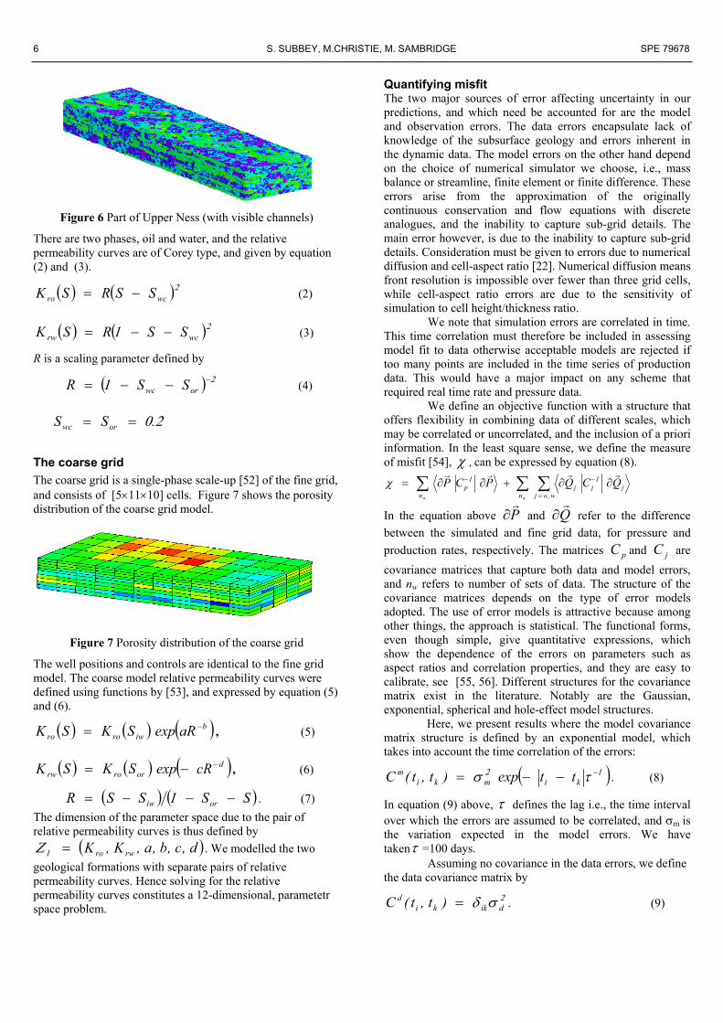
The fine grid The fine grid is the SPE 10th Comparison Solution Project model [51]. It is a geostatistical model defined on a three dimensional domain, being [1200x2200x170] cubic feet, and discretized into [60×220×85] cells. The top 70ft represents the Tarbert formation, and is a representation of a prograding near shore environment. The bottom 100ft is the Upper Ness, which consists of a part of the Brent sequence. Figure 5 and Figure 6 show the porosity distribution of the entire model, and part of the Upper Ness (with clearly visible channels), respectively. There are 4 producer wells in the corners of the model at constant 4000psi BHP, and a central water injector at constant injection rate of 5000bbl/day. All wells are vertical, and completed throughout the formation.

Figure 5 Porosity distribution of fine grid

6 S. SUBBEY, M.CHRISTIE, M. SAMBRIDGE SPE 79678

Quantifying misfit

The two major sources of error affecting uncertainty in our predictions, and which need be accounted for are the model and observation errors. The data errors encapsulate lack of knowledge of the subsurface geology and errors inherent in the dynamic data. The model errors on the other hand depend on the choice of numerical simulator we choose, i.e., mass balance or streamline, finite element or finite difference. These errors arise from the approximation of the originally continuous conservation and flow equations with discrete analogues, and the inability to capture sub-grid details. The main error however, is due to the inability to capture sub-grid details. Consideration must be given to errors due to numerical diffusion and cell-aspect ratio [22]. Numerical diffusion means front resolution is impossible over fewer than three grid cells, while cell-aspect ratio errors are due to the sensitivity of simulation to cell height/thickness ratio.

Figure 6 Part of Upper Ness (with visible channels)

There are two phases, oil and water, and the relative permeability curves are of Corey type, and given by equation (2) and (3).

( ) ( )2wcro SSRSK −= (2)

( ) ( )21 wcrw SSRSK −−= (3) We note that simulation errors are correlated in time.

This time correlation must therefore be included in assessing model fit to data otherwise acceptable models are rejected if too many points are included in the time series of production data. This would have a major impact on any scheme that required real time rate and pressure data.

R is a scaling parameter defined by

(4) ( 21 −−−= orwc SSR )

20.SS orwc == We define an objective function with a structure that

offers flexibility in combining data of different scales, which may be correlated or uncorrelated, and the inclusion of a priori information. In the least square sense, we define the measure of misfit [54], χ , can be expressed by equation (8). The coarse grid

jjn w,oj

jpn

QCQPCPww

∂∂+∂∂= −

=

− ∑ ∑∑ 11χ The coarse grid is a single-phase scale-up [52] of the fine grid, and consists of [5×11×10] cells. Figure 7 shows the porosity distribution of the coarse grid model. In the equation above and P∂ Q∂ refer to the difference

between the simulated and fine grid data, for pressure and production rates, respectively. The matrices C and are covariance matrices that capture both data and model errors, and n

p jC

w refers to number of sets of data. The structure of the covariance matrices depends on the type of error models adopted. The use of error models is attractive because among other things, the approach is statistical. The functional forms, even though simple, give quantitative expressions, which show the dependence of the errors on parameters such as aspect ratios and correlation properties, and they are easy to calibrate, see [55, 56]. Different structures for the covariance matrix exist in the literature. Notably are the Gaussian, exponential, spherical and hole-effect model structures.

Figure 7 Porosity distribution of the coarse grid

The well positions and controls are identical to the fine grid model. The coarse model relative permeability curves were defined using functions by [53], and expressed by equation (5) and (6).

( ) ( ) ( )biwroro aRexpSKSK −= , (5)

( ) ( ) ( )dorrorw cRexpSKSK −−= , (6)

( ) ( )SSSSR oriw −−−= 1 . (7)

Here, we present results where the model covariance matrix structure is defined by an exponential model, which takes into account the time correlation of the errors:

( )12 τσ −−−= kimkim ttexp)t,t(C . (8)

In equation (9) above, τ defines the lag i.e., the time interval over which the errors are assumed to be correlated, and σm is the variation expected in the model errors. We have takenτ =100 days.

The dimension of the parameter space due to the pair of relative permeability curves is thus defined by

. We modelled the two geological formations with separate pairs of relative permeability curves. Hence solving for the relative permeability curves constitutes a 12-dimensional, parametetr space problem.

( d,c,b,a,K,K rwro=1Ζ )Assuming no covariance in the data errors, we define

the data covariance matrix by 2σδ dikki

d )t,t(C = . (9)

SPE 79678 A STRATEGY FOR RAPID QUANTIFICATION OF UNCERTAINTY IN RESERVOIR PERFORMANCE PREDICTION 7

To illustrate, Figure 8 below gives an example of the covariance structures for the oil rate. Given a point m in model space, the likelihood that the observation O can be obtained by is given by m

( ) ( 2χ−exp~mOp ). (10)

The refinement criterion for the Neighbourhood Approximation algorithm is based on the rank of the misfit . This is defined as

( )( ) 2χ=−= mOplog . (11)

a. Data errors b. Model errors

Figure 8 Covariance structures

Results and discussion We used the NA-algorithm to generate 312 models using ECLISPE, sampling a 12-dimensional space.

We first investigate our ability to match the history data, and quantify the uncertainty during the history matching period. Figure 9 shows the match of the oil rate uncertainty curves to the observed (noisy) data. The plot also shows the P10 — P90 profiles, and our method for calculating these, is described below. The P10 — P90 profiles define the uncertainty envelope, and include most of the field data. The inability of the uncertainty envelope to encapsulate the observed data for time less than 100 days is largely due to our assumption of zero model and data errors, for time equals zero. Figure 10 shows plots of the 1-dimensional probability plots for the first four of the model parameters, using ECLIPSE, while Figure 11 shows equivalent plots using 3DSL. The 1-dimensional probability plots are computed using MCMC on the response surface, and represent single parameter effects, averaged over all the other parameters. Calculating the 1D-marginals in practice requires the computation of a generic Bayesian integral J, expressed as

( ) ( )dmmpmgJ ∫= . (12)

Here represents the distribution of an attribute of interest, e.g., a distribution of the model parameters, and is the posterior probability distribution. A Monte Carlo presentation of equation (12) is given by equation (13), where N is the number of models in the ensemble used in the

evaluation, and

( )mg

( )mp

( )mh is the sampling density.

( k

hmg

∑=

mn

kf1

Qwk

k∑

wk

k∑

) ( )( )∑

=

=N

k k

k

mmp

NJ

1

1 (13)

The MCMC approach is to sample the misfit surface, and generate a completely new ensemble of models. The value of J is then calculated using the newly generated ensemble, rather than the original models. The aim is to perform the sampling in such as way that the sampling density of the new ensemble approximates the posterior probability distribution ( )mp . In that case, the generic integral reduces to an average of the distribution of the resampled models. The 3DSL results were obtained using 984 history match models. Whereas some of the parameters (e.g., parameter 2 and 3) appear to have similar shapes, others differ considerably. The differences are likely to be due to the different errors in each simulator. If we computed detailed error models for each of the simulators and incorporated this into our misfit calculations, it is likely that the differences between the 1-dimensional plots would be significantly less.

The next stage in our uncertainty quantification process is to assess our ability to forecast future fine grid performance, and to quantify the uncertainty in the forecast. As an initial step, we have assessed the ability of the maximum likelihood model in predicting the fine grid behaviour. Figure 12 shows plots of the maximum likelihood prediction for the oil and water rates, and the field average pressure. We observe that for this particular case, the maximum likelihood model is highly accurate in predicting the fine grid response. Our emphasis however, is not on the performance of a single best model, i.e., the maximum likelihood model, but on the generation of an uncertainty envelope, using the complete ensemble of models generated.

To quantify the uncertainty in our predictions, we run a long chain of the MCMC algorithm on the misfit surface and performed a Bayes update of the probabilities. We monitored the frequency of visits to each Voronoi cell during the random walk. Thus we are able to calculate the relative probability wj of each model mj in the ensemble of size nm, based on the frequency fj, using equation (15). Since the MCMC algorithm samples from the posterior distribution, the calculated probability is representative of the posterior probability of each model.

=k

jj fw . (14)

Assuming Gaussian statistics, we calculate the mean and standard deviation (first and second moments) of the pressure and production profiles by

( ) ( )ttQ k=1

, (15)

( ) ( ) ( ) 2

12

2tQtQtQ k −= . (16)

Using these parameters, we determined P10 and P90 cut-off for each of the predicted profiles. We note that during the MCMC walk, new models are generated, which were not in the

8 S. SUBBEY, M.CHRISTIE, M. SAMBRIDGE SPE 79678

original ensemble. Figure 13 shows the uncertainty envelope generated

for oil, water and the average pressure. The plot shows the P10 and P90 profiles as well as the mean and maximum likelihood results. We observe that the P10 — P90 profiles envelope the maximum likelihood prediction as well as the fine grid data. Figure 14 shows a plot of the fractional uncertainty in the prediction, for the oil rate. The profile of this curve shows the effect of the uncertainties up to 300 days.

As mentioned previously, the results presented in this paper are based on using 312 models for ECLIPSE, and 984 models for 3DSL. Generating either of these model ensembles required an average of 3 hours on a single CPU machine. Realistic uncertainty quantification however, requires performing several thousands of forward modelling. Running thousands of forward modelling on a single CPU machine, even for very simple models, is a daunting task. We have therefore investigated the use of parallel computing in generating multiple history match models. Our approach involves running a parallel version of the NA-algorithm on multiple CPUs. This paper presents some of our results.

Figure 15 shows results from our speedup tests. This graph was created by sampling for a total of 500 models using the parallel version of the NA-algorithm. The graph shows the total run-time as a function of the number of CPUs. The graph shows that generating 500 models takes less than 8.5 minutes on 36 CPUs, compared with 3 hours on the single CPU machine.

In our particular case, we have access to 64 CPUs. Using the speed-up results, we can extrapolate to expect a speed-up of approximately 43 for the total of 64 CPUs. This gives an approximate 430 CPU hours for 10 hours. We can expect to generate at least 10,000 history match models overnight.

Conclusions We have showed the use of the Neighbourhood Approximation algorithm in generating multiple history match models. The approach presented is able to incorporate both data and model errors in quantifying the degree of model fit to the observed data, and in defining the model likelihood.

Using the complete ensemble of models generated and a MCMC approach, we have used the Neighbourhood Approximation algorithm in a Bayesian framework, in quantifying uncertainty in prediction of the fine grid profiles.

To demonstrate the strength of the algorithm in generating history match models, and in quantifying uncertainty, we have used a benchmark data set (SPE 10th Comparison Solution Project) for which the true solution is known. Our results show that in this case the maximum likelihood model is a good forward predictor, and that the true solution lies within the uncertainty envelop predicted by the algorithm.

This paper has demonstrated two distinct approaches for achieving speed-up in generating multiple history matching models. In the first approach, we have presented results using a parallel version of the Neighbourhood approximation algorithm on a Linux cluster using the MPI standard. Our result shows that it is practical to generate over

10,000 history match models overnight. We have also highlighted the use of streamline

simulation to achieve speed-up in exploring parameter space and rapidly identify regions of parameter space for further exploration using a finite difference simulator. Our results show that the 1-dimensional probability distribution of the model parameters is dependent on quantifying the model and data errors.

Acknowledgement The authors wish to thank the sponsors of the Heriot-Watt University Uncertainty Project for permission to publish these results. Furthermore we thank GeoQuest for the use of ECLIPSE, Streamsim Technologies, for the use of 3DSL, and the UK Engineering and Physical Sciences Research Council for a JREI Grent to purchase the Beowulf Cluster.

SPE 79678 A STRATEGY FOR RAPID QUANTIFICATION OF UNCERTAINTY IN RESERVOIR PERFORMANCE PREDICTION 9

References 1. Hadamard, J., Lectures on the Cauchy Problem in Linear

Partial Differential Equations, Yale University Press, 1923.

2. Bissell, R. C., Killough, J., and Sharma, Y., “Reservoir History Matching Using the Method of Gradients”, SPE 24265, 1992.

3. Lépine, O. J., et al., “Uncertainty Analysis in Predictive Reservoir Simulation Using Gradient Information’, SPEJ, Vol.4, Nr. 3, 1999.

4. Phan V., and Horne, R. N., “Determining Depth-Dependent Reservoir Properties Using Integrated Data Analysis”, SPE 56423, 1999.

5. Roggero, F., “Direct Selection of Stochastic Model Realizations Constrained to Hsitory Data”, SPE 38731, 1997.

6. Portella, R. C. M., and Prais, F. “Use of Automatic History Matching and Geostatistical Simulation to Improve Production Forecast”, SPE 53976, 1999.

7. Romero, C. E., Carter, J. N., Zimmerman, R. W. and Gringarten, A. C., “Improved reservoir characterization through evolutionary computation”, SPE 62942, 2000.

8. Schulze-Riegert, R. W., Axmann, J. K., Haase, O., Rian, D. T. and You, Y.-L., “Optimization methods for history matching of complex reservoirs”, SPE 66393, 2001.

9. Chen, W. H., Gavalas, G. R., Seinfeld, J. H., and Wasserman, M. L., “A New Algorithm for Automatic History Matching”, SPE 4545, 1973.

10. Gill, P. E., Murray, W., and Wright, M. H., Practical Optimization, Academic Press, New York, 1981.

11. McCormick, G. P., and Ritter, K., “Methods of Conjugate Directions versus Quasi-Newton Methods”, Math. Programming 3, pp 101-111, 1972.

12. Shanno, D. F., “Conjugate Gradient Methods with Inexact Searches”, Math of Oper. Res. 3, pp. 244-256, 1978.

13. Yang, P. H., and Watson, A. T., “Automatic History Matching with Variable-Metric Method”, SPE 16977, 1987.

14. Zhang, J., Dupuy, A., and Bissell, R. C., “Use of Optimal Control Theory for History Matching”, 2nd International Conference on Inverse Problems: Theory and Practice, France, June 9-14, 1996.

15. Haldorsen, H. H., and Damsleth, E., “Stochastic Modelling”, JPT, pp 404-412, April 1990.

16. Ouenes, A., Bhagavan, S., Bunge, P. H., and Travis, B. J., “Application of Simulated Annealing and Other Global Optimization Methods to Reservoir Description: Myths and Realities”, SPE 28415, 1994.

17. Sen, M. K., Gupta, A. D., Stoffa, P. L., Lake, L. W., and Pope, G. A., “Stochastic Reservoir Modeling Using Simulated Annealing and Genetic Algorithm”, SPE 24754, 1992.

18. Holland, J. H., “Genetic Algorithms”, Scientific

American, pp. 66-72, July 1992. 19. Sambridge, M., “Geophysical inversion with a

Neighbourhood Algorithm, Part 1: Searching a parameter space”, (Geophysical Journal International, 1999a).

20. Kirkpatrick, S., Gelatt, Jr., C. D., and Vecchi, M. P., “Optimization by Simulated Annealing”, Science, Vol. 220, No. 4598, 13 May 1983.

21. Okabe, A., Boots, B., and Sugihara, K., Spatial Tessellations Concepts and Applications of Voronoi diagrams, John-Wiley & Sons, England, 1992.

22. Christie, M., MacBeth, C., and Subbey, S., “Multiple history-match models for Teal South”, The Leading Edge, 2002.

23. Subbey, S., Christie, M., and Sambridge, M., “Uncertainty Reduction in Reservoir Modeling”, Con. Maths., Vol. 295, pp. 457-467, 2002.

24. Geman, S., and Geman, D., “Stochastic Relaxation, Gibbs Distribution and the Bayesian Restoration of Images”, IEEE Trans. Patt. Analysis Mach. Int. (6): 721-741, 1984.

25. Cheshire, I. M., and Bowen, G., “Parallelization in Reservoir Simulation”, SPE 23657, 1992.

26. Zhiyuan, M, Fengjiang, J., Xiangming, X., and Jiachang, S., “Simulation of Black Oil Reservoir on Distributed Memory Parallel Computers and Workstation Clusters”, SPE 29937, 1995.

27. Leitao, H. C., and Schiozer, D. , “A New Automated History Matching Algorithm Improved by Parallel Computing”, SPE 53977, 1999.

28. Schiozer, D. J., “Use of Reservoir Simulation. Parallel Computing and Optimization Techniques to Accelerate History Matching and Reservoir Management Decisions”, SPE 53979, 1999.

29. Schiozer, D. J. and Sousa, S. H. G., “Use of External Parallelization to Improve History Matching”, SPE 39062, 1997.

30. Ouenes, A., Weiss, W., Sultan, A. J., Nati, A. D., and Anwar, J., “Parallel Reservoir Automatic History Matching Using a Network of Workstations and PVM”, SPE 29107, 1995.

31. Ouenes, A., and Saad, N, “A New, Fast Parallel Simulated Annealing Algorithm for Reservoir Characterization”, SPE 26419, 1993.

32. LeVeque, R. J., Numerical Methods for Conservative Laws, Birkhauser-Verlag, Bassel, 1990.

33. Lolomari, T., Bratvedt, K., Crane, M., Millihen, W. J., Tyrie, J. J., “The Use of Streamline Simulation in Reservoir Management: Methodology and Case Studies”, SPE 63157, 2000.

34. Thiele, M. R., Batycky, R. P., Blunt, M. J., “A Streamline-Based 3D Field-Scale Compositional Reservoir Simulator”, SPE 38889, 1997.

35. Emanuel, A. S., Milliken, W. J., “History Matching Finite Difference Models with 3D Streamlines”, SPE 49000, 1998.

36. Hastings, J. J., Muggeridge, A. H., and Blunt, M. J., “A New Streamline Method for Evaluating Uncertainty in Small-Scale, Two-Phase Flow Properties”, SPE 66349,

10 S. SUBBEY, M.CHRISTIE, M. SAMBRIDGE SPE 79678

2001. 37. Sivia, D. S., Data Analysis – A Bayesian Tutorial,

Claredon Press, Oxford, 1996. 38. Hansen, K. M., Cunningham, G. S., and McKee, R. J.,

“Uncertainty Assessment for Reconstructions Based on Deformable Geometry”, Int. J. Imaging Syst. Technology, Vol. 8, 506-512, 1997.

39. Cunha, L. B., Oliver, D. S., Rednar, R. A., and Reynolds, A. C., “A Hybrid Markov Chain Monte Carlo Method for Generating Permeability Fields Conditioned to Multiwell Pressure Data and Prior Information”, SPEJ 3 (3): 261− 271, 1998.

40. Oliver, D. S., Cunha, L. B. and Reynolds, A. C., “Markov chain Monte Carlo methods for conditioning a permeability field to pressure data”, Mathematical Geology, Vol. 29, Nr. 1, 61-91, 1997.

41. Omre, H., Tjelmeland, H., and Wist, H. T., “Uncertainty in History Matching − Model Specification and Sampling Algorithms”, Tech. Rep. Stats. No 6/1999, Dept. of Mathematical Sciences, NTNU, Norway, 1999.

42. Barker, J. W., and Cuypers M., “Quantifying Uncertainty in Production Forecasts: Another Look at the PUNQ-S3 Problem”, SPE 62925, 2000.

43. Floris, F. J. T., Bush, M. D., Cuypers, M., Roggero, F., and Syversveen, A.-R., “Comparison of Production Forecast Uncertainty Quantification Methods−An Integrated Study”, Paper resented at 1st Conference on Petroleum Geostatistics, Toulouse, France, 1999

44. Oliver, D. S., “Incorporation of Transient Pressure Data into Reservoir Characterization”, In Situ 18(3):243-275, 1994.

45. Chu, L., Reynolds, A. C., and Oliver, D. S., “Computation of Sensitivity Coefficients for Conditioning the Permeability Field to Well-Test Data”, In Situ 19(2): 179-223, 1995.

46. Kitanidis, P. K., “Quasi-Linear Geostatistical Theory for Inversing”, Water Resour. Res. 31(10): 2411-2419, 1995.

47. Oliver, D. S., He, N., and Reynolds, A. C., “Conditioning Permeability Fields to Pressure Data”, In ECMOR V, pp. 1-11, 1996.

48. Bissell, R. C., Dubrule, O., Lamy, P., Swaby, P., and Lépine, O., “Combining Geostatistical Modelling with Gradient Information for History Matching: The Pilot Method”, SPE 38730, 1997.

49. Liu, N., Betancourt, S., and Oliver, D. S., “Assessment of Uncertainty Assessment Methods”, SPE 71624, 2001.

50. Sambridge, M., “Geophysical inversion with a Neighbourhood Algorithm, Part 2: Appraising the ensemble”, (Geophysical Journal International, 1999b).

51. Christie, M. A., and Blunt, M. J., “Tenth SPE Comparative Solution Project: A Comparison of Upscaling Techniques”, SPE 66599, 2000.

52. Christie, M. A., “Upscaling for Reservoir Simulation”, JPT, SPE 37324, 1996.

53. Chierici, G., “Novel Relations for Drainage and Imbibition Relative Permeabilities”, SPE 10165, 1981.

54. Tarantola, A., Inverse Problem Theory, Methods for Data

Fitting and Model Parameter Estimation, Elsevier Science Publishers, Amsterdam, 1987.

55. Glimm, J., Hou, S., Kim, H., and Sharp, D. H., “A Probability Model for Errors in the Numerical Solutions of a Partial Differential Equation”. Computational Fluid Dynamics Journal, Vol. 9, 485-493, 2001.

56. Glimm, J., Hou, S., Lee, Y., and Sharp, D. H., “Prediction of Oil Production with Confidence Intervals”, SPE 66350, 2001.

LIST OF FIGURES

2000

3000

4000

5000

6000

7000

8000

0 100 200 300time (days)

Max likelihood

Mean

P10

P90

Field

Figure 9 Match to noisy data (oil rate)

SPE 79678 A STRATEGY FOR RAPID QUANTIFICATION OF UNCERTAINTY IN RESERVOIR PERFORMANCE PREDICTION 11

0

0.05

0.1

0.15

0.2

0.25

0.3

0.35

0 3 6 9 1 value (parameter 1)

0

0.05

0.1

0.15

0.2

0.25

0.3

0 1 2 3 4 value (param eter 3)

0

0.05

0.1

0.15

0.2

0.25

0 0.5 1 1.5 2 2.5 3 3.5 4 value (parameter 2)

0

0.04

0.08

0.12

0.16

0.2

0 0.5 1 1.5 2

20

0 .1

0 .2

0 .3

0 .4

0 2 4 6 8 1 0 1v a lu e s ( p a r a m e te r 1 )

0

0 .0 4

0 .0 8

0 .1 2

0 .1 6

0 1 2 3 4 v a lu e (p a ra m e te r 3 )

0

0 .0 5

0 .1

0 .1 5

0 0 .5 1 1 .5 2

0

0 .0 5

0 .1

0 .1 5

0 .2

0 .2 5

0 1 2 3 4 v a lu e (p a ra m e te r 2 )

2

Figure 10 1D marginals (ECLIPSE)

Figure 11 1D marginals (3DSL) va lue (param eter 4) v a lu e (p a ra m e te r 4 )

12 S. SUBBEY, M.CHRISTIE, M. SAMBRIDGE SPE 79678

Figure 13 Uncertainty quantification Figure 12 Maximum likelihood model performance

0.

Figure 14 Fractional uncertainty (oil rate) Figure 15 Results from parallel computing

4000

5000

6000

0 500 1000 1500 2000time (days)

Fine grid Maximum likelihood model

Mean P10 P90

a. Oil rate

b. Water rate

c. Average pressure

a. Oil rate uncertainty

b. Water rate uncertainty

c. Average pressure uncertainty

0

2000

4000

6000

8000

0 500 1000 1500 2000 time (days)

Fine grid

Maximum likelihood model

History match time

0

1000

2000

3000

4000

5000

0 500 1000 1500 2000 time (days)

Fine grid

Maximum likelihood model

History match time

0

1500

3000

4500

6000

0 500 1000 1500 2000 time (days)

Fine grid

Maximum likelihood model

History match time

0

2000

4000

6000

8000

0 500 1000 1500 2000 time (days)

Fine grid

Maximum likelihood model

Mean

P10

P90

0

1000

2000

3000

4000

5000

0 500 1000 1500 2000 time (days)

Fine grid

Maximum likelihood model

Mean

P10

P90

0.0

0.1

0.2

3

0.0 500.0 1000.0 1500.0 2000.0time (days)

0

0.5

1

1.5

2

2.5

3

3.5

0 6 12 18 24 30 36number of CPUs

time

(hou

rs)