Embed Size (px)
Citation preview
SPE 166098
Managing Shut-in Time to Enhance Gas Flow Rate in Hydraulic Fractured Shale Reservoirs: a Simulation Study Perapon Fakcharoenphol, SPE; Mehmet Torcuk, SPE, Colorado School of Mines, Antoine Bertoncello, SPE, Hess Corporation; Hossein Kazemi, SPE; Yu-Shu Wu, SPE, Colorado School of Mines; Jon Wallace, SPE; and Matt Honarpour, SPE, Hess Corporation
Copyright 2013, Society of Petroleum Engineers This paper was prepared for presentation at the SPE Annual Technical Conference and Exhibition held in New Orleans, Louisiana, USA, 30 September–2 October 2013. This paper was selected for presentation by an SPE program committee following review of information contained in an abstract submitted by the author(s). Contents of the paper have not been reviewed by the Society of Petroleum Engineers and are subject to correction by the author(s). The material does not necessarily reflect any position of the Society of Petroleum Engineers, its officers, or members. Electronic reproduction, distribution, or storage of any part of this paper without the written consent of the Society of Petroleum Engineers is prohibited. Permission to reproduce in print is restricted to an abstract of not more than 300 words; illustrations may not be copied. The abstract must contain conspicuous acknowledgment of SPE copyright.
Abstract Some shale gas and oil wells undergo month-long shut-in times after multi-stage hydraulic fracturing well stimulation. Field data indicate that in some wells, such shut-in episodes surprisingly increase the gas and oil flow rate. In this paper, we report a numerical simulation study that supports such observations and provides a potentially viable underlying imbibition and drainage mechanism. In the simulation, the shale reservoir is represented by a triple-porosity fracture-matrix model, where the fracture forms a continuum of interconnected network created during the well simulation while the organic and non-organic matrices are embedded in the fracture continuum. The effect of matrix wettability, capillary pressure, relative permeability, and osmotic pressure, that is, chemical potential characteristics are included in the model.
The simulation results indicate that the early lower flow rates are the result of obstructed fracture network due to high water saturation. This means that the injected fracturing fluid fills such fractures and blocks early gas or oil flow. Allowing time for the gravity drainage and imbibition of injected fluid in the fracture-matrix network is the key to improving the hydrocarbon flow rate during the shut-in period.
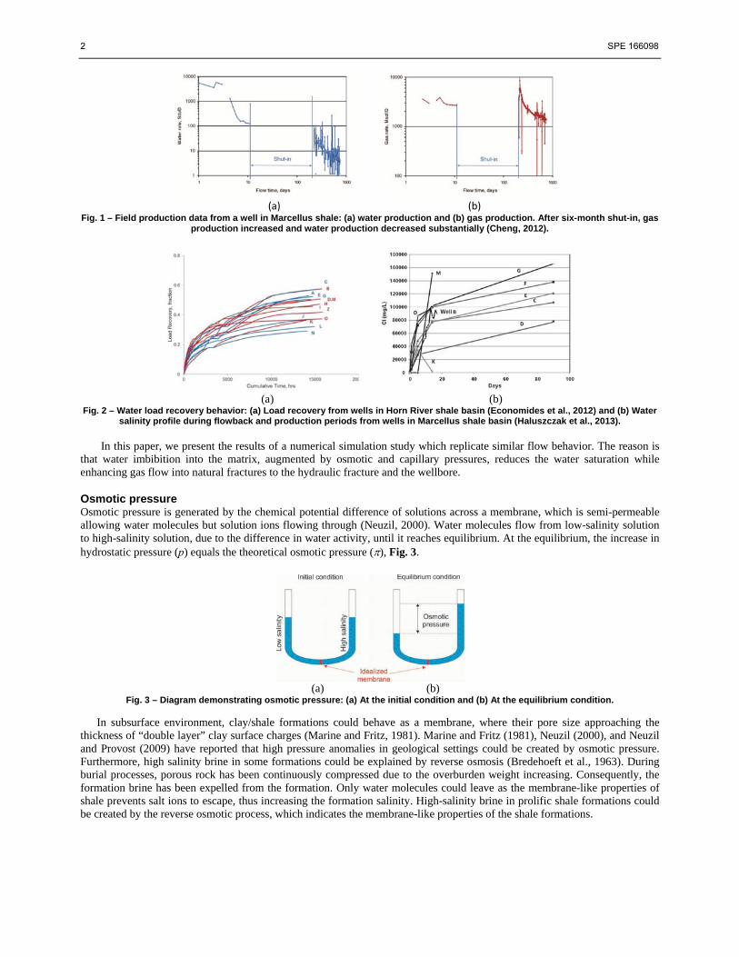
Introduction Some shale gas and oil wells undergo month-long shut-in times after multi-stage hydraulic fracture stimulation. Field data indicate that in some wells, such shut-in episodes surprisingly increase the gas and oil flow rate. For example, Fig. 1 shows the effect of an extended shut-in on production of a multi-stage hydraulically fractured well in Marcellus shale (Cheng, 2012). The well was flowed back, after hydraulic fracture stimulation, for a short period before it underwent a six-month shut-in period. When the well was reopened after six months of shut in, gas production rate increased and water production rate decreased significantly. The question is what caused this apparent anomaly?
Water load recovery and flowback behavior Field experience indicates that water load recovery could be as low as 5% of the total injection volume in Haynesville shale to as high as 50% of that in Barnett and Marcellus shales (King, 2012). Number of mechanisms could contribute to the low-recovery, including extra-trapped water due to changing in natural fractures width that increasing during injection and decreasing during production periods (Economides et al., 2012), water imbibition into shale matrix by capillary pressure (Cheng, 2012).
Flow back water analyzed by Haluszczak et al. (2013) indicates that formation brine in shale basin could be higher than 150,000 ppm, Fig. 2b. As the typical fracturing fluid comprises low-salinity water, in many cases it is in the range of 1,000 ppm, significant salinity contrast would be expected. This major salinity difference could lead to substantial chemical potential differences creating large osmotic pressure and driving filtrate from natural fractures into shale matrix block.
2 SPE 166098
(a) (b) Fig. 1 – Field production data from a well in Marcellus shale: (a) water production and (b) gas production. After six-month shut-in, gas
production increased and water production decreased substantially (Cheng, 2012).
(a) (b)
Fig. 2 – Water load recovery behavior: (a) Load recovery from wells in Horn River shale basin (Economides et al., 2012) and (b) Water salinity profile during flowback and production periods from wells in Marcellus shale basin (Haluszczak et al., 2013).
In this paper, we present the results of a numerical simulation study which replicate similar flow behavior. The reason is
that water imbibition into the matrix, augmented by osmotic and capillary pressures, reduces the water saturation while enhancing gas flow into natural fractures to the hydraulic fracture and the wellbore.
Osmotic pressure Osmotic pressure is generated by the chemical potential difference of solutions across a membrane, which is semi-permeable allowing water molecules but solution ions flowing through (Neuzil, 2000). Water molecules flow from low-salinity solution to high-salinity solution, due to the difference in water activity, until it reaches equilibrium. At the equilibrium, the increase in hydrostatic pressure (p) equals the theoretical osmotic pressure (), Fig. 3.
(a) (b)
Fig. 3 – Diagram demonstrating osmotic pressure: (a) At the initial condition and (b) At the equilibrium condition.
In subsurface environment, clay/shale formations could behave as a membrane, where their pore size approaching the thickness of “double layer” clay surface charges (Marine and Fritz, 1981). Marine and Fritz (1981), Neuzil (2000), and Neuzil and Provost (2009) have reported that high pressure anomalies in geological settings could be created by osmotic pressure. Furthermore, high salinity brine in some formations could be explained by reverse osmosis (Bredehoeft et al., 1963). During burial processes, porous rock has been continuously compressed due to the overburden weight increasing. Consequently, the formation brine has been expelled from the formation. Only water molecules could leave as the membrane-like properties of shale prevents salt ions to escape, thus increasing the formation salinity. High-salinity brine in prolific shale formations could be created by the reverse osmotic process, which indicates the membrane-like properties of the shale formations.
SPE 166098 3
Osmotic pressure () is described by (Marine and Fritz, 1981):
14.5 ln I
II
RT a
V a (1)
where,
Ia , IIa water activity of system I and II; low-salinity I and high-salinity II, Water activity for fresh water is 1.0.
R gas constant, equal to 0.082 atm. (kg-mol.K)-1 T temperature, °K
V partial molar volume, l/kg-mol
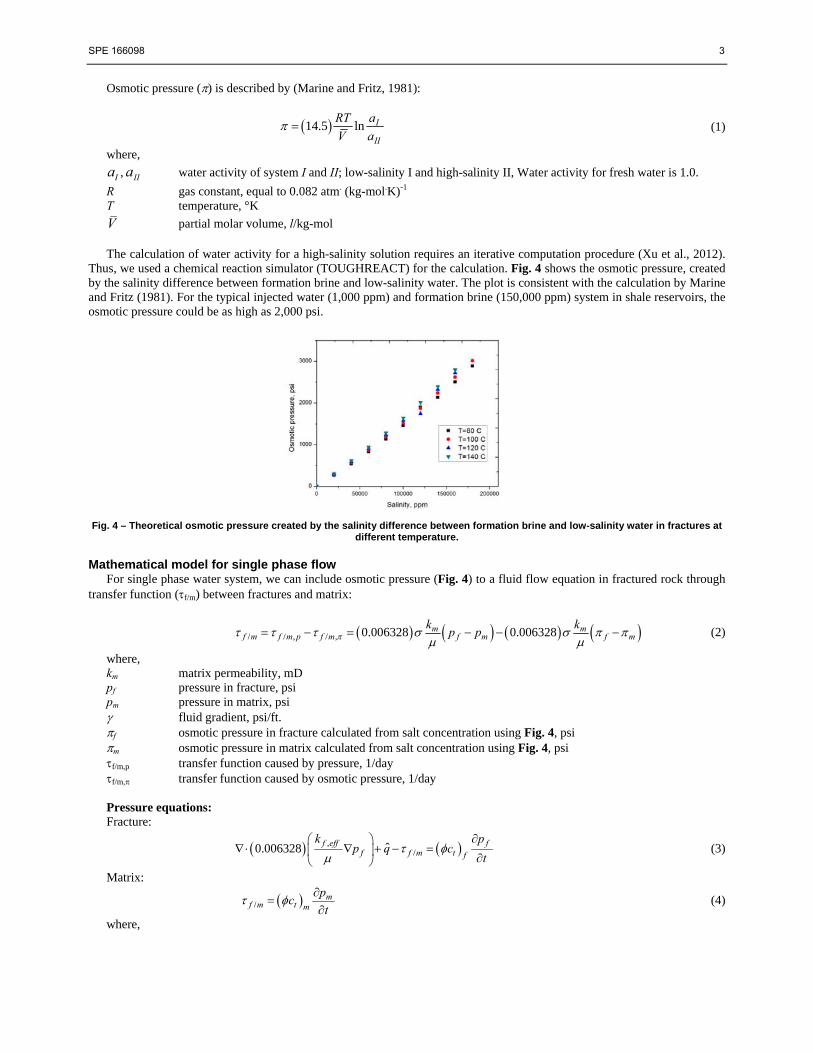
The calculation of water activity for a high-salinity solution requires an iterative computation procedure (Xu et al., 2012). Thus, we used a chemical reaction simulator (TOUGHREACT) for the calculation. Fig. 4 shows the osmotic pressure, created by the salinity difference between formation brine and low-salinity water. The plot is consistent with the calculation by Marine and Fritz (1981). For the typical injected water (1,000 ppm) and formation brine (150,000 ppm) system in shale reservoirs, the osmotic pressure could be as high as 2,000 psi.
Fig. 4 – Theoretical osmotic pressure created by the salinity difference between formation brine and low-salinity water in fractures at
different temperature. Mathematical model for single phase flow
For single phase water system, we can include osmotic pressure (Fig. 4) to a fluid flow equation in fractured rock through transfer function (f/m) between fractures and matrix:
/ / , / , 0.006328 0.006328m mf m f m p f m f m f m
k kp p
(2)
where, km matrix permeability, mD pf pressure in fracture, psi pm pressure in matrix, psi fluid gradient, psi/ft.f osmotic pressure in fracture calculated from salt concentration using Fig. 4, psi m osmotic pressure in matrix calculated from salt concentration using Fig. 4, psi f/m,p transfer function caused by pressure, 1/day f/m, transfer function caused by osmotic pressure, 1/day Pressure equations: Fracture:
,/ˆ0.006328 f eff f
f f m t f
k pp q c
t
(3)
Matrix:
/m
f m t m
pc
t
(4)
where,
4 SPE 166098
ct total compressibility, 1/psikf,eff effective fracture permeability, md q̂ sink/source term, 1/day
t time, day porosity, fraction fluid viscosity, cp Salt concentration equations: In this paper we assumed that salt is not absorbed on the surface of rock grain. In fracture:
,/ , / ,
/ , / , /
ˆ0.006328 f efff f f f m p f m p
f ff m f m f m f m t ff
kC p C q C
p CC D C C C c
t t
(5)
In matrix:
// , / ,m m
f m f m t mf m p f m m
p CC C D C C C c
t t
(6)
where, Cf, Cm salt concentration in fracture and matrix, ppm Df/m diffusion coefficient between fracture and matrix, ft2/day To examine the mathematical model, we modeled and compared our simulation to the osmotic pressure measurement for
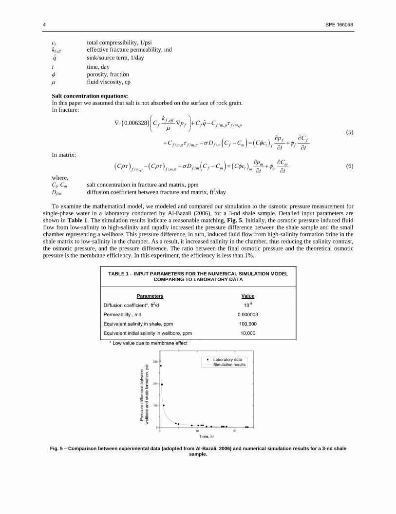
single-phase water in a laboratory conducted by Al-Bazali (2006), for a 3-nd shale sample. Detailed input parameters are shown in Table 1. The simulation results indicate a reasonable matching, Fig. 5. Initially, the osmotic pressure induced fluid flow from low-salinity to high-salinity and rapidly increased the pressure difference between the shale sample and the small chamber representing a wellbore. This pressure difference, in turn, induced fluid flow from high-salinity formation brine in the shale matrix to low-salinity in the chamber. As a result, it increased salinity in the chamber, thus reducing the salinity contrast, the osmotic pressure, and the pressure difference. The ratio between the final osmotic pressure and the theoretical osmotic pressure is the membrane efficiency. In this experiment, the efficiency is less than 1%.
TABLE 1 – INPUT PARAMETERS FOR THE NUMERICAL SIMULATION MODEL COMPARING TO LABORATORY DATA
Parameters
Value
Diffusion coefficient*, ft2/d
Permeability , md
10-8
0.000003
Equivalent salinity in shale, ppm 100,000
Equivalent initial salinity in wellbore, ppm 10,000
* Low value due to membrane effect
Fig. 5 – Comparison between experimental data (adopted from Al-Bazali, 2006) and numerical simulation results for a 3-nd shale sample.
SPE 166098 5
Neuzil and Provost (2009) have thoroughly reviewed public experimental data and reported consistently low membrane
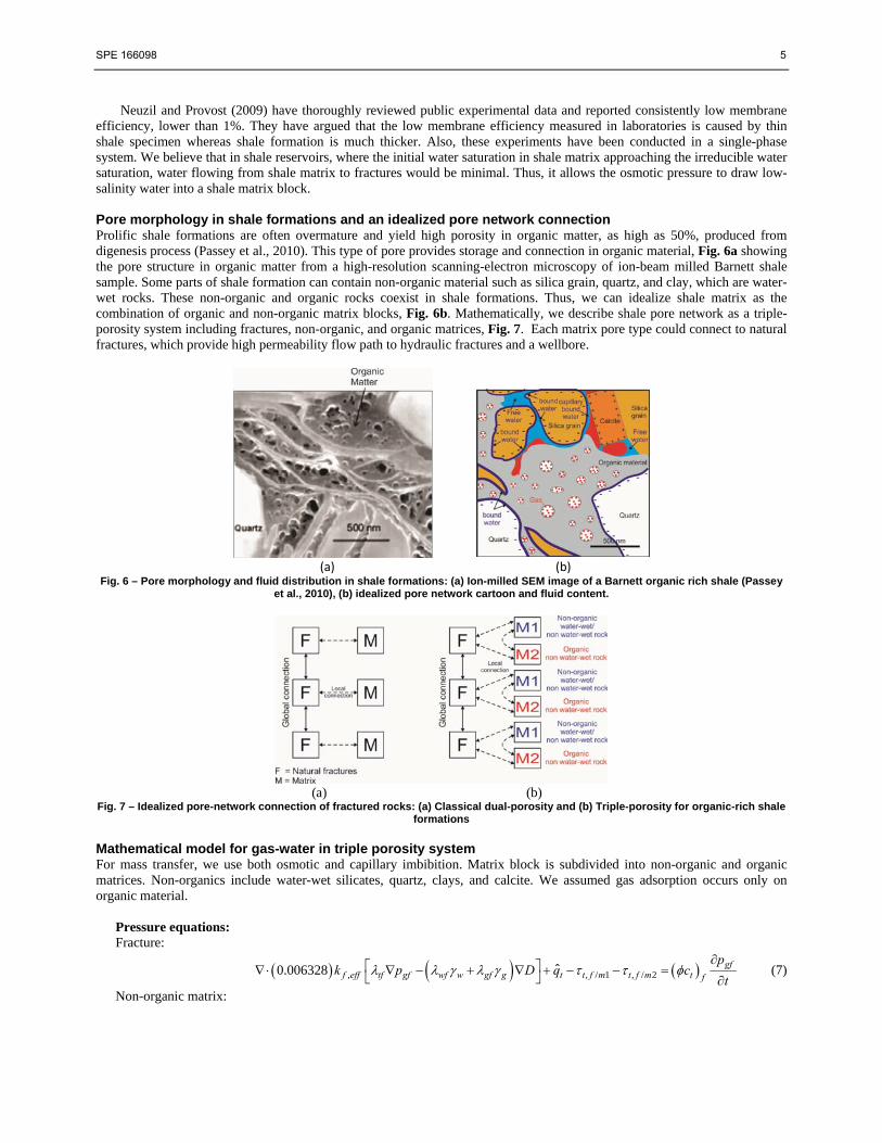
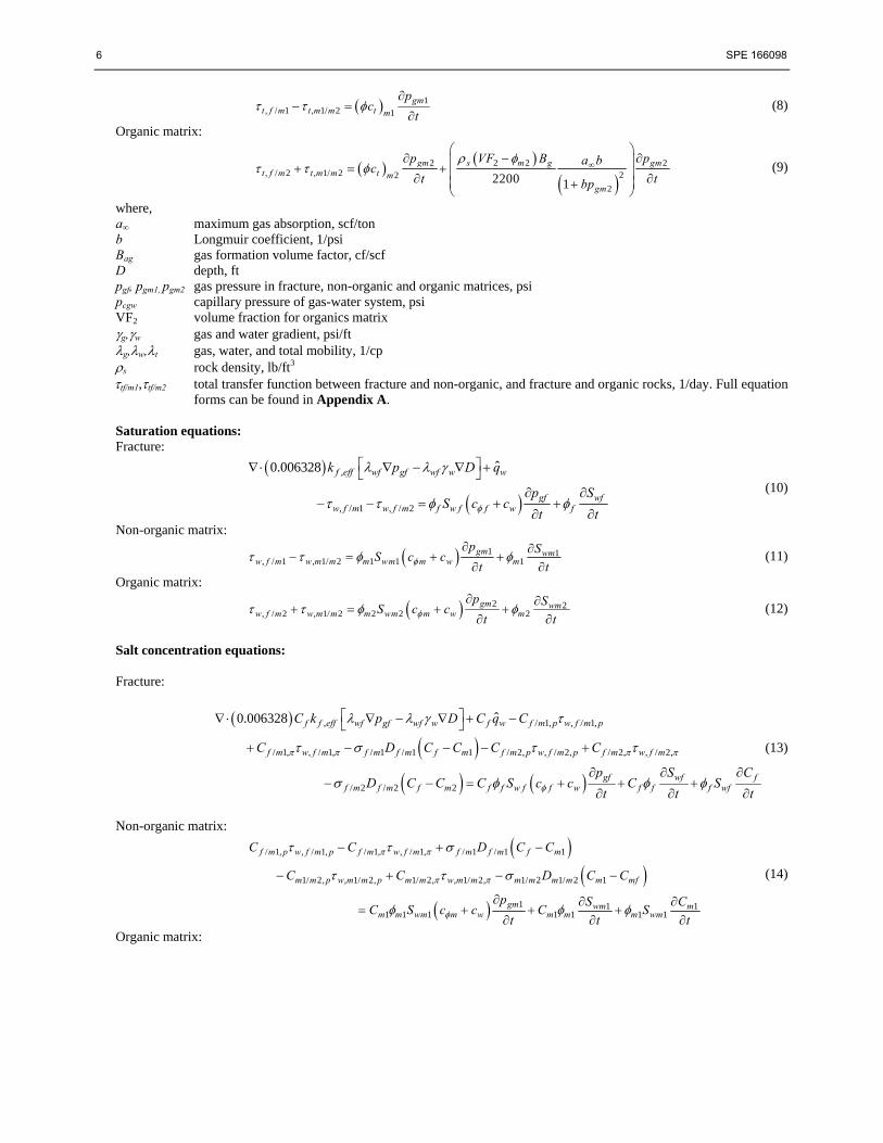
efficiency, lower than 1%. They have argued that the low membrane efficiency measured in laboratories is caused by thin shale specimen whereas shale formation is much thicker. Also, these experiments have been conducted in a single-phase system. We believe that in shale reservoirs, where the initial water saturation in shale matrix approaching the irreducible water saturation, water flowing from shale matrix to fractures would be minimal. Thus, it allows the osmotic pressure to draw low-salinity water into a shale matrix block. Pore morphology in shale formations and an idealized pore network connection Prolific shale formations are often overmature and yield high porosity in organic matter, as high as 50%, produced from digenesis process (Passey et al., 2010). This type of pore provides storage and connection in organic material, Fig. 6a showing the pore structure in organic matter from a high-resolution scanning-electron microscopy of ion-beam milled Barnett shale sample. Some parts of shale formation can contain non-organic material such as silica grain, quartz, and clay, which are water-wet rocks. These non-organic and organic rocks coexist in shale formations. Thus, we can idealize shale matrix as the combination of organic and non-organic matrix blocks, Fig. 6b. Mathematically, we describe shale pore network as a triple-porosity system including fractures, non-organic, and organic matrices, Fig. 7. Each matrix pore type could connect to natural fractures, which provide high permeability flow path to hydraulic fractures and a wellbore.
(a) (b) Fig. 6 – Pore morphology and fluid distribution in shale formations: (a) Ion-milled SEM image of a Barnett organic rich shale (Passey
et al., 2010), (b) idealized pore network cartoon and fluid content.
(a) (b)
Fig. 7 – Idealized pore-network connection of fractured rocks: (a) Classical dual-porosity and (b) Triple-porosity for organic-rich shale formations
Mathematical model for gas-water in triple porosity system For mass transfer, we use both osmotic and capillary imbibition. Matrix block is subdivided into non-organic and organic matrices. Non-organics include water-wet silicates, quartz, clays, and calcite. We assumed gas adsorption occurs only on organic material.
Pressure equations: Fracture:
, , / 1 , / 2ˆ0.006328 gff eff tf gf wf w gf g t t f m t f m t f
pk p D q c
t
(7)
Non-organic matrix:
6 SPE 166098
1, / 1 , 1/ 2 1
gmt f m t m m t m
pc
t
(8)
Organic matrix:
2 2 2 2
, / 2 , 1/ 2 22
22200 1
gm s m g gmt f m t m m t m
gm
p VF B pa bc
t tbp
(9)
where, a∞ maximum gas absorption, scf/ton b Longmuir coefficient, 1/psi Bag gas formation volume factor, cf/scf D depth, ft pgf, pgm1, pgm2 gas pressure in fracture, non-organic and organic matrices, psi pcgw capillary pressure of gas-water system, psi VF2 volume fraction for organics matrix g,w gas and water gradient, psi/ft g,w,t gas, water, and total mobility, 1/cp s rock density, lb/ft3 tf/m1,tf/m2 total transfer function between fracture and non-organic, and fracture and organic rocks, 1/day. Full equation
forms can be found in Appendix A. Saturation equations: Fracture:
,
, / 1 , / 2
ˆ0.006328 f eff wf gf wf w w
gf wfw f m w f m f w f f w f
k p D q
p SS c c
t t
(10)
Non-organic matrix:
1 1, / 1 , 1/ 2 1 1 1
gm wmw f m w m m m wm m w m
p SS c c
t t
(11)
Organic matrix:
2 2, / 2 , 1/ 2 2 2 2
gm wmw f m w m m m wm m w m
p SS c c
t t
(12)
Salt concentration equations: Fracture:
, / 1, , / 1,
/ 1, , / 1, / 1 / 1 1 / 2, , / 2, / 2, , / 2,
/ 2 / 2 2
ˆ0.006328 f f eff wf gf wf w f w f m p w f m p
f m w f m f m f m f m f m p w f m p f m w f m
gf wf ff m f m f m f f w f f w f f f wf
C k p D C q C
C D C C C C
p S CD C C C S c c C S
t t t
(13)
Non-organic matrix:
/ 1, , / 1, / 1, , / 1, / 1 / 1 1
1/ 2, , 1/ 2, 1/ 2, , 1/ 2, 1/ 2 1/ 2 1
1 1 11 1 1 1 1 1 1
f m p w f m p f m w f m f m f m f m
m m p w m m p m m w m m m m m m m mf
gm wm mm m wm m w m m m wm
C C D C C
C C D C C
p S CC S c c C S
t t t
(14)
Organic matrix:
SPE 166098 7
/ 2, , / 2, / 2, , / 2, / 2 / 2 2
1/ 2, , 1/ 2, 1/ 2, , 1/ 2, 1/ 2 1/ 2 1
2 2 22 2 2 2 2 2 2
f m p w f m p f m w f m f m f m f m
m m p w m m p m m w m m m m m m m mf
gm wm mm m wm m w m m m wm
C C D C C
C C D C C
p S CC S c c C S
t t t
(15)
where, Cf, Cm1, Cm2 Salt concentration in fracture, non-organic and organic matrices, ppm wf/m1,wf/m2 water transfer function between fracture and non-organic, and fracture and organic rocks, 1/day. Full
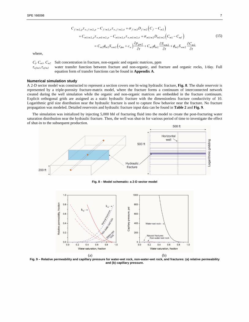
equation form of transfer functions can be found in Appendix A. Numerical simulation study A 2-D sector model was constructed to represent a section covers one bi-wing hydraulic fracture, Fig. 8. The shale reservoir is represented by a triple-porosity fracture-matrix model, where the fracture forms a continuum of interconnected network created during the well simulation while the organic and non-organic matrices are embedded in the fracture continuum. Explicit orthogonal grids are assigned as a static hydraulic fracture with the dimensionless fracture conductivity of 10. Logarithmic grid size distribution near the hydraulic fracture is used to capture flow behavior near the fracture. No fracture propagation was modeled. Detailed reservoirs and hydraulic fracture input data can be found in Table 2 and Fig. 9.
The simulation was initialized by injecting 5,000 bbl of fracturing fluid into the model to create the post-fracturing water saturation distribution near the hydraulic fracture. Then, the well was shut-in for various period of time to investigate the effect of shut-in to the subsequent production.
Fig. 8 – Model schematic: a 2-D sector model
(a) (b)
Fig. 9 – Relative permeability and capillary pressure for water-wet rock, non-water-wet rock, and fractures: (a) relative permeability and (b) capillary pressure.
8 SPE 166098
TABLE 2 – INPUT PARAMETERS: A 2-D SECTOR MODEL
Parameter Natural fractures (f) Non-organic rock (m1)
Organic rock (m2)
Effective permeability, md 0.01 0.0001 0.0001
Effective porosity, fraction 0.0015 0.054 0.030
Irreducible water saturation, fraction 0.05 0.40 (water-wet) 0.05 (non-water-wet)
0.05
Capillary pressure at irreducible water saturation, psi
1.0 1000.0 (water-wet) 1.0 (non-water-wet)
10.0
Volume fraction, fraction - 0.9 0.1
Shape factor, 1/ft2 0.30 (f-m1) 0.10 (m1-m2) 0.03 (f-m2)
Salt diffusion coefficient, ft2/day 10-8 (f-m1) 10-8 (m1-m2) 10-8 (f-m2)
Formation brine salinity, ppm 150,000 150,000 150,000
Gas absorption coefficient Maximum gas absorption, scf/ton
n/a
n/a
2000*
Longmuir coefficient, 1/psi 0.00044
* Higher than a typical value because it only applies to the organic rock volume while the typical value is the weighted average absorption value for whole rocks including non-organic rock.
TABLE 3 – NUMERICAL SIMULATION CASES
Simulation
cases Pore fabric connection Osmotic
pressure
Non-organic rock
type
f-m1 f-m2 m1-m2 (a) WW+OSP √ √ √ √ Water-wet rock
(b) NW+OSP √ √ √ √ Non-water-wet rock
(c) WW+NOOSP √ √ √ Water-wet rock
(d) NW+NOOSP √ √ √ Non-water-wet rock
To investigate the role of matrix wettability, capillary pressure, relative permeability characteristics, and osmotic pressure, four simulation cases were run. Each case represents different combination of rock matrix wettability including water-wet and non-water-wet rock, and the presence of osmotic pressure. The summary of simulation cases is shown in Table 3. Different shut-in periods including 0, 7, 15, and 30 days shut-in period, were included in the simulation cases.
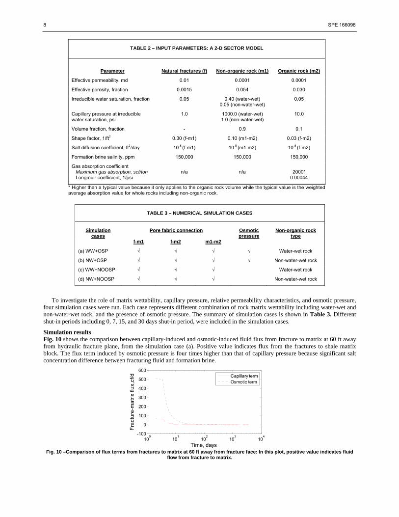
Simulation results Fig. 10 shows the comparison between capillary-induced and osmotic-induced fluid flux from fracture to matrix at 60 ft away from hydraulic fracture plane, from the simulation case (a). Positive value indicates flux from the fractures to shale matrix block. The flux term induced by osmotic pressure is four times higher than that of capillary pressure because significant salt concentration difference between fracturing fluid and formation brine.
Fig. 10 –Comparison of flux terms from fractures to matrix at 60 ft away from fracture face: In this plot, positive value indicates fluid
flow from fracture to matrix.
100
101
102
103
104
-100
0
100
200
300
400
500
600
Time, days
Fra
ctu
re-m
atr
ix fl
ux,
cf/d
Capillary termOsmotic term
SPE 166098 9
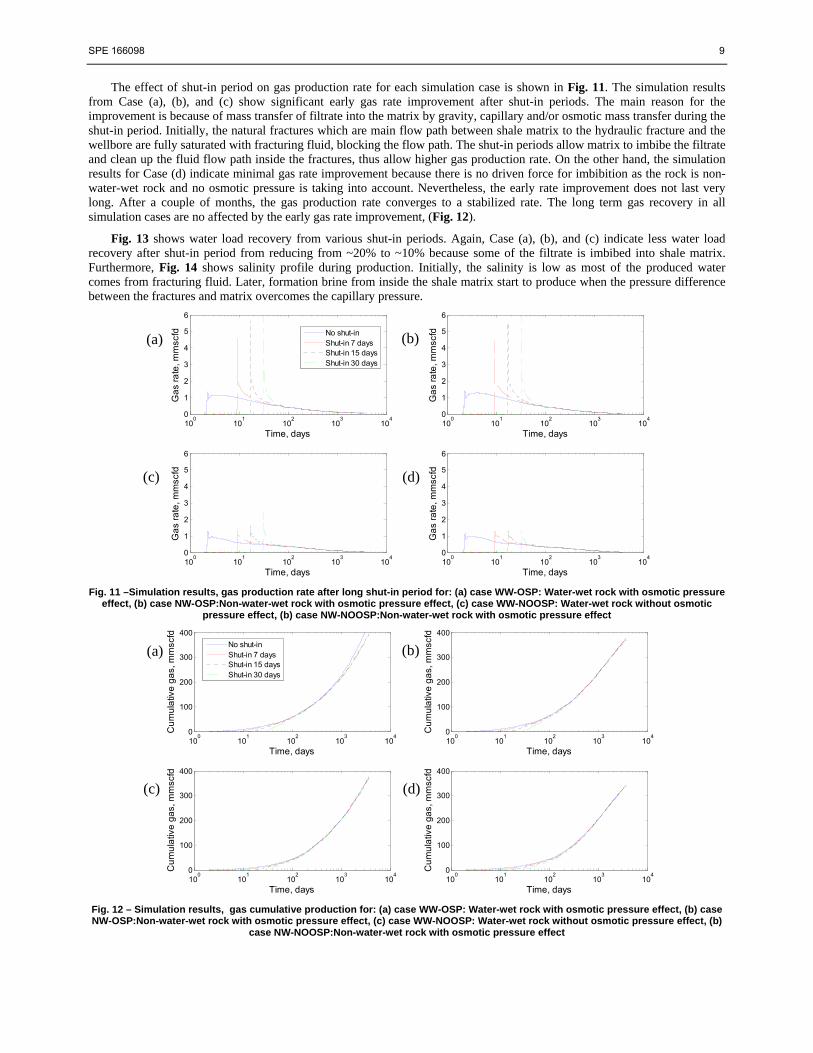
The effect of shut-in period on gas production rate for each simulation case is shown in Fig. 11. The simulation results from Case (a), (b), and (c) show significant early gas rate improvement after shut-in periods. The main reason for the improvement is because of mass transfer of filtrate into the matrix by gravity, capillary and/or osmotic mass transfer during the shut-in period. Initially, the natural fractures which are main flow path between shale matrix to the hydraulic fracture and the wellbore are fully saturated with fracturing fluid, blocking the flow path. The shut-in periods allow matrix to imbibe the filtrate and clean up the fluid flow path inside the fractures, thus allow higher gas production rate. On the other hand, the simulation results for Case (d) indicate minimal gas rate improvement because there is no driven force for imbibition as the rock is non-water-wet rock and no osmotic pressure is taking into account. Nevertheless, the early rate improvement does not last very long. After a couple of months, the gas production rate converges to a stabilized rate. The long term gas recovery in all simulation cases are no affected by the early gas rate improvement, (Fig. 12).
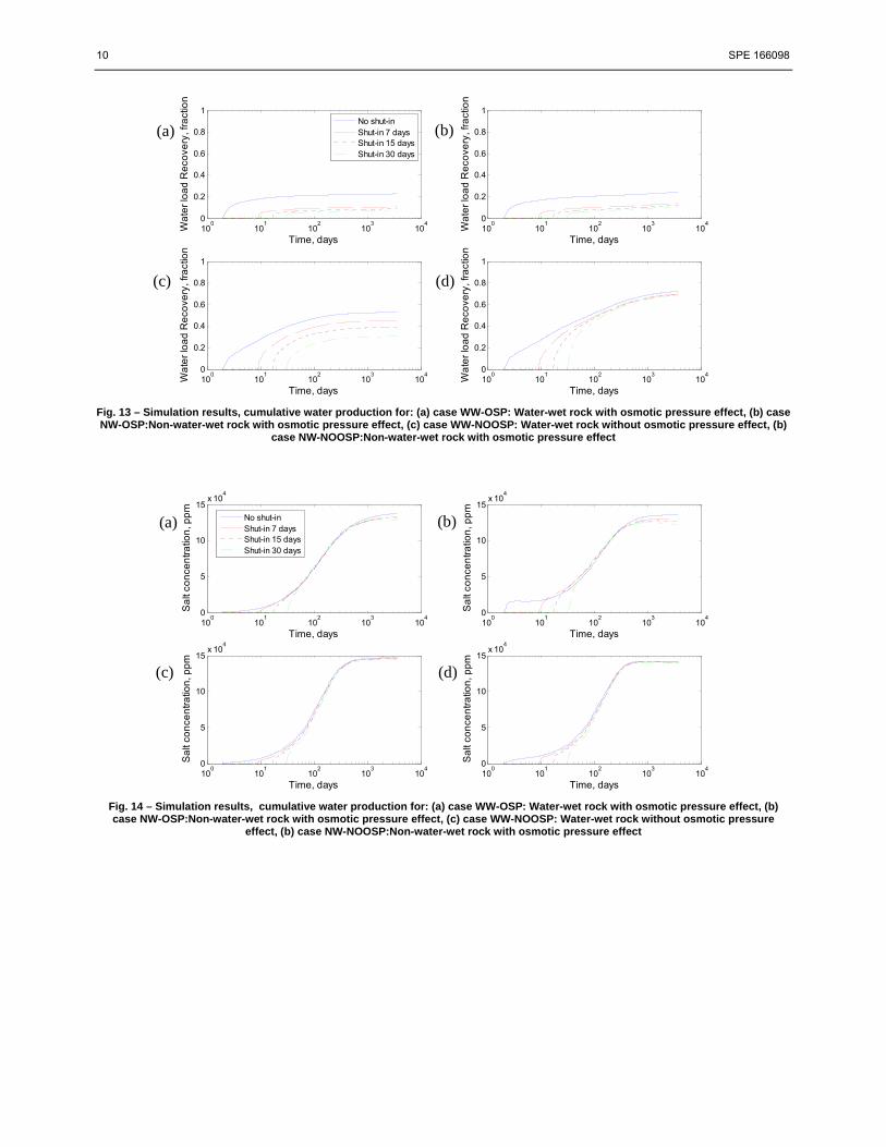
Fig. 13 shows water load recovery from various shut-in periods. Again, Case (a), (b), and (c) indicate less water load recovery after shut-in period from reducing from ~20% to ~10% because some of the filtrate is imbibed into shale matrix. Furthermore, Fig. 14 shows salinity profile during production. Initially, the salinity is low as most of the produced water comes from fracturing fluid. Later, formation brine from inside the shale matrix start to produce when the pressure difference between the fractures and matrix overcomes the capillary pressure.
Fig. 11 –Simulation results, gas production rate after long shut-in period for: (a) case WW-OSP: Water-wet rock with osmotic pressure
effect, (b) case NW-OSP:Non-water-wet rock with osmotic pressure effect, (c) case WW-NOOSP: Water-wet rock without osmotic pressure effect, (b) case NW-NOOSP:Non-water-wet rock with osmotic pressure effect
Fig. 12 – Simulation results, gas cumulative production for: (a) case WW-OSP: Water-wet rock with osmotic pressure effect, (b) case NW-OSP:Non-water-wet rock with osmotic pressure effect, (c) case WW-NOOSP: Water-wet rock without osmotic pressure effect, (b)
case NW-NOOSP:Non-water-wet rock with osmotic pressure effect
100
101
102
103
104
0
1
2
3
4
5
6
Time, days
Ga
s ra
te, m
msc
fd
No shut-inShut-in 7 daysShut-in 15 daysShut-in 30 days
100
101
102
103
104
0
1
2
3
4
5
6
Time, daysG
as
rate
, mm
scfd
100
101
102
103
104
0
1
2
3
4
5
6
Time, days
Ga
s ra
te, m
msc
fd
100
101
102
103
104
0
1
2
3
4
5
6
Time, days
Ga
s ra
te, m
msc
fd
100
101
102
103
104
0
100
200
300
400
Time, days
Cu
mu
lativ
e g
as,
mm
scfd
No shut-inShut-in 7 daysShut-in 15 daysShut-in 30 days
100
101
102
103
104
0
100
200
300
400
Time, days
Cu
mu
lativ
e g
as,
mm
scfd
100
101
102
103
104
0
100
200
300
400
Time, days
Cu
mu
lativ
e g
as,
mm
scfd
100
101
102
103
104
0
100
200
300
400
Time, days
Cu
mu
lativ
e g
as,
mm
scfd
(a) (b)
(c) (d)
(a) (b)
(c) (d)
10 SPE 166098
Fig. 13 – Simulation results, cumulative water production for: (a) case WW-OSP: Water-wet rock with osmotic pressure effect, (b) case NW-OSP:Non-water-wet rock with osmotic pressure effect, (c) case WW-NOOSP: Water-wet rock without osmotic pressure effect, (b)
case NW-NOOSP:Non-water-wet rock with osmotic pressure effect
Fig. 14 – Simulation results, cumulative water production for: (a) case WW-OSP: Water-wet rock with osmotic pressure effect, (b) case NW-OSP:Non-water-wet rock with osmotic pressure effect, (c) case WW-NOOSP: Water-wet rock without osmotic pressure
effect, (b) case NW-NOOSP:Non-water-wet rock with osmotic pressure effect
100
101
102
103
104
0
0.2
0.4
0.6
0.8
1
Time, days
Wa
ter
loa
d R
eco
very
, fra
ctio
n
No shut-inShut-in 7 daysShut-in 15 daysShut-in 30 days
100
101
102
103
104
0
0.2
0.4
0.6
0.8
1
Time, days
Wa
ter
loa
d R
eco
very
, fra
ctio
n
100
101
102
103
104
0
0.2
0.4
0.6
0.8
1
Time, days
Wa
ter
loa
d R
eco
very
, fra
ctio
n
100
101
102
103
104
0
0.2
0.4
0.6
0.8
1
Time, days
Wa
ter
loa
d R
eco
very
, fra
ctio
n
100
101
102
103
104
0
5
10
15x 10
4
Time, days
Sa
lt co
nce
ntr
atio
n, p
pm
No shut-inShut-in 7 daysShut-in 15 daysShut-in 30 days
100
101
102
103
104
0
5
10
15x 10
4
Time, days
Sa
lt co
nce
ntr
atio
n, p
pm
100
101
102
103
104
0
5
10
15x 10
4
Time, days
Sa
lt co
nce
ntr
atio
n, p
pm
100
101
102
103
104
0
5
10
15x 10
4
Time, days
Sa
lt co
nce
ntr
atio
n, p
pm
(a) (b)
(c) (d)
(a) (b)
(c) (d)
SPE 166098 11
Conclusions In this paper, we report the development of a mathematical model to include gravity, capillary, and osmotic pressure effects
in a triple-porosity system for organic-rich shale formations. The osmotic pressure model is based on experimental data. We also conducted the numerical experiments to investigate the effect of the post-fracturing long shut-in periods on the initial gas production rate and fracturing fluid recovery. The following conclusion can be drawn from the simulation results:
1. We have been able to simulate the effect of shut-in of newly created hydraulic fractures on increased production
of gas in organic-rich shale reservoirs. The results are similar with field data reported in literature.
2. The reason for the increase in gas production is because of mass transfer of filtrate into the matrix by gravity, capillary and/or osmotic mass transfer during the shut-in period, which reduces the liquid saturation in natural fractures and allows gas to flow at higher rates from the fractures.
3. The rate increase is not a lasting effect and depends on the nature of pore connectivity.
Acknowledgement This work is supported by the U.S. Department of Energy under Contract No. DE-EE0002762. Special thanks are due to Energy Modeling Group (EMG) and Marathon Center of Excellence for Reservoir Studies (MCERS) at Colorado School of Mines. Nomenclature
Ia water activity of system I, dimensionless
c compressibility, 1/psi C salt concentration, ppm D depth, ft Df/m diffusion coefficient between fracture and matrix, ft2/day k permeability, md p pressure, psi q̂ sink/source term, 1/day
R gas constant, equal to 0.082 atm. (mol.K)-1 t time, day T temperature, K V partial molar volume, l/mol Greek letter porosity, fraction fluid gradient, psi/ft mobility, 1/cp viscosity, cp osmotic pressure, psi transfer function, 1/day Subscript eff effective f fracture f/m1 between fracture and non-organic matrix f/m2 between fracture and organic matrix g gas phase m1/m2 between non-organic and organic matrices m1, m2 non-organic and organic matrices p pressure term t total phase w water phase osmotic pressure term
12 SPE 166098
References Al-Bazali, T. M., J. Zhang, M. E. Chenevert, and M. M. Sharma, 2006, “Factors Controlling the Membrane Efficiency of
Shales When Interacting With Water-Based and Oil-Based Muds,” In International Oil & Gas Conference and Exhibition in China. Beijing, China: Society of Petroleum Engineers.
Barry, T. H., R. K. Meyer, K. Yule, and J. Wittenberg, 2012, “A Case for Oil-Based Fracturing Fluids in Canadian Montney
Unconventional Gas Development” In SPE Annual Technical Conference and Exhibition, San Antonio, Texas, USA: Society of Petroleum Engineers.
Bredehoeft, J. D., C. R. Blyth, W. A. White, and G. B. Maxey, 1963, “Possible Mechanism for Concentration of Brines in
Subsurface Formations.” AAPG Bulletin 47, no. 2: 257–269. Cheng, Y., 2012, “Impact of Water Dynamics in Fractures on the Performance of Hydraulically Fractured Wells in Gas-Shale
Reservoirs.” Journal of Canadian Petroleum Technology 51, no. 2: pp. 143–151. Economides, C. A., I. A. Ahmed, S. Apiwathanasorn, J. H. Lightner, B. Song, F. E. Vera Rosales, H. Xue, and Y. Zhang,
2012, “Stimulated Shale Volume Characterization: Multiwell Case Study from the Horn River Shale: II. Flow Perspective” In SPE Annual Technical Conference and Exhibition, San Antonio, Texas, USA: Society of Petroleum Engineers.
Haluszczak, L. O., A. W. Rose, and L. R. Kump, 2013, “Geochemical Evaluation of Flowback Brine from Marcellus Gas
Wells in Pennsylvania, USA,” Applied Geochemistry 28: 55–61, doi:10.1016/j.apgeochem.2012.10.002. Kazemi, H., S. Atan, M. Al-Matrook, J. Dreier, and E. Ozkan, 2005, “Multilevel Fracture Network Modeling of Naturally
Fractured Reservoirs.” In SPE Reservoir Simulation Symposium, The Woodlands, Texas. King, G. E., 2012, “Hydraulic Fracturing 101: What Every Representative, Environmentalist, Regulator, Reporter, Investor,
University Researcher, Neighbor and Engineer Should Know About Estimating Frac Risk and Improving Frac Performance in Unconventional Gas and Oil Wells,” In SPE Hydraulic Fracturing Technology Conference. The Woodlands, Texas, USA: Society of Petroleum Engineers.
Lane, R., and A. Aderibigbe, 2013, “Rock/Fluid Chemistry Impacts on Shale Fracture Behavior,” In 2013 SPE International
Symposium on Oilfield Chemistry, The Woodlands, TX, USA: Society of Petroleum Engineers. Marine, I. W., and S. J. Fritz, 1981, “Osmotic Model to Explain Anomalous Hydraulic Heads,” Water Resources Research 17,
no. 1: 73–82. doi:10.1029/WR017i001p00073. Neuzil, C. E., and A. M. Provost, 2009, “Recent Experimental Data May Point to a Greater Role for Osmotic Pressures in the
Subsurface,” Water Resources Research, 45, no. 3, doi:10.1029/2007WR006450. Neuzil, C. E, 2000, “Osmotic Generation of ‘anomalous’ Fluid Pressures in Geological Environments,” Nature, 403, no. 6766:
182–184, doi:10.1038/35003174. Parmar, J., H. Dehghanpour and E. Kuru, 2013, “Drainage Against Gravity: Factors Impacting the Load Recovery in
Fractures,” In SPE Unconventional Resources Conference, The Woodlands, TX, USA: Society of Petroleum Engineers. Passey, Q. R., K. Bohacs, W. L. Esch, R. Klimentidis, and S. Sinha, 2010, “From Oil-Prone Source Rock to Gas-Producing
Shale Reservoir – Geologic and Petrophysical Characterization of Unconventional Shale-Gas Reservoirs,” In International Oil and Gas Conference and Exhibition in China. Beijing, China: Society of Petroleum Engineers.
Xu, T., N. Spycher, E. Sonnenthal, G. Zhang, L. Zheng, and K. Pruess, 2012, “TOUGHREACT User’s Guide: A Simulator
Program for Non-isothermal Multiphase Reactive Transport in Variably Saturated Geological Media, Version 2.0.”
SPE 166098 13
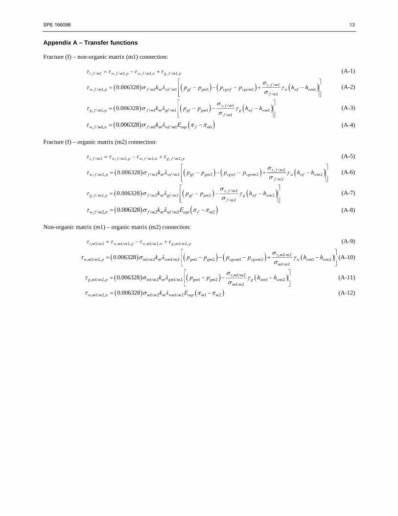
Appendix A – Transfer functions
Fracture (f) – non-organic matrix (m1) connection:
, / 1 , / 1, , / 1, , / 1,t f m w f m p w f m g f m p (A-1)
, / 1, / 1, / 1 / 1 1 1 1
/ 1
0.006328 z f mw f m p f m m wf m gf gm cgwf cgwm w wf wm
f m
k p p p p h h
(A-2)
, / 1, / 1, / 1 / 1 1 1
/ 1
0.006328 z f mg f m p f m m gf m gf gm g wf wm
f m
k p p h h
(A-3)
, / 1, / 1 / 1 10.006328w f m f m m wf m osp f mk E (A-4)
Fracture (f) – organic matrix (m2) connection:
, / 2 , / 2, , / 2, , / 2,t f m w f m p w f m g f m p (A-5)
, / 2, / 2, / 2 / 2 2 2 2
/ 2
0.006328 z f mw f m p f m m wf m gf gm cgwf cgwm w wf wm
f m
k p p p p h h
(A-6)
, / 2, / 2, / 2 / 2 2 2
/ 2
0.006328 z f mg f m p f m m gf m gf gm g wf wm
f m
k p p h h
(A-7)
, / 2, / 2 / 2 20.006328w f m f m m wf m osp f mk E (A-8)
Non-organic matrix (m1) – organic matrix (m2) connection:
, 1/ 2 , 1/ 2, , 1/ 2, , 1/ 2,t m m w m m p w m m g m m p (A-9)
, 1/ 2, 1/ 2, 1/ 2 1/ 2 1 2 1 2 1 2
1/ 2
0.006328 z m mw m m p m m m wm m gm gm cgwm cgwm w wm wm
m m
k p p p p h h
(A-10)
, 1/ 2, 1/ 2, 1/ 2 1/ 2 1 2 1 2
1/ 2
0.006328 z m mg m m p m m m gm m gm gm g wm wm
m m
k p p h h
(A-11)
, 1/ 2, 1/ 2 1/ 2 1 20.006328w m m m m m wm m osp m mk E (A-12)