Copyright 2007, Society of Petroleum Engineers This paper was prepared for presentation at the 2007 SPE Annual Technical Conference and Exhibition held in Anaheim, California, U.S.A., 11–14 November 2007. This paper was selected for presentation by an SPE Program Committee following review of information contained in an abstract submitted by the author(s). Contents of the paper, as presented, have not been reviewed by the Society of Petroleum Engineers and are subject to correction by the author(s). The material, as presented, does not necessarily reflect any position of the Society of Petroleum Engineers, its officers, or members. Papers presented at SPE meetings are subject to publication review by Editorial Committees of the Society of Petroleum Engineers. Electronic reproduction, distribution, or storage of any part of this paper for commercial purposes without the written consent of the Society of Petroleum Engineers is prohibited. Permission to reproduce in print is restricted to an abstract of not more than 300 words; illustrations may not be copied. The abstract must contain conspicuous acknowledgment of where and by whom the paper was presented. Write Librarian, SPE, P.O. Box 833836, Richardson, TX 75083-3836, U.S.A., fax 01-972-952-9435.

Abstract Probe-type formation testers are often used to estimate permeability and permeability anisotropy from pressure transient measurements. The interpretation of these measurements is not trivial in the presence of oil-base mud-filtrate invasion due to miscibility with formation oil and gas. Simple analytical expressions of spherical and linear single-phase flow may not give correct estimates of permeability in miscible or partially miscible flow regimes. A computationally demanding three-dimensional (3D) numerical model is required to provide accurate and reliable estimates of formation properties. Because pressure transients are nonlinearly dependent on the permeability of the formation, repeated 3D numerical simulations are necessary to match the measured pressure transients. We describe the development and successful implementation of a new inversion method that efficiently estimates permeability and permeability anisotropy with a cascade sequence of least-squares minimizations. Measurements consist of pressure transients acquired at the sand face with a probe-type wireline formation tester (WFT). The new inversion method executes the forward 3D problem only in an outer loop. In the inner loop, we perform fast minimizations with an equivalent two-dimensional (2D) cylindrical grid. Transient measurements of pressure at the sand face simulated with the 2D cylindrical grid are correlated to the corresponding measurements simulated with the 3D grid. Once the 2D minimization is completed, we perform a 3D simulation of transient pressure to update the 2D-3D correlation parameter and a new 2D minimization is performed until convergence is reached. The process repeats itself until the simulated 3D pressure transients reproduce the field measurements within pre-stipulated error bounds.

We perform tests of the new inversion algorithm on synthetic and field data sets acquired in the presence of oil-base mud-filtrate invasion. Results successfully confirm that our coupled 2D/3D hybrid inversion approach enables significant savings in computer time and provides reliable and accurate estimates of permeability and anisotropy. In most cases, we are able to estimate permeability under 2% error within 20% of the computational time required by 3D minimization. Sensitivity analysis indicates that permeability estimates may be biased by noisy measurements and uncertainty in (a) flow rates, (b) relative permeability, (c) radial extent of invasion, (d) formation damage, and (e) location of bed boundaries. Introduction

Formation testers are widely used to measure pressure and to estimate permeability from pressure transient measurements acquired with sink and observation probes. Often, WFT measurements remain influenced by the process of mud-filtrate invasion that takes place prior to measurement acquisition.1,2 Mud-filtrate invasion makes it inadequate to use single-phase analytical solutions of pressure transient measurements to estimate permeability. Commercial pressure-transient interpretation methods take invasion into account by invoking a dynamic skin factor. Typically, these methods estimate permeability by neglecting early-time pressure data that are attributed to noisy measurements. However, previous studies on formation testing have shown that early-time pressure measurements can provide useful information about both radial extent of mud-filtrate invasion2 and relative permeability3,4. Formation-testing measurements can also be integrated into reservoir models to diagnose and quantify spatial variations of permeability. Therefore, it is important to use a 3D numerical model to simulate measurements acquired with probe-type WFT in order to obtain reliable estimates of formation permeability, radial extent of invasion, relative permeability, location of layers, and for integration with an underlying geological model. However, such an exercise entails executing a computationally intensive 3D numerical simulation of the forward model to invert for permeability. A hybrid inversion technique can be useful to decrease computer times without compromising the accuracy and reliability of the permeability estimates.

SPE 109956

A dual-grid automatic history matching technique with applications to 3D formation testing in the presence of oil-base muds Mayank Malik, Carlos Torres-Verdín, and Kamy Sepehrnoori, The University of Texas at Austin

2 SPE 109956

Torres-Verdín et al.5 successfully implemented a dual-grid cascade sequence of minimizations to invert cross- and single-well direct-current (dc) resistivity measurements into 2D spatial distributions of electrical conductivity. Using a forward model as an approximation to the model used to acquire the measurements, they were able to solve the inversion problem with significant savings in computer time. They also advanced a proof of convergence for the hybrid minimization method. In this paper, we use a similar inversion method to estimate permeability and permeability anisotropy from transient pressure measurements acquired with a probe-type WFT. The method neglects azimuthal variations of permeability but does take into account the 3D spatial distribution of pressure within the formation. This assumption is not restrictive in field applications of WFT considering that, in general, azimuthal permeability is the same as radial permeability. Our dual grid consists of (a) 3D grid that models the probe geometry, and (b) a 2D axi-symmetric grid. For the same assumed flow rates of fluid withdrawal, the simulated 2D and 3D pressure transients are different in the corresponding grids because of the difference of surface area of probe opening in the two cases. To circumvent this problem, we correlate the transient pressure measurements simulated separately with the 2D and 3D grids. Upon obtaining the correlation parameter between the two sets of simulations, we only use the 2D grid for minimization.

Due to the complexity of miscible flow in the formation, limited work has been advanced to simulate formation-tester measurements in the presence of oil-base muds (OBM). McCalmont et al.6 performed sensitivity analyses to determine pumpout volume for gas condensates using an immiscible flow formulation. Alpak et al.2 used a miscible flow approach with a compositional equation-of-state (EOS) simulator and compared field measurements of gas/oil ratio (GOR) to their simulated GOR estimates. However, their work lacked comparisons of field measurements of probe pressure against numerical simulations. Angeles et al.7 described applications of a least-squares inversion technique that was used to estimate permeability from transient pressure measurements acquired with a packer-type WFT. Wu et al.8 used a commercial compositional simulator with a binary component formulation to estimate permeability using a neural network approach.

In this paper, we simulate displacement of multi-component OBMs and formation oil in porous media with a compositional EOS simulator (CMG-GEM‡9). The unknown inversion parameters are formation permeability and permeability anisotropy. Our compositional model consists of eight pseudo-components: five formation oil components and three oil-base mud-filtrate components, included to accurately model the time-space evolution of miscible flow. Hydrocarbon phase compositions are tracked using the Peng-Robinson10 EOS. Phase density is calculated from the EOS to account for variations of fluid density due to changes of pressure and fluid composition. Similarly, fluid viscosity is calculated from the Lohrenz-Bray-Clark11 (LBC) correlation to account for time- ‡ Copyright of Computer Modeling Group Limited

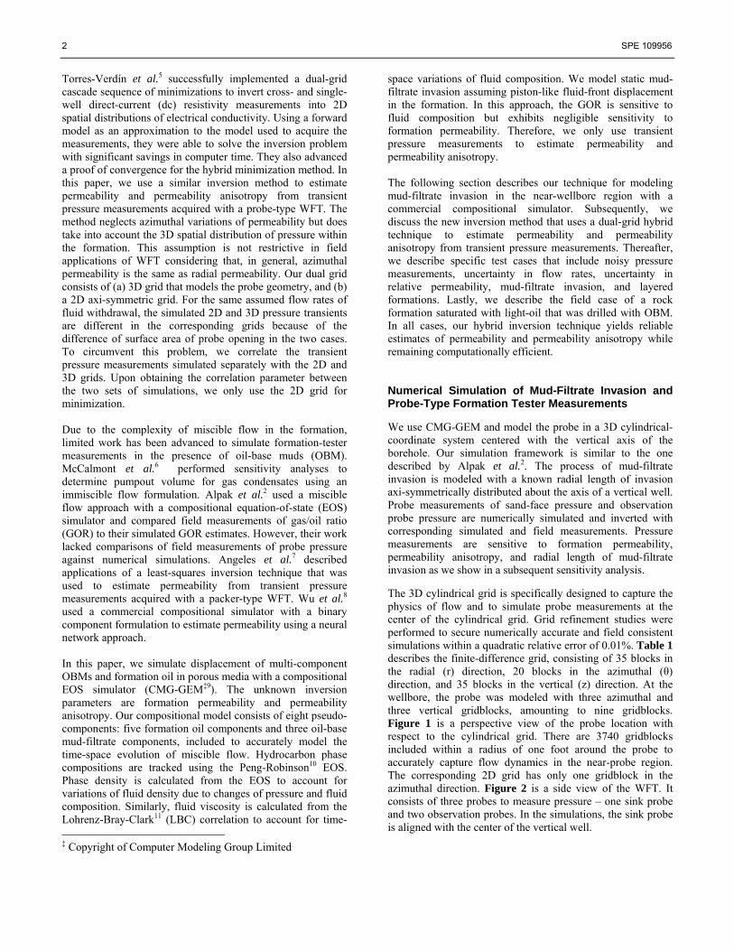
space variations of fluid composition. We model static mud-filtrate invasion assuming piston-like fluid-front displacement in the formation. In this approach, the GOR is sensitive to fluid composition but exhibits negligible sensitivity to formation permeability. Therefore, we only use transient pressure measurements to estimate permeability and permeability anisotropy. The following section describes our technique for modeling mud-filtrate invasion in the near-wellbore region with a commercial compositional simulator. Subsequently, we discuss the new inversion method that uses a dual-grid hybrid technique to estimate permeability and permeability anisotropy from transient pressure measurements. Thereafter, we describe specific test cases that include noisy pressure measurements, uncertainty in flow rates, uncertainty in relative permeability, mud-filtrate invasion, and layered formations. Lastly, we describe the field case of a rock formation saturated with light-oil that was drilled with OBM. In all cases, our hybrid inversion technique yields reliable estimates of permeability and permeability anisotropy while remaining computationally efficient. Numerical Simulation of Mud-Filtrate Invasion and Probe-Type Formation Tester Measurements We use CMG-GEM and model the probe in a 3D cylindrical-coordinate system centered with the vertical axis of the borehole. Our simulation framework is similar to the one described by Alpak et al.2. The process of mud-filtrate invasion is modeled with a known radial length of invasion axi-symmetrically distributed about the axis of a vertical well. Probe measurements of sand-face pressure and observation probe pressure are numerically simulated and inverted with corresponding simulated and field measurements. Pressure measurements are sensitive to formation permeability, permeability anisotropy, and radial length of mud-filtrate invasion as we show in a subsequent sensitivity analysis. The 3D cylindrical grid is specifically designed to capture the physics of flow and to simulate probe measurements at the center of the cylindrical grid. Grid refinement studies were performed to secure numerically accurate and field consistent simulations within a quadratic relative error of 0.01%. Table 1 describes the finite-difference grid, consisting of 35 blocks in the radial (r) direction, 20 blocks in the azimuthal (θ) direction, and 35 blocks in the vertical (z) direction. At the wellbore, the probe was modeled with three azimuthal and three vertical gridblocks, amounting to nine gridblocks. Figure 1 is a perspective view of the probe location with respect to the cylindrical grid. There are 3740 gridblocks included within a radius of one foot around the probe to accurately capture flow dynamics in the near-probe region. The corresponding 2D grid has only one gridblock in the azimuthal direction. Figure 2 is a side view of the WFT. It consists of three probes to measure pressure – one sink probe and two observation probes. In the simulations, the sink probe is aligned with the center of the vertical well.

SPE 109956 3

FIG. 1 Three-dimensional view of the sink probe opening with respect to a cylindrical finite-difference grid. The probe opening is highlighted with a red dot. Note that the region around the probe opening is discretized in all directions (r,θ,z) to accurately simulate transient measurements of pressure, flow rate, and GOR. The corresponding 2D simulation grid includes only one gridblock in the azimuthal direction thereby neglecting azimuthal variations of permeability, porosity, pressure, and molar concentrations.

2.3 ft

8 ft

SINK PROBE

OBSERVATION PROBE 1

OBSERVATIONPROBE 2

FIG. 2 Configuration of the probe-type wireline formation tester consisting of two vertical observation probes and one sink probe. The sink probe is located at the center of the numerical grid for all the simulations described in the paper.

TABLE 1: Summary of geometrical and numerical simulation parameters assumed for all 3D grid cases considered in this paper. The corresponding 2D grid neglects formation and fluid property variations in the azimuthal direction. Parameter Units Value Wellbore radius (rw) ft 0.55 External radius (re) ft 300 Reservoir thickness ft 41.75 Number of nodes – radial axis -- 35 Number of nodes – azimuthal axis -- 20 Number of nodes – vertical axis -- 35 Grid cell size – r ft Variable Grid cell size – θ degrees Variable Grid cell size – z ft Variable

Previous studies that simulated probe dynamics assumed a symmetric geometry in the azimuthal direction and modeled only half of the probe to reduce computer time2,6. Here, we use a full 3D grid geometry and make no restrictive assumptions about spatial symmetry. In order to decrease computer time, we use a 180-degree azimuthal gridblock behind the probe. This grid selection is in agreement with our observations that the pressure differential is higher in the region in front of the probe than in the region behind the probe. Thus, a coarser 180-degree gridblock can be used to accurately model the geometry without entailing boundary effects (as could be the case when assuming symmetry and modeling the probe at the corner of the computational grid).

The process of mud-filtrate invasion is modeled with a known radial length of invasion around the near-wellbore region. We assume that invasion is axi-symmetric and initialize the near-wellbore region with component concentrations of the oil-base mud in our 3D grid model. Simulated transient pressure measurements are sensitive to radial length of invasion as OBM viscosity differs from formation oil viscosity. Although both oil-base mud filtrate and reservoir oil constitute the same phase, their viscosity and density contrasts affect pressure transients at early times when mud filtrate contaminates the near-probe region. We use actual field data to assign component concentrations to formation hydrocarbons and OBM in our simulations. Based on PVT reports from laboratory analysis of samples, formation hydrocarbons consist of components in the range from C1 to C19+. Formation hydrocarbons are lumped into five different components (N2C1, CO2C3, C4C6, C7C18, and C19+) using their pseudo-physical properties summarized in Table 3. Oil-base mud composition is lumped into three other components (MC14, MC16, and MC18), as shown in Table 4. Therefore, our compositional simulations consist of eight different hydrocarbon pseudo-components. Such reduction of the number of components is necessary to decrease the computer run time. Before accepting the proposed fluid compositional breakdown, we performed quality check against the measured PVT data and proved that the proposed eight-component fluid model properly accounted for density and viscosity changes (and other key parameters such as GOR and liberated gas volumes) due to variations of component concentrations and pressure. Our formulation enforces boundary and source flow-rate conditions on specific depth segments along the wellbore. At the wellbore, the WFT imposes a constant flow rate condition during fluid production. Probe opening is modeled as a source or a well spread over nine gridblocks (three azimuthal and three vertical blocks) with a diameter of approximately one inch. The outer limits of the reservoir consist of impermeable terminations with no-flow boundary conditions.

4 SPE 109956

TABLE 2: Summary of the assumed petrophysical and fluid properties for all simulation cases. Property Units Value Initial water saturation fraction 0.22 Water Compressibility 1/psi 3e-6 Formation porosity fraction 0.18 Temperature Fahrenheit 140 Formation compressibility 1/psi 1e-9 Reservoir oil density g/cc 0.60 Reservoir oil viscosity cp 0.36 Clean gas-oil ratio SCF/STB 2193

TABLE 3: Equation-of-state parameters and mole fractions of the pseudo-components used in this paper to describe the behavior of in-situ fluids. Parameter N2 C1 CO2 C3 C4 C6 C7 C18 C19+ Molar Concentration 0.6183 0.0792 0.0875 0.1786 0.0362

Critical Temperature (oF)

-125.7 125.9 359.8 656.2 1059.9

Critical Pressure (psi) 653.3 839.4 498.2 322.3 184.4

Acentric Factor 0.0105 0.1458 0.2302 0.4904 0.9192

Molar Weight (lbs/ moles) 16.6 36.23 67.73 132.79 303.21

Volume Shift Parameter -0.193 -0.131 -0.056 0.171 0.231

TABLE 4: Equation-of-state parameters and mole fractions of the pseudo-components used in this paper to describe the behavior of oil-base mud. Parameter MC14 MC16 MC18 Molar Concentration 0.6489 0.2145 0.1364

Critical Temperature (oF) 755.1 822.5 878.1

Critical Pressure (psi) 261.8 240.2 224.4

Acentric Factor 0.6257 0.7118 0.7842 Molar Weight (lbs/ moles) 190 222 251

Volume Shift Parameter 0.0792 0.0666 0.0439

Table 5: Summary of petrophysical, formation, and simulation parameters for the base-case formation model. Parameter Units Value Horizontal Permeability mD 200 Vertical Permeability mD 67 Porosity - 0.18 Test Duration sec 4320 Probe Flow rate barrels/day 12-18 Irreducible Water Saturation - 0.22 Radial length of invasion inches 0

FIG. 3 Water-oil relative permeability and capillary pressure curves assumed in the numerical simulation of formation-tester measurements described in this paper.

Base Case Model Table 5 summarizes the petrophysical, formation, and numerical simulation properties for the base case simulation model. We assume a homogeneous, single-layer anisotropic formation as our base case model.

Figure 3 shows the assumed saturation-dependent Brooks-Corey12 relative permeability and drainage capillary pressure curves. The irreducible water saturation is 0.22, whereas the simulated production time is 3600 sec and buildup time is 504 sec. Rate of fluid pumpout is 12 RB/day for the first 1800 sec of production and 18 RB/day for the subsequent 1800 sec. Total fluid pumpout volume is 0.625 barrels. Nonlinear Inversion Algorithm For inversion, we implement the general nonlinear least-squares minimization method described by Madsen et al.16. The following sub-sections describe our inversion algorithm as implemented to interpret formation-tester measurements. We describe the cost function that is composed of transient pressure measurements at the sand face and at the observation probes. Subsequently, we discuss the Levenberg-Marquardt13,14 algorithm that is used to estimate permeability and permeability anisotropy from transient pressure measurements. In the next sub-section, we introduce a hybrid grid technique that uses 2D simulations to approximate 3D probe measurements. Then, Cramer-Rao17 bounds are introduced to quantify confidence bounds in the estimated values of permeability and permeability anisotropy from noisy measurements. Lastly, we describe some features specific to the CMG-GEM simulator that significantly improve the efficiency of the hybrid minimization method. Cost Function Given a vector residual function : n m→e with m n≥ , the cost function ( ( ))C x is defined as

2

1

1 1( ) ( ( )) ( ) ( )2 2

i m

ii

C e=

Τ

=

= =∑x x e x e x , …(1)

where m is the length of the model vector and n is the length of the data vector. There are m time samples of pressure measurements and n unknown parameters in equation 1. The factor ½ in the above equation is introduced for convenience and has no effect on convergence. In formation testing applications, the model vector (x) typically describes the permeability tensor, which includes radial and vertical permeability. The dimensionless residual vector is the relative pressure difference between the simulated and the observed measurements, defined as

1 11( ) / ( ) 1( )

( ) / ( ) 1( ) ( )

( ) ( ) / ( ) 1

i i

m m

sim obs

sim obsi

m sim obs

p pe

p pe

e p p

−⎡ ⎤⎡ ⎤⎢ ⎥⎢ ⎥⎢ ⎥⎢ ⎥⎢ ⎥−⎢ ⎥= =⎢ ⎥⎢ ⎥⎢ ⎥⎢ ⎥⎢ ⎥⎢ ⎥ −⎣ ⎦ ⎣ ⎦

x xx

x xe x x

x x x

, …(2)

where subscript sim identifies the numerically simulated and obs identifies the observed transients, pressure measurements

SPE 109956 5

(p), respectively. Since we use 3 transient pressure probe measurements (sink probe and two observation probes), the data residual vector is concatenated with the three pressure vectors. In equation 1, the cost function is composed of the relative pressure difference and therefore its units are dimensionless. The inversion algorithm estimates permeability and permeability anisotropy, denoted by the vector x, by simultaneously honoring the three available pressure measurements of sink and two observation probes. We introduce a Jacobian matrix that contains, as entries, the first-order partial derivatives of the residual vector as

( )( ) ( )iij

j

ex∂

=∂

J x x , …(3)

where m n×∈J is the Jacobian matrix. The gradient of the cost function is given by

1( ) ( )

mi

iij j

eC ex x=

∂∂=

∂ ∂∑x x . …(4)

Thus, in vector notation, equation 4 can be written as ( ) ( ) ( )C Τ′ =x J x e x , …(5)

where superscript T refers to the transpose of the matrix. Similarly, the Hessian of the cost function is given by

1( ) ( ) ( ) ( ) ( )

m

i ii

C e x eΤ

=

′′ ′′= +∑x J x J x x . …(6)

We assume that the quadratic cost function ( ( ))C x is differentiable and smooth such that the Taylor series expansion gives

3( ) ( ) ( ) ( ) ( )C C OΤ Τ Τ= + +1x + h x h J x e x + h H x h ( h )2

, …(7)

where H is the Hessian matrix and h is a small perturbation on the model vector (x). In our implementation, we observed that the pressure output from CMG-GEM has only two decimal figures of precision. This numerical precision is inadequate for inversion, especially in high-porosity high-permeability formations when the pressure differential during drawdown and buildup is small. Extensive simulation exercises indicate that CMG-GEM allows six-decimal precision for pressure differential output and hence becomes better suitable for inversion. Therefore, instead of using the pressure output, we used the pressure differential from time zero. The residual based on pressure differential at the ith time step is given by

( ) ( ) / ( ) 1i ii sim obse p p= Δ Δ −x x x , …(8)

where i i op p pΔ = − is the pressure difference between the ith time step and the 0th time step. Moreover, the data residual vector includes pressure measurements acquired with both drawdown and the buildup periods. If the pressure differential is zero, the error function in equation 8 will tend to infinity. However, cases of zero pressure differential arise when the sand face pressure rises to the formation pressure (either before the sampling operation or at late times of buildup after sampling). In such cases, pressure is insensitive to variations of permeability. Therefore, we neglect pressure measurements acquired at those time steps when the pressure differential is less than 0.05 psi. Our

observation is that by performing this modification, we achieve better convergence and are successfully prevent the residual function from approaching infinity. Levenberg-Marquardt Minimization We use the Levenberg-Marquardt method for nonlinear minimization. This algorithm is a variation of the Gauss-Newton method with a damping parameter. Our minimization algorithm is based on the formulation given by Madsen et al.16 as ( ( ) ( ) ) ( ) ( )μΤ Τ+ = −J x J x I h J x e x , …(9) and damping or Lagrange parameter 0μ ≥ . In the above equation, I designates the identity matrix. For large values of μ , one has

( ) ( )μ

Τ

−J x e xh , …(10)

and is equivalent to a short step in the steepest-descent direction. For small values ofμ , equation 9 is equivalent to the Gauss-Newton method and provides quadratic convergence near the minima. At the outset, the initial μ relates to the size of the elements in the Jacobian matrix as

max { ( ) ( )}o iμ τ Τ= ⋅ o oJ x J x , …(11) where τ is a parameter that influences the convergence behavior in early iterations. Based on sensitivity analysis, we used a value of τ equal to 0.125 in all the inversion exercises reported in this paper. During subsequent iterations, μ varies depending on the norm of the Jacobian matrix. In order to decrease the computer time necessary to calculate the Jacobian matrix, we use Broyden’s15 secant updates, given by

11 1

{ ( ) ( ) ( ) }( ) ( ) k k kk k k k

++ + Τ

− −= + ⋅

e x e x J x hJ x J x hh h

, …(12)

where the subscript k identifies the iteration number. At the start of the minimization, we calculate the Jacobian matrix numerically by perturbing the model vector (x) by 0.5 mD. Subsequently, we only use Broyden’s updates to approximate the Jacobian matrix. Our observation is that Broyden’s updates are much cheaper computationally than calculating the Jacobian matrix at each iteration. In addition, the number of iterations required to reach the minimum with Broyden’s updates is similar to the number of iterations required to reach the minimum using Jacobian matrix calculations. There are instances in practical applications where the minimization algorithm converges to local minima and is unable to find a suitable direction that decreases the cost function for subsequent iterations. If this condition occurs for over 4 subsequent iterations, then we recalculate the Jacobian matrix numerically. Hybrid Inversion Technique We provide a systematic description of our hybrid inversion technique in this section. Underlying the algorithm is the assumption that we neglect azimuthal variations of permeability and porosity. Torres-Verdín et al.5 give a proof of convergence of the hybrid minimization technique.

6 SPE 109956

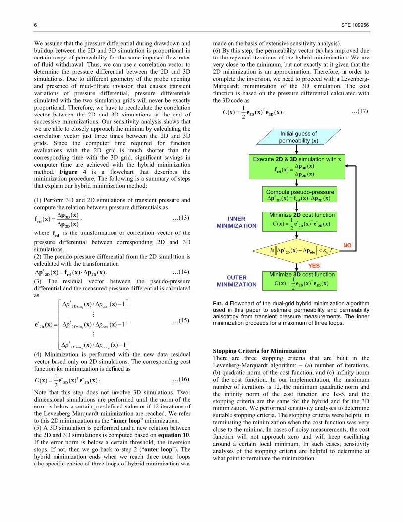
We assume that the pressure differential during drawdown and buildup between the 2D and 3D simulation is proportional in certain range of permeability for the same imposed flow rates of fluid withdrawal. Thus, we can use a correlation vector to determine the pressure differential between the 2D and 3D simulations. Due to different geometry of the probe opening and presence of mud-filtrate invasion that causes transient variations of pressure differential, pressure differentials simulated with the two simulation grids will never be exactly proportional. Therefore, we have to recalculate the correlation vector between the 2D and 3D simulations at the end of successive minimizations. Our sensitivity analysis shows that we are able to closely approach the minima by calculating the correlation vector just three times between the 2D and 3D grids. Since the computer time required for function evaluations with the 2D grid is much shorter than the corresponding time with the 3D grid, significant savings in computer time are achieved with the hybrid minimization method. Figure 4 is a flowchart that describes the minimization procedure. The following is a summary of steps that explain our hybrid minimization method: (1) Perform 3D and 2D simulations of transient pressure and compute the relation between pressure differentials as

( )( )( )

Δ=Δ

3Drel

2D

p xf xp x

, …(13)

where relf is the transformation or correlation vector of the pressure differential between corresponding 2D and 3D simulations. (2) The pseudo-pressure differential from the 2D simulation is calculated with the transformation

( ) ( ) ( )∗Δ = ⋅Δ2D rel 2Dp x f x p x . …(14) (3) The residual vector between the pseudo-pressure differential and the measured pressure differential is calculated as

1 1

*2

*2

*2

( ) / ( ) 1

( ) / ( ) 1( )

( ) / ( ) 1

i i

m m

Dsim obs

Dsim obs

Dsim obs

p p

p p

p p

∗

⎡ ⎤Δ Δ −⎢ ⎥⎢ ⎥⎢ ⎥Δ Δ −= ⎢ ⎥⎢ ⎥⎢ ⎥Δ Δ −⎢ ⎥⎣ ⎦

2D

x x

x xe x

x x

. …(15)

(4) Minimization is performed with the new data residual vector based only on 2D simulations. The corresponding cost function for minimization is defined as

1( ) ( ) ( )2

C ∗ Τ ∗= 2D 2Dx e x e x . …(16)

Note that this step does not involve 3D simulations. Two-dimensional simulations are performed until the norm of the error is below a certain pre-defined value or if 12 iterations of the Levenberg-Marquardt minimization are reached. We refer to this 2D minimization as the “inner loop” minimization. (5) A 3D simulation is performed and a new relation between the 2D and 3D simulations is computed based on equation 10. If the error norm is below a certain threshold, the inversion stops. If not, then we go back to step 2 (“outer loop”). The hybrid minimization ends when we reach three outer loops (the specific choice of three loops of hybrid minimization was

made on the basis of extensive sensitivity analysis). (6) By this step, the permeability vector (x) has improved due to the repeated iterations of the hybrid minimization. We are very close to the minimum, but not exactly at it given that the 2D minimization is an approximation. Therefore, in order to complete the inversion, we need to proceed with a Levenberg-Marquardt minimization of the 3D simulation. The cost function is based on the pressure differential calculated with the 3D code as

1( ) ( ) ( )2

C Τ= 3D 3Dx e x e x . …(17)

Initial guess ofpermeability (x)

Execute 2D & 3D simulation with x( )( )( )

Δ=Δ

3Drel

2D

p xf xp x

Compute pseudo-pressure( ) ( ) ( )∗Δ = ⋅Δ2D rel 2Dp x f x p x

Minimize 2D cost function1( ) ( ) ( )2

C ∗ Τ ∗= 2D 2Dx e x e x

( ) ?oIs ε∗Δ − Δ <2D obsp x p

Minimize 3D cost function1( ) ( ) ( )2

C Τ= 3D 3Dx e x e x

YES

NO

INNERMINIMIZATION

OUTERMINIMIZATION

FIG. 4 Flowchart of the dual-grid hybrid minimization algorithm used in this paper to estimate permeability and permeability anisotropy from transient pressure measurements. The inner minimization proceeds for a maximum of three loops.

Stopping Criteria for Minimization There are three stopping criteria that are built in the Levenberg-Marquardt algorithm: – (a) number of iterations, (b) quadratic norm of the cost function, and (c) infinity norm of the cost function. In our implementation, the maximum number of iterations is 12, the minimum quadratic norm and the infinity norm of the cost function are 1e-5, and the stopping criteria are the same for the hybrid and for the 3D minimization. We performed sensitivity analyses to determine suitable stopping criteria. The stopping criteria were helpful in terminating the minimization when the cost function was very close to the minima. In cases of noisy measurements, the cost function will not approach zero and will keep oscillating around a certain local minimum. In such cases, sensitivity analyses of the stopping criteria are helpful to determine at what point to terminate the minimization.

SPE 109956 7

Cramer-Rao Uncertainty Bounds We use the Cramer-Rao method to quantify uncertainty (non-uniqueness) in our estimates of permeability and permeability anisotropy7,17. In this method, a perturbation is performed at the end of convergence in order to calculate the Jacobian matrix and to estimate the model covariance matrix (Σ ), given by

122 ( ) ( ) σσ

μ

−

Τ⎡ ⎤Σ = +⎢ ⎥

⎣ ⎦J x J x I , …(18)

where σ is the standard deviation of the Gaussian noise used to contaminate the pressure data, μ is the Lagrange or damping parameter, x is the vector of inverted model parameters, and Σ is defined as the estimator’s covariance matrix. The square root of the diagonal terms of the covariance matrix provides the uncertainty of the estimated model parameters. Uncertainty bounds are calculated only for noisy measurements with non-zero standard deviation for the assumed Gaussian noise. Optimizing CMG-GEM for Inversion We constructed two CMG-GEM simulation files: (a) 3D grid described in the previous section, and (b) 2D axial-symmetric grid. Since the 2D grid uses 20 times fewer gridblocks in the simulation, we observe an improvement of CPU simulation time of approximately 20 times with respect to 3D simulations. CMG-GEM is an adaptive-implicit simulator that can take large time steps if the variation of fluid properties is below a certain tolerance. In our simulations, we initially executed the simulator to determine the time steps that are considered essential by the simulator. In general, time steps are small at the start of a simulation due to rapid time-space variations of multi-phase flow in the near-wellbore region. The time step increases at late times in the simulation when the flow regime is mainly single phase with negligible compositional variations. In addition, the time step decreases when there is a variation of the assumed flow rate. In a subsequent section of sensitivity analysis, we first executed CMG-GEM to determine the time steps essential for the simulation. Thereafter, we only compared pressure data at those critical time steps. This procedure enabled lower CPU times because the simulator needs to output pressure data at only critical time steps and thus improves the efficiency of the inversion by decreasing the size of the Jacobian matrix without compromising information at critical time steps. Not only does this decrease the size of the Jacobian matrix but also requires fewer derivatives, thereby additionally decreasing CPU times. Lastly, as discussed by Collins et al.9 CMG-GEM allows for stability control of the simulation with the numerical options included in the input file. In order to obtain accurate solutions, we observed that the simulation should be performed with the “AIM STAB 3” option. This means that the adaptive-implicit (AIM) simulation has a stability switching option of level 3 under which all gridblocks are checked to determine whether a gridblock should be run either explicitly or implicitly after

each Newtonian iteration within a time step. Another option for the numerical section is “AIM STAB 2” which means that only selected gridblocks are checked (determined internally by the simulator) for convergence once per time step. The CPU run time can be increased by over 10% if level-2 option is used instead of level 3. In our simulations, we realized that it is essential to use the level-3 option to accurately model probe measurements. However, for the 2D grid, we realized that since the 2D simulation is an approximation, we can use the level 2 option to decrease the CPU time. Based on a similar observation, while investigating mud-filtrate invasion we realized that we only needed to model invasion in the 3D code. By not modeling invasion at all with the 2D simulations, we achieved further savings in CPU time. If we perform three outer loops of our hybrid minimization, the run time to compute 36 function evaluations (12 inner iterations*3 loops) with the 2D model is approximately equivalent to one function evaluation for the 3D model. For the purposes of this paper, one function evaluation is equivalent to a single forward modeling calculation. Sensitivity Analysis of Probe-Type Formation-Tester Measurements We performed sensitivity analyses on our Base Case Model. Sensitivity analyses are essential to appraise the performance of our hybrid inversion technique vis-à-vis 3D minimization. In addition, sensitivity analyses are important to diagnose noisy pressure and flow-rate measurements, presence of mud-filtrate invasion, as well as possible bed-boundary, relative permeability, and formation damage effects on the estimates of permeability and permeability anisotropy. In the following subsections, we discuss our noise-free, no-invasion Base Case Model and compare inversion performance against 3D simulations. Thereafter, we introduce more realistic cases of mud-filtrate invasion and noisy pressure measurements. Results show that, in most cases, our dual-grid hybrid inversion algorithm approaches the minima within 2% error using only 20% of the computational time of a corresponding 3D inversion. Homogeneous and Anisotropic Formation – Base Case Model As discussed in the previous section, we considered a single- layer anisotropic model (no invasion at irreducible water saturation) to appraise our inversion technique. We emphasize that our Base-Case Model corresponds to single-phase flow of formation oil as the formation water is at irreducible saturation and there is no mud-filtrate invasion. Figure 6 shows the simulated pressure measurements at the start of each inner 2D loop. The pressure differential improves toward the minima from loop 1 to loop 3. Similarly, the cost function decreases from loop 1 to loop 3. The quadratic norm of the minima was 1e-5 for all cases as described eaerlier in the stopping criteria sub-section. We start the minimization with 3D simulations at the end of the 3rd inner loop. Note that there are only 30 time samples of pressure measurements in the plots. CMG-GEM identified these critical time intervals during the simulation. Table 6 shows the estimates of permeability and the corresponding CPU time required for minimization. All of the

8 SPE 109956

simulations were performed on an Intel Pentium§ D Dual Processor, 3.2 GHz PC with 3.2 Gigabytes of RAM. By optimizing the 2D simulations, we were able to achieve a function evaluation time of only 12 sec. At the end of the 3rd loop, our estimates of permeability obtained with the 2D code were within 0.5% of the assumed formation permeability. The CPU time for the inner loop includes the time for function evaluation necessary to correlate 3D and 2D simulations. For the Base-Case Model, the CPU time necessary for each function evaluation of the 3D simulation was approximately equal to 242 sec. The number of iterations in Fig. 6 is less than the number of function evaluations in Table 6 as there are three additional function evaluations required to calculate the entries of the Jacobian matrix. We performed another inversion from an initial guess of horizontal and vertical permeability of 100 mD using only the 3D grid model. Results showed that the CPU time for 3D simulation was 3113 sec and the estimates of permeability were similar to the ones obtained with our hybrid inversion technique at a much lower CPU time. This comparison shows that our inversion technique is reliable and efficient to estimate formation permeability. In addition, our results could be improved if we included additional loops for 2D minimization and by circumventing the 3D minimization. The total number of function evaluations associated with the hybrid inversion is much higher than the number of function evaluations associated with the 3D inversion. However, savings in CPU time are achieved because the 2D simulation is much faster than the corresponding 3D simulation. The comparison against 3D simulations is performed only for our Base Case Model. We note that CPU times increase drastically for 3D probe simulations when more time intervals of pressure output are selected and when mud-filtrate invasion is considered in the simulations. Therefore, the hybrid inversion technique becomes more efficient when the complexity of field conditions increases.

Effect of 5% Noise in Pressure Transient Measurements We added 5% zero-mean Gaussian noise to the simulated pressure measurements of the sink probe. The noise amplitude was based on the standard deviation of the measurement. In field applications, it is observed that noise is generally higher at the sink probe than at the observation probe. Based on this observation, we added only 2.5% noise to both observation probes. Figure 7 compares noisy and noise-free pressure differentials at the sink probe. Figure 8 displays the convergence behavior of the inversion. The cost function asymptotes toward a constant value at the end of each minimization loop. Horizontal permeability in Table 6 is varied by 1.2% and vertical permeability is varied by 7.2%. Although we considered less noise in the observation probes, estimates of vertical permeability are more affected by noise than the estimates of horizontal permeability. This behavior is due to the fact that measurements acquired with both observation probes are significantly affected by noise.

§ Registered mark of Intel Inc.

FIG. 6 Convergence of the hybrid inversion technique for the Base Case Model. Panels (a), (b), and (c) show the pressure at observation probe 1, sink probe, and observation probe 2, respectively, as functions of time. Panel (d) shows the cost function as a function of iteration number.

FIG. 7 Comparison of simulated pressure transients at the sink probe contaminated with 5% additive zero-mean Gaussian noise. By contrast, 2.5% noise was added to the simulated observation probe measurements.

FIG. 8 Convergence of the hybrid inversion technique for the 5% noise case. The cost function asymptotes toward the same value at the end of all minimizations. Panels (a), (b), and (c) show the pressure at observation probe 1, sink probe, and observation probe 2, respectively, as functions of time. Panel (d) shows the cost function as a function of iteration number.

SPE 109956 9

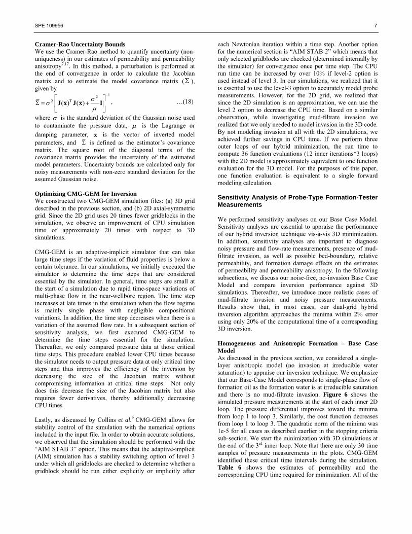
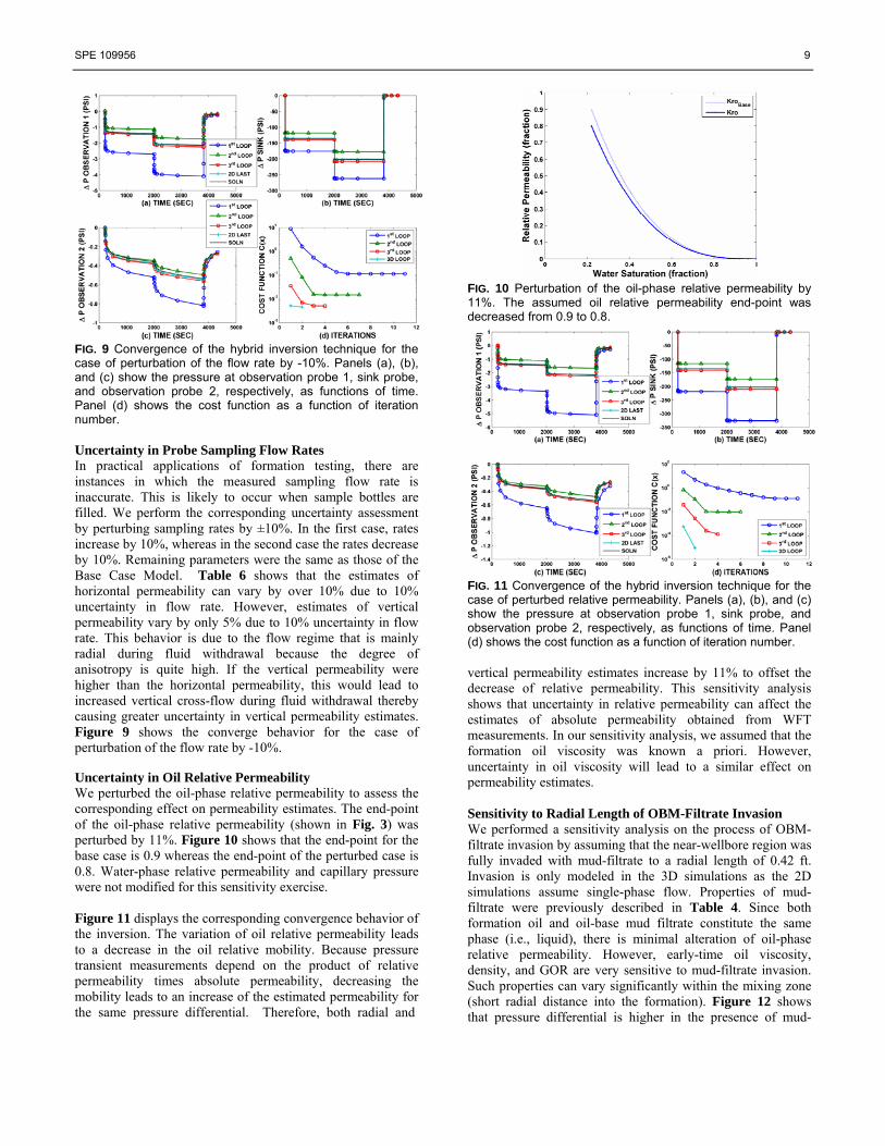
FIG. 9 Convergence of the hybrid inversion technique for the case of perturbation of the flow rate by -10%. Panels (a), (b), and (c) show the pressure at observation probe 1, sink probe, and observation probe 2, respectively, as functions of time. Panel (d) shows the cost function as a function of iteration number. Uncertainty in Probe Sampling Flow Rates In practical applications of formation testing, there are instances in which the measured sampling flow rate is inaccurate. This is likely to occur when sample bottles are filled. We perform the corresponding uncertainty assessment by perturbing sampling rates by ±10%. In the first case, rates increase by 10%, whereas in the second case the rates decrease by 10%. Remaining parameters were the same as those of the Base Case Model. Table 6 shows that the estimates of horizontal permeability can vary by over 10% due to 10% uncertainty in flow rate. However, estimates of vertical permeability vary by only 5% due to 10% uncertainty in flow rate. This behavior is due to the flow regime that is mainly radial during fluid withdrawal because the degree of anisotropy is quite high. If the vertical permeability were higher than the horizontal permeability, this would lead to increased vertical cross-flow during fluid withdrawal thereby causing greater uncertainty in vertical permeability estimates. Figure 9 shows the converge behavior for the case of perturbation of the flow rate by -10%. Uncertainty in Oil Relative Permeability We perturbed the oil-phase relative permeability to assess the corresponding effect on permeability estimates. The end-point of the oil-phase relative permeability (shown in Fig. 3) was perturbed by 11%. Figure 10 shows that the end-point for the base case is 0.9 whereas the end-point of the perturbed case is 0.8. Water-phase relative permeability and capillary pressure were not modified for this sensitivity exercise. Figure 11 displays the corresponding convergence behavior of the inversion. The variation of oil relative permeability leads to a decrease in the oil relative mobility. Because pressure transient measurements depend on the product of relative permeability times absolute permeability, decreasing the mobility leads to an increase of the estimated permeability for the same pressure differential. Therefore, both radial and

FIG. 10 Perturbation of the oil-phase relative permeability by 11%. The assumed oil relative permeability end-point was decreased from 0.9 to 0.8.

FIG. 11 Convergence of the hybrid inversion technique for the case of perturbed relative permeability. Panels (a), (b), and (c) show the pressure at observation probe 1, sink probe, and observation probe 2, respectively, as functions of time. Panel (d) shows the cost function as a function of iteration number. vertical permeability estimates increase by 11% to offset the decrease of relative permeability. This sensitivity analysis shows that uncertainty in relative permeability can affect the estimates of absolute permeability obtained from WFT measurements. In our sensitivity analysis, we assumed that the formation oil viscosity was known a priori. However, uncertainty in oil viscosity will lead to a similar effect on permeability estimates. Sensitivity to Radial Length of OBM-Filtrate Invasion We performed a sensitivity analysis on the process of OBM-filtrate invasion by assuming that the near-wellbore region was fully invaded with mud-filtrate to a radial length of 0.42 ft. Invasion is only modeled in the 3D simulations as the 2D simulations assume single-phase flow. Properties of mud-filtrate were previously described in Table 4. Since both formation oil and oil-base mud filtrate constitute the same phase (i.e., liquid), there is minimal alteration of oil-phase relative permeability. However, early-time oil viscosity, density, and GOR are very sensitive to mud-filtrate invasion. Such properties can vary significantly within the mixing zone (short radial distance into the formation). Figure 12 shows that pressure differential is higher in the presence of mud-

10 SPE 109956

filtrate invasion. The change of viscosity modifies the phase mobility with radial distance and, in turn, this affects early-time pressure differentials. At late times, when the near-probe region is cleaned from oil-base mud filtrate, sand-face pressure curves converge because of negligible variation of phase mobility due to low compositional contrasts. We note that time intervals of pressure measurements increased to 122 in panels (a), (b), and (c) as the flow regime becomes more dynamic in the presence of invasion thereby causing the simulator to take smaller time steps. Figure 13 compares the GOR of our Base Case Model for the present sensitivity analysis. The curvature of the GOR plot is very sensitive to the radial length of invasion and can be used to determine sample quality from WFT measurements. We note that, even after one hour of fluid pumpout, the GOR for the invasion case increases to 2057 SCF/STB whereas the Base Case exhibits a constant GOR equal to 2193 SCF/STB. Therefore, even a small fraction of mud-filtrate components present in the fluid stream at late times can substantially impact the GOR measurements and hence the sample quality. Table 6 shows that CPU time for the 3D simulation increases drastically when mud-filtrate invasion is taken into consideration. Each function evaluation of the 3D simulation takes approximately 740 sec. The 3D minimization after inner 2D loops takes 10891 sec of CPU time and decreases the permeability uncertainty by 1.3% vis-à-vis the hybrid minimization. In this instance, we could have achieved further savings of CPU time by stopping the inversion at the end of the 3rd loop or by adding a 4th loop of 2D minimization to prevent the use of a 3D minimization. Even without considering invasion in the 2D simulation, we were able to achieve inversion results within 1.3% of the corresponding results obtained with 3D inversion. This behavior indicates that our inversion technique can be easily extended to single-phase analytical solutions or commercial pressure transient software as an alternative to using the 2D simulation grid.

FIG. 12 Convergence of the hybrid inversion technique with presence of mud-filtrate invasion. Note that the pressure differential in the sink probe at early times is much higher than for the Base Case Model. Panels (a), (b), and (c) show the pressure at observation probe 1, sink probe, and observation probe 2, respectively, as functions of time. Panel (d) shows the cost function as a function of iteration number.

FIG. 13 Comparison of GOR for the Base Case Model and the case with 0.42 ft radial length of mud-filtrate invasion. The GOR for the Base Case is constant at 2193 SCF/STB because of the absence of invasion. Uncertainty in the Radial Length of OBM-filtrate Invasion We now consider the hypothetical case in which the inversion is performed without including transient GOR measurements (or, equivalently, by neglecting mud-filtrate invasion effects). To that end, we make use of pressure transient measurements previously simulated for the case of a radial length of invasion of 0.42 ft. Table 6 shows that unaccounted mud-filtrate invasion effects in the near-wellbore region cause significant errors in the permeability estimates. Both horizontal and vertical permeability estimates decrease due to the high-pressure differential. We observe that cost function is excessively large, even after the third minimization loop despite the fact that there is no Gaussian noise present in the measurements. Formation Damage due to Invasion There are instances in which the near-wellbore permeability decreases locally due to dynamic drilling conditions that cause solid particles to invade the formation along with mud-filtrate. To appraise such a deleterious condition on the inversion of pressure transient measurements, we performed a sensitivity analysis in which we assumed a horizontal permeability of 100 mD at 0.42 feet radially away from the wellbore and 200 mD elsewhere. Vertical permeability was assumed equal to 0.335 times the value of horizontal permeability. Inversion results show that it is difficult to obtain reliable estimates of permeability radially away into the formation in the presence of unaccounted invasion and formation damage. In this case, both the 3D minimization and the hybrid minimization were unable to approach the minimum of the cost function. Layered and Anisotropic Formation We assume a three-layer formation model with non-uniform layer thickness of 17 ft, 4 ft, and 21.75 ft from top to bottom of the formation. Observation probes are located at the center of the top two layers. Radial permeability of the layers are 200 mD, 150 mD, and 75 mD from top to bottom, respectively. Anisotropy ratio is assumed 0.335 and porosity is 0.18 for all the layers. Relative permeability and capillary pressure curves were assumed the same for all layers (shown in Fig. 3). Figure 14 displays the convergence behavior of the multi-layered case. Table 7 describes the values of permeability

SPE 109956 11

estimated from inversion. Results from this exercise indicate that our hybrid inversion technique is reliable to estimate the permeability values included in a multi-layer system.

TABLE 6: Summary of sensitivity analyses performed for the single-layer formation model. Permeability units are in mD and CPU time is in sec. CPU time for 2D loops include the time required for one 3D function evaluation. Sensitivity Parameter Loop 1 Loop 2 Loop 3 3D

minimization Base Case Model

kH=250.7 kV=60.12

kH=190.5 kV=65.79

kH=201.1 kV=66.84

kH=200 kV=67

Cost function 0.12445 0.01083 1.02e-4 6.8e-6 Funt. Evals. 14 9 7 5 CPU time 445 380 355 1443 Base Case Model (3D ONLY)

- - - kH=200 kV=67

Cost function - - - 8.1e-7 Funt. Evals. - - - 12 CPU time - - - 3113

Base Case Model (5% Noise)

kH=256.3 ±1.35 kV=56.97 ±1.17

kH=184.3 ±0.27 kV=63.12 ±0.025

kH=199.0 ±0.03 kV=64.28 ±0.03

kH=197.6 ±0.001 kV=62.14 ±0.001

Cost function 3.31329 3.19986 3.20719 3.20592 Funt. Evals. 13 13 6 5 CPU time 427 426 339 1436 Flow rate +10%

kH=283.3 kV=63.00

kH=209.8 kV=68.8

kH=223.6 kV=70.05

kH=221.7 kV=70.41

Cost function 0.13967 0.01463 0.00418 0.00419 Funt. Evals. 14 17 8 8 CPU time 459 479 366 2167 Flow rate -10%

kH=217.9 kV=58.18

kH=171.6 kV=62.07

kH=179.8 kV=62.93

kH=178.6 kV=63.5

Cost function 0.11531 0.01505 0.00511 0.00465 Funt. Evals. 14 10 7 5 CPU time 441 412 355 1452 Relative Permeability

kH=293.2 kV=66.04

kH=214.8 kV=74.19

kH=226.4 kV=75.37

kH=225.2 kV=75.47

Cost function 0.13239 0.00978 1.3e-4 9.4e-6 Funt. Evals. 14 9 7 5 CPU time 439 376 352 1447 OBM-filtrate Invasion

kH=272.2 kV=75.67

kH=188.9 kV=65.01

kH=202.6 kV=67.18

kH=200.0 kV=67.01

Cost function 1.30456 0.05141 0.00254 7.9e-6 Funt. Evals. 13 13 13 14 CPU time 1127 1202 1111 10891 Invasion Uncertainty

kH=231.5 kV=34.62

kH=166.6 kV=35.74

kH=173.8 kV=36.04

kH=172.8 kV=39.84

Cost function 12.7397 13.8576 13.4828 13.4801 Funt. Evals. 13 15 15 14 CPU time 930 987 990 8349 Formation Damage

k1=110.9 k2=166.4

k1=110.9 k2=166.4

k1=110.9 k2=166.4

k1=110.9 k2=166.4

Cost function 2.08271 1.67854 1.67854 1.67854 Funt. Evals. 13 15 15 15 CPU time 1102 1331 1332 14307

Effect of 5% Noise in Pressure Measurements Similar to the case of adding noise for the Base Case Model, we added 5% Gaussian noise to the sink-probe pressure measurements and 2.5% noise to the observation-probe pressure measurements simulated for the multi-layer formation. Table 7 indicates that the estimated layer permeabilities are marginally affected by presence of noise in the transient pressure measurements.

FIG. 14 Convergence of the hybrid inversion technique for the three-layer formation model. Pressure differential at the sink probe is relatively high due to the reduced horizontal permeability of 75 mD. Panels (a), (b), and (c) show the pressure at observation probe 1, sink probe, and observation probe 2, respectively, as functions of time. Panel (d) shows the cost function as a function of iteration number.

FIG. 15 Convergence of the hybrid inversion technique for the case of incorrect single-layer assumption for the three-layer formation model and noisy measurements. Panels (a), (b), and (c) show the pressure at observation probe 1, sink probe, and observation probe 2, respectively, as functions of time. Panel (d) shows the cost function as a function of iteration number.

12 SPE 109956

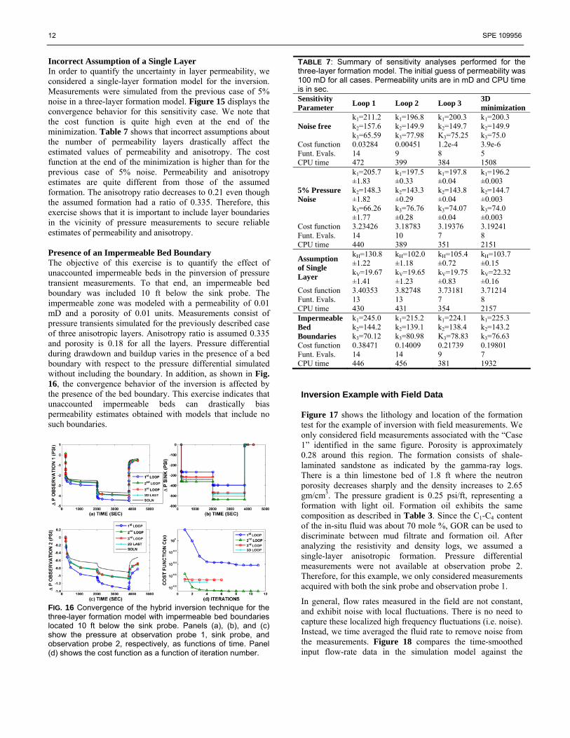
Incorrect Assumption of a Single Layer In order to quantify the uncertainty in layer permeability, we considered a single-layer formation model for the inversion. Measurements were simulated from the previous case of 5% noise in a three-layer formation model. Figure 15 displays the convergence behavior for this sensitivity case. We note that the cost function is quite high even at the end of the minimization. Table 7 shows that incorrect assumptions about the number of permeability layers drastically affect the estimated values of permeability and anisotropy. The cost function at the end of the minimization is higher than for the previous case of 5% noise. Permeability and anisotropy estimates are quite different from those of the assumed formation. The anisotropy ratio decreases to 0.21 even though the assumed formation had a ratio of 0.335. Therefore, this exercise shows that it is important to include layer boundaries in the vicinity of pressure measurements to secure reliable estimates of permeability and anisotropy. Presence of an Impermeable Bed Boundary The objective of this exercise is to quantify the effect of unaccounted impermeable beds in the pinversion of pressure transient measurements. To that end, an impermeable bed boundary was included 10 ft below the sink probe. The impermeable zone was modeled with a permeability of 0.01 mD and a porosity of 0.01 units. Measurements consist of pressure transients simulated for the previously described case of three anisotropic layers. Anisotropy ratio is assumed 0.335 and porosity is 0.18 for all the layers. Pressure differential during drawdown and buildup varies in the presence of a bed boundary with respect to the pressure differential simulated without including the boundary. In addition, as shown in Fig. 16, the convergence behavior of the inversion is affected by the presence of the bed boundary. This exercise indicates that unaccounted impermeable beds can drastically bias permeability estimates obtained with models that include no such boundaries.

FIG. 16 Convergence of the hybrid inversion technique for the three-layer formation model with impermeable bed boundaries located 10 ft below the sink probe. Panels (a), (b), and (c) show the pressure at observation probe 1, sink probe, and observation probe 2, respectively, as functions of time. Panel (d) shows the cost function as a function of iteration number.

TABLE 7: Summary of sensitivity analyses performed for the three-layer formation model. The initial guess of permeability was 100 mD for all cases. Permeability units are in mD and CPU time is in sec. Sensitivity Parameter Loop 1 Loop 2 Loop 3 3D

minimization

Noise free k1=211.2 k2=157.6 k3=65.59

k1=196.8 k2=149.9 k3=77.98

k1=200.3 k2=149.7 K3=75.25

k1=200.3 k2=149.9 k3=75.0

Cost function 0.03284 0.00451 1.2e-4 3.9e-6 Funt. Evals. 14 9 8 5 CPU time 472 399 384 1508

5% Pressure Noise

k1=205.7 ±1.83 k2=148.3 ±1.82 k3=66.26 ±1.77

k1=197.5 ±0.33 k2=143.3 ±0.29 k3=76.76 ±0.28

k1=197.8 ±0.04 k2=143.8 ±0.04 k3=74.07 ±0.04

k1=196.2 ±0.003 k2=144.7 ±0.003 k3=74.0 ±0.003

Cost function 3.23426 3.18783 3.19376 3.19241 Funt. Evals. 14 10 7 8 CPU time 440 389 351 2151

Assumption of Single Layer

kH=130.8 ±1.22 kV=19.67 ±1.41

kH=102.0 ±1.18 kV=19.65 ±1.23

kH=105.4 ±0.72 kV=19.75 ±0.83

kH=103.7 ±0.15 kV=22.32 ±0.16

Cost function 3.40353 3.82748 3.73181 3.71214 Funt. Evals. 13 13 7 8 CPU time 430 431 354 2157 Impermeable Bed Boundaries

k1=245.0 k2=144.2 k3=70.12

k1=215.2 k2=139.1 k3=80.98

k1=224.1 k2=138.4 K3=78.83

k1=225.3 k2=143.2 k3=76.63

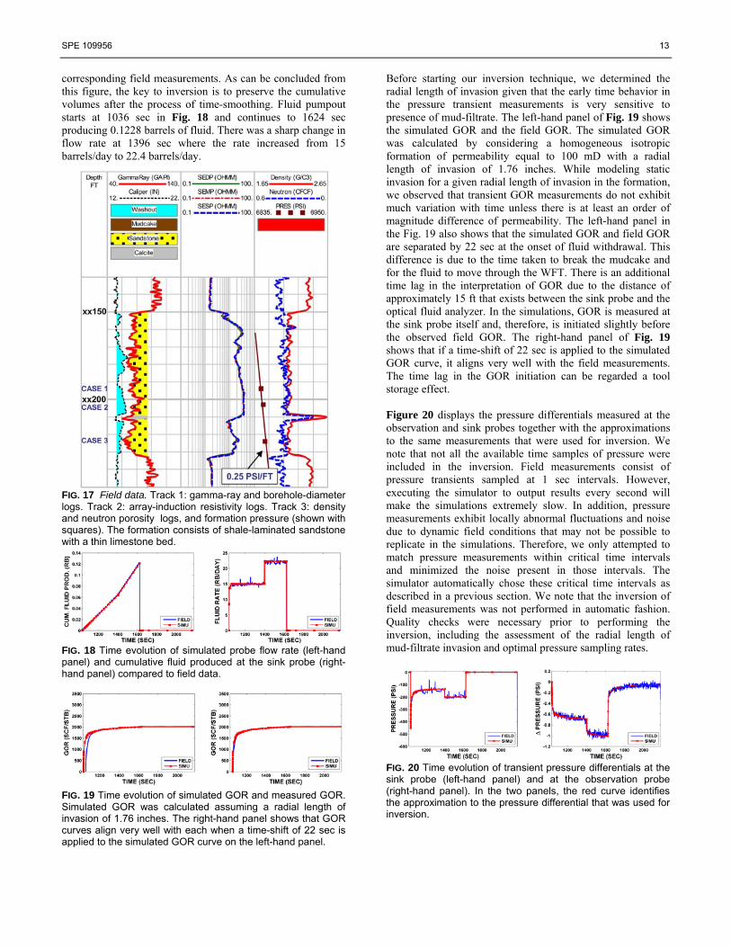
Cost function 0.38471 0.14009 0.21739 0.19801 Funt. Evals. 14 14 9 7 CPU time 446 456 381 1932 Inversion Example with Field Data Figure 17 shows the lithology and location of the formation test for the example of inversion with field measurements. We only considered field measurements associated with the “Case 1” identified in the same figure. Porosity is approximately 0.28 around this region. The formation consists of shale-laminated sandstone as indicated by the gamma-ray logs. There is a thin limestone bed of 1.8 ft where the neutron porosity decreases sharply and the density increases to 2.65 gm/cm3. The pressure gradient is 0.25 psi/ft, representing a formation with light oil. Formation oil exhibits the same composition as described in Table 3. Since the C1-C4 content of the in-situ fluid was about 70 mole %, GOR can be used to discriminate between mud filtrate and formation oil. After analyzing the resistivity and density logs, we assumed a single-layer anisotropic formation. Pressure differential measurements were not available at observation probe 2. Therefore, for this example, we only considered measurements acquired with both the sink probe and observation probe 1.

In general, flow rates measured in the field are not constant, and exhibit noise with local fluctuations. There is no need to capture these localized high frequency fluctuations (i.e. noise). Instead, we time averaged the fluid rate to remove noise from the measurements. Figure 18 compares the time-smoothed input flow-rate data in the simulation model against the

SPE 109956 13

corresponding field measurements. As can be concluded from this figure, the key to inversion is to preserve the cumulative volumes after the process of time-smoothing. Fluid pumpout starts at 1036 sec in Fig. 18 and continues to 1624 sec producing 0.1228 barrels of fluid. There was a sharp change in flow rate at 1396 sec where the rate increased from 15 barrels/day to 22.4 barrels/day.

FIG. 17 Field data. Track 1: gamma-ray and borehole-diameter logs. Track 2: array-induction resistivity logs. Track 3: density and neutron porosity logs, and formation pressure (shown with squares). The formation consists of shale-laminated sandstone with a thin limestone bed.

FIG. 18 Time evolution of simulated probe flow rate (left-hand panel) and cumulative fluid produced at the sink probe (right-hand panel) compared to field data.

FIG. 19 Time evolution of simulated GOR and measured GOR. Simulated GOR was calculated assuming a radial length of invasion of 1.76 inches. The right-hand panel shows that GOR curves align very well with each when a time-shift of 22 sec is applied to the simulated GOR curve on the left-hand panel.

Before starting our inversion technique, we determined the radial length of invasion given that the early time behavior in the pressure transient measurements is very sensitive to presence of mud-filtrate. The left-hand panel of Fig. 19 shows the simulated GOR and the field GOR. The simulated GOR was calculated by considering a homogeneous isotropic formation of permeability equal to 100 mD with a radial length of invasion of 1.76 inches. While modeling static invasion for a given radial length of invasion in the formation, we observed that transient GOR measurements do not exhibit much variation with time unless there is at least an order of magnitude difference of permeability. The left-hand panel in the Fig. 19 also shows that the simulated GOR and field GOR are separated by 22 sec at the onset of fluid withdrawal. This difference is due to the time taken to break the mudcake and for the fluid to move through the WFT. There is an additional time lag in the interpretation of GOR due to the distance of approximately 15 ft that exists between the sink probe and the optical fluid analyzer. In the simulations, GOR is measured at the sink probe itself and, therefore, is initiated slightly before the observed field GOR. The right-hand panel of Fig. 19 shows that if a time-shift of 22 sec is applied to the simulated GOR curve, it aligns very well with the field measurements. The time lag in the GOR initiation can be regarded a tool storage effect. Figure 20 displays the pressure differentials measured at the observation and sink probes together with the approximations to the same measurements that were used for inversion. We note that not all the available time samples of pressure were included in the inversion. Field measurements consist of pressure transients sampled at 1 sec intervals. However, executing the simulator to output results every second will make the simulations extremely slow. In addition, pressure measurements exhibit locally abnormal fluctuations and noise due to dynamic field conditions that may not be possible to replicate in the simulations. Therefore, we only attempted to match pressure measurements within critical time intervals and minimized the noise present in those intervals. The simulator automatically chose these critical time intervals as described in a previous section. We note that the inversion of field measurements was not performed in automatic fashion. Quality checks were necessary prior to performing the inversion, including the assessment of the radial length of mud-filtrate invasion and optimal pressure sampling rates.

FIG. 20 Time evolution of transient pressure differentials at the sink probe (left-hand panel) and at the observation probe (right-hand panel). In the two panels, the red curve identifies the approximation to the pressure differential that was used for inversion.

14 SPE 109956

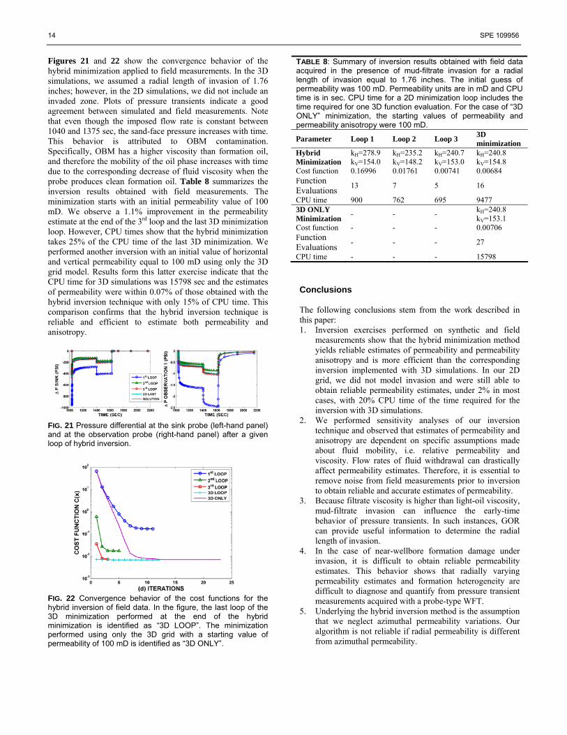
Figures 21 and 22 show the convergence behavior of the hybrid minimization applied to field measurements. In the 3D simulations, we assumed a radial length of invasion of 1.76 inches; however, in the 2D simulations, we did not include an invaded zone. Plots of pressure transients indicate a good agreement between simulated and field measurements. Note that even though the imposed flow rate is constant between 1040 and 1375 sec, the sand-face pressure increases with time. This behavior is attributed to OBM contamination. Specifically, OBM has a higher viscosity than formation oil, and therefore the mobility of the oil phase increases with time due to the corresponding decrease of fluid viscosity when the probe produces clean formation oil. Table 8 summarizes the inversion results obtained with field measurements. The minimization starts with an initial permeability value of 100 mD. We observe a 1.1% improvement in the permeability estimate at the end of the 3rd loop and the last 3D minimization loop. However, CPU times show that the hybrid minimization takes 25% of the CPU time of the last 3D minimization. We performed another inversion with an initial value of horizontal and vertical permeability equal to 100 mD using only the 3D grid model. Results form this latter exercise indicate that the CPU time for 3D simulations was 15798 sec and the estimates of permeability were within 0.07% of those obtained with the hybrid inversion technique with only 15% of CPU time. This comparison confirms that the hybrid inversion technique is reliable and efficient to estimate both permeability and anisotropy.

FIG. 21 Pressure differential at the sink probe (left-hand panel) and at the observation probe (right-hand panel) after a given loop of hybrid inversion.

FIG. 22 Convergence behavior of the cost functions for the hybrid inversion of field data. In the figure, the last loop of the 3D minimization performed at the end of the hybrid minimization is identified as “3D LOOP”. The minimization performed using only the 3D grid with a starting value of permeability of 100 mD is identified as “3D ONLY”.

TABLE 8: Summary of inversion results obtained with field data acquired in the presence of mud-filtrate invasion for a radial length of invasion equal to 1.76 inches. The initial guess of permeability was 100 mD. Permeability units are in mD and CPU time is in sec. CPU time for a 2D minimization loop includes the time required for one 3D function evaluation. For the case of “3D ONLY” minimization, the starting values of permeability and permeability anisotropy were 100 mD.

Parameter Loop 1 Loop 2 Loop 3 3D minimization

Hybrid Minimization

kH=278.9 kV=154.0

kH=235.2 kV=148.2

kH=240.7 kV=153.0

kH=240.8 kV=154.8

Cost function 0.16996 0.01761 0.00741 0.00684 Function Evaluations

13 7 5 16

CPU time 900 762 695 9477 3D ONLY Minimization - - - kH=240.8

kV=153.1 Cost function - - - 0.00706 Function Evaluations

- - - 27

CPU time - - - 15798

Conclusions The following conclusions stem from the work described in this paper: 1. Inversion exercises performed on synthetic and field

measurements show that the hybrid minimization method yields reliable estimates of permeability and permeability anisotropy and is more efficient than the corresponding inversion implemented with 3D simulations. In our 2D grid, we did not model invasion and were still able to obtain reliable permeability estimates, under 2% in most cases, with 20% CPU time of the time required for the inversion with 3D simulations.

2. We performed sensitivity analyses of our inversion technique and observed that estimates of permeability and anisotropy are dependent on specific assumptions made about fluid mobility, i.e. relative permeability and viscosity. Flow rates of fluid withdrawal can drastically affect permeability estimates. Therefore, it is essential to remove noise from field measurements prior to inversion to obtain reliable and accurate estimates of permeability.

3. Because filtrate viscosity is higher than light-oil viscosity, mud-filtrate invasion can influence the early-time behavior of pressure transients. In such instances, GOR can provide useful information to determine the radial length of invasion.

4. In the case of near-wellbore formation damage under invasion, it is difficult to obtain reliable permeability estimates. This behavior shows that radially varying permeability estimates and formation heterogeneity are difficult to diagnose and quantify from pressure transient measurements acquired with a probe-type WFT.

5. Underlying the hybrid inversion method is the assumption that we neglect azimuthal permeability variations. Our algorithm is not reliable if radial permeability is different from azimuthal permeability.

SPE 109956 15

6. We evaluated the hybrid inversion method on field measurements and observed that the estimated values if permeability were within 0.07% of those obtained with the corresponding 3D inversion but within 15% of the CPU time. However, quality checks are necessary to reduce deleterious noise from pressure measurements prior to performing the inversion and to determine the associated flow rate of fluid withdrawal and radial length of invasion. We found that early-time pressure measurements could provide useful information to quantify fluid and formation properties.

Acknowledgements We are thankful to Mr. Bob Brugman (CMG) for his guidance in implementing simulation cases with CMG-GEM. The work reported in this paper was funded by the University of Texas at Austin’s Research Consortium on Formation Evaluation, jointly sponsored by Anadarko Petroleum Corporation, Aramco, Baker Atlas, British Gas, BHP Billiton, BP, ChevronTexaco, ConocoPhillips, ENI E&P, ExxonMobil, Halliburton, Hydro, Instituto Mexicano del Petróleo, Marathon Oil Corporation, Occidental Petroleum, Petrobras, Schlumberger, Shell International E&P, Statoil, Total, and Weatherford. References 1. Malik, M., Torres-Verdín, C., and Sepehrnoori, K.:

“Axially symmetric compositional simulation of formation tester measurements,” Journal of Petroleum Science and Engineering, In press, 2007.

2. Alpak, F.O., Elshahawi, H., and Hashem, M.: “Compositional modeling of oil-base mud-filtrate cleanup during wireline formation tester sampling,” paper SPE 100393, presented at the SPE Annual Technical Conference and Exhibition, San Antonio, Texas, September 24-27, 2006.

3. Zeybek, M., Ramakrishnan, T.S., Al-Otaibi, S.S., Salamy, S.P., and Kuchuk, F.J.: “Estimating multiphase flow properties using pressure and flowline water-cut from dual packer formation tester interval tests and openhole array resistivity measurements,” paper SPE 71568, presented at the SPE Annual Technical Conference and Exhibition, New Orleans, Louisiana, September 30-October 3, 2001.

4. Gok, I.M., Onur, M., Hegeman, P.S., and Kuchuk, F.J.: “Effect of an invaded zone on pressure-transient data from multiprobe and packer-probe wireline formation testers,” SPEREE, v. 9, no. 1, pp. 39-49, February, 2006.

5. Torres-Verdín, C., Druskin, V.L., Fang, S., Knizhnerman, L.A., and Malinverno, A.: “A dual-grid inversion technique with applications to the interpretation of dc resistivity data,” Geophysics, v. 65, no. 6, pp. 1733-1745, 2000.

6. McCalmont, S., Onu, C., Wu, J., Kiome, P., Sheng, J.J., Adegbola, F., Rajasingham, R., and Lee, J.: “Predicting pump-out volume and time based on sensitivity analysis for an efficient sampling operation: prejob modeling through a near-wellbore simulator,” paper SPE 95885, presented at the SPE Annual Technical Conference and Exhibition, Dallas, Texas, October 9-12, 2005.

7. Angeles, R., Lee, H.J., Alpak, F.O., Torres-Verdín, C., and Sheng, J.: “Efficient and accurate estimation of permeability and permeability anisotropy from straddle-packer formation tester measurements using the physics of two-phase immiscible flow and invasion,” paper SPE 95897, presented at the SPE Annual Technical Conference and Exhibition, Dallas, Texas, October 9-12, 2005.

8. Wu, J., Torres-Verdín, C., Proett, M.A., Sepehrnoori, K., and Belanger, D.: “Inversion of multi-phase petrophysical properties using pumpout sampling data acquired with a wireline formation tester,” paper SPE 77345, presented at the SPE Annual Technical Conference and Exhibition, San Antonio, Texas, September 29-October 2, 2002.

9. Collins, D.A., Nghiem, L.X., Li, Y.K., and Grabenstetter, J.E.: “An efficient approach to adaptive-implicit compositional simulation with an equation of state,” SPERE, v. 4, no. 6, pp. 259-264, May, 1992.

10. Peng, D.Y. and Robinson, D. B.: “A new two-constant equation of state,” Industrial and Engineering Chemistry Fundamentals, v. 15, no. 59, 1976.

11. Lohrenz, J., Bray, B. G., and Clark, C. R.: “Calculating viscosity of reservoir fluids from their compositions,” Journal of Petroleum Technology, SPE 915, pp. 1171-1176, October 1964.

12. Brooks, R.H. and Corey, A.T.: “Hydraulic properties of porous media,” Hydrology Paper 3, Colorado State University, Fort Collins, Colorado, 1964.

13. Levenberg, K.: “A method for the solution of certain problems in least squares,” Quart. Appl. Math., v. 2, pp. 164–168, 1944.

14. Marquardt, D.: “An algorithm for least squares estimation on nonlinear parameters,” SIAM J. Appl. Math., v. 11, pp. 431–441, 1963.

15. Broyden, C.G.: “A class of methods for solving nonlinear simultaneous equations,” Maths Comp., v. 19, pp. 577–593, 1965.

16. Madsen, K., Nielsen, H.B., and Tingleff, O.: “Methods for non-linear least squares problems,” 2nd Edition IMM, DTU 2004.

17. Habashy, T.M. and Abubakar, A.: “A general framework for constraint minimization for the inversion of electromagnetic measurements,” Progress in Electromagnetic Research, v. 46, pp. 265-312, 2004.