Embed Size (px)
Citation preview

1/20
Accelerating minimizations in ensemble variational assimilation
G. Desroziers, L. BerreMétéo-France/CNRS (CNRM/GAME)
2/20
Outline
1. Ensemble Variational assimilation
2. Accelerating minimizations
3. Conclusion and future work

3/20
Outline
1. Ensemble Variational assimilation
2. Accelerating minimizations
3. Conclusion and future work
4/20
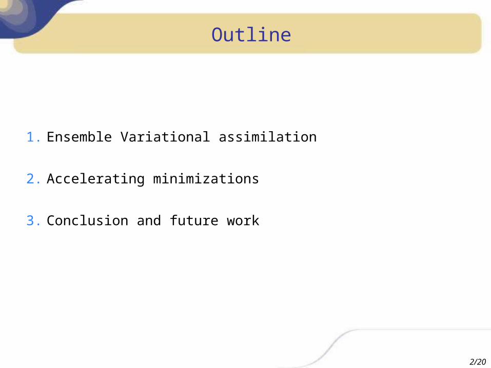
Simulation of analysis errors : «hybrid EnKF/Var» or «consistent ensemble 4D-Var»?
A consistent 4D-Var approach can be used in both ensemble and deterministic components :
Simple to implement (perturbed Var ~ unperturbed Var).
A full-rank hybrid B is consistently used in the 2 parts.
Non-linear aspects of 4D-Var can be represented (outer loop).
5/20
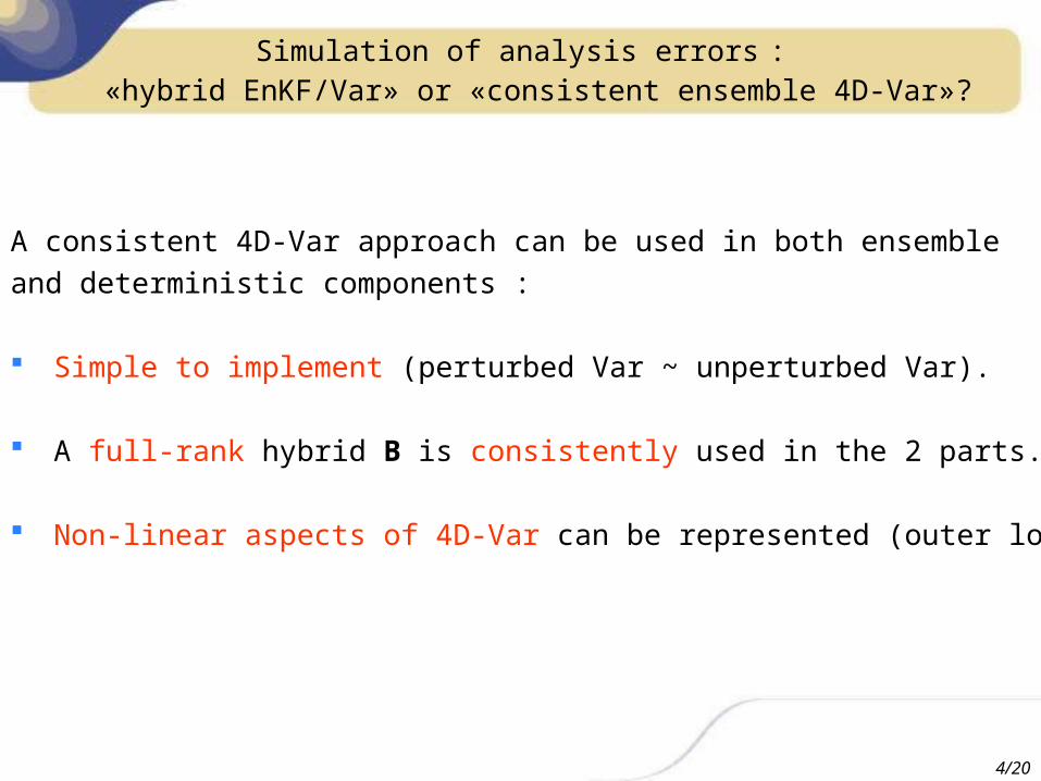
The operational Météo-France ensemble Var assimilation
Six perturbed global members, T399 L70 (50 km / 10 km), with global 4D-Var Arpege.
Spatial filtering of error variances, to further increase the sample size and robustness.
Inflation of ensemble B / model error contributions,soon replaced by inflation of perturbations.
6/20
Applications of the EnDA system at Météo-France
Flow-dependent background error variances in 4D-Var.
Flow-dependent background error correlations experimented
using wavelet filtering properties (Varella et al 2011 a,b) .
Initialisation of Météo-France ensemble prediction by EnDA.
Diagnostics on analysis consistency and observation impact
(Desroziers et al 2009) .
7/20
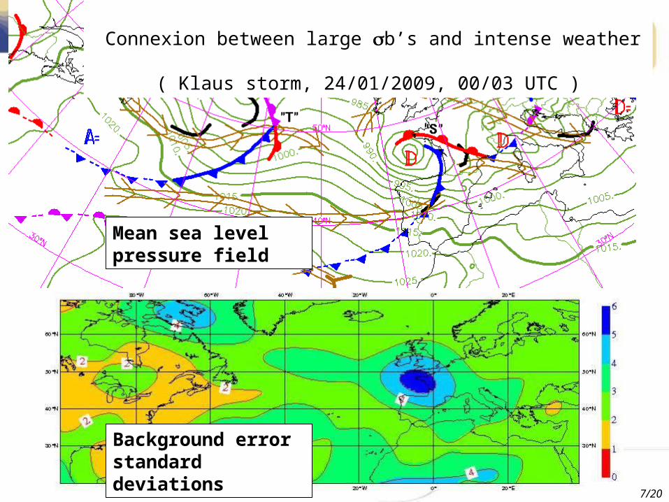
Background error standard deviations
Connexion between large b’s and intense weather ( Klaus storm, 24/01/2009, 00/03 UTC )
Mean sea level pressure field
8/20
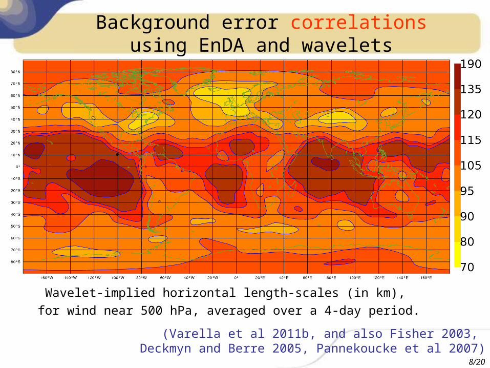
Background error correlationsusing EnDA and wavelets
Wavelet-implied horizontal length-scales (in km), for wind near 500 hPa, averaged over a 4-day period.
(Varella et al 2011b, and also Fisher 2003, Deckmyn and Berre 2005, Pannekoucke et al 2007)
9/20
Outline
1. Ensemble Variational assimilation
2. Accelerating minimizations
3. Conclusion and future work
10/20
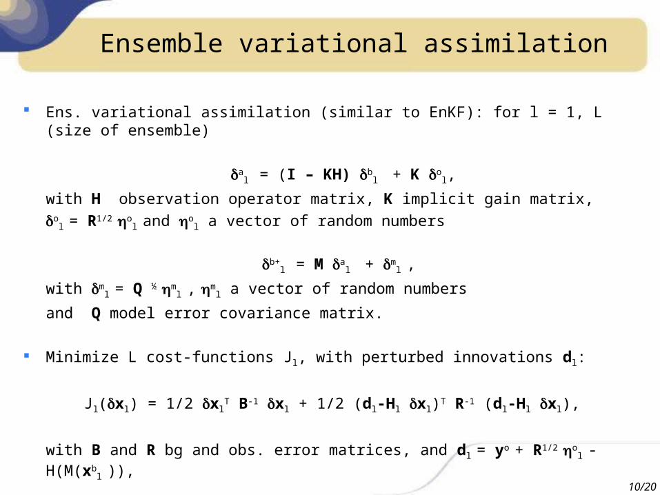
Ensemble variational assimilation
Ens. variational assimilation (similar to EnKF): for l = 1, L (size of ensemble)
a
l = (I – KH) b
l + K o
l, with H observation operator matrix, K implicit gain matrix, o
l = R1/2 ol and o
l a vector of random numbers
b+l = M a
l + m
l ,
with ml = Q ½ m
l , ml a vector of random numbers
and Q model error covariance matrix.
Minimize L cost-functions Jl, with perturbed innovations dl:
Jl(xl) = 1/2 xlT B-1 xl + 1/2 (dl-Hl xl)T R-1 (dl-Hl xl),
with B and R bg and obs. error matrices, and dl = yo + R1/2 ol - H(M(xb
l )),
xal = xb
l + xl and xbl+ = M( xa
l) + Q1/2 ml .
11/20
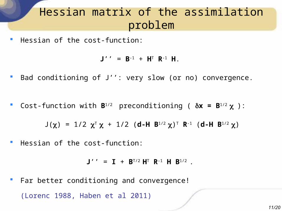
Hessian matrix of the assimilation problem
Hessian of the cost-function:
J’’ = B-1 + HT R-1 H.
Bad conditioning of J’’: very slow (or no) convergence.
Cost-function with B1/2 preconditioning ( x = B1/2 ):
J() = 1/2 T + 1/2 (d-H B1/2 )T R-1 (d-H B1/2 )
Hessian of the cost-function:
J’’ = I + BT/2 HT R-1 H B1/2 .
Far better conditioning and convergence!
(Lorenc 1988, Haben et al 2011)
12/20
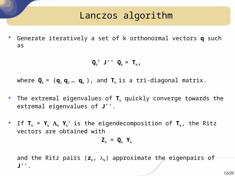
Lanczos algorithm
Generate iteratively a set of k orthonormal vectors q such as
QkT J’’ Qk = Tk,
where Qk = (q1 q2 … qk ), and Tk is a tri-diagonal matrix.
The extremal eigenvalues of Tk quickly converge towards the extremal eigenvalues of J’’.
If Tk = Yk k YkT is the eigendecomposition of Tk, the Ritz vectors are
obtained withZk = Qk Yk
and the Ritz pairs (zk, k) approximate the eigenpairs of J’’.
13/20
Lanczos algorithm / Conjugate gradient
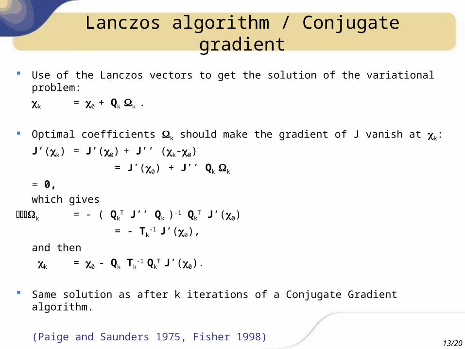
Use of the Lanczos vectors to get the solution of the variational problem:
k = 0 + Qk k .
Optimal coefficients k should make the gradient of J vanish at k:
J’(k) = J’(0) + J’’ (k-0)
= J’(0) + J’’ Qk k
= 0,which gives
k = - ( QkT J’’ Qk )-1 Qk
T J’(0)
= - Tk-1
J’(0),
and then k = 0 - Qk Tk
-1 Qk
T J’(0).
Same solution as after k iterations of a Conjugate Gradient algorithm.
(Paige and Saunders 1975, Fisher 1998)
14/20
Minimizations with
- unperturbed innovations d and - perturbed innovations dl have basically the same Hessians:
J’’(d) = I + BT/2 HT R-1 H B1/2 ,
J’’(dl) = I + BT/2 HlT R-1 Hl B1/2 ,
The solution obtained for the « unperturbed » problem
k = 0 - Qk ( QkT J’’ Qk )-1
QkT J’(0, d)
can be transposed to the « perturbed » minimization
k,l = 0 - Qk ( QkT J’’ Qk )-1
QkT J’(0, dl)
to improve its starting point.
Accelerating a « perturbed » minimization using « unperturbed » Lanczos vectors
15/20
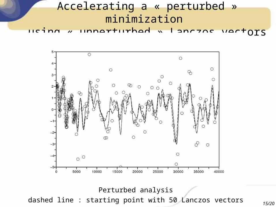
Accelerating a « perturbed » minimization using « unperturbed » Lanczos vectors
Perturbed analysisdashed line : starting point with 50 Lanczos vectors
16/20
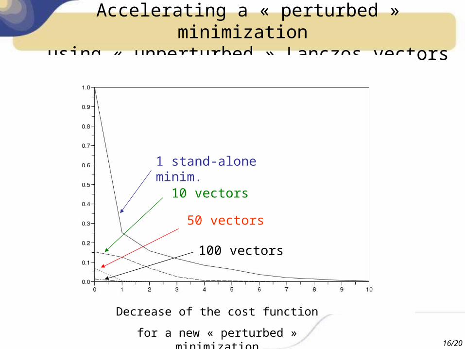
Accelerating a « perturbed » minimization using « unperturbed » Lanczos vectors
Decrease of the cost function
for a new « perturbed » minimization
1 stand-alone minim.
10 vectors
50 vectors
100 vectors
17/20
Accelerating minimizations using « perturbed » Lanczos vectors
If L perturbed minim. with k iterations have already been performed, then the starting point of a perturbed (or unperturbed) minimizationcan be written under the form
k = 0 + Qk,L k,L,
where k,L is a vector of k x L coefficients and
Qk,L = (q1,1 … qk,1 … q1,L … qk,L )
is a matrix containing the k x L Lanczos vectors.
Following the same approach as above, the solution can be expressed and computed:
k,L = 0 – Qk,L ( Qk,LT J’’ Qk,L )-1 Qk,L
T J’(0).
Matrix Qk,LT J’’ Qk,L is no longer tri-diagonal, but can be easily inverted.
18/20
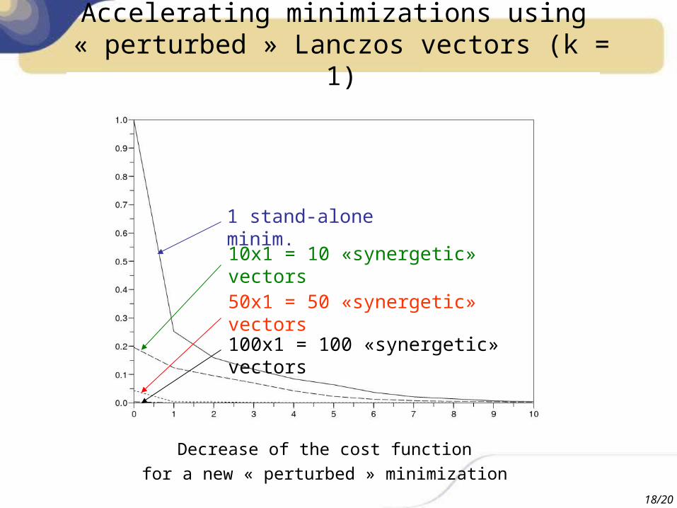
1 stand-alone minim.
10x1 = 10 «synergetic» vectors50x1 = 50 «synergetic» vectors
Decrease of the cost functionfor a new « perturbed » minimization
Accelerating minimizations using « perturbed » Lanczos vectors (k = 1)
100x1 = 100 «synergetic» vectors
19/20
Outline
1. Ensemble Variational assimilation
2. Accelerating minimizations
3. Conclusion and future work
20/20
Conclusion and future work
Ensemble Variational assimilation: error cycling can be simulated in a way consistent with 4D-Var.
Flow-dependent covariances can be estimated.
Positive impacts, in particular for intense/severe weather events, from both flow-dependent variances and correlations.
Accelerating minimizations seems possible(preliminary tests in the real size Ens. 4D-Var Arpege also encouraging).
Connection with Block Lanczos / CG algorithms (O’Leary 1980) .
Possible appl. in EnVar without TL/AD (Lorenc 2003, Buehner 2005) .