Spatiotemporal Composition of Pest Ant Species in the ... · (RIFA). Fourteen different species were identified from the one-year-old site. However, RIFA ... Mullins for always having

Spatiotemporal Composition of Pest

Ant Species in the Residential Environments

of Santa Isabel, Puerto Rico

Preston Hunter Brown

Thesis submitted to the Faculty of the

Virginia Polytechnic Institute and State University in partial fulfillment of the requirements for the degree of

Master of Science In

Entomology

Dini M. Miller (Committee Chair)

Carlyle C. Brewster

Richard D. Fell

April 3, 2009 Blacksburg, Virginia Tech

Keywords: Ants, Diversity, Puerto Rico, Succession

Copyright 2009, Preston H. Brown

Spatiotemporal Composition of Pest Ant Species in the Residential

Environments of Santa Isabel, Puerto Rico

Preston Hunter Brown

(ABSTRACT)

Few studies have evaluated the community dynamics of pest ant species in tropical urban

environments. Pest ant community dynamics were examined within three Puerto Rican housing

developments. Housing developments (one, four, and eight years old), representing different

stages of urban succession were sampled to determine which species were present and the

relative species abundance. Eight trips were made to Puerto Rico over a one-year period, and

more than 1,000 samples were collected during each trip. The ants collected in each sample

were counted and identified. A total of 25 different species were identified from the

developments, with the major pest species being big-headed, rover, and red imported fire ants

(RIFA). Fourteen different species were identified from the one-year-old site. However, RIFA

and rover ants were the most abundant, accounting for >75% of ants collected. In the four-year-

old site, 20 species were identified. However, three species (RIFA, big-headed, and destructive

trailing ants) were dominant, accounting for >75% of ants collected. Sampling data from the

eight-year-old site indicated that out of 21 species identified, four species were dominant (RIFA,

crazy, and two species of big-headed ants) and accounted for >75% of the ants collected. The

dominant species within each site were different, indicating that the pest ant community changed

during the stages of succession. However, these dominant species did not specifically impact the

distribution of other species within the same site. Spatial analysis indicated that the number of

species coexisting within a site increased as the age of the development increased.

iii

ACKNOWLEDGEMENTS

First and foremost, I would like to express my sincere gratitude to my advisor and friend,

Dr. Dini M. Miller. Dr. Miller has contributed a significant amount of time and energy into my

degree, and for that I am extremely grateful. All of my academic achievements are largely due

to her efforts and encouragement. She has pushed, and at times dragged, me to be the best I can

be, “...and that has made all the difference.”

I would also like to express my gratitude to the other members of my committee, Dr.

Carlyle C. Brewster and Dr. Richard D. Fell for their time and assistance during my studies at

Virginia Tech. They have both taught me so much.

I would also like to thank those individuals who contributed to my research project. Don

Bieman was instrumental in helping me to find my research sites and provided additional

assistance while I was in Puerto Rico. Alan Harms supplied me with weather data for my sites

and showed me around Santa Isabel. Roy Snelling and Juan Torres provided me with a copy of

their manuscript on the ants of Puerto Rico which was invaluable in identifying all 243,252 ants.

Additionally, Matthew Buffington and Mark Deyrup offered their taxonomic assistance with ant

identifications. Dr. Eric Smith of the Virginia Tech Department of Statistics contributed a great

amount of time and guidance with the statistical sections of my thesis.

I am extremely grateful to the members of the Dodson Urban Pest Management

Laboratory for their support and friendship: to Tim McCoy for all his technical assistance and

encouragement, David Moore for being stronger than he looks, Hamilton Allen for keeping it

real, and Marc Fisher for giving me possibly the best advice when I began my graduate degree

(treat it like a job and apply for everything!). A special thank you to Tamara Sutphin for the

hours and hours she spent helping me process my samples. I would still be counting ants without

her help.

I would like to thank the faculty, staff, and, students in the Virginia Tech Department of

Entomology for their assistance and support. Specifically I would like to thank Dr. Donald

Mullins for always having an encouraging word to say, and Dr. Loke Kok for his advice and

always having an open door. I also cannot thank Kathy Shelor, Sarah Kenley, and Robin

Williams enough for everything they have done for me over the last four years. These three

iv

amazing ladies have always been willing to help me with whatever I needed, and for that I am

grateful.

I would also like to express my gratitude to the W. B. Alwood Society, the Entomological

Society of America, the National Conference on Urban Entomology, Sigma Xi, the Virginia Pest

Management Association, as well as Dr. Clay Scherer of DuPont, and the fabulous Coron sisters,

Andrea and Kristin.

I would also like to thank all of the many people I have met along the way for their

friendship and support, specifically Lisa Burley, Tim Jordan, Susan Sherbak, Kim Daniloski, Jen

Dvorsky, Rob Tompkins, and Ryan McMahan.

Finally, I want to thank my parents, Paul and Betsy Brown, and my brother, Aaron

Brown, for their unconditional support, love, and constant encouragement. Truly, I am blessed.

v

DEDICATION

In loving memory of my grandparents, Mary Ruth Smith Orr, Lois Anne Peace Brown, and

Charles Raymond Brown, Jr.

vi

TABLE OF CONTENTS

Acknowledgements ................................................................................................................. iii

Dedication ................................................................................................................................... v

List of Figures ........................................................................................................................ viii

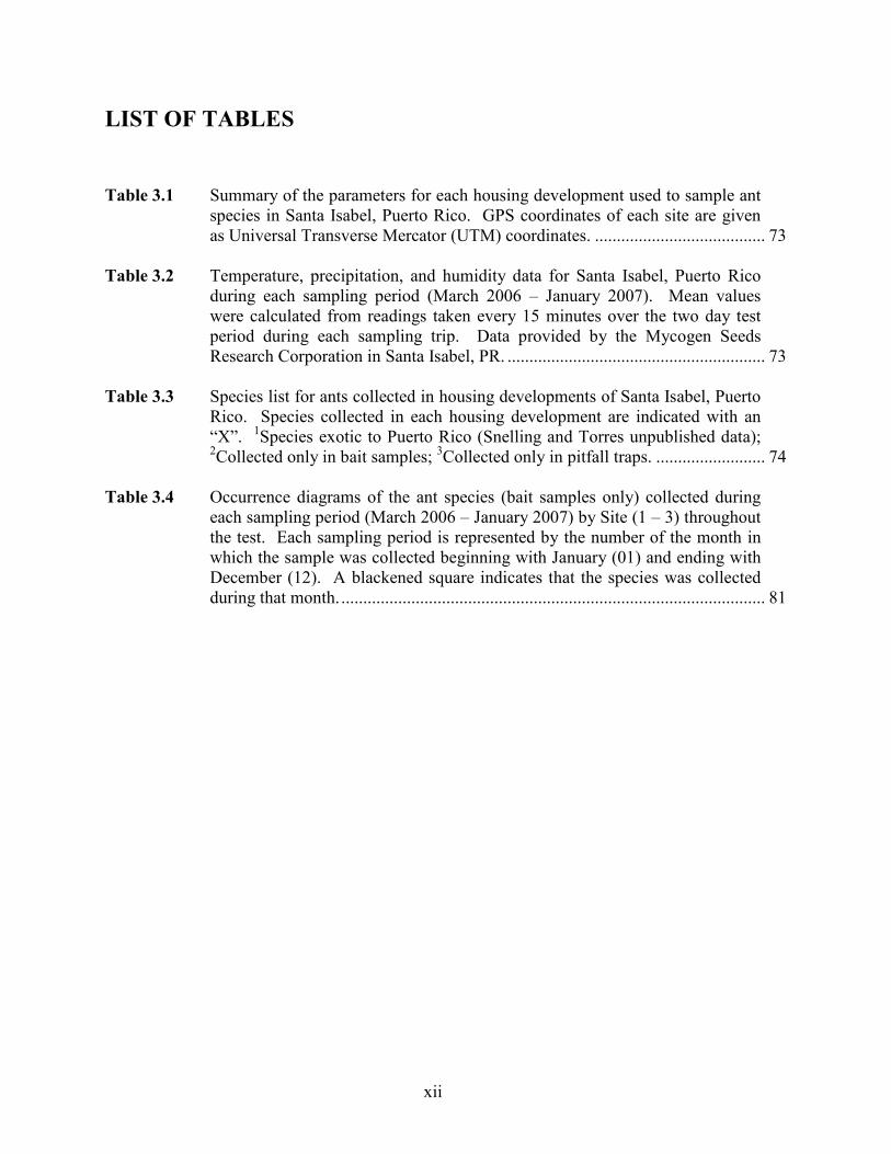
List of Tables ........................................................................................................................... xii

Chapter 1 Introduction ....................................................................................................... 1

Chapter 2 Literature Review ............................................................................................ 4

2.1 Ecological Succession............................................................................................ 4

2.1.1 Stages of Succession ................................................................................... 4 2.1.2 Mechanisms of Succession ......................................................................... 6 2.1.3 Species Diversity and Environmental Complexity ..................................... 7 2.1.4 Examples of Succession.............................................................................. 8

2.2 Urban Succession ................................................................................................ 11

2.2.1 Invasive Species and Their Impacts.......................................................... 17

2.3 Puerto Rico .......................................................................................................... 23

2.4 Pest Ant Biology .................................................................................................. 27

2.4.1 Cardiocondyla emeryi (Forel, 1881)......................................................... 27 2.4.2 Monomorium destructor (Jerdon, 1851) ................................................... 28 2.4.3 Tapinoma melanocephalum (Fabricius, 1793) ......................................... 30 2.4.4 Paratrechina longicornis (Latreille, 1802)............................................... 33 2.4.5 Pheidole megacephala (Fabricus, 1793)................................................... 36 2.4.6 Brachymyrmex spp. (Mayr, 1868) ............................................................ 39 2.4.7 Solenopsis invicta (Buren, 1972) .............................................................. 41

2.5 Statistical Methods.............................................................................................. 47

2.5.1 Basic Biodiversity Measures and Visual Representations........................ 48 2.5.2 Numeric Biodiversity Measures and Analyses ......................................... 49 2.5.3 Spatial Distribution and Analysis ............................................................. 51

vii

Chapter 3 Ant Species Composition in Housing Developments of Different Ages.................................................................................................. 57

3.1 Introduction......................................................................................................... 57 3.2 Materials and Methods....................................................................................... 60 3.3 Results .................................................................................................................. 64 3.4 Discussion............................................................................................................. 66

Chapter 4 Biodiversity of Ant Species at Three Housing Developments in Puerto Rico: Effect of Housing Development Age, Season,

Bait Type, and Time of Day ....................................................................... 85

4.1 Introduction......................................................................................................... 85 4.2 Materials and Methods....................................................................................... 87 4.3 Results .................................................................................................................. 90 4.4 Discussion............................................................................................................. 92

Chapter 5 Spatial Distribution of Ant Foraging Ranges as an Indicator of Housing Development Stage of Succession .................................... 106

5.1 Introduction....................................................................................................... 106 5.2 Materials and Methods..................................................................................... 110 5.3 Results ................................................................................................................ 110 5.4 Discussion........................................................................................................... 118

Chapter 6 Summary ......................................................................................................... 138

Literature Cited.................................................................................................................... 143

Appendix A Dates and Sampling Times for Each Sampling Trip........... 159

Appendix B Species List and Abundance of Ants Collected Using

Bait Traps ........................................................................................... 161

Appendix C Species List and Abundance of Ants Collected Using

Pitfall Traps ....................................................................................... 162

viii

LIST OF FIGURES

Figure 2.1 Biomass accumulation model of succession (Bormann and Likens 1981;

figure adapted from Molles 2005). ....................................................................... 55 Figure 2.2 Sample rank-abundance curve (figure adapted from Molles 2005)...................... 55 Figure 2.3 The 5% significance levels of χ2. If χ2 value between significance levels,

agreement with Poisson series is accepted at 95% probability level (P > 0.05; figure taken from Elliott 1971). ............................................................................ 56

Figure 3.1 Satellite image of the three housing developments used as sample sites in

Santa Isabel, Puerto Rico (March 2005; Google Earth 4.0, Google, Inc., Mountain View, CA). Although construction of Site 1 had not yet been completed when the image was recorded, construction of the entire site was finished before sampling began in March 2006.................................................... 75

Figure 3.2 Examples of typical sample houses in the one-year-old (A), four-year-old (B),

and eight-year-old (C) housing developments in Santa Isabel. ............................ 76 Figure 3.3 Example of a typical sample house in a Santa Isabel housing development.

The circles indicate the locations around the front exterior of the home where baited vials were placed to sample for foraging ants. ........................................... 77

Figure 3.4 Combined bait and pitfall trap data illustrating relative abundance (y-axis) and

total species richness (z-axis) at each housing development site. Relative abundance values for each site were calculated by dividing the number of ants collected from the site by the total number of ants collected from all three sites. ...................................................................................................................... 78

Figure 3.5 Rank-abundance curves using combined bait and pitfall data for the three

housing developments (one, four, and eight years old) in Santa Isabel, Puerto Rico. Curves are generated by plotting each ant species in descending order according to abundance. A steep slope indicates fewer species and less species evenness while a flat slope indicates a greater number of species and greater evenness. ................................................................................................... 79

Figure 3.6 Relative abundance of individual ant species (combined bait and pitfall data)

collected from each site in Santa Isabel, Puerto Rico. Relative abundance values are the proportion of ants from a single species relative to the total number of ants collected within each site. ............................................................ 80

ix

Figure 3.7 The number of species (species richness) collected during each sampling period from each housing development in Santa Isabel, Puerto Rico (bait samples only). Points on the line represent the months in which samples were collected. ............................................................................................................... 83

Figure 3.8 Ant abundance (y-axis; bait samples only) and monthly precipitation (z-axis;

TWC 2007) data for each sampling period. Points on the lines represent the months in which samples were collected from each housing development in Santa Isabel, Puerto Rico. ..................................................................................... 84

Figure 4.1 Mean number of ant species (± SE) collected from sample houses (n = 30) at

different aged housing sites (one, four, and eight years old) in Puerto Rico. Means followed by different letters are significantly different. ......................... 101

Figure 4.2 Mean number of ants (± SE) collected from sample houses (n = 30) at

different aged housing sites (one, four, and eight years old) in Puerto Rico. Means followed by different letters are significantly different. ......................... 101

Figure 4.3 Mean diversity and evenness indices (± SE) averaged across all sample houses

(n = 30) at different aged housing sites (one, four, and eight years old) in Puerto Rico. Means followed by different letters are significantly different. ... 102

Figure 4.4 Mean number of species (richness) collected at each sample house (n = 30)

during each sample period (month) from the three sites in Puerto Rico. The regression line of each site is represented by the solid black line. The slopes of the regression lines were not statistically different. ....................................... 102

Figure 4.5 Mean number of ants (abundance) collected at each sample house (n = 30)

during each sample period (month) from the three sites in Puerto Rico. The regression line of each site is represented by the solid black line. Statistically different slopes (at the P < 0.06) are indicated by a different letter located at the end of the regression line. ............................................................................. 103

Figure 4.6 Mean diversity index of each sample house (n = 30) during each sample

period (month) from the three sites in Puerto Rico. The regression line of each site is represented by the solid black line. Statistically different slopes are indicated by a different letter located at the end of the regression line. ....... 103

Figure 4.7 Mean evenness index of each sample house (n = 30) during each sample

period (month) from the three sites in Puerto Rico. The regression line of each site is represented by the solid black line. The slopes of the regression lines were not statistically different. ................................................................... 104

Figure 4.8 Mean number of species (± SE) collected from sample houses (n = 30) at

different aged housing sites (one, four, and eight years old) and bait types in Puerto Rico.......................................................................................................... 104

x

Figure 4.9 Mean diversity index (± SE) averaged across all sample houses (n = 30) at


Figure 4.10 Mean evenness index (± SE) averaged across all sample houses (n = 30) at


Figure 5.1 Simple layouts of the Puerto Rican housing development orientations used for

sampling according to adjusted UTM coordinates. Boxes represent the approximate location of houses throughout the sites while red boxes indicate houses where sampling was conducted............................................................... 128

Figure 5.2 Spatial distribution of foraging ant species collected at samples houses within

Site 1 at the beginning (March 2006) and end (January 2007) of the test. The x and y axis represent the adjusted UTM coordinates of the sample houses. The color of the circles represents the ant species collected from that location. The size of the circles represents the number of ants collected. A scale is provided to illustrate the number of ants represented by the different sizes of circles. ................................................................................................................. 129





Figure 5.5 Trends in annual population growth (abundance) and foraging distribution

(frequency) of three dominant ant species collected during each monthly sampling period within the one-year-old Puerto Rican housing development (Site 1). Note that the z-axis scale is different for each species. ....................... 132

xi

Figure 5.6 Trends in annual population growth (abundance) and foraging distribution (frequency) of three dominant ant species collected during each monthly sampling period within the four-year-old Puerto Rican housing development (Site 2). Note that the z-axis scale is different for each species. ....................... 133


(frequency) of three dominant ant species collected during each monthly sampling period within the eight-year-old Puerto Rican housing development (Site 3). Note that the z-axis scale is different for each species. ....................... 134

Figure 5.8 Spatial distribution of three dominant ant species within Site 1 collected in

March 2006, August 2006, and January 2007. The x and y axis represent the adjusted UTM coordinates of the sample houses. The color of the circles represents the ant species collected from that location. The size of the circles represents the number of ants collected. Spatial diagrams illustrate the regions of concentration and overlap of individual species foraging territories. ............ 135





xii

LIST OF TABLES

Table 3.1 Summary of the parameters for each housing development used to sample ant

species in Santa Isabel, Puerto Rico. GPS coordinates of each site are given as Universal Transverse Mercator (UTM) coordinates. ....................................... 73

Table 3.2 Temperature, precipitation, and humidity data for Santa Isabel, Puerto Rico

during each sampling period (March 2006 – January 2007). Mean values were calculated from readings taken every 15 minutes over the two day test period during each sampling trip. Data provided by the Mycogen Seeds Research Corporation in Santa Isabel, PR. ........................................................... 73

Table 3.3 Species list for ants collected in housing developments of Santa Isabel, Puerto

Rico. Species collected in each housing development are indicated with an “X”. 1Species exotic to Puerto Rico (Snelling and Torres unpublished data); 2Collected only in bait samples; 3Collected only in pitfall traps. ......................... 74

Table 3.4 Occurrence diagrams of the ant species (bait samples only) collected during

each sampling period (March 2006 – January 2007) by Site (1 – 3) throughout the test. Each sampling period is represented by the number of the month in which the sample was collected beginning with January (01) and ending with December (12). A blackened square indicates that the species was collected during that month. ................................................................................................. 81

1

CHAPTER 1. INTRODUCTION

Ants are one of the largest and most diverse groups of animals, with over 8,800 species

identified and an estimated 12,000 more undescribed species worldwide (Holldobler and Wilson

1990). Out of the thousands of described species, only a small portion, less than 0.5%, are pests

in human environments (Lee and Robinson 2001). Regardless of the small number of pest

species, pest ants have become an increasingly important group of household invaders (Lee

2002). Although pest ants are largely a nuisance, specific species such as the black carpenter ant

can cause major structural damage to homes, while the red imported fire ant can cause painful

stings resulting in allergic reactions (Ferster et al. 2000). Additionally, invasive ants have been

shown to be potential disease vectors. Lee (2002) isolated over 193 bacteria, eight species of

fungi, and two species of yeast on ants found in restaurants, cafeterias, and household kitchens.

Because of the problems (structural damage, human health impacts) associated with pest and

invasive ants, these species are an important complex to study.

The ants of Puerto Rico have been well studied over the last 100 years. Ants have been

identified as the most abundant invertebrate in Puerto Rico (Levins et al. 1973) and numerous

studies have documented the ant fauna of the island. In the past century, Wheeler (1908), Smith

(1936), Levins et al. (1973), and most recently, Torres and Snelling (1997) have catalogued the

ants of Puerto Rico. In addition to cataloguing the species, studies of the ant fauna at localized

sites around the island have been conducted by Culver (1974), Lavinge (1977), Torres (1984a,

1984b), and Osorio-Perez et al. (2007).

These studies indicate a rich fauna of ant species largely due to the subtropical climate of

the island. This subtropical climate has resulted in a greater diversity of species than in

temperate climates. The most recent survey of Puerto Rican ant species was conducted by

Torres and Snelling in 1997 where they identified 71 distinct ant species living on the main

island and surrounding keys. Many of the species collected and identified by Torres and

Snelling (1997) are well known invasive species in other parts of the world, and are considered

major pests. These species include Cardiocondyla emeryi, Monomorium destructor, Tapinoma

melanocephalum, Paratrechina longicornis, Pheidole spp., Brachymyrmex spp., and Solenopsis

2

invicta. However, the authors did not identify which of those pest species were specifically

collected in urban environments.

In general, there is very little ecological information about ants (native or invasive) in

tropical urban environments (Fowler and Bueno 1996). While there are many studies

documenting the ecology of invasive ants, these studies largely focus on natural environments

and exclude urban areas (Briese and Macauley 1977, Majer 1981, Majer 1984). Yet, invasive

ants are particularly well adapted to take advantage of urban habitats. Invasive ants, or “tramp”

ants, typically live in close association with humans and are easily dispersed by human

commerce. Tramp species typically expand their territories by budding from a central nest, and

tend to be more aggressive in taking over new habitats, often resulting in the displacement of

native ants and other invertebrates (Holldobler and Wilson, 1990). However, the community

interactions of invasive ant species in and around urban structures are not well understood

(Fowler and Bueno 1996).

To date, no studies have documented the invasive pest ant species complex of Puerto

Rico, and very little is known about their community dynamics. However, the island of Puerto

Rico provides an ideal situation to examine the community dynamics of invasive species in

urban environments. Puerto Rico has a long history of disturbance; both natural and man-made.

Additionally, the island is densely populated which has led to rapid urbanization throughout

Puerto Rico. The resulting urban habitats are ideal for the introduction of invasive ant species,

and many of the species found in these disturbed habitats are pest ants well known for their

negative impacts on biodiversity.

Until the 20th century, disturbance to the island’s landscape was almost exclusively the

result of natural events such as hurricanes and wildfires. However, in the late 20th century, the

economy of Puerto Rico underwent a major shift from agriculture (coffee, sugarcane, and cattle)

to an industrialized economy based on manufacturing and services (Lopez et al. 2001, Grau et al.

2003, Helmer 2004). This shift has resulted in the expansion of cities, and the conversion of

agricultural and forested land into residential and industrial landscapes (Lopez et al. 2001).

Due to past agricultural practices and present urbanization, broad scale human

disturbances have become a characteristic of Puerto Rican ecosystems (Aide et al. 2000, Chinea

and Helmer 2003, Grau et al. 2003). Grau et al. (2003) described Puerto Rico as a large scale

ecological experiment of almost 1 million ha that was subjected to intense human disturbance for

3

almost 100 years. As urban expansion continues, these newly developed locations are vulnerable

to invasive species of plants and animals which are adapted for life in urban habitats and can

survive in close proximity to humans.

Furthermore, the gradual urbanization of the island has produced a mosaic of urban

structures of different ages, specifically housing developments. As the environments

surrounding these housing developments recover from the disturbances associated with

construction, the environments progress through stages of urban succession. During these stages

of succession, the plant and animal communities in these urban habitats change. Therefore, the

urbanization of Puerto Rico has resulted in a mosaic of housing developments representing

different stages of succession where invasive ants are widespread and represent a major

ecological “force”. The combination of widespread invasive species and housing developments

of different ages not only represents an ideal setting to study the community dynamics of

invasive ant species, but also how these ant communities change during urban succession.

Therefore, the goals and objectives of this research project were:

1) To determine the ant species complex in housing developments of different ages and

identify the dominant species in each development;

2) To determine measures of biodiversity for each housing development, sampling

period, bait type, and time of day;

3) To determine the spatial location of the species within each housing development and

document the changes in the species’ territories over time.

4

CHAPTER 2. LITERATURE REVIEW

2.1 Ecological Succession

The word succession was derived from the Latin word successio, meaning the act or

process of following in order or sequence (Golley 1977). The term ecological succession, first

used by the French biologist Adolphe Dureau de la Malle (1825), refers to the orderly and

gradual process of change in plant and animal communities within a biome (Cowles 1911,

Golley 1977). Typically, the process of succession takes place after a disturbance to an existing

ecosystem or the formation of a new substrate (Molles 2005).

Today, ecological succession has been divided into two basic types, primary and

secondary succession. The term primary succession was first used by Clements (1916) over 100

years ago to describe the establishment and growth of a community on a barren surface lacking

any existing organisms (Marrs and Bradshaw 1993, Miles and Walton 1993, Molles 2005).

Primary succession may occur in natural or man-made environments (Bradshaw 1993).

Examples of natural environments include volcanic ash fields and lava flows, or glacier forelands

exposed after glacial retreat (Crouch 1993, Del Moral 1993, Molles 2005). Man-made

environments include locations that have been so disturbed or polluted that the physical

conditions of the land make it difficult for living organisms to become established. These

locations may have severe nutrient deficiencies, extreme soil pH values, or toxic contamination

from human activities, e.g. rock quarries, china clay sand wastes, and toxic waste dumps

(Bradshaw 1993, Marrs and Bradshaw 1993). Secondary succession describes areas where a

disturbance has occurred, destroying a pre-existing community, but without removing organic

matter from the soil (Marrs and Bradshaw 1993, Molles 2005). Like primary succession,

secondary succession may also occur in natural or man-made locations. Natural locations would

include land left barren after a forest fire, flood, or mudslide (Molles 2005). Man-made locations

would include clear-cut forests, abandoned agricultural land, or areas of urban development such

as landfills and cemeteries (Marrs and Bradshaw 1993, Molles 2005).

2.1.1 Stages of Succession

The stages of succession are highly variable depending on the type of succession

(primary or secondary) and the existing ecosystem. However, Bradshaw (1993) outlined the

5

three fundamental steps universal to the process of primary succession: arrival, establishment,

and growth. Arrival is the obvious first step. In order for arrival to occur, organisms must be in

the vicinity, available for colonization, and able to disperse to the site. Next, the newly arrived

organism must be able to become established. Selection plays an important role in the

establishment step because not all the species that arrive will survive. The founding species must

be able to tolerate and adapt to the stresses encountered in the new environment or otherwise be

eliminated (Bradshaw 1993). The group of species that are able to establish themselves in the

new terrain are known as the pioneer community (Molles 2005). The pioneer community then

progresses into the third stage of succession, the growth stage. A successful growth stage is

dependent upon two main factors, the ability of the community to acquire nutrients and a

consistent water supply. With nutrients and water, the environment is more favorable to the

growth of plants and animals, and community development begins. The growth stage leads to an

increase in species diversity which causes species interactions to occur. The interactions

between species may be beneficial or negative to any particular species but inevitably will lead

to changes in the overall species composition (Bradshaw 1993, Molles 2005).

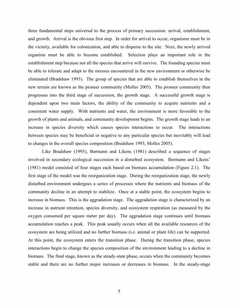
Like Bradshaw (1993), Bormann and Likens (1981) described a sequence of stages

involved in secondary ecological succession in a disturbed ecosystem. Bormann and Likens’

(1981) model consisted of four stages each based on biomass accumulation (Figure 2.1). The

first stage of the model was the reorganization stage. During the reorganization stage, the newly

disturbed environment undergoes a series of processes where the nutrients and biomass of the

community decline in an attempt to stabilize. Once at a stable point, the ecosystem begins to

increase in biomass. This is the aggradation stage. The aggradation stage is characterized by an

increase in nutrient retention, species diversity, and ecosystem respiration (as measured by the

oxygen consumed per square meter per day). The aggradation stage continues until biomass

accumulation reaches a peak. This peak usually occurs when all the available resources of the

ecosystem are being utilized and no further biomass (i.e. animal or plant life) can be supported.

At this point, the ecosystem enters the transition phase. During the transition phase, species

interactions begin to change the species composition of the environment leading to a decline in

biomass. The final stage, known as the steady-state phase, occurs when the community becomes

stable and there are no further major increases or decreases in biomass. In the steady-stage

6

phase, the community is referred to as a climax community and remains as such until another

disturbance takes place (Bormann and Likens 1981, Molles 2005).

2.1.2 Mechanisms of Succession

Regardless of the type of succession (primary or secondary), the general process of

succession relies on species moving into a previously disturbed area and modifying it. The first

species to move in (pioneer species) typically have high dispersal capabilities and grow rapidly

to reproductive maturity (Connell and Slatyer 1977). As the process of succession continues, the

pioneer species may be replaced by other organisms depending on the mechanism driving

successional change. The main three mechanisms underlying successional change are

facilitation, tolerance, and inhibition (Connell and Slatyer 1977, Molles 2005).

The facilitation model, first proposed by Clements (1916), is the most widely accepted

model. In the facilitation model, specific early-succession species are able to colonize an area.

During colonization, changes are made to the environment that makes further colonization by

similar early-succession species less suitable while making colonization by later-succession

species more suitable. In this manner, early-succession species facilitate the establishment and

growth of later-succession species while limiting the establishment of early competitors.

Eventually the species that currently inhabit the environment (resident species) cease to facilitate

the immigration of other later-succession species and a climax community is reached (Clements

1916, Connell and Slatyer 1977).

The tolerance model, like the facilitation model, begins with colonization. However,

instead of only specific early-succession species being able to colonize, any species that can

reach maturity and propagate can be a pioneer species. Like the facilitation model, the pioneer

species become established in an area and modify the environment in such a way that the area

becomes less suitable for other pioneer species. However, the environment neither becomes

more favorable nor less favorable to later-succession species. The later-succession species are

those species that tolerate the changes of the early-succession species and continue to survive

and reproduce. The climax community is achieved when the resident species are able to tolerate

the environmental modifications made by earlier species and no additional species can tolerate

the current conditions (Connell and Slatyer 1977, Molles 2005).

The third model is the inhibition model. Like the tolerance model, the inhibition model

begins with the colonization of an environment by any pioneer species able to survive and

7

reproduce in that location. The modifications caused by these pioneer species alter the

environment so that the environment is less suitable for other early-succession species as well as

later-succession species. Only when the pioneer species are killed (such as by disease or

predation), or a disturbance releases resources that were monopolized by the pioneer species, is

further colonization possible. The environment may then be colonized by the same species

again, another early-succession species, or a later succession species. If the same species or

another early-succession species colonizes the environment, the inhibition model continues

because that species continues to inhibit the establishment of additional species. However, if a

later-succession species colonizes the environment, succession begins to follow a more

traditional sequence similar to the facilitation model (i.e. later-succession species replace early-

succession species) (Connell and Slatyer 1977, Molles 2005).

Today, evidence suggests that most succession models follow the facilitation model, the

inhibition model, or a combination of both (Molles 2005). Evidence in support of the facilitation

model is most often observed in primary succession. Facilitation during glacier retreat is well

documented with the appearance of pioneer species that improve conditions, thus allowing the

colonization of later-succession species (Connell and Slatyer 1977). While it is possible that the

tolerance model for succession can occur, there have been no convincing examples or sufficient

evidence. As opposed to facilitation, inhibition models are thought to apply to secondary

succession. Many examples of secondary succession following the inhibition model have been

documented from field experiments using plants. Early-succession species of plants were

observed to reduce the rates of germination, growth, and survival of later-succession species

(Connell and Slatyer 1977). Niering and Goodwin (1974) examined secondary succession on

pastureland that had been abandoned for over 45 years. Niering and Goodwin (1974) discovered

that a closed canopy of shrubs (early-succession species) had grown on the pastureland and

prevented the establishment of tree species (later-succession species). Therefore, Niering and

Goodwin’s (1974) findings supported the inhibition model of succession.

2.1.3 Species Diversity and Environmental Complexity

Species diversity can be defined as the number of species coexisting and their relative

abundance within a community. The number of species in an environment is referred to as

species richness while the relative abundance of species is called species evenness (Molles

2005). In general, species diversity is higher in more complex environments. Because

8

succession, regardless of the type or mechanism, typically results in an increase of the

environmental complexity, community changes will increase the species diversity over time

(Molles 2005).

Multiple studies have examined the relationship between environmental complexity and

species diversity. Primary successional studies focusing on areas of glacial retreat examine the

environmental complexity in terms of nutrients and soil depth. Chapin et al. (1994) studied the

major successional stages at Glacier Bay, Alaska to determine the potential causes of

successional change. Chapin et al. (1994) examined four stages based on the prominent plant

species present: (1) pioneer species (including blue-green algae, lichens, liverworts, and

Epilobium latifolium L.), (2) Dryas shrubs, (3) Adler trees, and (4) Spruce trees. It was

discovered that the growth of most plant species was limited in the pioneer stage due to low

amounts of nitrogen and phosphorus. However, as succession proceeded from the Dryas to adler

stage, the availability of nutrients increased. Increased inputs of organic matter and nitrogen

were primarily due to the addition of adler litter. The increase of inputs continued into the

spruce stage where the soil properties of organic matter, moisture, and nitrogen reached their

greatest levels (Chapin et al. 1994). MacArthur and MacArthur (1961) conducted a similar study

where they compared the species diversity of birds in forest sites of increasing complexity and

foliage height. The results of the MacArthur and MacArthur (1961) study documented a positive

correlation between increased foliage height and bird species diversity.

2.1.4 Examples of Succession

On May 18, 1980, Mount St. Helens erupted, spreading over 50 million cubic meters of

volcanic material over a wide arc extending out 18 km from the crater (Del Moral 1993). The

blast devastated almost 600 km2 of forests. A 20 km2 section of forest just north of the volcano

was completely destroyed during the eruption. This 20 km2 section of the forest, now known as

the pumice plains, was covered with hot ash and pumice that killed all plant life. The barren

pumice covering that remained set the stage for a carefully planned study on primary succession

(Molles 2005)

The mechanisms of primary succession on Mount St. Helens were studied by William

Morris and David Wood (1989). Morris and Wood (1989) examined the succession of three

plant species, lupine (Lupinus lepidus), pearly everlasting (Anaphalis margaritacea), and

fireweed (Epilobium angustifolium) on the pumice plains. Lupine, which is able to increase the

9

nitrogen levels in the soil, was the pioneer species on the plains. Morris and Wood (1989)

studied the effect of lupine on the pearly everlasting and fireweed. Morris and Wood (1989)

discovered that lupine had an inhibitory effect on the seedling establishment and survival of the

pearly everlasting and fireweed. A higher percentage of pearly everlasting and fireweed

seedlings survived on the barren pumice fields than on those sections of the fields where lupine

was present. However, those seedlings that were able to survive in the presence of lupine grew

to a larger and healthier size than those seedlings that established on the barren sections of the

fields. Morris and Wood (1989) determined that the healthier pearly everlasting and fireweed

seedlings where lupine was present was attributed to the increased nitrogen available in the soil.

Therefore, lupine was determined to facilitate the growth of the pearly everlasting and fireweed

seedlings. Thus, the Morris and Wood (1989) study supported both the inhibitory and facilitative

models of succession in that lupine inhibited seedling establishment but facilitated seedling

growth (Molles 2005)

Another study that examined primary succession on volcanic substrates around Mount St.

Helens was conducted by Del Moral (1993). Del Moral (1993) selected plots made up of four

different substrates (lahars, the blast site, the scoured site, and a tephra site). The lahars site was

covered by water-saturated debris (i.e. volcanic material, mud, and vegetation). This debris had

covered the landscape after intense heat caused the glaciers on Mt. St. Helens to melt rapidly and

create a mudflow. The blast site had been directly exposed to the eruption and was characterized

as a barren plot subjected to intense heat and severe soil removal. The eruption had also caused

soil removal on the scoured site, but the scoured site did not experience the intense heat of the

blast site. The tephra site was covered in a substrate formed from airborne volcanic material

such as ash and cinders. Each plot within a particular site was 250 square meters. The species

richness of these plots was then recorded each year for ten growing seasons. Although the

species richness was different on each substrate, Del Moral (1993) discovered that species

richness increased on every substrate over the ten year study. Additionally, the species richness

of two substrates (the tephra site and the scoured site) reached a steady state equilibrium within

three to four years after the eruption (Del Moral 1993).

Classic studies on secondary succession were conducted by Henry J. Oosting (1942) and

David Johnston and Eugene Odum (1956) in the Piedmont Plateau of North Carolina (Molles

2005). During the past three centuries, deciduous forests in eastern North American have been

10

extensively cleared and cultivated for agriculture. Over time, the older agricultural fields were

deserted as new sections of land were deforested, leaving the landscape covered by abandoned

fields of various ages (Oosting 1942, Johnston and Odum 1956, Molles 2005). Oosting (1942)

studied the succession of woody plants invading these fields. In one study, Oosting (1942)

compared the species richness of abandoned fields and forest stands of different ages. The fields

had been abandoned one, two, three, and five years previously. The forest stands studied were

11, 22, 31, 34, 42, 75, and 110 years old, and a climax forest (150 years old). The number of

woody plant species was counted in each field and forest stand. Oosting (1942) found that there

were no species of woody plants in the agriculture fields that had been abandoned for one or two

years. However, in the three year old and five year old fields, loblolly pine seedlings had begun

to appear and grow. In the 11-year-old-forest stand, pine seedlings had grown to a size where

they formed a closed canopy over the fields. The closed canopy inhibited the growth of younger

pines while facilitating the growth of young hardwood trees which resulted in a rapid increase

from one to nearly 40 species of woody plants. Oosting (1942) compared the forest stands

ranging from 22 to 110 years old and discovered that oak and hickory became the dominant

species. However, as the forest stands increased in age, the number of pines slowly decreased.

The resulting climax community consisted of hardwood stands which contained four distinct

classes of vegetation, the overstory, understory, saplings (between one and ten feet tall), and

seedlings (< one foot tall). Oosting concluded that secondary succession in the Piedmont of

North Carolina reached a climax community in 150 years and contained 50 to 60 species of

woody plants (Oosting 1942, Molles 2005).

In 1956, Johnston and Odum (1956) followed in the footsteps of Oosting (1942) by

studying the succession of bird species across a range of vegetation. Johnston and Odum (1956)

selected 13 plots that were classified as grassland (one to three years old), grassland-shrubland

(15-20 years old), pine forest (25-100 years old), or hardwood forest (150-200 years old). The

results determined that only two species of birds were present in the grassland plots. However,

diversity increased to between eight and thirteen species in the grassland-shrubland plots.

Species richness peaked in the pine forests after 50 years of forest succession. Johnston and

Odum (1956) found a climax community of about 24 species of birds in hardwood forests 100-

150 years old (Johnston and Odum 1956, Molles 2005).

11

2.2 Urban Succession

While most studies on ecological succession focus on natural communities, urban

succession focuses on successional processes that take place in urban ecosystems. Urban

ecosystems vary in size and complexity, and therefore contain many different ecological niches.

Urban ecosystems include residential lawns and gardens, industrial sites, abandoned properties,

parks and play grounds, cemeteries, waste disposal sites, forests, fields, and bodies of water

(Nagle 1999). Succession in natural environments may be caused by natural or man-made

disturbances. However, urban succession only occurs after human disturbances, which typically

happen during the process of urbanization. During urbanization, vegetation is removed and the

soil is graded. This process leaves a barren substrate where urban succession can occur. Plants

and animals slowly reestablish in the disturbed ecosystem causing species diversity to increase

(Rebele 1994). However, the method by which the urban ecosystem reestablishes (i.e. the

process of succession) depends on how the land is used. Typically, the disturbed ecosystem is

either abandoned or continues to be affected by humans.

When an urban ecosystem is abandoned, the process of succession on that abandoned

land is heavily influenced by the surrounding environment (Prach et al. 2007). When abandoned

urban ecosystems are in close proximity to natural ecosystems, succession follows a traditional

pathway and the disturbed area can return to a natural state relatively quickly. Early successional

species are able to come from nearby undisturbed sites and establish in the abandoned space

(McIntyre 2000). Landfills and other large waste disposal sites are often surrounded by natural

ecosystems. These landfills are soon colonized from the surrounding habitats by early

successional plants which are tolerant of harsh conditions, such as reduced soil nutrients, low soil

moisture content, and chemical contamination. The early successional species are replaced by

later successional species of plants (often perennials) in a traditional successional progression

(Nagle 1999). Soon after vegetation has become established, animals from nearby undisturbed

habitats colonize the area. Early succession animal species are typically scavengers and

opportunistic generalists that take advantage of the microhabitats. Birds, small rodents, and

insects are all common early successional invaders (Nagle 1999). As succession progresses to

later stages, plant diversity and complexity increases. This increase allows the disturbed habitat

to support a larger diversity of animals. The disturbed lands then begin to resemble the

surrounding natural environment (McIntyre 2000).

12

Instead of being surrounded by a natural environment, abandoned land is often

surrounded by an urban landscape. Because the land is isolated from any natural ecosystem, the

successional process takes much longer. Grassland communities can take 20-30 years to develop

in urban locations, and over 100 years may be required for the abandoned land to progress to a

forest-like environment (Mitich 1992). Weedy species tend to be the initial colonizers in urban

locations rather than natural early-succession species. These weedy species have the advantage

of being easily dispersed by the wind or animals. The weeds grow to reproductive maturity

quickly and produce a large numbers of seeds. By producing many seeds, these weedy species

are able to quickly establish and proliferate in disturbed urban habitats (Mitich 1992).

Santamour (1983) examined the succession of plants in abandoned urban brickyards.

The brickyards were built in 1909 and active until they closed in 1972. Santamour (1983)

conducted a survey of the plant species that had become established in the brickyard 10 years

after abandonment. Santamour (1983) found that in locations where organic matter had

difficulty building up, plant growth and succession was severely slowed. These locations were

mainly located on the top and crowns of the brick kilns. Pioneer species were the only plants on

the tops of the brick kilns and were likely the first plants established in the brickyards. The

pioneer species were composed of annual herbs and grasses which produced small seeds that

could be easily dispersed by the wind. Other locations in the brickyard where plants had become

established included the shoulders and bases of the kilns. In these locations, woody species of

plants were found. Santamour (1983) concluded that the early pioneer grasses and herbs were

able to colonize the shoulders and bases of the kilns quickly. Then, when these grasses died and

decayed, a nutrient base layer of soil built up for later succession plant species. A total of 16

different genera of plants were identified in the brickyard. Most of the genera were considered

“weed trees” such as Ailanthus (Tree of Heaven) that had small seeds which were easily spread

by the wind. Santamour’s (1983) findings suggest that successional species in isolated urban

habitats tend to be invasive or weedy because weedy species travel easily to isolated habitats via

wind dispersal.

Another study examined urban succession in a disturbed site that had been abandoned for

at least 20 years. De Wet et al. (1998) studied an abandoned industrial site that had been

subjected to various types of disturbance and was surrounded by residential and commercial

developments. The location had been used for different purposes at different times in the site’s

13

history and different locations on the site revealed a complex assortment of successional

recovery stages. Sections of the site were categorized into three main types of impact based on

the location’s history: building areas, mining areas, and landfills. Succession in building areas,

specifically abandoned brick making locations, was similar to that described by Santamour

(1983) and determined to be relatively slow. Only a few well rooted plants were found in the

building areas, and only a thin nutrient layer was present for plant establishment. The plants that

were established consisted mainly of weedy species. In mining areas, plant growth was highly

variable. Most of the mining surface consisted of exposed rock on which the soil cover had been

removed. Therefore, plant establishment in these locations was also difficult. The beginnings of

ecological succession were observed only in areas where the soils were deep enough to support

plant life. The landfill sections of the site were also recovering so slowly that little to no plant

growth was observed. The landfills had been filled with compacted trash and covered with a thin

layer of soil. Therefore, the compacted refuse prevented plants from penetrating into underlying

soil. The trash also failed to hold water, creating a low moisture environment for plant

establishment. De Wet et al. (1998) concluded that succession throughout the entire site had

been slowed due to the disturbance history of the site which created harsh conditions for plant

establishment. Succession at the site had also been impeded because of the surrounding urban

developments which inhibited the introduction of native plant species.

Although some disturbed urban habitats are disturbed and abandoned, other urban

habitats continue to be affected by human activities. Unlike succession on abandoned lands,

succession in these repeatedly disturbed habitats depends on the type of human disturbance more

than the surrounding environment. Typically, the impact of disturbance either facilitates or

inhibits natural succession of both plants and animals. Facilitative impacts aid in the

successional process and can cause it to speed up (Robinson and Handel 1993). Examples of

facilitative human impacts include covering landfills with soil or planting vegetation in cleared

areas. Inhibitory impacts disrupt the environment causing natural succession to be delayed.

Inhibitory impacts usually involve reoccurring disturbances like mowing an area on a regular

basis.

In order to restore the beauty or use of a disturbed location, humans may attempt to

facilitate the successional process by planting native vegetation in a recovering site. Robinson

and Handel (1993) examined restorative plant succession on landfills in the northeastern United

14

States. Typically, succession on the landfills resulted in a landscape of weedy species

characteristic of abandoned lands surrounded by urban environments. Robinson and Handel

(1993) attempted to facilitate the restorative process by adding clusters of native trees and shrubs

to the landfill. A total of 3,000 shrubs and 500 trees from 18 different species were planted

across three sites. The sites were surveyed a year later to determine if and how the native species

were aiding natural succession. The survey focused on finding and identifying new species of

seedlings to determine how the seedlings may have been delivered to the site. Robinson and

Handel (1993) found that survival of the native species was high (17 out of 18 species).

However, from the 17 surviving species, only about 20% of the plants were reproductive and

contributed very few seedlings to the landfill recovery. Nearly all the new species of seedlings

(95%) came from sources outside the landfill. A total of 32 new plant species were identified.

Nine new species of seedlings were wind dispersed and of those nine, four represented invasive

species. The majority of new seedling species (20 species) were dispersed by animals (i.e. birds

and mammals). Birds were determined to be the main seed disperser because they feed on fleshy

fruits and ingested the seeds outside the landfill area. The birds would then fly to the landfill

and perch in transplanted trees. Seeds would then be dropped into the landfill in the birds’

excrement.

At a similar site where no facilitative planting was done, new species of plants were

dispersed into the site by both wind and animals. However, at the non-facilitated site, the

number of new species and the total number of new plants were eight times lower than that of the

facilitated site. Robinson and Handel’s (1993) findings indicated that restorative efforts speed

up the succession process by increasing the species richness and complexity of a disturbed site.

Thus, restorative planting allows wildlife habitats and biodiversity to increase relatively quickly.

The recolonizing efforts of animals in abandoned sites undergoing human facilitated

succession have also been studied. Bioindicator species such as ants and other invertebrates are

often the target of studies in these recovering habitats. Majer (1981) examined the species

richness of ants and other invertebrates at sites formerly used for mining. Two mining sites were

selected for sampling: one human facilitated site had been seeded with native plants while the

other site was completely abandoned. Majer (1981) discovered that more species of ants and

other invertebrates were found on mining sites where native vegetation had been planted. Majer

(1984) later compared the ant species richness of mining sites which had been seeded to that of

15

mining sites that were planted with nursery reared trees. The results of the study indicated that

there was no significant difference in ant recolonization between the two sites. However, in the

early stages of succession seeded sites had more diversity and abundant ant fauna than the sites

with planted trees. Yet, 3.5-7.5 years after revegetation, both types of sites had ant species

richness values that were similar to those of the forests surrounding the sites.

Although human facilitated succession helps to speed up the process of natural

succession, human impacts can also be inhibitory. Inhibitory impacts include mowing, burning,

fertilization, heavy watering, and trampling (Bastl et al. 1997). These types of activities cause a

series of reoccurring disturbances to “recovering” habitats. Therefore, the habitat is unable to

reach a natural climax community that is similar to the surrounding undisturbed habitats and

instead remains in the early stages of succession (MacKay 1993). Because of these repetitive

disturbances, the conditions in these disturbed locations can be harsh and unfavorable for the

establishment of native species. Instead, these conditions often favor the establishment of

invasive species that are able to persist in the wake of repeated disturbances (McIntyre 2000).

Not surprisingly, it is in these locations of repeated inhibitory disturbance that invasive species

are the most prevalent.

MacKay (1993) studied ant succession in a low level nuclear waste site subjected to

repeated human disturbances. The nuclear waste site was mowed at irregular intervals while

adjacent native vegetation remained undisturbed. Ant species were sampled throughout the

nuclear waste site on four mowed plots and one plot in the undisturbed vegetation. MacKay

(1993) found that the composition of the ant community in the mowed plots was different than

the ant community in the adjacent undisturbed vegetation. Many initial colonizers in the mowed

plots were described as invasive species commonly found in surrounding urban environments of

the county. These invasive species were not commonly found in the undisturbed plot.

Additionally, the mowed plots lacked seven species that were collected in the undisturbed plot.

MacKay (1993) determined that these seven species were not present in the mowed plots due to a

lack of suitable nesting locations such as rocks, rotting logs, and pine needle beds. However, the

author concluded that native plants, trees, and other ant species would be able to colonize the

mowed plots, if the mowing stopped. In other words, the nuclear waste site would follow a more

natural succession pathway, resulting in a community similar to the surrounding native

vegetation, if the repeated mowing was discontinued.

16

In Perth, Western Australia, Majer and Brown (1986) examined the ant fauna within

residential gardens. The gardens were exposed to repeated human disturbances such as regular

mowing, trampling, watering, and the application of pesticides. Ants were sampled in the

gardens and compared with samples collected by Rossbach and Majer (1983) in the surrounding

woodlands and open-forests. Majer and Brown (1986) discovered that the ant species complex

in the gardens was lower in both richness and diversity than in the surrounding woodlands. A

total of 47 species were collected in the gardens. Out of the 47 ant species, 24 species (51%)

were not found in the surrounding woodlands. Majer and Brown (1986) concluded that the 24

species had a preference for disturbed habitats (gardens). In contrast, 60 species were collected

in the surrounding woodlands, yet only 23 species were also found in the gardens. Therefore, 37

woodland species (62%) did not colonize the disturbed gardens. Majer and Brown (1986)

concluded that the lower species richness in the gardens was caused by the inability of many ant

species to colonize the disturbed habitats.

To summarize, urban succession generally takes place in habitats that are completely

abandoned or in habitats where human activities continue to impact the environment. In

abandoned lands, the surrounding environment determines the progress and composition of

succession. Succession in abandoned lands that are in close proximity to natural environments

follows a natural progression until the disturbed habitat mimics the natural surroundings. If

invasive species are able to colonize the area, their impacts are minor and typically the invasive

species fail to remain in later successional stages. When abandoned lands are surrounded by an

urban environment, succession is slowed, and the establishment of invasive species is favored

over native species. Therefore, succession follows an unnatural progression and invasive species

tend to dominate the different stages of succession. When humans repeatedly impact disturbed

environments, the type of human impact determines the successional process. If the human

impacts are facilitative, succession can follow a natural progression. Species richness and

biodiversity quickly increase and later are influenced in composition by the surrounding

environment. Invasive species may initially invade but have difficulty surviving in the later

stages of succession. When human impacts are inhibitory, natural succession is prevented by the

continued disturbance. The environment remains at the early stages of succession, which favors

invasive species and often excludes native species. Therefore, an understanding of the

17

surrounding environment and the type and frequency of human impact is important for

predicting what type of species will be favored in urban succession situations.

2.2.1 Invasive Species and Their Impacts

Invasive species are described as those species which have established themselves

outside of their natural habitats. Invasive species often have few natural enemies outside their

native range so they spread quickly resulting in many negative environmental impacts as they

begin to dominate the invaded habitat (Colautti and MacIsaac 2004). The studies on urban

succession previously discussed indicate that disturbance favors invasive species. When

succession follows a natural progression, invasive species only play a minor role in the early

stages of succession. Environments with high diversity (usually a result of natural succession)

are typically more resistant to invasive species. Therefore, the presence of many native species

has been found to reduce the impact of invasive species by resisting invasion and protecting the

natural succession patterns (Mandryk and Wein 2006).

Urban habitats are disturbed environments. Urban habitats usually have low diversity

because the disturbances inhibit natural succession and the establishment of native species.

Therefore, invasive species are able to play a dominant role in succession and have major

impacts on the disturbed habitat (Nagle 1999). Invasive species have biological advantages over

native species that allow them to survive and proliferate in disturbed areas (Tsutsui and Suarez

2003). Invasive species are able to easily disperse into disturbed locations. Many invasive

plants have adaptations to allow for dispersal by the wind. These adaptations include having

small, light weight seeds, seeds with hairs, and seeds with parachute-like appendages (i.e.

dandelions) (Mitich 1992).

Invasive animals are also dispersed into disturbed areas by human activities. Humans

often inadvertently transplant invasive animals when transporting landscaping materials, top soil,

and shipping containers. Once transported to the new environments, invasive species are highly

adapted to establish in the disturbed habitats that may have only limited resources. For example,

many invasive animal species usually have an omnivorous diet and few nesting requirements,

thus allowing them to make use of less than optimal food resources and limited harborages

(Holway et al. 2002, Walters 2006).

The significance of invasive species (plant and animal) is the detrimental effect they have

on the environment once they have become established. After establishment, invasive species

18

grow quickly to reproductive maturity. Their rapid growth and reproduction allows for prolific

spreading, resulting in competitive dominance (Mitich 1992, Walters 2006) and the displacement

of native species (Allendorf and Lundquist 2003). Invasive species are recognized as a great

threat to global biodiversity, second only to habitat loss and fragmentation (Allendorf and

Lundquist 2003).

In addition to the negative impacts on biodiversity, invasive species negatively affect the

natural process of succession. When a habitat is dominated by invasive species, succession

follows a pathway that is different from that of a natural ecosystem (Allendorf and Lundquist

2003, Mandryk and Wein 2006). In balsam-fir forests of the Southern Appalachians, the balsam

woolly adelgid (Adelges piceae) was found to alter natural forest succession by destroying later

successional species of Fraser firs (Pimentel et al. 2000). The death of these fir trees has caused

a drastic change in the local forest composition. Traditional vegetation consisting of blueberry

bushes and fir saplings were replaced by blackberry, red spruce and yellow birch plants. This

alteration in the natural succession process also resulted in the loss of two native bird species, a

spruce-fir moss spider, and a federally endangered species of endemic lichen (Rabenold et al.

1998).

Finally, invasive species also represent significant costs to the global economy. Pimentel

et al. (2000) estimated that the cost associated with economic losses and environmental damage

due to invasive species in the United States alone is over $138 billion a year. An example of the

costs associated with invasive species is the damage and control costs associated with a single

species of mussel, the zebra mussel (Dreissena polymorpha), which exceeds $5 billion annually.

These invasive mussels monopolize food and oxygen in aquatic habitats causing a reduction in

the native fauna. In high densities, zebra mussels also clog water intake pipes and water

filtration systems.

Invasive species include a broad range of organisms (plants, mammals, mollusks, and

insects). Of the many invasive species, ants comprise some of the most widespread and

damaging invaders (Tsutsui and Suarez 2003). While some ants invade natural environments,

the majority of invasive ants establish in human modified environments and urban habitats.

These ant species, commonly referred to as tramp ants, have characteristics of typical invasive

species which allow them to disperse, establish, and proliferate in urban habitats (Holway et al.

2002, Tsutsui and Suarez 2003).

19

Tramp ants typically live in close association with humans, and therefore are easily

dispersed by human commerce. Currently, tramp ant species are located on every continent

except Antarctica. Once introduced to a new habitat, tramp ants quickly establish because of

their ability to nest in many different locations; in the soil, under stones, in plant and tree

cavities, and in man-made structures (Smith 1965). These colonies can quickly increase their

numbers due to polygyny (multiple queens). Once the ant colonies have developed a large

number of workers (1,000s to 100,000s), tramp species expand their territories by budding from

the central nest. Budding enables the colony to rapidly spread throughout the new location. The

result of this spreading is the monopolization of resources, and the displacement of native ants

and other invertebrates in the habitat (Holldobler and Wilson 1990, Tsutsui and Suarez 2003).

One unique aspect of tramp ants as compared to other invasive organisms is their

unicoloniality. Unicoloniality is the phenomenon that occurs when different colonies of the

same species form interconnected nests. These nests contain multiple queens, and the workers

cooperate with each other. Although there is no aggression between the same species, tramp ants

tend to be more aggressive in taking over new habitats from other species. The intracolony

cooperation results in supercolonies of a tramp species dominating large tracts of disturbed

habitat (Tsutsui and Suarez 2003).

Tramp ants cause many different destructive effects on invaded environments. Because

tramp ants are aggressive and can out-compete other organisms, many studies have shown their

direct impact on biodiversity. Tramps ants cause a reduction in the number of native ants and

other invertebrates in the habitat resulting in a decrease in species abundance and diversity

(Walters 2006).

Native invertebrate species have many roles in the natural environment, acting as

predators, scavengers, herbivores, granivores, and as prey for other invertebrates, reptiles, and

birds. If these native species are removed, the result can have far reaching environmental

impacts causing permanent alternations to the ecosystem (Holway et al. 2002). For example,

native ant species have mutualistic relationships with other organisms, specifically plants. Some

plants rely on ants as seed dispersers. The seeds have lipid rich appendages that the native ants

need as a food source. In return, the ants disperse and bury the seeds (Ness and Bronstein 2004).

Native ants also provide protection for plants. Plants may produce nectar as a food source for the

ants and in return, the ants defend the plant from other arthropods that feed on the leaves or

20

phloem. These mutualistic relationships are disrupted when native species are displaced by

tramp ants. Instead of dispersing seeds, many invasive ants feed on the seeds. Instead of

protecting plants, tramp ants rear and tend phytophagous insects that feed on the plants.

Therefore, tramp ants can disrupt native invertebrate communities and cause substantial indirect

impacts on vegetation and other organisms (Holway et al. 2002, Ness and Bronstein 2004).

Two of the most damaging and well studied species of tramp ants are Linepithema humile

(the Argentine ant) and Solenopsis invicta (the red imported fire ant). Both of these species

exhibit tramp ant characteristics and have major effects on the habitats they invade (Tsutsui and

Suarez 2002).

The Argentine ant is a worldwide invasive species that has spread to six continents and

many oceanic islands (Suarez et al. 2001). Argentine ants are highly unicolonial and often form

supercolonies of extremely high densities covering vast areas of land (Suarez et al. 1999). In a

Louisiana orange grove, trapping yielded over 1.3 million Argentine ant queens in a single year.

The total volume of ants collected was reported to be over 1,000 gallons (Horton 1918).

Wherever they are introduced, Argentine ants are often associated with the loss of native ants

and other invertebrates because of their vast colony numbers (Walters 2006). In the Hawaiian

Islands, the Argentine ant has been associated with reduced native and non-native arthropod

populations. Many native arthropods are unique to the islands. The endemic Lycosa hawaiiensis

(Lycosidae), a large wolf spider, is an important predator species and Agrotis sp. (Noctuidae) is

an important pollinator of the native plants. Locations where Argentine ants are present had

reduced populations of the wolf spider larvae, Agrotis sp., as well as other endemic insects,

including species of Diptera and rare flightless Colleoptera (Cole et al. 1992).

Argentine ants have also been reported to affect vertebrate populations. In southern

California, Laakkonen et al. (2001) studied the impacts of Argentine ants on native shrew

communities. In the study, Argentine ants were found to have a significant negative impact (P <

0.001) on the abundance of the shrew species, Notiosorex crawfordi. However, the specific

reasons for the decreased abundance of shrews in the presence of Argentine ants were not

determined.

The impacts of Argentine ants on plants and vegetation have also been well documented.

In 2003, a study was conducted to examine plant seed dispersal and germination in locations

where Argentine ants were present. Gomez et al. (2003) studied the fleshy fruit plant Rhamnus

21

alaternus along the Mediterranean coast in Spain. Gomez et al. (2003) determined that habitats

invaded by Argentine ants had a reduction in the number of seeds that were dispersed, the

distance over which the seeds were dispersed, and the number of seedlings that emerged

compared with other locations. Argentine ants also damage plants indirectly by tending

honeydew excreting Homopterans (Lach 2003, Ness and Bronstein 2004, Daane et al. 2007).

These Homopterans cause economic damage to fruit crops by secreting honeydew that ruins fruit

and aids in plant disease transmission. Daane et al. (2007) found that Californian vineyards

infested with Argentine ants experienced increased populations of the obscure mealybug,

Pseudococcus viburni. Population densities of the grape mealybug, Pseudococcus maritimus,

also increased due to tending by Argentine ants. However, parasitoid populations

(Pseudaphycus flavidulus and Leptomastix epona) that typically prey on the mealybugs were

lower in the same Argentine ant infested vineyards, indicating that Argentine ants reduced

parasitoid populations. The reduced parasitoid populations further allowed mealybug

populations to increase and damage larger numbers of plants (Daane et al. 2007).

In a recent study, Walters (2006) studied the effects of Argentine ants in urban parklands.

The parkland sites were all urban habitats that had been subjected to continued human

disturbance in the form of mowing and sprinkler irrigation. Eight parkland sites were selected

for sampling. Half of the sites (four sites) that were sampled had been invaded by Argentine ants

while the other four sites did not have established Argentine ant colonies. Sampling where

Argentine ant colonies were established yielded over 21,000 Argentine ants but only about 1,000

other ants. In areas where Argentine ants were not present, over 40,000 other ants were

collected. Disturbed sites without Argentine ants also had greater species richness. Nine genera

of ants were captured in non-Argentine ant infested sites, but none of these genera were found

where Argentine ants were present. Therefore, Walters (2006) concluded that Argentine ants

caused reductions in non-Argentine ant abundance and diversity.

Like the Argentine ant, the environmental effects of red imported fire ant invasions are

well documented and often devastating. Red imported fire ant (RIFA) invasions have negative

impacts on human health, livestock, wildlife, and crops (Morrison et al. 2004). Many of these

effects are discussed in a later section on RIFA and their biology, but a few studies on RIFA

invasion are discussed here. Similar to Argentine ants, RIFA have many impacts on agriculture

and biodiversity. Lofgren (1986) reported that RIFAs cause direct damage to crops. Adams et

22

al. (1983) found that soybean yields were significantly reduced in RIFA infested fields. The

reduced soybean yields were directly associated with RIFAs feeding on the germinating seeds

and seedling. In addition, indigenous arthropods and other native wildlife have been displaced

by RIFA predation (Lofgren 1986). These affected species include snails, bobwhites, alligators,

sea turtles, rodents, and many arthropod species (Holway et al. 2002).

However, RIFA are also known to facilitate the population growth of some insect pest

species by reducing their predator populations (Kalpan and Eubanks 2002). The relationship

between RIFAs and the cotton aphid has been well researched. Cotton aphids are a major pest of

cotton. The aphids cause damage to the plant by feeding on leaves, spoiling the cotton lint by

excreting honeydew, and transmitting plant diseases and viruses (Henneberry et al. 2000). In

east Texas, aphid population densities were found to have a strong positive correlation with the

presence of RIFA (Reilly and Sterling 1983). A study by Diaz et al. (2004) found that cotton

fields in north and central Texas where RIFA were not controlled, densities of the cotton aphid

were significantly greater than in fields where RIFA was controlled (P < 0.001). Although aphid

densities did not reach economic thresholds, RIFA were still determined to have a positive

influence on the population growth of cotton aphids due to RIFA reduction of cotton aphid

predators (Diaz et al. 2004, Kalpan and Eubanks 2002). Kalpan and Eubanks (2002) found that

in greenhouse and field experiments, red imported fire ants reduced the survival of lady beetle

larvae (Coccinella septempunctata and Hippodamia convergens) and green lacewing larvae

(Chrysoperla carnea). The reduction of these cotton aphid predators corresponded with a two-

fold increase in the survival rate of cotton aphids.

Multiple studies have documented the ability of RIFAs to decrease the biodiversity of

invaded environments by displacing other ant species (Porter et al. 1988, Banks and Williams

1989, Porter and Savignano 1990, Mann 1994, Pennisi 2000). A well documented study of

native arthropod communities affected by polygyne RIFA was conducted by Porter and

Savignano (1990). The study was conducted at a field station in central Texas where RIFAs

were becoming established. Porter and Savignano (1990) sampled the field station for five years

to document any changes in the abundance and species richness of the arthropod community.

The impacts on abundance, diversity, and species richness were extreme. The species richness

of native ant fauna dropped 70% and the number of individual native ants collected decreased

90% during the experiment. Other arthropods (isopods, tumblebug scarabs, and erythraeid

23

mites) were also significantly affected. The species richness of these arthropods decreased by

30% while their abundance decreased by 75% in infested areas.

A more recent study by Cook (2003) found that RIFAs similarly affected the species

richness of native ants of Texas. During a three year study in central Texas, Cook (2003)

determined that plots where RIFAs were controlled had significantly higher species richness than

plots where RIFAs were untreated. Of the 11 species initially found in plots where RIFA were

invading, only seven species remained after three years. However, in plots where RIFAs were

treated with hydramethylnon (0.73%, Amdro Fire Ant Bait, Ambrands, Atlanta, GA) or

methoprene (0.5%, Extinguish Professional Fire Ant Bait, Zoecon, Schaumburg, IL) the number

of species collected increased from 12 to 13 during the same time period.

Argentine ants and red imported fire ants are two well studied species of tramp ants that

have major effects on biodiversity. However, many other tramp ant species have been

documented to have similar impacts. Big-headed ant (Pheidole megacephala), little fire ant

(Wasmannia auropunctata), and crazy ant (Anoplolepis gracilipes), have all been shown to

negatively impact the environments into which they have been introduced (Holway et al. 2002).

Although these species can affect natural communities, their impacts are the most severe in

disturbed habitats.

2.3 Puerto Rico

The island of Puerto Rico provides an ideal situation to document the effect of invasive

species on natural biodiversity. Puerto Rico has a long history of disturbance; both natural and

man-made. Additionally, the island is densely populated which has led to rapid urbanization

throughout Puerto Rico. The resulting urban habitats are ideal for the introduction of invasive

ant species, and many of the species found in these disturbed habitats are pest ants well known

for their negative impacts on biodiversity.

Puerto Rico is located in the Caribbean Sea at 17° 45’ N, 66° 15’ W. Puerto Rico is the

smallest island within the Greater Antilles with a total area of approximately 8900 km2 (Grau et

al. 2003, Helmer 2004). Due to Puerto Rico’s location, the island’s climate is mostly Tropical

Marine with a mean annual temperature between 19° C and 26° C. Annual precipitation on the

island ranges from 900 mm on the drier southern coast to 5000 mm in the mountainous interior

(Grau et al. 2003). The dry season in Puerto Rico lasts from December to April while the wet

24

season runs from May to November. During the wet season, the mean monthly rainfall increases

from about 89 mm to 154 mm, partly due to hurricanes in the Caribbean (NOAA 2006).

The majority (60%) of Puerto Rico is mountainous, however there are also a wide variety

of other biomes such as forests, deserts, beaches, and rivers (Grau et al. 2003, Rivera 2008).

Broadleaf evergreen forests cover much of the island but dry, wet, and rain forests are also

present (Helmer 2004). Puerto Rico is composed of three main physiographic regions: the

mountainous interior, the costal lowlands, and a karst region in the northeast. The mountainous

interior consists of the Cordillera Central, a central mountain chain that runs from the eastern

side to the western side of the island. The Cordillera Central is composed of volcanic and

sedimentary rock. The coastal lowlands are areas formed by the erosion of the interior

mountains and consist of sand and alluvial soil. The lowlands run parallel to the central

mountain range on the northern and southern sides of the island. The third main physiographic

region of Puerto Rico is the karst area. Located on the northeastern side of the island, the karst

region is composed of sinkholes, caves, limestone cliffs, and other features, formed from the

dissolution of limestone over the geological ages (Rivera 2008, Helmer 2004).

Until the 20th century, disturbance to the island’s landscape was almost exclusively the

result of natural events. Natural disturbances on the island were mainly caused by hurricanes

during the wet season. Landslides in the steepest regions and wildfires in the drier southern

region were also sources of natural disturbance (Helmer 2004).

In the 20th century, man-made disturbances to the landscape of Puerto Rico became much

more frequent. During the 1930’s, the Puerto Rican economy became almost completely

dependent on agriculture (Lopez et al. 2001). Agriculture accounted for over 40% of the gross

national product (GNP) while manufacturing only made up 7% (Turner 1990, Grau et al. 2003).

The dependence on agriculture resulted in major land use changes as large scale forests were

converted to agricultural lands (Grau et al. 2003). By the late 1940’s, forest cover in Puerto Rico

reached a low of ~6% (Franco et al. 1997, Lopez et al. 2001, Helmer 2004).

In the late 20th century, the economy of Puerto Rico underwent another major shift from

agriculture (coffee, sugarcane, and cattle) to an industrialized economy based on manufacturing

and services (Lopez et al. 2001, Grau et al. 2003, Helmer 2004). By 1996, the shift from an

agrarian to an industrial economy resulted in agriculture accounting for only 1.2% of the GNP

25

while manufacturing rose to 41% of the GNP (Dietz 1989, Lopez et al. 2001). This latest

economic change has had another change in land use.

Agricultural lands were abandoned as people moved from rural areas to industrial and

urban locations. This migration has led to urban development of land surrounding cities while

the abandoned farmland has been left to undergo secondary succession. Studies by Franco et al.

(1997) and Helmer et al. (2002) determined that by 1990, forest cover had actually increased

from a low of 6% in the 1940s to between 32 and 42% by 1990.

Today, Puerto Rico has a population of about 3.95 million people, making it one of the

most densely populated islands in the world. The population density is approaching 1,000

people per square mile, making Puerto Rico more densely populated than any of the 50 United

States (Rivera 2008). In addition to the high population density, Puerto Rico also has the highest

road density of any Caribbean island, further facilitating urban growth throughout the island

(Lopez et al. 2001). While the shift to an industrial economy has had a positive effect on the

forest cover of Puerto Rico, the shift has also resulted in a change in the spatial distribution of

the population. As the population has migrated from rural farmlands to cities, rapid urban

expansion has occurred (Lopez et al. 2001, Helmer 2004). Lopez et al. (2001) found that urban

areas covered nearly 15% of the island. The continuous urban expansion is likely to result in

additional losses to agricultural lands and the newly forested areas (Thomlinson and Rivera

2000). Based on the suitability of the soil to support crops, Lopez et al. (2001) determined that

from 1977 to 1994, 42% of new urban developments occurred on land that had the potential to be

used for agriculture.

Due to past agricultural practices and present urbanization, broad scale human

disturbances have become a characteristic of Puerto Rican ecosystems (Aide et al. 2000, Chinea

and Helmer 2003, Grau et al. 2003). Grau et al. (2003) describes Puerto Rico as a large scale

ecological experiment of almost 1 million ha that was subjected to intense human disturbance for

almost 100 years and then progressively abandoned. Despite these disturbances, Puerto Rico

still maintains a high level of both plant and animal biodiversity (Figueroa Colon 1996). The

island has more than 2,400 species of plants, 200 species of birds, and 80 species of reptiles and

amphibians, most of which are endemic (Figueroa Colon 1996). Puerto Rico also has 5,573

species of insects (Torres and Medina-Gaud 1998) including more than 70 species ants (Torres

and Snelling 1997).

26

In 1973, Levins et al. determined ants to be the most abundant invertebrates in Puerto

Rico. This large number of ant species and high level of abundance has led to numerous studies

of the ant fauna in Puerto Rico. In the past century, Wheeler (1908), Smith (1936), Levins et al.

(1973), and most recently, Torres and Snelling (1997) have catalogued the ants of Puerto Rico.

In addition to cataloguing species, studies of the ant fauna at localized sites around the island

have been conducted by Culver (1974), Lavinge (1977), and Torres (1984a, 1984b).

In 1984, Torres conducted localized ant sampling in San Lorenzo, Puerto Rico. Torres

(1984b) selected three adjacent areas from which to study the coexistence of ant communities.

These areas were upland tropical forest, grassland, and agricultural land. Sampling methods

involved using baits, pitfall traps, Berlese funnels, sifting leaf litter, and searching for nests. In

the areas around San Lorenzo, 46 species were collected from 4 subfamilies: 26 species from

Myrmicinae, nine species from Formicinae, eight species from Ponerinae, and three species from

Dolichoderinae. Twenty of these species were collected from the upland tropical forest, 38

species were collected from the grassland, and 39 species were collected from the agricultural

land.

The most recent survey of Puerto Rican ant species was conducted by Torres and

Snelling in 1997. The surveying techniques included both active and passive searching. Active

searching methods included overturning stones, logs, and other objects on the ground to collect

ants as well as breaking apart stumps and dead branches; examining soil and litter for nests; and

placing baits on soil or vegetation. Active searching was conducted for at least three days in

specific locations and then terminated if an additional six or more hours of searching did not

yield any new species. Passive searching involved the use of pitfall traps and the collection of

leaf litter samples to find cryptic ant species. Once surveying was completed, the ants were

identified and compiled into a list. Torres and Snelling (1997) identified 71 distinct ant species.

Of the species collected, 41 species were in the subfamily Myrmicinae, and 13 species were in

the subfamily Formicinae. An additional 10 species were in the subfamily Ponerinae, and four

species were in the subfamily Dolichoderinae. A single species from each of the

Pseudomyrmecinae, Ectatomminae, and Cerapachyinae subfamilies were also identified.

Many species collected and identified by Torres and Snelling (1997) are well known

invasive species in other countries and considered major pests. Although these species were not

specifically identified as pest species in Puerto Rico, they may be currently affecting or have the

27

potential to affect the biodiversity of the island. These species include Cardiocondyla emeryi,

Monomorium destructor (destructive trailing ant), Tapinoma melanocephalum (ghost ant),

Paratrechina longicornis (crazy ant), Pheidole spp. (big-headed ants), Brachymyrmex spp. (rover

ants), and Solenopsis invicta (red imported fire ant).

2.4 Pest Ant Biology

2.4.1 Cardiocondyla emeryi (Forel, 1881)

Common Name: none Taxonomic Classification: Formicidae, Myrmicinae, Formicoxenini, Cardiocondyla

Identification

Cardiocondyla emeryi is a small ant, ranging in size from 1.5 to 3.5 mm. The thorax is

light brown or orange and the gaster is darker colored (Seifert 2003). C. emeryi has 12

segmented antennae with a three segmented club. The head has a rectangular shape with

relatively well developed eyes. Mandibles are triangular with five teeth and the mandible bases

are typically covered by the clypeus which has a wide anterior projection (Heinze et al. 1993).

Two spines are present on the propodeum. C. emeryi has two nodes, the petiole and the

postpetiole. The petiole is slender with a peduncle (narrow anterior section of petiole) and a

subpetiolar process (an anteroventral projection on the petiole) (Heinze et al. 1993). The

postpetiole appears depressed in a profile view but broad in a dorsal view. The postpetiolar

sternite is wider than long giving it a bulging appearance (Seifert 2003, Heinze et al. 1993). C.

emeryi has short legs, and the middle and hind legs lack tibial spurs (Heinze et al. 1993).

Biology

C. emeryi is a tramp species usually found in urban environments in tropical and

subtropical climates (Seifert 2003). Because C. emeryi are tiny, unobtrusive ants with little

impact on the environmental biodiversity (i.e. they have been documented competing with other

endemic species), little is known about their biology (Collingwood et al. 1997). What is known

is that colonies are polygynous (Heinze 1999) but small with less than 500 workers (Seifert

2003). Males are polymorphic, and nests may contain both winged and wingless forms of the

males (Heinze 1999). Because some sexual reproductives are unable to fly, new colonies are

typically initiated by budding (Seifert 2003). New nests are constructed in the soil or under

stones with small nest holes, making them very difficult to discover (Siefert 2003, Heinze 1999).

28

Nesting sites are typically found in naturally or artificially disturbed habitats, open fields, or

along the borders between vegetation and open fields (Reimer 1994). Due to the small number

of workers in the nest, these ants do not use foraging trails. Instead, foraging is accomplished

using tandem running where one ant will lead another to the food source (Holldobler and Wilson,

1990). C. emeryi are generalists and have been reported to prey on other invertebrates, scavenge

for dead animals, and even tend Homopterans for honeydew (Creighton and Snelling 1974).

Distribution and Pest Status

C. emeryi is native to tropical latitudes in Africa and Asia. This species currently has a

pantropical distribution due to human transportation and commerce (Seifert 2003). C. emeryi is

not typically found in the United States, but there are a few recorded occurrences in Puerto Rico

(Torres and Snelling 1997) and Hawaii (Reimer 1994).

These tiny ants are considered to be only a minor invasive species because of their small

colonies and unobtrusive behavior. C. emeryi are a difficult species to detect by homeowners

and pest control operators because of the small worker size and lack of foraging trails (Creighton

and Snelling 1974). However, C. emeryi still maintain their pest status because of their

association with urban environments and possible competition with endemic species

(Collingwood et al. 1997).

2.4.2 Monomorium destructor (Jerdon, 1851)

Common Names: Destructive trailing ant, Singapore ant Taxonomic Classification: Formicidae, Myrmicinae, Solenopsidini, Monomorium

Identification

Monomorium destructor is a relatively large species of Monomorium. Workers exhibit

polymorphism and vary in size from 1.8 to 3.5 mm (Harris 2005a). The body color of M.

destructor from the head to postpetiole is a light to brownish yellow. The gaster is always

darker, ranging from brown to blackish brown (Smith 1965). The antennae are 12 segmented

with a three segmented club. M. destructor has relatively small eyes and the mandibles have

three prominent teeth (Harris 2005a). Clypeal carinae (ridges) and clypeal teeth are absent

(Smith 1965). The body has a distinct metanotal groove and the propodeum is without spines.

The body surface is mostly smooth and unsculpted. However, a few body sections are sculpted

with tiny round depressions (punctuation) including the top of the head, the dorsal and lateral

surfaces of the propodeum, and most of the lateral surface of the alitrunk. M. destructor has a

29

petiole and postpetiole. The petiole is higher and less broadly rounded than the postpetiole

which is slightly more long than broad (Harris 2005a).

Biology

The colonies of M. destructor are large with multiple queens (Smith 1965). M.

destructor disperses from parental colonies in two ways. The first method of dispersal is by

winged inseminated queens that fly into uninhabited areas to begin new colonies. The second

and more common dispersal method is by colony budding, where a queen and some workers

travel on foot to a new nesting site. Destructive trailing ants (DTA) can live in a wide range of

environments, although the nests are typically in disturbed areas near to a water source

(Collingwood et al. 1997, Harris 2005a). Nests in urban environments are typically found in the

soil or in wall and roof cavities of buildings. Other nesting sites include lowland rice fields, in

plantations of coconut or citrus trees, and irrigated gardens. DTAs also have relatively mobile

colonies and during the wet season in tropical areas, they can rapidly move their nests to drier

locations (Harris 2005a).

M. destructor forages for food in slow moving, narrow trails (Harris 2005a). Because of

their slow movement, these ants take longer to find food compared to other tramp ant species

(Lee 2002). Although they may take longer to locate food resources, destructive trailing ants are

generalists and can take advantage of a wide variety of foods. Their natural diets consist of

living or dead insects, insect eggs, nectar, seeds, and honey dew produced from sap-sucking

insects. In urban settings, DTAs will feed on almost all household foods including sweets,

breads, meats, oils, and greases (Smith 1965).

Distribution

M. destructor is most likely native to India, but due to its current pantropical distribution,

its exact native range is difficult to identify (Bolton 1987). Additionally, M. destructor has been

found in a wide range of sea and land freight containers making it difficult to target specific

pathways of invasion (Bolton 1987). Human commerce continues to expand the range of M.

destructor thereby increasing their spread into temperate zones. In the United States, DTAs have

been reported in such diverse locations as Florida (Smith 1965, Vail et al. 1994, Deyrup 1991),

Hawaii (McGlynn 1999), Puerto Rico (Torres and Snelling 1997), and even in Tennessee (Smith

1965).

30

Pest Status

The pest status of M. destructor varies with its environment. In its “native range” of

India, DTAs are not a major pest species. However, DTAs pose a possible threat to biodiversity

by displacing native ant species outside its native range (Harris 2005a). For example, on Tobi

Island, Palau, native ants and other invertebrates have been displaced due to the aggressive

nature of destructive trailing ants. Also, DTAs threaten the biodiversity of ground-nesting sea

birds and turtles on the islands (Harris 2005a).

The pest status of DTA is the most significant in urban environments. The large

populations of DTAs make them a significant nuisance pest in residential neighborhoods and

food preparatory outlets where the ants forage for food (Lee 2002). However, DTAs are

particularly known for the property damage they cause. Foraging DTA have been known to

chew holes in fabric and rubber goods. The ants have also been documented removing insulation

from electrical and phone lines although the reasons for this behavior are still unknown

(Collingwood et al. 1997). DTAs have also been found gnawing into polyethylene cables (Smith

1965). These gnawed cables have resulted in damage to televisions and other electrical

equipment. Automobile ignition systems have also been damaged by DTAs so that the damaged

cars were unable to start. Where large populations of DTAs exist, entire houses have had to be

rewired and several house and car fires have been attributed to M. destructor (Davis et al. 1993).

One location where DTAs have been particularly problematic is Tobi Island, Palau. The human

population on Tobi Island has dramatically decreased because of essential infrastructure damage

to telephone lines and solar electricity systems by M. destructor (GISD 2006a).

The DTAs are also a public health pest capable of biting and stinging. There have been

several reports of people that have been fiercely attacked by DTAs while in bed (Smith 1965).

Residents of the Tiwi Islands (another Pacific island group), are frequently stung by DTA and

have complained to ant ecologists about having to coexist with this species (GISD 2006a).

2.4.3 Tapinoma melanocephalum (Fabricius, 1793)

Common Name: Ghost ant Taxonomic Classification: Formicidae, Dolichoderinae, Dolichoderini, Tapinoma

Identification

Tapinoma melanocephalum is a small monomorphic ant between 1.3 and 1.9 mm long.

Commonly known as the ghost ant, this ant is distinctly bicolored with a blackish brown head

31

and a pale yellow thorax, abdomen, and appendages (Harris 2005b). The ghost ant gets its

common name because of its pale bicolored body, small size, and rapid, erratic movement. The

body of a ghost ant is finely sculpted making it appear slightly dull when compared to the shiny

appearance of other ants species. Ghost ant antennae are 12 segmented and the segments

gradually thicken towards the tip (Smith 1965). The antennal scapes extend beyond the posterior

border of the head and the eyes are large. Mandibles have three large teeth and seven small

denticles. The clypeus lacks longitudinal carinae (ridges) and is slightly concave at the anterior

margin (Harris 2005b). The alitrunk is smoothly convex with a slight metanotal depression

(Nickerson and Bloomcamp 2006). The propodeum lacks spines. T. melanocephalum has one

node, the petiole, which is partially or completely concealed from above by the gaster. The end

of the gaster lacks a stinger or circlet of hairs but has a slit-like anal opening. When crushed, the

workers emit a distinct rotten coconut-like odor typical of Tapinoma spp. (Smith 1965).

Biology

Colonies of T. melanocephalum range in size from 100 to 1000 workers with numerous

queens (Smith 1965). Colonies do not appear to have mating flights (Harada 1990). Instead,

new nests are formed by budding from the parent focal colony (Harris 2005b). Budding is

characterized by multiple queens, workers, some larvae, and brood traveling a short distance to

begin another colony in a new location. During the budding process, ant movements are slow

and deliberate, and the trails are organized (Ferster et al. 2002).

The nesting habits of ghost ants are highly adaptable. Nest locations are often temporary

habitats in disturbed areas. Therefore, a nest location may only last a few days or weeks

(Holldobler and Wilson 1990). Colonies are usually located in small confined sites that typically

can not support an entire large colony (Harris 2005b). Therefore, ghost ants will have multiple

subcolonies where workers may be exchanged between nesting sites (Oster and Wilson 1978).

Ghost ants are opportunistic and will nest outdoors or indoors (Nickerson and

Bloomcamp 2006). Outside, ghost ant colonies are found in flowerpots, plant stems, the soil,

decaying parts of trees and plant cavities, under objects on the ground, loose bark, and at the base

of palm fronds (Oster and Wilson 1978, Smith 1965). Indoor colonies may be located in

cabinetry cracks and spaces, in wall voids, in breadboxes and even shower curtain rods (Hedges

1992, Ferster et al. 2002).

32

Unlike the budding process, foraging is not accomplished using organized trails. Instead

the worker ants forage by running in rapid and erratic patterns which aids in locating food

quickly. The quick location and collection of food is important because ghost ants are easily

displaced when a more dominant ant species recruits to the same food source (Clark et al. 1982).

T. melanocephalum are opportunistic foragers and will forage on nearly any food source

including dead or living insects, root scales, and the honey dew from sap-sucking insects (Smith

1965). Foraging indoors is accomplished by entering a structure from vegetation or nesting sites

located in the soil next to foundation walls and porches (Vail et al. 1994). Indoors, foraging

activity is usually concentrated in the kitchen where ghost ants appear to have a preference for

sweets (Smith 1965).

A unique behavior found in ghost ant populations in Costa Rica is that they have been

known to form symbiotic relationships with jumping spiders. The jumping spiders use T.

melanocephalum nests, which are located on the undersides of leaves, as a foundation for web

construction. In return, the spiders provided the ants with protection from potential predators

and parasites (Shepard and Gibson 1972).

Distribution

Like many tramp ant species, T. melanocephalum is widely distributed throughout the

world in tropical and subtropical zones, making it difficult to determine ghost ants’ native range.

T. melanocephalum most likely originated in either Africa or Asia (Smith 1965). In the United

States, ghost ants are well established in Florida (Hedges 1992), Hawaii, parts of Texas and

California (Hedges 1997), and Puerto Rico (Torres and Snelling 1997). Today, in addition to

tropical and subtropical climates, ghost ants are established in temperate zones. The ants have

been reported in greenhouses and other suitable heated buildings as far north as Canada (Ayre

1977). The main reason for the spread of T. melanocephalum has been human commerce. Ghost

ants can be transported in a wide variety of cargo items, ranging from electronics to fresh

produce. The ants are able to survive long trips as long as the shipment is maintained at a

suitably warm temperature. Ghost ants have also been found traveling in a variety of personal

items, including laptops, luggage, potted plants, instrument cases, and clothes (Harris 2005b).

Pest Status

Ghost ants are considered to be a major pest because of their ability to invade houses and

nest in large numbers (Lee 2002). Ghost ants feed on a variety of household foods and are

33

frequently observed feeding on sweets like cakes, syrups, and sugar. In Florida, ghost ants are

recognized as one of eight key pest ant species in commercial and household environments

(Klotz et al. 1995). Ghost ant infestations frequently occur in quarantine facilities and

greenhouses. Infestations in these buildings are especially problematic because there are strict

regulations regarding the use of pesticides in these facilities. In quarantine labs, ghost ants have

been observed preying upon beetle and Lepidoptera larvae. Additionally, ghost ants have been

known to tend and protect sap-sucking insects from biological control agents in greenhouses

(Nickerson and Bloomcamp 2006). Ghost ants neither bite nor sting, but they still have to

potential to be a public health pest. Some people that come into contact with ghost ants suffer

from red, irritated skin (Collingwood et al. 1997). In addition, Fowler et al. (1993) demonstrated

that T. melanocephalum was a capable transporter of pathogenic microbes in hospitals.

2.4.4 Paratrechina longicornis (Latreille, 1802)

Common Name: Crazy ant Taxonomic Classification: Formicidae, Formicinae, Plagiolepidini, Paratrechina

Identification

Paratrechina longicornis is a monomorphic ant, ranging in size from 2.2 to 3 mm long

(Smith 1965). This ant is easily identified by its extremely long legs and antennae (Creighton

1950). The antennae are 12 segmented, without a club. The first antennal segment, known as

the scape, is unusually long in that half of its length extends beyond the border of the head. The

body of the crazy ant is slender and has long, coarse, grayish-white hairs scattered over the

surface (Smith 1965). The body color ranges from dark brown to black with a faint blue sheen

(Snelling and George 1979). Crazy ants have large, convex eyes that are placed close to the

posterior border of the elongate head (Smith 1965). The mandibles are narrow, each with five

teeth. The thorax is slender and the postpodeum is without spines. The petiole consists of one

node. The tip of the gaster is surrounded by a small circlet of hairs (acidopore) but lacks a

stinger.

Biology

P. longicornis colonies are polygyne with up to 40 queens, and reproductives are

produced year round. The colonies typically contain 2,000 sterile workers, although colony

numbers may reach into the tens of thousands (Klotz 2004). The colony is highly mobile,

making transient nests which are quickly relocated if the nest is disturbed (Trager 1984).

34

Common outdoor nests are found inside wood piles, under trash, mulch, or debris, under potted

plants, and occasionally in tree hollows and holes (Smith 1965). Indoor colonies are found most

often in wall voids or under boxes and other items that have been stored for a long time (Hedges

1997).

Colony dispersal is primarily facilitated by budding. Colony budding allows crazy ants

to rapidly colonize a new environment. Crazy ants are highly adaptable, and their colonies can

invade and infest a wide range of habitats. Crazy ant colonies have been found in environments

ranging from dry, barren deserts to humid rainforests (Smith 1965). Habitats may include

environments prone to natural disturbance such as beaches (Jaffe 1993) or sites of geothermal

activity (Wetterer 1998). However, crazy ant colonies are typically associated with artificially

disturbed habitats, and are often one of the first species to invade newly disturbed urban

locations (Harris and Abbott 2005). Crazy ants have been documented infesting many urban

structures (Lee 2002) such as cargo ships (Weber 1940), gasoline stations, and convenience

stores (Nickerson and Barbara 2009).

P. longicornis is an opportunistic forager (Andersen 1992). Foraging is accomplished by

workers traveling in wide but thinly populated trails that can reach long distances up to 25 m

(Jaffe 1993). Workers move very quickly over the trail area in an erratic, jerky style as if lacking

a sense of direction (Smith 1965). It is from this erratic foraging pattern that the crazy ant gets

its common name (Thompson 1990). This erratic foraging pattern also allows workers to

quickly discover food sources (Lee 2002). The ability of crazy ants to quickly find and collect

food is important because crazy ants are easily displaced by more dominant ant species (i.e. red

imported fire ants) that recruit to the same food source (Banks and Williams 1989).

Crazy ants are omnivorous and feed on a wide variety of food. The majority of their

natural diet is made up of live and dead insects, honeydew, and fruits (Smith 1965). However,

crazy ants will also collect seeds (Smith 1965), and may consume larger dead vertebrates (e.g.

lizards) when foraging as a large group (Trager 1984). In households, Smith (1965) observed

crazy ants feeding on many different foods such as meats, sweets, fruits, vegetables, and even

grease. P. longicornis exhibit seasonal preferences for certain food types. Studies of the P.

longicornis food preferences have shown a strong preference for protein food sources during

warm summer months (Trager 1984). However, during spring and fall months, the dietary

35

preference shifts to carbohydrates in the form of honeydew produced by Homopterans

(Nickerson and Barbara 2009).

Distribution

P. longicornis is thought to be native to old world tropical regions in either Africa or Asia

(Smith 1965). Today, crazy ants are distributed throughout the world and are one of the most

common tramp ant species in the tropics and subtropics (Harris and Abbott 2005). P.

longicornis is found sporadically throughout the United States. These ants are common in

southern states along the gulf coast but may be found as far north as Indiana and Ohio living

indoors in heated buildings and greenhouses (Smith 1965, Klotz 2004). Distribution is mainly

human mediated through commerce. Crazy ant colonies have been frequently discovered at

border and port inspections. New Zealand air and sea port inspections reported finding nests in a

variety of imported products including shipping containers, timber, produce, and personal

luggage (Harris and Abbott 2005).

Pest Status

Crazy ants are considered a pest for many reasons. Foraging can occur a long distance

away from the nest making nests difficult to find and control (Harris and Abbott 2005). Their

ability to invade a wide range of habitats and buildings while foraging can become a major

problem. In elementary schools in Florida, students were reported as constantly being “in a state

of turmoil” because of the presence of crazy ants on floors and walls (Nickerson and Barbara

2009). Invading crazy ants have also been known to invade hospitals and are suspected in the

transfer of pathogenic microbes “to patients” or from one patient to another (Fowler et al. 1993).

P. longicornis is a serious threat to biodiversity. In 1999, Wetterer et al. reported the

impacts of crazy ants within Biosphere 2, a research facility built to model and study Earth’s

ecosystems which is located in the Arizona desert. When Biosphere 2 was initially sampled for

invertebrate fauna in 1991, no crazy ants were recorded. However, by 1996, over 99.9% of all

ants collected from baited traps in Biosphere 2 were P. longicornis. The extremely high

abundance of crazy ants was associated with high populations of Homopterans (i.e. mealybugs

and scale insects) in Biosphere 2. However, in 1997, soil and litter sampling in Biosphere 2

determined that invertebrate diversity (other than Homopterans and crazy ants) had significantly

decreased. The only invertebrates collected from the 1997 soil and litter samples were species

with strong defenses against the ants (i.e. the poisonous secretion of millipedes) or very small

36

species that lived underground and were able to avoid the crazy ants (mites and springtails).

Wetterer et al. (1999) concluded that crazy ants were responsible for the displacement of native

ant fauna and other invertebrates in Biosphere 2.

2.4.5 Pheidole megacephala (Fabricus, 1793)

Common Name: Big-headed ants Taxonomic Classification: Formicidae, Myrmicinae, Pheidolini, Pheidole

Identification

The Pheidole genus is a very large and diverse group of ants. Wilson (2003) described

625 different species in his most recent work entitled Pheidole in the New World and estimates

there are well over 1000 total species. Although there is a wide variety of species, specific

morphological characteristics identify this genus. All workers are dimorphic, meaning they have

two sizes, majors and minors. The common name, big-headed ant, originates from the unusually

large, heart-shaped head that is characteristic of the major workers. Depending on the species,

workers can range in size from 1.5 to 4.5 mm (Klotz 2004). Body color ranges from dark brown

to shades of red and yellow (Thompson 1990). The antennae of all species are 12 segmented

with a three segmented club. The propodeum has a small pair of spines and the petiole has two

nodes (Klotz 2004).

Despite the large number of species that exist, surveys in Florida have collected only

seven species of big-headed ants in urban habitats where ants were foraging in and around homes

(Klotz et al. 1995). The most common species collected has been Pheidole megacephala (Klotz

2004). The specific characteristics of P. megacephala are that the minor workers are very small

(2 mm) while major workers are relatively large (3-4 mm in length). Both minors and majors are

light reddish brown color and the body is covered with sparse hairs (Warner and Scheffrahn

2007). The front half of the major’s head is sculpted with wrinkles in the cuticle, while the back

half is smooth and shiny. Minor workers have a completely smooth head. P. megacephala

minor workers can also be identified by their long antennal scape, which extends far beyond the

top of the head and is covered in many long hairs (Berry et al. 1997).

Biology

P. megacephala colonies are polygyne (Hedges 1997). New colonies begin either with

mating flights or colony budding. Mating flights occur in warm climates during the winter and

spring. However, colony budding may occur year round. Budding takes place after males and

37

females mate within the parent nest (GISD 2006b). The male then dies while the female sheds

her wings and leaves the main colony to locate a nesting site. She is accompanied by a group of

workers so that once a nesting site has been found, the queen can immediately begin brood

production. Queens can lay as many as 292 eggs in a month, and brood production can continue

year-round in warm climates. The brood production capabilities of the queen can lead to

enormous sized colonies that have many interconnected nests (GISD 2006b). In some cases,

interconnected supercolonies have been discovered, covering tens of hectares (Wilson 2003).

Nesting sites are typically associated with the soil (Creighton 1950). P. megacephala

nests in a wide range of habitats ranging from agricultural fields, urban and natural disturbed

habitats, wetlands, forests, and grass and shrublands (GISD 2006b). In urban environments,

common nesting locations for P. megacephala include soils, lawns, flowerbeds, under cement

slabs, bricks, flower pots, and along the foundations of structures.

P. megacephala form trails when foraging between the nest and a food resource.

Foraging trails can be observed on trees and buildings (Warner and Scheffrahn 2007). The ants

will also create foraging tunnels with numerous entrances just below the surface of the soil. P.

megacephala is omnivorous, feeding on a wide range of foods. Big-headed ants will typically

feed on live or dead insects as well as other invertebrates and small vertebrates (Smith 1965).

Big-headed ants are also known to harvest seeds and tend Homopterans for honeydew (Berry et

al. 1997). Worker ants are slow to find food sources when compared with other ant species, but

P. megacephala can recruit additional workers quickly and may displace other species at a food

source (Warner and Scheffrahn 2007).

Distribution

P. megacephala is believed to have originated in southern Africa (GISD 2006b).

However, big-headed ants are now widespread throughout much of the world in tropical and

temperate zones (Warner and Scheffrahn 2007). In the United States, Pheidole species have

been found in many regions of the country, although P. megacephala has been most frequently

documented in Florida (Klotz 2004). In the 18th and 19th centuries, P. megacephala was

primarily spread by ships in freight and bulk containers. Today, ships and road vehicles are the

primary methods of international and interstate transport. Local human-mediated dispersal

methods include transportation in garden or potted plants and the translocation of machinery and

equipment via roadways (GISD 2006b).

38

Pest Status

In the Global Invasive Species Database, P. megacephala has been listed among the “100

of the World’s Worst Invasive Alien Species” (GISD 2006b). Although P. megacephala does

not sting or have a painful bite, it is a very aggressive ant. Due to the large colony size, big-

headed ants are responsible for aggressively displacing many native invertebrate species and are

considered a major threat to biodiversity (Don and Harris 2005). GISD (2006b) reported that P.

megacephala displaced other ant populations very rapidly throughout parts of Australia and the

size of their supercolonies prevented the reintroduction of ant species (Wilson 2003). There is

also evidence that populations of vertebrates in the Florida Keys have been diminished due to an

abundance of P. megacephala (GISD 2006b). Wetterer and O’Hara (2002) found that the

abundance of big-headed ants on the Dry Tortugas posed a major threat to the native sea turtle

and sea bird communities.

Big-headed ants are also a problem in horticultural settings. In agricultural fields, big-

headed ants have been found harvesting seeds planted for crops. Big-headed ants have also

facilitated the introduction of invasive species of plants. The seeds of invasive weeds have been

transported into agricultural fields by big-headed ants. In addition, nursery plant productivity

has been reduced because big-headed ants tend scale insects and other Homopterans that reduce

plant vigor (GISD 2006b).

Big-headed ants have been identified as the most problematic pest in and around human

structures in South Florida (Warner and Scheffrahn 2007). Infestations typically originate

outdoors with foragers moving into kitchens and bathrooms to find food. However, transporting

potted plants inside has also led to indoor infestations (Klotz 2004). Indoors, P. megacephala

has been documented causing damage to telephone and electrical systems by chewing through

cables and wires although no explanation has been given for this behavior (Don and Harris

2005).

The management of P. megacephala nests is difficult because of the large colony size. In

urban habitats, the colonies can be so large that they extend across property lines making them

difficult to control. Nests can be identified by piles of loose or sandy soil that workers have

excavated from below ground (Warner and Scheffrahn 2007). Another way to identify nests is

from the construction of mud tubes next to foundation walls which resemble termite mud tubes

39

(Hedges 1997). Detection of the big-headed nests is important because if the entire colony is not

eliminated, reinfestation will quickly occur (Warner and Scheffrahn 2007).

2.4.6 Brachymyrmex spp. (Mayr, 1868)

Common Name: Rover ants Taxonomic Classification: Formicidae, Formicinae, Plagiolepidini, Brachymyrmex

Identification

Brachymyrmex was once described by Creighton (1950) as “a miserable little genus” that

is badly in need of revision. In fact, the most recent revision of the genus was by Santschi in

1923. Therefore, taxonomic knowledge is limited and species boundaries are not well

established (Longino 2004). Members of the Brachymyrmex genus are among the smallest

members of the Formicinae subfamily, typically ranging from 1.5-2 mm long, although some

workers can be smaller (Ferster et al. 2000, Longino 2004, Hedlund 2006). Brachymyrmex ants

are soft bodied and range in color from yellow to dark brown (Ferster et al. 2000, MacGown et

al. 2007). Workers have triangular shaped mandibles and well developed eyes located near the

middle of the side of the head (Hedlund 2006). Workers of the genus can also be identified by

their distinctive nine segmented antennae (Ferster et al. 2000, Hedlund 2006, MacGown et al.

2007). The thorax of Brachymyrmex ants is distinguished by a well-defined metanotal suture.

When specimens are viewed in profile, the metanotal suture is distinctly impressed between the

mesonotum and metanotum. The propodeum has a short base and a very long, downward

sloping posterior face (Ferster et al. 2000, Hedlund 2006). Workers have a one node petiole

which is usually concealed by the gaster when viewed from above. Brachymyrmex, like all

members of the subfamily Formicinae, lack a stinger. Instead, workers can be identified by the

presence of an acidopore, a small circular opening surrounded by a fringe of hairs on the tip of

the abdomen. The acidopore acts as a nozzle from which workers can spray formic acid (Bolton

1994, Longino 2004).

Biology

Brachymyrmex nests often contain multiple queens. However, colonies remain small,

with only a few hundred workers (Smith 1936, Longino 2004). Winged alates are three times

larger than workers and can been seen in the spring and summer months during their swarm

season (Ferster et al. 2000). The mated queens of most Brachymyrmex species choose to nest in

the soil under stones or logs (Smith 1936, Hedlund 2006), but colonies may also be found in

40

cavities of small plants, leaf litter (Longino 2004), or rotting wood (Bolton 1995, MacGown et

al. 2007). Colonies may be found in a range of environments from natural to urban habitats and

are often associated with humans. Brachymyrmex habitats include coffee and citrus groves

(Smith 1936), open areas in small parks, hotel landscaping, along road edges, in pastures, and

secondary growth vegetation (Longino 2004).

Brachymyrmex workers are omnivorous and opportunistic foragers. However, workers

exhibit a strong preference for carbohydrates, particularly honeydew (Ferster et al. 2000,

Longino 2004, Hedlund 2006). Workers are known to tend a range of Homopterans (scales,

mealy-bugs, and aphids) in order to feed on the excreted honeydew (Wheeler 1910, Smith 1936,

Ferster et al. 2000, Longino 2004, Hedlund 2006). Workers are often seen foraging by rapidly

running up and down vertical surfaces (Ferster et al. 2000) and darting in and out around food

sources (Longino 2004). Although Brachymyrmex workers are not a competitively dominant

ant, this quick, erratic foraging behavior allows them to procure resources even in the presence

of larger and more dominant ant species like Linepithema humile and Pheidole megacephala

(Longino 2004, Wetterer and Wetterer 2004).

Distribution

The Brachymyrmex genus is native to the New World (Creighton 1950), and includes 38

described species that are now distributed worldwide (Bolton 1995). Although species are found

in the Neotropical, Nearctic, Palearctic, and Malagasy zoogeographical regions (Hedlund 2006),

most species occur in the Neotropical region, where they are particularly diverse (Bolton 1995,

Wild 2007). Although Brachymyrmex species are common worldwide (Hedlund 2006), only a

few species are considered invasive or tramp species (Longino 2004). Most species have spread

outside their native range by human commerce (Longino 2004, Wild 2007). Brachymyrmex are

commonly transported in soil and other plant material (Creighton 1950) and the ants’ small size

makes workers easily overlooked during border inspections (Hedlund 2006).

Pest Status

Very little has been published on the pest status of Brachymyrmex. However, Ferster et

al. (2000) does include Brachymyrmex in their identification guide of the most common pest

species in Florida. The ants’ small colony size and small physical size probably make nest

detection difficult and control impractical. Colonies are often underground and workers rarely

appear on the surface (Grundmann 1952). However, foragers have been occasionally reported

41

on outdoor furniture and in structures. There have also been occasional complaints about dead

alates floating in pools.

Recently, MacGown et al. (2007) published a paper on Brachymyrmex patagonicus, in

which he described the species as an emerging pest in the Southeastern United States. MacGown

et al. (2007) observed that B. patagonicus was frequently found in disturbed areas and foraged

into urban structures for food. However, B. patagonicus is only considered a nuisance species

and does not bite, sting, or cause structural damage.

2.4.7 Solenopsis invicta (Buren, 1972)

Common Name: Red imported fire ant (RIFA) Taxonomic Classification: Formicidae, Myrmicinae, Solenopsidini, Solenopsis

Identification

Solenopsis invicta is a polymorphic species of ant, meaning that workers have a wide

range of sizes, typically from 1.6 to 5 mm long. The body color is a uniform reddish brown,

although the gaster is often darker. Red imported fire ants (RIFA) have a 10-segmented antenna

with a two-segmented club (Klotz 2004). The clypeus has three distinct teeth (Klotz 2004) and

the mandibles have four teeth (Hedges 1997). S. invicta has two nodes, the petiole and

postpetiole. The gaster has a stinger (Hedges 1997). Winged reproductives (alates) are larger

than workers. The female alate color is similar to that of the workers. However, male

reproductives are black (Klotz 2004).

S. invicta can also be identified by their aggressive behavior. When their mounds are

disturbed, thousands of workers will emerge from the nest to bite and sting any intruders the ants

can find. The sting of a red imported fire ant is painful and will also produce a characteristic

white pustule on the skin within 24 hours (Cohen 1992).

Biology

S. invicta colonies are unique because they may be either monogyne (one queen) or

polygyne (multiple queens) (Klotz 2004). The life cycle of a monogyne colony begins with a

mating flight. Mating flights typically begin in the late spring and may last into the fall. During

this period, as many as six to eight mating flights may occur, each involving up to 4500 winged

alates (Vinson and Sorenson 1986). Mating flights usually occur on calm, warm sunny days

(Klotz 2004), following a rain (Hedges 1997). Copulation occurs in flight, after which the male

dies and the female flies off in search of a suitable nesting location. Nests are often established

42

under rocks, leaves, or in cracks and crevices commonly found along sidewalks and streets

(Vinson and Sorenson 1986). Individual queens may locate a site (Klotz 2004) or many queens

may cluster together and cooperate in establishing a nest. Once a suitable nesting site has been

found, the queen will break off her wings at the basal suture and burrow down into moist soil

(Holldobler and Wilson 1990). She will then seal the entrance, and begin laying eggs (Klotz

2004). A queen will lay 10 to 15 eggs within the 24 hours of mating. The eggs will hatch in

seven to ten days. Prior to her first group of eggs hatching, the queen will lay an additional 75 to

125 eggs (Vinson and Sorenson 1986).

Once her first eggs hatch, the queen will cease laying eggs until those grub-like larvae

become mature workers. The larval stage usually lasts between one and two weeks. The queen

will feed these first larvae regurgitated oils from her crop or secretions from her salivary glands.

The new queen does not forage during this period, so the main source of nutrition for the queen

is the breakdown of her wing muscles (Vinson and Sorenson 1986). As the new larvae molt to

the pupal stage, they resemble pale curled-up adults. The pupal stage lasts between nine and 16

days during which time the pupae begin to acquire a reddish brown pigment (Klotz 2004). The

workers that emerge from these first pupae are small due to the limited amount of nutrients they

received from the queen. The first task of these workers is to burrow out of the nursery chamber

and begin searching for food to feed the queen and new larvae. The workers also begin

constructing a mound while the queen resumes egg laying (Vinson and Sorenson 1986).

Mature monogyne queens lay thousands of eggs a year (Klotz 2004) and are capable of

producing as many as 1500 eggs in a single day (Vinson and Sorenson 1986). Within about six

months, the colony contains several thousand workers of many different sizes. These workers

perform all the tasks necessary for colony growth and maintenance. In general, RIFA colonies

mature in one to two years. Mature colonies typically contain have between 80,000 to 300,000

workers. Once a colony reaches maturity, the queen will begin to produce reproductives. After

the winged reproductives emerge from the pupal stage, they will take flight and begin mating,

thus repeating the nesting cycle as the new alates initiate their own colonies (Vinson and

Sorenson 1986).

All S. invicta colonies were originally thought to be monogyne until 1973 when reports

of polygyne colonies became frequent (Vinson and Sorenson 1986). Unlike monogyne colonies

which use mating flights as their primary method of dispersal, polygyne colonies use budding.

43

Polygyne colonies have multiple queens, so once a colony reaches maturity, a single queen will

leave the main nest with some of the workers and brood. This group will travel a short distance

away from the main colony and begin a new mound (GISD 2006c). The polygyne colony grows

in a fashion similar to the monogyne colony with a few main differences. Queens of polygyne

colonies weigh less than monogyne queens and produce fewer eggs. However, the overall

number of eggs produced in polygyne colonies is greater than monogyne colonies due to the

large number of queens producing eggs at the same time. Polygyne colonies also produce

smaller workers with fewer major workers. Workers in polygyne colonies are not aggressive

towards neighboring colonies unlike monogyne colonies which will attack neighboring S. invicta

nests (Hedges 1998, Vinson and Sorenson 1986). Because polygyne colonies are not territorial,

mounds are more numerous and closer together, often occurring in densities of greater than one

hundred mounds per acre. Monogyne colonies will not tolerate this density and aggression

between nests is common when densities exceed 30 to 40 mounds per acre (Klotz 2004).

S. invicta colonies may be found in many different locations including natural habitats

like deserts, forests, coastlands, grass and scrublands, and riparian zones. Colonies are also

found in disturbed habitats such as managed forests, agricultural lands, and urban developments.

The preferred characteristics of S. invicta habitats are warm temperatures and a source of free

water. Red imported fire ants have difficulty establishing colonies in cold or arid climates.

However, colonies can survive in cold climates by invading human structures (Holway et al.

2002). Colonies can also survive in dry climates that receive more than 510 mm of precipitation

each year, or where they have access to a permanent water source, e.g. lakes, rivers or irrigated

agricultural lands (Morrison et al. 2004).

In the United States, red imported fire ants usually colonize open disturbed locations like

agricultural lands, deforested landscapes, or disturbed human habitats (Ness and Bronstein 2004,

Morrison et al. 2004). These disturbed environments are preferred nesting locations because the

mounds, which are necessary for thermoregulation, receive more air flow and exposure to

sunlight. Additionally, mounds are easier to build in disturbed locations because the soil is loose

and less dense than in a forested habitat. RIFA mounds are also less abundant in forested

habitats where the forest canopy decreases air flow and sunlight exposure (Tschinkel 1993).

S. invicta is an opportunistic forager and has an omnivorous diet (Klotz 2004). Fire ants

will feed on oily or sweet foods, but exhibit a preference towards protein rich foods (Ness and

44

Bronstein 2004). The queen is fed a protein diet to support her egg production (Vinson and

Sorenson 1986). Outdoors, workers will collect nearly any plant or animal material they

encounter (Lofgren et al. 1975), however, their typical diet consists of insects and other small

invertebrates (Vinson and Greenberg 1986). Workers are also scavengers, and will forage for

carrion (Klotz 2004). Indoors, red imported fire ants will forage for sweets, oils, and proteins

(Vinson and Sorenson 1986).

The fire ant larvae are fed a liquid diet until the fourth instar when they begin to digest

solid foods. Workers will deposit solid foods in front of the mouth of fourth instar larvae and the

larvae will secrete digestive enzymes to break down the food. The larvae will then regurgitate

the digested food back to the worker ants (Vinson and Sorenson 1986).

Distribution

S. invicta is native to South America (Holway et al. 2002) and most likely originated

from the lowlands of Brazil (Lennartz 1973, Mobley and Redding 2005). This species has been

introduced into parts of North America, Australia, China, and many islands in the Caribbean Sea

and Pacific Ocean (McGlynn 1999, Holway et al. 2002). Factors that limit the range expansion

of S. invicta are temperature (< 4°C) and precipitation (< 510 mm) (Korzukhin et al. 2001).

Red imported fire ants were first introduced into the United States between 1933 and

1945 in Mobile, AL (Klotz 2004). Since that time, they have spread to the southern states from

Florida to California (excluding Arizona). However, these populations are not always statewide.

RIFA have also spread as far north as Oklahoma, Arkansas, Tennessee, and Virginia (Klotz

2004, Mobley and Redding 2005).

Both the global spread and local human-mediated dispersal of S. invicta has typically

been the result of agricultural and urban development. Agricultural equipment, plants, and

planting material are all common modes of transportation for the dispersal of red imported fire

ants. Agricultural equipment used for clearing land frequently contributes to the spread of

RIFAs. Fire ants make nests in the machinery that is later used in a new location. The ants are

then relocated to the newly disturbed habitat during the clearing process. Similarly, machinery

and equipment used near dams, rivers, and ponds are also likely to facilitate the spread of S.

invicta. Since fire ant colonies are often associated with permanent water sources, RIFAs stow

away on machinery used around these sources of water and are then transported to other

favorable environments (Morrison et al. 2004).

45

Red imported fire ant colonies are often transported via human vehicles (i.e. ships, trains,

and automobiles) traveling to another state or country (Morrison et al. 2004). The initial

colonization of S. invicta in the United States was thought to be the result of infested ballast soil

from South America being dumped from a ship at the port of Mobile, AL (Klotz 2004). Other

sources of dispersal may include trains and automobiles. While winged alates contribute to S.

invicta dispersal, alates are not strong fliers and can only fly a few miles. However, alates are

attracted to reflective objects and may land on truck beds or train cars which can transport the

alates hundreds of miles (Klotz 2004). Locally, red imported fire ants may also spread by water

pathways. During flooding, colonies have been observed forming rafts where queens and brood

are sequestered in the center of hundreds of worker ant bodies floating on the top of the water.

This behavior allows the colony to survive in flooded environments and possibly disperse on

water currents (Holway et al. 2002).

Pest status

S. invicta is a major urban and agricultural pest (Stimac and Alves 1994) that has specific

impacts on social and economic activities (GISD 2006c). It is estimated that the economic

impact of S. invicta on humans, agriculture, and the environment is anywhere from half a billion

to several billion dollars each year in the United States (Thompson et al. 1995). Texas alone

spent $580 million in 2000 to control red imported fire ants (GISD 2006c). In addition to being

a costly pest, red imported fire ants are a major threat to the environment and biodiversity.

Therefore, S. invicta has been listed as one of the 100 world’s worst invaders (GISD 2006c).

S. invicta is one of the main pests in urban habitats. RIFA colonies often nest in close

proximity to people and are common invaders of home lawns, school yards, sport fields, golf

courses, parks, and other urban sites (Collins and Scheffrahn 2008). Colonies may be located

under patios, in lawns and flowerbeds, and around sidewalks and driveways (Vinson and

Sorenson 1986). Fire ant infestations may cause damage to electrical equipment when they

choose to nest inside computers, swimming pool pumps, or washing machines (GISD 2006c).

Damage to sidewalks has been attributed to red imported fire ants where concrete slabs have

collapsed on top of nest cavities (Vinson and Sorenson 1986). It is estimated that fire ant

management efforts cost households an average of $36 per year with state and federal agencies

spending more than $250 million annually (Diffie and Sheppard 1990).

46

The notoriety of the red imported fire ant is due to its aggressive behavior, large colony

size, and painful sting. Although fire ants can bite, it is the sting that is painful and responsible

for the white pustule that appears later. In order to inflict a sting, the ants must first grab onto the

skin or hair of the victim with their mandibles for leverage. Then the ant must curl its gaster

underneath its body to insert the stinger (Klotz 2004). The sting of a red imported fire ant

contains alkaloid (95%) venom which is responsible for the initial burning sensation. These

alkaloids have a potent necrotoxic activity which leads to localized cell deterioration and death.

The alkaloid venom is also responsible for the white pustule which forms at the site of the sting.

The other five percent of the venom is composed of a solution of proteins and peptides (Goddard

1996). These proteins and peptides are capable of producing an allergic reaction. Because

workers sting people and can cause allergic reactions, S. invicta is an important public health

concern (Collins and Scheffrahn 2008). Public areas such as parks and recreation locations are

dangerous for hypersensitive children. In cases involving hypersensitive individuals, stings can

lead to anaphylactic shock and potential death (Klotz 2004).

The agricultural impacts of S. invicta are a major concern. S. invicta impacts include

damaging crops, infesting equipment, and stinging farm laborers in the field (GISD 2006c).

RIFA colonies cause yield reductions in many crops by destroying root systems and feeding on

young shoots and leaves. “At risk” crops include corn, citrus, cabbage, cucumber, potato,

peanut, sorghum, and soybeans (Stimac and Alves 1994). In 1990, it was estimated that red

imported fire ants caused soybean crop losses in excess of $156 million dollars (Collins and

Scheffrahn 2008). In addition to reduced yields in soybean crops, heavy infestations of red

imported fire ants have interfered with harvesting operations such as causing mechanical

problems in combines and other harvesting machinery (Stimac and Alves 1994, Adams et al.

1977).

Red imported fire ants may also cause indirect agricultural losses. Workers are known to

eat newly planted crop seeds or to ineffectively disperse seeds by leaving them exposed on the

soil surface. In addition, RIFA workers prey on populations of beneficial insects that protect

plants from plant-feeding insects (Ness and Bronstein 2004).

The environmental threat that RIFAs pose to biodiversity is a serious concern. In habitats

where heavy infestations occur, fire ants quickly become a dominant ecological force (Klotz

2004). RIFAs breed and spread rapidly and their high densities allow them to dominate most

47

food sources. As a result, coexisting species of ants, other invertebrates, and vertebrates are

often displaced or eliminated from a location where heavy RIFA infestations occur (McGlynn

1999, Klotz 2004). Vinson and Sorenson (1986) reported that ground nesting rodent and bird

populations were reduced where RIFAs were present and in some cases, completely eliminated

from infested sites. In the United States, 14 species of birds, 13 species of reptiles, two mammal

species, and one species of fish have been negatively impacted by red imported fire ants either

through predation or competition (Holway et al. 2002). Many studies indicate that red imported

fire ants are also competitively dominant when compared to most other invasive ants. Holway et

al. (2002) documented that Argentine ants, Linepithema humile, have been displaced by growing

S. invicta populations.

2.5 Statistical Methods

On a global scale, invasive species (e.g. the red imported fire ant), are recognized as a

great threat to biodiversity, second only to habitat loss or fragmentation (Allendorf and

Lundquist 2003). Often when an invasive species is introduced, that species is able to out-

compete native species for similar resources. The native species must then find resources

elsewhere or die. As native species are removed (either by leaving the habitat or death) from the

invaded habitat, the biodiversity of the habitat decreases. However, the degree to which

biodiversity decreases is subject to many factors. Methods have been developed to quantify

biodiversity so that the impacts of invasive species on an environment can be quantified and

compared.

When examining the available literature with regard to quantifying and comparing

biodiversity, the number of methodologies that can be employed is seemingly endless. A few

texts that provide a wealth of information regarding the many different methods for quantifying

biodiversity include Magurran (1988), Agosti et al. (2000), Krebs (1998), and Molles (2005). In

examining these texts and the methodologies described for conducting ecological data analysis,

there are three general ways in which biodiversity data can be represented. One way is to create

visual representations of the diversity data, which include species richness and abundance charts,

rank abundance diagrams, and presence-absence (incidence) diagrams. Another way to represent

diversity data is to use numerical indices. Diversity indices and richness estimates such as

Simpsons and Brilliuons are often used to quantify and compare field measurements of species

48

presence and abundance. These biodiversity indices are often analyzed with computer programs

like SAS or SPSS. The third representation of biodiversity data includes methods of

representing the distribution of the data in space and time. These distribution patterns can then

be analyzed and compared using geospatial statistics.

2.5.1 Basic Biodiversity Measures and Visual Representations

The most basic diversity measurement used to describe a community is species richness,

S, which is equal to the number of species in a community (Roth et al. 1994). Species richness

measurements are often supplemented with a list of the species found in the community. The

species list can be used to compare species from different communities or to compare species

from the same community at different time periods by representing the list in an occurrence

diagram. An occurrence diagram is a visual tool that not only lists species, but also indicates the

presence or absence of each species from multiple communities or time periods. Tabor et al.

(2004) used occurrence diagrams to list the insect species collected on a pig carcass when

documenting species presence during different stages of carcass decomposition. Torres (1984b)

used a species list to describe the richness of ant communities collected from three different

habitats (grassland, agricultural land, and forest). The Torres (1984b) species list included an

occurrence diagram to illustrate which species were present in each of the three habitats.

Another basic diversity measurement is species evenness (Molles 2005). Species

evenness is described as the similarity between different species abundance within the same

community, but is independent of richness (number of species present). An evenness value is

often presented as a relative abundance or proportion (pi, of the ith species) of the total number of

individuals collected from all species.

A common way to visually represent both species richness and evenness is to construct a

rank-abundance curve (Molles 2005). Rank-abundance curves are created by plotting the

relative abundance of each species in a community against the species’ rank in abundance. The

richness (number of species) of the community is represented by the number of ranks on the

curve. The evenness of the community is represented by the slope of the curve. A steep slope

would represent a low level of species evenness within the community, while a flat slope would

indicate a high level of evenness (Molles 2005). A sample rank-abundance curve is given in

Figure 2.2. The species present in the community are listed in order of their relative abundance

(high to low) on the x-axis. Therefore, the species richness can be determined by counting the

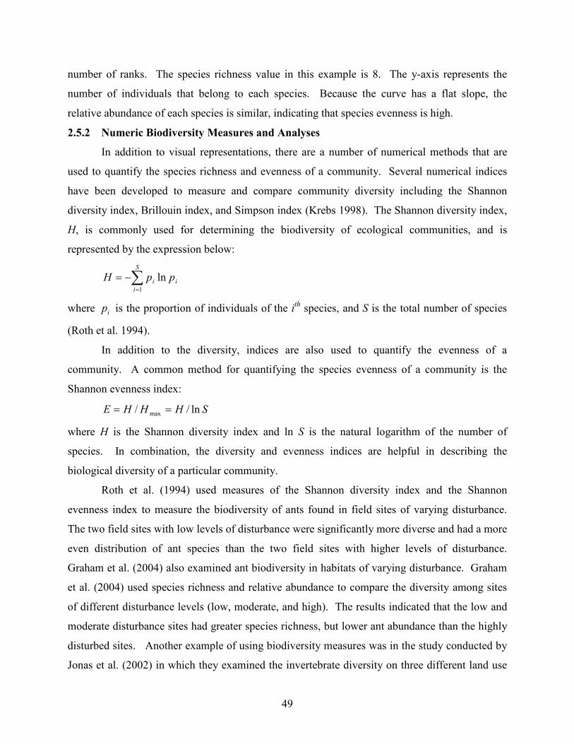
49

number of ranks. The species richness value in this example is 8. The y-axis represents the

number of individuals that belong to each species. Because the curve has a flat slope, the

relative abundance of each species is similar, indicating that species evenness is high.

2.5.2 Numeric Biodiversity Measures and Analyses

In addition to visual representations, there are a number of numerical methods that are

used to quantify the species richness and evenness of a community. Several numerical indices

have been developed to measure and compare community diversity including the Shannon

diversity index, Brillouin index, and Simpson index (Krebs 1998). The Shannon diversity index,

H, is commonly used for determining the biodiversity of ecological communities, and is

represented by the expression below:

∑=

−=S

i

ii ppH1

ln

where ip is the proportion of individuals of the ith species, and S is the total number of species

(Roth et al. 1994).

In addition to the diversity, indices are also used to quantify the evenness of a

community. A common method for quantifying the species evenness of a community is the

Shannon evenness index:

SHHHE ln// max ==

where H is the Shannon diversity index and ln S is the natural logarithm of the number of

species. In combination, the diversity and evenness indices are helpful in describing the

biological diversity of a particular community.

Roth et al. (1994) used measures of the Shannon diversity index and the Shannon

evenness index to measure the biodiversity of ants found in field sites of varying disturbance.

The two field sites with low levels of disturbance were significantly more diverse and had a more

even distribution of ant species than the two field sites with higher levels of disturbance.

Graham et al. (2004) also examined ant biodiversity in habitats of varying disturbance. Graham

et al. (2004) used species richness and relative abundance to compare the diversity among sites

of different disturbance levels (low, moderate, and high). The results indicated that the low and

moderate disturbance sites had greater species richness, but lower ant abundance than the highly

disturbed sites. Another example of using biodiversity measures was in the study conducted by

Jonas et al. (2002) in which they examined the invertebrate diversity on three different land use

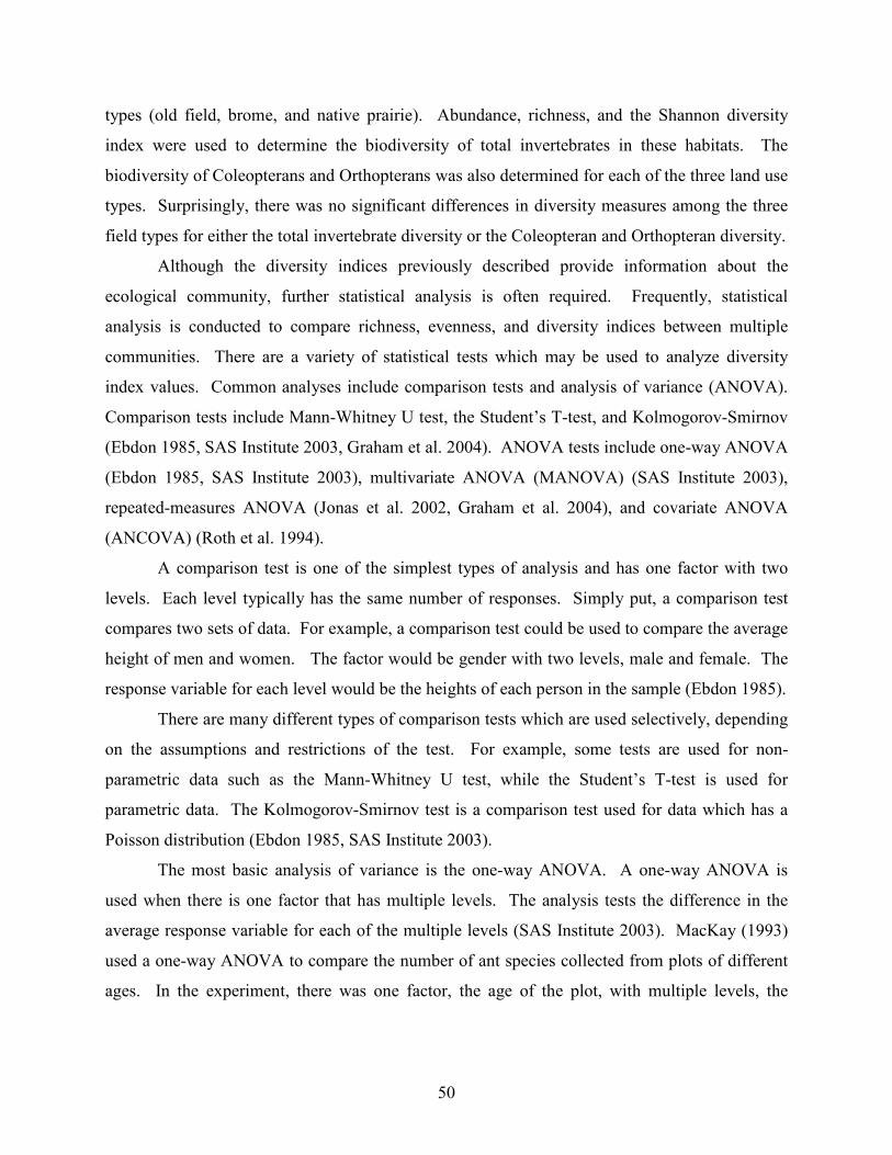
50

types (old field, brome, and native prairie). Abundance, richness, and the Shannon diversity

index were used to determine the biodiversity of total invertebrates in these habitats. The

biodiversity of Coleopterans and Orthopterans was also determined for each of the three land use

types. Surprisingly, there was no significant differences in diversity measures among the three

field types for either the total invertebrate diversity or the Coleopteran and Orthopteran diversity.

Although the diversity indices previously described provide information about the

ecological community, further statistical analysis is often required. Frequently, statistical

analysis is conducted to compare richness, evenness, and diversity indices between multiple

communities. There are a variety of statistical tests which may be used to analyze diversity

index values. Common analyses include comparison tests and analysis of variance (ANOVA).

Comparison tests include Mann-Whitney U test, the Student’s T-test, and Kolmogorov-Smirnov

(Ebdon 1985, SAS Institute 2003, Graham et al. 2004). ANOVA tests include one-way ANOVA

(Ebdon 1985, SAS Institute 2003), multivariate ANOVA (MANOVA) (SAS Institute 2003),

repeated-measures ANOVA (Jonas et al. 2002, Graham et al. 2004), and covariate ANOVA

(ANCOVA) (Roth et al. 1994).

A comparison test is one of the simplest types of analysis and has one factor with two

levels. Each level typically has the same number of responses. Simply put, a comparison test

compares two sets of data. For example, a comparison test could be used to compare the average

height of men and women. The factor would be gender with two levels, male and female. The

response variable for each level would be the heights of each person in the sample (Ebdon 1985).

There are many different types of comparison tests which are used selectively, depending

on the assumptions and restrictions of the test. For example, some tests are used for non-

parametric data such as the Mann-Whitney U test, while the Student’s T-test is used for

parametric data. The Kolmogorov-Smirnov test is a comparison test used for data which has a

Poisson distribution (Ebdon 1985, SAS Institute 2003).

The most basic analysis of variance is the one-way ANOVA. A one-way ANOVA is

used when there is one factor that has multiple levels. The analysis tests the difference in the

average response variable for each of the multiple levels (SAS Institute 2003). MacKay (1993)

used a one-way ANOVA to compare the number of ant species collected from plots of different

ages. In the experiment, there was one factor, the age of the plot, with multiple levels, the

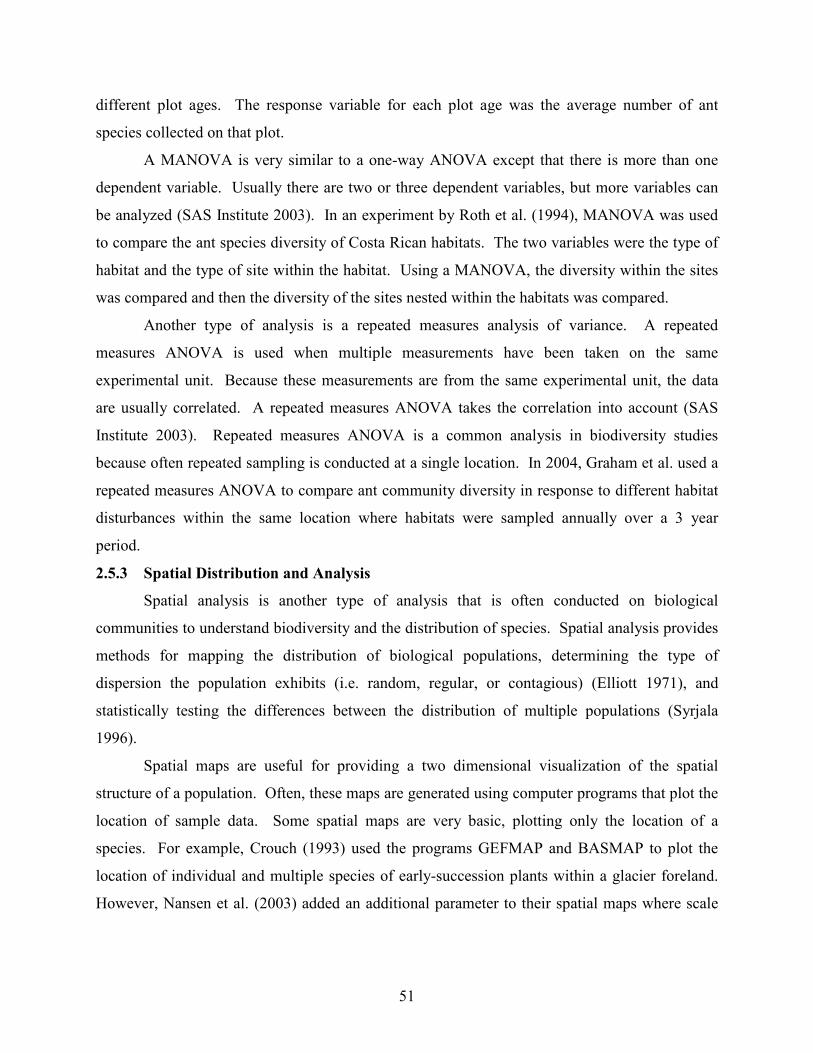
51

different plot ages. The response variable for each plot age was the average number of ant

species collected on that plot.

A MANOVA is very similar to a one-way ANOVA except that there is more than one

dependent variable. Usually there are two or three dependent variables, but more variables can

be analyzed (SAS Institute 2003). In an experiment by Roth et al. (1994), MANOVA was used

to compare the ant species diversity of Costa Rican habitats. The two variables were the type of

habitat and the type of site within the habitat. Using a MANOVA, the diversity within the sites

was compared and then the diversity of the sites nested within the habitats was compared.

Another type of analysis is a repeated measures analysis of variance. A repeated

measures ANOVA is used when multiple measurements have been taken on the same

experimental unit. Because these measurements are from the same experimental unit, the data

are usually correlated. A repeated measures ANOVA takes the correlation into account (SAS

Institute 2003). Repeated measures ANOVA is a common analysis in biodiversity studies

because often repeated sampling is conducted at a single location. In 2004, Graham et al. used a

repeated measures ANOVA to compare ant community diversity in response to different habitat

disturbances within the same location where habitats were sampled annually over a 3 year

period.

2.5.3 Spatial Distribution and Analysis

Spatial analysis is another type of analysis that is often conducted on biological

communities to understand biodiversity and the distribution of species. Spatial analysis provides

methods for mapping the distribution of biological populations, determining the type of

dispersion the population exhibits (i.e. random, regular, or contagious) (Elliott 1971), and

statistically testing the differences between the distribution of multiple populations (Syrjala

1996).

Spatial maps are useful for providing a two dimensional visualization of the spatial

structure of a population. Often, these maps are generated using computer programs that plot the

location of sample data. Some spatial maps are very basic, plotting only the location of a

species. For example, Crouch (1993) used the programs GEFMAP and BASMAP to plot the

location of individual and multiple species of early-succession plants within a glacier foreland.

However, Nansen et al. (2003) added an additional parameter to their spatial maps where scale

52

size dots were used to represent not only the location of Tenebrionid beetles, but the size of the

dot also represented the number of beetles collected at that location.

Another widely used mapping style for illustrating the abundance and location of a

particular species is contour mapping. Contour maps interpolate the expected population for an

entire area based on abundance data at individual locations within the area. Contour lines are

then constructed to differentiate between abundance values. The area between two contour lines

represents a uniform abundance (i.e. the abundance at any point between the two contour lines is

the same). The resulting map provides an extremely effective aid for visualizing the spatial

distribution of the target population (Thomas et al. 2001). Contour mapping programs include

Surfer (Golden Software, Golden, CO), GS+ (Gamma Design Software, Plainwell, MI), and

ArcGIS (Environmental Systems Research Institute, Redlands, CA).

Contour maps are commonly used in pest management programs to plot the location of

pests (Nansen et al. 2003). However, contour maps have some limitations and do not always

produce accurate contours due to limitation in the interpolating methodology. Nansen et al.

(2003) tested contour map population estimates against actual trap catches for Tenebrionid

beetles and found that the contours were inaccurate. Nansen et al. (2003) contributed the error to

having a small data set (N < 50) and the spatial distribution of the beetle populations (the beetle

populations were arranged in a random spatial structure). Nansen et al. (2003) concluded that

contour maps were an excellent tool but had limitations regarding the type of data that can be

analyzed.

The spatial dispersion of a population can be estimated by mapping the location of the

individuals. The spatial dispersion of a population is based on the distribution of the individuals

of the population (Elliott 1971). The distribution of the individuals is categorized as random,

regular, or contagious. A random distribution indicates that you have an equal chance of

encountering an individual anywhere within the sampling area. The location of one individual

does not have any affect on the location of the next. Therefore, some individuals may be

clumped into groups while others are spaced far apart. A regular distribution is characterized by

even spacing between all individuals. When the individuals are exactly the same distance apart

from each other, the distribution is described as perfectly regular. The third type of distribution

is the contagious distribution. Individuals are grouped together in this type of distribution. A

contagious distribution is also referred to as clumped or aggregated (Elliott 1971).

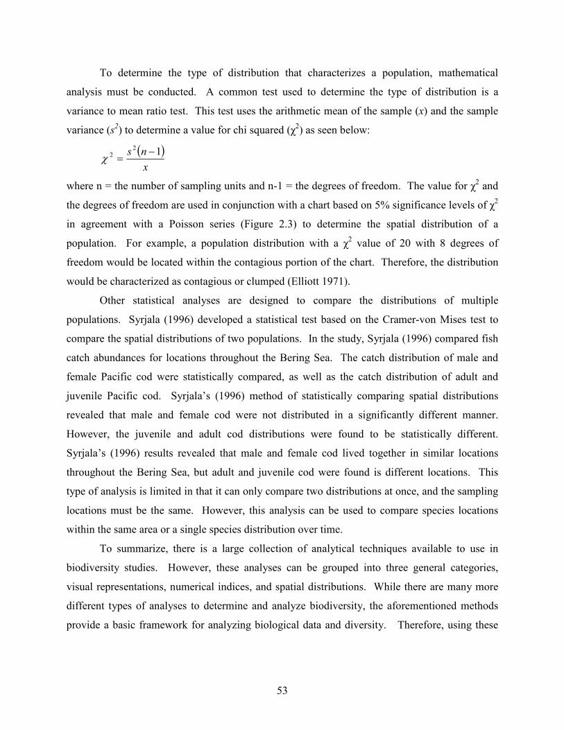
53

To determine the type of distribution that characterizes a population, mathematical

analysis must be conducted. A common test used to determine the type of distribution is a

variance to mean ratio test. This test uses the arithmetic mean of the sample (x) and the sample

variance (s2) to determine a value for chi squared (χ2) as seen below:

( )x

ns 122 −=χ

where n = the number of sampling units and n-1 = the degrees of freedom. The value for χ2 and

the degrees of freedom are used in conjunction with a chart based on 5% significance levels of χ2

in agreement with a Poisson series (Figure 2.3) to determine the spatial distribution of a

population. For example, a population distribution with a χ2 value of 20 with 8 degrees of

freedom would be located within the contagious portion of the chart. Therefore, the distribution

would be characterized as contagious or clumped (Elliott 1971).

Other statistical analyses are designed to compare the distributions of multiple

populations. Syrjala (1996) developed a statistical test based on the Cramer-von Mises test to

compare the spatial distributions of two populations. In the study, Syrjala (1996) compared fish

catch abundances for locations throughout the Bering Sea. The catch distribution of male and

female Pacific cod were statistically compared, as well as the catch distribution of adult and

juvenile Pacific cod. Syrjala’s (1996) method of statistically comparing spatial distributions

revealed that male and female cod were not distributed in a significantly different manner.

However, the juvenile and adult cod distributions were found to be statistically different.

Syrjala’s (1996) results revealed that male and female cod lived together in similar locations

throughout the Bering Sea, but adult and juvenile cod were found is different locations. This

type of analysis is limited in that it can only compare two distributions at once, and the sampling

locations must be the same. However, this analysis can be used to compare species locations

within the same area or a single species distribution over time.

To summarize, there is a large collection of analytical techniques available to use in

biodiversity studies. However, these analyses can be grouped into three general categories,

visual representations, numerical indices, and spatial distributions. While there are many more

different types of analyses to determine and analyze biodiversity, the aforementioned methods

provide a basic framework for analyzing biological data and diversity. Therefore, using these

54

methods we can begin to quantify biodiversity and changes in biodiversity over time and across

habitats.

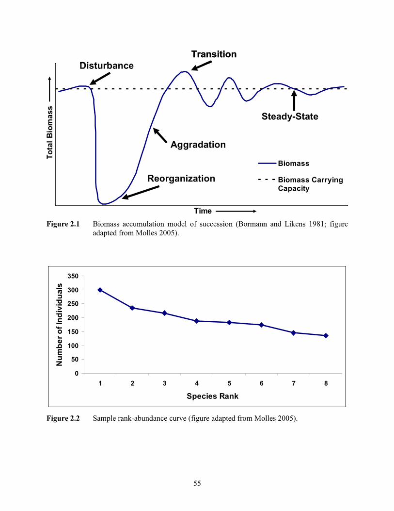
55

Time

Total Biomass

Biomass

Biomass CarryingCapacity

Disturbance

Reorganization

Aggradation

Transition

Steady-State

Time

Total Biomass

Biomass

Biomass CarryingCapacity

Disturbance

Reorganization

Aggradation

Transition

Steady-State

Figure 2.1 Biomass accumulation model of succession (Bormann and Likens 1981; figure adapted from Molles 2005).

0

50

100

150

200

250

300

350

1 2 3 4 5 6 7 8

Species Rank

Number of Individuals

Figure 2.2 Sample rank-abundance curve (figure adapted from Molles 2005).

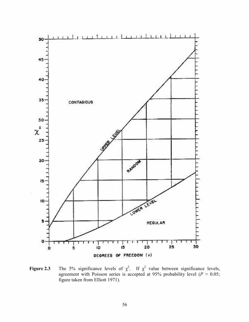
56

Figure 2.3 The 5% significance levels of χ2. If χ2 value between significance levels, agreement with Poisson series is accepted at 95% probability level (P > 0.05; figure taken from Elliott 1971).

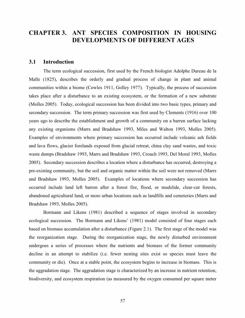
57

CHAPTER 3. ANT SPECIES COMPOSITION IN HOUSING

DEVELOPMENTS OF DIFFERENT AGES

3.1 Introduction

The term ecological succession, first used by the French biologist Adolphe Dureau de la

Malle (1825), describes the orderly and gradual process of change in plant and animal

communities within a biome (Cowles 1911, Golley 1977). Typically, the process of succession

takes place after a disturbance to an existing ecosystem, or the formation of a new substrate

(Molles 2005). Today, ecological succession has been divided into two basic types, primary and

secondary succession. The term primary succession was first used by Clements (1916) over 100

years ago to describe the establishment and growth of a community on a barren surface lacking

any existing organisms (Marrs and Bradshaw 1993, Miles and Walton 1993, Molles 2005).

Examples of environments where primary succession has occurred include volcanic ash fields

and lava flows, glacier forelands exposed from glacial retreat, china clay sand wastes, and toxic

waste dumps (Bradshaw 1993, Marrs and Bradshaw 1993, Crouch 1993, Del Moral 1993, Molles

2005). Secondary succession describes a location where a disturbance has occurred, destroying a

pre-existing community, but the soil and organic matter within the soil were not removed (Marrs

and Bradshaw 1993, Molles 2005). Examples of locations where secondary succession has

occurred include land left barren after a forest fire, flood, or mudslide, clear-cut forests,

abandoned agricultural land, or more urban locations such as landfills and cemeteries (Marrs and

Bradshaw 1993, Molles 2005).

Bormann and Likens (1981) described a sequence of stages involved in secondary

ecological succession. The Bormann and Likens’ (1981) model consisted of four stages each

based on biomass accumulation after a disturbance (Figure 2.1). The first stage of the model was

the reorganization stage. During the reorganization stage, the newly disturbed environment

undergoes a series of processes where the nutrients and biomass of the former community

decline in an attempt to stabilize (i.e. fewer nesting sites exist so species must leave the

community or die). Once at a stable point, the ecosystem begins to increase in biomass. This is

the aggradation stage. The aggradation stage is characterized by an increase in nutrient retention,

biodiversity, and ecosystem respiration (as measured by the oxygen consumed per square meter

58

per day). The aggradation stage continues until biomass accumulation reaches a peak. This peak

usually occurs when all the available resources of the ecosystem are being utilized and no further

biomass (i.e. animal or plant life) can be supported. At this point, the ecosystem enters the

transition phase. During the transition phase, species interactions begin to influence the species

composition of the environment leading to a minor decline in biomass. The final stage, known

as the steady-state phase, occurs when the community becomes stable and there are no further

major increases or decreases in biomass or diversity. In the steady-stage phase, the community

is referred to as a climax community and remains as such until another disturbance takes place

(Bormann and Likens 1981, Molles 2005).

Throughout the stages of succession, the environmental complexity of the community

increases (Molles 2005). This increase in environmental complexity results in an increase in the

biodiversity of the community because biodiversity is generally higher in more complex

environments. Biodiversity can be defined as the number of species coexisting within a

community and their relative abundance (Molles 2005).

While most studies on ecological succession focus on natural communities, urban

succession focuses on successional processes that take place in urban ecosystems. Urban

ecosystems vary in size and complexity, and therefore contain many different ecological niches.

Urban ecosystems include residential lawns and gardens, industrial sites, abandoned properties,

parks and play grounds, cemeteries, waste disposal sites, managed forests, fields, and bodies of

water (Nagle 1999). Unlike ecological succession, urban succession only occurs as the result of

a human disturbance which typically happens during the process of urbanization. During

urbanization, vegetation is removed and the soil is graded. This process leaves a barren substrate

where urban succession can occur. Plants and animals slowly reestablish in the disturbed

ecosystem, increasing the environmental complexity and thus, causing species diversity and

evenness to increase (Rebele 1994).

An excellent example of a location where humans have repeatedly impacted the

environment and the successional process is the island of Puerto Rico. Due to past agricultural

practices and present urbanization, broad scale human disturbances have become a characteristic

of Puerto Rican ecosystems (Aide et al. 2000, Chinea and Helmer 2003, Grau et al. 2003). Grau

et al. (2003) described Puerto Rico as a large scale ecological experiment of almost 1 million ha

that has been subjected to intense human disturbance for almost 100 years.

59

In the late 20th century, the economy of Puerto Rico underwent a major shift from

agriculture (coffee, sugarcane, and cattle) to an industrialized economy based on manufacturing

and services (Lopez et al. 2001, Grau et al. 2003, Helmer 2004). Prior to 1940, the Puerto Rican

economy was almost completely dependent on agriculture (Lopez et al. 2001). However, by

1996 the shift from an agrarian to an industrial economy resulted in the abandonment of

agricultural lands as people moved from rural areas to industrial and urban locations. As the

population migrated from rural farmlands to cities, rapid urban expansion occurred. Lopez et al.

(2001) found that urban areas covered nearly 15% of the island. In one case study, Thomlinson

and Rivera (2000) found that between 1936 and 1988, there was a 2,000% increase in urban

areas around the city of Luquillo. One end product of the rapid urban expansion has been the

construction of numerous housing developments. Thus, the resulting landscape of Puerto Rico

has changed from agricultural fields to a mosaic of housing developments of varying ages.

These housing developments and their resulting biological communities represent different

stages of urban succession (Lopez et al. 2001, Helmer 2004).

Throughout the numerous disturbances taking place on the island over the past century,

ants have remained one of the most prolific organisms in Puerto Rico. Levins et al. (1973)

determined that ants were the most abundant invertebrates on the island. The large number of

ant species and their high level of abundance have enticed many researchers to study the ant

fauna in Puerto Rico. In the past century, Wheeler (1908), Smith (1936), Levins et al. (1973),

and most recently, Torres and Snelling (1997) have attempted to catalogue all of the ant species

in Puerto Rico. In addition to cataloguing all ant species on the island, studies describing the ant

fauna at localized sites around the island have been conducted by Culver (1974), Lavinge (1977),

and Torres (1984a, 1984b).

However, despite the thorough documentation of the ants of Puerto Rico, little has been

done to categorize the species that occur in urban environments. Furthermore, the succession of

the Puerto Rican ant species complex within urban environments has not been examined.

Therefore, the primary purpose of this study was to determine the ant species composition in

Puerto Rican housing developments of different ages and to determine whether these

developments were representative of the biomass accumulation model described by Bormann

and Likens (1981). In addition, this study attempted to characterize the housing developments

by quantifying the ant species richness and abundance at each site. Rank-abundance curves were

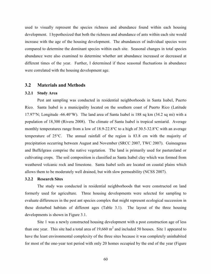
60

used to visually represent the species richness and abundance found within each housing

development. I hypothesized that both the richness and abundance of ants within each site would

increase with the age of the housing development. The abundances of individual species were

compared to determine the dominant species within each site. Seasonal changes in total species

abundance were also examined to determine whether ant abundance increased or decreased at

different times of the year. Further, I determined if these seasonal fluctuations in abundance

were correlated with the housing development age.

3.2 Materials and Methods

3.2.1 Study Area

Pest ant sampling was conducted in residential neighborhoods in Santa Isabel, Puerto

Rico. Santa Isabel is a municipality located on the southern coast of Puerto Rico (Latitude

17.97°N; Longitude -66.40°W). The land area of Santa Isabel is 188 sq km (34.2 sq mi) with a

population of 18,300 (Rivera 2008). The climate of Santa Isabel is tropical semiarid. Average

monthly temperatures range from a low of 18.9-22.8°C to a high of 30.5-32.8°C with an average

temperature of 25°C. The annual rainfall of the region is 83.8 cm with the majority of

precipitation occurring between August and November (SRCC 2007, TWC 2007). Guineagrass

and Buffelgrass comprise the native vegetation. The land is primarily used for pastureland or

cultivating crops. The soil composition is classified as Santa Isabel clay which was formed from

weathered volcanic rock and limestone. Santa Isabel soils are located on coastal plains which

allows them to be moderately well drained, but with slow permeability (NCSS 2007).

3.2.2 Research Sites

The study was conducted in residential neighborhoods that were constructed on land

formerly used for agriculture. Three housing developments were selected for sampling to

evaluate differences in the pest ant species complex that might represent ecological succession in

these disturbed habitats of different ages (Table 3.1). The layout of the three housing

developments is shown in Figure 3.1.

Site 1 was a newly constructed housing development with a post construction age of less

than one year. This site had a total area of 19,660 m2 and included 50 houses. Site 1 appeared to

have the least environmental complexity of the three sites because it was completely uninhabited

for most of the one-year test period with only 20 homes occupied by the end of the year (Figure

61

3.2A). The houses themselves were structurally simple and of uniform design. Because the

houses were empty, the yards were unkempt, resulting in ~2 m weed growth by the end of the

test. Site 1 was bordered on the south side by a working construction site. On the west side was

a mulched playground. Site 1 had a four-lane highway on the northern border and another

residential neighborhood on its eastern side.

A four year old housing development was used as the second sampling site (Site 2). Site

2 was the residential neighborhood to the east of Site 1 and consisted of 77 houses in an area of

26,337 m2. Nearly all houses in Site 2 were inhabited resulting in a more complex environment

than in Site 1 (Figure 3.2B). Most of the houses had been customized with the addition of

exterior walls, closed garages, and porches. The yards contained small trees and shrubs,

fountains, and other landscaping features. Because Site 2 was inhabited, trash containers were

also present. The plastic trash containers were placed into holes that had been dug in the yard so

that the lids were at grade level. On the north side, Site 2 was bordered by the same four-lane

highway that bordered Site 1. Pastureland was on the east side, and a housing development of

similar age bordered Site 2 on the southern side.

The third site (Site 3) was approximately eight years old. The neighborhood had a total

area of 55,193 m2 and contained 157 houses. Like Site 2, Site 3 was fully inhabited, resulting in

an environmentally complex habitat (Figure 3.2C). Nearly all the houses were customized with

unique construction features and yards that ranged in complexity from bare earth to elaborate

landscaping with mature trees and shrubs. Site 3 was bordered by the four-lane highway on the

south side and abandoned pastureland on the other three sides.

3.2.3 Sampling Procedure

At the initiation of the study, I contacted all the homeowners within each site and

requested permission to sample. Based on the location of the houses where permission was

granted, 30 houses were selected for sampling to achieve a representative sample distribution

over the entire study site.

Food based baits were used to collect ant samples. The baiting method consisted of

cotton rope (5.6 mm Wellington Medium Load Braided Cotton Multi-Purpose Clothesline;

Wellington Cordage, Madison, GA) cut into ~3.8 cm segments. Rope segments were soaked in

one of two food attractants; a 25% sucrose solution (Kroger Granulated Sugar; Kroger Co.,

Cincinnati, OH) or peanut oil (LouAna Peanut Oil; Ventura Foods, Brea, CA). After soaking,

62

excess sugar water or peanut oil was pressed from the rope segments and a single segment was

inserted into a glass vial with a screw cap (2 dram; Bioquip, Rancho Dominguez, CA). A pair of

baited vials, one sugar and one peanut oil, was then placed at three locations around the front

exterior of each sample house. The three sampling locations on each property were located at

the bottom corner of the front door, the side corner of the house, and the corner adjacent to the

garage (Figure 3.3). The baits were left at the sampling locations for one hour and then

collected. Upon collection of the sample vials, the caps were placed on the vials to capture any

ants feeding on the baits. The vials were placed into boxes marked with corresponding location

data. After all the vials at a site had been collected, isopropyl alcohol (70%; readily available in

Puerto Rico), was added to each vial to kill and preserve the collected ants.

The baiting regimen was conducted twice a day over a two day period at each site

between 7:00 and 10:00 am, and between 4:00 and 7:00 pm depending on seasonal daylight

hours. A total of eight two-day sampling trips were conducted at approximately six week

intervals so that the ants were sampled two times per season (Appendix A). At the end of each

sampling trip, all samples were transported back to the Dodson Urban Pest Management

Laboratory (DUPML) at Virginia Tech. In the laboratory, the ants were removed from the glass

vials and placed into clean plastic vials (7 ml HDPE Scintillation Vials; Fisher Scientific,

Waltham, MA) containing isopropyl alcohol (70%). The ant species in each vial were identified,

and the number of individuals in each species was recorded.

Pitfall traps were also installed during the August, October, November, and January

sampling periods. Between three and five pitfall traps were placed around the periphery of each

site, and in open areas within the site. The purpose of the pitfall traps was to monitor for ant

species that were either not attracted to the baits, or that lived in areas adjacent to the residential

sites. Pitfall traps were constructed by placing clear plastic cups (266 ml; Club cups, Matosantos

Commercial Corporation, San Juan, Puerto Rico) inside holes in the soil. Cups were filled two

thirds full with water and a drop of dishwashing detergent (Dawn; Procter & Gamble, Cincinnati,

OH). Traps were covered with a 15 x 15 x 0.3175 cm hardboard panel (Signature S2S High

Performance Panel, Decorative Panels International, Toledo, OH) with nails driven into each

corner. The nails were inserted into the ground over the cup leaving approximately a 2 cm space

between the cover and the cup. The cover prevented larger animals from accessing the cup and

also reduced water evaporation. Pitfall traps were left for 48 hours and then collected. All the

63

contents of the pitfall trap were transferred into a plastic bottle (125 ml HDPE Narrow-Mouth

Sample Bottles; Nalge Nunc International, Rochester, NY) for transportation back to the

DUPML. At the laboratory, the contents of the pitfalls traps were examined and any ants found

were collected and stored in isopropyl alcohol (70%). All ant species from pitfall traps were

identified and quantified.

All ant samples were identified to genus using Holldobler and Wilson (1990) and Bolton

(1994). Snelling and Torres’ (unpublished data) manuscript, The Ants of Puerto Rico, was used

to identify ants to the species level. Taxonomic images from AntWeb (CAS 2008) and Discover

Life (Lim and Pickering 2008) were also used to assist the identification process. Species

identifications were verified by Matthew Buffington, Systematic Entomology Laboratory,

USDA. Specimens were deposited in the Virginia Tech Insect Collection.

Weather data were recorded at a local weather station at Mycogen Seeds Research

Corporation in Santa Isabel, PR. The mean daily temperature during each sampling period fell

within the minimum and maximum mean temperature boundaries. Mean daily temperatures

ranged between 23.7°C (March) and 28.3°C (May). The sites experienced precipitation during

all sampling periods except in May and January. However, the only sampling trips during which

there were more than 1.0 mm of rainfall were in April (7.37 mm), June (13.46 mm), and October

(4.57 mm). Relative humidity was always high during the sampling trips, ranging from 76%-

100% (Table 3.2).

3.2.4 Species Composition

The number of species and individuals per species in each sample was recorded. A list of

the collected species from bait and pitfall traps was compiled to determine the pest ant species

complex within the Santa Isabel housing developments. From the species list, occurrence

diagrams were created to visually represent which species were present or absent within each site

(Tabor et al. 2004). Species richness, S (Roth et al. 1994), and relative abundance (the number

of individuals belonging to a single species divided by the total number of individuals from all

species; Molles 2005), p, were determined for each site by combining bait and pitfall trap data.

Rank-abundance curves were generated to compare species diversity between the sites (Molles

2005). Relative abundance pie charts were also generated from the combined sampling data to

determine the dominant species within each site.

64

Species richness and abundance data from bait samples were also recorded by month and

used to generate occurrence diagrams. The occurrence diagrams indicated which species were

collected during each sampling period. Bait sample data were also used to examine seasonal

changes in ant composition.

3.3 Results

3.3.1 Species Composition

A total of 8,679 samples (8,640 bait samples and 39 pitfall samples) were collected from

the three housing developments. Those samples yielded 246,972 individual ants representing 25

different species (Table 3.3). Bait samples yielded 243,252 individual ants from 19 species

(Appendix B) and pitfall traps yielded 3,720 individual ants representing 20 species (Appendix

C). Sixteen genera were collected representing five Neotropical subfamilies. Of the five

subfamilies, 16 species were from Myrmicinae, three species each were from Dolichoderinae and

Formicinae, two species were from Ponerinae, and one species was from Pseudomyrmecinae.

Out of the 25 species collected, five were collected only in the bait samples (Tapinoma rasenum,

Dorymyrmex antillana, Brachymyrmex sp. 2, Pheidole megacephala, and Wasmannia

auropunctata) and six species were collected only in pitfall traps (Crematogaster steinheili,

Cyphomyrmex minutus, Solenopsis pygmaea B, Tetramorium simillimum, Hypoponera

punctatissima, and Pseudomyrmex simplex) (Table 3.3).

The number of species which were collected at each site increased with the age of the

housing development. The fewest number of species were collected from the one-year-old

housing development (Site 1; 14 species), followed by the four-year-old housing development

(Site 2; 20 species). The eight-year-old housing development (Site 3) had the greatest number of

species (21 species) (Figure 3.4).

The total ant biomass collected from each site also differed depending on the age of the

housing development. These changes in biomass indicated that the sites represented different

stages of succession. Of the 246,278 ants collected, 23.8% (58,537 ants) were collected from

Site 1. The greatest percentage of ants, 40.3% (99,273 ants) were collected from Site 2, followed

by Site 3 with 35.9% (88,468 ants) of the total number of ants collected (Figure 3.4).

Rank-abundance curves were used to compare diversity within the different habitats.

Figure 3.5 is a rank-abundance diagram that was constructed using both the species richness and

65

abundance data collected from all samples at each site. Site 1 had the least diversity and is

represented by the fewest ranks (14) on the x-axis (Figure 3.5). The rank-abundance curves for

Sites 2 and 3 were very similar to each other. However, the curve for Site 3 had one more rank

than Site 2 indicating that Site 3 had greater species richness. The abundance values in Site 3

(total number of ants collected), for each species ranked from 1-12, were more equivalent to each

other than those in Sites 1 and 2 indicating that Site 3 also had greater evenness.

3.3.2 Species Abundance

The abundance of each individual species was compared to determine the dominant

species within each site (Figure 3.6). In Site 1, the dominant species was S. invicta, which

accounted for 57.33% of all the ants collected. Brachymyrmex sp. 1 and P. moerens were also

determined to be dominant species with 19.85% and 11.56% relative abundances, respectively.

S. invicta was also the dominant species in Site 2, representing 43.31% of the ants collected.

However, the second and third most abundant species in Site 2 were M. destructor (20.76%) and

P. fallax (14.35%). S. invicta was also the dominant species in Site 3 with a relative abundance

of 46.37%. P. fallax was the second most abundant species (13.05%). However, nine other

species had a relative abundance between 1 and 10% indicating a high level of species evenness

in Site 3.

3.3.3 Species Collected Using Baits

Data from the bait samples were used to generate occurrence diagrams to indicate which

species were collected during each sampling period (Table 3.4). Ten out of the 19 total species

were collected at all three sites at least once during the year-long test period. Three species,

Brachymyrmex sp. 1, Pheidole moerens, and Solenopsis invicta, were collected during every

sampling trip (8 total trips) in all three sites. One additional species, S. globularia, was collected

during every sampling trip, but only in Site 1. Six species were collected in Site 2 during every

sampling period; T. melanocephalum, P. longicornis, M. destructor, P. fallax, P. megacephala,

and O. ruginodis. Five species were collected in Site 3 during every sampling period; T.

melanocephalum, P. longicornis, P. fallax, C. emeryi, and P. subarmata.

The number of species (species richness) that were collected in a single sampling period

ranged from six to 15 depending on the age of the housing development and the month (Figure

3.7). However, the species richness of each site remained relatively constant throughout the

year. Interestingly, the greatest species richness within each site occurred in November (10

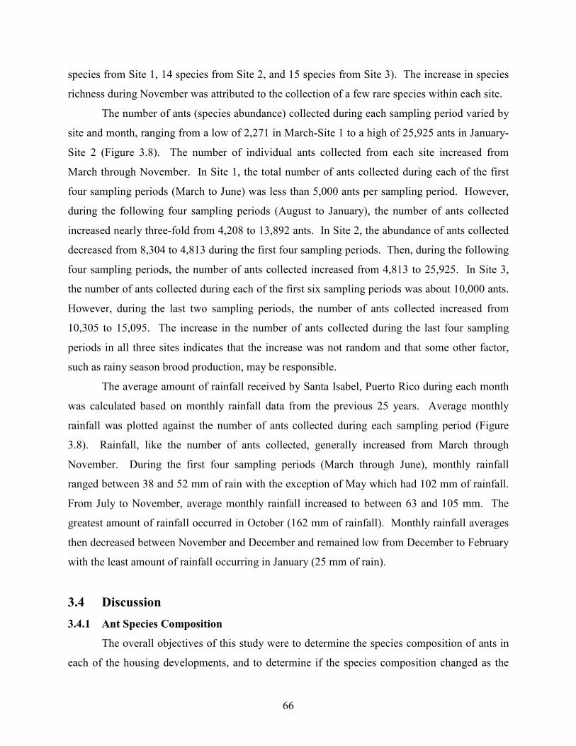
66

species from Site 1, 14 species from Site 2, and 15 species from Site 3). The increase in species

richness during November was attributed to the collection of a few rare species within each site.

The number of ants (species abundance) collected during each sampling period varied by

site and month, ranging from a low of 2,271 in March-Site 1 to a high of 25,925 ants in January-

Site 2 (Figure 3.8). The number of individual ants collected from each site increased from

March through November. In Site 1, the total number of ants collected during each of the first

four sampling periods (March to June) was less than 5,000 ants per sampling period. However,

during the following four sampling periods (August to January), the number of ants collected

increased nearly three-fold from 4,208 to 13,892 ants. In Site 2, the abundance of ants collected

decreased from 8,304 to 4,813 during the first four sampling periods. Then, during the following

four sampling periods, the number of ants collected increased from 4,813 to 25,925. In Site 3,

the number of ants collected during each of the first six sampling periods was about 10,000 ants.

However, during the last two sampling periods, the number of ants collected increased from

10,305 to 15,095. The increase in the number of ants collected during the last four sampling

periods in all three sites indicates that the increase was not random and that some other factor,

such as rainy season brood production, may be responsible.

The average amount of rainfall received by Santa Isabel, Puerto Rico during each month

was calculated based on monthly rainfall data from the previous 25 years. Average monthly

rainfall was plotted against the number of ants collected during each sampling period (Figure

3.8). Rainfall, like the number of ants collected, generally increased from March through

November. During the first four sampling periods (March through June), monthly rainfall

ranged between 38 and 52 mm of rain with the exception of May which had 102 mm of rainfall.

From July to November, average monthly rainfall increased to between 63 and 105 mm. The

greatest amount of rainfall occurred in October (162 mm of rainfall). Monthly rainfall averages

then decreased between November and December and remained low from December to February

with the least amount of rainfall occurring in January (25 mm of rain).

3.4 Discussion

3.4.1 Ant Species Composition

The overall objectives of this study were to determine the species composition of ants in

each of the housing developments, and to determine if the species composition changed as the

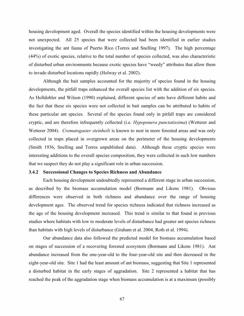
67

housing development aged. Overall the species identified within the housing developments were

not unexpected. All 25 species that were collected had been identified in earlier studies

investigating the ant fauna of Puerto Rico (Torres and Snelling 1997). The high percentage

(44%) of exotic species, relative to the total number of species collected, was also characteristic

of disturbed urban environments because exotic species have “weedy” attributes that allow them

to invade disturbed locations rapidly (Holway et al. 2002).

Although the bait samples accounted for the majority of species found in the housing

developments, the pitfall traps enhanced the overall species list with the addition of six species.

As Holldobler and Wilson (1990) explained, different species of ants have different habits and

the fact that these six species were not collected in bait samples can be attributed to habits of

these particular ant species. Several of the species found only in pitfall traps are considered

cryptic, and are therefore infrequently collected (i.e. Hypoponera punctatissima) (Wetterer and

Wetterer 2004). Crematogaster steinheili is known to nest in more forested areas and was only

collected in traps placed in overgrown areas on the perimeter of the housing developments

(Smith 1936, Snelling and Torres unpublished data). Although these cryptic species were

interesting additions to the overall species composition, they were collected in such low numbers

that we suspect they do not play a significant role in urban succession.

3.4.2 Successional Changes to Species Richness and Abundance

Each housing development undoubtedly represented a different stage in urban succession,

as described by the biomass accumulation model (Bormann and Likens 1981). Obvious

differences were observed in both richness and abundance over the range of housing

development ages. The observed trend for species richness indicated that richness increased as

the age of the housing development increased. This trend is similar to that found in previous

studies where habitats with low to moderate levels of disturbance had greater ant species richness

than habitats with high levels of disturbance (Graham et al. 2004, Roth et al. 1994).

Our abundance data also followed the predicted model for biomass accumulation based

on stages of succession of a recovering forested ecosystem (Bormann and Likens 1981). Ant

abundance increased from the one-year-old to the four-year-old site and then decreased in the

eight-year-old site. Site 1 had the least amount of ant biomass, suggesting that Site 1 represented

a disturbed habitat in the early stages of aggradation. Site 2 represented a habitat that has

reached the peak of the aggradation stage when biomass accumulation is at a maximum (possibly

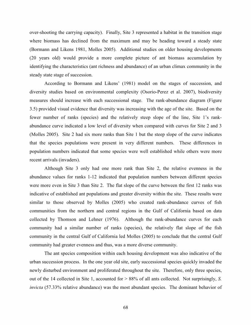
68

over-shooting the carrying capacity). Finally, Site 3 represented a habitat in the transition stage

where biomass has declined from the maximum and may be heading toward a steady state

(Bormann and Likens 1981, Molles 2005). Additional studies on older housing developments

(20 years old) would provide a more complete picture of ant biomass accumulation by

identifying the characteristics (ant richness and abundance) of an urban climax community in the

steady state stage of succession.

According to Bormann and Likens’ (1981) model on the stages of succession, and

diversity studies based on environmental complexity (Osorio-Perez et al. 2007), biodiversity

measures should increase with each successional stage. The rank-abundance diagram (Figure

3.5) provided visual evidence that diversity was increasing with the age of the site. Based on the

fewer number of ranks (species) and the relatively steep slope of the line, Site 1’s rank-

abundance curve indicated a low level of diversity when compared with curves for Site 2 and 3

(Molles 2005). Site 2 had six more ranks than Site 1 but the steep slope of the curve indicates

that the species populations were present in very different numbers. These differences in

population numbers indicated that some species were well established while others were more

recent arrivals (invaders).

Although Site 3 only had one more rank than Site 2, the relative evenness in the

abundance values for ranks 1-12 indicated that population numbers between different species

were more even in Site 3 than Site 2. The flat slope of the curve between the first 12 ranks was

indicative of established ant populations and greater diversity within the site. These results were

similar to those observed by Molles (2005) who created rank-abundance curves of fish

communities from the northern and central regions in the Gulf of California based on data

collected by Thomson and Lehner (1976). Although the rank-abundance curves for each

community had a similar number of ranks (species), the relatively flat slope of the fish

community in the central Gulf of California led Molles (2005) to conclude that the central Gulf

community had greater evenness and thus, was a more diverse community.

The ant species composition within each housing development was also indicative of the

urban succession process. In the one year old site, early successional species quickly invaded the

newly disturbed environment and proliferated throughout the site. Therefore, only three species,

out of the 14 collected in Site 1, accounted for > 88% of all ants collected. Not surprisingly, S.

invicta (57.33% relative abundance) was the most abundant species. The dominant behavior of

69

S. invicta has been well studied and this species is well known for its ability to rapidly invade

and establish in newly disturbed environments (Holway et al. 2002). The second most abundant

species in Site 1 was Brachymyrmex sp. 1 (19.85% relative abundance). In general, little is

known about this genus. Brachymyrmex biology and species identification delineations are not

well known (Deyrup et al. 2000, Snelling and Torres unpublished data, MacGown et al. 2007).

However, MacGown et al. (2007) recently identified one species, B. patagonicus, as an emerging

pest species in the southeastern United States. Although no records of B. patagonicus exist from

Puerto Rico, our findings indicate that Brachymyrmex sp. 1 is able to quickly invade newly

disturbed environments as an early successional species and may also be considered a nuisance

pest. The third most abundant species in Site 1 was Pheidole moerens. P. moerens has been

found in both urban and wooded locations throughout Puerto Rico and is thought to be a native

species (Deyrup et al. 2000, Snelling and Torres unpublished data).

Site 2 (the four year old site) represented the transition stage of urban succession and, as

expected, had a greater number of species than Site 1 (Osorio-Perez et al. 2007, MacKay 1993,

Majer 1983). Several species represented mid-successional species that are slower to invade

disturbed habitats, but are able to compete with the species that are already present. Similar

studies by Haering and Fox (1987) and Majer (1983) also identified mid-successional ant species

in rehabilitated mining sites. These species were not founding species, but were able to invade

disturbed habitats that were already occupied, and in some cases, displaced earlier successional

species. Although six more species were collected in Site 2 than Site 1, three dominant species

still constituted the majority (> 75%) of the ants collected. Not surprisingly, S. invicta remained

the most abundant species collected (41.31% relative abundance). Not only is S. invicta well

known for its rapid dispersal capabilities, but S. invicta has been identified as an aggressive

species that is not easily displaced once it is established (Holway et al. 2002, Tsutsui and Suarez

2003).

The second most abundant species in Site 2 was Monomorium destructor (20.76%

relative abundance). This species was not collected in Site 1. M. destructor’s apparent

dominance in Site 2, and its absence in Site 1, indicates that this species is not typically a

founding species in newly disturbed habitats. Although it is not a founding species, M.

destructor appears to be able to proliferate successfully in disturbed habitats and compete with

other established species. Smith (1965) reported that M. destructor formed large polygyne

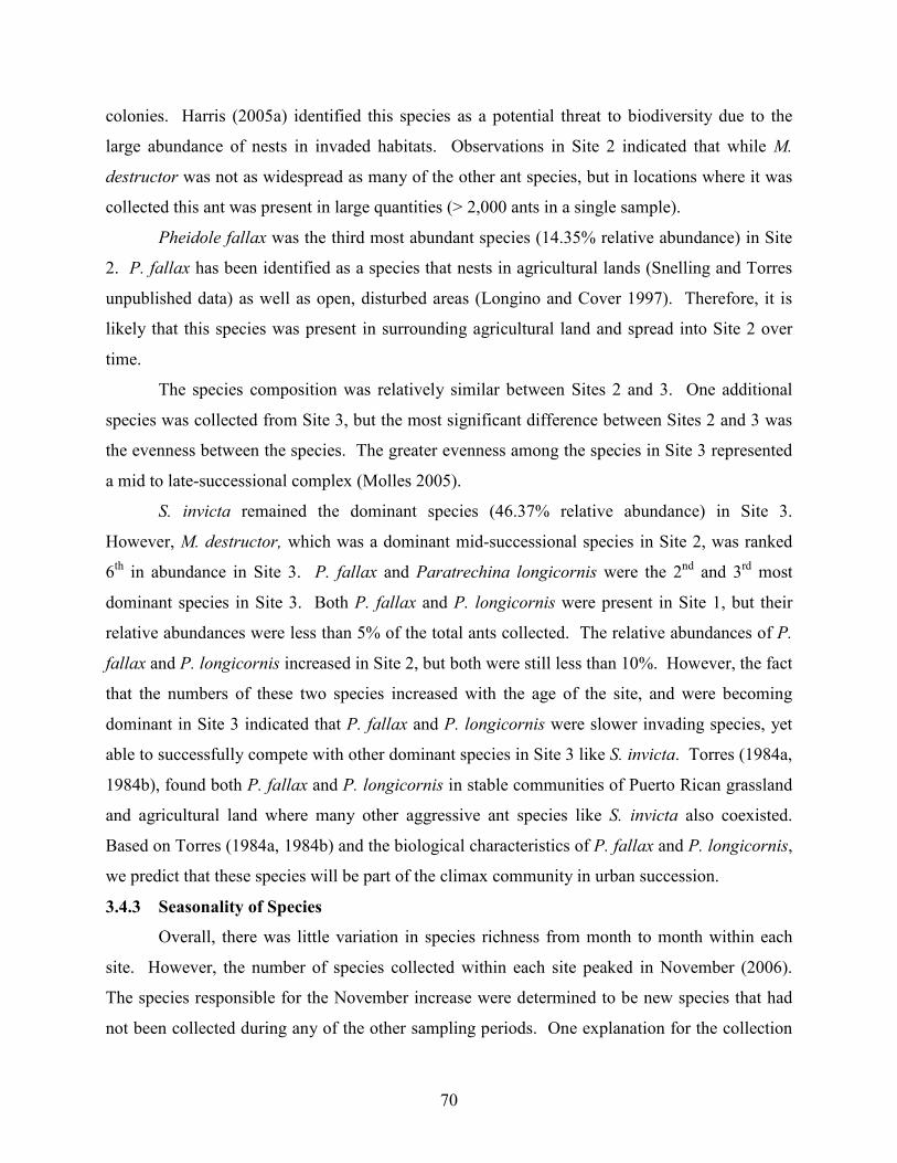
70

colonies. Harris (2005a) identified this species as a potential threat to biodiversity due to the

large abundance of nests in invaded habitats. Observations in Site 2 indicated that while M.

destructor was not as widespread as many of the other ant species, but in locations where it was

collected this ant was present in large quantities (> 2,000 ants in a single sample).

Pheidole fallax was the third most abundant species (14.35% relative abundance) in Site

2. P. fallax has been identified as a species that nests in agricultural lands (Snelling and Torres

unpublished data) as well as open, disturbed areas (Longino and Cover 1997). Therefore, it is

likely that this species was present in surrounding agricultural land and spread into Site 2 over

time.

The species composition was relatively similar between Sites 2 and 3. One additional

species was collected from Site 3, but the most significant difference between Sites 2 and 3 was

the evenness between the species. The greater evenness among the species in Site 3 represented

a mid to late-successional complex (Molles 2005).

S. invicta remained the dominant species (46.37% relative abundance) in Site 3.

However, M. destructor, which was a dominant mid-successional species in Site 2, was ranked

6th in abundance in Site 3. P. fallax and Paratrechina longicornis were the 2nd and 3rd most

dominant species in Site 3. Both P. fallax and P. longicornis were present in Site 1, but their

relative abundances were less than 5% of the total ants collected. The relative abundances of P.

fallax and P. longicornis increased in Site 2, but both were still less than 10%. However, the fact

that the numbers of these two species increased with the age of the site, and were becoming

dominant in Site 3 indicated that P. fallax and P. longicornis were slower invading species, yet

able to successfully compete with other dominant species in Site 3 like S. invicta. Torres (1984a,

1984b), found both P. fallax and P. longicornis in stable communities of Puerto Rican grassland

and agricultural land where many other aggressive ant species like S. invicta also coexisted.

Based on Torres (1984a, 1984b) and the biological characteristics of P. fallax and P. longicornis,

we predict that these species will be part of the climax community in urban succession.

3.4.3 Seasonality of Species

Overall, there was little variation in species richness from month to month within each

site. However, the number of species collected within each site peaked in November (2006).

The species responsible for the November increase were determined to be new species that had

not been collected during any of the other sampling periods. One explanation for the collection

71

of new species during the November sampling period was that the abundances of all species

collected in November were extremely high. Similar studies on the seasonal changes in richness

and abundance of ant communities arrived at the same conclusion. For example, in the Republic

of Panama, Levings (1983) found that more species of ants were collected when ant abundance

was at a seasonal peak. Therefore, we suggest that the new species found in our study were more

easily collected in November, when all ant populations were at their peak.

Unlike species richness, the total number of ants collected during each sampling period

steadily increased throughout the year (March 2006 to January 2007). Seasonal increases in ant

abundance have been well documented in many studies (Levings 1983, Retana and Cerda 2000,

Philpott et al. 2006). The magnitude of increasing ant abundance was the most significant in Site

2. Comparatively, more ants were present at the beginning of the year in Site 2 than in Sites 1 or

3. The greater amount of initial biomass in Site 2 enabled the ants to reach a maximum

abundance greater than either of the other two sites by November. In Site 1, a similar seasonal

increase in abundance was observed. However, because there were fewer total ants in Site 1 at

the beginning of the study, the total number of ants in Site 1 remained lower than those in Site 2

(and Site 3) by the end of the year. Interestingly, the change in ant abundance from March to

November was the least in Site 3. This relatively reduced change was thought to be due to the

more stable nature of Site 3. Most likely, Site 3 was in the transition to a steady state of the

successional process. The species which were present in the site therefore occupied nearly all

the available niches and resources were monopolized (Bormann and Likens 1981). Colony

numbers increased, but were probably limited by resource availability and competition from

other ant species. Thus, Site 3 was the most representative of the pending steady state with only

a small increase in ant abundance (134% increase) due to the season.

Levings (1983) conducted a study on seasonal changes in ant abundance at Barro

Colorado Island. Ant abundance over two consecutive years was studied during dry and wet

seasons. Levings’ (1983) concluded that ant abundance increased during the wet season and

decreased in the dry season. Additionally, in both the wet season and dry season, ant abundance

in the second year was similar to ant abundance in the first year. Therefore, in our study we

concluded that the increase in ant abundance throughout the year in all of the housing

developments was attributed to the seasonal trend of increasing monthly rainfall from March

through November. Philpott et al. (2006) also observed increases in ant abundance at tuna baits

72

during the wet season in Chiapas, Mexico. However, unlike Levings (1983) and Philpott et al.

(2006), increases in Santa Isabel ant abundance were slightly delayed, occurring after the

increases in rainfall. The greatest amount of monthly rainfall was recorded in October, yet the

greatest ant abundance within each site was observed between November and January.

Similarly, we observed that in January when rainfall in Santa Isabel was at the annual minimum,

the ant abundances were at their maximum. Although no sampling was performed in March

2007 (a full year after the initial sampling period), we would expect that the ant abundances

would decrease back to the levels observed in March 2006, similar to ant abundance fluctuations

seen by Levings (1983) and Philpott et al. (2006) during the dry season. This decrease in

abundance would be due to the extremely low levels of precipitation which typically occurs in

Puerto Rico between December and February.

3.4.4 Conclusions

Due to urban expansion over the past 30 years, lands surrounding the cities in Puerto

Rico have become a mosaic of housing developments of different ages. As these developments

age, they undergo stages of urban succession with increasing environmental complexity and

biomass. During the process of succession, ant species richness and abundance reflect the stages

of succession present in these housing developments. Site 1 represented the early stage of

succession, with low species richness and abundance. Species richness increased in Site 2, and

ant abundance reached a peak indicating a transitional stage of succession. Although Site 3 had

one more species than Site 2, ant abundance within Site 3 was somewhat lower than that in Site

2. Based on the biomass accumulation model, this reduced abundance suggests that Site 3 is

progressing towards the steady state stage of succession. However, the similar rank-abundance

curves between Site 2 and 3 suggest that these two housing developments are relatively similar

based on ant biodiversity measures and that the climax community in Site 3 has yet to be

reached.

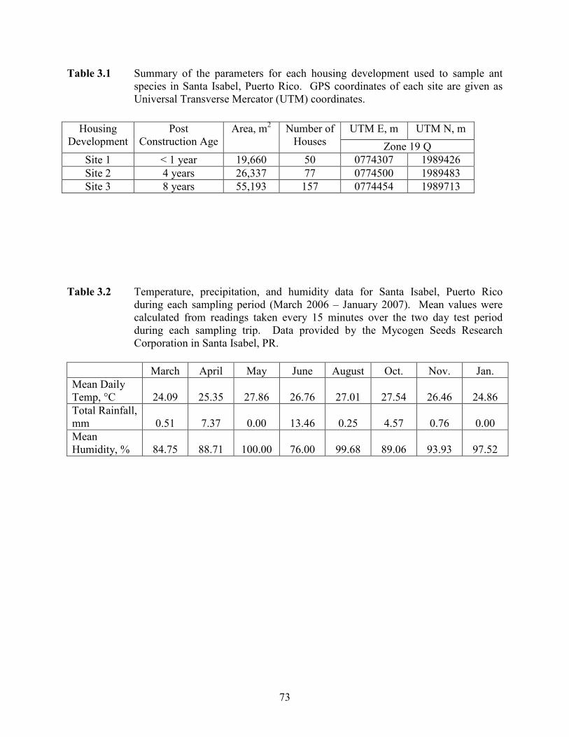
73

Table 3.1 Summary of the parameters for each housing development used to sample ant species in Santa Isabel, Puerto Rico. GPS coordinates of each site are given as Universal Transverse Mercator (UTM) coordinates.

Table 3.2 Temperature, precipitation, and humidity data for Santa Isabel, Puerto Rico during each sampling period (March 2006 – January 2007). Mean values were calculated from readings taken every 15 minutes over the two day test period during each sampling trip. Data provided by the Mycogen Seeds Research Corporation in Santa Isabel, PR.

March April May June August Oct. Nov. Jan.

Mean Daily Temp, °C 24.09 25.35 27.86 26.76 27.01 27.54 26.46 24.86

Total Rainfall, mm 0.51 7.37 0.00 13.46 0.25 4.57 0.76 0.00

Mean Humidity, % 84.75 88.71 100.00 76.00 99.68 89.06 93.93 97.52

UTM E, m UTM N, m Housing Development

Post Construction Age

Area, m2 Number of Houses Zone 19 Q

Site 1 < 1 year 19,660 50 0774307 1989426

Site 2 4 years 26,337 77 0774500 1989483

Site 3 8 years 55,193 157 0774454 1989713

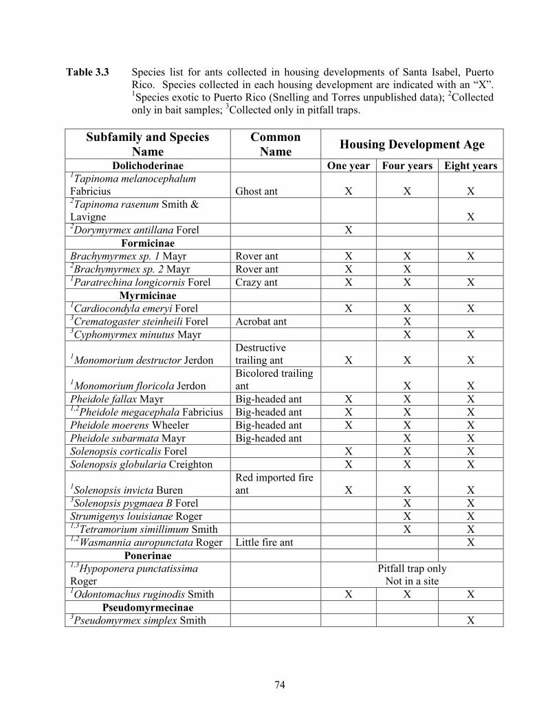
74

Table 3.3 Species list for ants collected in housing developments of Santa Isabel, Puerto Rico. Species collected in each housing development are indicated with an “X”. 1Species exotic to Puerto Rico (Snelling and Torres unpublished data); 2Collected only in bait samples; 3Collected only in pitfall traps.

Subfamily and Species

Name

Common

Name Housing Development Age

Dolichoderinae One year Four years Eight years 1Tapinoma melanocephalum

Fabricius Ghost ant X X X 2Tapinoma rasenum Smith & Lavigne X 2Dorymyrmex antillana Forel X

Formicinae

Brachymyrmex sp. 1 Mayr Rover ant X X X 2Brachymyrmex sp. 2 Mayr Rover ant X X 1Paratrechina longicornis Forel Crazy ant X X X

Myrmicinae 1Cardiocondyla emeryi Forel X X X 3Crematogaster steinheili Forel Acrobat ant X 3Cyphomyrmex minutus Mayr X X

1Monomorium destructor Jerdon

Destructive trailing ant X X X

1Monomorium floricola Jerdon

Bicolored trailing ant X X

Pheidole fallax Mayr Big-headed ant X X X 1,2Pheidole megacephala Fabricius Big-headed ant X X X

Pheidole moerens Wheeler Big-headed ant X X X

Pheidole subarmata Mayr Big-headed ant X X

Solenopsis corticalis Forel X X X

Solenopsis globularia Creighton X X X

1Solenopsis invicta Buren

Red imported fire ant X X X

3Solenopsis pygmaea B Forel X X

Strumigenys louisianae Roger X X 1,3Tetramorium simillimum Smith X X

1,2Wasmannia auropunctata Roger Little fire ant X

Ponerinae 1,3Hypoponera punctatissima

Roger Pitfall trap only Not in a site

1Odontomachus ruginodis Smith X X X

Pseudomyrmecinae 3Pseudomyrmex simplex Smith X

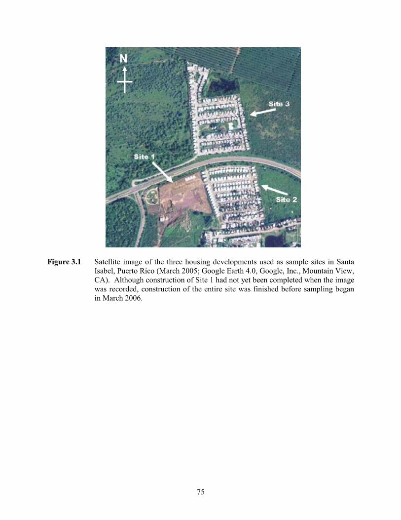
75

NN

Figure 3.1 Satellite image of the three housing developments used as sample sites in Santa Isabel, Puerto Rico (March 2005; Google Earth 4.0, Google, Inc., Mountain View, CA). Although construction of Site 1 had not yet been completed when the image was recorded, construction of the entire site was finished before sampling began in March 2006.

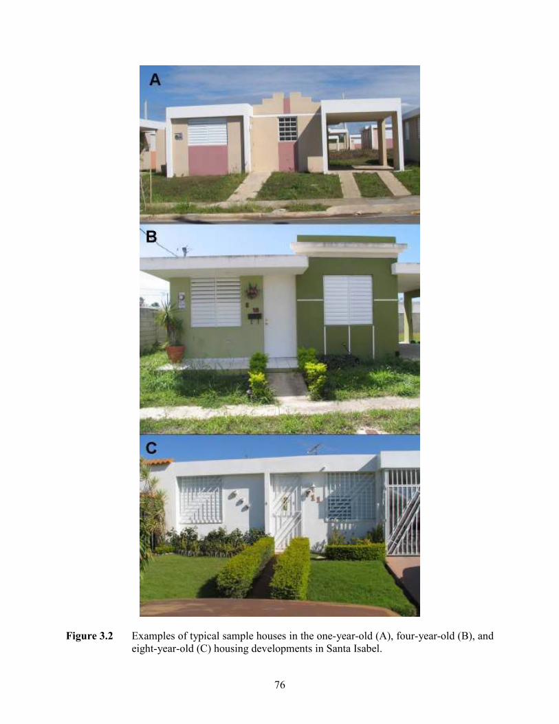
76

Figure 3.2 Examples of typical sample houses in the one-year-old (A), four-year-old (B), and

eight-year-old (C) housing developments in Santa Isabel.

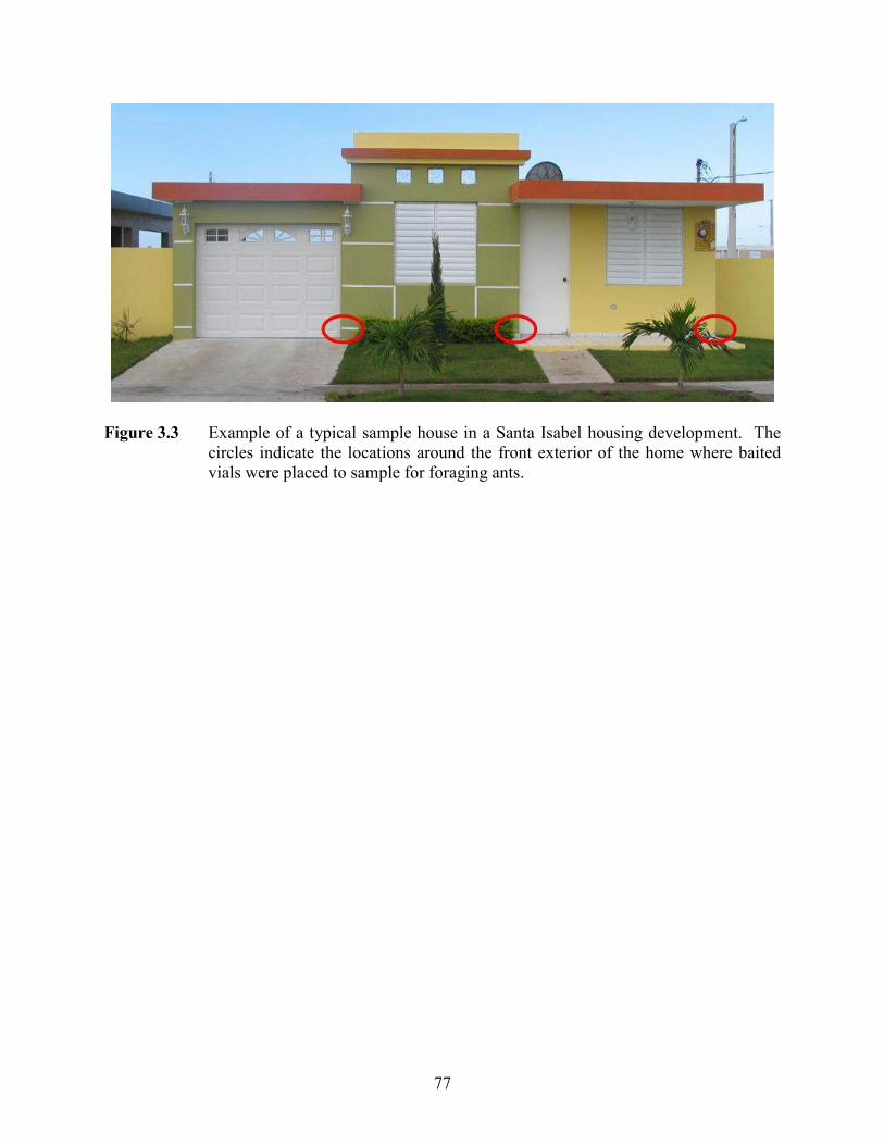
77

Figure 3.3 Example of a typical sample house in a Santa Isabel housing development. The circles indicate the locations around the front exterior of the home where baited vials were placed to sample for foraging ants.

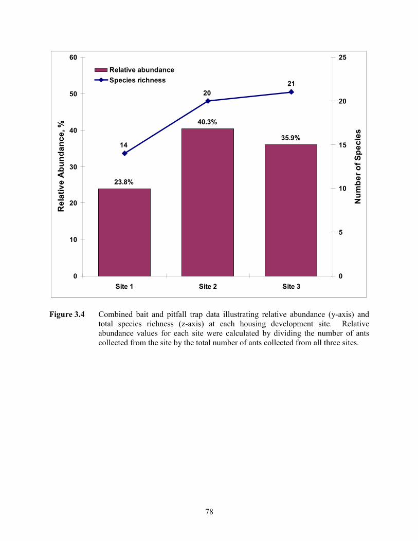
78

35.9%

40.3%

23.8%

21

20

14

0

10

20

30

40

50

60

Site 1 Site 2 Site 3

Relative Abundance, %

0

5

10

15

20

25

Number of Species

Relative abundance

Species richness

Figure 3.4 Combined bait and pitfall trap data illustrating relative abundance (y-axis) and

total species richness (z-axis) at each housing development site. Relative abundance values for each site were calculated by dividing the number of ants collected from the site by the total number of ants collected from all three sites.

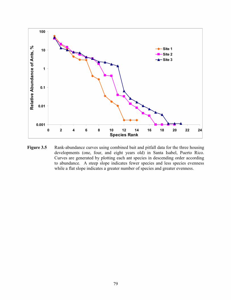
79

0.001

0.01

0.1

1

10

100

0 2 4 6 8 10 12 14 16 18 20 22 24

Species Rank

Relative Abundance of Ants, % Site 1

Site 2

Site 3

Figure 3.5 Rank-abundance curves using combined bait and pitfall data for the three housing developments (one, four, and eight years old) in Santa Isabel, Puerto Rico. Curves are generated by plotting each ant species in descending order according to abundance. A steep slope indicates fewer species and less species evenness while a flat slope indicates a greater number of species and greater evenness.

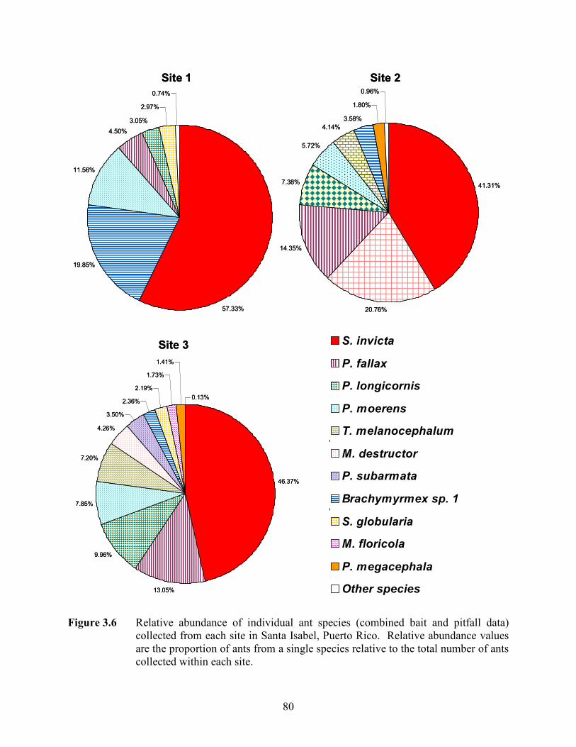
80

Site 3

46.37%

13.05%

9.96%

7.85%

7.20%

4.26%

3.50%

2.36%

2.19%

1.73%

1.41%

0.13%

41.31%

20.76%

14.35%

7.38%

5.72%

4.14%

3.58%

1.80%

0.96%

46.37%

S. invicta

P. fallax

P. longicornis

P. moerens

T. melanocephalum

M. destructor

P. subarmata

Brachymyrmex sp. 1

S. globularia

M. floricola

P. megacephala

Other species

19.85%

11.56%

4.50%

3.05%

2.97%

0.74%

57.33%

Site 1 Site 2

Site 3Site 3

46.37%

13.05%

9.96%

7.85%

7.20%

4.26%

3.50%

2.36%

2.19%

1.73%

1.41%

0.13%

41.31%

20.76%

14.35%

7.38%

5.72%

4.14%

3.58%

1.80%

0.96%

46.37%

S. invicta

P. fallax

P. longicornis

P. moerens

T. melanocephalum

M. destructor

P. subarmata

Brachymyrmex sp. 1

S. globularia

M. floricola

P. megacephala

Other species

19.85%

11.56%

4.50%

3.05%

2.97%

0.74%

57.33%

Site 1 Site 2

Site 3

Figure 3.6 Relative abundance of individual ant species (combined bait and pitfall data)

collected from each site in Santa Isabel, Puerto Rico. Relative abundance values are the proportion of ants from a single species relative to the total number of ants collected within each site.

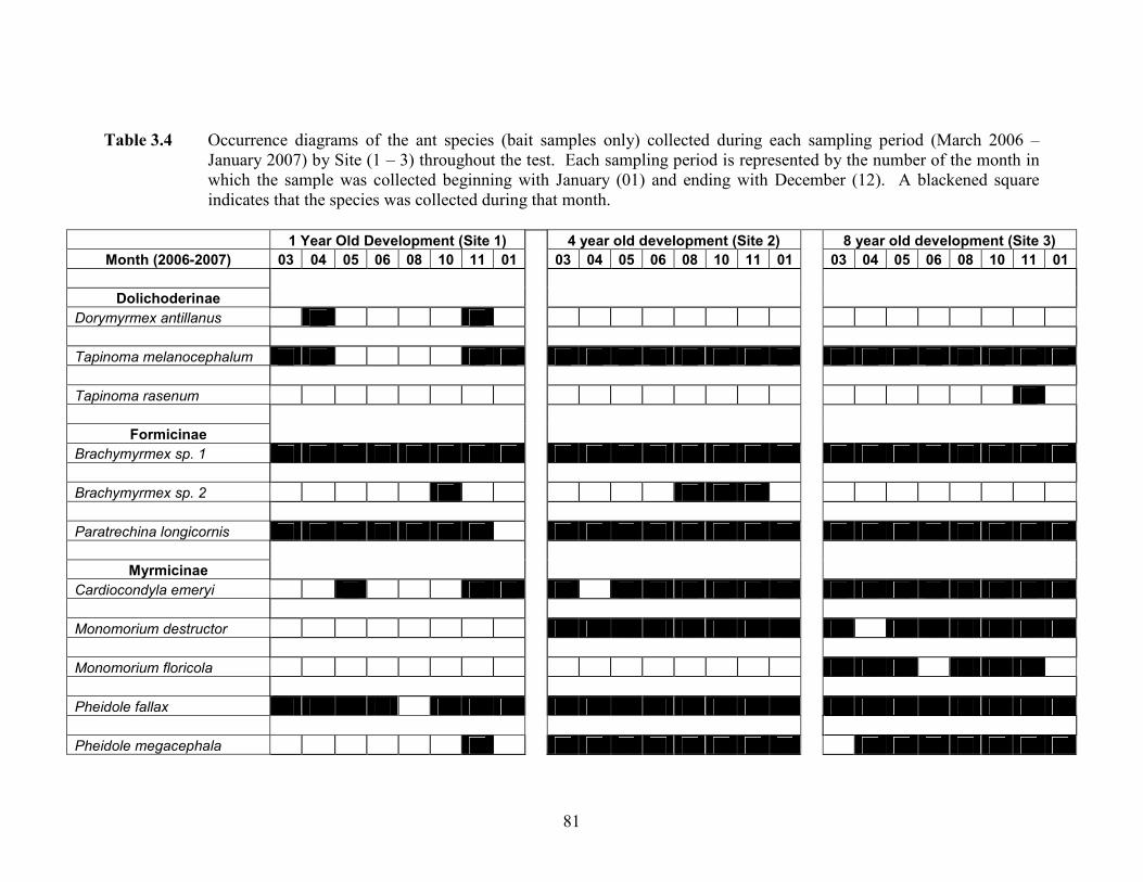
81

Table 3.4 Occurrence diagrams of the ant species (bait samples only) collected during each sampling period (March 2006 – January 2007) by Site (1 – 3) throughout the test. Each sampling period is represented by the number of the month in which the sample was collected beginning with January (01) and ending with December (12). A blackened square indicates that the species was collected during that month.

1 Year Old Development (Site 1) 4 year old development (Site 2) 8 year old development (Site 3)

Month (2006-2007) 03 04 05 06 08 10 11 01 03 04 05 06 08 10 11 01 03 04 05 06 08 10 11 01

Dolichoderinae

Dorymyrmex antillanus

Tapinoma melanocephalum

Tapinoma rasenum

Formicinae

Brachymyrmex sp. 1

Brachymyrmex sp. 2

Paratrechina longicornis

Myrmicinae

Cardiocondyla emeryi

Monomorium destructor

Monomorium floricola

Pheidole fallax

Pheidole megacephala

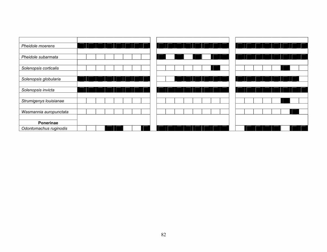
82

Pheidole moerens

Pheidole subarmata

Solenopsis corticalis

Solenopsis globularia

Solenopsis invicta

Strumigenys louisianae

Wasmannia auropunctata

Ponerinae

Odontomachus ruginodis

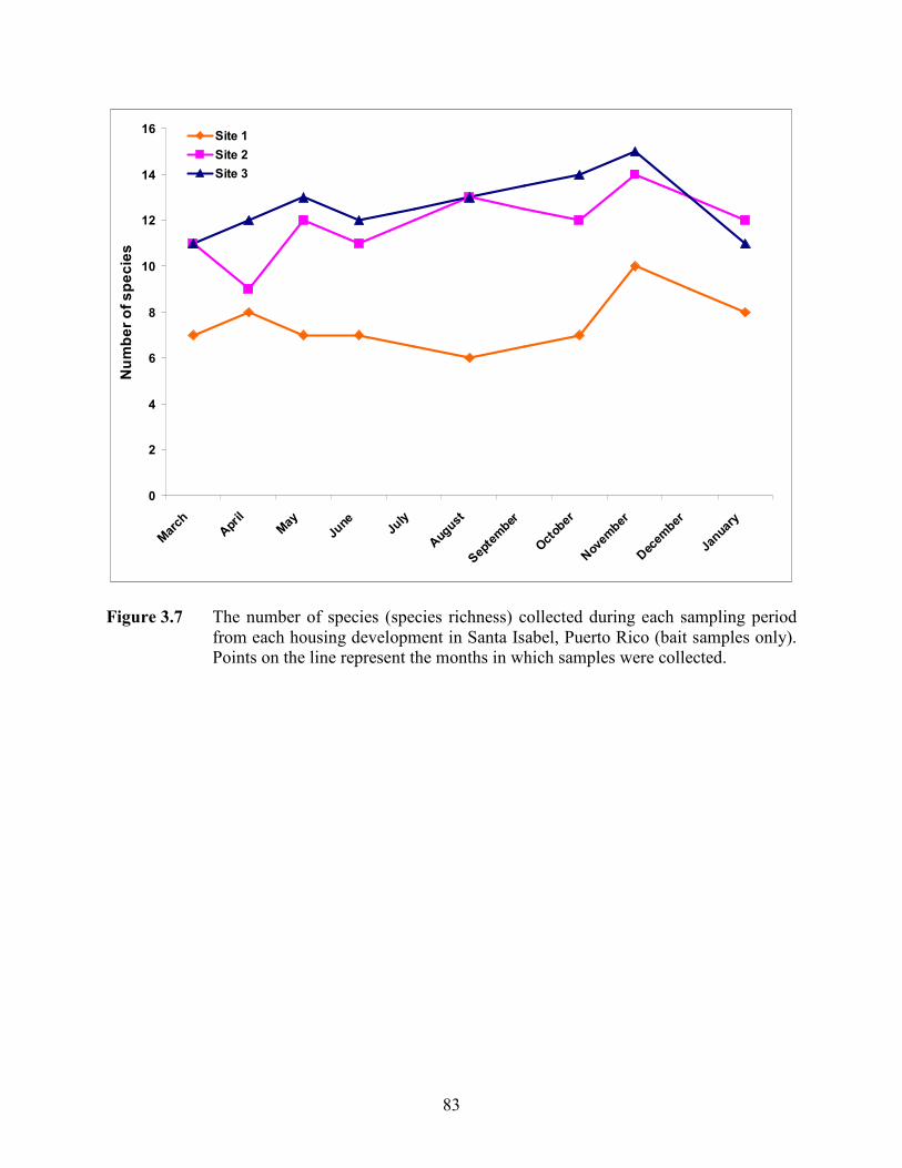
83

0

2

4

6

8

10

12

14

16

March

April

May

June

July

August

September

October

November

December

January

Number of species

Site 1

Site 2

Site 3

Figure 3.7 The number of species (species richness) collected during each sampling period

from each housing development in Santa Isabel, Puerto Rico (bait samples only). Points on the line represent the months in which samples were collected.

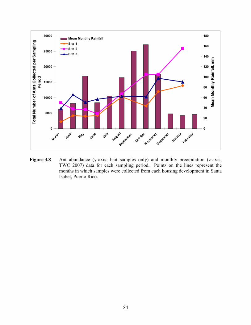
84

0

5000

10000

15000

20000

25000

30000

March

April

May

June

July

August

September

October

November

December

January

February

Total Number of Ants Collected per Sampling

Period

0

20

40

60

80

100

120

140

160

180

Mean Monthly Rainfall, mm

Mean Monthly Rainfall

Site 1

Site 2

Site 3

Figure 3.8 Ant abundance (y-axis; bait samples only) and monthly precipitation (z-axis;

TWC 2007) data for each sampling period. Points on the lines represent the months in which samples were collected from each housing development in Santa Isabel, Puerto Rico.

85

CHAPTER 4. BIODIVERSITY OF ANT SPECIES AT THREE

HOUSING DEVELOPMENTS IN PUERTO RICO:

EFFECT OF HOUSING DEVELOPMENT AGE,

SEASON, BAIT TYPE, AND TIME OF DAY

4.1 Introduction

Ecological succession refers to the orderly and gradual process of change in plant and

animal communities within a biome (Cowles 1911, Golley 1977). Typically, the process of

succession takes place after the formation of a new substrate or a disturbance to an existing

ecosystem (Molles 2005). Currently ecological succession has been divided into two basic

types, primary and secondary succession. Primary succession describes the establishment and

growth of a community on a barren surface usually lacking soil and any pre-existing organisms

(Marrs and Bradshaw 1993, Miles and Walton 1993, Molles 2005). Primary succession may

occur in natural environments such as volcanic ash fields and lava flows or man-made

environments such as rock quarries and china clay sand wastes (Crouch 1993, Del Moral 1993,

Molles 2005, Bradshaw 1993, Marrs and Bradshaw 1993). Secondary succession describes areas

where a disturbance has occurred, destroying a pre-existing community, but the organic matter

was not removed from the soil (Marrs and Bradshaw 1993, Molles 2005). Environments where

secondary succession may occur include land left barren after a forest fire or mudslide, clear-cut

forests, or areas of urban development such as landfills and cemeteries (Marrs and Bradshaw

1993, Molles 2005).

While most studies on ecological succession focus on natural communities (e.g. volcanic

ash fields, abandoned agricultural fields, and clear cut forests), urban succession focuses on

successional processes that take place in urban ecosystems. Urban ecosystems include

residential lawns and gardens, industrial sites, abandoned properties, parks and play grounds,

cemeteries, and waste disposal sites (Nagle 1999). Succession in natural environments may be

caused by natural or man-made disturbances. However, urban succession only occurs after

human disturbance which typically happens during the process of urbanization. During

urbanization, vegetation is removed and the soil is graded. This process leaves a barren substrate

where urban succession can occur. Plants and animals slowly reestablish in the disturbed

ecosystem causing species diversity to increase (Rebele 1994).

86

The stages of succession are highly variable depending on the type of succession

(primary or secondary) and the existing ecosystem (natural or man-made). Bormann and Likens

(1981) described a sequence of stages involved in secondary succession in a disturbed

ecosystem. Bormann and Likens’ (1981) model consists of four stages each based on biomass

accumulation (Figure 2.1): the reorganization, aggradation, transition, and steady-state stages.

The reorganization stage begins when a recently disturbed environment attempts to stabilize.

Once stable, the ecosystem begins to increase in biomass, and continues until biomass

accumulation reaches a peak, and no further biomass (i.e. animal or plant life) can be supported.

This is the aggradation stage. The transition stage is when species interactions begin to change

the species composition of the environment leading to a decline in biomass. Finally, the

community becomes stable and there are no further major increases or decreases in biomass.

This steady-state community is referred to as a climax community and remains as such until

another disturbance takes place (Bormann and Likens 1981, Molles 2005).

Throughout the stages of succession, the species composition or biological diversity of

the environment is changing. Biological diversity, commonly referred to as biodiversity, is a

description of the different species existing in a defined area (i.e. ecosystem, habitat,

environment, community, etc.; Gaston 1996). In general, biodiversity is higher in more complex

environments. Because succession results in an increase of the environmental complexity,

community changes will over time, increase the biodiversity (Molles 2005).

A number of measurements have been developed to assess the biodiversity of a

community. The most common metric used to describe biodiversity is species richness. Species

richness is a count of the number of species in a community or habitat (Molles 2005). Species

evenness is also used to quantify biodiversity and is a comparative value based on the

abundances of each species. Indices of diversity have also been developed to further quantify

biodiversity. These indices, such as the Shannon diversity index, use a combination of richness

and evenness to calculate a diversity value for the community (Molles 2005).

Although biodiversity can be measured based on the entire species composition, some

groups of species, known as indicator species, may also provide an accurate representation of the

diversity within a community (Roth et al. 1994, Lindenmayer et al. 1999). These indicator

species are characterized by being easily collected, and widely distributed throughout the

community. Indicator species also make up a large portion of the total animal biomass, are

87

readily and accurately identified, and respond to environmental change in much the same way as

other organisms within the community (Graham et al. 2004). One group of species that has been

well studied as indicator species for many habitats is the ants (Majer 1981, 1983, 1984, Majer et

al. 1982, Rossbach and Majer 1983, Majer and Brown 1986). A classic study using ants as an

indicator species was conducted by Roth et al. (1994) in Costa Rica. Roth et al. (1994) studied

ant biodiversity in human influenced agricultural and forested field sites to predict the overall

biodiversity of different land management systems. Their study concluded that the ant species

diversity was greater at sites with fewer disturbances and as such, the biodiversity of other

organisms was greater at sites of less disturbance. Therefore, the ant species complex might

successfully be used as an indicator of the overall diversity within a community.

The objective of this study was to quantify the biodiversity of ant species within housing

developments of different ages. We hypothesized that as the age of the housing development

increased, the measures of biodiversity would also increase. Richness, abundance, and diversity

and evenness indices were calculated for each housing development. These indices were then

used to compare the ant species composition between housing developments representing

different stages in the successional process. Monthly changes in species biodiversity were also

compared between sites to determine how the annual change in biodiversity differs as succession

proceeds.

Additional comparisons were made to indirectly assess the biodiversity of the housing

developments of different ages by determining differences in bait preferences and foraging

activity time (morning versus afternoon). We hypothesized that in the early stages of urban

succession, the housing development would be established by generalist ant species. Therefore,

diversity measures would not indicate any significant feeding or foraging preferences. However,

as environmental complexity increases during succession, the habitat will become more diverse

and be able to support specialist ant species with feeding and foraging preferences.


4.2.1 Sampling Protocol


Rico. Sampling methods were conducted as described by Brown (Chapter 1), where sample

homes were selected in Puerto Rican housing developments of different ages (one, four, and

88

eight years old). Baits, consisting of a rope segments soaked in sugar water or peanut oil, were

placed at three locations around the front exterior of each sample house. After one hour, glass

vials containing the baits were collected and filled with isopropyl alcohol (70%), to kill and

preserve any collected ants.

The baiting regimen was conducted twice a day over a two day period at each site. A

total of eight two-day sampling trips were conducted between March 2006 and January 2007. At

the end of each sampling trip, all samples were transported back to the Dodson Urban Pest

Management Laboratory (DUPML) at Virginia Tech. The ant species on each bait were

identified, and the number of individuals in each species was recorded.

4.2.2 Data Analysis

Four measures were selected to quantify the biodiversity of ant species in each of the

housing developments: species richness, S, abundance, N, the Shannon diversity index, H, and

the Shannon evenness index, E. Species richness equaled the total number of ant species

collected from a single house, and abundance equaled the total number of ants collected from the

house. The Shannon diversity index was calculated for each house using the following formula:

∑=

−=S

i

ii ppH1

ln

where pi is the proportion of the individuals of the ith species, and S is the total number of species

(Roth et al. 1994). The Shannon evenness index was calculated for each house using:

SHHHE ln// max ==

where H is the Shannon diversity index, and ln S is the natural logarithm of the number of

species (Roth et al. 1994).

Each house within each of the three sites was sampled at three locations around the

house, using two different types of baits, at two different times during the day, for eight different

months of the year, making this experiment a 3 x 3 x 2 x 2 x 8 factorial experiment. Each

measure of biodiversity (S, N, H, E) was calculated for each house (n = 30) within a site and used

as a single replication. Therefore, 96 (3 x 2 x 2 x 8) samples were taken from each individual

house within a site and pooled together. The pooled data were then used to calculate the

biodiversity measures for each house within each site. The biodiversity measures were then

analyzed statistically using an analysis of variance (ANOVA; SAS Institute 2003) to compare

the measures of biodiversity across each site. Significant differences in the biodiversity

89

measures between sites were compared using Tukey’s method of least squares means (SAS

Institute 2003).

To compare the seasonal changes in biodiversity between the sites, linear regression was

used to plot each biodiversity measure by month and then compare the characteristics of the

regression lines to identify significant differences. For example, richness data were pooled from

12 samples for each house (samples taken from the three locations around the house, using the

two bait types, during two times of the day). The pooled data for each house were then used to

calculate the ant species richness for that house. The richness value of each house (n = 30) was

then averaged to calculate a mean richness value for each combination of site and month (24

values). The eight mean richness values (one for each sampling month) for each site were then

analyzed using linear regression (PROC REG; SAS Institute 2003) to determine the intercept and

slope (regression coefficient) of each regression line. PROC GLM (SAS Institute 2003) was

used to compare the slopes of each regression line and significant differences between sites were

contrasted. This procedure was then repeated for the other three biodiversity measures

(abundance, diversity, and evenness).

To determine the diversity of ants feeding on each bait, the four biodiversity measures

were calculated for each bait type (sugar and peanut oil), nested within each site using a two

factor repeated measures ANOVA (bait, sites). For the analysis on bait type, data from 48

samples (3 x 2 x 8) were combined together for each house (from the three locations around the

house, during the two times of the day, for each of the eight months). The pooled data for each

house were then used to calculate the biodiversity measures for that individual house. The

biodiversity measures of each house (n = 30) were then statistically analyzed to determine

differences in the measures of biodiversity from each bait type. Significant differences in the

biodiversity measures between baits, nested within sites, were compared using Tukey’s method

of least squares means (SAS Institute 2003).

The same procedure was used to determine the ant diversity collected from morning and

afternoon samples. The four biodiversity measures were calculated for time of day (morning and

afternoon) nested within each site using a two factor repeated measures ANOVA (time of day,

sites). For the analysis regarding time of day, data from 48 samples (3 x 2 x 8) were combined

together for each house (from the three locations around the house, from the two bait types, for

each of the eight months). The pooled data for each house were then used to calculate the

90

biodiversity measures for that individual house. The biodiversity measures of each house (n =

30) were then statistically analyzed to determine differences in the measures of biodiversity

between the morning and afternoon sampling times. Significant differences in the biodiversity

measures between time of day, nested within sites, were compared using Tukey’s method of least

squares means (SAS Institute 2003).

4.3 Results

4.3.1 Biodiversity Measures of Each Site

Ant sampling throughout the year resulted in the collection and identification of 243,252

ants from a total of 8,640 bait samples. A total of 19 species were identified from all three sites.

Repeated measures ANOVA determined that the species richness (S) and abundance (N) between

the sites was significantly different (richness: F = 64.27; df = 2, 58; P < 0.0001; abundance: F =

9.48; df = 2, 58; P = 0.0003). The Tukey-Kramer test of least significant difference (LSD)

indicated that significantly fewer species were collected per house at Site 1 compared with Site 2

(P < 0.0001) and Site 3 (P < 0.0001). However, the number of species collected at Site 2 and 3

did not differ significantly from each other (P = 0.0957; Figure 4.1). Similarly, the Tukey-

Kramer LSD test also indicated that the mean abundance of ants collected per house at Site 1

was significantly less than at Site 2 (P = 0.0003) and Site 3 (P = 0.0076). However, the number

of ants collected at Site 2 and 3 did not differ significantly from each other (P = 0.5508; Figure

4.2).

Species diversity (H) and evenness (E) were significantly different between the test sites

(diversity: F = 27.33; df = 2, 58; P < 0.0001; evenness: F = 13.38; df = 2, 58; P < 0.0001). LSD

comparisons of diversity revealed that each site was significantly different from the other two

(Figure 4.3). Site 1 was significantly less diverse than Site 2 (P = 0.0003) and Site 3 (P <

0.0001), and Site 2 was less diverse than Site 3 (P = 0.0062). LSD comparisons conducted on

evenness indices indicated Sites 1 and 2 were not significantly different from each other (P =

0.1496). However, the evenness index for Site 3 was significantly greater than those of Site 1

and 2 (Site 1 and 3: P < 0.0001; Site 2 and 3: P = 0.0056).

4.3.2 Monthly Biodiversity Measures

Mean monthly biodiversity measures were calculated for each site in order to plot

regression lines representing changes in biodiversity over the course of the test period. The

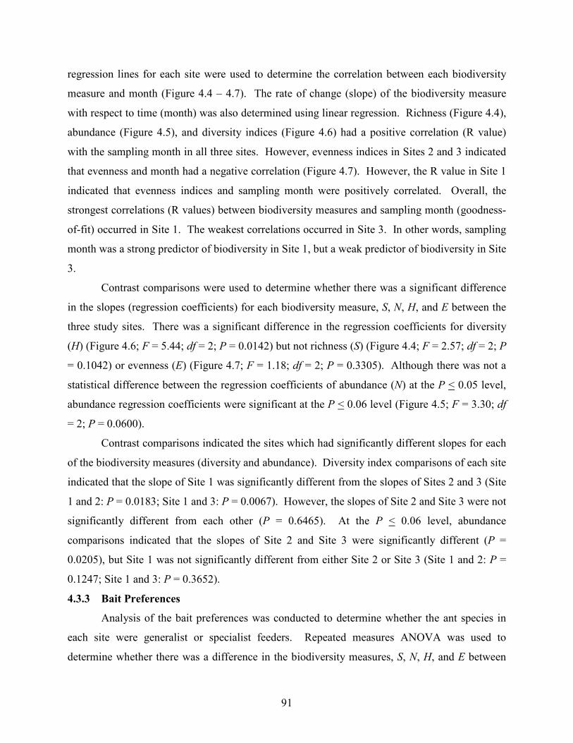
91

regression lines for each site were used to determine the correlation between each biodiversity

measure and month (Figure 4.4 – 4.7). The rate of change (slope) of the biodiversity measure

with respect to time (month) was also determined using linear regression. Richness (Figure 4.4),

abundance (Figure 4.5), and diversity indices (Figure 4.6) had a positive correlation (R value)

with the sampling month in all three sites. However, evenness indices in Sites 2 and 3 indicated

that evenness and month had a negative correlation (Figure 4.7). However, the R value in Site 1

indicated that evenness indices and sampling month were positively correlated. Overall, the

strongest correlations (R values) between biodiversity measures and sampling month (goodness-

of-fit) occurred in Site 1. The weakest correlations occurred in Site 3. In other words, sampling

month was a strong predictor of biodiversity in Site 1, but a weak predictor of biodiversity in Site

3.

Contrast comparisons were used to determine whether there was a significant difference

in the slopes (regression coefficients) for each biodiversity measure, S, N, H, and E between the

three study sites. There was a significant difference in the regression coefficients for diversity

(H) (Figure 4.6; F = 5.44; df = 2; P = 0.0142) but not richness (S) (Figure 4.4; F = 2.57; df = 2; P

= 0.1042) or evenness (E) (Figure 4.7; F = 1.18; df = 2; P = 0.3305). Although there was not a

statistical difference between the regression coefficients of abundance (N) at the P < 0.05 level,

abundance regression coefficients were significant at the P < 0.06 level (Figure 4.5; F = 3.30; df

= 2; P = 0.0600).

Contrast comparisons indicated the sites which had significantly different slopes for each

of the biodiversity measures (diversity and abundance). Diversity index comparisons of each site

indicated that the slope of Site 1 was significantly different from the slopes of Sites 2 and 3 (Site

1 and 2: P = 0.0183; Site 1 and 3: P = 0.0067). However, the slopes of Site 2 and Site 3 were not

significantly different from each other (P = 0.6465). At the P < 0.06 level, abundance

comparisons indicated that the slopes of Site 2 and Site 3 were significantly different (P =

0.0205), but Site 1 was not significantly different from either Site 2 or Site 3 (Site 1 and 2: P =

0.1247; Site 1 and 3: P = 0.3652).

4.3.3 Bait Preferences

Analysis of the bait preferences was conducted to determine whether the ant species in

each site were generalist or specialist feeders. Repeated measures ANOVA was used to

determine whether there was a difference in the biodiversity measures, S, N, H, and E between

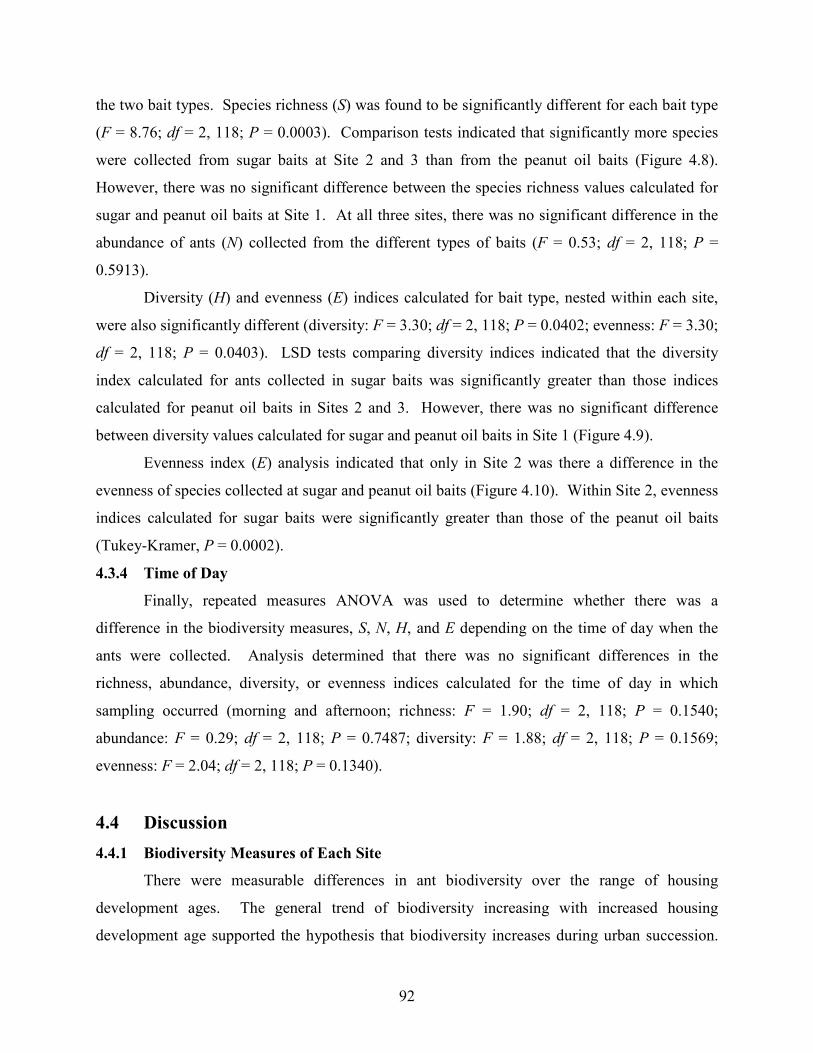
92

the two bait types. Species richness (S) was found to be significantly different for each bait type

(F = 8.76; df = 2, 118; P = 0.0003). Comparison tests indicated that significantly more species

were collected from sugar baits at Site 2 and 3 than from the peanut oil baits (Figure 4.8).

However, there was no significant difference between the species richness values calculated for

sugar and peanut oil baits at Site 1. At all three sites, there was no significant difference in the

abundance of ants (N) collected from the different types of baits (F = 0.53; df = 2, 118; P =

0.5913).

Diversity (H) and evenness (E) indices calculated for bait type, nested within each site,

were also significantly different (diversity: F = 3.30; df = 2, 118; P = 0.0402; evenness: F = 3.30;

df = 2, 118; P = 0.0403). LSD tests comparing diversity indices indicated that the diversity

index calculated for ants collected in sugar baits was significantly greater than those indices

calculated for peanut oil baits in Sites 2 and 3. However, there was no significant difference

between diversity values calculated for sugar and peanut oil baits in Site 1 (Figure 4.9).

Evenness index (E) analysis indicated that only in Site 2 was there a difference in the

evenness of species collected at sugar and peanut oil baits (Figure 4.10). Within Site 2, evenness

indices calculated for sugar baits were significantly greater than those of the peanut oil baits

(Tukey-Kramer, P = 0.0002).

4.3.4 Time of Day

Finally, repeated measures ANOVA was used to determine whether there was a

difference in the biodiversity measures, S, N, H, and E depending on the time of day when the

ants were collected. Analysis determined that there was no significant differences in the

richness, abundance, diversity, or evenness indices calculated for the time of day in which

sampling occurred (morning and afternoon; richness: F = 1.90; df = 2, 118; P = 0.1540;

abundance: F = 0.29; df = 2, 118; P = 0.7487; diversity: F = 1.88; df = 2, 118; P = 0.1569;

evenness: F = 2.04; df = 2, 118; P = 0.1340).

4.4 Discussion

4.4.1 Biodiversity Measures of Each Site

There were measurable differences in ant biodiversity over the range of housing

development ages. The general trend of biodiversity increasing with increased housing

development age supported the hypothesis that biodiversity increases during urban succession.

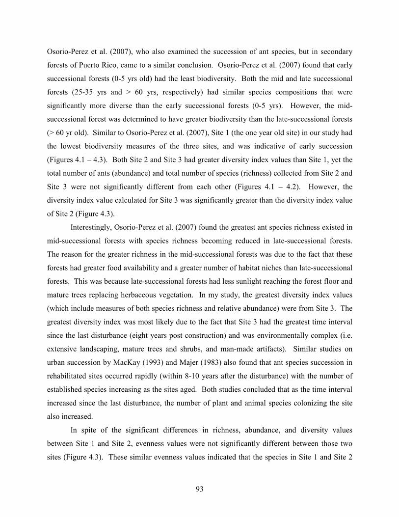
93

Osorio-Perez et al. (2007), who also examined the succession of ant species, but in secondary

forests of Puerto Rico, came to a similar conclusion. Osorio-Perez et al. (2007) found that early

successional forests (0-5 yrs old) had the least biodiversity. Both the mid and late successional

forests (25-35 yrs and > 60 yrs, respectively) had similar species compositions that were

significantly more diverse than the early successional forests (0-5 yrs). However, the mid-

successional forest was determined to have greater biodiversity than the late-successional forests

(> 60 yr old). Similar to Osorio-Perez et al. (2007), Site 1 (the one year old site) in our study had

the lowest biodiversity measures of the three sites, and was indicative of early succession

(Figures 4.1 – 4.3). Both Site 2 and Site 3 had greater diversity index values than Site 1, yet the

total number of ants (abundance) and total number of species (richness) collected from Site 2 and

Site 3 were not significantly different from each other (Figures 4.1 – 4.2). However, the

diversity index value calculated for Site 3 was significantly greater than the diversity index value

of Site 2 (Figure 4.3).

Interestingly, Osorio-Perez et al. (2007) found the greatest ant species richness existed in

mid-successional forests with species richness becoming reduced in late-successional forests.

The reason for the greater richness in the mid-successional forests was due to the fact that these

forests had greater food availability and a greater number of habitat niches than late-successional

forests. This was because late-successional forests had less sunlight reaching the forest floor and

mature trees replacing herbaceous vegetation. In my study, the greatest diversity index values

(which include measures of both species richness and relative abundance) were from Site 3. The

greatest diversity index was most likely due to the fact that Site 3 had the greatest time interval

since the last disturbance (eight years post construction) and was environmentally complex (i.e.

extensive landscaping, mature trees and shrubs, and man-made artifacts). Similar studies on

urban succession by MacKay (1993) and Majer (1983) also found that ant species succession in

rehabilitated sites occurred rapidly (within 8-10 years after the disturbance) with the number of

established species increasing as the sites aged. Both studies concluded that as the time interval

increased since the last disturbance, the number of plant and animal species colonizing the site

also increased.

In spite of the significant differences in richness, abundance, and diversity values

between Site 1 and Site 2, evenness values were not significantly different between those two

sites (Figure 4.3). These similar evenness values indicated that the species in Site 1 and Site 2

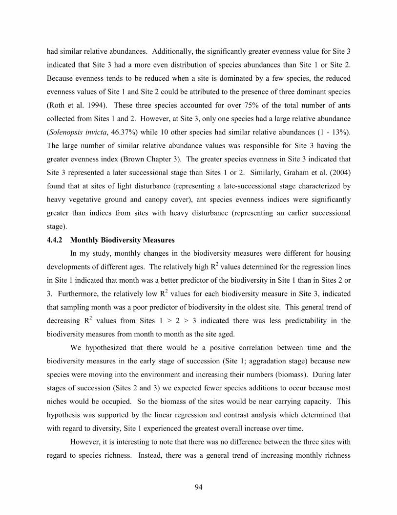
94

had similar relative abundances. Additionally, the significantly greater evenness value for Site 3

indicated that Site 3 had a more even distribution of species abundances than Site 1 or Site 2.

Because evenness tends to be reduced when a site is dominated by a few species, the reduced

evenness values of Site 1 and Site 2 could be attributed to the presence of three dominant species

(Roth et al. 1994). These three species accounted for over 75% of the total number of ants

collected from Sites 1 and 2. However, at Site 3, only one species had a large relative abundance

(Solenopsis invicta, 46.37%) while 10 other species had similar relative abundances (1 - 13%).

The large number of similar relative abundance values was responsible for Site 3 having the

greater evenness index (Brown Chapter 3). The greater species evenness in Site 3 indicated that

Site 3 represented a later successional stage than Sites 1 or 2. Similarly, Graham et al. (2004)

found that at sites of light disturbance (representing a late-successional stage characterized by

heavy vegetative ground and canopy cover), ant species evenness indices were significantly

greater than indices from sites with heavy disturbance (representing an earlier successional

stage).

4.4.2 Monthly Biodiversity Measures

In my study, monthly changes in the biodiversity measures were different for housing

developments of different ages. The relatively high R2 values determined for the regression lines

in Site 1 indicated that month was a better predictor of the biodiversity in Site 1 than in Sites 2 or

3. Furthermore, the relatively low R2 values for each biodiversity measure in Site 3, indicated

that sampling month was a poor predictor of biodiversity in the oldest site. This general trend of

decreasing R2 values from Sites 1 > 2 > 3 indicated there was less predictability in the

biodiversity measures from month to month as the site aged.

We hypothesized that there would be a positive correlation between time and the

biodiversity measures in the early stage of succession (Site 1; aggradation stage) because new

species were moving into the environment and increasing their numbers (biomass). During later

stages of succession (Sites 2 and 3) we expected fewer species additions to occur because most

niches would be occupied. So the biomass of the sites would be near carrying capacity. This

hypothesis was supported by the linear regression and contrast analysis which determined that

with regard to diversity, Site 1 experienced the greatest overall increase over time.

However, it is interesting to note that there was no difference between the three sites with

regard to species richness. Instead, there was a general trend of increasing monthly richness

95

values throughout the test period in each site. This increase in richness may be attributed to the

fact that the number of species collected from each house in the three sites increased as the site

aged over the year. This increase in richness can occur if either more species move into the site,

or if the species already present at the site spread out to more houses. In either case, an increase

in the mean number of species present at an individual sample house would cause the richness of

that sample house to increase. Brown (Chapter 3) found that new species additions were not

common in any site during the test. Therefore, it was concluded that the overall increased

richness observed over the test period was the result of species which were already in the site,

expanding their foraging range to new houses.

There was also a general trend of increasing abundance values in each site over the test

period indicating an annual cycle of colony growth in each site. Because the mean number of

ants collected at each sample house in a site was relatively low in March when compared to later

months of the year, we concluded that these increases in abundance were attributed to a seasonal

colony growth cycle (Brown Chapter 3). Interestingly, the slope of the regression line for Site 2

was significantly greater than the slope of the regression line for Site 3 at the P > 0.06 level. The

greater slope of Site 2 indicated that the rate in which ant abundance increased over the year was

greater in Site 2 than in Site 3. This difference in the rate of increasing ant abundance suggested

that these sites represented different stages of succession. The large increases in ant abundance

in Site 2 indicated that resources were still available for to support additional biomass.

Therefore, Site 2 represents a period near the peak of the aggradation stage or beginning of the

transition stage (Bormann and Likens 1981). The general increases in ant abundance in Site 3

appeared to be much more stable over the year. Site 3 likely had fewer resources available to

support additional biomass because most resources were already at carrying capacity. The

possibility that Site 3 was already at carrying capacity may have prevented the production of a

large number of additional ant workers in Site 3. Thus, Site 3 most likely represents a later phase

of the transition stage in the successional process. The hypothesis that Site 3 represented a

habitat in the transition stage was also supported by the rank-abundance curves and diversity

indices presented in Chapters 3 and 4.

The regression analysis for diversity indices also indicated that diversity increased with

each sampling period in all sites. Similar to the richness analysis, the positive diversity slopes

were due to the species expanding throughout the site and increasing their numbers at each house

96

within the sites. Although all three sites had positive slopes (indicating increasing diversity), the

slope of Site 1 was significantly greater than Site 2 and 3. The greater regression coefficient for

Site 1 implies that the ant species were expanding their range and numbers more rapidly

throughout Site 1. This increase in foraging range is indicative of the aggradation stage of

succession (Bormann and Likens 1981). Because Site 1 was recovering from a recent

disturbance (construction of the development), we would expect newly established species to

increase their range within the site over time.

Sites 2 and 3 had more consistent measures of diversity over the test period, indicating

little change in the number and abundance of species collected from one sampling period to the

next. The relatively flat slope of the regression line indicated that no new species were moving

into the older sites, and those species which were already present were no longer expanding their

range. The reason for this stasis in biodiversity was most likely due to the fact that there were

few available resources in these fully inhabited sites. Similar to my study, Majer (1983)

documented the rapid establishment of 29 new ant species in rehabilitated mines in Northern

Australia within 1.5 years. However, at mining sites that had been rehabilitated for longer

periods (between 3.5 and 7.5 yrs), the addition of new species were much less frequent (in one

site only three new species were collected over a two year period). Both the current study and

that of Majer (1983) provide evidence that the ant species complex in older sites is more stable

than sites which have been more recently disturbed.

The regression and contrast analysis for species evenness indices indicated no significant

difference between the three sites. Therefore, the rate at which evenness was changing over the

test period was the same across all three sites. Although the rates of change were not

significantly different, the slope for Site 1 was slightly positive while the slopes for Sites 2 and 3

were slightly negative. These differences in slopes suggested that species evenness was

increasing in Site 1 as the year progressed. However in Sites 2 and 3, the negative slopes

suggested that evenness may have been decreasing over the year. The ability of some species

(e.g. S. invicta; Tschinkel 2006) to produce a greater number of workers than other species over

the course of the year could be the cause of this negative correlation between evenness and

month in the older sites. However, it must be considered that the slopes for the three sites were

not significantly different and the R2 values for Sites 2 and 3 were very low indicating that the

line slopes were not necessarily good predictors of the evenness trends.

97

4.4.3 Bait Preferences

As habitats increase in complexity, a greater variety of food recourses become available.

Ant species that prefer these different types of food resources are those most likely to become

established in these habitats. Therefore, the feeding preferences of ant species within a habitat

are likely to represent the diversity of that habitat, both in the habitat’s food resource diversity,

and the environmental diversity as it relates to the stages of succession. Early successional

habitats have less environmental complexity (Molles 2005). Therefore, there are fewer food

sources and microhabitat niches to support a diverse fauna of ants. Thus, the ant species that are

present in early successional habitats tend to be generalist species. However, later successional

habitats, which tend to have greater environmental complexity (Molles), are able to support a

greater diversity of ant species because of the greater diversity of food resources and

microhabitat niches available to resident species. Therefore, these later successional habitats are

able to support ant species with specialized nesting and feeding preferences.

MacKay (1993), when studying ant species succession on nuclear waste sites, identified

five “weedy” species which are characteristic of early succession. MacKay (1993) determined

that these five species were scavengers and represented generalist feeders. Similar to MacKay

(1993), Majer (1983) also identified many generalist, ground-foraging ant species in the early

stages of bauxite mine rehabilitation. In contrast to these generalist species found in early-

succession habitats, ants with specialized feeding preferences tend to colonize habitats that are in

the later stages of succession. In nuclear waste sites that had been abandoned for 10 years,

MacKay (1993), found two ant species that were specialized parasites of other ants. The

presence of these parasitic species was indicative of an environment that was not only complex

enough to support the parasitic species but also their host species. This specialized parasite-host

relationship could only evolve within a habitat in the later stages of secondary succession.

Studies by Majer (1983) and Majer and Brown (1986) also identified specialist ant species in

rehabilitated mine sites and gardens. These habitats had a high diversity of plant fauna and

vegetative complexity (the addition of shrubs and leaf litter). Specialist ant species were

identified nesting in the leaves and branches of shrubs. Other colonies of cryptic species were

found nesting in the accumulated leaf litter. These same species were not collected in early

successional habitats because their specialized nesting sites were not yet available. A similar

study by Osorio-Perez et al. (2007) in secondary forests identified three specialist ant species,

98

those that nest in trees, those that nest only in rotten logs and stumps, and those that feed only on

fungus cultured on caterpillar feces. Osorio-Perez et al. (2007) concluded that greater ant species

richness in secondary forests >25 years was due to the availability of specialized food sources.

In each of these studies, the researchers concluded that later stages of succession had greater ant

diversity due to the greater habitat complexity. The greater complexity resulted in a variety of

feeding and nesting resources which facilitated the establishment of ant species with specialized

preferences.

In my study, species bait preferences within the three different sites were indicative of the

resources available in those sites. At Site 1, there was no difference in the richness values

calculated for ants feeding on sugar or peanut oil baits. Therefore, we could not identify a

feeding preference among ant species at Site 1 and concluded that those species were most likely

generalist species. Because Site 1 represented an early stage of succession characterized by the

recent invasion of founding species, we expected the ant fauna to consist mostly of generalists

(Majer 1983). It should be noted that the plant fauna of Site 1 was extremely limited with only

grasses and other weedy plant species observed inhabiting the site. No other food resources were

observed. However, in pitfall traps placed throughout Site 1, additional small arthropod species

(beetles, millipedes, spiders) were collected which likely provided additional food sources for the

newly established ant colonies. These limited plant and animal food resources at Site 1, most

likely could only support ant species that were generalist feeders and not those species that

would require a more specialized diet (Smith 1965, Klotz 2004).

At Sites 2 and 3, the species richness and diversity indices calculated for the sugar baits

were significantly greater than those calculated for peanut oil baits. This preference for sugar

food sources indicates a greater number of ant species were sugar feeders. The establishment of

sugar feeding ants at these sites may have been due to the presence of carbohydrate food sources

such as flowering plants which provide nectar, and ornamental plants with extrafloral nectaries.

The presence of these plants throughout the landscaping may have allowed for specialist sweet

feeders, such as P. longicornis and T. melanocephalum (Klotz 2004), to become established at

these older sites.

Overall, the richness and diversity indices calculated for baits at Site 1 indicated that the

founding species were generalist feeders. However, as succession progressed (at Sites 2 and 3),

the subsequent ant species (e.g. P. longicornis) were more specialized in their preference for

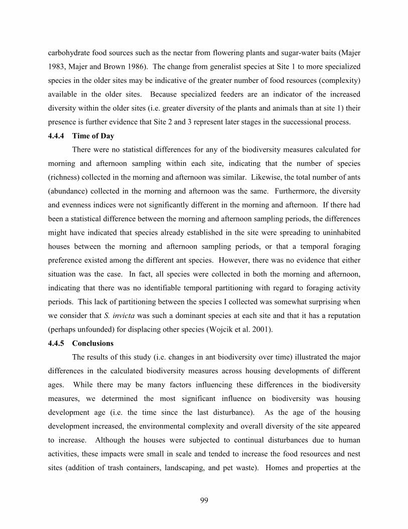
99

carbohydrate food sources such as the nectar from flowering plants and sugar-water baits (Majer

1983, Majer and Brown 1986). The change from generalist species at Site 1 to more specialized

species in the older sites may be indicative of the greater number of food resources (complexity)

available in the older sites. Because specialized feeders are an indicator of the increased

diversity within the older sites (i.e. greater diversity of the plants and animals than at site 1) their

presence is further evidence that Site 2 and 3 represent later stages in the successional process.

4.4.4 Time of Day

There were no statistical differences for any of the biodiversity measures calculated for

morning and afternoon sampling within each site, indicating that the number of species

(richness) collected in the morning and afternoon was similar. Likewise, the total number of ants

(abundance) collected in the morning and afternoon was the same. Furthermore, the diversity

and evenness indices were not significantly different in the morning and afternoon. If there had

been a statistical difference between the morning and afternoon sampling periods, the differences

might have indicated that species already established in the site were spreading to uninhabited

houses between the morning and afternoon sampling periods, or that a temporal foraging

preference existed among the different ant species. However, there was no evidence that either

situation was the case. In fact, all species were collected in both the morning and afternoon,

indicating that there was no identifiable temporal partitioning with regard to foraging activity

periods. This lack of partitioning between the species I collected was somewhat surprising when

we consider that S. invicta was such a dominant species at each site and that it has a reputation

(perhaps unfounded) for displacing other species (Wojcik et al. 2001).

4.4.5 Conclusions

The results of this study (i.e. changes in ant biodiversity over time) illustrated the major

differences in the calculated biodiversity measures across housing developments of different

ages. While there may be many factors influencing these differences in the biodiversity

measures, we determined the most significant influence on biodiversity was housing

development age (i.e. the time since the last disturbance). As the age of the housing

development increased, the environmental complexity and overall diversity of the site appeared

to increase. Although the houses were subjected to continual disturbances due to human

activities, these impacts were small in scale and tended to increase the food resources and nest

sites (addition of trash containers, landscaping, and pet waste). Homes and properties at the

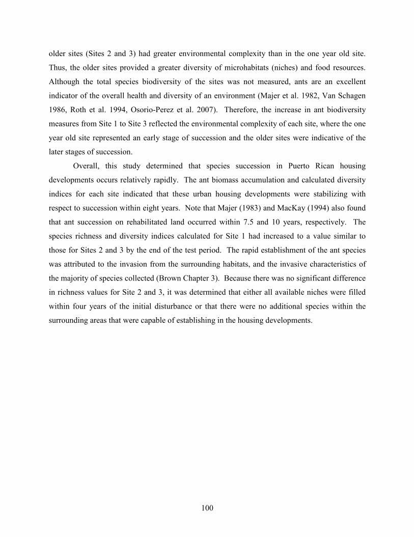
100

older sites (Sites 2 and 3) had greater environmental complexity than in the one year old site.

Thus, the older sites provided a greater diversity of microhabitats (niches) and food resources.

Although the total species biodiversity of the sites was not measured, ants are an excellent

indicator of the overall health and diversity of an environment (Majer et al. 1982, Van Schagen

1986, Roth et al. 1994, Osorio-Perez et al. 2007). Therefore, the increase in ant biodiversity

measures from Site 1 to Site 3 reflected the environmental complexity of each site, where the one

year old site represented an early stage of succession and the older sites were indicative of the

later stages of succession.

Overall, this study determined that species succession in Puerto Rican housing

developments occurs relatively rapidly. The ant biomass accumulation and calculated diversity

indices for each site indicated that these urban housing developments were stabilizing with

respect to succession within eight years. Note that Majer (1983) and MacKay (1994) also found

that ant succession on rehabilitated land occurred within 7.5 and 10 years, respectively. The

species richness and diversity indices calculated for Site 1 had increased to a value similar to

those for Sites 2 and 3 by the end of the test period. The rapid establishment of the ant species

was attributed to the invasion from the surrounding habitats, and the invasive characteristics of

the majority of species collected (Brown Chapter 3). Because there was no significant difference

in richness values for Site 2 and 3, it was determined that either all available niches were filled

within four years of the initial disturbance or that there were no additional species within the

surrounding areas that were capable of establishing in the housing developments.

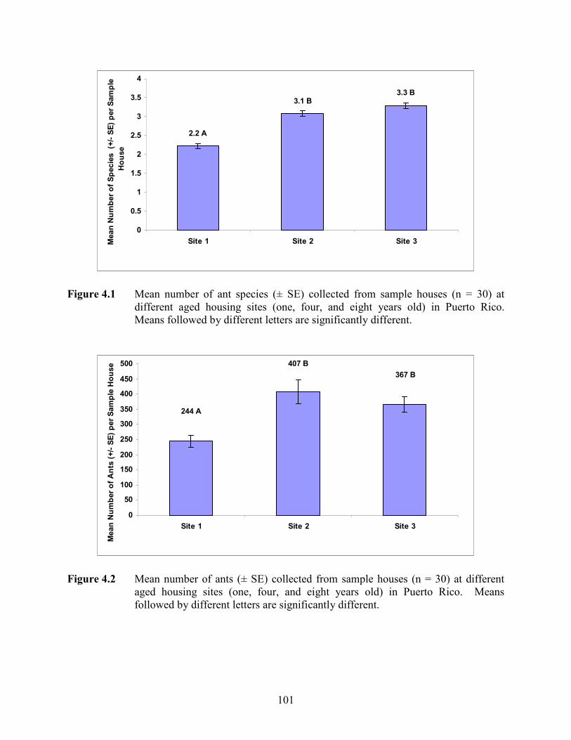
101

3.1 B3.3 B

2.2 A

0

0.5

1

1.5

2

2.5

3

3.5

4

Site 1 Site 2 Site 3Mean Number of Species (+/- SE) per Sample

House

Figure 4.1 Mean number of ant species (± SE) collected from sample houses (n = 30) at different aged housing sites (one, four, and eight years old) in Puerto Rico. Means followed by different letters are significantly different.

367 B

407 B

244 A

0

50

100

150

200

250

300

350

400

450

500


Mean Number of Ants (+/- SE) per Sample House

Figure 4.2 Mean number of ants (± SE) collected from sample houses (n = 30) at different aged housing sites (one, four, and eight years old) in Puerto Rico. Means followed by different letters are significantly different.

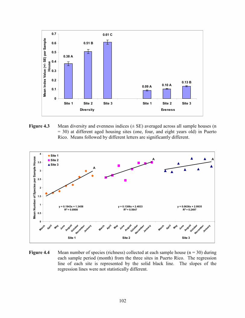
102

0.13 B0.10 A0.09 A

0.61 C

0.51 B

0.38 A

0

0.1

0.2

0.3

0.4

0.5

0.6

0.7

Site 1 Site 2 Site 3 Site 1 Site 2 Site 3

Diversity Eveness

Mean Index Value (+/- SE) per Sample

House

Figure 4.3 Mean diversity and evenness indices (± SE) averaged across all sample houses (n

= 30) at different aged housing sites (one, four, and eight years old) in Puerto Rico. Means followed by different letters are significantly different.

0

0.5

1

1.5

2

2.5

3

3.5

4

March

April

May

June

August

October

November

January

March

April

May

June

August

October

November

January

March

April

May

June

August

October

November

January


Mean Number of Species per Sample House Site 1

Site 2

Site 3

y = 0.0636x + 2.9935

R2 = 0.2497

y = 0.1306x + 2.4833

R2 = 0.5647

y = 0.1943x + 1.3458

R2 = 0.8908

A

A A

0

0.5

1

1.5

2

2.5

3

3.5

4

March

April

May

June

August

October

November

January

March

April

May

June

August

October

November

January

March

April

May

June

August

October

November

January


Mean Number of Species per Sample House Site 1

Site 2

Site 3

y = 0.0636x + 2.9935

R2 = 0.2497

y = 0.1306x + 2.4833

R2 = 0.5647

y = 0.1943x + 1.3458

R2 = 0.8908

A

A A

Figure 4.4 Mean number of species (richness) collected at each sample house (n = 30) during each sample period (month) from the three sites in Puerto Rico. The regression line of each site is represented by the solid black line. The slopes of the regression lines were not statistically different.

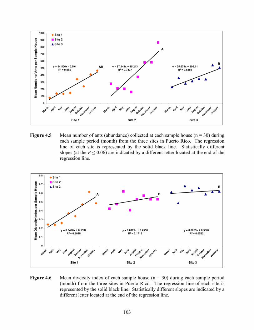
103

0

100

200

300

400

500

600

700

800

900

1000

March

April

May

June

August

October

November

January

March

April

May

June

August

October

November

January

March

April

May

June

August

October

November

January


Mean Number of Ants per Sample House

Site 1

Site 2

Site 3

y = 35.679x + 206.11

R2 = 0.6889

y = 87.143x + 15.243

R2 = 0.7437

y = 54.506x - 0.794

R2 = 0.855AB

A

B

0

100

200

300

400

500

600

700

800

900

1000

March

April

May

June

August

October

November

January

March

April

May

June

August

October

November

January

March

April

May

June

August

October

November

January


Mean Number of Ants per Sample House

Site 1

Site 2

Site 3

y = 35.679x + 206.11

R2 = 0.6889

y = 87.143x + 15.243

R2 = 0.7437

y = 54.506x - 0.794

R2 = 0.855AB

A

B

Figure 4.5 Mean number of ants (abundance) collected at each sample house (n = 30) during

each sample period (month) from the three sites in Puerto Rico. The regression line of each site is represented by the solid black line. Statistically different slopes (at the P < 0.06) are indicated by a different letter located at the end of the regression line.

0

0.1

0.2

0.3

0.4

0.5

0.6

0.7

0.8

March

April

May

June

August

October

November

January

March

April

May

June

August

October

November

January

March

April

May

June

August

October

November

January


Mean Diversity Index per Sample House

Site 1

Site 2

Site 3

y = 0.0055x + 0.5882

R2 = 0.0522

y = 0.0122x + 0.4558

R2 = 0.1715

y = 0.0496x + 0.1537

R2 = 0.8018

A B

B

0

0.1

0.2

0.3

0.4

0.5

0.6

0.7

0.8

March

April

May

June

August

October

November

January

March

April

May

June

August

October

November

January

March

April

May

June

August

October

November

January


Mean Diversity Index per Sample House

Site 1

Site 2

Site 3

y = 0.0055x + 0.5882

R2 = 0.0522

y = 0.0122x + 0.4558

R2 = 0.1715

y = 0.0496x + 0.1537

R2 = 0.8018

A B

B

Figure 4.6 Mean diversity index of each sample house (n = 30) during each sample period

(month) from the three sites in Puerto Rico. The regression line of each site is represented by the solid black line. Statistically different slopes are indicated by a different letter located at the end of the regression line.

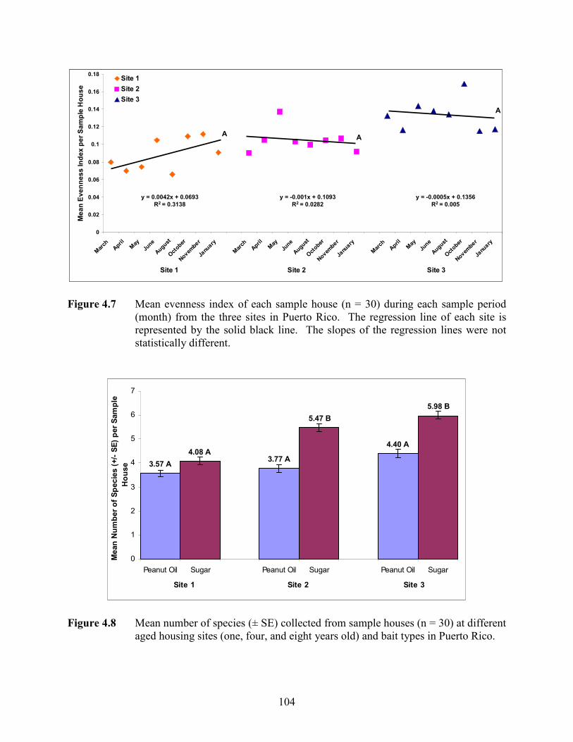
104

0

0.02

0.04

0.06

0.08

0.1

0.12

0.14

0.16

0.18

March

April

May

June

August

October

November

January

March

April

May

June

August

October

November

January

March

April

May

June

August

October

November

January


Mean Evenness Index per Sample House

Site 1

Site 2

Site 3

y = -0.0005x + 0.1356

R2 = 0.005

y = 0.0042x + 0.0693

R2 = 0.3138

y = -0.001x + 0.1093

R2 = 0.0282

AA

A

0

0.02

0.04

0.06

0.08

0.1

0.12

0.14

0.16

0.18

March

April

May

June

August

October

November

January

March

April

May

June

August

October

November

January

March

April

May

June

August

October

November

January


Mean Evenness Index per Sample House

Site 1

Site 2

Site 3

y = -0.0005x + 0.1356

R2 = 0.005

y = 0.0042x + 0.0693

R2 = 0.3138

y = -0.001x + 0.1093

R2 = 0.0282

AA

A

Figure 4.7 Mean evenness index of each sample house (n = 30) during each sample period

(month) from the three sites in Puerto Rico. The regression line of each site is represented by the solid black line. The slopes of the regression lines were not statistically different.

5.98 B

4.40 A

5.47 B

3.77 A4.08 A

3.57 A

0

1

2

3

4

5

6

7

Peanut Oil Sugar Peanut Oil Sugar Peanut Oil Sugar


Mean Number of Species (+/- SE) per Sample

House

Figure 4.8 Mean number of species (± SE) collected from sample houses (n = 30) at different

aged housing sites (one, four, and eight years old) and bait types in Puerto Rico.

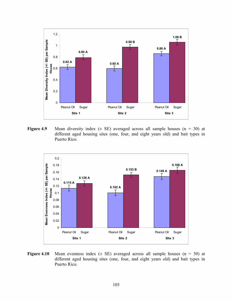
105

1.06 B

0.86 A

0.98 B

0.60 A

0.80 A

0.62 A

0

0.2

0.4

0.6

0.8

1

1.2



Mean Diversity Index (+/- SE) per Sample

House

Figure 4.9 Mean diversity index (± SE) averaged across all sample houses (n = 30) at

different aged housing sites (one, four, and eight years old) and bait types in Puerto Rico.

0.166 A

0.149 A0.153 B

0.102 A

0.128 A

0.115 A

0

0.02

0.04

0.06

0.08

0.1

0.12

0.14

0.16

0.18

0.2



Mean Evenness Index (+/- SE) per Sample

House

Figure 4.10 Mean evenness index (± SE) averaged across all sample houses (n = 30) at

different aged housing sites (one, four, and eight years old) and bait types in Puerto Rico.

106

CHAPTER 5. SPATIAL DISTRIBUTION OF ANT FORAGING

RANGES AS AN INDICATOR OF HOUSING

DEVELOPMENT STAGE OF SUCCESSION

5.1 Introduction

Territoriality is a universal behavior among ant species (Holldobler and Wilson 1990). In

fact, Holldobler and Wilson (1990) explained that territorial behavior has evolved to a greater

degree in ants than most solitary animals. The territories of ant species within a community tend

to be highly structured due to competition (Adams 1994). Most often a territory is defined and

defended by worker ants that patrol around the border (Carroll and Janzen 1973). The purpose

of patrolling is to defend the colony’s territory from potential invaders. In the case of Azteca

trigona, major workers are typically found in greater abundances around the perimeter of the

colony’s territory than among the foraging trails within the interior (Adams 1994).

Competition over foraging territories is generally categorized as intraspecific (same

species) or interspecific (different species) (Holldobler and Wilson 1990, Adams 1994). The

existence of multiple defined territories within an ant community is the result of intra- or

interspecific interactions. These interactions are based on the characteristics (i.e. aggressiveness,

foraging style, colony size, monogyne or polygyne, feeding preferences) of the ant species within

the community (Carroll and Janzen 1973, Briese and Macauley 1977, Levings and Traniello

1981). Thus, depending on the species that are present in a localized area, a defined territory

may cover a huge area (as large as 1,600 square meters) or may only be as large as the immediate

vicinity of a nest (Holldobler and Wilson 1990).

One of the most well documented examples of ant territoriality was found in the spatial

distribution of tropical arboreal species in tree crop plantations (Jackson 1984, Holldobler and

Wilson 1990, Adams 1994). Within these plantations, intra- and interspecific competition

resulted in well defined boundaries of one ant colony per tree. These boundaries formed a

mosaic of ant territories with very little overlap of different species. Known as the “ant mosaic

hypothesis”, this hypothesis predicted that the dominant species in the plantation exclusively

defend their territories with little to no overlap of common territories within the forest canopy

(Adams 1994).

107

Although these absolute territories (territories which are defended all the time; Holldobler

and Wilson 1990) were present in canopy dwelling ant species, studies investigating ground

dwelling species indicated an overlap of territories (Jackson 1984). Although Jackson (1984)

documented that competition also occurred between ground dwelling species, the individual

species’ territories were found to spatially overlap in the majority of cases. Holldobler and

Wilson (1990) indicated that these types of overlapping territories are spatiotemporal.

Spatiotemporal territoriality occurs when different sections of a colony’s territory are defended at

different times. Thus, a partitioning can occur between species allowing one species to forage in

an area during one part of the day, and then another species to forage in the same area at a

different time of day. Spatiotemporal territoriality is commonly observed with nocturnal and

diurnal species of Camponotus that partition their foraging time in order to avoid competition

with other species for the same food resources (Carroll and Janzen 1973).

While territories may be defended absolutely or based on spatiotemporal characteristics

of the species involved, the territorial boundaries also change over time due to the colony’s

development and environmental conditions (Briese and Macauley 1977). As individual workers

explore new locations, their foraging range increases as they become familiar with the new

terrain and their territorial boundaries expand (Carroll and Janzen 1973). Territorial behavior, in

the form of worker aggressiveness, has also been found to change based on the stages of colony

growth (Carroll and Janzen 1973, Holldobler and Wilson 1990). For example, when Formica

reproductives were being produced, Formica workers became more aggressive when foraging

for protein food sources to feed the brood (Carroll and Janzen 1973). Territorial behavior can

also change depending on the season or availability of food. As food resources become limited,

aggressive behavior often increases. The more aggressive foragers expand the territory of the

colony in order to find additional food sources (Carroll and Janzen 1973).

Environmental changes due to succession of plant species can affect ant territories (Room

1971). Successional changes affect the environmental conditions by increasing the complexity

of vegetation, species diversity, and biomass accumulation. These successional changes often

modify the environment to favor some species over others. Those favored species are then able

to increase their territories. An example of how territoriality changes with succession was

observed by Room (1971) in the interactions of two ant species, Macromischoides aculeatus and

Camponotus brutus. C. brutus was the ecologically dominant species but required large rotten

108

tree trunks in which to nest and build up large numbers. However, in the early stages of

succession before large amounts of dead wood were available, M. aculateus was the dominant

species (Room 1971). M. aculeatus built its nests under living leaves of canopy crops, and thus

controlled the majority of the territory in early successional environments. However, as

succession changed the environmental conditions (the site aged), trees grew old, died, and began

to rot. The increased maturity of the environment, characterized by the presence of rotten wood,

allowed C. brutus to become the dominant species by greatly increasing the size and number of

their colonies.

Successional changes also affect ground dwelling ant species even though their territories

are partitioned within the same spatial plane (Haering and Fox 1987). As succession alters the

environment (increased environmental complexity, increased species diversity, and increased

biomass), new species may invade because the altered environment allows them to compete with

the current inhabitants for space (Haering and Fox 1987). Further successional changes may

even result in the original species being displaced as the environment shifts to favor new species.

Haering and Fox (1987) documented the successional change of two species of Iridomyrmex on

heath land that was regenerating after sand mining. They described a spatial mosaic where

“islands of species A existed in a sea of species C” were quickly changed to “islands of species C

in a sea of species A” due to vegetation regeneration altering the balance of environmental

characteristics. Species C was then eliminated in later stages of regeneration.

Interestingly, ant competition and territoriality is not limited to natural environments.

Territorial changes among urban pest ant species communities have also been identified in and

around urban structures. Fowler and Bueno (1996) reported the eventual replacement of a

dominant infestation of Monomorium pharaonis by Crematogaster cf. magnifica in a large

educational institution (the Instituto de Biociencias of the State University of Sao Paulo) in

southeastern Brazil (control measures were not used). Fowler and Bueno (1996) concluded that

both species had similar spatial and temporal foraging habits but that C. cf. magnifica was a

more spatially dominant species and thus, out-competed M. pharaonis for nesting locations.

Ant territoriality has been studied in a number of ways, yet visual representations of a

species’ territory are best accomplished using spatial mapping. Spatial maps are useful for

providing a two dimensional visualization of the spatial distribution of a population (Pontin

109

1961). These maps not only illustrate how multiple populations are currently distributed but can

also track changes within the community over time.

Numerous studies have used mapping to better understand the distribution of multiple

species. Briese and Macauley (1977) mapped the ant community in saltbush and grass plots of

Australia using triangulation with a prismatic compass. Later, Haering and Fox (1987) mapped

colonies of Iridomyrmex using a grid laid out with a compass and measuring tape. Today,

colony distribution maps are generated using global positioning systems (GPS) and computer

programs to plot the location of sample data. Scale sized dots on the map have been used to

represent not only the location of a species, but also the number of individuals collected at that

location (Nansen et al. 2003). Pontin (1961) used scale sized circles to plot the distribution and

abundance of alate queens produced by two species of Lasius (L. flavus and L. niger).

Spatial mapping has been used in successional studies to map the distribution and

abundance of ant communities. However, these studies have focused on ant communities in

recovering ecological areas in the natural environment (e.g. Haering and Fox 1987). Few studies

have investigated the spatial distribution of pest ant species in urban environments. Even fewer

studies have explored the spatial distribution of pest ants in urban tropical and subtropical

habitats. Yet, with the abundance of invasive and pest species found in these tropical

environments, these species may exhibit a very dynamic spatial arrangement.

The objective of this study was to assess the spatiotemporal distribution of ant species

within urban housing developments on the subtropical island of Puerto Rico. These housing

developments were constructed at different times and therefore represented different stages of

succession. Spatial diagrams of the entire ant species complex and selected species were

generated based on species location and abundance at sample houses throughout the sites.

Specific ant species, those that were the most abundant, were also selected for individual

mapping. We hypothesized that in the early successional housing development, the foraging

range of individual species would expand over time, while, in older housing developments,

ranges of the most abundant species would be static because all niches would be occupied

leaving none available for new invaders. Additionally, we expected that the spatial diagrams for

the individual species would reveal a spatial partitioning of the environment (within the housing

development) between the most abundant species.

110


5.2.1 Sampling Protocol


Rico. Sampling methods were conducted as described by Brown (Chapter 1), where sample

homes were selected in Puerto Rican housing developments of different ages (one, four, and

eight years old). Baits, consisting of a rope segments soaked in sugar water or peanut oil, were

placed at three locations around the front exterior of each sample house. After one hour, glass

vials containing the baits were collected and filled with isopropyl alcohol (70%), to kill and

preserve any collected ants.

The baiting regimen was conducted twice a day over a two day period at each site. A

total of eight two-day sampling trips were conducted between March 2006 and January 2007. At

the end of each sampling trip, all samples were transported back to the Dodson Urban Pest

Management Laboratory (DUPML) at Virginia Tech. The ant species on each bait were

identified, and the number of individuals in each species was recorded.

5.2.2 Spatial Mapping

Spatial distribution maps of the total number of ants and species were created for each

site and month (Figures 5.1 – 5.4). Spatial distribution maps were created using Microsoft

Office Excel 2003 (Microsoft Corporation, Redmond, WA). Universal Transverse Mercator

(UTM) coordinates were taken for each sample house and then adjusted in order to standardize

the position of each sample house within graphical plots of the sites (0-275 East; 0-275 North).

The adjustments were made by subtracting the lowest north coordinate from all other north

coordinates and the lowest east coordinate from all other east coordinates. The sampling data

were linked to their respective adjusted UTM coordinates. Bubble plots were used to represent

both location and abundance of collected ant species at each coordinate.

5.3 Results

5.3.1 Distribution and Abundance Diagrams of Ant Species

Figure 5.2 shows the distribution of all ant species found at Site 1 at the start of the test.

Although construction at Site 1 had been completed only one year prior to the study (early

succession), ants were collected at all but one sample house (29 out of 30 houses) within the site.

A total of seven species were collected during the first sampling period in March 2006. A mean

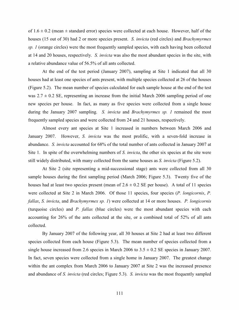
111

of 1.6 ± 0.2 (mean ± standard error) species were collected at each house. However, half of the

houses (15 out of 30) had 2 or more species present. S. invicta (red circles) and Brachymyrmex

sp. 1 (orange circles) were the most frequently sampled species, with each having been collected

at 14 and 20 houses, respectively. S. invicta was also the most abundant species in the site, with

a relative abundance value of 56.5% of all ants collected.

At the end of the test period (January 2007), sampling at Site 1 indicated that all 30

houses had at least one species of ants present, with multiple species collected at 26 of the houses

(Figure 5.2). The mean number of species calculated for each sample house at the end of the test

was 2.7 ± 0.2 SE, representing an increase from the initial March 2006 sampling period of one

new species per house. In fact, as many as five species were collected from a single house

during the January 2007 sampling. S. invicta and Brachymyrmex sp. 1 remained the most

frequently sampled species and were collected from 24 and 21 houses, respectively.

Almost every ant species at Site 1 increased in numbers between March 2006 and

January 2007. However, S. invicta was the most prolific, with a seven-fold increase in

abundance. S. invicta accounted for 68% of the total number of ants collected in January 2007 at

Site 1. In spite of the overwhelming numbers of S. invicta, the other six species at the site were

still widely distributed, with many collected from the same houses as S. invicta (Figure 5.2).

At Site 2 (site representing a mid-successional stage) ants were collected from all 30

sample houses during the first sampling period (March 2006; Figure 5.3). Twenty five of the

houses had at least two species present (mean of 2.6 ± 0.2 SE per house). A total of 11 species

were collected at Site 2 in March 2006. Of those 11 species, four species (P. longicornis, P.

fallax, S. invicta, and Brachymyrmex sp. 1) were collected at 14 or more houses. P. longicornis

(turquoise circles) and P. fallax (blue circles) were the most abundant species with each

accounting for 26% of the ants collected at the site, or a combined total of 52% of all ants

collected.

By January 2007 of the following year, all 30 houses at Site 2 had at least two different

species collected from each house (Figure 5.3). The mean number of species collected from a

single house increased from 2.6 species in March 2006 to 3.5 ± 0.2 SE species in January 2007.

In fact, seven species were collected from a single home in January 2007. The greatest change

within the ant complex from March 2006 to January 2007 at Site 2 was the increased presence

and abundance of S. invicta (red circles; Figure 5.3). S. invicta was the most frequently sampled

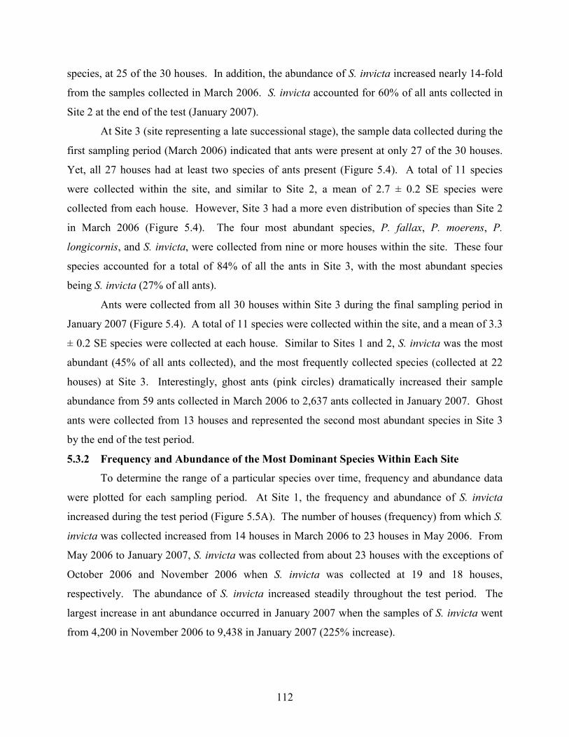
112

species, at 25 of the 30 houses. In addition, the abundance of S. invicta increased nearly 14-fold

from the samples collected in March 2006. S. invicta accounted for 60% of all ants collected in

Site 2 at the end of the test (January 2007).

At Site 3 (site representing a late successional stage), the sample data collected during the

first sampling period (March 2006) indicated that ants were present at only 27 of the 30 houses.

Yet, all 27 houses had at least two species of ants present (Figure 5.4). A total of 11 species

were collected within the site, and similar to Site 2, a mean of 2.7 ± 0.2 SE species were

collected from each house. However, Site 3 had a more even distribution of species than Site 2

in March 2006 (Figure 5.4). The four most abundant species, P. fallax, P. moerens, P.

longicornis, and S. invicta, were collected from nine or more houses within the site. These four

species accounted for a total of 84% of all the ants in Site 3, with the most abundant species

being S. invicta (27% of all ants).

Ants were collected from all 30 houses within Site 3 during the final sampling period in

January 2007 (Figure 5.4). A total of 11 species were collected within the site, and a mean of 3.3

± 0.2 SE species were collected at each house. Similar to Sites 1 and 2, S. invicta was the most

abundant (45% of all ants collected), and the most frequently collected species (collected at 22

houses) at Site 3. Interestingly, ghost ants (pink circles) dramatically increased their sample

abundance from 59 ants collected in March 2006 to 2,637 ants collected in January 2007. Ghost

ants were collected from 13 houses and represented the second most abundant species in Site 3

by the end of the test period.

5.3.2 Frequency and Abundance of the Most Dominant Species Within Each Site

To determine the range of a particular species over time, frequency and abundance data

were plotted for each sampling period. At Site 1, the frequency and abundance of S. invicta

increased during the test period (Figure 5.5A). The number of houses (frequency) from which S.

invicta was collected increased from 14 houses in March 2006 to 23 houses in May 2006. From

May 2006 to January 2007, S. invicta was collected from about 23 houses with the exceptions of

October 2006 and November 2006 when S. invicta was collected at 19 and 18 houses,

respectively. The abundance of S. invicta increased steadily throughout the test period. The

largest increase in ant abundance occurred in January 2007 when the samples of S. invicta went

from 4,200 in November 2006 to 9,438 in January 2007 (225% increase).

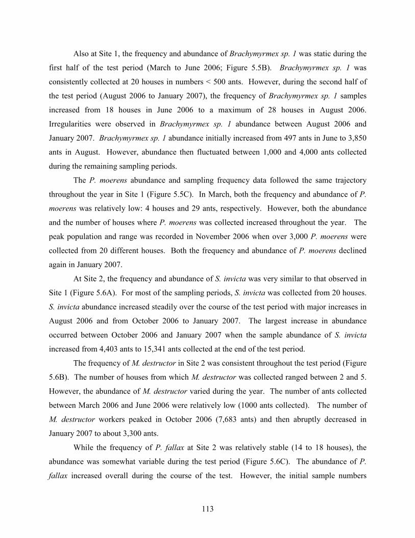
113

Also at Site 1, the frequency and abundance of Brachymyrmex sp. 1 was static during the

first half of the test period (March to June 2006; Figure 5.5B). Brachymyrmex sp. 1 was

consistently collected at 20 houses in numbers < 500 ants. However, during the second half of

the test period (August 2006 to January 2007), the frequency of Brachymyrmex sp. 1 samples

increased from 18 houses in June 2006 to a maximum of 28 houses in August 2006.

Irregularities were observed in Brachymyrmex sp. 1 abundance between August 2006 and

January 2007. Brachymyrmex sp. 1 abundance initially increased from 497 ants in June to 3,850

ants in August. However, abundance then fluctuated between 1,000 and 4,000 ants collected

during the remaining sampling periods.

The P. moerens abundance and sampling frequency data followed the same trajectory

throughout the year in Site 1 (Figure 5.5C). In March, both the frequency and abundance of P.

moerens was relatively low: 4 houses and 29 ants, respectively. However, both the abundance

and the number of houses where P. moerens was collected increased throughout the year. The

peak population and range was recorded in November 2006 when over 3,000 P. moerens were

collected from 20 different houses. Both the frequency and abundance of P. moerens declined

again in January 2007.

At Site 2, the frequency and abundance of S. invicta was very similar to that observed in

Site 1 (Figure 5.6A). For most of the sampling periods, S. invicta was collected from 20 houses.

S. invicta abundance increased steadily over the course of the test period with major increases in

August 2006 and from October 2006 to January 2007. The largest increase in abundance

occurred between October 2006 and January 2007 when the sample abundance of S. invicta

increased from 4,403 ants to 15,341 ants collected at the end of the test period.

The frequency of M. destructor in Site 2 was consistent throughout the test period (Figure

5.6B). The number of houses from which M. destructor was collected ranged between 2 and 5.

However, the abundance of M. destructor varied during the year. The number of ants collected

between March 2006 and June 2006 were relatively low (1000 ants collected). The number of

M. destructor workers peaked in October 2006 (7,683 ants) and then abruptly decreased in

January 2007 to about 3,300 ants.

While the frequency of P. fallax at Site 2 was relatively stable (14 to 18 houses), the

abundance was somewhat variable during the test period (Figure 5.6C). The abundance of P.

fallax increased overall during the course of the test. However, the initial sample numbers

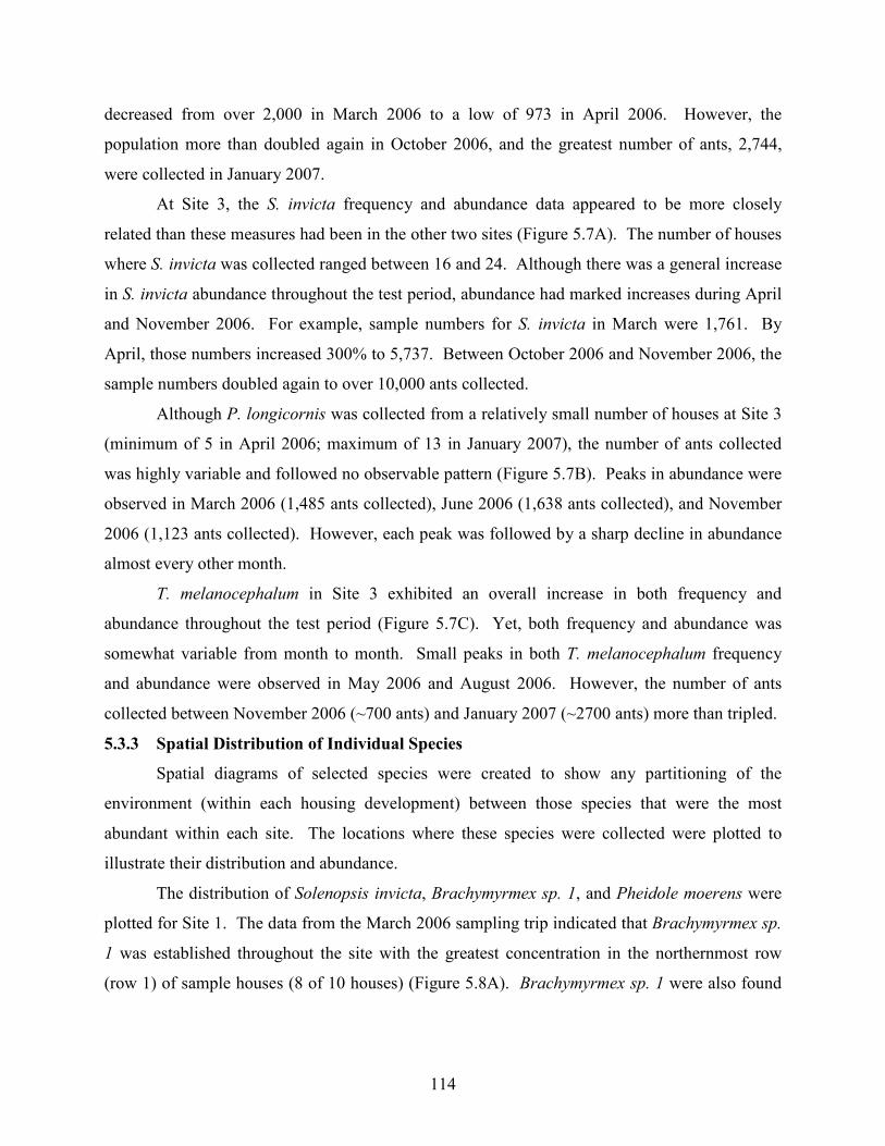
114

decreased from over 2,000 in March 2006 to a low of 973 in April 2006. However, the

population more than doubled again in October 2006, and the greatest number of ants, 2,744,

were collected in January 2007.

At Site 3, the S. invicta frequency and abundance data appeared to be more closely

related than these measures had been in the other two sites (Figure 5.7A). The number of houses

where S. invicta was collected ranged between 16 and 24. Although there was a general increase

in S. invicta abundance throughout the test period, abundance had marked increases during April

and November 2006. For example, sample numbers for S. invicta in March were 1,761. By

April, those numbers increased 300% to 5,737. Between October 2006 and November 2006, the

sample numbers doubled again to over 10,000 ants collected.

Although P. longicornis was collected from a relatively small number of houses at Site 3

(minimum of 5 in April 2006; maximum of 13 in January 2007), the number of ants collected

was highly variable and followed no observable pattern (Figure 5.7B). Peaks in abundance were

observed in March 2006 (1,485 ants collected), June 2006 (1,638 ants collected), and November

2006 (1,123 ants collected). However, each peak was followed by a sharp decline in abundance

almost every other month.

T. melanocephalum in Site 3 exhibited an overall increase in both frequency and

abundance throughout the test period (Figure 5.7C). Yet, both frequency and abundance was

somewhat variable from month to month. Small peaks in both T. melanocephalum frequency

and abundance were observed in May 2006 and August 2006. However, the number of ants

collected between November 2006 (~700 ants) and January 2007 (~2700 ants) more than tripled.

5.3.3 Spatial Distribution of Individual Species

Spatial diagrams of selected species were created to show any partitioning of the

environment (within each housing development) between those species that were the most

abundant within each site. The locations where these species were collected were plotted to

illustrate their distribution and abundance.

The distribution of Solenopsis invicta, Brachymyrmex sp. 1, and Pheidole moerens were

plotted for Site 1. The data from the March 2006 sampling trip indicated that Brachymyrmex sp.

1 was established throughout the site with the greatest concentration in the northernmost row

(row 1) of sample houses (8 of 10 houses) (Figure 5.8A). Brachymyrmex sp. 1 were also found

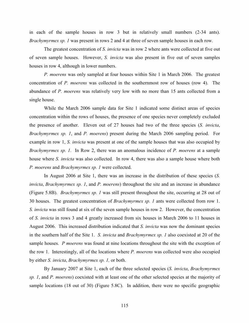
115

in each of the sample houses in row 3 but in relatively small numbers (2-34 ants).

Brachymyrmex sp. 1 was present in rows 2 and 4 at three of seven sample houses in each row.

The greatest concentration of S. invicta was in row 2 where ants were collected at five out

of seven sample houses. However, S. invicta was also present in five out of seven samples

houses in row 4, although in lower numbers.

P. moerens was only sampled at four houses within Site 1 in March 2006. The greatest

concentration of P. moerens was collected in the southernmost row of houses (row 4). The

abundance of P. moerens was relatively very low with no more than 15 ants collected from a

single house.

While the March 2006 sample data for Site 1 indicated some distinct areas of species

concentration within the rows of houses, the presence of one species never completely excluded

the presence of another. Eleven out of 27 houses had two of the three species (S. invicta,

Brachymyrmex sp. 1, and P. moerens) present during the March 2006 sampling period. For

example in row 1, S. invicta was present at one of the sample houses that was also occupied by

Brachymyrmex sp. 1. In Row 2, there was an anomalous incidence of P. moerens at a sample

house where S. invicta was also collected. In row 4, there was also a sample house where both

P. moerens and Brachymyrmex sp. 1 were collected.

In August 2006 at Site 1, there was an increase in the distribution of these species (S.

invicta, Brachymyrmex sp. 1, and P. moerens) throughout the site and an increase in abundance

(Figure 5.8B). Brachymyrmex sp. 1 was still present throughout the site, occurring at 28 out of

30 houses. The greatest concentration of Brachymyrmex sp. 1 ants were collected from row 1.

S. invicta was still found at six of the seven sample houses in row 2. However, the concentration

of S. invicta in rows 3 and 4 greatly increased from six houses in March 2006 to 11 houses in

August 2006. This increased distribution indicated that S. invicta was now the dominant species

in the southern half of the Site 1. S. invicta and Brachymyrmex sp. 1 also coexisted at 20 of the

sample houses. P moerens was found at nine locations throughout the site with the exception of

the row 1. Interestingly, all of the locations where P. moerens was collected were also occupied

by either S. invicta, Brachymyrmex sp. 1, or both.

By January 2007 at Site 1, each of the three selected species (S. invicta, Brachymyrmex

sp. 1, and P. moerens) coexisted with at least one of the other selected species at the majority of

sample locations (18 out of 30) (Figure 5.8C). In addition, there were no specific geographic

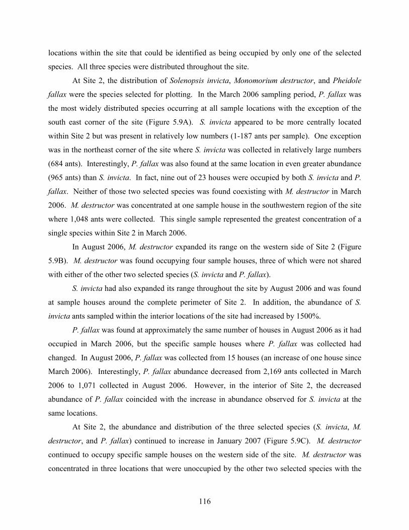
116

locations within the site that could be identified as being occupied by only one of the selected

species. All three species were distributed throughout the site.

At Site 2, the distribution of Solenopsis invicta, Monomorium destructor, and Pheidole

fallax were the species selected for plotting. In the March 2006 sampling period, P. fallax was

the most widely distributed species occurring at all sample locations with the exception of the

south east corner of the site (Figure 5.9A). S. invicta appeared to be more centrally located

within Site 2 but was present in relatively low numbers (1-187 ants per sample). One exception

was in the northeast corner of the site where S. invicta was collected in relatively large numbers

(684 ants). Interestingly, P. fallax was also found at the same location in even greater abundance

(965 ants) than S. invicta. In fact, nine out of 23 houses were occupied by both S. invicta and P.

fallax. Neither of those two selected species was found coexisting with M. destructor in March

2006. M. destructor was concentrated at one sample house in the southwestern region of the site

where 1,048 ants were collected. This single sample represented the greatest concentration of a

single species within Site 2 in March 2006.

In August 2006, M. destructor expanded its range on the western side of Site 2 (Figure

5.9B). M. destructor was found occupying four sample houses, three of which were not shared

with either of the other two selected species (S. invicta and P. fallax).

S. invicta had also expanded its range throughout the site by August 2006 and was found

at sample houses around the complete perimeter of Site 2. In addition, the abundance of S.

invicta ants sampled within the interior locations of the site had increased by 1500%.

P. fallax was found at approximately the same number of houses in August 2006 as it had

occupied in March 2006, but the specific sample houses where P. fallax was collected had

changed. In August 2006, P. fallax was collected from 15 houses (an increase of one house since

March 2006). Interestingly, P. fallax abundance decreased from 2,169 ants collected in March

2006 to 1,071 collected in August 2006. However, in the interior of Site 2, the decreased

abundance of P. fallax coincided with the increase in abundance observed for S. invicta at the

same locations.

At Site 2, the abundance and distribution of the three selected species (S. invicta, M.

destructor, and P. fallax) continued to increase in January 2007 (Figure 5.9C). M. destructor

continued to occupy specific sample houses on the western side of the site. M. destructor was

concentrated in three locations that were unoccupied by the other two selected species with the

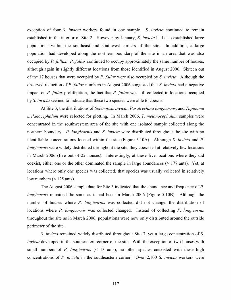
117

exception of four S. invicta workers found in one sample. S. invicta continued to remain

established in the interior of Site 2. However by January, S. invicta had also established large

populations within the southeast and southwest corners of the site. In addition, a large

population had developed along the northern boundary of the site in an area that was also

occupied by P. fallax. P. fallax continued to occupy approximately the same number of houses,

although again in slightly different locations from those identified in August 2006. Sixteen out

of the 17 houses that were occupied by P. fallax were also occupied by S. invicta. Although the

observed reduction of P. fallax numbers in August 2006 suggested that S. invicta had a negative

impact on P. fallax proliferation, the fact that P. fallax was still collected in locations occupied

by S. invicta seemed to indicate that these two species were able to coexist.

At Site 3, the distributions of Solenopsis invicta, Paratrechina longicornis, and Tapinoma

melanocephalum were selected for plotting. In March 2006, T. melanocephalum samples were

concentrated in the southwestern area of the site with one isolated sample collected along the

northern boundary. P. longicornis and S. invicta were distributed throughout the site with no

identifiable concentrations located within the site (Figure 5.10A). Although S. invicta and P.

longicornis were widely distributed throughout the site, they coexisted at relatively few locations

in March 2006 (five out of 22 houses). Interestingly, at these five locations where they did

coexist, either one or the other dominated the sample in large abundances (> 177 ants). Yet, at

locations where only one species was collected, that species was usually collected in relatively

low numbers (< 125 ants).

The August 2006 sample data for Site 3 indicated that the abundance and frequency of P.

longicornis remained the same as it had been in March 2006 (Figure 5.10B). Although the

number of houses where P. longicornis was collected did not change, the distribution of

locations where P. longicornis was collected changed. Instead of collecting P. longicornis

throughout the site as in March 2006, populations were now only distributed around the outside

perimeter of the site.

S. invicta remained widely distributed throughout Site 3, yet a large concentration of S.

invicta developed in the southeastern corner of the site. With the exception of two houses with

small numbers of P. longicornis (< 13 ants), no other species coexisted with these high

concentrations of S. invicta in the southeastern corner. Over 2,100 S. invicta workers were

118

collected from a single sample house in the southeastern corner, representing the greatest number

of ants collected from a single house during the entire test period.

The abundance and distribution of T. melanocephalum at Site 3 also increased from

March 2006 to August 2006. T. melanocephalum was collected throughout the site with the

exception of the southeastern corner where high numbers of S. invicta were found. Overall, at

least two of the three selected species coexisted at half of the sample houses (14 out of 28).

However, most of these 14 houses were located along the perimeter of the site.

The January 2007 sample data for Site 3 indicated that all three species (S. invicta, P.

longicornis, and T. melanocephalum) were distributed throughout the site (Figure 5.10C).

Although the abundance of P. longicornis decreased by almost half (since August 2006), this

species was collected from a greater number of houses (13 houses) within the site. T.

melanocephalum continued to be widely distributed throughout Site 3, even where high

concentrations of S. invicta were also present. S. invicta also continued to be widely distributed

throughout the site, and still maintained a large concentration in the southeastern section of Site

3. Additional large concentrations of S. invicta were also collected from sample houses in the

southwestern and northern regions of the site. At those houses where large numbers of S. invicta

were collected (in the southwestern, southeastern, and northern locations), samples of either P.

longicornis or T. melanocephalum were also collected. In fact, by January 2007, over 70% of

the sample houses (19 out of 27) had two or more species coexisting. However, T.

melanocephalum and P. longicornis were rarely collected at the same sample house (2 out of

30).

5.4 Discussion

5.4.1 Distribution and Abundance Diagrams of Ant Species

The presence or absence of ant species at the bait samples provided information about the

foraging ranges of the different species and the plasticity of their territorial boundaries

throughout the year. The results of this study indicated that multiple ant species were able to

establish populations very quickly in a disturbed urban habitat. Yet, these populations were not

static in their distribution. In fact, the foraging range of the dominant species expanded over the

course of the year resulting in a greater overlap of foraging territories than had been anticipated.

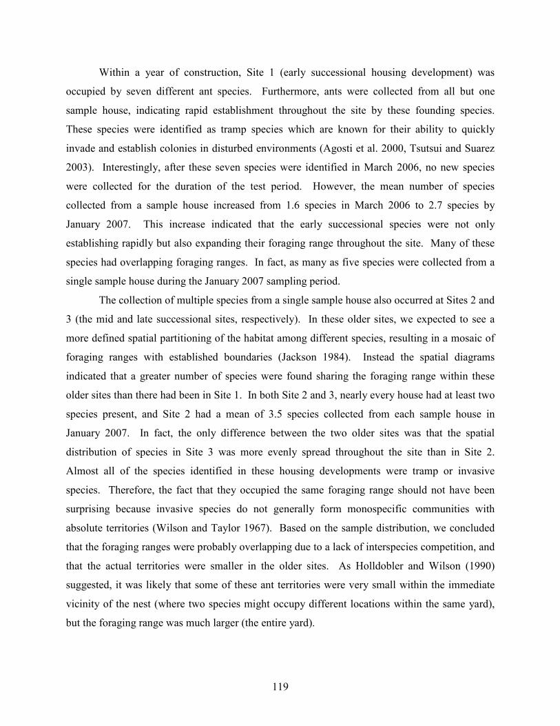
119

Within a year of construction, Site 1 (early successional housing development) was

occupied by seven different ant species. Furthermore, ants were collected from all but one

sample house, indicating rapid establishment throughout the site by these founding species.

These species were identified as tramp species which are known for their ability to quickly

invade and establish colonies in disturbed environments (Agosti et al. 2000, Tsutsui and Suarez

2003). Interestingly, after these seven species were identified in March 2006, no new species

were collected for the duration of the test period. However, the mean number of species

collected from a sample house increased from 1.6 species in March 2006 to 2.7 species by

January 2007. This increase indicated that the early successional species were not only

establishing rapidly but also expanding their foraging range throughout the site. Many of these

species had overlapping foraging ranges. In fact, as many as five species were collected from a

single sample house during the January 2007 sampling period.

The collection of multiple species from a single sample house also occurred at Sites 2 and

3 (the mid and late successional sites, respectively). In these older sites, we expected to see a

more defined spatial partitioning of the habitat among different species, resulting in a mosaic of

foraging ranges with established boundaries (Jackson 1984). Instead the spatial diagrams

indicated that a greater number of species were found sharing the foraging range within these

older sites than there had been in Site 1. In both Site 2 and 3, nearly every house had at least two

species present, and Site 2 had a mean of 3.5 species collected from each sample house in

January 2007. In fact, the only difference between the two older sites was that the spatial

distribution of species in Site 3 was more evenly spread throughout the site than in Site 2.

Almost all of the species identified in these housing developments were tramp or invasive

species. Therefore, the fact that they occupied the same foraging range should not have been

surprising because invasive species do not generally form monospecific communities with

absolute territories (Wilson and Taylor 1967). Based on the sample distribution, we concluded

that the foraging ranges were probably overlapping due to a lack of interspecies competition, and

that the actual territories were smaller in the older sites. As Holldobler and Wilson (1990)

suggested, it was likely that some of these ant territories were very small within the immediate

vicinity of the nest (where two species might occupy different locations within the same yard),

but the foraging range was much larger (the entire yard).

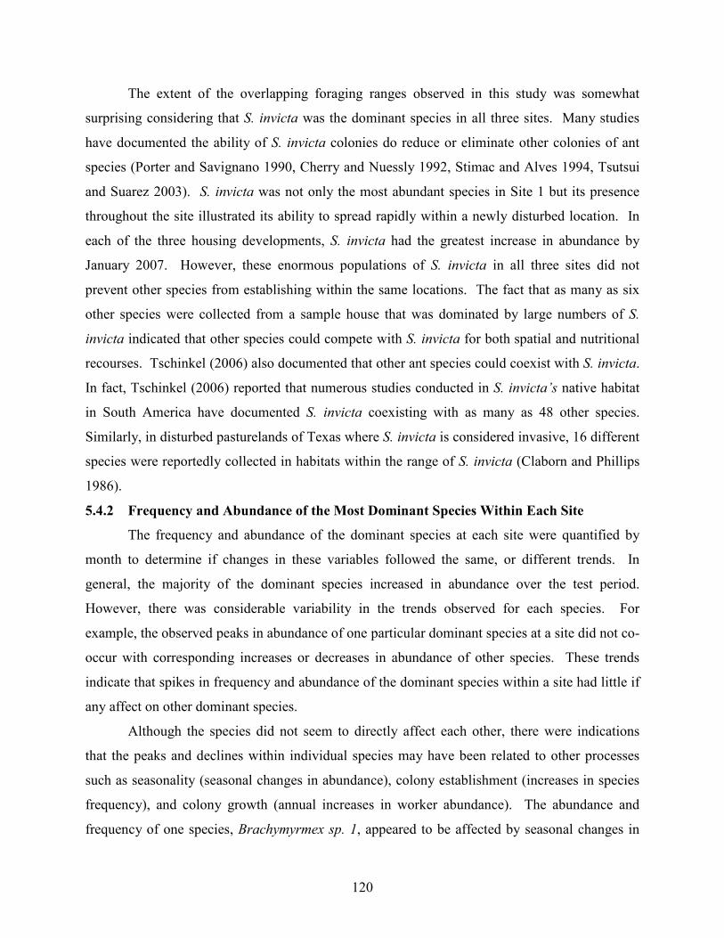
120

The extent of the overlapping foraging ranges observed in this study was somewhat

surprising considering that S. invicta was the dominant species in all three sites. Many studies

have documented the ability of S. invicta colonies do reduce or eliminate other colonies of ant

species (Porter and Savignano 1990, Cherry and Nuessly 1992, Stimac and Alves 1994, Tsutsui

and Suarez 2003). S. invicta was not only the most abundant species in Site 1 but its presence

throughout the site illustrated its ability to spread rapidly within a newly disturbed location. In

each of the three housing developments, S. invicta had the greatest increase in abundance by

January 2007. However, these enormous populations of S. invicta in all three sites did not

prevent other species from establishing within the same locations. The fact that as many as six

other species were collected from a sample house that was dominated by large numbers of S.

invicta indicated that other species could compete with S. invicta for both spatial and nutritional

recourses. Tschinkel (2006) also documented that other ant species could coexist with S. invicta.

In fact, Tschinkel (2006) reported that numerous studies conducted in S. invicta’s native habitat

in South America have documented S. invicta coexisting with as many as 48 other species.

Similarly, in disturbed pasturelands of Texas where S. invicta is considered invasive, 16 different

species were reportedly collected in habitats within the range of S. invicta (Claborn and Phillips

1986).

5.4.2 Frequency and Abundance of the Most Dominant Species Within Each Site

The frequency and abundance of the dominant species at each site were quantified by

month to determine if changes in these variables followed the same, or different trends. In

general, the majority of the dominant species increased in abundance over the test period.

However, there was considerable variability in the trends observed for each species. For

example, the observed peaks in abundance of one particular dominant species at a site did not co-

occur with corresponding increases or decreases in abundance of other species. These trends

indicate that spikes in frequency and abundance of the dominant species within a site had little if

any affect on other dominant species.

Although the species did not seem to directly affect each other, there were indications

that the peaks and declines within individual species may have been related to other processes

such as seasonality (seasonal changes in abundance), colony establishment (increases in species

frequency), and colony growth (annual increases in worker abundance). The abundance and

frequency of one species, Brachymyrmex sp. 1, appeared to be affected by seasonal changes in

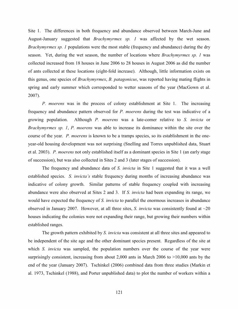
121

Site 1. The differences in both frequency and abundance observed between March-June and

August-January suggested that Brachymyrmex sp. 1 was affected by the wet season.

Brachymyrmex sp. 1 populations were the most stable (frequency and abundance) during the dry

season. Yet, during the wet season, the number of locations where Brachymyrmex sp. 1 was

collected increased from 18 houses in June 2006 to 28 houses in August 2006 as did the number

of ants collected at these locations (eight-fold increase). Although, little information exists on

this genus, one species of Brachymyrmex, B. patagonicus, was reported having mating flights in

spring and early summer which corresponded to wetter seasons of the year (MacGown et al.

2007).

P. moerens was in the process of colony establishment at Site 1. The increasing

frequency and abundance pattern observed for P. moerens during the test was indicative of a

growing population. Although P. moerens was a late-comer relative to S. invicta or

Brachymyrmex sp. 1, P. moerens was able to increase its dominance within the site over the

course of the year. P. moerens is known to be a tramps species, so its establishment in the one-

year-old housing development was not surprising (Snelling and Torres unpublished data, Stuart

et al. 2003). P. moerens not only established itself as a dominant species in Site 1 (an early stage

of succession), but was also collected in Sites 2 and 3 (later stages of succession).

The frequency and abundance data of S. invicta in Site 1 suggested that it was a well

established species. S. invicta’s stable frequency during months of increasing abundance was

indicative of colony growth. Similar patterns of stable frequency coupled with increasing

abundance were also observed at Sites 2 and 3. If S. invicta had been expanding its range, we

would have expected the frequency of S. invicta to parallel the enormous increases in abundance

observed in January 2007. However, at all three sites, S. invicta was consistently found at ~20

houses indicating the colonies were not expanding their range, but growing their numbers within

established ranges.

The growth pattern exhibited by S. invicta was consistent at all three sites and appeared to

be independent of the site age and the other dominant species present. Regardless of the site at

which S. invicta was sampled, the population numbers over the course of the year were

surprisingly consistent, increasing from about 2,000 ants in March 2006 to >10,000 ants by the

end of the year (January 2007). Tschinkel (2006) combined data from three studies (Markin et

al. 1973, Tschinkel (1988), and Porter unpublished data) to plot the number of workers within a

122

fire ant colony by the age of the colony. Tschinkel (2006) then fitted a curve to those data and

found that fire ant colony growth fluctuated on an annual cycle. At the beginning of the year, the

number of workers would be relatively low. The number of workers would then increase over

the year to a peak, and then decrease back to numbers similar to those observed at the beginning

of the year. Although we did not record a full annual cycle in Puerto Rico, the curve recorded by

Tschinkel (2006) fits closely with our data from March 2006 to January 2007. Therefore, we

concluded that within each site, the populations of S. invicta that we observed in January 2007,

would shrink back to the initial levels recorded at the beginning of the test in March 2006.

The other dominant species at Sites 2 and 3 (P. fallax, M. destructor, P. longicornis, and

T. melanocephalum) also had relatively stable frequencies but variable abundance data, which

suggested that these species also had annual population cycle. P. fallax at Site 2 and T.

melanocephalum at Site 3 both had annual population cycles in which there was a general

increase in abundance during the test period. Unfortunately, detailed information on the colony

life cycle of either P. fallax or T. melanocephalum does not exist in the current literature. Our

data indicate that P. fallax and T. melanocephalum, like S. invicta, experienced colony growth

throughout the wet season (November). However, worker populations would be expected to

decrease with the onset of the dry season. We also hypothesize that a peak in the abundance of

M. destructor also occurred in conjunction with the wet season. This early peak in October 2006

(relative to later peaks of S. invicta and P. fallax in January 2007) may have allowed it to avoid

competition with the other dominant species at Site 2.

P. longicornis experienced two peaks in abundance in March 2006 and then again in June

2006. While the March 2006 peak was difficult to explain, the June 2006 peak was very likely

related to alate production. Trager (1984) reported that the alate production of P. longicornis

occurred between May and September during warm rainy months in northern Florida. Although

May is usually a drier month of the year, June marks the beginning of hurricane season in Puerto

Rico. Therefore, the peak in abundance corresponded to seasonal conditions in Santa Isabel that

were favorable to the production of alates and colony growth.

Interestingly, at the older sites, the abundance peaks of the dominant species did not co-

occur with similar increases in the frequency of those species. Therefore, these dominant species

were likely producing large numbers of workers from well established colonies instead of

expanding their range to new houses.

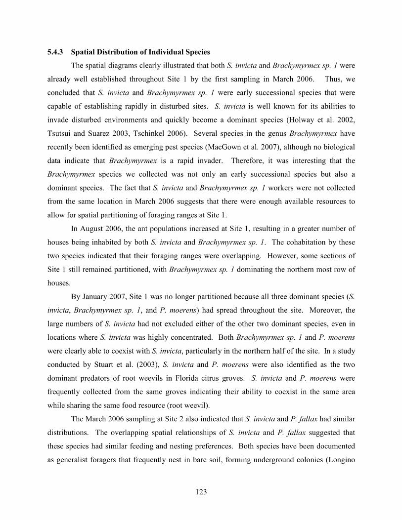
123

5.4.3 Spatial Distribution of Individual Species

The spatial diagrams clearly illustrated that both S. invicta and Brachymyrmex sp. 1 were

already well established throughout Site 1 by the first sampling in March 2006. Thus, we

concluded that S. invicta and Brachymyrmex sp. 1 were early successional species that were

capable of establishing rapidly in disturbed sites. S. invicta is well known for its abilities to

invade disturbed environments and quickly become a dominant species (Holway et al. 2002,

Tsutsui and Suarez 2003, Tschinkel 2006). Several species in the genus Brachymyrmex have

recently been identified as emerging pest species (MacGown et al. 2007), although no biological

data indicate that Brachymyrmex is a rapid invader. Therefore, it was interesting that the

Brachymyrmex species we collected was not only an early successional species but also a

dominant species. The fact that S. invicta and Brachymyrmex sp. 1 workers were not collected

from the same location in March 2006 suggests that there were enough available resources to

allow for spatial partitioning of foraging ranges at Site 1.

In August 2006, the ant populations increased at Site 1, resulting in a greater number of

houses being inhabited by both S. invicta and Brachymyrmex sp. 1. The cohabitation by these

two species indicated that their foraging ranges were overlapping. However, some sections of

Site 1 still remained partitioned, with Brachymyrmex sp. 1 dominating the northern most row of

houses.

By January 2007, Site 1 was no longer partitioned because all three dominant species (S.

invicta, Brachymyrmex sp. 1, and P. moerens) had spread throughout the site. Moreover, the

large numbers of S. invicta had not excluded either of the other two dominant species, even in

locations where S. invicta was highly concentrated. Both Brachymyrmex sp. 1 and P. moerens

were clearly able to coexist with S. invicta, particularly in the northern half of the site. In a study

conducted by Stuart et al. (2003), S. invicta and P. moerens were also identified as the two

dominant predators of root weevils in Florida citrus groves. S. invicta and P. moerens were

frequently collected from the same groves indicating their ability to coexist in the same area

while sharing the same food resource (root weevil).

The March 2006 sampling at Site 2 also indicated that S. invicta and P. fallax had similar

distributions. The overlapping spatial relationships of S. invicta and P. fallax suggested that

these species had similar feeding and nesting preferences. Both species have been documented

as generalist foragers that frequently nest in bare soil, forming underground colonies (Longino

124

and Cover 1997, Tschinkel 2006). The distribution of these two species did not change in either

August 2006 or January 2007, indicating that colony locations were well established and that

Site 2 was a more stable community than Site 1.

By August 2006, both P. fallax and S. invicta had increased their frequency in Site 2.

However, locations where S. invicta was collected had greater concentrations of workers than P.

fallax. No doubt this was due to the prolific nature of S. invicta (Tschinkel 2006). We speculate

that the tremendous numbers of S. invicta were able to out compete P. fallax for available

resources, and therefore limited P. fallax’s foraging range and numbers. The competition

between S. invicta and P. fallax may have resulted in spatial partitioning of the site with high

abundances of S. invicta observed in the center of the site while the greater abundances of P.

fallax were pushed the perimeter of Site 2.

In January 2007, P. fallax was collected at several locations where S. invicta was

established. Although S. invicta remained the most prolific of the two species, the continued

presence of P. fallax indicated that P. fallax was able to coexist and compete, to some degree,

with the more dominant S. invicta. While there is limited biological information in the scientific

literature regarding P. fallax, other species of Pheidole, specifically tramp species (P.

megacephala, P. moerens) have been documented coexisting with S. invicta (Stuart et al. 2003,

Tschinkel 2006). We hypothesize that P. fallax may defend small territories, possibly smaller

than our spatial diagrams can detect. Yet, P. fallax was able to sustain their colonies while

continuing to forage in ranges shared with S. invicta.

Although the majority of Site 2 was dominated by overlapping foraging ranges of S.

invicta and P. fallax, M. destructor maintained a relatively exclusive position in the southwestern

corner of Site 2. The absence of S. invicta in this location indicated that M. destructor was

capable of maintaining foraging boundaries that prevented the invasion of S. invicta. M.

destructor’s dominance of the southwestern region in Site 2 did not change over the test period,

and M. destructor appeared to be able to defend its foraging boundaries, with only a few rare

appearances by other species. Although M. destructor was dominant in one corner of the site,

this species did not expand its initial range beyond a few sample houses. M. destructor has been

identified as a tramp species that only inhabits urban environments. This species is polygyne and

has been documented in Australia and South Pacific islands as having such large numbers of

workers as to give the appearance of being a super colony. Harris (2005a) has determined that

125

M. destructor’s presence has led to a decrease in native ant species, and that it was a threat to

biodiversity. This ability to reduce or eliminate competitors may explain why few species were

found within M. destructor’s foraging range in Site 2. However, M. destructor does not recruit

to food sources as rapidly as other tramp species which may explain its limited distribution in

Site 2 where many other tramp ant species were present (Harris 2005a).

At Site 3, there were relatively few locations where the different dominant species

coexisted together in large numbers. Thus, the spatial diagrams indicated more spatial

partitioning in Site 3 than was observed in the other two sites. For example, P. longicornis and

S. invicta were rarely found to overlap in large numbers in March 2006 or August 2006. The

reason for this spatial separation may be partially attributed to P. longicornis and S. invicta

having different feeding and nesting preferences (Smith 1965). P. longicornis is a sweet feeding

ant that frequently relocates its nest. It also tends to nest in man-made harborages. S. invicta is a

generalist feeder that builds extensive nests in the soil (Smith 1965). These species were

collected at different houses most likely because the nesting locations were more conducive for

one species or the other to establish. For example, P. longicornis was frequently collected at

houses with overgrown yards and those yards littered with human debris. S. invicta was

frequently collected from barren yards lacking any landscaping or even grass. Only in January

2007 when T. melanocephalum spread throughout the site, were large concentrations of S. invicta

and P. longicornis frequently collected at the same location. The coexistence of S. invicta and P.

longicornis suggested that while these two species preferred to live in separate locations, both

species could coexist together if necessary.

The third species we observed at Site 3, T. melanocephalum, initially appeared to be only

a minor species. In March 2006, T. melanocephalum occurred only at a few locations and in

small numbers. Yet, as the year progressed, T. melanocephalum spread throughout the site and

became a dominant species. At many locations, T. melanocephalum coexisted with large

populations of S. invicta. Interestingly, in January 2007, T. melanocephalum was the only

species collected in some locations that had previously been occupied by S. invicta and/or P.

longicornis in August 2006. The absence of S. invicta and P. longicornis from these sample

houses in January 2007 suggested that T. melanocephalum was excluding the other dominant

species. The absence of T. melanocephalum in Sites 1 and 2, and its rapid, aggressive expansion

126

throughout Site 3 suggested that T. melanocephalum was a dominant, yet late successional

species.

Our findings were contrary to the current literature regarding T. melanocephalum.

However, most studies regarding T. melanocephalum were conducted in disturbed natural

environments where the land was cleared for agriculture (i.e. rice fields and banana plantations;

Harris 2005b). In these disturbed natural locations, T. melanocephalum has not been found to be

a numerically or behaviorally dominant species. Harris (2005b) reported that in disturbed natural

environments, the displacement of other ant species by T. melanocephalum was unlikely.

However, based on our data in disturbed urban environments, T. melanocephalum appeared to be

more dominant than these previous studies suggest.

T. melanocephalum was also found to have a unique interaction with P. longicornis. In

all three spatial diagrams for Site 3, the coexistence of T. melanocephalum and P. longicornis

was rarely observed. Because both species have similar foraging styles and feeding preferences

(i.e. rapid recruitment to food sources with a preference for sweet foods; Smith 1965), we

concluded that these two species were exhibiting spatial partitioning.

Further evidence of this interspecific competition was observed in January 2007 when T.

melanocephalum numbers reached peak abundance, while P. longicornis experienced a decrease

in abundance. While S. invicta might have been responsible for the decline of P. longicornis

numbers, we would have expected S. invicta to cause a similar decline in T. melanocephalum,

because T. melanocephalum and P. longicornis have similar feeding and foraging habits (Smith

1965). However, this was not the case. S. invicta and T. melanocephalum not only coexisted,

but both species were collected in high numbers from the same sample houses in January 2007.

Therefore, we concluded that the decline in P. longicornis was in fact due to the greater numbers

of T. melanocephalum out competing P. longicornis for resources.

5.4.4 Conclusions

The spatial diagrams indicated that as urban housing developments proceeded through

the stages of succession, more species of foraging ants were found cohabitating together. Clearly

these species were not supporting the ant mosaic hypothesis (Jackson 1984, Adams 1994) but

instead appeared to have spatially arranged themselves in a “scatter plot” distribution. In the ant

“scatter plot” distribution, territories appeared to be small or not defined at all. Even the

dominant species were not excluding other species from inhabiting locations where dominant

127

species were established. Interestingly, in all three sites, the coexistence of multiple species

increased throughout the test period. The low abundances of established species early in the year

promoted spatial partitioning and reduced the overlap of species’ foraging ranges. Yet as the

year progressed, less partitioning and a greater occurrence of coexistence indicated that annual

colony growth had a greater affect on species territoriality (spatial partitioning was reduced) than

did the successional stage of the environment.

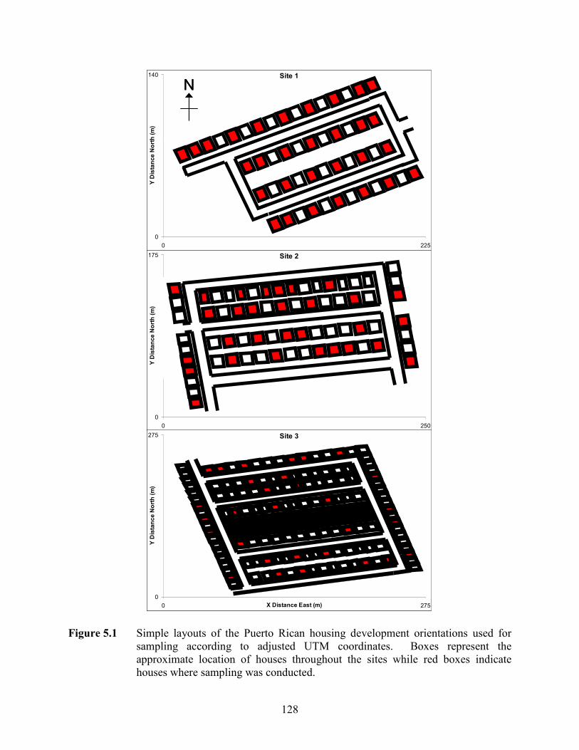
128

Site 1

0

140

0 225

Y Distance North (m)

Site 2

0

175

0 250


Site 3

0

275

0 275X Distance East (m)


NSite 1

0

140

0 225


Site 2

0

175

0 250


Site 3

0

275



Site 1

0

140

0 225


Site 2

0

175

0 250


Site 3

0

275



NN

Figure 5.1 Simple layouts of the Puerto Rican housing development orientations used for

sampling according to adjusted UTM coordinates. Boxes represent the approximate location of houses throughout the sites while red boxes indicate houses where sampling was conducted.

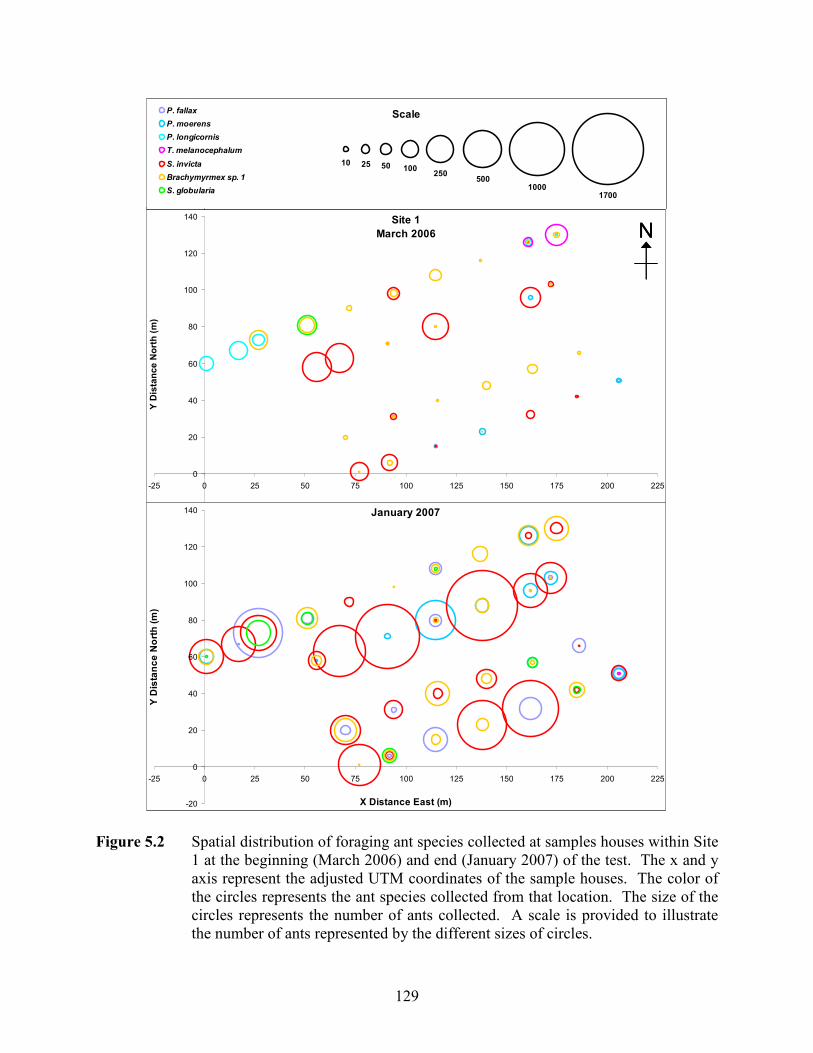
129

Scale

10 25 50 100250

5001000

1700

130

180


Site 1

March 2006

-20

0

20

40

60

80

100

120

140

-25 0 25 50 75 100 125 150 175 200 225


N

January 2007

-20

0

20

40

60

80

100

120

140

-25 0 25 50 75 100 125 150 175 200 225

X Distance East (m)


P. fallax

P. moerens

P. longicornis

T. melanocephalum

S. invicta

Brachymyrmex sp. 1

S. globularia

Scale

10 25 50 100250

5001000

1700

130

180


Site 1

March 2006

-20

0

20

40

60

80

100

120

140

-25 0 25 50 75 100 125 150 175 200 225


NN

January 2007

-20

0

20

40

60

80

100

120

140

-25 0 25 50 75 100 125 150 175 200 225

X Distance East (m)


P. fallax

P. moerens

P. longicornis

T. melanocephalum

S. invicta

Brachymyrmex sp. 1

S. globularia

Figure 5.2 Spatial distribution of foraging ant species collected at samples houses within Site

1 at the beginning (March 2006) and end (January 2007) of the test. The x and y axis represent the adjusted UTM coordinates of the sample houses. The color of the circles represents the ant species collected from that location. The size of the circles represents the number of ants collected. A scale is provided to illustrate the number of ants represented by the different sizes of circles.

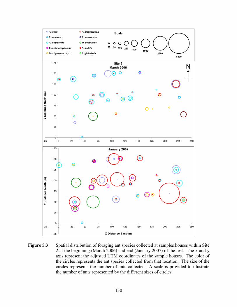
130

Scale

25 50 100 250 5001000

2500

5400150

175

200

225

Site 2

March 2006

-25

0

25

50

75

100

125

150

175

-25 0 25 50 75 100 125 150 175 200 225 250


N

January 2007

-25

0

25

50

75

100

125

150

175

-25 0 25 50 75 100 125 150 175 200 225 250

X Distance East (m)


P. fallax P. megacephala

P. moerens P. subarmata

P. longicornis M. destructor

T. melanocephalum S. invicta

Brachymyrmex sp. 1 S. globularia

Scale

25 50 100 250 5001000

2500

5400150

175

200

225

Site 2

March 2006

-25

0

25

50

75

100

125

150

175

-25 0 25 50 75 100 125 150 175 200 225 250


NN

January 2007

-25

0

25

50

75

100

125

150

175

-25 0 25 50 75 100 125 150 175 200 225 250

X Distance East (m)









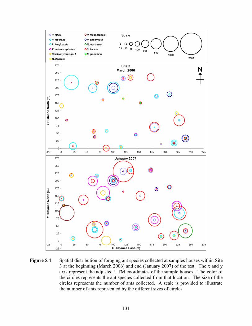
131

Site 3

March 2006

-25

0

25

50

75

100

125

150

175

200

225

250

275

-25 0 25 50 75 100 125 150 175 200 225 250 275


N

January 2007

-25

0

25

50

75

100

125

150

175

200

225

250

275

-25 0 25 50 75 100 125 150 175 200 225 250 275

X Distance East (m)


Scale

10 25 50 100250

5001000

2000






M. floricola

Site 3

March 2006

-25

0

25

50

75

100

125

150

175

200

225

250

275

-25 0 25 50 75 100 125 150 175 200 225 250 275


NN

January 2007

-25

0

25

50

75

100

125

150

175

200

225

250

275

-25 0 25 50 75 100 125 150 175 200 225 250 275

X Distance East (m)


Scale

10 25 50 100250

5001000

2000






M. floricola



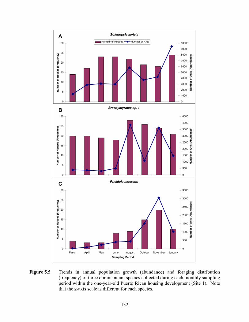
132

Solenopsis invicta

0

5

10

15

20

25

30

March April May June August October November January

Sampling Period

Number of Houses (Frequency)

0

1000

2000

3000

4000

5000

6000

7000

8000

9000

10000

Number of Ants (Abundance)

Number of Houses Number of Ants

Brachymyrmex sp. 1

0

5

10

15

20

25

30


Sampling Period


0

500

1000

1500

2000

2500

3000

3500

4000

4500


Pheidole moerens

0

5

10

15

20

25

30


Sampling Period


0

500

1000

1500

2000

2500

3000

3500Number of Ants (Abundance)

A

B

C

Solenopsis invicta

0

5

10

15

20

25

30


Sampling Period


0

1000

2000

3000

4000

5000

6000

7000

8000

9000

10000



Brachymyrmex sp. 1

0

5

10

15

20

25

30


Sampling Period


0

500

1000

1500

2000

2500

3000

3500

4000

4500


Pheidole moerens

0

5

10

15

20

25

30


Sampling Period


0

500

1000

1500

2000

2500

3000


A

B

C


(frequency) of three dominant ant species collected during each monthly sampling period within the one-year-old Puerto Rican housing development (Site 1). Note that the z-axis scale is different for each species.

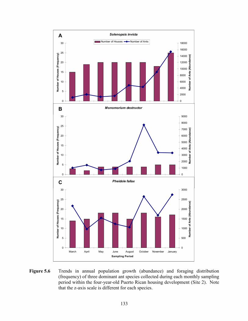
133

Solenopsis invicta

0

5

10

15

20

25

30


Month of Sampling Period


0

2000

4000

6000

8000

10000

12000

14000

16000

18000




0

5

10

15

20

25

30




0

1000

2000

3000

4000

5000

6000

7000

8000

9000


Pheidole fallax

0

5

10

15

20

25

30


Sampling Period


0

500

1000

1500

2000

2500


A

C

B

Solenopsis invicta

0

5

10

15

20

25

30




0

2000

4000

6000

8000

10000

12000

14000

16000

18000




0

5

10

15

20

25

30




0

1000

2000

3000

4000

5000

6000

7000

8000

9000


Pheidole fallax

0

5

10

15

20

25

30


Sampling Period


0

500

1000

1500

2000

2500


A

C

B

Figure 5.6 Trends in annual population growth (abundance) and foraging distribution (frequency) of three dominant ant species collected during each monthly sampling period within the four-year-old Puerto Rican housing development (Site 2). Note that the z-axis scale is different for each species.

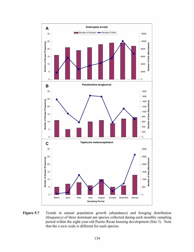
134

Solenopsis invicta

0

5

10

15

20

25

30




0

2000

4000

6000

8000

10000

12000




0

5

10

15

20

25

30




0

200

400

600

800

1000

1200

1400

1600

1800



0

5

10

15

20

25

30


Sampling Period


0

500

1000

1500

2000

2500


A

C

B

Solenopsis invicta

0

5

10

15

20

25

30




0

2000

4000

6000

8000

10000

12000




0

5

10

15

20

25

30




0

200

400

600

800

1000

1200

1400

1600

1800



0

5

10

15

20

25

30


Sampling Period


0

500

1000

1500

2000

2500


A

C

B


(frequency) of three dominant ant species collected during each monthly sampling period within the eight-year-old Puerto Rican housing development (Site 3). Note that the z-axis scale is different for each species.

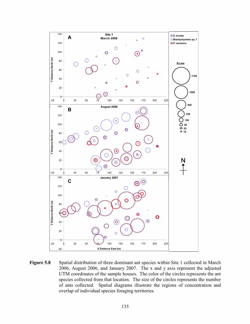
135

N

Scale

10

25

50

100

250

500

1000

1700

Site 1

March 2006

-20

0

20

40

60

80

100

120

140

-25 0 25 50 75 100 125 150 175 200 225


August 2006

-20

0

20

40

60

80

100

120

140

-25 0 25 50 75 100 125 150 175 200 225


January 2007

-20

0

20

40

60

80

100

120

140

-25 0 25 50 75 100 125 150 175 200 225

X Distance East (m)


S. invicta

Brachymyrmex sp. 1

P. moerens

A

C

B

N

Scale

10

25

50

100

250

500

1000

1700

Site 1

March 2006

-20

0

20

40

60

80

100

120

140

-25 0 25 50 75 100 125 150 175 200 225


August 2006

-20

0

20

40

60

80

100

120

140

-25 0 25 50 75 100 125 150 175 200 225


January 2007

-20

0

20

40

60

80

100

120

140

-25 0 25 50 75 100 125 150 175 200 225

X Distance East (m)


S. invicta

Brachymyrmex sp. 1

P. moerens

NN

Scale

10

25

50

100

250

500

1000

1700

Site 1

March 2006

-20

0

20

40

60

80

100

120

140

-25 0 25 50 75 100 125 150 175 200 225


August 2006

-20

0

20

40

60

80

100

120

140

-25 0 25 50 75 100 125 150 175 200 225


January 2007

-20

0

20

40

60

80

100

120

140

-25 0 25 50 75 100 125 150 175 200 225

X Distance East (m)


S. invicta

Brachymyrmex sp. 1

P. moerens

A

C

B

Figure 5.8 Spatial distribution of three dominant ant species within Site 1 collected in March 2006, August 2006, and January 2007. The x and y axis represent the adjusted UTM coordinates of the sample houses. The color of the circles represents the ant species collected from that location. The size of the circles represents the number of ants collected. Spatial diagrams illustrate the regions of concentration and overlap of individual species foraging territories.

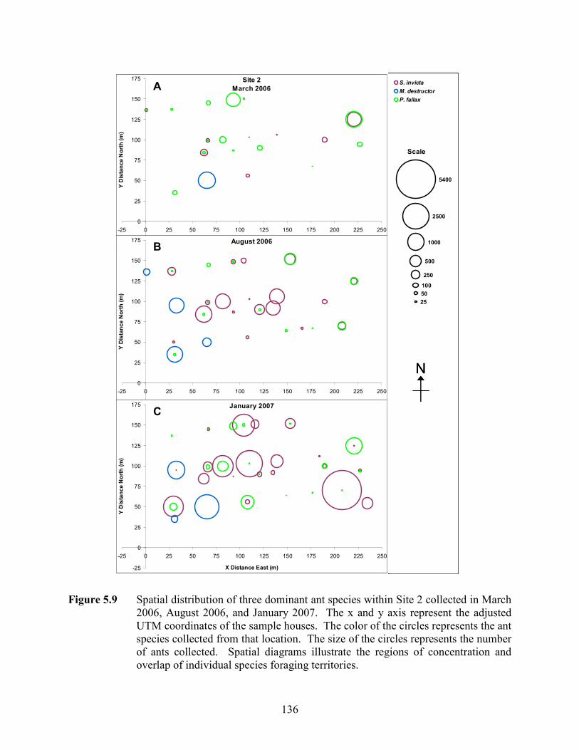
136

N

Scale

25

50

100

250

500

1000

2500

5400

S. invicta

M. destructor

P. fallax

Site 2

March 2006

-25

0

25

50

75

100

125

150

175

-25 0 25 50 75 100 125 150 175 200 225 250


August 2006

-25

0

25

50

75

100

125

150

175

-25 0 25 50 75 100 125 150 175 200 225 250


January 2007

-25

0

25

50

75

100

125

150

175

-25 0 25 50 75 100 125 150 175 200 225 250

X Distance East (m)


A

C

B

N

Scale

25

50

100

250

500

1000

2500

5400

S. invicta

M. destructor

P. fallax

Site 2

March 2006

-25

0

25

50

75

100

125

150

175

-25 0 25 50 75 100 125 150 175 200 225 250


August 2006

-25

0

25

50

75

100

125

150

175

-25 0 25 50 75 100 125 150 175 200 225 250


January 2007

-25

0

25

50

75

100

125

150

175

-25 0 25 50 75 100 125 150 175 200 225 250

X Distance East (m)


NN

Scale

25

50

100

250

500

1000

2500

5400

S. invicta

M. destructor

P. fallax

Site 2

March 2006

-25

0

25

50

75

100

125

150

175

-25 0 25 50 75 100 125 150 175 200 225 250


August 2006

-25

0

25

50

75

100

125

150

175

-25 0 25 50 75 100 125 150 175 200 225 250


January 2007

-25

0

25

50

75

100

125

150

175

-25 0 25 50 75 100 125 150 175 200 225 250

X Distance East (m)


A

C

B

Figure 5.9 Spatial distribution of three dominant ant species within Site 2 collected in March

2006, August 2006, and January 2007. The x and y axis represent the adjusted UTM coordinates of the sample houses. The color of the circles represents the ant species collected from that location. The size of the circles represents the number of ants collected. Spatial diagrams illustrate the regions of concentration and overlap of individual species foraging territories.

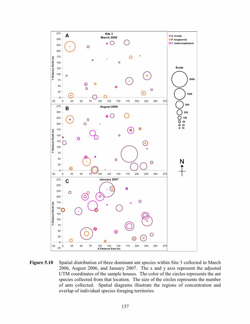
137

N

Scale

10

25

50

100

250

500

1000

2000

S. invicta

P. longicornis

T. melanocephalum

Site 3

March 2006

-25

0

25

50

75

100

125

150

175

200

225

250

275

-25 0 25 50 75 100 125 150 175 200 225 250 275


August 2006

-25

0

25

50

75

100

125

150

175

200

225

250

275

-25 0 25 50 75 100 125 150 175 200 225 250 275


January 2007

-25

0

25

50

75

100

125

150

175

200

225

250

275

-25 0 25 50 75 100 125 150 175 200 225 250 275X Distance East (m)


A

C

B

N

Scale

1025

50

100

250

500

1000

2000

S. invicta

P. longicornis

T. melanocephalum

Site 3

March 2006

-25

0

25

50

75

100

125

150

175

200

225

250

275

-25 0 25 50 75 100 125 150 175 200 225 250 275


August 2006

-25

0

25

50

75

100

125

150

175

200

225

250

275

-25 0 25 50 75 100 125 150 175 200 225 250 275


January 2007

-25

0

25

50

75

100

125

150

175

200

225

250

275

-25 0 25 50 75 100 125 150 175 200 225 250 275X Distance East (m)


NN

Scale

1025

50

100

250

500

1000

2000

S. invicta

P. longicornis

T. melanocephalum

Site 3

March 2006

-25

0

25

50

75

100

125

150

175

200

225

250

275

-25 0 25 50 75 100 125 150 175 200 225 250 275


August 2006

-25

0

25

50

75

100

125

150

175

200

225

250

275

-25 0 25 50 75 100 125 150 175 200 225 250 275


January 2007

-25

0

25

50

75

100

125

150

175

200

225

250

275

-25 0 25 50 75 100 125 150 175 200 225 250 275X Distance East (m)


A

C

B

Figure 5.10 Spatial distribution of three dominant ant species within Site 3 collected in March 2006, August 2006, and January 2007. The x and y axis represent the adjusted UTM coordinates of the sample houses. The color of the circles represents the ant species collected from that location. The size of the circles represents the number of ants collected. Spatial diagrams illustrate the regions of concentration and overlap of individual species foraging territories.

138

CHAPTER 6. SUMMARY

The Swiss botanist Alphonse De Candolle (1806-1893) once described the succession of

plants by saying, “All the plants of a given country…are at war with one another. The first

which establish themselves by chance in a particular spot, tend, by the mere occupancy of space,

to exclude other species – the greater choke the smaller, the longest livers replace those who last

for a shorter period, the more prolific gradually make themselves masters of the ground, which

species multiplying more slowly would otherwise fill” (Irvine 1955). In fact, during succession

many different organisms within an environment are “at war with one another.” While the

succession of plants has been well documented, the succession of another group of organisms,

ants, has also been studied (Majer 1984, Haering and Fox 1987, MacKay 1993). Candolle could

have just as easily replaced “plants” with “ants” and his quote would still have been an accurate

description of succession.

There have been numerous studies documenting the succession of ants in recovering

habitats. However, these studies have been almost exclusively conducted in disturbed natural

environments. Few studies have examined the succession of pest ants in disturbed urban

environments. In general, little is known about the ecology of pest ant species in urban habitats,

specifically in the tropics (Fowler and Bueno 1996). However, the island of Puerto Rico

provided an ideal setting in which to study the succession of pest ant species in urban

environments. The land use patterns in Puerto Rico, as they have changed from forest to

agriculture to urban sprawl, have resulted in a mosaic of housing developments of different ages

(Grau et al. 2003). These developments represent different stages of urban succession. These

housing developments have been subsequently overrun with many different ant species

representing increases in species biodiversity. Although the ants of Puerto Rico have been well

studied (Wheeler 1908, Smith 1936, Levins et al. 1973, and Torres and Snelling 1997), the urban

pest ant complex has not been specifically identified or quantified in terms of biodiversity.

Therefore, three housing developments in Santa Isabel, Puerto Rico each representing different

periods in the successional process were chosen to study the pest ant species complex in regard

to species biodiversity and spatial partitioning of foraging ranges.

139

The youngest housing development was one year old (Site 1) and represented an

environment in the early stages of succession after a disturbance (construction). A total of 14

species and over 58,000 ants were collected from Site 1 over the course of the study. Of these 14

species, six represented the founding species complex (S. invicta, S. globularia, Brachymyrmex

sp. 1, P. moerens, P. fallax, and P. longicornis). Three species in particular (S. invicta,

Brachymyrmex sp. 1, and P. moerens) were dominant throughout the site and represented the

greatest ant biomass at the earliest stage of succession.

As expected, biodiversity measures of richness, abundance, and diversity were all

significantly lower for Site 1 than the two older sites. Richness and abundance measures were

determined based on the number of species and ants, respectively, collected at each sample house

during a sampling period. A mean of 2.2 species and 244 ants were collected from every sample

house over eight sampling periods (March 2006 – January 2007). Diversity indices were

calculated based on the number of species and relative abundance of each species collected from

each sample house. The mean diversity index for the houses in Site 1 was 0.38. Bormann and

Likens’ (1981) model of biomass accumulation indicated that the least amount of biomass would

be present at the beginning of the aggradation stage of succession, which is shortly after a

disturbance has occurred. Because both the abundance and diversity was the least in Site 1, our

data suggested that Site 1 was in the early stage of succession described by Bormann and Likens

(1981).

Although Site 1 was in the earliest stages of succession, our spatial diagrams indicated

that many species were already established. In fact, multiple species were collected from the

same sample houses, which indicated that the species at those houses had overlapping foraging

ranges. Over the course of the test period, the founding species and later arriving species

continued to increase their abundance and spread to more sample houses in Site 1. Coexistence

was even observed between the dominant species (S. invicta, Brachymyrmex sp. 1, and P.

moerens). S. invicta and Brachymyrmex sp. 1 were already well established throughout Site 1 at

the beginning of the test in March 2006. However, P. moerens was only present in the

southeastern corner of the site. Yet by the end of the test period, P. moerens had also spread

throughout Site 1. The range expansion of P. moerens indicated that this species was in the

process of becoming established at Site 1 during the test period. Although Site 1 had some

spatial partitioning between the three dominant species at the beginning of the year, as the

140

abundances of all three species increased over the test period, spatial partitioning was reduced

and coexistence increased.

At four years of age, Site 2 represented a mid-successional housing development. This

housing development was near the peak of the aggradation stage of succession. The greatest

number of ants was collected from Site 2 (> 99,000 ants over the course of one year) and the

second greatest number of species (20). S. invicta, M. destructor, and P. fallax represented the

dominant mid-successional species in Site 2.

Biodiversity measures of richness, abundance, and diversity were significantly greater in

Site 2 than in the one-year-old site, which indicated that Site 2 was at a later stage of succession.

A mean of 3.1 species and 407 ants were collected from every sample house in Site 2 over the

course of the test. The mean diversity index for a sample house in Site 2 was 0.51. Because Site

2 had the greatest abundance of ants, the peak biomass corresponded with the end of the

aggradation stage and the beginning of the transition stage described in Bormann and Liken’s

(1981) model of succession. Although Site 2 had the greatest ant biomass, the diversity index of

Site 2 was still significantly lower than of the oldest site (Site 3).

Over the course of the test period, increases in the abundance and coexistence of the mid-

successional species were observed in Site 2. Sampled ant abundance tripled from 8,000 in

March 2006 to > 24,000 ants by January 2007. The spatial diagrams indicated that multiple

species inhabited the same houses by January 2007 (3.5 species). The dominant species, S.

invicta and P. fallax, also expanded their range and abundance throughout the site over the test

period. Interestingly, the other dominant species, M. destructor, did not expand its range or

abundance over the year and was only collected at a few locations in large concentrations.

Although M. destructor did not spread throughout the site, their large numbers appeared to

exclude the establishment of the other species. Even the other two dominant species (S. invicta

and P. fallax) did not forage in locations where M. destructor was established. S. invicta and P.

fallax were however often found coexisting together at the same houses which indicated little or

no spatial partitioning between these two dominant species.

The oldest housing development was eight years old (Site 3). Site 3 represented the most

advanced stage of succession of the three housing developments. The greatest number of species

(21 species) and the second greatest number of individual ants (> 88,000) were collected from

Site 3. The dominant species complex consisted of five species. S. invicta was the most

141

abundant species (46% relative abundance). The other dominant species included P. fallax, P.

longicornis, P. moerens, and T. melanocephalum, with relative abundances ranging from 7-14%.

Site 3 had the greatest diversity and evenness indices of the three sites (0.61 and 0.13,

respectively). These two indices were the main indication that Site 3 was in a more advanced

stage of succession than either Site 1 or Site 2 (Molles 2005). Although Site 3 had a greater

diversity index, less ant biomass was collected in Site 3 than in Site 2. According to the biomass

accumulation model (Bormann and Likens 1981), a decrease in biomass occurs during the

transition stage. Therefore, we concluded that Site 3 was in the transition stage, after the peak in

biomass had occurred. However, the richness and abundance value calculated for Site 2 and 3

were not significantly different. This lack of difference between Site 2 and 3 suggested that Site

3 was still in the transition stage of succession and had not yet reached a steady state or a climax

community.

Sample houses in Site 3 had a greater number of species coexisting than in Site 2. The

most dominant species, S. invicta, was found to coexist with either P. longicornis or T.

melanocephalum throughout Site 3. However, P. longicornis and T. melanocephalum were

rarely collected from the same house indicating spatial partitioning between these two species.

The peak population in T. melanocephalum abundance (January 2007) corresponded with a

decline in P. longicornis which may have suggested that these two species were competing for

similar resources, but that T. melanocephalum was more successful.

The results of this study indicated that each housing development had a diverse complex

of ant species. Not surprisingly, many of the dominant species in each site were invasive or

tramp species which were adapted to invade and survive in disturbed urban environments.

Although there were different ant complexes in each site, similar trends of individual species

increasing their frequency and abundance over time, were observed in all sites. These increases

in abundance and frequency appeared in several cases to be related to seasonal rainfall. The

increases in abundance also resulted in many overlapping foraging ranges, with many species

coexisting at the same location. In other words, spatial partitioning was not common.

Majer (1983) proposed, “ant communities change as succession proceeds,” and our

research findings supported this statement. Based on the differences in the biodiversity

measures, each site represented a different period in the successional process with a different ant

community. As the age of the site increased, so too did the diversity of the site. Ant abundance

142

totals from each site appeared to follow the biomass accumulation model for succession. Site 1

represented early succession near the beginning of the aggradation stage. Six species collected

from Site 1 in March 2006 represented the founding species complex of these disturbed urban

environments. Site 2 had the greatest biomass, and the ant species collected in Site 2 represented

a mid-successional complex associated with the transition stage of succession. Site 3 had the

greatest ant species diversity and evenness. Site 3 represented a stage of succession approaching

steady state and the beginning of a climax community. Yet, the similarity of Site 3 to Site 2

suggests that Site 3 had not yet reached the steady state. We believe that further research in

older housing developments (> 15 years old) would reveal a tramp ant species complex that was

characteristic of the steady state of urban succession. Therefore, additional research is necessary

in order to identify the climax ant communities present in the disturbed urban environments of

Puerto Rico.

143

LITERATURE CITED

Adams, E. S. 1994. Territory defense by the ant Azteca trigona: maintenance of an arboreal ant

mosaic. Oecologia. 97: 202-208. Adams, C. T., J. K. Plumley, W. A. Banks, and C. S. Lofgren. 1977. Impact of red imported fire

ant, Solenopsis invicta Buren (Hymenoptera: Formicidae) on harvest of soybean in North Carolina. J. Elisha Mitch. Sci. Soc. 93: 150-152.

Adams, C. T., W. A. Banks, C. S. Lofgren, B. J. Smittle, and D. P. Harlan. 1983. Impact of the

red imported fire ant, Solenopsis invicta (Hymenoptera: Formicidae), on the growth and yield of soybeans. J. Econ. Entomol. 76: 1129-1132.

Agosti, D., J. D. Majer, L. E. Alonso, and T. R. Schultz. 2000. Ants: standard methods for

measuring and monitoring biodiversity. Smithsonian Institution Press, Washington D.C. Aide, T. M., J. K. Zimmerman, J. B. Pascarella, L. Rivera, and H. Marcano-Vega. 2000. Forest

regeneration in a chronosequence of tropical abandoned pastures: implications for restoration ecology. Restor. Ecol. 8: 328-338.

Allendorf, F. W., and L. L. Lundquist. 2003. Introduction: population biology, evolution, and

control of invasive species. Conserv. Biol. 17: 24-30. Andersen, A. N. 1992. Regulation of “momentary” diversity by dominant species in

exceptionally rich ant communities of the Australian seasonal tropics. Am. Nat. 140: 401-420.

Ayre, G. L. 1977. Exotic ants in Winnipeg, Manitoba. Entomologist. 11: 4111-4144. Banks, W. A., and D. F. Williams. 1989. Competitive displacement of Paratrechina longicornis

(Latreille) (Hymeoptera: Formicidae) from baits by fire ants in Mato Grosso, Brazil. J. Entomol. Sci. 24: 381-391.

Bastl, M., P. Kocar, K. Parch, and P. Pysek. 1997. The effect of successional age and disturbance

on the establishment of alien plants in man-made sites: an experimental approach, pp. 191-201. In J. H. Brock, M. Wade, P. Pysek, and D. Green [eds.], Plant invasions: studies from North America and Europe. Backhuys Publishers, Leiden, Netherlands.

Berry, J. A., O. R. Green, and S. O. Shattuck. 1997. Species of Pheidole Westwood

(Hymenoptera: Formicidae) established in New Zealand. N. Z. J. Zool. 24: 25-33. Bolton, B. 1987. A review of the Solenopsis genus-group and revision of Afrotropical

Monomorium Mayr (Hymenoptera: Formicidae). Bull. Br. Mus. Entomol. Ser. 54: 263-452.

144

Bolton, B. 1994. Identification guide to the ant genera of the world. Harvard University Press, Cambridge, MA.

Bolton, B. 1995. A new general catalogue of the ants of the world. Harvard University Press,

Cambridge, MA. Bormann, F. H. and Likens, G. E. 1981. Pattern and process in a forested ecosystem. Springer-

Verlag, New York. Bradshaw, A. D. 1993. Introduction: understanding the fundamentals of succession, pp. 1-3. In J.

Miles and D. W. H. Walton [eds.], Primary succession on land. Blackwell Scientific Publications, Oxford, UK.

Briese, D. T., and B. J. Macauley. 1977. Physical structure of an ant community in semi-arid

Australia. Aust. J. Ecol. 2: 107-120. Carroll, C. R., and D. H. Janzen. 1973. Ecology of foraging by ants. Annu. Rev. Ecol. Syst. 4:

231-257. Chapin, F. S., L. R. Walker, C. L. Fastie, and L. C. Sharman. 1994. Mechanisms of primary

succession following deglaciation at Glacier Bay, Alaska. Ecol. Monogr. 64: 149-175. Cherry, R. H., and G. S. Nuessly. 1992. Distribution and abundance of imported fire ants

(Hymenoptera: Formicidae) in Florida sugarcane fields. Environ. Entomol. 21: 767-770. Chinea, J. D., and E. H. Helmer. 2003. Diversity and composition of tropical secondary forests

recovering from large-scale clearing: results from the 1990 inventory in Puerto Rico. For. Ecol. Manage. 180: 227-240.

Claborn, D. M., and S. A. Phillips, Jr. 1986. Temporal foraging activities of Solenopsis invicta

(Hymenoptera: Formicidae) and other predominant ants of central Texas. Southwest. Nat. 31: 555-557.

Clark, D. B., C. Guayasamin, O. Pazmino, C. Donoso, and Y. Paez de Villacis. 1982. The tramp

ant Wasmannia auropunctata: autecology and effects on ant diversity and distribution on Santa Cruz Island, Galapagos. Biotropica. 14: 196-201.

Clements, F. E. 1916. Plant succession: an analysis of the development of vegetation. Carnegie

Institution of Washington, Washington, D.C. Cohen, P. R. 1992. Imported fire ant stings: clinical manifestations and treatment. Pediatr.

Dermatol. 9: 44-48. Colautti, R. I., and H. J. MacIsaac. 2004. A neutral terminology to define ‘invasive’ species.

Divers. Distrib. 10: 135-141.

145

Cole, F. R., A. C. Medeiros, L. L. Loope, and W. W. Zuehlke. 1992. Effects of the Argentine ant on arthropod fauna of Hawaiian high-elevation shrubland. Ecology. 73: 1313-1322.

Collingwood, C. A., B. J. Tigar, and D. Agosti. 1997. Introduced ants in the United Arab

Emirates. J. Arid Environ. 37: 505-512. Collins, L., and R. H. Scheffrahn. 2008. Featured creatures: Solenopsis invicta (Buren), red

imported fire ant. University of Florida, Institute of Food and Agricultural Sciences, Gainesville, FL. (http://www.entnemdept.ufl.edu/creatures/urban/ants/red_imported_fire_ant.htm).

Connell, J. H., and R. O. Slatyer. 1977. Mechanisms of succession in natural communities and

their role in community stability and organization. Am. Nat. 111: 1119-1144. Cook, J. L. 2003. Conservation of biodiversity in an area impacted by the red imported fire ant,

Solenopsis invicta (Hymenoptera: Formicidae). Biodivers. Conserv. 12: 187-195. Cowles, H. C. 1911. The causes of vegetative cycles. Bot. Gaz. 51: 161-183. Creighton, W. S. 1950. The ants of North America. Bull. Mus. Comp. Zool. 104: 1-585. Creighton, W. S., and R. R. Snelling. 1974. Notes on the behavior of three species of

Cardiocondyla in the United States (Hymenoptera: Formicidae). J. N.Y. Entomol. Soc. 82: 82–92.

Crouch, H. J. 1993. Plant distribution patterns and primary succession on a glacier foreland: a

comparative study of cryptogams and higher plants, pp. 133-145. In J. Miles and D. W. H. Walton [eds.], Primary succession on land. Blackwell Scientific Publications, Oxford, UK.

Culver, D. C. 1974. Species packing in Caribbean and north temperate ant communities.

Ecology. 4: 974-988. Daane, K. M., K. R. Sime, J. Fallon, and M. L. Cooper. 2007. Impacts of Argentine ants on

mealybugs and their natural enemies in California’s coastal vineyards. Ecol. Entomol. 32: 583-596.

Davis, P. R., J. J. Van Schagen, M. A. Widmer, and T. J. Craven. 1993. A review of Argentine

ant research in Western Australia. Agricultural Protection Board of Western Australia, Perth, Western Australia. 95 pp.

De Wet, A. P., J. Richardson, and C. Olympia. 1998. Interactions of land-use history and current

ecology in a recovering “urban wildland.” Urban Ecosyst. 2: 237-262. Del Moral, R. 1993. Mechanisms of primary succession on volcanoes: a view from Mount St.

Helens, pp. 79-100. In J. Miles and D. W. H. Walton [eds.], Primary succession on land. Blackwell Scientific Publications, Oxford, UK.

146

Deyrup, M. A. 1991. Exotic ants of the Florida Keys, pp. 15-22. In W. H. Eshbaugh [ed.],

Proceedings of the 4th Symposium on the Natural History of the Bahamas. Bahamian Field Station, San Salvador, Bahamas.

Deyrup, M., L. Davis, and S. Cover. 2000. Exotic ants in Florida. T. Am. Entomol. Soc. 126:

293-326. Diaz, R., A. Knutson, and J. S. Bernal. 2004. Effect of the red imported fire ant on cotton aphid

population density and predation of bollworm and beet armyworm eggs. J. Econ. Entomol. 97: 222-229.

Dietz, J. L. 1989. Historica economica de Puerto Rico. Ediciones Huracan Inc., Rio Piedras,

Puerto Rico. Diffie, S., and C. Sheppard. 1990. Impact of imported fire ants on Georgia homeowners, pp. 62-

71. In M. E. Mispagel [ed.], 1990 Imported Fire Ant Conference. Texas A&M University, College Station, Texas.

Don, W., and R. Harris. 2005. Ant information sheet number 22: Pheidole megacephala. Series

of unpublished Landcare Research contract reports to Biosecurity New Zealand. Landcare Research, Lincoln, New Zealand.

Dureau de la Malle, A. J. C. A. 1825. Memoire sur l'alternance ou sur ce probleme: la succession

alternative dans la reproduction des especes vegetales vivant en societe, est-elle une loi generale de la nature? Ann. Sci. Nat. 1. 5: 353-381.

Ebdon, D. 1985. Statistics in geography, 2nd ed. Basil Blackwell Ltd., New York, NY. Elliott, J. M. 1971. Some methods for the statistical analysis of samples of benthic invertebrates.

Sci. Publ. 25. Freshwater Biol. Ass., Ambleside, Westmorland, U.K. Ferster, B., M. Deyrup, and R. H. Scheffrahn. 2000. The pest ants of Florida. Fort Lauderdale

R.E.C. Research Report FTL 00-1, Fort Lauderdale, FL. 22 pp. Ferster, B., M. Deyrup, R. H. Scheffrahn, and B. J. Cabrera. 2002. The pest ants of Florida.

University of Florida, Fort Lauderdale Research and Education Center, Fort Lauderdale, FL. (http://flrec.ifas.ufl.edu/entomo/ants/Pest%20Ants%20of%20FL/).

Figueroa Colon, J. C. 1996. The scientific survey of Puerto Rico and the Virgin Islands: an

eighty-year reassessment of the islands' natural history. Ann. N. Y. Acad. Sci. 776: 1-273. Fowler, H. G., and O. C. Bueno. 1996. Congruent spatial and temporal foraging by a dominant

ant (Hym., Formicidae) and its replacement in an assemblage in a large urban structure in southeastern Brazil. J. Appl. Entomol. 120: 29-32.

147

Fowler, H. G., L. E. Alves, and O. C. Bueno. 1993. Reproductive strategies of the exotic Pharaoh’s ant Monomorium pharaonis (L.) (Hymenoptera: Formicidae) in Brazil. Invertebr. Reprod. Dev. 23: 235-238.

Franco, P. A., P. L. Weaver, and S. Eggen-McIntosh. 1997. Forest resources of Puerto Rico,

1990. U.S. Department of Agriculture, Forest Service, Southern Research Station, Asheville, N.C.

Gaston, K. J. 1996. What is biodiversity?, pp. 1-9. In K. J. Gaston [ed.], Biodiversity: a biology

of numbers and difference. Blackwell Science Ltd., Oxford, U.K. [GISD] Global Invasive Species Database. 2006a. Monomorium destructor. National Biological

Information Infrastructure and IUCN/SSC Invasive Species Specialist Group. (http://www.invasivespecies.net/database/species/ecology.asp?si=960&fr=1&sts=sss&lang=EN).

[GISD] Global Invasive Species Database. 2006b. Pheidole megacephala. IUCN/SSC Invasive

Species Specialist Group. (http://www.invasivespecies.net/database/species/ecology.asp?si=132&fr=1&sts=sss&lang=EN).

[GISD] Global Invasive Species Database. 2006c. Solenopsis invicta. IUCN/SSC Invasive

Species Specialist Group. (http://www.invasivespecies.net/database/species/ecology.asp?si=77&fr=1&sts=sss&lang=EN).

Goddard, J. 1996. Physicians guide to arthropods of medical importance. CRC Press, New York,

NY. Golley, F. B. 1977. Ecological succession: benchmark papers in ecology, No. 5. Dowden,

Hutchinson and Ross, Inc., Stroudsburg, PA. Gomez, C., P. Pons, and J. M. Bas. 2003. Effects of the Argentine ant Linepithema humile on

seed dispersal and seedling emergence of Rhamnus alaternus. Ecography. 26: 532-538. Graham, J. H., H. H. Hughie, S. Jones, K. Wrinn, A. J. Krzysik, J. J. Duda, D. C. Freeman, J. M.

Emlen, J. C. Zak, D. A. Kovacic, C. Chamberlin-Graham, and H. Balbach. 2004. Habitat disturbance and the diversity and abundance of ants (Formicidae) in the Southeastern Fall-Line Sandhills. J. Insect Sci. 4: 30.

Grau, H. R., T. M. Aide, J. K. Zimmerman, J. R. Thomlinson, E. Helmer, and X. Zou. 2003. The

ecological consequences of socioeconomic and land-use changes in postagriculture Puerto Rico. Bioscience. 53: 1159-1168.

Grundmann, A. W. 1952. The new Brachymyrmex from northern Utah (Hymenoptera:

Formicidae). J. Kans. Entomol. Soc. 25: 117.

148

Haering, R., and B. J. Fox. 1987. Short-term coexistence and long-term competitive

displacement of two dominant species of Iridomyrmex: the successional response of ants to regenerating habitats. J. Anim. Ecol. 56: 495-507.

Harada, A. Y. 1990. Ant pests of the Tapinomini tribe, pp. 298-315. In R. K. Vander Meer, K.

Jaffe, and A. Cedeno [eds.], Applied myrmecology: a world perspective. Westview Press, Boulder, CO.

Harris, R. 2005a. Invasive ant risk assessment: Monomorium destructor. Series of unpublished

Landcare Research contract reports to Biosecurity New Zealand. Landcare Research, Lincoln, New Zealand.

Harris, R. 2005b. Invasive ant risk assessment: Tapinoma melanocephalum. Series of

unpublished Landcare Research contract reports to Biosecurity New Zealand. Landcare Research, Lincoln, New Zealand.

Harris, R., and K. Abbott. 2005. Invasive ant risk assessment: Paratrechina longicornis. Series

of unpublished Landcare Research contract reports to Biosecurity New Zealand. Landcare Research, Lincoln, New Zealand.

Hedges, S. A. 1992. Field guide for the management of structure-infesting ants. Franzak and

Foster Co., Cleveland, OH. Hedges, S. A. 1997. Chapter 12: Ants, pp. 503-589. In A. Mallis and D. Moreland [eds.]

Handbook of pest control: the behavior, life history, and control of household pests, 8th ed. Mallis Handbook and Technical Training Company.

Hedges, S. A. 1998. Field guide for the management of structure-infesting ants, 2nd ed. GIE

Publishing, Cleveland, OH. Hedlund, K. S. 2006. Genus Brachymyrmex. University of North Carolina, Chapel Hill, NC.

(http://www.cs.unc.edu/~hedlund/playpen/ants/GenusPages/Formicinae/ Brachymyrmex.html).

Heinze, J. J. 1999. Male polymorphism in the ant species Cardiocondyla minutior

(Hymenoptera: Formicidae). Entomol. Gen. 23: 251-258. Heinze, J. J., S. Kuhnholz, K. Schilder, and B. Hölldobler. 1993. Behaviour of ergatoid males in

the ant, Cardiocondyla nuda. Insect. Soc. 40: 273-282. Helmer, E. H. 2004. Forest conservation and land development in Puerto Rico. Landscape Ecol.

19: 29-40.

149

Helmer, E. H., O. Ramos, T. del M. Lopez, M. Quinones, and W. Diaz. 2002. Mapping the forest type and land cover of Puerto Rico, a component of the Caribbean biodiversity hotspot. Caribb. J. Sci. 38: 165-183.

Henneberry, T. J., L. Forlow Jech, T. de la Torre, and D. L. Hendrix. 2000. Cotton aphid

(Homoptera: Aphididae): biology, honeydew production, sugar quality and quantity, and relationships to sticky cotton. Southwest. Entomol. 25: 161-174.

Holldobler, B., and E. O. Wilson. 1990. The ants. Harvard University Press, Cambridge, MA. Holway, D. A., L. Lach, A. V. Suarez, N. D. Tsutsui, and T. J. Case. 2002. The causes and

consequences of ant invasions. Ann. Rev. Ecol. Syst. 33: 181-233. Horton, J. R. 1918. The Argentine ant in relation to citrus groves. Bulletin 647. U.S. Department

of Agriculture, Washington, D.C.

Irvine, W. 1955. Apes, angels, and Victorians; the story of Darwin, Huxley, and evolution. McGraw-Hill, New York, NY.

Jackson, D. A. 1984. Ant distribution patterns in a Cameroonian cocoa plantation: investigation

of the ant mosaic hypothesis. Oecologia. 62: 318-324. Jaffe, K. 1993. Surfing ants. Fla. Entomol. 76: 182-183. Johnston, D. W., and E. P. Odum. 1956. Breeding bird populations in relation to plant succession

on the piedmont of Georgia. Ecology. 37: 50-62. Jonas, J. L., M. R. Whiles, and R. E. Charlton. 2002. Aboveground invertebrate responses to land

management differences in a central Kansas grassland. Environ. Entomol. 31: 1142-1152. Kaplan, I., and M. Eubanks. 2002. Disruption of cotton aphid (Homoptera: Aphididae)-natural

enemy dynamics by red imported fire ants (Hymenoptera: Formicidae). Environ. Entomol. 31: 1175-1183.

Klotz, J. 2004. Chapter 11: Ants, pp. 635-693. In A. Mallis and D. Moreland [eds.] Handbook of

pest control: the behavior, life history, and control of household pests, 9th ed. GIE Media, Cleveland, OH.

Klotz, J. H., J. R. Mangold, K. M. Vail, L. R. Davis Jr., and R. S. Patterson. 1995. A survey of

the urban pest ants (Hymenoptera: Formicidae) of peninsular Florida. Fla. Entomol. 1: 109-118.

Korzukhin, M. D., S. D. Porter, L. C. Thompson, and S. Wiley. 2001. Modeling temperature-

dependent range limits for the fire ant Solenopsis invicta (Hymenoptera: Formicidae) in the United States. Environ. Entomol. 30: 645-655.

150

Krebs, C. J. 1998. Ecological Methodology, 2nd ed. Benjamin Cummings, Menlo Park, CA. Laakkonen, J., R. N. Fisher, T. J. Case. 2001. Effect of land cover, habitat fragmentation and ant

colonies on the distribution and abundance of shrews in southern California. J. Anim. Ecol. 70: 776-788.

Lach, L. 2003. Invasive ants: unwanted partners in ant-plant interactions? Ann. Mo. Bot. Gard.

90: 91-108. Lavigne, R. J. 1977. Notes on the ants of Luquillo Forest, Puerto Rico (Hymenoptera:

Formicidae). Proc. Entomol. Soc. Wash. 2: 216-237. Lee, C.Y. 2002. Tropical household ants: pest status, species diversity, foraging behavior, and

baiting studies, pp. 3-18. In S. C. Jones, J. Zhai, and W. H. Robinson [eds.], Proceedings of the 4th international conference on urban pests. Pocahontas Press Inc., Blacksburg, VA.

Lee, C.Y., and Robinson, W.H. 2001. Handbook of Malaysian Household and Structural Pests.

Pest Control Association of Malaysia, Kuala Lumpur, Malaysia. Lennartz, F. E. 1973. Modes of dispersal of Solenopsis invicta from Brazil into the continental

United States – a study in spatial diffusion. M.S. thesis, University of Florida, Gainesville, FL.

Levings, S. C. 1983. Seasonal, annual, and among-site variation in the ground ant community of

a deciduous tropical forest: some causes of patchy species distributions. Ecol. Monogr. 53: 435-455.

Levings, S. C., and J. F. A. Traniello. 1981. Territoriality, nest dispersion, and community

structure in ants. Psyche. 88: 265-320. Levins, R., M. L. Pressick, and H. Heatwole. 1973. Coexistence patterns in insular ants. Am. Sci.

4: 463-472. Lim, D., and J. Pickering. 2008. Formicidae. Discover Life, University of Georgia, Athens, GA.

(http://www.discoverlife.org/20/q?search=Formicidae). Lindenmayer, D. B., C. R. Margules, and D. B. Botkin. 2000. Indicators of biodiversity for

ecologically sustainable forest management. Conserv. Biol. 14: 941-950. Lofgren, C. S. 1986. The economic importance and control of imported fire ants in the United

States, pp 227-256. In S. B. Vinson [ed.], Economic impact and control of social insects. Praeger Publishers, New York, NY.

Lofgren, C. S., W. A. Banks, and B. M. Glancey. 1975. Biology and control of imported fire

ants. Annu. Rev. Entomol. 20:1-30.

151

Longino, J. T. 2004. Brachymyrmex Overview. The Evergreen State College, Olympia, WA. (http://academic.evergreen.edu/projects/ants/genera/brachymyrmex/home.html).

Longino, J. T., and S. Cover. 1997. Pheidole fallax Mayr 1870. University of Georgia, Athens,

GA. (http://www.discoverlife.org/mp/20q?search=Pheidole+fallax). López, T. del M., T. M. Aide, and J. R. Thomlinson. 2001. Urban expansion and the loss of

prime agricultural lands in Puerto Rico. Ambio. 30: 49-54. MacArthur, R. H., and J. W. MacArthur. 1961. On bird species diversity. Ecology. 42: 594-598. MacGown, J. A., J. G. Hill, and M. A. Deyrup. 2007. Brachymyrmex patagonicus

(Hymenoptera: Formicinae), an emerging pest species in the southeastern United States. Fla. Entomol. 90: 457-464.

MacKay, W. P. 1993. Succession of ant species (Hymenoptera: Formicidae) on low-level nuclear

waste sites in northern New Mexico. Sociobiology. 23: 1-11. Magurran, A. E. 1988. Ecological diversity and its measurement. Princeton University Press,

Princeton, NJ. Majer, J. D. 1981. The role of invertebrates in minesite rehabilitation. Forests Department of

Western Australia Bulletin. 93: 29. Majer, J. D. 1983. Ants – useful bio-indicators of minesite rehabilitation, land-use and land

conservation. Environ. Manage. 7: 375-383. Majer, J. D. 1984. Recolonization by ants in rehabilitated open-cut mines in Northern Australia.

Reclam. Reveg. Res. 2: 279-298. Majer, J. D., and K. R. Brown. 1986. The effects of urbanization on the ant fauna of the Swan

Coastal Plain near Perth, Western Australia. J. R. Soc. West. Aust. 69: 13-17. Majer, J. D., M. Sartori, R. Stone, and W. S. Perriman. 1982. Colonization by ants and other

invertebrates in rehabilitated mineral sand mines near Eneabba, Western Australia. Reclam. Reveg. Res. 1: 63-81.

Mandryk, A. M., and R. W. Wein. 2006. Exotic vascular plant invasiveness and forest

invasibility in urban boreal forest types. Biol. Invasions. 8: 1651-1662. Mann, C. C. 1994. Fire ants parlay their queens into a threat to biodiversity. Science. 263: 60-61. Markin, G. P., J. H. Dillier, and H. L. Collins. 1973. Growth and development of colonies of the

red imported fire ant, Solenopsis invicta. Ann. Entomol. Soc. Am. 66: 803-808.

152

Marrs, R. H., and A. D. Bradshaw. 1993. Primary succession on man-made wastes: the importance of resource acquisition, pp. 221-248. In J. Miles and D. W. H. Walton [eds.], Primary succession on land. Blackwell Scientific Publications, Oxford, UK.

McGlynn, T. P. 1999. The worldwide transfer of ants: geographical distribution and ecological

invasions. J. Biogeogr. 26: 535-548. McIntyre, N. E. 2000. Ecology of urban arthropods: a review and a call to action. Ann. Entomol.

Soc. Am. 93: 825-835. Miles, J., and D. W. H. Walton. 1993. Primary succession on land. Blackwell Scientific

Publications, Oxford, UK. Mitich, L. W. 1992. Succession in urban areas, pp. 47-50. In Proceedings, California Weed

Conference, 20-22 January, 1992, Sacramento, California. Mobley, D., and J. Redding. 2005. USDA amends imported fire ant quarantine. USDA-APHIS

Press Releases. (http://www.aphis.usda.gov/lpa/news/2005/08/fireantq_ppq.html).

Molles, M. C. J. 2005. Ecology: concepts and applications, 3rd ed. McGraw-Hill, New York, NY. Morris, W. F., and D. M. Wood. 1989. The role of lupine in succession on Mount St. Helens:

facilitation or inhibition? Ecology. 70: 697-703. Morrison, L. W., S. D. Porter, E. Daniels, and M. D. Korzukhin. 2004. Potential global range

expansion of the invasive fire ant, Solenopsis invicta. Biol. Invasions. 6: 183-191. Nagle, G. 1999. Britain’s Changing Environment. Nelson Thornes, Surrey, UK. Nansen, C., J. F., Campbell, T. W. Phillips, and M.A. Mullen. 2003. The impact of spatial

structure on the accuracy of contour maps of small data sets. J. Econ. Entomol. 96: 1617-1625.

[NCSS] National Cooperative Soil Survey. 2007. Santa Isabel Series.

(http://www2.ftw.nrcs.usda.gov/osd/dat/S/SANTA_ISABEL.html). [NOAA] National Oceanic and Atmospheric Administration. 2006. National Weather Service

Forecast Office: San Juan, PR. (http://www.weather.gov/climate/local_data.php?wfo=sju).

Ness, J. H., and J. L. Bronstein. 2004. The effects of invasive ants on prospective ant mutualists.

Biol. Invasions. 6: 445-461.

153

Nickerson, J. C., and K. A. Barbara. 2009. Featured creatures: Paratrechina longicornis (Latreille), crazy ant. University of Florida, Institute of Food and Agricultural Sciences, Gainesville, FL. (http://www.entnemdept.ufl.edu/creatures/urban/ants/crazy_ant.htm).

Nickerson, J. C., and C. L. Bloomcamp. 2006. Featured creatures: Tapinoma melanocephalum

(Fabricius), ghost ant. University of Florida, Institute of Food and Agricultural Sciences, Gainesville, FL. (http://www.entnemdept.ufl.edu/creatures/urban/ants/ghost_ant.htm).

Niering, W. A., and B. H. Goodwin. 1974. Creation of relatively stable shrublands with

herbicides: arresting "succession" on rights-of-way and pastureland. Ecology. 55: 784-795. Oosting, H. J. 1942. An ecological analysis of the plant communities of piedmont, North

Carolina. Am. Midl. Nat. 28: 1-126. Osorio-Perez, K., M. F. Barberena-Arias, and T. M. Aide. 2007. Changes in ant species richness

and composition during plant secondary succession in Puerto Rico. Caribb. J. Sci. 43: 244-253.

Oster, G. F., and E. O. Wilson. 1978. Caste and ecology in the social insects. Princeton

University Press, Princeton, NJ. Pennisi, E. 2000. When fire ants move in, others leave. Science. 289: 231. Philpott, S. M., I. Perfecto, and J. Vandermeer. 2006. Effects of management intensity and

season on arboreal ant diversity and abundance in coffee agroecosystems. Biodivers. Conserv. 15: 139-155.

Pimentel, D., L. Lach, R. Zuniga, and D. Morrison. 2000. Environmental and economic costs of

nonindigenous species in the United States. Bioscience. 50: 53-65. Pontin, A. J. 1961. Population stabilization and competition between the ants Lasius flavus (F.)

and L. niger (L.). J. Anim. Ecol. 30: 47-54. Porter, S. D., and D. A. Savignano. 1990. Invasion of polygyne fire ants decimates native ants

and disrupts arthropod community. Ecology. 71: 2095-2106. Porter, S. D., B. Van Eimeren, and L. E. Gilbert. 1988. Invasion of red imported fire ants

(Hymenoptera: Formicidae): microgeography of competitive replacement. Ann. Entomol. Soc. Am. 81: 913-918.

Prach, K., P. Pysek, and V. Jarosik. 2007. Climate and pH as determinants of vegetation

succession in Central European man-made habitats. J. Veg. Sci. 18: 701-710.

154

Rabenold, K. N., P. T. Fauth, B. W. Goodner, J. A. Sadowski, and P. G. Parker. 1998. Response of avian communities to disturbance by an exotic insect in spruce-fir forests of the southern Appalachians. Conserv. Biol. 12: 177-189.

Rebele, F. 1994. Urban ecology and special features of urban ecosystems. Global Ecol.

Biogeogr. 4: 173-187. Reilly, J. J., and W. L. Sterling. 1983. Interspecific association between the red imported fire ant

(Hymenoptera: Formicidae), aphids, and some predaceous insects in a cotton agroecosystem. Environ. Entomol. 12: 541-545.

Reimer, N. J. 1994. Distribution and impact of alien ants in vulnerable Hawaiian ecosystems, pp

11-22. In D. F. Williams [ed.], Exotic ants: biology, impact, and control of introduced species. Westview Press, Bolulder, CO.

Retana, J., and X. Cerda. 2000. Patterns of diversity and composition of Mediterranean ground

ant communities tracking spatial and temporal variability in the thermal environment. Oecologia. 123: 436-444.

Rivera, M. 2008. Welcome to Puerto Rico! (http://topuertorico.org/index.shtml). Robinson, G. R., and S. N. Handel. 1993. Forest restoration on a closed landfill: rapid addition of

new species by bird dispersal. Conserv. Biol. 7: 271-278. Room, P. M. 1971. The relative distributions of ant species in Ghana’s cocoa farms. J. Anim.

Ecol. 40: 735-751. Rossbach, M. H., and J. D. Majer. 1983. A preliminary survey of the ant fauna of the Darling

Plateau and Swan Coastal Plain near Perth, Western Australia. J. R. Soc. West. Aust. 66: 85-90.

Roth, D. S., I. Perfecto, and B. Rathcke. 1994. The effects of management systems on ground-

foraging ant diversity in Costa Rica. Ecol. Appl. 4: 423-436. Santamour, F. S. Jr. 1983. Woody-plant succession in the urban forest: filling cracks and

crevices. J. Arboric. 9: 267-270. Santschi, F. 1923. Revue des fourmis du genre Brachymyrmex Mayr. Anales del Museo Nacional

de Historia Natural de Buenos Aires (La Plata). 31: 650-678. SAS Institute. 2003. SAS/STAT user’s guide, version 9.1. SAS Institute, Cary, NC. Seifert, B. 2003. The ant genus Cardiocondyla (Insecta: Hymenoptera: Formicidae): a taxonomic

revision of the C. elegans, C. bulgarica, C. batesii, C. nuda, C. shuckardi, C. stambuloffii, C. wroughtonii, C. emeryi , and C. minutior species groups. Ann. Naturhist. Mus. Wien. 104B: 203-338.

155

Shepard, M., and F. Gibson. 1972. Spider-ant symbiosis: Cotinusa spp. (Araneida: Salticidae)

and Tapinoma melanocephalum (Hymenoptera: Formicidae). Can. Entomol. 104: 1951-1954. Smith, M. R. 1936. The ants of Puerto Rico. J. Agr. U. Puerto Rico. 20: 819-875. Smith, M. R. 1965. House-infesting ant of the eastern United States; their recognition, biology,

and economic importance. USDA-ARS Technical Bulletin 1326. Snelling, R. R. and C. D. George. 1979. The taxonomy, distribution, and ecology of the

California desert ants (Hymenoptera: Formicidae). Report to California Desert Plan Program. Bureau of Land Management, U.S. Department of the Interior. 410 pp.

[SRCC] Southeast Regional Climate Center. 2007. Santa Isabel 2 ENE, Puerto Rico.

(http://radar.meas.ncsu.edu/cgi-bin/sercc/cliMAIN.pl?pr8940). Stimac, J. L., and S. B. Alves. 1994. Ecology and biological control of fire ants, pp. 353-380. In

D. Rosen, F. D. Bennett, and J. C. Capineram [eds.], Pest management in the subtropics: biological control – a Florida perspective. Intercept Ltd., Andover, New Hampshire.

Stuart, R. J., I. W. Jackson, and C. W. McCoy. 2003. Predation on neonate larvae of Diaprepes

abbreviatus (Coleoptera: Curculionidae) in Florida citrus: testing for daily patterns of neonate drop, ant predators and chemical repellency. Fla. Entomol. 86: 61-72.

Suarez, A. V., N. D. Tsutsui, D. A. Holway, and T. J. Case. 1999. Behavioral and genetic

differentiation between native and introduced populations of the Argentine ant. Biol. Invasions. 1: 43-53.

Suarez, A. V., D. A. Holway, and T. J. Case. 2001. Patterns of spread in biological invasions

dominated by long-distance jump dispersal: insights from Argentine ants. Proc. Natl. Acad. Sci. U.S.A. 98: 1095-1100.

Syrjala, S. E. 1996. A statistical test for a difference between the spatial distributions of two

populations. Ecology. 77: 75-80. Tabor, K. L., C. C. Brewster, and R. D. Fell. 2004. Analysis of the successional patterns of

insects on carrion in southwest Virginia. J. Med. Entomol. 41: 785-795. [CAS] The California Academy of Sciences. 2008. AntWeb. (http://www.antweb.org/). [TWC] The Weather Channel. 2007. Average weather for Santa Isabel, PR.

(http://www.weather.com/weather/wxclimatology/monthly/graph/USPR0090?par=usatoday&site=www.usatoday.com&promo=0&cm_ven=USAToday&cm_cat=www.usatoday.com&cm_pla=WxPage&cm_ite=CityPage).

156

Thomas, C. F. G., L. Parkinson, G. J. K. Griffiths, A. Fernandez Garcia, and E. J. P. Marshall. 2001. Aggregation and temportal stability of carabid beetle distributions in field and hedgerow habitats. J. Appl. Ecol. 38: 100-116.

Thomlinson, J. R., Rivera, L. Y. 2000. Suburban growth in Luquillo, Puerto Rico: some

consequences of development on natural and semi-natural systems. Landscape Urban Plan. 49: 15-23.

Thompson, C.R. 1990. Ants that have pest status in the United States, pp. 51-67. In R. K. Vander

Meer, K. Jaffe, and A. Cedeno [eds.], Applied myrmecology: a world perspective. Westview Press, Boulder, CO.

Thompson, L. C., D. B. Jones, F. N. Semevski, and S. M. Semenov. 1995. Fire ant economic

impact: extending Arkansas’ survey results over the South, pp. 155–156. In S. B. Vinson and B. M. Drees [eds.], Proceedings of the 5th International Pest Ant Symposia and the 1995 Annual Imported Fire Ant Conference. San Antonio, TX.

Thomson, D. A., and C. E. Lehner. 1976. Resilience of a rocky intertidal fish community in a

physically unstable environment. J. Exp. Mar. Biol. Ecol. 22: 1-29. Torres, J. A. 1984a. Diversity and distribution of ant communities in Puerto Rico. Biotropica. 16:

296-303. Torres, J. A. 1984b. Niches and coexistence of ant communities in Puerto Rico: repeated

patterns. Biotropica. 16: 284-295. Torres, J. A., and S. Medina Gaud. 1998. Los insectos de Puerto Rico. Acta Cientifica 12: 3-41. Torres, J. A., and R. R. Snelling. 1997. Biogeography of Puerto Rican ants: a non-equilibrium

case? Biodivers. Conserv. 6: 1103-1121. Trager, J. C. 1984. A revision of the genus Paratrechina (Hymenoptera: Formicidae) of the

continental United States. Sociobiology. 9: 51-162. Tschinkel, W. R. 1988. Colony growth and the ontogeny of worker polymorphism in the fire ant,

Solenopsis invicta. Behav. Ecol. Sociobiol. 22: 103-115. Tschinkel, W. R. 1993. Resource allocation, brood production and cannibalism during colony

founding in the fire ant Solenopsis invicta. Behav. Ecol. Sociobiol. 33:209-223. Tschinkel, W. R. 2006. The fire ants. Harvard University Press, Cambridge, MA. Tsutsui, N. D., and A. V. Suarez. 2003. The colony structure and population biology of invasive

ants. Conserv. Biol. 17: 48-58.

157

Turner, B. L. 1990. The Earth as transformed by human action: global and regional changes in the biosphere over the past 300 years. Cambridge University Press, Cambridge, New York.

Vail, K., L. Davis, D. Wojcik, P. Koehler and D. Williams. 1994. Structure-invading ants of

Florida. Bulletin SP 164. Florida Cooperative Extension Service, University of Florida, Gainesville, FL..

Van Schagen, J. J. 1986. Recolonization by ants and other invertebrates in rehabilitated coal

mine sites near Collie, Western Australia. Western Australian Institute of Technology Bulletin 13.

Vinson, S. B., and L. Greenberg. 1986. The biology, physiology, and ecology of imported fire

ants, pp. 193-226. In S. B. Vinson [ed.], Economic impact and control of social insects. Praeger Publishers, New York, NY.

Vinson, S. B., and A. A. Sorenson. 1986. Imported fire ants: life history and impact. Texas

Department of Agriculture, Austin, TX. Warner, J., and R. H. Scheffrahn. 2007. Featured creatures: Pheidole megacephala (Fabricius),

bigheaded ant. University of Florida, Institute of Food and Agricultural Sciences, Gainesville, FL. (http://www.entnemdept.ufl.edu/creatures/urban/ants/bigheaded_ant.htm).

Walters, A. C. 2006. Invasion of Argentine ants (Hymenoptera: Formicidae) in South Australia:

impacts on community composition and abundance of invertebrates in urban parklands. Austral Ecol. 31: 567-576.

Weber, N. A. 1940. Ants on a Nile River steamer. Ecology. 21: 292-293. Wetterer, J. K. 1998. Nonindigenous ants associated with geothermal and human disturbance in

Hawai'i Volcanoes National Park. Pac. Sci. 52: 40-50. Wetterer, J. K., and B. C. O'Hara. 2002. Ants (Hymenoptera: Formicidae) of the Dry Tortugas,

the outermost Florida Keys. Fla. Entomol. 85: 303-307. Wetterer, J. K., and A. L. Wetterer. 2004. Ants (Hymenoptera: Formicidae) of Bermuda. Fla.

Entomol. 87: 212-221. Wetterer, J. K., S. E. Miller, D. E. Wheeler, C. A. Olson, D. A. Polhemus, M. Pitts, I. W. Ashton,

A. G. Himler, M. M. Yospin, K. R. Helms, E. L. Harken, J. Gallaher, C. E. Dunning, M. Nelson, J. Litsinger, A. Southern, and T. Burgess. 1999. Ecological dominance by Paratrechina longicornis (Hymenoptera: Formicidae), an invasive tramp ant, in Biosphere 2. Fla. Entomol. 82: 381-388.

Wheeler, W. M. 1908. The ants of Porto Rico and the Virgin Islands. Bull. Am. Mus. Nat. Hist.

24: 117-158.

158

Wheeler, W. M. 1910. Ants: their structure, development, and behavior. Columbia University

Press, New York, NY. Whitford, W. G. 1999. Seasonal and diurnal activity patterns in ant communities in a vegetation

transition region of southeastern New Mexico (Hymenoptera: Formicidae). Sociobiology. 34: 477-491.

Wild, A. 2007. Brachymyrmex. University of Arizona, Tucson, AZ.

(http://myrmecos.net/formicinae/Brachymyrmex.html). Wilson, E. O. 2003. Pheidole in the new world. Harvard University Press, Cambridge, MA. Wilson, E. O., and R. W. Taylor. 1967. An estimate of the potential evolutionary increase in

species density in the Polynesian ant fauna. Evolution. 21: 1-10. Wojcik, D. P., C. R. Allen, R. J. Brenner, E. A. Forys, D. P. Jouvenaz, and R. S. Lutz. 2001. Red

imported fire ants: impact on biodiversity. Am. Entomol. 47: 16-23.

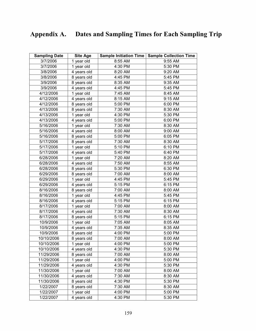
159

Appendix A. Dates and Sampling Times for Each Sampling Trip

Sampling Date Site Age Sample Initiation Time Sample Collection Time

3/7/2006 1 year old 8:55 AM 9:55 AM

3/7/2006 1 year old 4:30 PM 5:30 PM

3/8/2006 4 years old 8:20 AM 9:20 AM

3/8/2006 8 years old 4:45 PM 5:45 PM

3/9/2006 8 years old 8:35 AM 9:35 AM

3/9/2006 4 years old 4:45 PM 5:45 PM

4/12/2006 1 year old 7:45 AM 8:45 AM

4/12/2006 4 years old 8:15 AM 9:15 AM

4/12/2006 8 years old 5:00 PM 6:00 PM

4/13/2006 8 years old 7:30 AM 8:30 AM

4/13/2006 1 year old 4:30 PM 5:30 PM

4/13/2006 4 years old 5:00 PM 6:00 PM

5/16/2006 1 year old 7:30 AM 8:30 AM

5/16/2006 4 years old 8:00 AM 9:00 AM

5/16/2006 8 years old 5:00 PM 6:05 PM

5/17/2006 8 years old 7:30 AM 8:30 AM

5/17/2006 1 year old 5:10 PM 6:10 PM

5/17/2006 4 years old 5:40 PM 6:40 PM

6/28/2006 1 year old 7:20 AM 8:20 AM

6/28/2006 4 years old 7:50 AM 8:55 AM

6/28/2006 8 years old 5:30 PM 6:30 PM

6/29/2006 8 years old 7:00 AM 8:00 AM

6/29/2006 1 year old 4:45 PM 5:45 PM

6/29/2006 4 years old 5:15 PM 6:15 PM

8/16/2006 8 years old 7:00 AM 8:00 AM

8/16/2006 1 year old 4:45 PM 5:45 PM

8/16/2006 4 years old 5:15 PM 6:15 PM

8/17/2006 1 year old 7:00 AM 8:00 AM

8/17/2006 4 years old 7:30 AM 8:30 AM

8/17/2006 8 years old 5:15 PM 6:15 PM

10/9/2006 1 year old 7:05 AM 8:05 AM

10/9/2006 4 years old 7:35 AM 8:35 AM

10/9/2006 8 years old 4:00 PM 5:00 PM

10/10/2006 8 years old 7:00 AM 8:00 AM

10/10/2006 1 year old 4:00 PM 5:00 PM

10/10/2006 4 years old 4:30 PM 5:30 PM

11/29/2006 8 years old 7:00 AM 8:00 AM

11/29/2006 1 year old 4:00 PM 5:00 PM

11/29/2006 4 years old 4:30 PM 5:30 PM

11/30/2006 1 year old 7:00 AM 8:00 AM

11/30/2006 4 years old 7:30 AM 8:30 AM

11/30/2006 8 years old 4:30 PM 5:30 PM

1/22/2007 8 years old 7:30 AM 8:30 AM

1/22/2007 1 year old 4:00 PM 5:00 PM

1/22/2007 4 years old 4:30 PM 5:30 PM

160

1/23/2007 1 year old 7:30 AM 8:30 AM

1/23/2007 4 years old 8:00 AM 9:00 AM

1/23/2007 8 years old 4:00 PM 5:00 PM

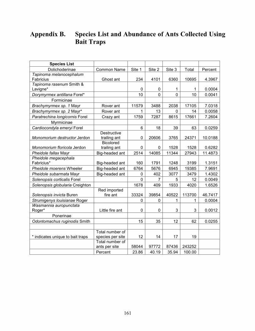
161

Appendix B. Species List and Abundance of Ants Collected Using

Bait Traps

Species List

Dolichoderinae Common Name Site 1 Site 2 Site 3 Total Percent

Tapinoma melanocephalum Fabricius Ghost ant 234 4101 6360 10695 4.3967

Tapinoma rasenum Smith & Lavigne* 0 0 1 1 0.0004

Dorymyrmex antillana Forel* 10 0 0 10 0.0041

Formicinae

Brachymyrmex sp. 1 Mayr Rover ant 11579 3488 2038 17105 7.0318

Brachymyrmex sp. 2 Mayr* Rover ant 1 13 0 14 0.0058

Paratrechina longicornis Forel Crazy ant 1759 7287 8615 17661 7.2604

Myrmicinae

Cardiocondyla emeryi Forel 6 18 39 63 0.0259

Monomorium destructor Jerdon Destructive trailing ant 0 20606 3765 24371 10.0188

Monomorium floricola Jerdon Bicolored trailing ant 0 0 1528 1528 0.6282

Pheidole fallax Mayr Big-headed ant 2514 14085 11344 27943 11.4873

Pheidole megacephala Fabricius* Big-headed ant 160 1791 1248 3199 1.3151

Pheidole moerens Wheeler Big-headed ant 6764 5676 6945 19385 7.9691

Pheidole subarmata Mayr Big-headed ant 0 402 3077 3479 1.4302

Solenopsis corticalis Forel 0 7 5 12 0.0049

Solenopsis globularia Creighton 1678 409 1933 4020 1.6526

Solenopsis invicta Buren Red imported

fire ant 33324 39854 40522 113700 46.7417

Strumigenys louisianae Roger 0 0 1 1 0.0004

Wasmannia auropunctata Roger* Little fire ant 0 0 3 3 0.0012

Ponerinae

Odontomachus ruginodis Smith 15 35 12 62 0.0255

* indicates unique to bait traps Total number of species per site 12 14 17 19

Total number of ants per site 58044 97772 87436 243252

Percent 23.86 40.19 35.94 100.00

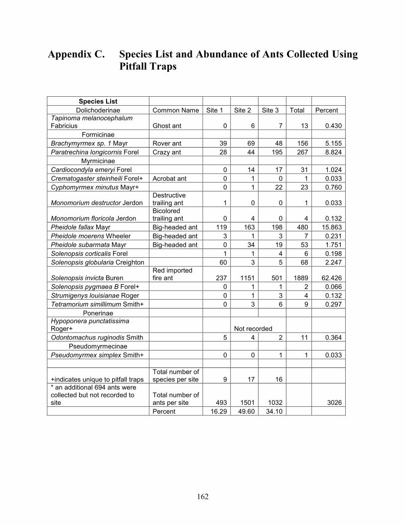
162

Appendix C. Species List and Abundance of Ants Collected Using

Pitfall Traps

Species List

Dolichoderinae Common Name Site 1 Site 2 Site 3 Total Percent

Tapinoma melanocephalum Fabricius Ghost ant 0 6 7 13 0.430

Formicinae

Brachymyrmex sp. 1 Mayr Rover ant 39 69 48 156 5.155

Paratrechina longicornis Forel Crazy ant 28 44 195 267 8.824

Myrmicinae

Cardiocondyla emeryi Forel 0 14 17 31 1.024

Crematogaster steinheili Forel+ Acrobat ant 0 1 0 1 0.033

Cyphomyrmex minutus Mayr+ 0 1 22 23 0.760

Monomorium destructor Jerdon Destructive trailing ant 1 0 0 1 0.033

Monomorium floricola Jerdon Bicolored trailing ant 0 4 0 4 0.132

Pheidole fallax Mayr Big-headed ant 119 163 198 480 15.863

Pheidole moerens Wheeler Big-headed ant 3 1 3 7 0.231

Pheidole subarmata Mayr Big-headed ant 0 34 19 53 1.751

Solenopsis corticalis Forel 1 1 4 6 0.198

Solenopsis globularia Creighton 60 3 5 68 2.247

Solenopsis invicta Buren Red imported fire ant 237 1151 501 1889 62.426

Solenopsis pygmaea B Forel+ 0 1 1 2 0.066

Strumigenys louisianae Roger 0 1 3 4 0.132

Tetramorium simillimum Smith+ 0 3 6 9 0.297

Ponerinae

Hypoponera punctatissima Roger+ Not recorded

Odontomachus ruginodis Smith 5 4 2 11 0.364

Pseudomyrmecinae

Pseudomyrmex simplex Smith+ 0 0 1 1 0.033

+indicates unique to pitfall traps Total number of species per site 9 17 16

* an additional 694 ants were collected but not recorded to site

Total number of ants per site 493 1501 1032 3026

Percent 16.29 49.60 34.10

Documents

Spatiotemporal Composition of Pest Ant Species in the ... · (RIFA). Fourteen different species were identified from the one-year-old site. However, RIFA ... Mullins for always having