An Invitation to Spatio-Temporal Data Miningweb.cs.iastate.edu/~honavar/Seminars/Fall04/spatio-temporal-datamining.pdfAn Invitation to Spatio-Temporal Data Mining Deﬁnition and Applications

An Invitation to Spatio-TemporalData Mining

Definition and Applications

Sanjay Chawla

School of Information Technologies

University of Sydney

An Invitation to Spatio-Temporal Data Mining – p.1

http://www.it.usyd.edu.au/

Data Mining and the Indian Monsoon

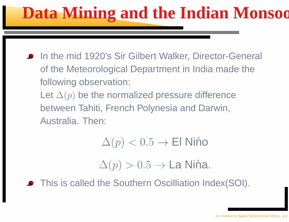
In the mid 1920’s Sir Gilbert Walker, Director-Generalof the Meteorological Department in India made thefollowing observation:Let

� ��

be the normalized pressure differencebetween Tahiti, French Polynesia and Darwin,Australia. Then:

� �� El Nino

� �� La Nina�

This is called the Southern Oscilliation Index(SOI).


Data Mining & Indian Mons’n(Contd.)

El Nino corresponds to a dry spell in Indiaand Australia.

Contrast this with fictitious diaper-beerexample.


Other Theories Using Spatial Data

Dr. Snow and Cholera Map: Plot location of cholera patients;

Centroid water pump; Disease subsides by turning-off the pump.

Flouride and Dental Health: Residents of Colorado Springs had

unusually healthy teeth; Flouride present in groundwater.

Theory of Gondwanaland: All continents formed one land mass.

Locating the Severe Accute Respiratory Syndrome(SARS) Index

Patient: The people who carried the disease to Vietnam,

Singapore and Toronto all stayed on the 9th floor of the Metropolis

hotel in Hong Kong.


Data Mining Trinity

Regression and Classification: Explain onevariable in terms of others.

Clustering: Segmentation; Categorize datapoints into a few “meaningfull” groups- likeSoccer Moms. Includes outlier detection.

Association Rules: Discover rules of the form

� � �

from transaction databases.


Spatial and Temporal Autocorrelation

"All things are related but nearby things aremore related than distant things" – Tobler’sFirst Law of Geography.

Similarly events are related in time. Forexample,

Temperature and pressure have bothspatial and temporal correlation.People with similar lifestyle tend togravitate towards similar neighborhoods.


Spatio-Temporal Data Mining

Incorporate spatio-temporal autocorrelationinto standard data mining techniques likeregression, classification, clustering andassociation rules.


Moran I : Measure of SA

Contiguity Matrix

B

C

DCBADCBA

D D

C

AA

B 1

1

1

1B

C D

01

A

00

(b) Boolean W

0

0

0

0.3

1

0

0 0

0.30.3

0 0.50.5

00.50.5

(c) Row-normalized W(a) Map

10

010

010


Moran I: Measure of SA (Contd.)

Given a variable � � � ��

sampled over nlocations. The Moran I coefficient is defined as

� ��

� � �where � � � ��

, where

� � is the mean of

� and

is the � � � row-normalized contiguity matrix.

� ��

��

� � �

positive autocorrelation

� � �negative autocorrelation

� �no autocorrelation detected


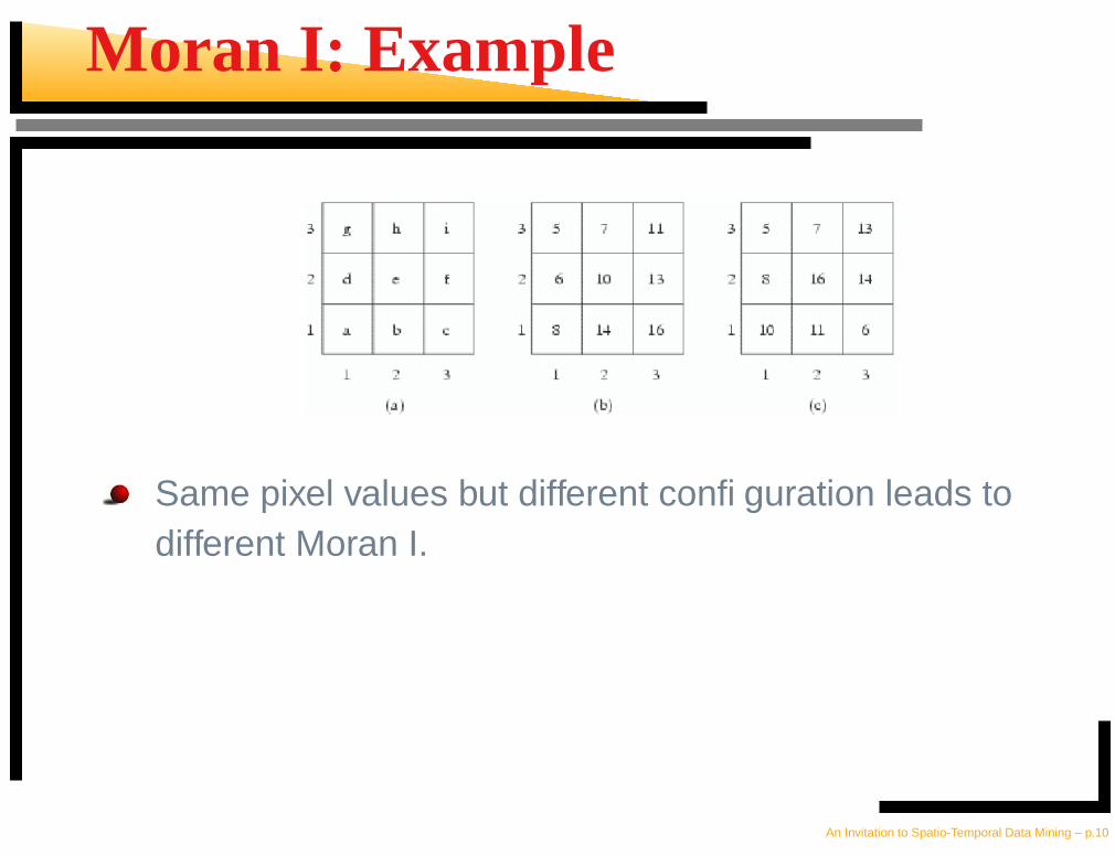
Moran I: Example

Same pixel values but different configuration leads todifferent Moran I.


Spatial Autogressive Regression

General Linear Regression Equation

� � � �� where � � � �� is i.i.d

Now if � is SA then that is not being capturedin the model.

This can be tested by calculating the Moran Iin the error term �.Will lead to lower

� �

.


The SAR model

First-order correction: � � � ��

Let’s derive the solution for slightly simpler

� � � �� where � � � � ��

.

Given data and assuming normal distributionfind parameters of the distribution.


The SAR model (Contd.)

� ��

� � � ��

For us

� � � � �

. Now, � � � � � � � � � � � �� . Thus

��

� ��

Therefore the probability density of � is

� � ��

�


SAR (Contd.)

Expanding,

��

��

Now

� � � � � � � � � � � �� therefore the likelihood

�

is

� � ��

� � ��

The likelihood is the pdf but as a function of the parameters.

Want to maximize�

, so can maximize the log-likelihood

� �

��

.


SAR (Contd.)

� � � ��

��

� � �

� � � � � �

Calculating the determinant is the hard part. Notice thesimilarity between

� � � � �

and the characteristicpolynomial of

,

� � �

.If

�� are the eigenvalues of the

then

� � � � � ��

��


SAR (Contd.)

Setting

� �

and noting � � � is an eigenvalue of � we get

� � � � � � � � � �The problem has been reduced to calculating the eigenval-

ues of a sparse banded matrix


SAR Example

Dataset 4 variables on 3107 US counties

Dependent Number of voters in each county

Independent Education, Homeownership and Income

Method

� �

Moran I(residuals)OLS a 0.4635 0.4377SAR 0.6356 0.0272

aOrdinary Least Square


Spatio-Temporal Clustering & Classification

Spatio-Temporal clustering is “equivalent” totracking of moving objects, especially inimages.

First we want to classify objects in images.Then track objects in time.


MRF and Kalman Filtering

Markov Random Fields(MRF) for classifying objects inspace.

Kalman Filtering for tracking objects in time.

MRF and its solution as a combinatorial optimizationproblem.

Followed by an informal introduction to KalmanFiltering


Spatial Clustering and Classification

MRF’s were introduced by Geman and Geman forimage restoration.

Images are typically piece-wise smooth.

We want the data mining method to learn “discontinuitypreserving functions”.


Bayes Theorem

Let

�

and

�

be events in a sample space thenBayes Theorem says

� � � � � ��

� � �


Bayesian Classification : Example

Lets do the famous “tennis” example to showhow Baye’s theorem is used in classification.

outlook(O) temp(T) humidity(H) windy(W) play(PL)

sunny hot high false no

rainy mild high true yes

: : : : :overcast cool high true ?


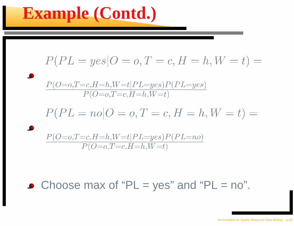
Example (Contd.)

� � ��

��

��

� � ��

��

��

Choose max of “PL = yes” and “PL = no”.


Graph Partitioning and Classification

L1 L2

yes no

0.7

0.3

.0.4

0.6

.55

0.45

L3 L1 L2

yes no

0.7 .0.6

.55

L3

Definition: A k-cut set is a set of edges whose removal

partitions the graph into

�

components.

Example: The edges

� � ��

� ��

� � ��

is a 2-cut

set which isolates the nodes

� � �� .

Example: Maximum a posteriori estimate corresponds to a min-

cut partitoning of the above graph.An Invitation to Spatio-Temporal Data Mining – p.24

Graph Partitioning and Spatial Classification

L1 L2

yes no

0.7

0.3

.0.4

0.6

.55

0.45

L30.2 0.2

L1 L2

yes no

0.7 .0.4

0.45

L30.2

Example: The edges� � � � ��

��

��

��

is a min-cut set. Note how the inclusion of spatial context

changes the min-cut set.


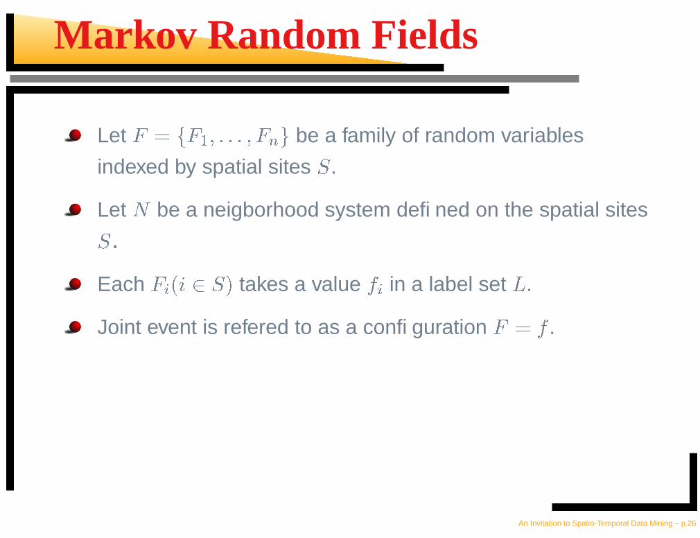
Markov Random Fields

Let

� � � ��

��

be a family of random variables

indexed by spatial sites

�

.

Let

�

be a neigborhood system defined on the spatial sites

�.

Each

� � ��

takes a value

� in a label set

�

.

Joint event is refered to as a configuration

� �

.


Markov Random Fields (Contd.)

The joint probability is denoted by� ��

.

�

is a Markov Random Field (MRF) provided

� ��

� ��


Hammersley-Clifford Theorem

� ��

� ��

� � is the clique potential

Want to choose

�

which maximizes

� ��

, where

�

is the data

From Bayes Theorem

� ��



Use conditional independence

� � � � � � � � � � � � � � � � � � � � Assume Gaussian Distribution

� � � � � � � � � ��

�� Now

� ��

��

� ��

Maximizing is equivalent to minimizing thenegative log.



Thus, we want an

�

which minimizes

� � � � � � ��

� �

��

� � ��

The Potts model assumes that

� � � � ��

where

�

is the dirac delta function.


Results of Boykov, Vekslar and Zabih

Minimizing the Potts energy is NP-hard.

Minimizing the Potts Energy can be solved bycomputing the minimum cost multiway cut on certaingraph.

BVZ propose two algorithms: Swap(when

�

is ametric) and Expansion(when

�

is a semi-metric) whichcomputes a 2-approximate local minima, i.e., if

� �

isthe solution from their algorithm and

��

is the globalminima then

� ��


Results of the MRF Model


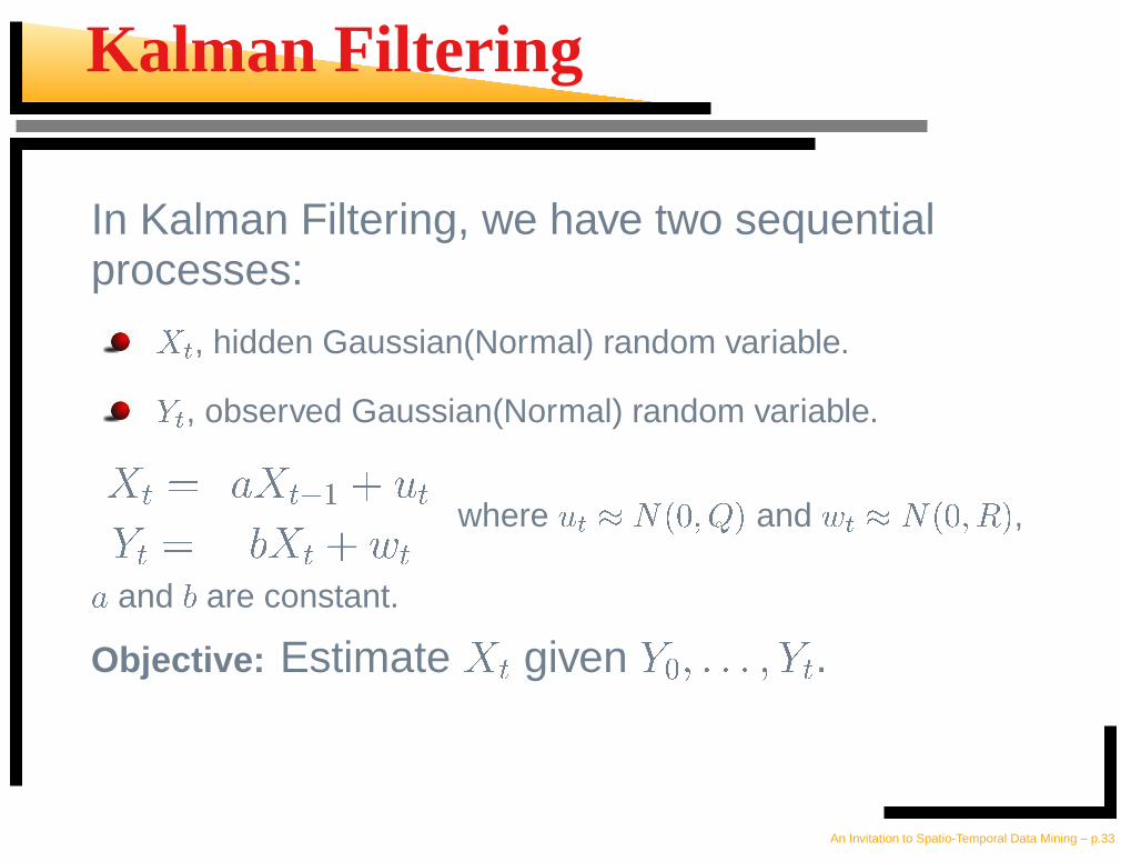
Kalman Filtering

In Kalman Filtering, we have two sequentialprocesses:

� �, hidden Gaussian(Normal) random variable.

� �, observed Gaussian(Normal) random variable.

� � � � � � � � � � �

� � � � � � � � � where � � � ��

� �

and � � � ��

�

,

� and

�

are constant.

Objective: Estimate� � given

�� .


Brief Derivation of Kalman Equations

1. Guess

�� and the variance

� � � � � � � � ��

.

2. Our best estimate of

�� ;

�� .

3.

� ��

� ��

4. Now,

�� .


Derivation (Contd.)

5.

� � � � ��

; K is Kalman Gain?

6. Choose

�

to minimize

� � � � � � ��

7.

� � � � ��

8.

� � �� 9. Set

�� Goto step 2.


Kalman Filtering : Example

� � � � ��

� � � � ��

0.

��

1.

� �� 2.

� ��

3.

� � ��

� � � � � �� 4.

� � � � � ��

5.

�� and� � � �. Goto step 1.


Kalman Example (Contd)

0 10 20 30 40 50 60 70 80 90 10020

40

60

80

100

120

140

Time

Value

s

Kalman Filtering

true valuesobserved valuesestimtated values


Combining MRF & Kalman Filtering

Clustering of spatio-temporal images(data) isequivalent to tracking of moving objects.

Given an image at time

� � , first identify theobjects in the image(for e.g., using an MRFmodel) and then track the objects into thenext time frame(

� �

) using Kalman Filtering.

Requires the calculation of motion vectorsfrom one time frame into the next.


Example of Spatio-Temporal Clustering

[Authors:Kamijo, Ikeuchi and Sakauchi]


Example of Spatio-Temporal Clustering (Contd.)

[Authors:Kamijo, Ikeuchi and Sakauchi]


Summary

Spatio-Temporal clustering is equivalent todetecting and tracking of spatial movingobjects.

MRF is a rigorous method for incorporatingspatial context.

Kalman Filtering for can be used for trackingobjects in time.

Some work has been done on combining thetwo.


Spatial Association Rules

Association rules are probably the most researchedform of “patterns” within data mining.

Framed in market basket analysis:"Given collection of items

�

. Let�

� � � �

. A rule is animplication of the form

� � �."

The support of the rule� � �

is

� � ��

and itsconfidence is

� � � � � �. Association rules are all those

rules which satisfy minsupport and minconfidence.

How can association rules be adapted for spatial data?


Apriori algorithm to mine association rules

Key Challenge Large Search Space:

� �frequent items.

Key Assumption Low support rules are “uninteresting”.

Key Insight Subsets of frequent itemsets are

frequent.

Details 1. Find all frequent itemsets.

2. Generate association rules with

confidence above minconfidence.


Apriori Algorithm

Uses a level-wise approach to mine frequentitemsets from transactional databases.

First finds all frequent level 1 itemsets,

� �

.Then uses

� �

to find frequent level 2itemsets,

� �

. Proceeds until no more higherlevel itemsets can be found.


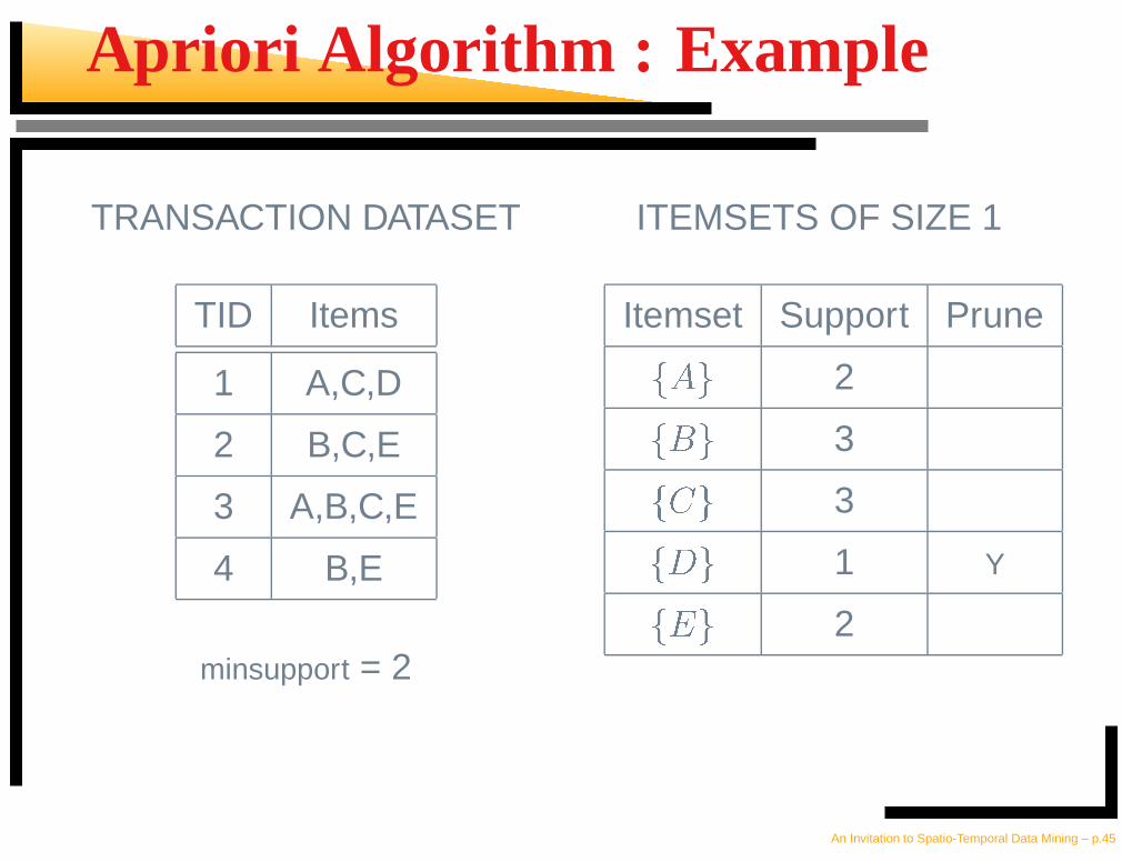
Apriori Algorithm : Example

TRANSACTION DATASET

TID Items

1 A,C,D

2 B,C,E

3 A,B,C,E

4 B,E

minsupport = 2

ITEMSETS OF SIZE 1

Itemset Support Prune

� � 2

� � 3

� �

3

��

1 Y

� �

2


Apriori Algorithm : Example (Contd.)

ITEMSETS OF SIZE 2


� ��

1 Y

� ��

�

2

� ��

1 Y

� ��

�

2

� ��

3

� ��

2

ITEMSETS OF SIZE 3


� ��

� 1 Y

� ��

��

1 Y

� ��

��

2

Apriori Terminates


Colocation Rules

MotivationAssociation rules need transactionsSpatial data is “continuous”Decomposing spatial data into transactionsmay alter patterns


Colocation Rules (Contd.)

For point data in space

Work directly with continuous space

Use neighborhoods and spatial joins

“Natural approach”


Cliques and Colocation Rules

Given two features maps

�

and

�

. Let��

and

�� be instances(items) of the two

features. Then these two instances co-locateif

� � ��

� for some pre-definedthreshold �.

A clique

�

is set of features instances suchthat if

�

and

�

belong to

�

then

�

and

�

co-locate.


Colocation Rules vs. Association Rules

Association Rules assume that a finite set oftransactions is given as input to the algorithm.For spatial features there is no explicit set oftransactions.

For the co-location problem, transactions aredefined as instances of cliques.


Colocation Patterns : Example

No Clique

1

� ��

2

��

� �

3

��

��

4

� �

� � ��

5

� � �

��

� �

6

� � �

� � �

��

7

� ��

8

� �

9

� � �

10

� � �

� �

�

D5

D2 A4

C 1

D1C 5 C 6

A1 B1

C 2

B 2

D4

A2

C 3 D3

D6A5

C 4

A3B 3


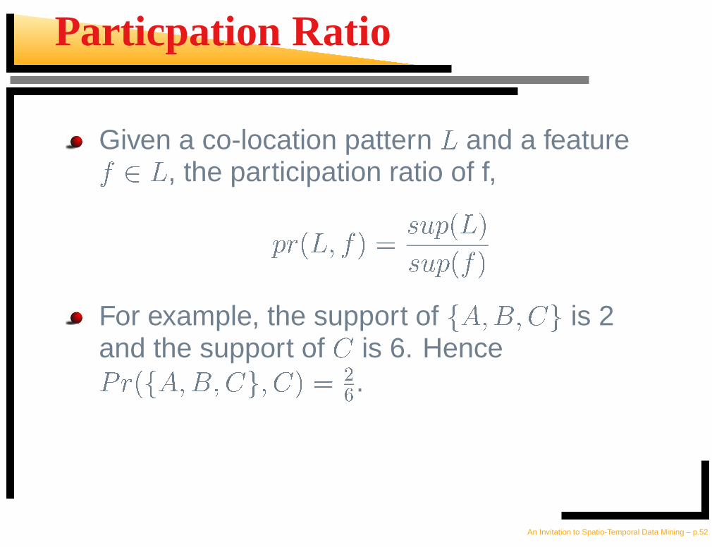
Particpation Ratio

Given a co-location pattern

�

and a feature� � � , the participation ratio of f,

� � � � � � � � ��

� ��

For example, the support of

� ��

is 2and the support of

�is 6. Hence

� � � � �� .


Minimal Participation Index

Given a co-location pattern

�

, the minimalparticipation index of

�

, � � � �� is defined

as

� � � ��

� � � � � � � �

For example,

� � � � � � � ��

� �

= � � � ��

� �

� ��

� � � ��

��

� �

� � �

= � � � ��


Monotonic Property of minPI

minPI is monotonic w.r.t. to the patterncontainment relation

If

�

is a k-co-location pattern, the minPI of all��

sub-patterns of

� � � � � ��

So, we can use minPI instead of support aspruning metric in the Apriori algorithm


Weakness of MinPI

Same weakness as the support metric. Sometimeslow-frequency but confidence rules are interesting.

Suppose

�

and

�

are two spatial features. Thesupport of

�

is 100 and the support of

�

is 10. Usingclique generation, found 10 instances of

� ��

. Then

� � �

is 100% confidence rule.

But � � � � � � ��

.Thus relatively low minPI.

Think Erin Bronkovich!


Maximal Participation Index

The maximal participation ratio,

� � � ��

For example,

� � � � � � ��

� �

= � � ��

� �

� �

� ��

� � � �

�

��

� �

� � �

= � � � ��


Weak monotonic property of maxPI

maxPI is weakly monotonic with respect to the patterncontainment relation.

If P is a k-co-location pattern, then there exists at mostone

��

subpattern

� � � �

such that

� � � � � � � � � � � � � � � �

.

Thus if � � � � � ��

� � � � and � � � � � ��

� � � � but

� � � � � �� .

� �� will be pruned but

� ��

�

can be recovered from� ��

�

and

� ��

�

.

Modify Apriori to get use maxPI and recover rare buthigh-confidence rules.


Clique Generation

Suppose we have

�

A’s and B’sdistributed in

� ��

space. What’s thecomplexity of generating all

� ��

cliques?

Normally, we have to compute the distancebetween each instance of

�and

�

. Thecomplexity of this is

� � � �

.

Can use a Quarternary tree index to generatecliques.


Quaternary Tree Indexing

Similar to B+ index, but each node has only fourchildren.

As the root note of the tree, we use a large rectangle that

covers all the points.

Then divide it into four equal-sized sub-rectangles.

Continue this division procedure recursively.

We set the depth of the quarternary tree so thataverage number of points in each small rectangle isclose to one.

The complexity of constructing the quarternary tree is

� �� .


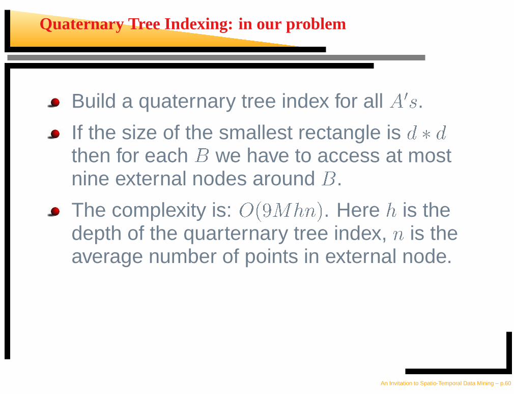
Quaternary Tree Indexing: in our problem

Build a quaternary tree index for all� � �.

If the size of the smallest rectangle is

� � �

then for each

�

we have to access at mostnine external nodes around

�.

The complexity is:

� �� . Here

�

is thedepth of the quarternary tree index, � is theaverage number of points in external node.


Notes

A detailed account of spatial statistics can be found in [4]. Spatial regression

techniques have been extensively has been extensively studied in [2].

James LeSage has also provided an excellent Matlab toolbox which implements

several algorithms for spatial regression.

The Apriori algoirthm was introduced by [1], and [8] report its first known extension

to spatial data.

[10] presented an efficient algorithm to mine a kind of spatial co-locations. The

concepts of neighborhood, participation ratio, participation index were defined.

Instead of support, the minimal participation index was used as a pruning measure

in the conventional Apriori-like technique.

A drawback of the minimal participation index is that some confident co-location

rules with low support are also pruned. In order to solve this problem, [5] proposed

the concept of a maximal participation index.


Notes...cont

For a description of the extension of regression and Bayesian methods to spatial

data (SAR, MRF) see [9].

[7] describes how energy functions can be minimized by graph cuts. Although the

results were restricted to energy functions with binary variables, they suggest the

extension to vision problems involving large numbers of labels, as is described in

[3].

In [6] it is proposed that a Spatio-Temporal Markov Random Field model for

segmentation of spatio-temporal images is appropriate for object tracking.

Refer to [11] For a general description(in book form) of spatial data mining issues.John Roddick et. al have compiled a comprehensive bibliography on

spatio-temporal data mining which is available at

http://kdm.first.flinders.edu.au/IDM/STDMBib.bib


References

[1] Rakesh Agrawal and Ramakrishnan Srikant. Fast algo-

rithms for mining association rules. In Jorge B. Bocca,

Matthias Jarke, and Carlo Zaniolo, editors, Proceedings

of 20th Int. Conf. Very Large Data Bases, VLDB, pages

487–499. Morgan Kaufmann, 1994.

[2] L. Anselin. Spatial Econometrics:Methods and Models.

Kluwer Academics, 1988.

[3] Yuri Boykov, Olga Veksler, and Ramin Zabih. Fast approx-

imate energy minimization via graph cuts. In ICCV (1),

pages 377–384, 1999.

[4] Noel A. Cressie. Statistics for Spatial Data. New York:

Wiley, 1993.

[5] Y. Huang, H. Xiong, and S. Shekhar. Mining confident

co-location rules without a support threshold. In Proceed-

ings of Athe 18th ACM Symposium on Applied Computing

(ACM SAC), 2003.

[6] Shunsuke Kamijo, Katsushi Ikeuchi, and Masao Sakauchi.

Segmentations of spatio-temporal images by spatio-

temporal markov random field model. In EMMCVPR En-

ergy Minimization Methods in Computer Vision and Pat-

tern Recognition, Third International Workshop,, pages

298–313, 2001.

62-1

[7] Vladimir Kolmogorov and Ramin Zabih. What energy

functions can be minimized via graph cuts? In ECCV

(3), pages 65–81, 2002.

[8] Krzysztof Koperski, Junas Adhikary, and Jiawei Han.

Knowledge discovery in spatial databases: Progress and

challenges. In ACM SIGMOD Workshop on Research Is-

sues on Data Mining and Knowledge Discovery, pages

55–70, Montreal, Canada, 1996.

[9] S. Shekhar, P. Schrater, R. Vatsavai, W. Wu, and

S. Chawla. Spatial contex- tual classification and predic-

tion models for mining geospatial data. In Proceedings of

IEEE Transaction on Multimedia, 2002.

[10] Shashi Shekhar and Yan Huang. Discovering spatial co-

location patterns: A summary of results. Lecture Notes in

Computer Science, 2121, 2001.

[11] S.Shekhar and S.Chawla. Spatial Databases:A Tour.

Prentice Hall, 2002.

62-2

Documents

An Invitation to Spatio-Temporal Data Miningweb.cs.iastate.edu/~honavar/Seminars/Fall04/spatio-temporal-datamining.pdfAn Invitation to Spatio-Temporal Data Mining Deﬁnition and Applications