Embed Size (px)
Citation preview
Introduction Fuel Distribution Model Parameter Estimation Spatial Distribution of D-S Gap Conclusion Appendix
Spatio-Temporal Analysis of GasolineShortage in Tohoku Region after the Great
East Japan Earthquake
Takashi AKAMATSU and Takeshi NAGAE(Tohoku University, Japan)
2 March, 2013
International Workshop on Transport Networks underHazardous Conditions
Introduction Fuel Distribution Model Parameter Estimation Spatial Distribution of D-S Gap Conclusion Appendix
Outline
1 Introduction
2 Fuel Distribution Model
3 Parameter Estimation
4 Spatial Distribution of D-S Gap
5 Conclusion
6 Appendix
Introduction Fuel Distribution Model Parameter Estimation Spatial Distribution of D-S Gap Conclusion Appendix
Outline
1 Introduction
2 Fuel Distribution Model
3 Parameter Estimation
4 Spatial Distribution of D-S Gap
5 Conclusion
6 Appendix
Introduction Fuel Distribution Model Parameter Estimation Spatial Distribution of D-S Gap Conclusion Appendix
Motivation
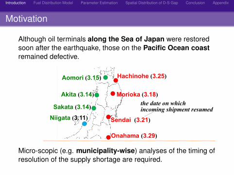
Although oil terminals along the Sea of Japan were restoredsoon after the earthquake, those on the Pacific Ocean coastremained defective.Damages to Major Oil Terminals in Tohoku
7
Niigata (3.11)
Sakata (3.14)
Akita (3.14)
Aomori (3.15) Hachinohe (3.25)
Morioka (3.18)
Sendai (3.21)
Onahama (3.29)3.11 – 3.13: all oil terminals (except Niigata) are inoperable3.14 – 3.21: terminals on the Pacific Ocean are inoperable;
only the terminals on the Japan Sea are operable.3.21 - : the Pacific terminals gradually resume
the date on which incoming shipment resumed
Micro-scopic (e.g. municipality-wise) analyses of the timing ofresolution of the supply shortage are required.
Introduction Fuel Distribution Model Parameter Estimation Spatial Distribution of D-S Gap Conclusion Appendix
Purpose
Develop a model for estimating the spatio-temporaldistribution of demand-supply (D-S) gap, which consists of
1. Inter-temporal dynamics of fuel demand withdisappearance due to a huge backlog
2. Intra-temporal fuel assignments taking into account thefairness among municipalities.
Estimate model parameters and obtain spatio-temporaldistributions of D-S gap.
Introduction Fuel Distribution Model Parameter Estimation Spatial Distribution of D-S Gap Conclusion Appendix
Outline
1 Introduction
2 Fuel Distribution Model
3 Parameter Estimation
4 Spatial Distribution of D-S Gap
5 Conclusion
6 Appendix
Introduction Fuel Distribution Model Parameter Estimation Spatial Distribution of D-S Gap Conclusion Appendix
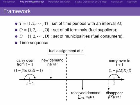
Framework
T = {1, 2, · · · ,T} : set of time periods with an interval ∆t;O = {1, 2, · · · ,O} : set of oil terminals (fuel suppliers);D = {1, 2, · · · ,D} : set of municipalities (fuel consumers).Time sequence
t − 1 t
fuel assignment at t
carry overfrom t − 1
(1 − β∆t)X j(t − 1)
new demandr j(t)∆t
resolved demand∑i∈O xi j(t)
(1 − β∆t)X j(t)
carry over tot + 1
disappearβX(t)∆t
Introduction Fuel Distribution Model Parameter Estimation Spatial Distribution of D-S Gap Conclusion Appendix
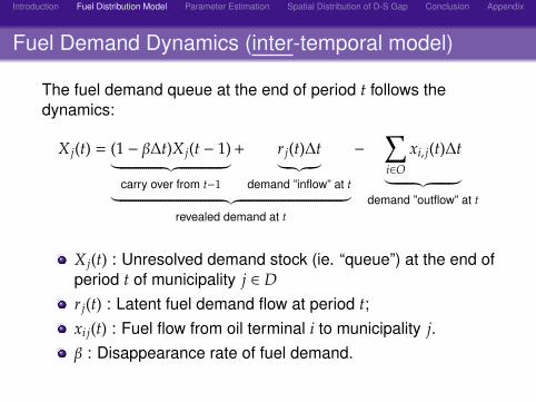
Fuel Demand Dynamics (inter-temporal model)
The fuel demand queue at the end of period t follows thedynamics:
X j(t) = (1 − β∆t)X j(t − 1)︸ ︷︷ ︸carry over from t−1
+ r j(t)∆t︸ ︷︷ ︸demand ”inflow” at t︸ ︷︷ ︸
revealed demand at t
−∑i∈O
xi, j(t)∆t︸ ︷︷ ︸demand ”outflow” at t
X j(t) : Unresolved demand stock (ie. “queue”) at the end ofperiod t of municipality j ∈ Dr j(t) : Latent fuel demand flow at period t;xi j(t) : Fuel flow from oil terminal i to municipality j.β : Disappearance rate of fuel demand.
Introduction Fuel Distribution Model Parameter Estimation Spatial Distribution of D-S Gap Conclusion Appendix
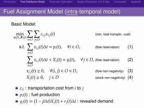
Fuel Assignment Model (intra-temporal model)
Basic Model:
minx(t),X(t)
∑i∈O
∑j∈D
ci, jxi, j(t) (min. total transptn. cost)
s.t.∑j∈D
xi, j(t)∆t = pi(t), ∀i ∈ O, (flow reservation) (1)∑i∈O
xi, j(t)∆t + X j(t) = qi(t), ∀ j ∈ D, (flow reservation) (2)
xi, j(t) ≥ 0, ∀(i, j) ∈ O ×D, (flow non-negativity) (3)X j(t) ≥ 0, j ∈ D (stock non-negativity) (4)
ci j : transportation cost from i to jpi(t) : fuel productionq j(t) B (1 − β∆t)X j(t) + r j(t)∆t : revealed demand
Introduction Fuel Distribution Model Parameter Estimation Spatial Distribution of D-S Gap Conclusion Appendix
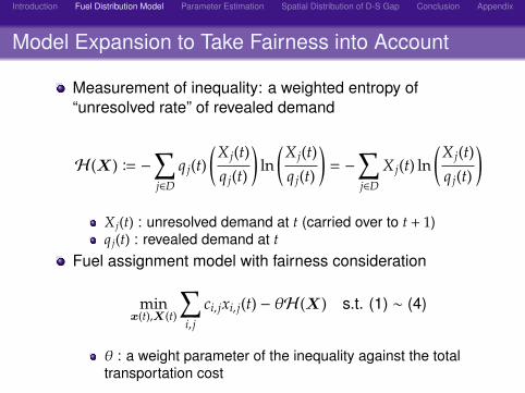
Model Expansion to Take Fairness into Account
Measurement of inequality: a weighted entropy of“unresolved rate” of revealed demand
H(X) B −∑j∈D
q j(t)(
X j(t)q j(t)
)ln
(X j(t)q j(t)
)= −
∑j∈D
X j(t) ln(
X j(t)q j(t)
)
X j(t) : unresolved demand at t (carried over to t + 1)q j(t) : revealed demand at t
Fuel assignment model with fairness consideration
minx(t),X(t)
∑i, j
ci, jxi, j(t) − θH(X) s.t. (1) ∼ (4)
θ : a weight parameter of the inequality against the totaltransportation cost
Introduction Fuel Distribution Model Parameter Estimation Spatial Distribution of D-S Gap Conclusion Appendix
Outline
1 Introduction
2 Fuel Distribution Model
3 Parameter Estimation
4 Spatial Distribution of D-S Gap
5 Conclusion
6 Appendix
Introduction Fuel Distribution Model Parameter Estimation Spatial Distribution of D-S Gap Conclusion Appendix
Parameter Estimation I
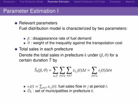
Relevant parametersFuel distribution model is characterized by two parameters:
β : disappearance rate of fuel demandθ : weight of the inequality against the transpotation cost
Total sales in each prefectureDenote the total sales in prefecture k under (β, θ) for acertain duration T by
Sk(β, θ) =∑t∈T
∑j∈Dk
∑i∈O
xi, j(t)∆t =∑j∈Dk
s j(t)∆tn
s j(t) B∑
i∈O xi, j(t): fuel sales flow in j at period t;Dk : set of municipalities in prefecture k.
Introduction Fuel Distribution Model Parameter Estimation Spatial Distribution of D-S Gap Conclusion Appendix
Parameter Estimation II
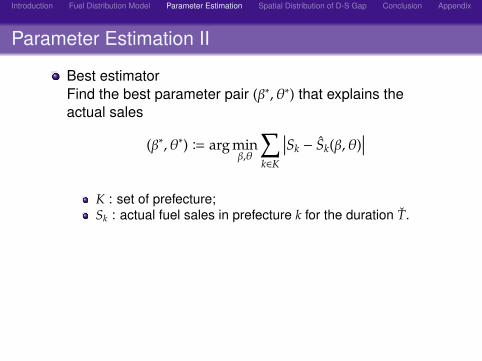
Best estimatorFind the best parameter pair (β∗, θ∗) that explains theactual sales
(β∗, θ∗) B arg minβ,θ
∑k∈K
∣∣∣Sk − Sk(β, θ)∣∣∣
K : set of prefecture;Sk : actual fuel sales in prefecture k for the duration T.
Introduction Fuel Distribution Model Parameter Estimation Spatial Distribution of D-S Gap Conclusion Appendix
Data
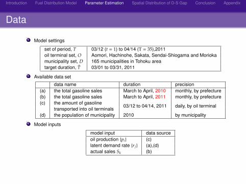
Model settings
set of period, T 03/12 (t = 1) to 04/14 (T = 35),2011oil terminal set, O Aomori, Hachinohe, Sakata, Sendai-Shiogama and Moriokamunicipality set, D 165 municipalities in Tohoku areatarget duration, T 03/01 to 03/31, 2011
Available data set
data name duration precision(a) the total gasoline sales March to April, 2010 monthly, by prefecture(b) the total gasoline sales March to April, 2011 monthly, by prefecture(c) the amount of gasoline
03/12 to 04/14, 2011 daily, by oil terminaltransported into oil terminals
(d) the population of municipality 2010 by municipality
Model inputs
model input data sourceoil production {pi} (c)latent demand rate {r j} (a),(d)actual sales Sk (b)
Introduction Fuel Distribution Model Parameter Estimation Spatial Distribution of D-S Gap Conclusion Appendix
Estimated Parameters
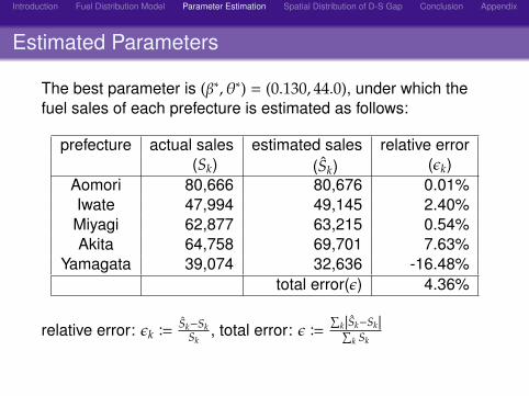
The best parameter is (β∗, θ∗) = (0.130, 44.0), under which thefuel sales of each prefecture is estimated as follows:
prefecture actual sales estimated sales relative error(Sk) (Sk) (ϵk)
Aomori 80,666 80,676 0.01%Iwate 47,994 49,145 2.40%Miyagi 62,877 63,215 0.54%Akita 64,758 69,701 7.63%
Yamagata 39,074 32,636 -16.48%total error(ϵ) 4.36%
relative error: ϵk BSk−Sk
Sk, total error: ϵ B
∑k|Sk−Sk|∑
k Sk
Introduction Fuel Distribution Model Parameter Estimation Spatial Distribution of D-S Gap Conclusion Appendix
Outline
1 Introduction
2 Fuel Distribution Model
3 Parameter Estimation
4 Spatial Distribution of D-S Gap
5 Conclusion
6 Appendix
Introduction Fuel Distribution Model Parameter Estimation Spatial Distribution of D-S Gap Conclusion Appendix
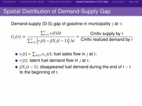
Spatial Distribution of Demand-Supply Gap
Demand-supply (D-S) gap of gasoline in municipality j at τ:
G j(τ) B
∑τt=1 s j(t)∆t∑τ
t=1
{r j(t) − βX j(t − 1)
}∆t=
Cmltv supply by tCmltv realized demand by t
s j(t) =∑
i∈O xi, j(t): fuel sales flow in j at t;r j(t): latent fuel demand flow in j at t;βX j(t − 1): disappeared fuel demand during the end of t − 1to the beginning of t.
Introduction Fuel Distribution Model Parameter Estimation Spatial Distribution of D-S Gap Conclusion Appendix
Spatio-Temporal Distribution of D-Sn Gap (summary)
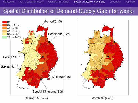
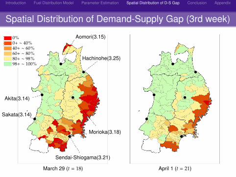
The subsequent 3 slides show:1. It was hard to resolve the D-S gap in the areas along the
Pacific Sea. Especially, even 3 weeks after the earthquake,the D-S gaps remained in Miyagi and Iwate, whereas thosein other prefectures were almost resolved;
2. At each day, the D-S gap was greater in theeastern-southern regions compared to thewestern-northern regions.
Introduction Fuel Distribution Model Parameter Estimation Spatial Distribution of D-S Gap Conclusion Appendix
Spatial Distribution of Demand-Supply Gap (1st week)
"
"
"
"
"
"
0%0+ ∼ 40%40+ ∼ 60%60+ ∼ 80%80+ ∼ 98%98+ ∼ 100%
Aomori(3.15)
Hachinohe(3.25)
Akita(3.14)
Morioka(3.18)
Sendai-Shiogama(3.21)
Sakata(3.14)
March 15 (t = 4) March 18 (t = 7)

Introduction Fuel Distribution Model Parameter Estimation Spatial Distribution of D-S Gap Conclusion Appendix
Spatial Distribution of Demand-Supply Gap (2nd wk)
"
"
"
"
"
"
0%0+ ∼ 40%40+ ∼ 60%60+ ∼ 80%80+ ∼ 98%98+ ∼ 100%
Aomori(3.15)
Hachinohe(3.25)
Akita(3.14)
Morioka(3.18)
Sendai-Shiogama(3.21)
Sakata(3.14)
March 22 (t = 11) March 25 (t = 14)
Introduction Fuel Distribution Model Parameter Estimation Spatial Distribution of D-S Gap Conclusion Appendix
Spatial Distribution of Demand-Supply Gap (3rd week)
"
"
"
"
"
"
0%0+ ∼ 40%40+ ∼ 60%60+ ∼ 80%80+ ∼ 98%98+ ∼ 100%
Aomori(3.15)
Hachinohe(3.25)
Akita(3.14)
Morioka(3.18)
Sendai-Shiogama(3.21)
Sakata(3.14)
March 29 (t = 18) April 1 (t = 21)
Introduction Fuel Distribution Model Parameter Estimation Spatial Distribution of D-S Gap Conclusion Appendix
Outline
1 Introduction
2 Fuel Distribution Model
3 Parameter Estimation
4 Spatial Distribution of D-S Gap
5 Conclusion
6 Appendix
Introduction Fuel Distribution Model Parameter Estimation Spatial Distribution of D-S Gap Conclusion Appendix
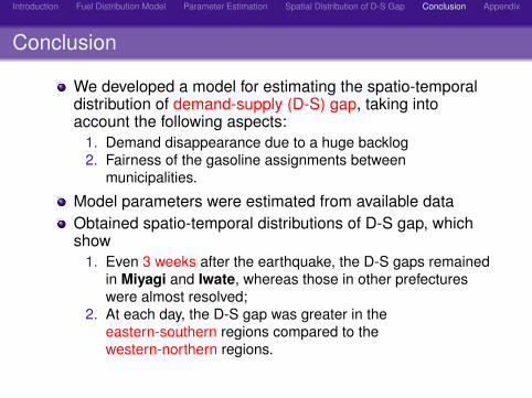
Conclusion
We developed a model for estimating the spatio-temporaldistribution of demand-supply (D-S) gap, taking intoaccount the following aspects:
1. Demand disappearance due to a huge backlog2. Fairness of the gasoline assignments between
municipalities.
Model parameters were estimated from available dataObtained spatio-temporal distributions of D-S gap, whichshow
1. Even 3 weeks after the earthquake, the D-S gaps remainedin Miyagi and Iwate, whereas those in other prefectureswere almost resolved;
2. At each day, the D-S gap was greater in theeastern-southern regions compared to thewestern-northern regions.
Introduction Fuel Distribution Model Parameter Estimation Spatial Distribution of D-S Gap Conclusion Appendix
Outline
1 Introduction
2 Fuel Distribution Model
3 Parameter Estimation
4 Spatial Distribution of D-S Gap
5 Conclusion
6 Appendix
Introduction Fuel Distribution Model Parameter Estimation Spatial Distribution of D-S Gap Conclusion Appendix
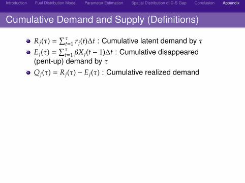
Cumulative Demand and Supply (Definitions)
R j(τ) =∑τ
t=1 r j(t)∆t : Cumulative latent demand by τE j(τ) =
∑τt=1 βX j(t − 1)∆t : Cumulative disappeared
(pent-up) demand by τQ j(τ) = R j(τ) − E j(τ) : Cumulative realized demand
Introduction Fuel Distribution Model Parameter Estimation Spatial Distribution of D-S Gap Conclusion Appendix
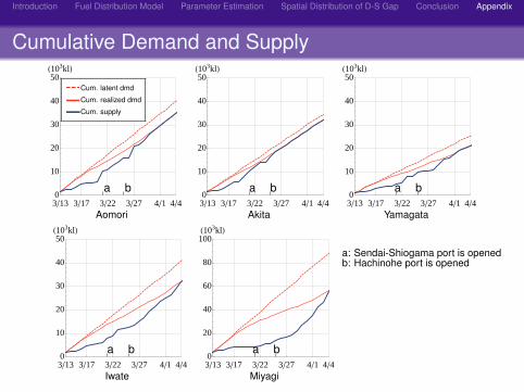
Cumulative Demand and Supply
3�13 3�17 3�22 3�27 4�1 4�40
10
20
30
40
50H103klL
Aomori
Cum. latent dmd
Cum. realized dmd
Cum. supply
3�13 3�17 3�22 3�27 4�1 4�40
10
20
30
40
50H103klL
Akita3�13 3�17 3�22 3�27 4�1 4�40
10
20
30
40
50H103klL
Yamagata
a ba ba b
3�13 3�17 3�22 3�27 4�1 4�40
10
20
30
40
50H103klL
Iwate3�13 3�17 3�22 3�27 4�1 4�40
20
40
60
80
100H103klL
Miyagi
a ba b
a: Sendai-Shiogama port is openedb: Hachinohe port is opened