Spatial variation in landscape-level CO 2 and CH 4 fluxes from arctic coastal tundra: influence from vegetation, wetness, and the thaw lake cycle

Spatial variation in landscape-level CO2 and CH4 fluxesfrom arctic coastal tundra: influence from vegetation,wetness, and the thaw lake cycleCOVE S . S TURTEVANT and WALTER C. OECHEL

Global Change Research Group, Department of Biology, San Diego State University, San Diego, CA, USA

Abstract

Regional quantification of arctic CO2 and CH4 fluxes remains difficult due to high landscape heterogeneity

coupled with a sparse measurement network. Most of the arctic coastal tundra near Barrow, Alaska is part of the

thaw lake cycle, which includes current thaw lakes and a 5500-year chronosequence of vegetated thaw lake basins.

However, spatial variability in carbon fluxes from these features remains grossly understudied. Here, we present

an analysis of whole-ecosystem CO2 and CH4 fluxes from 20 thaw lake cycle features during the 2011 growing

season. We found that the thaw lake cycle was largely responsible for spatial variation in CO2 flux, mostly due to

its control on gross primary productivity (GPP). Current lakes were significant CO2 sources that varied little. Veg-

etated basins showed declining GPP and CO2 sink with age (R2 = 67% and 57%, respectively). CH4 fluxes mea-

sured from a subset of 12 vegetated basins showed no relationship with age or CO2 flux components. Instead,

higher CH4 fluxes were related to greater landscape wetness (R2 = 57%) and thaw depth (additional R2 = 28%).

Spatial variation in CO2 and CH4 fluxes had good satellite remote sensing indicators, and we estimated the region

to be a small CO2 sink of �4.9 � 2.4 (SE) g C m�2 between 11 June and 25 August, which was countered by a

CH4 source of 2.1 � 0.2 (SE) g C m�2. Results from our scaling exercise showed that developing or validating

regional estimates based on single tower sites can result in significant bias, on average by a factor 4 for CO2 flux

and 30% for CH4 flux. Although our results are specific to the Arctic Coastal Plain of Alaska, the degree of land-

scape-scale variability, large-scale controls on carbon exchange, and implications for regional estimation seen here

likely have wide relevance to other arctic landscapes.

Keywords: Alaska, carbon dioxide, eddy covariance, methane, normalized difference red edge index, normalized difference

vegetation index, Tasseled Cap Transformation, upscaling

Received 24 January 2013; revised version received 27 April 2013 and accepted 29 April 2013

Introduction

The Arctic is rapidly changing. Atmospheric warming

in arctic regions has occurred at nearly double the glo-

bal rate (IPCC, 2007), thereby warming permafrost tem-

peratures (Shiklomanov et al., 2010), altering vegetation

communities (Sturm et al., 2001), and changing the

hydrological processes of many ecosystems (Hinzman

et al., 2005). Northern permafrost soils are estimated to

contain 1672 Pg of carbon, enough to more than double

the amount currently in the atmosphere (Zimov et al.,

2006; Tarnocai et al., 2009). The uncertain fate of this

large soil carbon pool necessitates accurate regional car-

bon source/sink estimation to track changes in the arc-

tic carbon balance and forecast future emissions.

However, developing regional estimates for the Arctic

are hampered by highly complex and heterogeneous

landscapes (McGuire et al., 2012).

High spatial variability in arctic land-atmosphere car-

bon exchange is due to the presence of impermeable

permafrost below a shallow summer thaw layer. This

results in water tables very close to the surface, and

therefore small variations in surface elevation (microto-

pography) lead to large differences in soil characteris-

tics, moisture, and vegetation over short spatial scales

(Brown et al., 1980). As these are some of the major fac-

tors controlling productivity and decomposition, the

variability in CO2 and CH4 fluxes at the ecosystem scale

or smaller can be similar to that over large latitudinal

and longitudinal transects (e.g., Morrissey & Living-

ston, 1992; Soegaard et al., 2000; McFadden et al., 2003).

Although the high spatial variability in arctic CO2

and CH4 flux rates is well known, few studies (espe-

cially for CH4) have measured and attributed this vari-

ability at the whole-ecosystem (eddy covariance tower)

level needed for improving regional estimates (but see

McFadden et al., 2003; Parmentier et al., 2011; Vourlitis

et al., 2003; Williams et al., 2000; Zona et al., 2010; Zulu-

eta et al., 2011). Therefore, validation of arctic regionalCorrespondence: C. S. Sturtevant, tel. + 303 489-8763,

fax + 619 594-7831, e-mail: [email protected]

© 2013 John Wiley & Sons Ltd 2853

Global Change Biology (2013) 19, 2853–2866, doi: 10.1111/gcb.12247

flux models often relies on a very sparse tower network

(e.g., Kimball et al., 2009) containing almost no informa-

tion about within-region variability.

On the Arctic Coastal Plain of Alaska near Barrow,

where this study is focused, the predominant landscape

variability consists of current and former thaw lakes.

Current lakes cover about 22% of the surface (Hinkel

et al., 2003). Another 50% is attributed to vegetated

thaw lake basins (VTLBs), which are previous thaw

lakes that drained at some point over that last ~5500years (Hinkel et al., 2003). The remaining 28% is

‘matrix’ tundra between the lakes and VTLBs. Thaw

lakes form via thermokarst processes (Cabot, 1947; Car-

son, 1968) and are shallow; 77% have depths <2.2 m

(Jeffries et al., 1996). Partial or total lake drainage can

occur at any time (Cabot, 1947; Carson, 1968). After

drainage, a slow process of ecosystem development

occurs over thousands of years until another lake

forms, often overlapping other VTLBs and restarting

the cycle (Billings & Peterson, 1980; Hinkel et al., 2003).

Although lakes and VTLBs cover 72% of the surface

and the ecological characteristics of VTLBs have been

well documented, landscape variability in CO2 and

CH4 fluxes arising from these features are not well

characterized. Kling et al.’s (1992) study of CO2 and

CH4 fluxes from lakes and rivers in Arctic Alaska sug-

gested that aquatic sources may reduce the regional

carbon sink by 20–50%. Despite this potentially large

importance, carbon flux estimates from thaw lakes on

the Arctic Coastal Plain of Alaska are few in number

and remain severely underrepresented in regional esti-

mation (for example, in McGuire et al., 2012). On the

terrestrial side, most CO2 flux studies in this region

have either focused on matrix tundra (e.g., Vourlitis &

Oechel, 1997; Kwon et al., 2006) or microform-level var-

iation (e.g., Oechel et al., 1995; Olivas et al., 2011). Only

two previous studies have addressed variability in CO2

flux along parts of the VTLB chronosequence (Zona

et al., 2010; Zulueta et al., 2011), but neither have

included variability from lakes or CH4 flux measure-

ments. Both these studies indicated that productivity

generally declines with age in the VTLBs, but much

uncertainty remains as to the influence of these features

on the net regional growing season CO2 balance. A few

VTLBs have been explicitly included in CH4 flux stud-

ies from this area (Zona et al., 2009; von Fischer et al.,

2010; Sturtevant et al., 2012), showing agreement with

the ample literature indicating soil moisture as a strong

driver of spatial variability (Morrissey & Livingston,

1992; Vourlitis et al., 1993; Christensen et al., 1995).

However, no studies have addressed the contribution

from the ecosystem development along the VTLB

chronosequence. Therefore, our objectives were to (i)

quantitatively determine how thaw lake cycle features

contribute to landscape-scale variability in net growing

season CO2 and CH4 fluxes; and (ii) determine whether

this knowledge can improve regional estimates. This

study represents one of very few arctic studies examin-

ing region-scale variability in whole-ecosystem CO2

flux and to our knowledge is the first of this breadth for

whole-ecosystem CH4 flux. Although the results pre-

sented here are specific to the Arctic Coastal Plain of

Alaska, the variability in carbon fluxes, large-scale con-

trols on carbon exchange, and implications for regional

scaling likely have wide relevance to other arctic land-

scapes.

Materials and methods

Site description

The wet meadow tundra near Barrow, Alaska lies within the

continuous permafrost zone, with maximum soil thaw reach-

ing 30–90 cm (Bockheim et al., 1999). Vegetation is dominated

by graminoids (incl. Arctophila fulva, Dupontia fisheri, Eriopho-

rum spp., Carex aquatilis), mosses (incl. Sphagnum, Dicranum

elongatum), lichens, and a few prostrate dwarf shrubs (Salix

spp., Cassiope tetragona) (Billings & Peterson, 1980; Hinkel et al.,

2003). The growing season extends from early June to late

August, with long-term (1971–2000) mean air temperature and

precipitation of 3.3 °C (�1.0 SD) and 56.5 mm (�26.8 SD),

respectively. The growing season of 2011 (the year of this

study) was warmer and slightly wetter than the long term

average (4.3 °C and 64.6 mm, respectively).

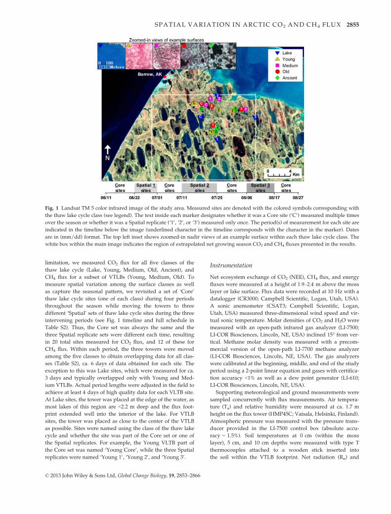
Previous work by Hinkel et al. (2003) classified the Barrow

area into five classes of the thaw lake cycle plus the remainder

of matrix tundra. We used this classification along with acces-

sibility by road or trail to identify sites for this study (Fig. 1;

Table S1). Thaw lake cycle classes include current lakes (Lake)

and four age classes of the ca. 5500 year VTLB chronose-

quence of ecosystem development after drainage (Young:

0–50 years, Medium: 50–300 years, Old: 300–2000 years, and

Ancient: 2000–5500 years.). Young, Medium, and Ancient

VTLBs are fewer in number, representing 4%, 9.2%, and 6.6%

of the land surface, respectively, while Old basins cover 30.4%

of the surface (Hinkel et al., 2003). Briefly, major VTLB

changes through time include: (i) general surface heave from

accumulation of ice and organic matter; (ii) increasing micro-

topography, polygon patterned ground and ponding (Fig. 1

inset) due to the expansion of ice wedges (which eventually

leads to the formation of a new lake); and (iii) a succession of

vegetation from fast growing pioneer species to longer lived,

low-vigor assemblages (Billings & Peterson, 1980; Hinkel et al.,

2003).

Study design

We used three portable eddy covariance towers deployed on

the tundra between 11 June and 27 August of 2011, all

equipped to measure CO2 flux and two of them equipped

to measure CH4 flux. As a result of the CH4 instrument

© 2013 John Wiley & Sons Ltd, Global Change Biology, 19, 2853–2866

2854 C. S . STURTEVANT & W. C. OECHEL

limitation, we measured CO2 flux for all five classes of the

thaw lake cycle (Lake, Young, Medium, Old, Ancient), and

CH4 flux for a subset of VTLBs (Young, Medium, Old). To

measure spatial variation among the surface classes as well

as capture the seasonal pattern, we revisited a set of ‘Core’

thaw lake cycle sites (one of each class) during four periods

throughout the season while moving the towers to three

different ‘Spatial’ sets of thaw lake cycle sites during the three

intervening periods (see Fig. 1 timeline and full schedule in

Table S2). Thus, the Core set was always the same and the

three Spatial replicate sets were different each time, resulting

in 20 total sites measured for CO2 flux, and 12 of these for

CH4 flux. Within each period, the three towers were moved

among the five classes to obtain overlapping data for all clas-

ses (Table S2), ca. 6 days of data obtained for each site. The

exception to this was Lake sites, which were measured for ca.

3 days and typically overlapped only with Young and Med-

ium VTLBs. Actual period lengths were adjusted in the field to

achieve at least 4 days of high quality data for each VLTB site.

At Lake sites, the tower was placed at the edge of the water, as

most lakes of this region are <2.2 m deep and the flux foot-

print extended well into the interior of the lake. For VTLB

sites, the tower was placed as close to the center of the VTLB

as possible. Sites were named using the class of the thaw lake

cycle and whether the site was part of the Core set or one of

the Spatial replicates. For example, the Young VLTB part of

the Core set was named ‘Young Core’, while the three Spatial

replicates were named ‘Young 1’, ‘Young 2’, and ‘Young 3’.

Instrumentation

Net ecosystem exchange of CO2 (NEE), CH4 flux, and energy

fluxes were measured at a height of 1.9–2.4 m above the moss

layer or lake surface. Flux data were recorded at 10 Hz with a

datalogger (CR3000; Campbell Scientific, Logan, Utah, USA).

A sonic anemometer (CSAT3; Campbell Scientific, Logan,

Utah, USA) measured three-dimensional wind speed and vir-

tual sonic temperature. Molar densities of CO2 and H2O were

measured with an open-path infrared gas analyzer (LI-7500;

LI-COR Biosciences, Lincoln, NE, USA) inclined 15° from ver-

tical. Methane molar density was measured with a precom-

mercial version of the open-path LI-7700 methane analyzer

(LI-COR Biosciences, Lincoln, NE, USA). The gas analyzers

were calibrated at the beginning, middle, and end of the study

period using a 2-point linear equation and gases with certifica-

tion accuracy <1% as well as a dew point generator (LI-610;

LI-COR Biosciences, Lincoln, NE, USA).

Supporting meteorological and ground measurements were

sampled concurrently with flux measurements. Air tempera-

ture (Ta) and relative humidity were measured at ca. 1.7 m

height on the flux tower (HMP45C; Vaisala, Helsinki, Finland).

Atmospheric pressure was measured with the pressure trans-

ducer provided in the LI-7500 control box (absolute accu-

racy = 1.5%). Soil temperatures at 0 cm (within the moss

layer), 5 cm, and 10 cm depths were measured with type T

thermocouples attached to a wooden stick inserted into

the soil within the VTLB footprint. Net radiation (Rn) and

Fig. 1 Landsat TM 5 color infrared image of the study area. Measured sites are denoted with the colored symbols corresponding with

the thaw lake cycle class (see legend). The text inside each marker designates whether it was a Core site (‘C’) measured multiple times

over the season or whether it was a Spatial replicate (‘1’, ‘2’, or ‘3’) measured only once. The period(s) of measurement for each site are

indicated in the timeline below the image (underlined character in the timeline corresponds with the character in the marker). Dates

are in (mm/dd) format. The top left inset shows zoomed-in nadir views of an example surface within each thaw lake cycle class. The

white box within the main image indicates the region of extrapolated net growing season CO2 and CH4 fluxes presented in the results.


SPATIAL VARIATION IN ARCTIC CO2 AND CH4 FLUX 2855

photosynthetically active radiation (PAR) were measured on

a ca. 1 m high tripod adjacent to the tower with a net radiom-

eter (NR-Lite, Kipp, & Zonen, Delft, The Netherlands) and

quantum sensor (LI-190; LI-COR Biosciences, Lincoln, NE,

USA), respectively. Ground heat flux was averaged over 4–5

ground heat flux plates (HFT3; Campbell Scientific, Logan,

Utah, USA) buried at 2 cm depth within the tower footprint.

We also took measurements of soil temperature, net radiation,

and ground heat flux at Lake sites, placing the sensors just

inside the lake edge. However, we found that meteorological

measurements on the tower were more useful in explaining

the data, likely because the lake edge was unrepresentative.

Therefore, these measurements are not presented.

Volumetric soil moisture in the top 7 cm of soil (FieldScout

TDR 300, Spectrum, Inc., Plainfield, IL, USA) and thaw depth

(graduated rod) were sampled by hand every 10 m along two

to three 100 m transects within the footprint of the VTLBs each

time a tower was brought to or removed from a site. Volumet-

ric soil moisture measurements were converted to ‘landscape

wetness’ by calculating the percent of the field measurements

at or above saturation. This soil moisture metric is presented

because it was the most informative in analyses, providing a

more standardized metric of aerobic vs. anaerobic soil status

of the site. Daily thaw depth and landscape wetness were

obtained by linear interpolation between sample dates.

Flux processing

All computational procedures were coded in MATLAB

v. 7.12.0 (Mathworks, Natick, Massachusetts, USA). Half-

hourly flux calculations were made using the eddy covariance

method (Baldocchi et al., 1988). Raw 10 Hz data were despi-

ked (>6 standard deviations from the 1-min running mean)

and filtered for periods clearly demonstrating error. The sonic

anemometer coordinate frame was double rotated to align

with the mean wind streamline and signals from separate sen-

sors were lag-corrected. Corrections were applied for simulta-

neous sensible and latent heat fluxes (Webb et al., 1980;

McDermitt et al., 2010), high frequency spectral loss (Moore,

1986), and the LI-7500 self-heating correction (Burba et al.,

2008) (Method 4 and linear regression therein). Computed

fluxes indicating nonstationarity (Foken et al., 2004), low tur-

bulence conditions (friction velocity <0.1 m s�1), and footprint

outside the feature of interest were rejected. Quality-

controlled fluxes showed cospectra similar to Kaimal et al.

(1972). Energy budget closure averaged 81% for VTLB classes,

which is just above the FLUXNET average (79%) (Wilson et al.,

2002), and there were no substantial differences among

classes. Energy closure for Lake sites was not evaluated due to

the large unknown storage term. A footprint model (Hsieh

et al., 2000) indicated that under most observed conditions

80% of measured fluxes were attributed to the first 150 m and

300 m upwind from the tower for VTLBs and Lake sites,

respectively.

During each period, daily averages of NEE for VTLB sites

were obtained by gap-filling missing half-hourly measure-

ments using a semi-empirical light and temperature response

model (Falge et al., 2001). Days were gap-filled only if the

quality-controlled data for that day ensured a good fit for the

model. No gap-filling was performed for NEE at Lake sites or

CH4 flux at any site due to small observed diurnal patterns. In

these cases, daily averages were calculated with available

measurements as long as at least 4 h of quality-controlled

NEE or CH4 flux was present for the day. The number of daily

averages used for final analysis by site and period, as well as

the percentage of quality-controlled (nongap-filled) data cov-

erage for those days are given in Table S3.

The measured daily average NEE for VTLB sites was then

partitioned into gross primary productivity (GPP) and ecosys-

tem respiration (ER) via the equation:

NEE ¼ GPPþ ER

Positive values indicate sources to the atmosphere. ER for

each day was measured as the NEE at zero light, either

directly observed (at night) or estimated from the y-intercept

of each day’s PAR-NEE relationship with a linear equation for

PAR <300 lmol quanta m�2 s�1 as long as at least 6 points

were available and P < 0.05.

Modeling and analysis methods

Seasonal modeling. To compute cumulative seasonal fluxes

and present baselines from which to evaluate spatial variation,

we modeled the seasonal trends of daily CO2 and CH4 fluxes

from the Core sites. The purpose of this modeling was not to

strictly test physiological models published for other arctic

studies, but to provide the best possible extrapolation of Core

site fluxes during Spatial periods. Seasonal models for Lake

Core NEE as well as CH4 flux from all Core sites were mod-

eled solely according to correlations in the data and are pre-

sented in the Results. Seasonal NEE models for the Core

VTLBs were modified versions of those in Loranty et al.

(2011). Descriptions of the NEE models as well as coefficients

and performance plots are presented in Section 3 of the Sup-

porting Information. Monte Carlo simulation was performed

to determine statistical uncertainty on cumulative fluxes com-

puted from the seasonal models. Each modeled daily flux was

assigned a normally distributed random error with mean of 0

and standard deviation equal to the root mean square error

(RMSE) of the model. This procure was performed 1000 times

and the standard deviation of the resultant cumulative fluxes

computed.

Normalization. Since only three sites could be measured at

any one time, comparing fluxes and environmental measure-

ments among sites was sometimes confounded by daily varia-

tion and seasonal trends. Therefore, for measurements of thaw

depth, GPP, ER, and NEE we normalized Spatial site measure-

ments to baselines derived from interpolated or modeled

values from the Core sites to remove temporal variation and

isolate spatial differences. The mean thaw depth for each site

and period was converted to a percent difference from the

average Core VTLB thaw depth (interpolated) for the corre-

sponding days. Normalization of CO2 flux components for the

VTLB sites was done by calculating the relative magnitude of

the average daily flux for each site in relation to the minimum



and maximum modeled Core VTLB fluxes for the correspond-

ing days via the equation:

Fnorm ¼ Fave � FCmin

FCmax � FCmin

F indicates the flux (NEE, GPP, or ER). Fnorm and Fave are the

normalized and nonnormalized average daily flux, respec-

tively, for a given site and period. FCmin and FCmax are the

minimum and maximum average modeled Core VTLB fluxes,

respectively, for the same days included in Fave. To retain gen-

eral sign conventions, GPPnorm and NEEnorm were subtracted

from 1 and the result multiplied by �1. A normalization

example using the data is given in Section 4 of the Supporting

Information.

Spatial analysis. After any normalization procedures, daily

measurements were averaged for each site and period (‘per-

iod-average’) for final analysis of spatial variation. The middle

two Core periods were averaged to provide one period-aver-

age value for each Core site since these two periods were clos-

est to the time frame of the Spatial measurements and showed

the best separability among sites. To analyze differences in

fluxes and environmental variables among sites, we used ANO-

VA and multiple regression. Post hoc pairwise comparisons for

ANOVA models were performed using Tukey’s Honestly Signifi-

cant Difference Criterion to control the Type I error rate (0.05).

To estimate the range of cumulative fluxes from all VTLB

sites, we substituted the normalized NEE values or period-

averaged CH4 values with cumulative season totals using the

relationships observed for the Core sites (shown in Section 5

of the Supporting Information). Cumulative season totals for

each of the Lake sites was estimated using the percent differ-

ence of each site from the Lake Core seasonal model. We used

the Monte Carlo procedure outlined above to determine the

statistical uncertainty on cumulative fluxes of the Spatial repli-

cate sites estimated via the relationship between normalized

or mid-season averages and cumulative fluxes for the Core

sites. In this case, the values in the regression were varied

within their individual uncertainties.

Regional scaling

We related our observations to established remote sensing

metrics acquired from satellite imagery and scaled our results

to a 170 km2 region surrounding our sites (white box in

Fig. 1). We used a high resolution (2 m) Worldview 2 image

(Basic LV1B product; Digital Globe Inc., Longmont, CO, USA)

from 21 July 2010 and a moderate resolution (30 m) Landsat

TM 5 image (Level 1T product) from 6 August 2011. Although

the Worldview 2 image was from 2010, we reasoned that spa-

tial differences among sites would remain similar between the

2010 and 2011 growing seasons, as the climatic conditions in

2010 and 2011 were not drastically different and ecosystem

change in this landscape occurs over much longer time scales.

We computed three physically based remote sensing met-

rics, including the Normalized Difference Vegetation Index

(‘NDVI’; Rouse et al., 1973), the Normalized Difference Red

Edge index (‘NDRE’; Barnes et al., 2000), and the Landsat TM

5 Tasseled Cap Transformation Wetness index (‘TCTw’; Crist

& Cicone, 1984). Higher NDVI values indicate more green,

healthy vegetation, and NVDI has shown good correlation

with arctic GPP and NEE (McMichael et al., 1999; Vourlitis

et al., 2000; Zulueta et al., 2011). NDRE is a close relative of

NDVI demonstrated to show enhanced sensitivity to plant

health (Tilling et al., 2007; Eitel et al., 2011). TCTw provides a

metric for surface water status, higher values indicating

greater surface moisture (Adams & Gillespie, 2006). Due to

sensor-specific bands, NDVI was calculated from both images,

NDRE from the WoldView 2 image only, and TCTw from the

Landsat TM 5 image only.

All image processing was performed in ENVI 5.0 (Exelis,

Inc., McLean, Virginia, USA). The Beaufort Sea, clouds, and

urban areas were masked out (3% of the WorldView 2 image,

7.8% of the Landsat TM 5 image). Remote sensing metrics

were computed from the digital numbers of the imagery with

no further radiometric or geometric corrections. Mean values

for each VTLB site were computed for the pixels within the

80% cumulative flux footprint. The borders of lakes and

VTLBs were digitized by hand. Lakes, VTLBs, and matrix tun-

dra accounted for 16%, 51%, and 34% of the 170 km2 region,

respectively.

We again used the Monte Carlo procedure outlined above

to determine the statistical uncertainty on regional fluxes com-

puted using regressions between remotely sensed indices and

observed fluxes.

Results

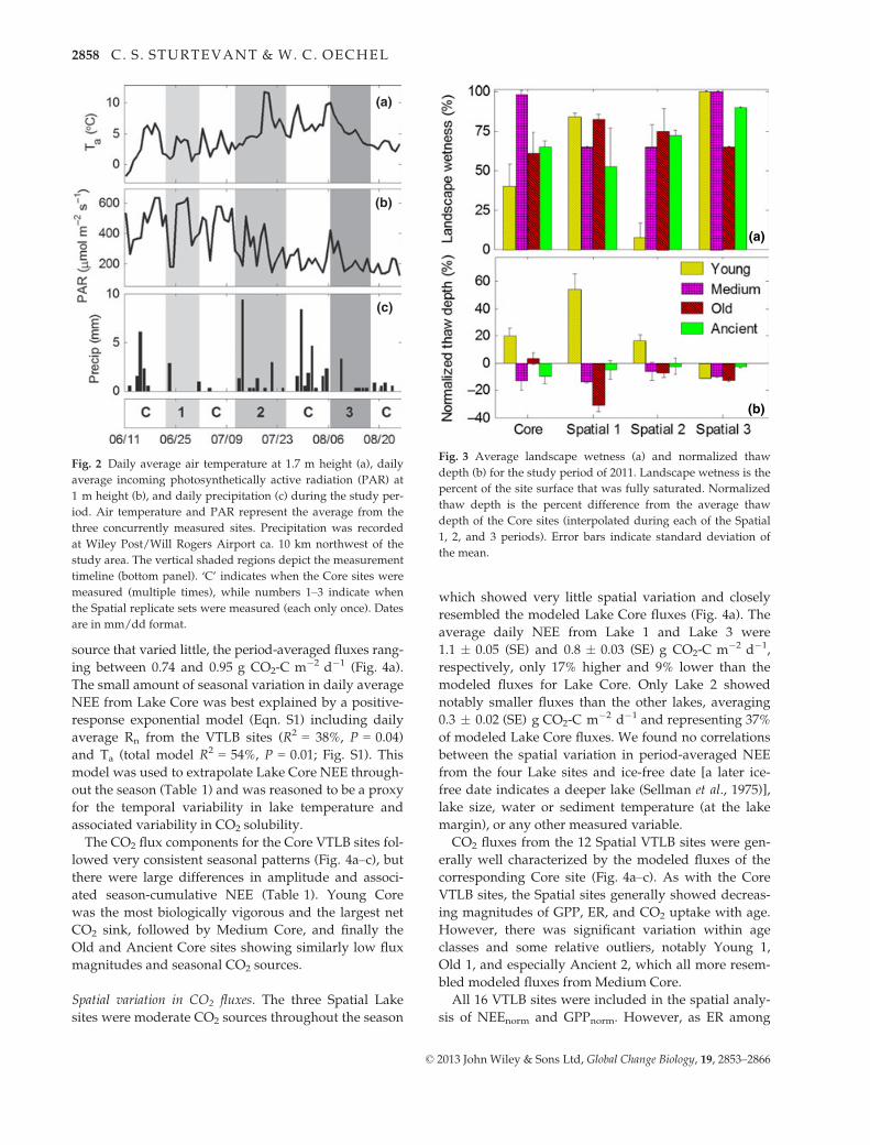
Environmental and site conditions

During the study period, air temperature showed a

broad peak in late July and early August (Fig. 2a), PAR

generally declined (Fig. 2b), and liquid precipitation

was intermittent (Fig. 2c). Ice-free dates of the Lake

measurement sites were estimated from Landsat imag-

ery: Lake Core on 21 June, Lake 3 on 27 June, Lake 1 on

5 July, and Lake 2 between 6 and 12 July.

There was no consistent seasonal pattern in land-

scape wetness observed from the Core VTLBs. Includ-

ing the Spatial sites, period-average landscape wetness

ranged from near dry to completely flooded (Fig. 3a),

but landscape wetness was not associated with VTLB

age class (P = 0.54). In general, Young VTLBs exhibited

relatively higher thaw depth than the other age classes,

which showed no consistent differences (Fig. 3b;

P = 0.04). Other than thaw depth, no measured envi-

ronmental variables showed relative differences associ-

ated with VTLB age class (including soil temperature,

ground heat flux, and net radiation).

CO2 fluxes

Seasonal variation in CO2 fluxes (Core sites). During the

growing season, Lake Core was a substantial CO2



source that varied little, the period-averaged fluxes rang-

ing between 0.74 and 0.95 g CO2-C m�2 d�1 (Fig. 4a).

The small amount of seasonal variation in daily average

NEE from Lake Core was best explained by a positive-

response exponential model (Eqn. S1) including daily

average Rn from the VTLB sites (R2 = 38%, P = 0.04)

and Ta (total model R2 = 54%, P = 0.01; Fig. S1). This

model was used to extrapolate Lake Core NEE through-

out the season (Table 1) and was reasoned to be a proxy

for the temporal variability in lake temperature and

associated variability in CO2 solubility.

The CO2 flux components for the Core VTLB sites fol-

lowed very consistent seasonal patterns (Fig. 4a–c), butthere were large differences in amplitude and associ-

ated season-cumulative NEE (Table 1). Young Core

was the most biologically vigorous and the largest net

CO2 sink, followed by Medium Core, and finally the

Old and Ancient Core sites showing similarly low flux

magnitudes and seasonal CO2 sources.

Spatial variation in CO2 fluxes. The three Spatial Lake

sites were moderate CO2 sources throughout the season

which showed very little spatial variation and closely

resembled the modeled Lake Core fluxes (Fig. 4a). The

average daily NEE from Lake 1 and Lake 3 were

1.1 � 0.05 (SE) and 0.8 � 0.03 (SE) g CO2-C m�2 d�1,

respectively, only 17% higher and 9% lower than the

modeled fluxes for Lake Core. Only Lake 2 showed

notably smaller fluxes than the other lakes, averaging

0.3 � 0.02 (SE) g CO2-C m�2 d�1 and representing 37%

of modeled Lake Core fluxes. We found no correlations

between the spatial variation in period-averaged NEE

from the four Lake sites and ice-free date [a later ice-

free date indicates a deeper lake (Sellman et al., 1975)],

lake size, water or sediment temperature (at the lake

margin), or any other measured variable.

CO2 fluxes from the 12 Spatial VTLB sites were gen-

erally well characterized by the modeled fluxes of the

corresponding Core site (Fig. 4a–c). As with the Core

VTLB sites, the Spatial sites generally showed decreas-

ing magnitudes of GPP, ER, and CO2 uptake with age.

However, there was significant variation within age

classes and some relative outliers, notably Young 1,

Old 1, and especially Ancient 2, which all more resem-

bled modeled fluxes from Medium Core.

All 16 VTLB sites were included in the spatial analy-

sis of NEEnorm and GPPnorm. However, as ER among

(a)

(b)

(c)

Fig. 2 Daily average air temperature at 1.7 m height (a), daily

average incoming photosynthetically active radiation (PAR) at

1 m height (b), and daily precipitation (c) during the study per-

iod. Air temperature and PAR represent the average from the

three concurrently measured sites. Precipitation was recorded

at Wiley Post/Will Rogers Airport ca. 10 km northwest of the

study area. The vertical shaded regions depict the measurement

timeline (bottom panel). ‘C’ indicates when the Core sites were

measured (multiple times), while numbers 1–3 indicate when

the Spatial replicate sets were measured (each only once). Dates

are in mm/dd format.

(a)

(b)

Fig. 3 Average landscape wetness (a) and normalized thaw

depth (b) for the study period of 2011. Landscape wetness is the

percent of the site surface that was fully saturated. Normalized

thaw depth is the percent difference from the average thaw

depth of the Core sites (interpolated during each of the Spatial

1, 2, and 3 periods). Error bars indicate standard deviation of

the mean.



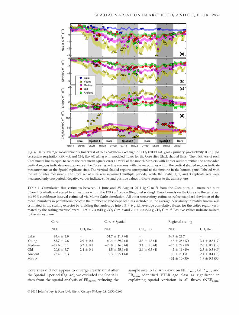
Core sites did not appear to diverge clearly until after

the Spatial 1 period (Fig. 4c), we excluded the Spatial 1

sites from the spatial analysis of ERnorm, reducing the

sample size to 12. An ANOVA on NEEnorm, GPPnorm, and

ERnorm identified VTLB age class as significant in

explaining spatial variation in all fluxes (NEEnorm:

(a)

(b)

(c)

(d)

Fig. 4 Daily average measurements (markers) of net ecosystem exchange of CO2 (NEE) (a), gross primary productivity (GPP) (b),

ecosystem respiration (ER) (c), and CH4 flux (d) along with modeled fluxes for the Core sites (thick shaded lines). The thickness of each

Core model line is equal to twice the root mean square error (RMSE) of the model. Markers with lighter outlines within the nonshaded

vertical regions indicate measurements at the Core sites, while markers with darker outlines within the vertical shaded regions indicate

measurements at the Spatial replicate sites. The vertical-shaded regions correspond to the timeline in the bottom panel (labeled with

the set of sites measured). The Core set of sites was measured multiple periods, while the Spatial 1, 2, and 3 replicate sets were

measured only one period. Negative values indicate sinks and positive values indicate sources to the atmosphere.

Table 1 Cumulative flux estimates between 11 June and 25 August 2011 (g C m�2) from the Core sites, all measured sites

(Core + Spatial), and scaled to all features within the 170 km2 region (Regional scaling). Error bounds on the Core site fluxes reflect

the 99% confidence interval estimated via Monte Carlo simulation. All other uncertainty estimates reflect standard deviation of the

mean. Numbers in parenthesis indicate the number of landscape features included in the average. Variability in matrix tundra was

estimated in the scaling exercise by dividing the landscape into a 5 9 6 grid. Average cumulative fluxes for the entire region (esti-

mated by the scaling exercise) were �4.9 � 2.4 (SE) g CO2-C m�2 and 2.1 � 0.2 (SE) g CH4-C m�2. Positive values indicate sources

to the atmosphere

Core Core + Spatial Regional scaling

NEE CH4 flux NEE CH4 flux NEE CH4 flux

Lake 63.4 � 2.9 – 54.7 � 21.7 (4) – 54.7 � 21.7 –

Young �85.7 � 9.6 2.9 � 0.3 �60.4 � 39.7 (4) 3.3 � 1.5 (4) �46 � 28 (17) 3.1 � 0.8 (17)

Medium �17.6 � 5.1 3.3 � 0.1 �29.8 � 16.5 (4) 3.1 � 1.0 (4) �13 � 22 (19) 2.6 � 0.7 (19)

Old 20.8 � 3.7 2.4 � 0.1 4.5 � 25.9 (4) 2.9 � 0.5 (4) �2 � 11 (49) 2.3 � 0.5 (49)

Ancient 23.4 � 3.3 – 7.3 � 25.1 (4) – 10 � 7 (15) 2.1 � 0.4 (15)

Matrix – – – – �32 � 10 (30) 1.9 � 0.3 (30)



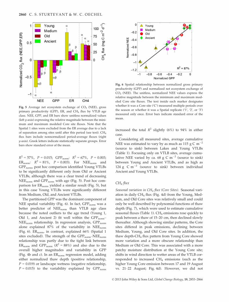
R2 = 57%, P = 0.015; GPPnorm: R2 = 67%, P = 0.003;

ERnorm: R2 = 81%, P = 0.003). For NEEnorm and

GPPnorm, post hoc comparison identified Young VTLBs

to be significantly different only from Old or Ancient

VTLBs, although there was a clear trend of decreasing

NEEnorm and GPPnorm with age (Fig. 5). Post hoc com-

parison for ERnorm yielded a similar result (Fig. 5), but

in this case Young VTLBs were significantly different

from Medium, Old, and Ancient VTLBs.

The partitioned GPP was the dominant component of

NEE spatial variability (Fig. 6). In fact, GPPnorm was a

better predictor of NEEnorm than VTLB age class

because the noted outliers to the age trend (Young 1,

Old 1, and Ancient 2) fit well within the GPPnorm–NEEnorm relationship. In regression analysis, GPPnorm

alone explained 87% of the variability in NEEnorm

(Fig. 6). ERnorm, in contrast, explained 66% (Spatial 1

sites excluded). The strength of the GPPnorm–NEEnorm

relationship was partly due to the tight link between

ERnorm and GPPnorm (R2 = 88%) and also due to the

overall higher magnitudes and variability in GPP

(Fig. 4b and c). In an ERnorm regression model, adding

either normalized thaw depth (positive relationship,

P = 0.019) or landscape wetness (negative relationship,

P = 0.015) to the variability explained by GPPnorm

increased the total R2 slightly (6%) to 94% in either

case.

Considering all measured sites, average cumulative

NEE was estimated to vary by as much as 115 g C m�2

(source to sink) between Lakes and Young VTLBs

(Table 1). Focusing only on VTLB sites, average cumu-

lative NEE varied by ca. 68 g C m�2 (source to sink)

between Young and Ancient VTLBs, and as high as

124 g C m�2 (source to sink) between individual

Ancient and Young VTLBs.

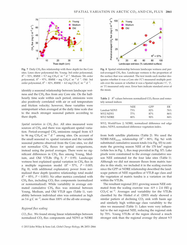
CH4 flux

Seasonal variation in CH4 flux (Core Sites). Seasonal vari-

ation in daily CH4 flux (Fig. 4d) from the Young, Med-

ium, and Old Core sites was relatively small and could

only be well described by polynomial functions of thaw

depth (Fig. 7), which were used to estimate cumulative

seasonal fluxes (Table 1). CH4 emissions rose quickly to

peak between a thaw of 15–20 cm, then declined slowly

thereafter. Although showing similar patterns, the Core

sites differed in peak emissions, declining between

Medium, Young, and Old Core sites. In addition, the

thaw depth-CH4 flux pattern from Young Core showed

more variation and a more obscure relationship than

Medium or Old Core. This was associated with a more

patchy moisture distribution at the Young Core site;

shifts in wind direction to wetter areas of the VTLB cor-

responded to increased CH4 emissions (such as the

higher Young Core emission between 17 and 19 August

vs. 21–22 August; Fig. 4d). However, we did not

Fig. 5 Average net ecosystem exchange of CO2 (NEE), gross

primary productivity (GPP), ER, and CH4 flux by VTLB age

class. NEE, GPP, and ER bars show unitless normalized values

(left y-axis) expressing the relative magnitude between the mini-

mum and maximum modeled Core site fluxes. Note that the

Spatial 1 sites were excluded from the ER average due to a lack

of separation among sites until after this period (see text). CH4

flux bars include nonnormalized period-average fluxes (right

y-axis). Greek letters indicate statistically separate groups. Error

bars show standard error of the mean.

Fig. 6 Spatial relationship between normalized gross primary

productivity (GPP) and normalized net ecosystem exchange of

CO2 (NEE). The unitless, normalized NEE values express the

relative magnitude between the minimum and maximum mod-

eled Core site fluxes. The text inside each marker designates

whether it was a Core site (‘C’) measured multiple periods over

the season or whether it was a Spatial replicate (‘1’, ‘2’, or ‘3’)

measured only once. Error bars indicate standard error of the

mean.



identify a seasonal relationship between landscape wet-

ness and the CH4 flux from any Core site. On the half-

hourly time scale within each period, emissions were

also positively correlated with air or soil temperature

and friction velocity; however, these variables were

unimportant when averaged at the daily time scale due

to the much stronger seasonal pattern according to

thaw depth.

Spatial variation in CH4 flux. All sites measured were

sources of CH4 and there was significant spatial varia-

tion. Period-averaged CH4 emissions ranged from 4.5

to 96 mg CH4-C m�2 d�1 among sites. On account of

the small seasonal vs. spatial variation and the variable

seasonal patterns observed from the Core sites, we did

not normalize CH4 fluxes for spatial comparisons,

instead using the period averages. There were no sig-

nificant differences in CH4 flux among Young, Med-

ium, and Old VTLBs (Fig. 5; P = 0.95). Landscape

wetness best explained spatial variation in CH4 flux in

a multiple regression model (R2 = 57%, P = 0.005;

Fig. 8), with additional explanatory power from nor-

malized thaw depth (positive relationship; total model

R2 = 85%, P < 0.001). No other metrics correlated with

CH4 flux, including CO2 flux components (normalized

or nonnormalized). While variability in average esti-

mated cumulative CH4 flux was minimal between

Young, Medium, and Old VTLB ages (Table 1), vari-

ability between individual sites was estimated as high

as 3.6 g C m�2, more than 100% of the all-site average.

Regional flux scaling

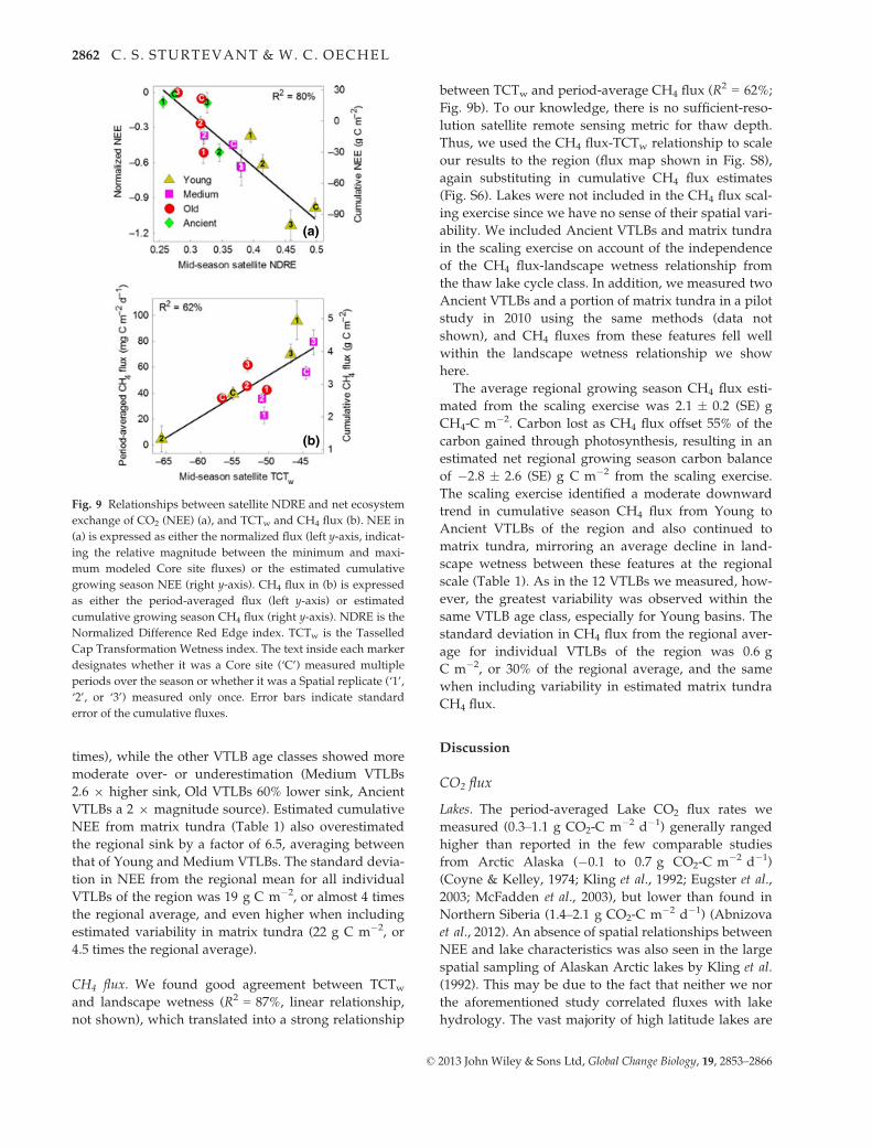
CO2 flux. We found strong linear relationships between

normalized CO2 flux components and NDVI or NDRE

from both satellite platforms (Table 2). We used the

NDRE-NEEnorm relationship (R2 = 80%; Fig. 9a) with

substituted cumulative season totals (via Fig. S5) to esti-

mate the growing season NEE of the 170 km2 region

(white box in Fig. 1, flux map provided in Fig. S7). Lake

pixels were constrained to the average cumulative sea-

son NEE estimated for the four lake sites (Table 1).

Although we did not measure fluxes from matrix tun-

dra in this study, we included it in the scaling exercise

since the GPP or NDRE relationship described the land-

scape pattern of NEE regardless of VTLB age class and

the vegetation of matrix tundra is a variation on that

within the VTLBs.

The resultant regional 2011 growing season NEE esti-

mated from the scaling exercise was -4.9 � 2.4 (SE) g

CO2-C m�2. Averages and variability for the VTLBs

classified by the Hinkel et al. (2003) study showed a

similar pattern of declining CO2 sink with basin age

and similarly high within-age class variability to the

sites we measured (Table 1). Lakes were very influen-

tial to the net regional NEE, reducing the regional sink

by 70%. Young VTLBs of the region showed a much

stronger sink than the regional average (by almost 9.5

Fig. 7 Daily CH4 flux relationship with thaw depth for the Core

sites. Lines show polynomial fits. Young: 3rd order polynomial,

R2 = 52%, RMSE = 9.7 mg CH4-C m�2 d�1. Medium: 5th order

polynomial, R2 = 97%, RMSE = mg CH4-C m�2 d�1. Old: 3rd

order polynomial, R2 = 82%, RMSE = 4.0 mg CH4-C m�2 d�1.

Fig. 8 Spatial relationship between landscape wetness and per-

iod-averaged CH4 flux. Landscape wetness is the proportion of

the surface that was saturated. The text inside each marker des-

ignates whether it was a Core site (‘C’) measured multiple peri-

ods over the season or whether it was a Spatial replicate (‘1’, ‘2’,

or ‘3’) measured only once. Error bars indicate standard error of

the mean.

Table 2 R2 values between normalized CO2 fluxes and remo-

tely sensed indices

NEE GPP ER

Landsat NDVI 73% 82% 76%

WV2 NDVI 77% 87% 86%

WV2 NDRE 80% 90% 84%

WV2, WorldView 2; NDRE, normalized difference red edge

index; NDVI, normalized difference vegetation index.



times), while the other VTLB age classes showed more

moderate over- or underestimation (Medium VTLBs

2.6 9 higher sink, Old VTLBs 60% lower sink, Ancient

VTLBs a 2 9 magnitude source). Estimated cumulative

NEE from matrix tundra (Table 1) also overestimated

the regional sink by a factor of 6.5, averaging between

that of Young and Medium VTLBs. The standard devia-

tion in NEE from the regional mean for all individual

VTLBs of the region was 19 g C m�2, or almost 4 times

the regional average, and even higher when including

estimated variability in matrix tundra (22 g C m�2, or

4.5 times the regional average).

CH4 flux. We found good agreement between TCTw

and landscape wetness (R2 = 87%, linear relationship,

not shown), which translated into a strong relationship

between TCTw and period-average CH4 flux (R2 = 62%;

Fig. 9b). To our knowledge, there is no sufficient-reso-

lution satellite remote sensing metric for thaw depth.

Thus, we used the CH4 flux-TCTw relationship to scale

our results to the region (flux map shown in Fig. S8),

again substituting in cumulative CH4 flux estimates

(Fig. S6). Lakes were not included in the CH4 flux scal-

ing exercise since we have no sense of their spatial vari-

ability. We included Ancient VTLBs and matrix tundra

in the scaling exercise on account of the independence

of the CH4 flux-landscape wetness relationship from

the thaw lake cycle class. In addition, we measured two

Ancient VTLBs and a portion of matrix tundra in a pilot

study in 2010 using the same methods (data not

shown), and CH4 fluxes from these features fell well

within the landscape wetness relationship we show

here.

The average regional growing season CH4 flux esti-

mated from the scaling exercise was 2.1 � 0.2 (SE) g

CH4-C m�2. Carbon lost as CH4 flux offset 55% of the

carbon gained through photosynthesis, resulting in an

estimated net regional growing season carbon balance

of �2.8 � 2.6 (SE) g C m�2 from the scaling exercise.

The scaling exercise identified a moderate downward

trend in cumulative season CH4 flux from Young to

Ancient VTLBs of the region and also continued to

matrix tundra, mirroring an average decline in land-

scape wetness between these features at the regional

scale (Table 1). As in the 12 VTLBs we measured, how-

ever, the greatest variability was observed within the

same VTLB age class, especially for Young basins. The

standard deviation in CH4 flux from the regional aver-

age for individual VTLBs of the region was 0.6 g

C m�2, or 30% of the regional average, and the same

when including variability in estimated matrix tundra

CH4 flux.

Discussion

CO2 flux

Lakes. The period-averaged Lake CO2 flux rates we

measured (0.3–1.1 g CO2-C m�2 d�1) generally ranged

higher than reported in the few comparable studies

from Arctic Alaska (�0.1 to 0.7 g CO2-C m�2 d�1)

(Coyne & Kelley, 1974; Kling et al., 1992; Eugster et al.,

2003; McFadden et al., 2003), but lower than found in

Northern Siberia (1.4–2.1 g CO2-C m�2 d�1) (Abnizova

et al., 2012). An absence of spatial relationships between

NEE and lake characteristics was also seen in the large

spatial sampling of Alaskan Arctic lakes by Kling et al.

(1992). This may be due to the fact that neither we nor

the aforementioned study correlated fluxes with lake

hydrology. The vast majority of high latitude lakes are

(a)

(b)

Fig. 9 Relationships between satellite NDRE and net ecosystem

exchange of CO2 (NEE) (a), and TCTw and CH4 flux (b). NEE in

(a) is expressed as either the normalized flux (left y-axis, indicat-

ing the relative magnitude between the minimum and maxi-

mum modeled Core site fluxes) or the estimated cumulative

growing season NEE (right y-axis). CH4 flux in (b) is expressed

as either the period-averaged flux (left y-axis) or estimated

cumulative growing season CH4 flux (right y-axis). NDRE is the

Normalized Difference Red Edge index. TCTw is the Tasselled

Cap Transformation Wetness index. The text inside each marker

designates whether it was a Core site (‘C’) measured multiple

periods over the season or whether it was a Spatial replicate (‘1’,

‘2’, or ‘3’) measured only once. Error bars indicate standard

error of the cumulative fluxes.



CO2 sources due to terrestrial carbon input from sur-

face runoff (Kling et al., 1992; Heikkinen et al., 2004;

Repo et al., 2007; Abnizova et al., 2012). Indeed, greater

lake flushing correlates with higher pCO2 (Sobek et al.,

2003; Tank et al., 2009). The lower emission from Lake 2

may have resulted from poor hydrological connectivity

with the landscape, as Lake 2 abuts the coast and does

not appear to be fed by any major surface flows.

VTLBs. The seasonal patterns and general magnitudes

of CO2 flux components we observed for the VTLB sites

were comparable to previous ecosystem-level studies in

arctic peatlands (e.g., Oechel et al., 1998a; Soegaard

et al., 2000; Vourlitis et al., 2000; Corradi et al., 2005;

Kwon et al., 2006; Loranty et al., 2011; Tagesson et al.,

2012). Our observations of declining productivity and

CO2 sink strength with VTLB age were also generally

consistent with the two previous regional flux studies

from these features (Zona et al., 2010; Zulueta et al.,

2011), although through the normalization and

increased sample size we show the trend to be much

clearer. Declining productivity with VTLB age is likely

a result of nutrients being locked up in slow decompos-

ing organic matter (Zona et al., 2010), as well as

increased ponding and associated strong CO2 source

(Coyne & Kelley, 1974; Abnizova et al., 2012). However,

there was also substantial variation within classes

observed in this and the two previous studies, exempli-

fied by the outliers we noted. However, aside from

Ancient 2 the CO2 fluxes from the outliers deviated by

only one age class, suggesting that other (unmeasured)

factors modify but generally do not replace the age

trend. As an example, the surprising productivity of

Ancient 2 might be caused by the drainage for Young 1

running directly through Ancient 2, possibly importing

nutrients and enhancing diffusion to roots via increased

soil water flow (Chapin et al., 1988; Oberbauer et al.,

1989; Rastetter et al., 2004).

It was surprising that large spatial variation in mois-

ture and thaw explained little spatial variation in CO2

flux components. Both these variables have a known

significant effect on decomposition rate in arctic soils

(e.g., Peterson et al., 1984; Oechel et al., 1998b; Olivas

et al., 2010) and greater wetness has been linked to

greater productivity in some studies (e.g., Oberbauer

et al., 1989; Sjogersten et al., 2006). We see two major

reasons for a lack of strong effect from either soil mois-

ture or thaw on spatial variation in NEE. First, the fac-

tors which influence ER (such as moisture and thaw)

can similarly affect GPP (Oberbauer et al., 2007; Olivas

et al., 2010). Second, the spatial variability in GPP was

very large, and since ER includes autotrophic respira-

tion to sustain plant biomass, variability in the auto-

trophic component of respiration (linked to GPP) likely

dominated the variability in ER. The strong relationship

we found between GPP and ER supports these link-

ages. Several other arctic studies have found that GPP

(or LAI as a proxy) controlled differences in NEE across

plant communities (Soegaard et al., 2000; McFadden

et al., 2003; Shaver et al., 2007; Lafleur et al., 2012). Thus,

the strong control of NEE variability by GPP is not

new, but we demonstrate that the ecosystem develop-

ment along the VTLB chronosequence largely drives

the spatial variability in GPP.

CH4 flux

The general flux rates, magnitude of seasonal variation,

and high spatial variability in CH4 emission we

observed from Young, Medium, and Old VTLBs were

consistent with previous arctic studies (e.g., Whalen &

Reeburgh, 1988; Vourlitis et al., 1993; Christensen et al.,

1995; Friborg et al., 2000; Sachs et al., 2008; Merbold

et al., 2009; von Fischer et al., 2010; Tagesson et al.,

2012). Surprising, however, was characterization of the

seasonal CH4 flux pattern only by thaw, which has been

found to limit emissions during the early season (e.g.,

Friborg et al., 2000; Tagesson et al., 2012) but to our

knowledge has not been explicitly linked to an early

peak and long decline. We suggest that the broad peak

in seasonal CH4 emission around 15–20 cm thaw could

reflect a lag in methanotrophy until higher soil methane

concentrations (Dedysh & Panikov, 1997; Segers, 1998;

Ambus & Petersen, 2005) or deeper thaw layers (Pani-

kov & Dedysh, 2000) were reached.

The strong control of spatial variability in CH4 flux

by landscape wetness and secondarily by relative thaw

is consistent with many smaller scale studies (e.g.,

Sebacher et al., 1986; Morrissey & Livingston, 1992;

Vourlitis et al., 1993; Christensen et al., 1995; Parmentier

et al., 2011). Water table position controls the volumes

of anaerobic and aerobic soil favorable for methane pro-

duction and oxidation, respectively (Bubier et al., 1993)

and thaw depth controls the total soil volume available

for decomposition. The most interesting aspect of this

result was the lack of relationship between CO2 and

CH4 fluxes as seen elsewhere (e.g., Whiting & Chanton,

1993; Tagesson et al., 2012), suggesting that even the

early stages of ecosystem development in this region

are not carbon limited.

Unfortunately, our limited resources prevented mea-

surement of spatial variation in Lake CH4 flux.

Although a few previous studies have found moder-

ately low lake CH4 emissions on the North Slope of

Alaska (Kling et al., 1992; Morrissey & Livingston,

1992), this is an important topic of future study, espe-

cially regarding the potential for large ebullitive CH4

emission (Walter et al., 2007).



Regional estimates

The individual sites we measured along with our

scaling exercise suggest that single long term tower

measurements typically used to validate regional

models (e.g., Kimball et al., 2009) can be substantially

biased. Not only did we observe strong variability in

NEE among the classes of the thaw lake cycle (from

source to sink and an order of magnitude) but also

substantial variability within these classes (about

equal to the magnitude of the average flux). In addi-

tion, the high CO2 source of lakes resulted in a

strong (70%) reduction in the regional average CO2

sink, and should certainly be accounted for in regio-

nal estimates. Although bias in regional CH4 flux

estimates from single tower sites would not generally

be tied to the age sequence of VTLBs, variability in

wetness and associated CH4 flux across the landscape

due to the presence of any VTLB was quite strong.

Thus, any one tower site, although integrating the

variability within that specific ecosystem, will likely

not be representative of the regional average flux,

easily off by a factor 4 for NEE and 30% for CH4 flux

as indicated by our scaling exercise.

We think the information on spatial variability we

present here can improve regional growing carbon

exchange estimation for Alaskan Arctic coastal tundra

and possible many other arctic regions. We suggest that

accurate CO2 and CH4 flux scaling can be accomplished

with a few well-placed tower sites and satellite remote

sensing proxies for productivity and landscape wet-

ness, respectively, to calibrate the type of scaling rela-

tionships observed here for each growing season (and

region). Although the ecosystem succession along the

VTLB chronosequence was the mechanism largely

behind spatial variation in GPP (and hence NEE), we

did not need it to scale to the region because GPP (and

its proxies of NDRE or NDVI) reflected not only the age

trend but also deviations to that trend. Thus, although

the results presented here are specific to the Arctic

Coastal Plain of Alaska, the landscape-scale control of

productivity on NEE and wetness on CH4 flux likely

have wide applicability in regional estimation and scal-

ing across other arctic landscapes.

Finally, we recognize the limitations of this study.

Our measurements were confined to the growing sea-

son of 1 year. Therefore, more research on nonsummer

fluxes and interannual variability are needed. Future

study should also include variability within matrix tun-

dra as well as other landscape elements such as stream

systems (Kling et al., 1991) and areas of degrading per-

mafrost (Belshe et al., 2012) to test our assumptions that

the CO2 and CH4 flux scaling relationships extend

across these other landscape features.

Acknowledgements

We are grateful to our hard-working field assistants, Ryan Sher-man, and Timothy Hubbard. We thank LI-COR Biosciences forthe opportunity to use the newly developed LI-7700. We alsothank the three anonymous reviewers for their helpful sugges-tions to improve this manuscript. CH2M Hill Polar Services pro-vided logistic support. The WorldView 2 image was obtainedfrom the NSF-funded Polar Geospatial Data Center at the Uni-versity of Minnesota. Financial support was provided by the USDepartment of Energy (DOE) National Institute for ClimateChange Research (Grant No. DE-FC02-06ER64159), the NationalScience Foundation Graduate Research Fellowship (Grant No.DGE-0738622), the DOE Terrestrial Ecosystem Science program(Grant No. DE-SC005160), and NASA as part of the CARVEproject (JPL NASA Prime Contract Task Order 711140).

References

Abnizova A, Siemens J, Langer M, Boike J (2012) Small ponds with major impact: the

relevance of ponds and lakes in permafrost landscapes to carbon dioxide emis-

sions. Global Biogeochemical Cycles, 26, GB2041. doi: 10.1029/2011gb004237.

Adams JB, Gillespie AR (2006) Remote Sensing of Landscapes with Spectral Images: A

Physical Modeling Approach. Cambridge University Press, New York.

Ambus P, Petersen SO (2005) Oxidation of C-13-labeled methane in surface crusts of

pig-and cattle slurry. Isotopes in Environmental and Health Studies, 41, 125–133.

doi:10.1080/10256010500131783.

Baldocchi DD, Hicks BB, Meyers TP (1988) Measuring biosphere-atmosphere

exchanges of biologically related gases with micrometeorological methods. Ecol-

ogy, 69, 1331–1340.

Barnes EM, Clarke TR, Richards SE et al. (2000) Coincident detection of crop water

stress, nitrogen status and canopy density using ground-based multispectral data.

In: Proceedings of the 5th International Conference on Precision Agriculture (eds Robert

PC, Rust RH, Larson WE), pp. 1–15. ASA/CSSA/SSSA, Madison, WI, USA.

Belshe EF, Schuur EG, Bolker BM, Bracho R (2012) Incorporating spatial heterogene-

ity created by permafrost thaw into a landscape carbon estimate. Journal of

Geophysical Research-Biogeosciences, 117, G01026. doi: 10.1029/2011jg001836.

Billings WD, Peterson KM (1980) Vegetational change and ice-wedge polygons

through the thaw-lake cycle in Arctic Alaska. Arctic and Alpine Research, 12,

413–432.

Bockheim JG, Everett LR, Hinkel KM, Nelson FE, Brown J (1999) Soil organic carbon

storage and distribution in arctic tundra, Barrow, Alaska. Soil Science Society of

America Journal, 63, 934–940.

Brown J, Everett K, Webber P, MacLean S Jr, Murray D (1980) The coastal tundra at

Barrow. In: An Arctic Ecosystem: The Coastal Tundra at Barrow, Alaska (eds Brown J,

Miller PC, Tieszen LL, Bunnell FL), pp. 1–29. Hutchinson and Ross, Inc., Strouds-

burg, Pennsylvania, USA.

Bubier J, Costello A, Moore TR, Roulet NT, Savage K (1993) Microtopography and

methane flux in boreal peatlands, northern Ontario, Canada. Canadian Journal of

Botany/Revue Canadienne de Botanique, 71, 1056–1063.

Burba GG, McDermitt DK, Grelle A, Anderson DJ, Xu LK (2008) Addressing the

influence of instrument surface heat exchange on the measurements of CO2 flux

from open-path gas analyzers. Global Change Biology, 14, 1854–1876. doi:10.1111/j.

1365-2486.2008.01606.x.

Cabot EC (1947) The northern Alaskan coastal plain interpreted from aerial photo-

graphs. Geographical Review, 37, 639–648.

Carson CE (1968) Radiocarbon dating of lacustrine strands in Arctic Alaska. Arctic,

21, 12–26.

Chapin FS, Fetcher N, Kielland K, Everett KR, Linkins AE (1988) Productivity and

nutrient cycling of Alaskan tundra - Enhancement by flowing soil-water. Ecology,

69, 693–702.

Christensen TR, Jonasson S, Callaghan TV, Havstrom M (1995) Spatial variation in

high-latitude methane flux along a transect across Siberian and European tundra

environments. Journal of Geophysical Research-Atmospheres, 100, 21035–21045.

Corradi C, Kolle O, Walter K, Zimov SA, Schulze ED (2005) Carbon dioxide and

methane exchange of a north-east Siberian tussock tundra. Global Change Biology,

11, 1910–1925. doi:10.1111/j.1365-2486.2005.01023.x.

Coyne PI, Kelley JJ (1974) Carbon-dioxide partial pressures in arctic surface waters.

Limnology and Oceanography, 19, 928–938.



Crist EP, Cicone RC (1984) A physically-based transformation of thematic mapper

data - the TM tasseled cap. Ieee Transactions on Geoscience and Remote Sensing, 22,

256–263. doi:10.1109/tgrs.1984.350619.

Dedysh SN, Panikov NS (1997) Effect of methane concentration on the rate of its oxi-

dation by bacteria in Sphagnum peat. Microbiology, 66, 470–475.

Eitel JUH, Vierling LA, Litvak ME et al. (2011) Broadband, red-edge information from

satellites improves early stress detection in a New Mexico conifer woodland.

Remote Sensing of Environment, 115, 3640–3646. doi:10.1016/j.rse.2011.09.002.

Eugster W, Kling G, Jonas T, McFadden JP, Wuest A, MacIntyre S, Chapin FS (2003)

CO2 exchange between air and water in an Arctic Alaskan and midlatitude Swiss

lake: importance of convective mixing. Journal of Geophysical Research-Atmospheres,

108, 4362. doi: 10.1029/2002jd002653.

Falge E, Baldocchi D, Olson R et al. (2001) Gap filling strategies for defensible annual

sums of net ecosystem exchange. Agricultural and Forest Meteorology, 107, 43–69.

von Fischer JC, Rhew RC, Ames GM, Fosdick BK, von Fischer PE(2010) Vegetation

height and other controls of spatial variability in methane emissions from the Arc-

tic coastal tundra at Barrow, Alaska. Journal of Geophysical Research, 115, G00I03,

doi: 10.1029/2009jg001283.

Foken T, Gockede M, Mauder M, Mahrt L, Amiro B, Munger W (2004) Post-field data

quality control. In: Handbook of Micrometeorology: A Guide For Surface Flux Measure-

ment And Analysis (eds Lee X, Massman WJ, Law BE), pp. 181–208. Kluwer

Academic Publishers, Dordrecht.

Friborg T, Christensen TR, Hansen BU, Nordstroem C, Soegaard H (2000) Trace gas

exchange in a high-arctic valley 2. Landscape CH4 fluxes measured and modeled

using eddy correlation data. Global Biogeochemical Cycles, 14, 715–723.

Heikkinen JEP, Virtanen T, Huttunen JT, Elsakov V, Martikainen PJ (2004) Carbon

balance in East European tundra. Global Biogeochemical Cycles, 18, GB1023. doi: 10.

1029/2003gb002054.

Hinkel KM, Eisner WR, Bockheim JG, Nelson FE, Peterson KM, Dai XY (2003) Spatial

extent, age, and carbon stocks in drained thaw lake basins on the Barrow Penin-

sula, Alaska. Arctic, Antarctic, and Alpine Research, 35, 291–300.

Hinzman LD, Bettex ND, Bolton WR et al. (2005) Evidence and implications of recent cli-

mate change innorthernAlaska and other arctic regions.Climatic Change, 72, 251–298.

Hsieh CI, Katul G, Chi T (2000) An approximate analytical model for footprint esti-

mation of scaler fluxes in thermally stratified atmospheric flows. Advances in Water

Resources, 23, 765–772.

IPCC (2007) Climate Change 2007: The Physical Science Basis. Cambridge University

Press, Cambridge, UK.

Jeffries MO, Morris K, Liston GE (1996) A method to determine lake depth and water

availability on the north slope of Alaska with spaceborne imaging radar and

numerical ice growth modelling. Arctic, 49, 367–374.

Kaimal JC, Wyngaard JC, Izumi Y, Cote R (1972) Spectral characteristics of surface-layer

turbulence.Quarterly Journal of the RoyalMeteorological Society, 98, 563–589.

Kimball JS, Jones LA, Zhang K, Heinsch FA, McDonald KC, Oechel WC (2009) A

satellite approach to estimate land-atmosphere CO2 exchange for boreal and arctic

biomes using MODIS and AMSR-E. Ieee Transactions on Geoscience and Remote Sens-

ing, 47, 569–587. doi: 10.1109/tgrs.2008.2003248.

Kling GW, Kipphut GW, Miller MC (1991) Arctic lakes and streams as gas conduits

to the atmosphere - implications for tundra carbon budgets. Science, 251, 298–301.

Kling GW, Kipphut GW, Miller MC (1992) The flux of CO2 and CH4 from lakes and

rivers in Arctic Alaska. Hydrobiologia, 240, 23–36.

Kwon HJ, Oechel WC, Zulueta RC, Hastings SJ (2006) Effects of climate variability on

carbon sequestration among adjacent wet sedge tundra and moist tussock tundra

ecosystems. Journal of Geophysical Research-Biogeosciences, 111, G03014. doi: 10.

1029/2005jg000036.

Lafleur PM, Humphreys ER, St Louis VL et al. (2012) Variation in peak growing sea-

son net ecosystem production across the Canadian Arctic. Environmental Science &

Technology, 46, 7971–7977. doi: 10.1021/es300500m.

Loranty MM, Goetz SJ, Rastetter EB, Rocha AV, Shaver GR, Humphreys ER, Lafleur

PM (2011) Scaling an instantaneous model of tundra NEE to the arctic landscape.

Ecosystems, 14, 76–93. doi:10.1007/s10021-010-9396-4.

McDermitt D, Burba G, Xu L et al. (2010) A new low-power, open-path instrument

for measuring methane flux by eddy covariance. Applied Physics B: Lasers and

Optics, 102, 391–405. doi: 10.1007/s00340-010-4307-0.

McFadden JP, Eugster W, Chapin FS (2003) A regional study of the controls on water

vapor and CO2 exchange in arctic tundra. Ecology, 84, 2762–2776.

McGuire AD, Christensen TR, Hayes D et al. (2012) An assessment of the carbon

balance of arctic tundra: comparisons among observations, process models, and

atmospheric inversions. Biogeosciences, 9, 3185–3204. doi:10.5194/bg-9-3185-2012.

McMichael CE, Hope AS, Stow DA, Fleming JB, Vourlitis G, Oechel W (1999)

Estimating CO2 exchange at two sites in arctic tundra ecosystems during the

growing season using a spectral vegetation index. International Journal of Remote

Sensing, 20, 683–698.

Merbold L, Kutsch WL, Corradi C et al. (2009) Artificial drainage and associated car-

bon fluxes (CO2/CH4) in a tundra ecosystem. Global Change Biology, 15, 2599–2614.

doi:10.1111/j.1365-2486.2009.01962.x.

Moore CJ (1986) Frequency-response corrections for eddy-correlation systems.

Boundary-Layer Meteorology, 37, 17–35.

Morrissey LA, Livingston GP (1992) Methane emissions from Alaska Arctic

tundra - an assessment of local spatial variability. Journal of Geophysical Research-

Atmospheres, 97, 16661–16670.

Oberbauer SF, Hastings SJ, Beyers JL, Oechel WC (1989) Comparative effects of

downslope water and nutrient movement on plant nutrition, photosynthesis, and

growth in Alaskan tundra. Holarctic Ecology, 12, 324–334.

Oberbauer SF, Tweedie CE, Welker J et al. (2007) Tundra CO2 fluxes in response to

experimental warming across latitudinal and moisture gradients. Ecological Mono-

graphs, 77, 221–238.

Oechel WC, Vourlitis GL, Hastings SJ, Bochkarev SA (1995) Change in arctic CO2 flux

over 2 decades - effects of climate-change at Barrow, Alaska. Ecological Applica-

tions, 5, 846–855.

Oechel WC, Vourlitis GL, Brooks S, Crawford TL, Dumas E (1998a) Intercomparison

among chamber, tower, and aircraft net CO2 and energy fluxes measured during

the Arctic System Science Land-Atmosphere-Ice Interactions (ARCSS-LAII) Flux

Study. Journal of Geophysical Research-Atmospheres, 103, 28993–29003.

Oechel WC, Vourlitis GL, Hastings SJ, Ault RP, Bryant P (1998b) The effects of water

table manipulation and elevated temperature on the net CO2 flux of wet sedge

tundra ecosystems. Global Change Biology, 4, 77–90.

Olivas PC, Oberbauer SF, Tweedie CE, Oechel WC, Kuchy A (2010) Responses of CO2

flux components of Alaskan Coastal Plain tundra to shifts in water table. Journal of

Geophysical Research-Biogeosciences, 115, G00I05, doi: 10.1029/2009jg001254.

Olivas PC, Oberbauer SF, Tweedie C, Oechel WC, Lin D, Kuchy A (2011) Effects of

fine-scale topography on CO2 flux components of Alaskan Coastal Plain tundra:

response to contrasting growing seasons. Arctic Antarctic and Alpine Research, 43,

256–266. doi: 10.1657/1938-4246-43.2.256.

Panikov NS, Dedysh SN (2000) Cold season CH4 and CO2 emission from boreal peat

bogs (West Siberia): winter fluxes and thaw activation dynamics. Global Biogeo-

chemical Cycles, 14, 1071–1080. doi:10.1029/1999gb900097.

Parmentier FJW, van Huissteden J, van der Molen MK, Schaepman-Strub G,

Karsanaev SA, Maximov TC, Dolman AJ (2011) Spatial and temporal dynamics in

eddy covariance observations of methane fluxes at a tundra site in northeastern

Siberia. Journal of Geophysical Research-Biogeosciences, 116, G03016. doi: 10.1029/

2010jg001637.

Peterson KM, Billings WD, Reynolds DN (1984) Influence of water-table and atmo-

spheric CO2 concentration on the carbon balance of arctic tundra. Arctic and Alpine

Research, 16, 331–335.

Rastetter EB, Kwiatkowski BL, Le Dizes S, Hobbie JE (2004) The role of down-slope

water and nutrient fluxes in the response of arctic hill slopes to climate change.

Biogeochemistry, 69, 37–62. doi: 10.1023/b:biog.0000031035.52498.21.

Repo ME, Huttunen JT, Naumov AV, Chichulin AV, Lapshina ED, Bleuten W, Marti-

kainen PJ (2007) Release of CO2 and CH4 from small wetland lakes in western

Siberia. Tellus Series B-Chemical and Physical Meteorology, 59, 788–796. doi: 10.1111/

j.1600-0889.2007.00301.x.

Rouse JW, Hass RH, Schell JA, Deering DW (1973) Monitoring vegetation

systems in the Great Plains with ERTS. 3rd ERTS Symposium, NASA SP-351 I, pp.

309–317.

Sachs T, Wille C, Boike J, Kutzbach L (2008) Environmental controls on ecosystem-scale

CH4 emission from polygonal tundra in the Lena River Delta, Siberia. Journal of

Geophysical Research-Biogeosciences, 113, G00a03. doi: 10.1029/2007jg000505.

Sebacher DI, Harriss RC, Bartlett KB, Sebacher SM, Grice SS (1986) Atmospheric

methane sources: Alaskan tundra bogs, an alpine fen, and a subarctic boreal

marsh. Tellus B, 38B, 1–10. doi: 10.1111/j.1600-0889.1986.tb00083.x.

Segers R (1998) Methane production and methane consumption: a review of pro-

cesses underlying wetland methane fluxes. Biogeochemistry, 41, 23–51. doi:10.1023/

a:1005929032764.

Sellman PV, Brown J, Lewellen RI, McKim H, Merry C (1975) The Classification and

Geomorhpic Implications of Thaw Lakes on the Arctic Coastal Plain, Alaska, Research

Report 344. U.S. Army Cold Regions Research and Engineering Laboratory, Hano-

ver, New Hampshire.

Shaver GR, Street LE, Rastetter EB, Van Wijk MT, Williams M (2007) Functional con-

vergence in regulation of net CO2 flux in heterogeneous tundra landscapes in

Alaska and Sweden. Journal of Ecology, 95, 802–817. doi:10.1111/j.1365-2745.2007.

01259.x.



Shiklomanov NI, Streletskiy DA, Nelson FE et al. (2010) Decadal variations of active-

layer thickness in moisture-controlled landscapes, Barrow, Alaska. Journal of Geo-

physical Research-Biogeosciences, 115, G00i04. doi: 10.1029/2009jg001248.

Sjogersten S, van der Wal R, Woodin SJ (2006) Small-scale hydrological variation

determines landscape CO2 fluxes in the high Arctic. Biogeochemistry, 80, 205–216.

doi:10.1007/s10533-006-9018-6.

Sobek S, Algesten G, Bergstrom AK, Jansson M, Tranvik LJ (2003) The catchment and

climate regulation of pCO2 in boreal lakes. Global Change Biology, 9, 630–641.

doi:10.1046/j.1365-2486.2003.00619.x.

Soegaard H, Nordstroem C, Friborg T, Hansen BU, Christensen TR, Bay C (2000)

Trace gas exchange in a high-arctic valley 3. Integrating and scaling CO2 fluxes

from canopy to landscape using flux data, footprint modeling, and remote sensing.

Global Biogeochemical Cycles, 14, 725–744.

Sturm M, Racine C, Tape K (2001) Climate change - Increasing shrub abundance in

the Arctic. Nature, 411, 546–547.

Sturtevant CS, Oechel WC, Zona D, Kim Y, Emerson CE (2012) Soil moisture control

over autumn season methane flux, Arctic Coastal Plain of Alaska. Biogeosciences, 9,

1423–1440. doi:10.5194/bg-9-1423-2012.

Tagesson T, Molder M, Mastepanov M et al. (2012) Land-atmosphere exchange of

methane from soil thawing to soil freezing in a high-Arctic wet tundra ecosystem.

Global Change Biology, 18, 1928–1940. doi:10.1111/j.1365-2486.2012.02647.x.

Tank SE, Lesack LFW, Hesslein RH (2009) Northern delta lakes as summertime CO2

absorbers within the arctic landscape. Ecosystems, 12, 144–157. doi:10.1007/s10021-

008-9213-5.

Tarnocai C, Canadell JG, Schuur EAG, Kuhry P, Mazhitova G, Zimov S (2009) Soil

organic carbon pools in the northern circumpolar permafrost region. Global Biogeo-

chemical Cycles, 23, Gb2023. doi: 10.1029/2008gb003327.

Tilling AK, O’Leary GJ, Ferwerda JG, Jones SD, Fitzgerald GJ, Rodriguez D, Belford R

(2007) Remote sensing of nitrogen and water stress in wheat. Field Crops Research,

104, 77–85. doi:10.1016/j.fcr.2007.03.023.

Vourlitis GL, Oechel WC (1997) Landscape-scale CO2, H2O vapour and energy flux of

moist-wet coastal tundra ecosystems over two growing seasons. Journal of Ecology,

85, 575–590.

Vourlitis G, Oechel W, Hastings SJ, Jenkins M (1993) The effect of soil moisture and

thaw depth on CH4 flux from wet sedge tundra ecosystems on the North Slope of

Alaska. Chemosphere, 26, 329–337.

Vourlitis GL, Oechel W, Hope A et al. (2000) Physiological Models for Scaling Plot

Measurements of CO2 Flux Across an Arctic Tundra Landscape. Ecological Applica-

tions, 10, 60–72.

Vourlitis GL, Verfaillie J, Oechel W, Hope A, Stow D, Engstrom R (2003) Spatial

variation in regional CO2 exchange for the Kuparuk River Basin, Alaska over the

summer growing season. Global Change Biology, 9, 930–941.

Walter KM, Smith LC, Chapin FS (2007) Methane bubbling from northern lakes: pres-

ent and future contributions to the global methane budget. Philosphical Transactions

of the Royal Society A, 365, 1657–1676. doi: 10.1098/rsta.2007.2036.

Webb EK, Pearman GI, Leuning R (1980) Correction of flux measurements for density

effects due to heat and water-vapor transfer. Quarterly Journal of the Royal Meteoro-

logical Society, 106, 85–100.

Whalen SC, Reeburgh WS (1988) A methane flux time series for tundra environments.

Global Biogeochemical Cycles, 2, 399–409. doi:10.1029/GB002i004p00399.

Whiting GJ, Chanton JP (1993) Primary production control of methane emission from

wetlands. Nature, 364, 794–795.

Williams M, Eugster W, Rastetter EB, McFadden JP, Chapin FS III (2000) The controls

on net ecosystem productivity along an Arctic transect: a model comparison with

flux measurements. Global Change Biology, 6, 116–126.

Wilson K, Goldstein A, Falge E et al. (2002) Energy balance closure at FLUXNET sites.

Agricultural and Forest Meteorology, 113, 223–243.

Zimov SA, Schuur EAG, Chapin FS (2006) Permafrost and the global carbon budget.

Science, 312, 1612–1613. doi:10.1126/science.1128908.

Zona D, Oechel WC, Kochendorfer J et al. (2009) Methane fluxes during the initiation

of a large-scale water table manipulation experiment in the Alaskan Arctic tundra.

Global Biogeochemical Cycles, 23, GB2013, doi: 10.1029/2009GB003487.

Zona D, Oechel WC, Peterson KM, Clements RJ, Paw UKT, Ustin SL (2010) Character-

ization of the carbon fluxes of a vegetated drained lake basin chronosequence on

the Alaskan Arctic Coastal Plain. Global Change Biology, 16, 1870–1882. doi: 10.

1111/j.1365-2486.2009.02107.x.

Zulueta RC, Oechel WC, Loescher HW, Lawrence WT, Paw UKT (2011) Aircraft-

derived regional scale CO2 fluxes from vegetated drained thaw-lake basins and

interstitial tundra on the Arctic Coastal Plain of Alaska. Global Change Biology, 17,

2781–2802. doi: 10.1111/j.1365-2486.2011.02433.x.

Supporting Information

Additional Supporting Information may be found in theonline version of this article:

Appendix S1. Site coordinates and full measurement sche-dule.Appendix S2. Quality-controlled data coverage.Appendix S3. Seasonal NEE models for the Core sites.Appendix S4. A NEE normalization example.Appendix S5. Relationships used to estimate cumulativeseason fluxes for the Spatial sites.Appendix S6. 2011 regional flux maps derived from thescaling exercise.



Documents

Spatial variation in landscape-level CO 2 and CH 4 fluxes from arctic coastal tundra: influence from vegetation, wetness, and the thaw lake cycle