Spatial structure and ﬂuctuations in the contact process

Spatial structure and fluctuations in thecontact process and related models

Robin E. SnyderDepartment of PhysicsUniversity of California

Santa Barbara, CA 93106, USA

Roger M. NisbetDepartment of Ecology, Evolution, and Marine BiologyUniversity of California, Santa Barbara, CA 93106, USA

AbstractThe contact process is used as a simple spatial model in many disci-

plines, yet because of the buildup of spatial correlations, its dynamicsremain difficult to capture analytically. We introduce an empirically-based, approximate method of characterizing the spatial correlationswith only a single adjustable parameter. This approximation allowsus to recast the contact process in terms of a stochastic birth-deathprocess, converting a spatiotemporal problem into a simpler temporalone. We obtain considerably more accurate predictions of equilibriumpopulation than those given by pair approximations, as well as goodpredictions of population variance and first passage time distributionsto a given (low) threshold. A similar approach is applicable to anymodel with a combination of global and nearest-neighbor interactions.

1 Introduction

Spatial correlations can significantly affect population dynamics [1, 2]. Spa-tial correlations can enable coexistence between competitors [3, 4], may sta-bilize predator-prey systems [5, 6], or may destabilize predator-prey sys-tems [7, 8]. Predictions of equilibrium population density and mean time

1

Bulletin of Mathematical Biology (2000) 62, 959–975 2

to extinction that do not consider spatial correlations can be grossly inaccu-rate. Awareness of this has engendered strong, sustained interest in spatiallyexplicit models. Unfortunately, making a model spatially explicit greatlycomplicates analysis because the dimensionality of the problem increases dra-matically. Without space, one typically needs to account for the variationof a few state variables with time. With space, one needs to account for thevariation of those state variables at every point in space as a function of time.

In order to study the effects of spatial correlations, researchers in manydisciplines turn to the contact process as a foundational, no-frills spatialmodel. In this model space is divided into a grid, each site of which canbe occupied or vacant. Occupied sites become vacant at a constant rate.Empty sites are recolonized at a rate proportional to the number of occupiednearest neighbors. What an occupied site represents determines the model’sapplication.

In a metapopulation context, each site represents a patch which can sup-port a population. The local population dynamics are unstable, however,so no one population persists. Instead, the metapopulation survives as localpopulations wink in and out, perpetually undergoing local extinctions andrecolonizations. The contact process has also been used to model the spatialspread of single populations, such as daffodils [9, 10]. In this case each occu-pied site represents an individual, not a population. Simple epidemics havebeen modeled with the contact process [11, 12], and it has also been incor-porated into spatial models of predator-prey dynamics [13]. In all the aboveapplications, properties of interest include the equilibrium or time-averagedoccupancy, the size and temporal structure of fluctuations away from equi-librium, and estimates of persistence time. This paper shows a way to findall of these quantities, given knowledge of a single parameter.

Mathematically, the contact process is a continuous-time, spatially-explicit,stochastic model with local dispersal. Other well-known models of spatiallydistributed populations use different choices. For example, Levins’s metapop-ulation model has similar rules but is deterministic and assumes global dis-persal [14]. Coupled map lattices track the population within a site as wellas the migration between sites, and use discrete time [1].

What makes the contact process simultaneously interesting and difficultto analyze is the buildup of spatial correlations due to the local nature ofthe interactions. Some have tried to account for these spatial correlations bymaking “pair approximations.” [15, 16, 17, 18, 19] The dynamics of singlesite occupancy depends on the occupation probabilities for pairs of adjacent


sites. The equations for pairs of sites depend on triples, and so on in a rapidlyexpanding hierarchy of moment equations. The pair approximation consistsof lopping off all but the first two levels of this hierarchy, approximatingprobabilities for triples, for example, as the product of pair probabilities andsingle site probabilities.

Unfortunately, the gains made in this way are modest. There is a simplereason for this: the contact process has a critical point at zero occupancy,and critical points are characterized by correlations which fall off as a powerlaw. Ignoring all but the correlations between nearest neighbors predicts spa-tial correlations which fall off exponentially. Pair approximations thereforeunderestimate correlation strength near the critical point. It is also difficultto add noise terms to pair approximation equations, and so pair approxima-tions tend to remain deterministic, improving the estimate of the mean butoffering no comment on how spatial correlations affect stochastic quantities,such as variance.

Is there some other way we could predict dynamics near criticality? Aneasy way seems unlikely. With considerable effort, physicists have developedrenormalization theory as a way to perform some calculations near critical-ity. [20, 21]. However, renormalization theory has limitations. While it isoften used to calculate exponents for quantities which scale as power laws, itis not clear that it could provide a sufficiently detailed description of dynam-ics for those using the contact process to study spatial processes. All of thisis rather unfortunate, since it is precisely low densities, i.e. densities near thecritical point, with which ecologists are often most concerned. Whether weinterpret patches as containing a single individual or a population, it is at lowdensities that demographic stochasticity is likely to lead to global extinction.

In any particular application, we could of course simulate the contactprocess many times and measure all quantities of interest, or even deriveand solve equations for ever higher moments. However, in addition to be-ing time-consuming, these exercises would not contribute much to generalunderstanding. The value of simplistic models such as the Lotka-Volterramodel, the Ricker model, and the contact process is that they allow us togain insight into the mechanisms behind what we observe and to apply thatnew understanding to more complex models. What we want for the contactprocess is an enlightening approximation. In this paper we shall present ev-idence that pair probabilities can be written as functions of the equilibriumoccupancy using only a single parameter. This parameter is δc, the deathrate at which the contact process goes extinct. The relation between pair


probabilities and occupancy in turn completely characterizes the dynamics,and we are able to calculate all quantities of interest.

By capturing the effects of spatial correlations in the relation betweenpair probabilities and the equilibrium occupancy, we have reduced a high-dimensional problem involving both time and space to a one-dimensionalproblem involving merely time. This allows us to model the contact processas a stochastic birth-death process and to avail ourselves of the analytictechniques developed for stochastic birth-death processes. We do this insection 2, obtaining expressions for mean occupancy, occupancy variance, andfirst passage time distributions for the occupancy to reach a given threshold.This approach is applicable not only to the contact process but to any single-species model with only global and nearest neighbor interactions. In section 3we demonstrate similar calculations for a version of the contact process withlong-range dispersal. Section 4 concludes with a discussion.

2 Approximate analysis of spatial correlations

in the contact process

2.1 Birth-death representation of the contact process

In the contact process space is discretized into a lattice. Every point on thelattice can be either occupied or vacant. Occupied sites become vacant atconstant rate δ, irrespective of their local environment. By “rate δ,” we meanthat the probability for a vacancy to occur in an infinitesimal time h is hδ.Vacant sites become occupied at basic rate r times the number of occupiednearest neighbors. We can think of vacant sites as being colonized fromoccupied nearest neighbors. The maximum rate of colonization is thus zr,where z is the number of nearest neighbor sites. Without loss of generality,we take the colonization rate as setting the timescale of the process, so thatr = 1.

We shall analyze the contact process as a stochastic birth-death process(also known as a one-step process) [22, 23]. For this we need to write theglobal “birth rate” (B) and “death rate” (D) as functions of p(t), the prob-ability that a randomly chosen site will be occupied at time t. The deathrate is straightforward: D(p) = Mδp, where M is the number of sites in thelattice. However, the global birth rate is not a function of p, because thebirth rate at a vacant site depends on the states of its neighbors. Instead,


B = Mzrp10(t), where p10(t) is the probability that, given two adjacent sites,one site will be occupied and the other will be vacant at time t. We need away to write p10 as a function of p. That is, we need a way to describe localcorrelations.

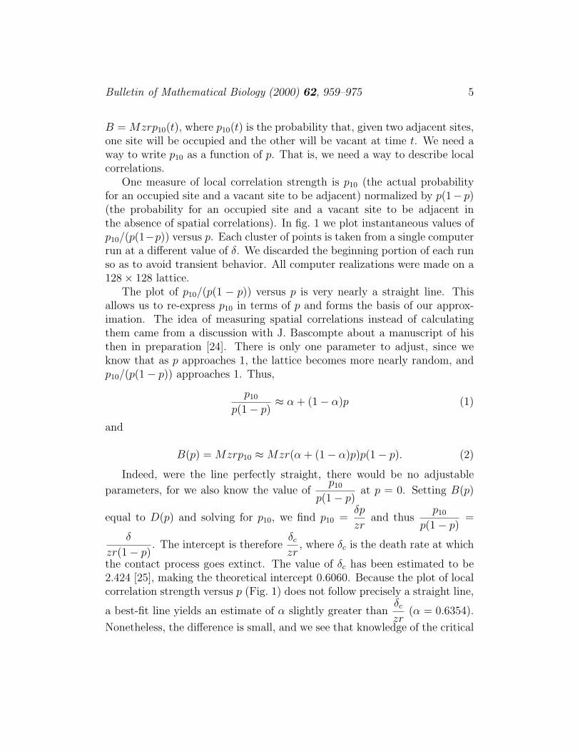
One measure of local correlation strength is p10 (the actual probabilityfor an occupied site and a vacant site to be adjacent) normalized by p(1− p)(the probability for an occupied site and a vacant site to be adjacent inthe absence of spatial correlations). In fig. 1 we plot instantaneous values ofp10/(p(1−p)) versus p. Each cluster of points is taken from a single computerrun at a different value of δ. We discarded the beginning portion of each runso as to avoid transient behavior. All computer realizations were made on a128× 128 lattice.

The plot of p10/(p(1 − p)) versus p is very nearly a straight line. Thisallows us to re-express p10 in terms of p and forms the basis of our approx-imation. The idea of measuring spatial correlations instead of calculatingthem came from a discussion with J. Bascompte about a manuscript of histhen in preparation [24]. There is only one parameter to adjust, since weknow that as p approaches 1, the lattice becomes more nearly random, andp10/(p(1− p)) approaches 1. Thus,

p10

p(1− p)≈ α + (1− α)p (1)

and

B(p) = Mzrp10 ≈Mzr(α + (1− α)p)p(1− p). (2)

Indeed, were the line perfectly straight, there would be no adjustable

parameters, for we also know the value ofp10

p(1− p)at p = 0. Setting B(p)

equal to D(p) and solving for p10, we find p10 =δp

zrand thus

p10

p(1− p)=

δ

zr(1− p). The intercept is therefore

δc

zr, where δc is the death rate at which

the contact process goes extinct. The value of δc has been estimated to be2.424 [25], making the theoretical intercept 0.6060. Because the plot of localcorrelation strength versus p (Fig. 1) does not follow precisely a straight line,

a best-fit line yields an estimate of α slightly greater thanδc

zr(α = 0.6354).

Nonetheless, the difference is small, and we see that knowledge of the critical


value of δ almost entirely specifies the local correlation structure.We are not always blessed with knowledge of the critical point. However,

it is straightforward to estimate α from a linear regression, and as long asthe relation between local correlation strength and p is nearly linear, we caneven base that regression solely on measurements at high density. This isconvenient for models with critical points at p = 0 since systems settle to aquasi-stationary state much faster when they are far from a critical point,and so simulations are less time-consuming at high density. As an example,fig. 1 shows regressions based on all of the data and on p > 0.6, yieldingα = 0.6354 and 0.6571, respectively. Both regressions are constrained topass through (1, 1).

2.2 Predictions

Having found an approximate restatement of the contact process in terms ofa stochastic birth-death process, we can now rapidly calculate the mean pop-ulation density, the population variance, and first passage time distributionsfor the population to reach low thresholds. (For concreteness, we interpretthe contact process as describing the spatial spread of a single population inthe remainder of this section and in the following section. Thus, “popula-tion” refers to the number of occupied sites, and “population density” refersto the fraction of occupied sites.) The mean population density can be wellapproximated as the equilibrium density of a deterministic model with thesame birth and death rates [23]. Setting the global birthrate, B(p), equal tothe global death rate, D(p), we obtain

p∗ =zr(2α− 1)−

√zr(zr − 4δ(1− α))

2zr(α− 1)(3)

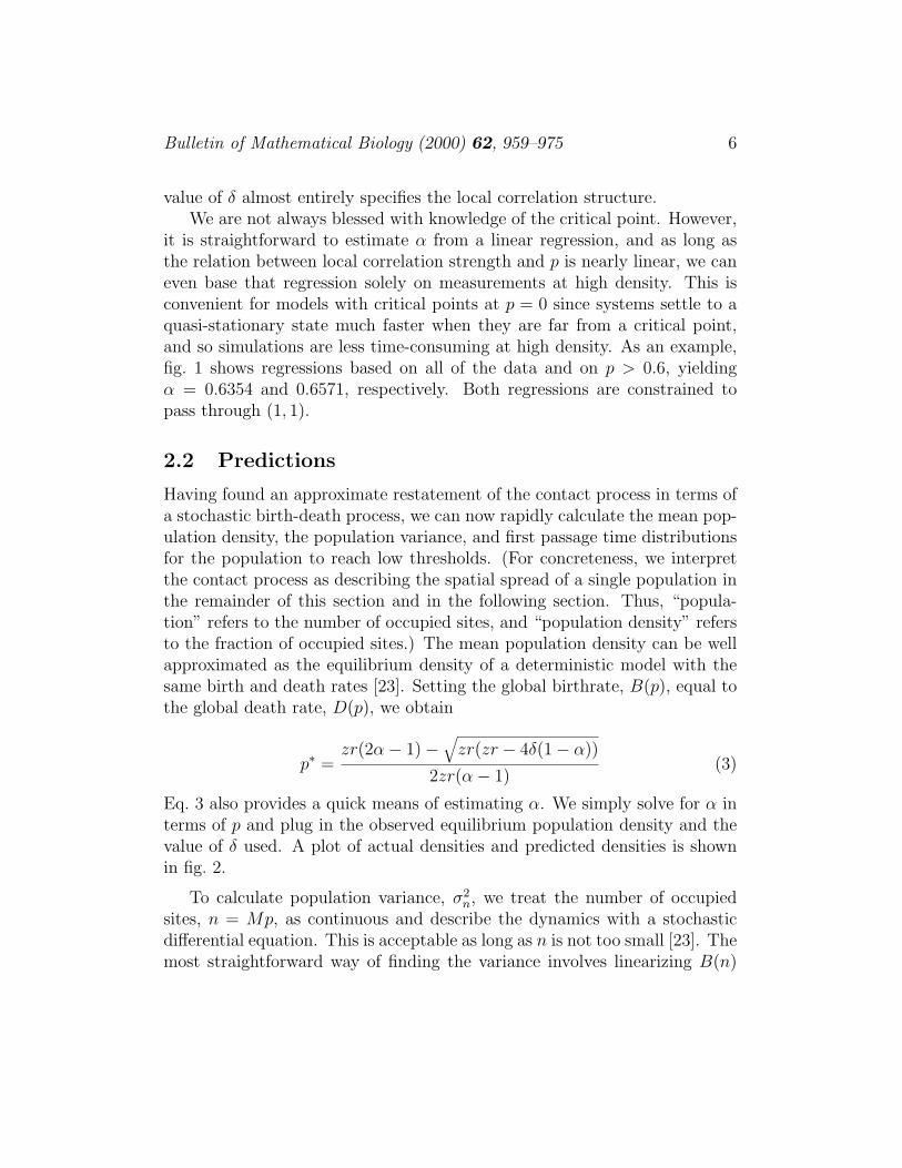
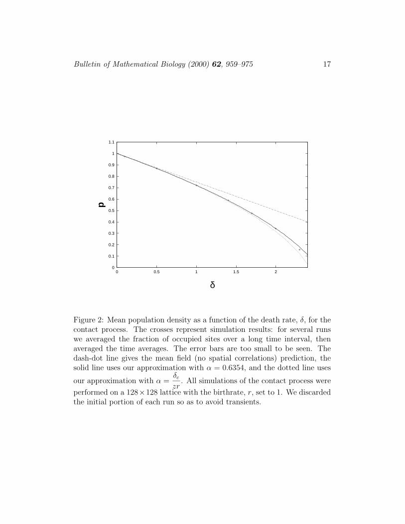
Eq. 3 also provides a quick means of estimating α. We simply solve for α interms of p and plug in the observed equilibrium population density and thevalue of δ used. A plot of actual densities and predicted densities is shownin fig. 2.

To calculate population variance, σ2n, we treat the number of occupied

sites, n = Mp, as continuous and describe the dynamics with a stochasticdifferential equation. This is acceptable as long as n is not too small [23]. Themost straightforward way of finding the variance involves linearizing B(n)


and D(n) about equilibrium and is detailed in a number of sources [23, 26, 27].The general result is that

σ2n =

Q

2a, (4)

where Q = B(n∗)+D(n∗) and a = − ∂

∂n(B(n)−D(n))

∣∣∣∣∣n=n∗

. The variance is

thus determined by a balance between transition rates (Q), which determinehow easily the system jumps away from equilibrium, and the response rateto perturbations (a), which determines how rapidly the system is draggedback to equilibrium. For our system

σ2n =

M [(α− 1)p2 + (1− 2α)p + α]

2(1− α)p + 2α− 1. (5)

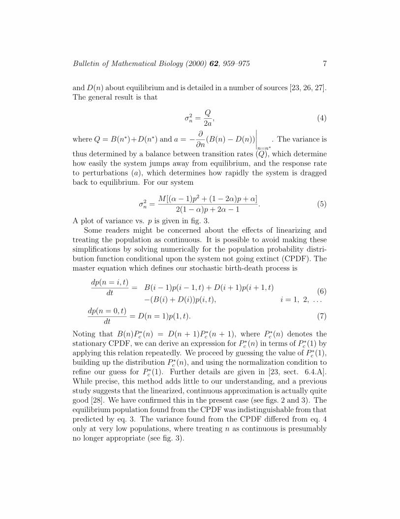
A plot of variance vs. p is given in fig. 3.Some readers might be concerned about the effects of linearizing and

treating the population as continuous. It is possible to avoid making thesesimplifications by solving numerically for the population probability distri-bution function conditional upon the system not going extinct (CPDF). Themaster equation which defines our stochastic birth-death process is

dp(n = i, t)

dt= B(i− 1)p(i− 1, t) + D(i + 1)p(i + 1, t)

−(B(i) + D(i))p(i, t), i = 1, 2, . . .(6)

dp(n = 0, t)

dt= D(n = 1)p(1, t). (7)

Noting that B(n)P ∗c (n) = D(n + 1)P ∗

c (n + 1), where P ∗c (n) denotes the

stationary CPDF, we can derive an expression for P ∗c (n) in terms of P ∗

c (1) byapplying this relation repeatedly. We proceed by guessing the value of P ∗

c (1),building up the distribution P ∗

c (n), and using the normalization condition torefine our guess for P ∗

c (1). Further details are given in [23, sect. 6.4.A].While precise, this method adds little to our understanding, and a previousstudy suggests that the linearized, continuous approximation is actually quitegood [28]. We have confirmed this in the present case (see figs. 2 and 3). Theequilibrium population found from the CPDF was indistinguishable from thatpredicted by eq. 3. The variance found from the CPDF differed from eq. 4only at very low populations, where treating n as continuous is presumablyno longer appropriate (see fig. 3).


When investigating a stochastic model, our most pressing question is oftenhow long will the system persist? While the ratio of variance to mean canprovide a rough estimate of viability (see for example [27]), a more preciseapproach is to calculate a first passage time distribution (FPTD) – that is, aprobability distribution for the time at which the population first dips belowa given threshold. Having captured the dynamics of the contact processwith our expression for the birth rate, we use our approximation to presenta calculation of a first passage time distribution.

To calculate an FPTD to threshold S, we add to the equations definingour stochastic birth-death process (eq. 6) an absorbing boundary at S:

dp(n = S, t)

dt= D(n = S + 1)p(S + 1, t) (8)

For our initial condition, we set p(n = Mp∗, t = 0) = 1 and p(n 6= Mp∗, t =0) = 0, representing an ensemble in which all replicates begin with populationequal to the equilibrium value.

Calculation of the FPTD is very sensitive to the value and slope of thepopulation distribution at S. Unfortunately, when we estimate α from alinear regression, as described in section 2.1, the resulting prediction for thepopulation distribution is not sufficiently accurate to make a good predictionof the FPTD. However, the population distribution is very nearly Gaussian aslong as δ is not too close to the critical point, and for a Gaussian distribution,specifying the derivative or the value at any point fixes α. Therefore, wehave simulated the contact process for δ = 2 and fit the resulting populationdistribution to a Gaussian curve. All runs were started with population equalto the equilibrium value, so as to be consistent with the initial conditionsused in our differential equations (eq. 6). We found the derivative of ourfitted Gaussian at S = 669, a population three standard deviations belowthe equilibrium value, and from this determined α. The change in α was

not great: the value of α determined from a linear regression ofp10

p(1− p)on

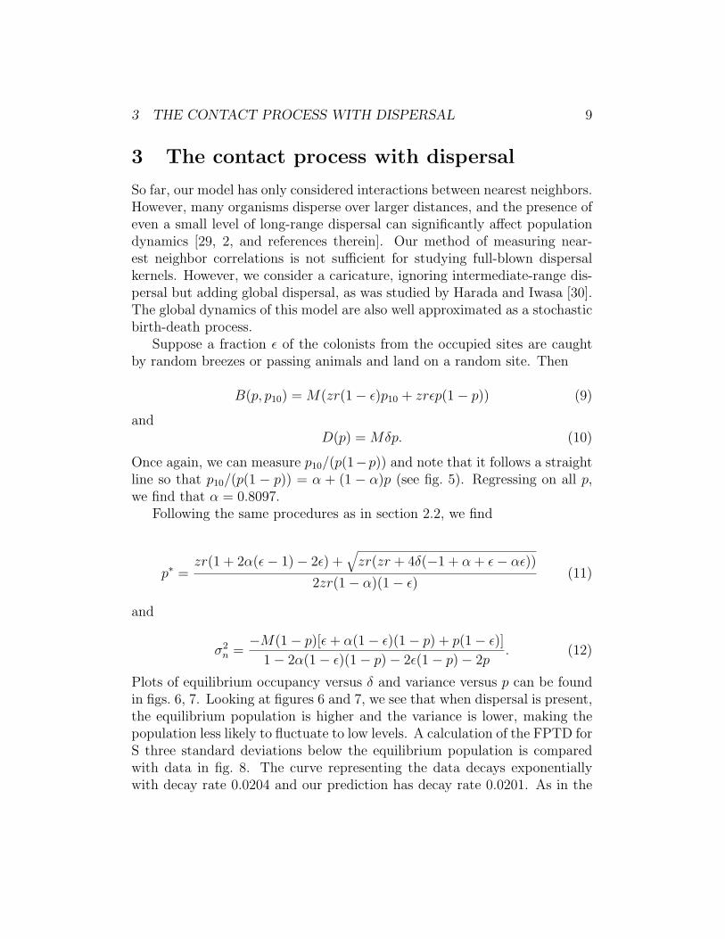
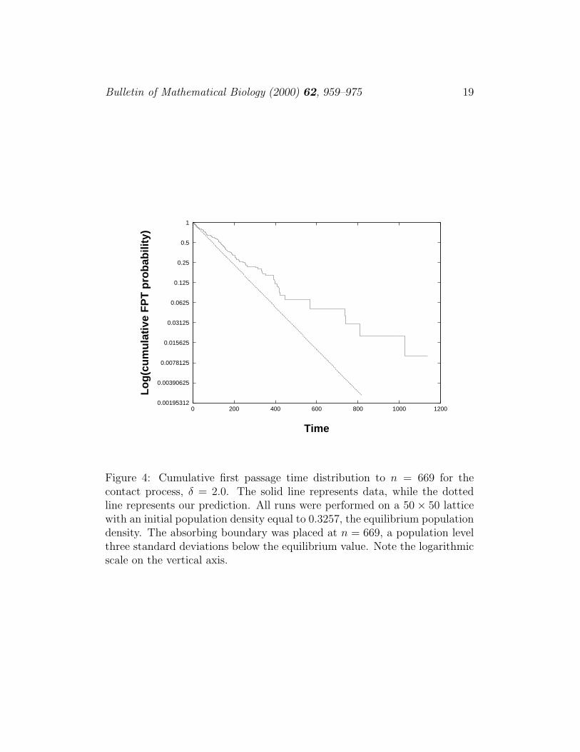
p was 0.6354, while the value of α obtained in the present case was 0.6208.We obtained similar results when we determined α by fixing the value of thepopulation distribution at S instead of its slope. The resulting predictionof the FPTD is reasonably good given the high sensitivity to α. The trueFPTD declines exponentially with decay rate 0.00517. Our prediction hasdecay rate 0.0073. A plot comparing our predictions with data is given infig. 4.

3 THE CONTACT PROCESS WITH DISPERSAL 9

3 The contact process with dispersal

So far, our model has only considered interactions between nearest neighbors.However, many organisms disperse over larger distances, and the presence ofeven a small level of long-range dispersal can significantly affect populationdynamics [29, 2, and references therein]. Our method of measuring near-est neighbor correlations is not sufficient for studying full-blown dispersalkernels. However, we consider a caricature, ignoring intermediate-range dis-persal but adding global dispersal, as was studied by Harada and Iwasa [30].The global dynamics of this model are also well approximated as a stochasticbirth-death process.

Suppose a fraction ε of the colonists from the occupied sites are caughtby random breezes or passing animals and land on a random site. Then

B(p, p10) = M(zr(1− ε)p10 + zrεp(1− p)) (9)

andD(p) = Mδp. (10)

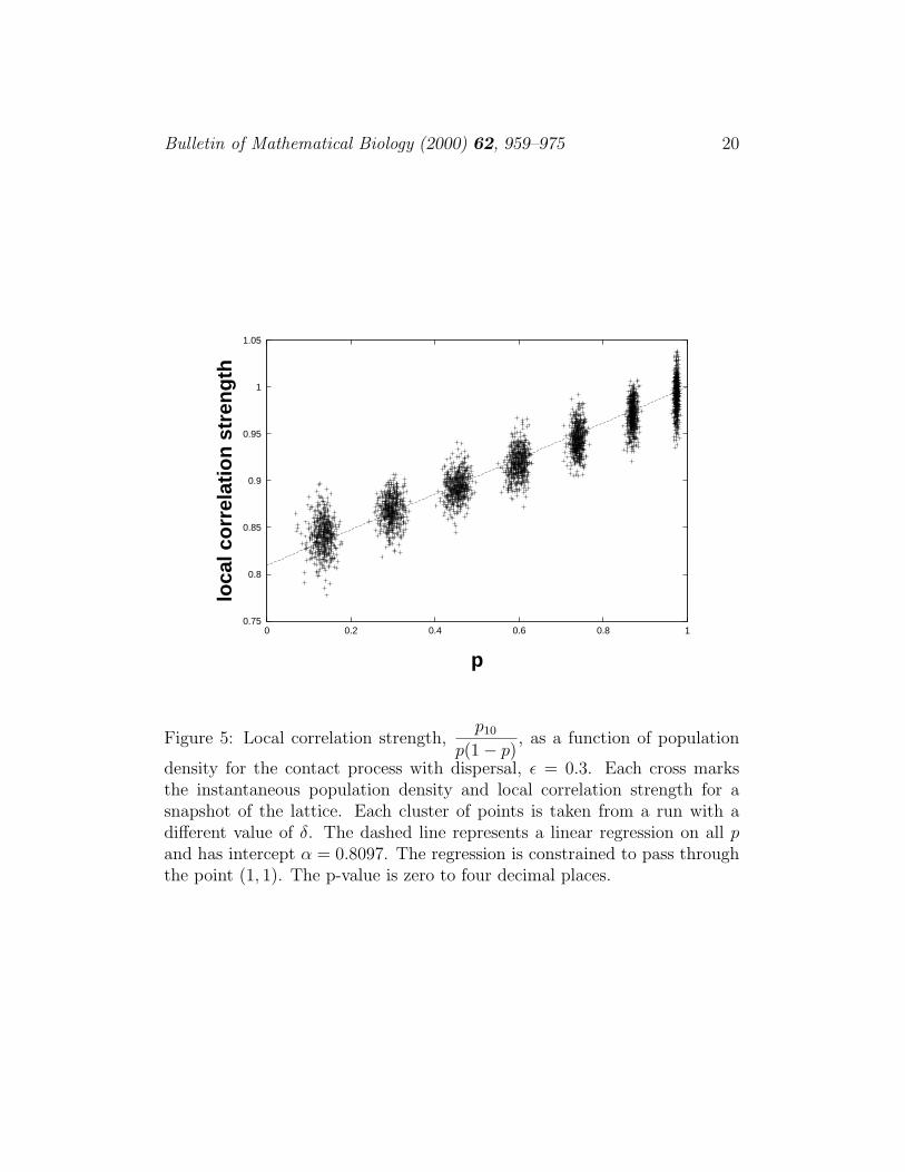
Once again, we can measure p10/(p(1−p)) and note that it follows a straightline so that p10/(p(1 − p)) = α + (1 − α)p (see fig. 5). Regressing on all p,we find that α = 0.8097.

Following the same procedures as in section 2.2, we find

p∗ =zr(1 + 2α(ε− 1)− 2ε) +

√zr(zr + 4δ(−1 + α + ε− αε))

2zr(1− α)(1− ε)(11)

and

σ2n =

−M(1− p)[ε + α(1− ε)(1− p) + p(1− ε)]

1− 2α(1− ε)(1− p)− 2ε(1− p)− 2p. (12)

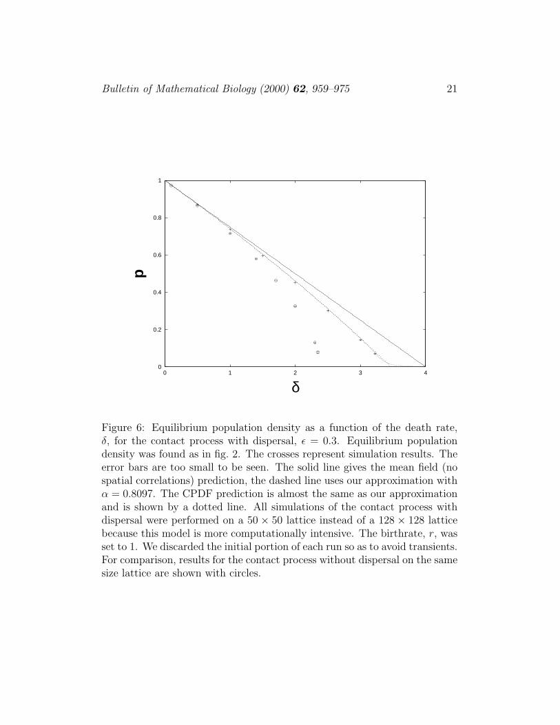
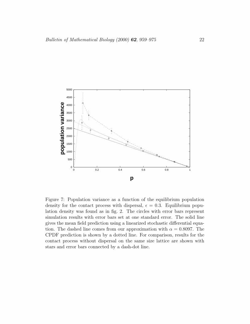
Plots of equilibrium occupancy versus δ and variance versus p can be foundin figs. 6, 7. Looking at figures 6 and 7, we see that when dispersal is present,the equilibrium population is higher and the variance is lower, making thepopulation less likely to fluctuate to low levels. A calculation of the FPTD forS three standard deviations below the equilibrium population is comparedwith data in fig. 8. The curve representing the data decays exponentiallywith decay rate 0.0204 and our prediction has decay rate 0.0201. As in the


last section, we used a value of α designed to give us the correct derivative ofthe population distribution with respect to n at the boundary. Comparingwith fig. 4, we see that the presence of dispersal significantly reduces firstpassage times to population levels an equal number of standard deviationsbelow the equilibrium value.

4 Discussion

Spatial correlations can strongly influence population dynamics. However,describing the effects of spatial correlations mathematically is difficult. Equa-tions for first-order moments rely on second-order moments; equations forsecond-order moments rely on third-order moments. The cascade of equa-tions needs to be truncated at some point, but it is difficult to do so withoutlosing a lot of information.

We avoid ad hoc closure methods by measuring the relation between thesecond-order moment p10 and the first-order moment p from simulations. Bymore accurately estimating p10, we are able to substantially improve upon thepredictions of moment closure schemes such as pair approximations. Sincethe interaction rules for our models depend only on nearest neighbors, in-formation about second-order moments fully specifies the dynamics. Havingcaptured the effects of space in the relation between p10 and p, we use this re-lation to create a nonspatial description of the contact process as a stochasticbirth-death process. We are then able to apply the many techniques availablefor analyzing stochastic birth-death processes to obtain predictions for equi-librium occupancy, occupancy variance, and first passage time distributions.

Our method characterizes spatial correlations better than pair approxima-tions or even “improved pair approximations” [15, 31]; however, our greatestadvantage over these methods is not our greater numerical accuracy but theease with which we can consider inherently stochastic quantities such as vari-ance and first passage time distributions. It is possible to add appropriatelyderived noise terms to pair approximation equations, but working with theresulting equations is laborious, it is nearly impossible to derive simple ex-pressions for quantities such as the variance, and improvements over methodswhich ignore spatial correlations are disappointingly small [32]. In contrast,our method yields insights into the mechanisms by which spatial correlationsaffect stochastic quantities.

As an example, consider the variance of the contact process without dis-


persal. Ignoring spatial correlations causes us to greatly underestimate thevariance. (Compare the mean field prediction (no spatial correlations) to thedata in fig. 3.) However, mean field theory overestimates the birth rate, sinceit ignores the tendency for occupied sites to cluster and increase crowding.This would naively lead us to expect a variance that is too large, since thesystem can jump away from equilibrium more rapidly. However, as we notedin section 2.2, variance is determined by the balance between this turnover

rate and a response rate, represented by − ∂

∂n(B(n)−D(n))

∣∣∣∣∣n=n∗

, which

measures how quickly the system returns to equilibrium after a fluctuation.By comparing the mean field birth rate, Mzrp(1− p), and the birth rate wederived by our method (eq. 2), we see that mean field theory overestimatesthe response rate. That is, the mean field variance is too small because ignor-ing spatial correlations causes us to overestimate the response rate even moredrastically than the turnover rate. Furthermore, we can see that the overlylarge birth rate is ultimately the source of the error in the response rate. Thebirth rate must of course be zero for a completely empty or completely fulllattice. Because mean field theory predicts too high a birth rate in betweenthese two extremes, the birth rate shoots up too rapidly as occupancy in-creases from zero and plummets too rapidly as occupancy approaches one,

making

∣∣∣∣∣∂B

∂p

∣∣∣∣∣ too large.

While we have focused on the contact process, this technique could beapplied to single-species models whose interactions depend on the state ofsurrounding sites in more complicated ways. For example, Wilson et al.’smussel model [33] contains a “safety in numbers” term. Mussels with fewerthan three neighbors are deemed vulnerable to wave action and have a highermortality rate. In this case, we would need to measure not pair probabilitiesbut probabilities for various configurations of the entire neighborhood. Al-though straightforward, this procedure can generate an unwieldy number ofparameters. For each new configuration that is associated with an interac-tion, we need to measure the probability of that configuration as a functionof p, which adds parameters. Moreover, not all of these functions may bewell approximated by a line, which adds further parameters.

The technique we have used to analyze the contact process may or maynot be extendable to multi-species models with nearest neighbor interactions,such as predator-prey models and susceptible-infected-recovered (SIR) epi-demic models. The difficulty stems from the presence of multiple independent


variables. Instead of relating spatial correlations to equilibrium occupancyand fitting a curve, we must relate spatial correlations to the equilibriumoccupancies of each species and fit a surface.

There remain a few caveats. Care needs to be taken in regions of metasta-bility. If there are two stable states, then even if one is always the eventualfavorite, the probability distribution function will be bimodal. The systemtrajectory will be subject to competing attractions to the two equilibria [23].Predicting variance from linearized stochastic differential equations, on theother hand, assumes that fluctuations are always drawn back to the sameequilibrium. This situation results in a Gaussian distribution (assuming lin-earized interactions).

The method we have presented is also not appropriate for examiningmetapopulations with only a few patches. In switching to differential equa-tions, we assumed that we could treat the number of occupied sites as con-tinuous. This assumption breaks down when the number of occupied sitesis small. Small systems also tend to be dominated by edge effects, whereaswe have assumed that the proportion of sites with fewer than z neighbors isnegligible.

Finally, the relation we have measured between p10 and p is valid nearequilibrium only. This means it is not appropriate for nonequilibrium situa-tions such as invading waves. On the other hand, Ellner et al. have presentedan invasion speed prediction for the contact process that uses simple modi-fications of equilibrium spatial correlations [34]. Their estimate of p10 comesfrom a pair approximation. We have tried substituting ours instead but foundthat it did not significantly improve their prediction. Evidently, the error inp10 is less important than the error introduced by using modified equilibriumvalues to describe spatial correlations in the wavefront.

5 Acknowledgments

We thank Jordi Bascompte, Benjamin Bolker, Douglas Donalson, ParviezHosseini, Timothy Keitt, Bruce Kendall, and Daniel Rabinowitz for helpfuldiscussions. One of us (RES) is grateful for financial support from NSFgrants BIR94-13141 and GER93-54870.

REFERENCES 13

References

[1] M. Keeling. Spatial models of interacting populations. In JacquelineMcGlade, editor, Advanced Ecological Theory: Principles and Applica-tions, pages 64–99. Blackwell Science, Oxford, 1999.

[2] P. Kareiva. Population dynamics in spatially complex environments:Theory and data. Philosophical Transactions of the Royal Society ofLondon B Biological, 330(1257):175–190, 1990.

[3] I. Hanski. Coexistence of competitors in patchy environment. Ecology,64:493–500, 1983.

[4] M. Slatkin. Competition and regional coexistence. Biometrika, 55:128–134, 1974.

[5] G. Nachman. Systems analysis of acarine predator-prey interactions:II. the role of spatial processes in system stability spatial processes insystem stability. Journal of Animal Ecology, 56(1):267–282, 1987.

[6] B. P. Zeigler. Persistence and patchiness of predator-prey systems in-duced by discrete event population exchange mechanisms. Journal ofTheoretical Biology, 67:687–713, 1977.

[7] J. D. Reeve. Environmental variability, migration, and persistence inhost-parasitoid systems systems. American Naturalist, 132(6):810–836,1988.

[8] J. Allen. Mathematical models of species interactions in time and space.American Naturalist, 109:319–342, 1975.

[9] R. Durrett and S. A. Levin. Stochastic spatial models: A user’s guide toecological applications. Philosophical Transactions of the Royal Societyof London B Biological, 343(1305):329–350, 1994.

[10] J. P. Barkham and C. E. Hance. Population dynamics of the wild daffodil(narcissus pseudonarcissus) III. implications of a computer model of1000 years of population change. Journal of Ecology, 70:323–344, 1982.

[11] T. Ohtsuki and T. Keyes. Kinetic growth percolation: epidemic pro-cesses with immunization. Physical Review A, 33(2):1223–32, February1986.

REFERENCES 14

[12] Shane A. Richards, William G. Wilson, and Joshua E. S. Socolar. Se-lection for short-lived and offspring-limited individuals in a spatially-structured population which is subject to localized disturbances. Un-published manuscript, 1999.

[13] E. McCauley, W. G. Wilson, and A. M. De Roos. Dynamicsof age-structured and spatially structured predator-prey interactionsindividual-based models and population-level formulations. AmericanNaturalist, 142(3):412–442, 1993.

[14] R. Levins. Some demographic and genetic consequences of environmen-tal heterogeneity for biological control. The Bulletin of the EntomologicalSociety of America, 15:237–240, 1969.

[15] K. Sato, H. Matsuda, and A. Sasaki. Pathogen invasion and host extinc-tion in lattice structured populations. Journal of Mathematical Biology,32(3):251–268, 1994.

[16] Y. Harada, H. Ezoe, Y. Iwasa, H. Matsuda, and K. Sato. Populationpersistence and spatially limited social interaction. Theoretical Popula-tion Biology, 48(1):65–91, 1995.

[17] D. A. Rand. Correlation equations and pair approximations for spatialecologies. In Jacqueline McGlade, editor, Advanced Ecological Theory:Principles and Applications, pages 100–142. Blackwell Science, Oxford,1999.

[18] R. Dickman. Kinetic phase transitions in a surface-reaction model:mean-field theory. Physical Review A, 34(5):4246–50, November 1986.

[19] H. Matsuda, N. Ogita, A. Sasaki, and K. Sato. Statistical mechanicsof population-the lattice Lotka-Volterra model. Progress of TheoreticalPhysics, 88(6):1035–49, December 1992.

[20] K. G. Wilson. The renormalization group and critical phenomena. Re-views of Modern Physics, 55:583–600, 1983. Nobel Prize Lecture.

[21] M. E. Fisher. Renormalization group theory: Its basis and formulationin statistical physics. Reviews of Modern Physics, 70(2):653–81, April1998.

REFERENCES 15

[22] N. G. van Kampen. Stochastic Processes in Physics and Chemistry.North-Holland, Amsterdam, 1981.

[23] R. M. Nisbet and W. S. C. Gurney. Modelling Fluctuating Populations.John Wiley & Sons, New York, 1982.

[24] Jordi Bascompte. Aggregate statistical measures and metapopulationdynamics. Submitted to Journal of Animal Ecology, 1999.

[25] M. Katori and N. Konno. Correlation inequalities and lower bounds forthe critical value lambda /sub c/ of contact processes. Journal of thePhysical Society of Japan, 59(3):877–87, March 1990.

[26] Eric Renshaw. Modelling Biological Populations in Space and Time.Cambridge University Press, New York, 1991.

[27] W. S. C. Gurney and R. M. Nisbet. Single-species population fluctua-tions in patchy environments. The American Naturalist, 112(988):1075–1090, 1978.

[28] R. M. Nisbet, W. S. C. Gurney, and M. A. Pettipher. An evaluation oflinear models of population fluctuations. Journal of Theoretical Biology,68:143–160, 1977.

[29] Nanako Shigesada and Kohkichi Kawasaki. Biological Invasions: Theoryand Practice. Oxford University Press, New York, 1997.

[30] Yuko Harada and Yoh Iwasa. Lattice population dynamics for plantswith dispersing seeds and vegetative propagation. Researches on Popu-lation Ecology (Kyoto), 36(2):237–249, 1994.

[31] Minus van Baalen and David A Rand. The unit of selection in vis-cous populations and the evolution of altruism. Journal of TheoreticalBiology, 193(4):631–648, August 1998.

[32] Robin E. Snyder. Effects of spatial correlations and fluctuations onpopulation dynamics. Ph.D. thesis, in prep., University of California,Santa Barbara, 2000.

[33] W G Wilson, R M Nisbet, A H Ross, C Robles, and R A Desharnais.Abrupt population changes along smooth environmental gradients. Bul-letin of Mathematical Biology, 58(5):907–922, 1996.


[34] Stephen P. Ellner, Akira Sasaki, Yoshihiro Haraguchi, and HirotsuguMatsuda. Speed of invasion in lattice population models: Pair-edgeapproximation. Journal of Mathematical Biology, 36(5):469–484, 1998.

0.55

0.6

0.65

0.7

0.75

0.8

0.85

0.9

0.95

1

1.05

0 0.2 0.4 0.6 0.8 1

loca

l co

rrel

atio

n s

tren

gth

p

Figure 1: Local correlation strength,p10

p(1− p), as a function of population

density for the contact process. Each cross marks the instantaneous pop-ulation density and local correlation strength for a snapshot of the lattice.Each cluster of points is taken from a run with a different value of δ. Thelong dashed line represents a linear regression on p > 0.6 and has interceptα = 0.6571. The short dashed line represents a linear regression on all p andhas intercept α = 0.6354. Both regressions are constrained to pass throughthe point (1, 1). Both p-values are zero to four decimal places.


0

0.1

0.2

0.3

0.4

0.5

0.6

0.7

0.8

0.9

1

1.1

0 0.5 1 1.5 2

p

δ

Figure 2: Mean population density as a function of the death rate, δ, for thecontact process. The crosses represent simulation results: for several runswe averaged the fraction of occupied sites over a long time interval, thenaveraged the time averages. The error bars are too small to be seen. Thedash-dot line gives the mean field (no spatial correlations) prediction, thesolid line uses our approximation with α = 0.6354, and the dotted line uses

our approximation with α =δc

zr. All simulations of the contact process were

performed on a 128×128 lattice with the birthrate, r, set to 1. We discardedthe initial portion of each run so as to avoid transients.


0

5000

10000

15000

20000

25000

30000

35000

40000

45000

50000

0 0.2 0.4 0.6 0.8 1

po

pu

lati

on

var

ian

ce

p

Figure 3: Population variance as a function of the equilibrium populationdensity for the contact process. Equilibrium population density was foundas in fig. 2. The crosses represent simulation results with error bars set atone standard error. Horizontal error bars are too small to see. The solidline gives the mean field prediction using a linearized stochastic differentialequation, while the dotted line gives the prediction using the CPDF. The

dashed line comes from our approximation with α =δc

zrand the dash-dot

line comes from our approximation with α = 0.6354.


0.00195312

0.00390625

0.0078125

0.015625

0.03125

0.0625

0.125

0.25

0.5

1

0 200 400 600 800 1000 1200

Lo

g(c

um

ula

tive

FP

T p

rob

abili

ty)

Time

Figure 4: Cumulative first passage time distribution to n = 669 for thecontact process, δ = 2.0. The solid line represents data, while the dottedline represents our prediction. All runs were performed on a 50× 50 latticewith an initial population density equal to 0.3257, the equilibrium populationdensity. The absorbing boundary was placed at n = 669, a population levelthree standard deviations below the equilibrium value. Note the logarithmicscale on the vertical axis.


0.75

0.8

0.85

0.9

0.95

1

1.05

0 0.2 0.4 0.6 0.8 1

loca

l co

rrel

atio

n s

tren

gth

p

Figure 5: Local correlation strength,p10

p(1− p), as a function of population

density for the contact process with dispersal, ε = 0.3. Each cross marksthe instantaneous population density and local correlation strength for asnapshot of the lattice. Each cluster of points is taken from a run with adifferent value of δ. The dashed line represents a linear regression on all pand has intercept α = 0.8097. The regression is constrained to pass throughthe point (1, 1). The p-value is zero to four decimal places.


0

0.2

0.4

0.6

0.8

1

0 1 2 3 4

p

δ

Figure 6: Equilibrium population density as a function of the death rate,δ, for the contact process with dispersal, ε = 0.3. Equilibrium populationdensity was found as in fig. 2. The crosses represent simulation results. Theerror bars are too small to be seen. The solid line gives the mean field (nospatial correlations) prediction, the dashed line uses our approximation withα = 0.8097. The CPDF prediction is almost the same as our approximationand is shown by a dotted line. All simulations of the contact process withdispersal were performed on a 50 × 50 lattice instead of a 128 × 128 latticebecause this model is more computationally intensive. The birthrate, r, wasset to 1. We discarded the initial portion of each run so as to avoid transients.For comparison, results for the contact process without dispersal on the samesize lattice are shown with circles.


0

500

1000

1500

2000

2500

3000

3500

4000

4500

5000

0 0.2 0.4 0.6 0.8 1

po

pu

lati

on

var

ian

ce

p

Figure 7: Population variance as a function of the equilibrium populationdensity for the contact process with dispersal, ε = 0.3. Equilibrium popu-lation density was found as in fig. 2. The circles with error bars representsimulation results with error bars set at one standard error. The solid linegives the mean field prediction using a linearized stochastic differential equa-tion. The dashed line comes from our approximation with α = 0.8097. TheCPDF prediction is shown by a dotted line. For comparison, results for thecontact process without dispersal on the same size lattice are shown withstars and error bars connected by a dash-dot line.


0.0078125

0.015625

0.03125

0.0625

0.125

0.25

0.5

1

0 50 100 150 200 250

Lo

g(c

um

ula

tive

FP

T p

rob

abili

ty)

Time

Figure 8: Cumulative first passage time distribution to n = 669 for thecontact process with dispersal, δ = 2.0 and ε = 0.3. The solid line representsdata, while the dotted line represents our prediction. All runs were performedon a 50 × 50 lattice with an initial population density equal to 0.4519, theequilibrium population density. The absorbing boundary was placed at n =1016, a population level three standard deviations below the equilibriumvalue. Note the logarithmic scale on the vertical axis.

Documents

Spatial structure and ﬂuctuations in the contact process