COMPARATIVE ANALYSIS OF SPATIAL AND · PDF file · 2006-07-26CHRISTOPH MATULLA,a,b,* EDOUARD K. PENLAP,a,c PATRICK HAASb and ... e-mail: matulla@ ... detection of climatic ﬂuctuations;

INTERNATIONAL JOURNAL OF CLIMATOLOGY

Int. J. Climatol. 23: 1577–1588 (2003)

Published online in Wiley InterScience (www.interscience.wiley.com). DOI: 10.1002/joc.960

COMPARATIVE ANALYSIS OF SPATIAL AND SEASONAL VARIABILITY:AUSTRIAN PRECIPITATION DURING THE 20TH CENTURY

CHRISTOPH MATULLA,a,b,* EDOUARD K. PENLAP,a,c PATRICK HAASb and HERBERT FORMAYERb

a Institute for Coastal Research, GKSS Research Centre, Max-Planck-Straße 1, Geesthacht, Germanyb Institute of Meteorology and Physics, University of Natural Resources and Applied Life Sciences, Turkenschanzstrasse 18,

Vienna, Austriac Atmospheric Sciences Laboratory, Department of Physics, Faculty of Sciences, University of Yaounde I, Yaounde, Cameroon

Received 26 March 2003Revised 28 July 2003

Accepted 28 July 2003

ABSTRACT

The purpose of this investigation is to demonstrate the usability of objective methods to study the variability ofprecipitation and hence to contribute to a better understanding of spatial and seasonal variability of Austria’s precipitationclimate during the 20th century.

This will be achieved by regionalizing the intra-annual variability of seasonal precipitation distributions during threenon-overlapping 33 year samples (1901–33, 1934–66, 1967–99). Monthly precipitation totals were extracted at 31Austrian stations from a homogenized long-term climate dataset provided by the Austrian weather service. Three statisticaltechniques, namely cluster analysis (CLA), rotated empirical orthogonal functions (REOFs) and an unsupervised learningprocedure of artificial neural networks (ANNs), were utilized to find homogeneous precipitation regions.

The results of summer (June, July, August (JJA)) and winter (December, January, February (DJF)) seasons arepresented. The resulting homogeneous precipitation regions depend on season, period and method in this order. Hence,differences introduced by using different methods are small compared with those inferred by investigating differentepisodes and especially with those related to the seasons.

During winter, three homogeneous precipitation regions are found, independent from the period considered. Theseregions can be assigned to different airflows dominating Austria’s climate and triggering precipitation events during thecold season. The situation during summer is more complicated. Thus, at least four clusters are necessary to record thecircumstances, which are caused by spatially inhomogeneous convective events such as thunderstorms. Copyright 2003Royal Meteorological Society.

KEY WORDS: homogeneous regions; REOFs; cluster analysis; ANNs; Austria’s precipitation climate

1. INTRODUCTION

Precipitation is one of the main climatic elements and its distribution can be highly variable in space and time,particularly over complex terrain. Long-term fluctuations of precipitation affect the composition of vegetationdirectly (Lexer et al., 2002). Hence, recording of past variations and simulation of future variations andchanges of homogeneous precipitation regions are principal tasks of climate research.

This work pursues two aims. First, to illustrate objective methods to detect homogeneous precipitationregions and thereby to contribute to a better understanding of the spatial and seasonal variability ofprecipitation climate in Austria. Second, to study precipitation behaviour during the 20th century. Thesegoals appear to be of value, since Austria’s precipitation climate is marked by complicated patterns of spatialand seasonal variability (Auer, 1993). Nevertheless, the results of the study are limited by the difficulties ofmeasuring precipitation in high mountains.

* Correspondence to: Christoph Matulla, Institute for Coastal Research, GKSS Research Centre, Max-Planck-Straße 1, Geesthacht,Germany; e-mail: [email protected]

Copyright 2003 Royal Meteorological Society

1578 C. MATULLA ET AL.

Stations

< 750 m

> 2250 m

750 m − 1500 m1500 m − 2250 m

Topography of Austria

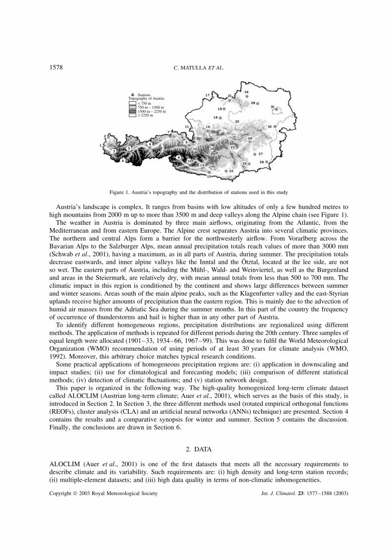
Figure 1. Austria’s topography and the distribution of stations used in this study

Austria’s landscape is complex. It ranges from basins with low altitudes of only a few hundred metres tohigh mountains from 2000 m up to more than 3500 m and deep valleys along the Alpine chain (see Figure 1).

The weather in Austria is dominated by three main airflows, originating from the Atlantic, from theMediterranean and from eastern Europe. The Alpine crest separates Austria into several climatic provinces.The northern and central Alps form a barrier for the northwesterly airflow. From Vorarlberg across theBavarian Alps to the Salzburger Alps, mean annual precipitation totals reach values of more than 3000 mm(Schwab et al., 2001), having a maximum, as in all parts of Austria, during summer. The precipitation totalsdecrease eastwards, and inner alpine valleys like the Inntal and the Otztal, located at the lee side, are notso wet. The eastern parts of Austria, including the Muhl-, Wald- and Weinviertel, as well as the Burgenlandand areas in the Steiermark, are relatively dry, with mean annual totals from less than 500 to 700 mm. Theclimatic impact in this region is conditioned by the continent and shows large differences between summerand winter seasons. Areas south of the main alpine peaks, such as the Klagenfurter valley and the east-Styrianuplands receive higher amounts of precipitation than the eastern region. This is mainly due to the advection ofhumid air masses from the Adriatic Sea during the summer months. In this part of the country the frequencyof occurrence of thunderstorms and hail is higher than in any other part of Austria.

To identify different homogeneous regions, precipitation distributions are regionalized using differentmethods. The application of methods is repeated for different periods during the 20th century. Three samples ofequal length were allocated (1901–33, 1934–66, 1967–99). This was done to fulfil the World MeteorologicalOrganization (WMO) recommendation of using periods of at least 30 years for climate analysis (WMO,1992). Moreover, this arbitrary choice matches typical research conditions.

Some practical applications of homogeneous precipitation regions are: (i) application in downscaling andimpact studies; (ii) use for climatological and forecasting models; (iii) comparison of different statisticalmethods; (iv) detection of climatic fluctuations; and (v) station network design.

This paper is organized in the following way. The high-quality homogenized long-term climate datasetcalled ALOCLIM (Austrian long-term climate; Auer et al., 2001), which serves as the basis of this study, isintroduced in Section 2. In Section 3, the three different methods used (rotated empirical orthogonal functions(REOFs), cluster analysis (CLA) and an artificial neural networks (ANNs) technique) are presented. Section 4contains the results and a comparative synopsis for winter and summer. Section 5 contains the discussion.Finally, the conclusions are drawn in Section 6.

2. DATA

ALOCLIM (Auer et al., 2001) is one of the first datasets that meets all the necessary requirements todescribe climate and its variability. Such requirements are: (i) high density and long-term station records;(ii) multiple-element datasets; and (iii) high data quality in terms of non-climatic inhomogeneities.

Copyright 2003 Royal Meteorological Society Int. J. Climatol. 23: 1577–1588 (2003)

PRECIPITATION VARIABILITY IN AUSTRIA 1579

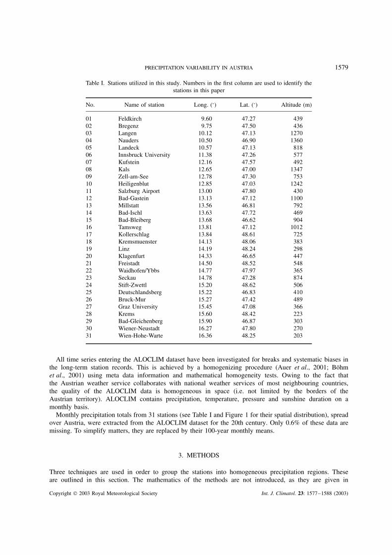
Table I. Stations utilized in this study. Numbers in the first column are used to identify thestations in this paper

No. Name of station Long. (°) Lat. (°) Altitude (m)

01 Feldkirch 9.60 47.27 43902 Bregenz 9.75 47.50 43603 Langen 10.12 47.13 127004 Nauders 10.50 46.90 136005 Landeck 10.57 47.13 81806 Innsbruck University 11.38 47.26 57707 Kufstein 12.16 47.57 49208 Kals 12.65 47.00 134709 Zell-am-See 12.78 47.30 75310 Heiligenblut 12.85 47.03 124211 Salzburg Airport 13.00 47.80 43012 Bad-Gastein 13.13 47.12 110013 Millstatt 13.56 46.81 79214 Bad-Ischl 13.63 47.72 46915 Bad-Bleiberg 13.68 46.62 90416 Tamsweg 13.81 47.12 101217 Kollerschlag 13.84 48.61 72518 Kremsmuenster 14.13 48.06 38319 Linz 14.19 48.24 29820 Klagenfurt 14.33 46.65 44721 Freistadt 14.50 48.52 54822 Waidhofen/Ybbs 14.77 47.97 36523 Seckau 14.78 47.28 87424 Stift-Zwettl 15.20 48.62 50625 Deutschlandsberg 15.22 46.83 41026 Bruck-Mur 15.27 47.42 48927 Graz University 15.45 47.08 36628 Krems 15.60 48.42 22329 Bad-Gleichenberg 15.90 46.87 30330 Wiener-Neustadt 16.27 47.80 27031 Wien-Hohe-Warte 16.36 48.25 203

All time series entering the ALOCLIM dataset have been investigated for breaks and systematic biases inthe long-term station records. This is achieved by a homogenizing procedure (Auer et al., 2001; Bohmet al., 2001) using meta data information and mathematical homogeneity tests. Owing to the fact thatthe Austrian weather service collaborates with national weather services of most neighbouring countries,the quality of the ALOCLIM data is homogeneous in space (i.e. not limited by the borders of theAustrian territory). ALOCLIM contains precipitation, temperature, pressure and sunshine duration on amonthly basis.

Monthly precipitation totals from 31 stations (see Table I and Figure 1 for their spatial distribution), spreadover Austria, were extracted from the ALOCLIM dataset for the 20th century. Only 0.6% of these data aremissing. To simplify matters, they are replaced by their 100-year monthly means.

3. METHODS

Three techniques are used in order to group the stations into homogeneous precipitation regions. Theseare outlined in this section. The mathematics of the methods are not introduced, as they are given in



various statistical publications (e.g. Haykin, 1994; von Storch and Zwiers, 1999). However, the main ideasare presented.

The methods utilized are: (i) a principal component analysis (PCA) performed on seasonal correlationmatrices of precipitation data followed by a varimax rotation (REOFs); (ii) a cluster analysis (CLA) and(iii) a subgroup of artificial neural networks (ANNs) using the process of ‘competitive learning’.

3.1. Rotated empirical orthogonal functions

Rotation was introduced to meteorology by Richman (1986) and its goal is to derive simple but meaningfulpatterns. Ehrendorfer (1987) used REOFs to identify homogeneous regions for summer and winter half-yearsfrom 1951 to 1980 in Austria. He utilized networks with somewhat less than 30 stations and found threeprecipitation regions of Austria for both winter and summer half-years. Widmann (1996) regionalized Swissprecipitation from 1961 to 1990 and Alpine precipitation from 1978 to 1991 using REOFs.

PCA is used to identify a low-dimensional subspace of the original data-space that contains most of itsvariability. This subspace is spanned by the leading eigenvectors, termed empirical orthogonal functions(EOFs). The rotation procedure usually follows a PCA in order to separate the noise from the signal.

The desired ‘simple’ patterns are obtained by applying an orthonormal transformation to the EOFs. Therequired transformation solves a variational problem, which minimizes a cost function (von Storch and Zwiers,1999). The form of the cost function characterizes the shape of the REOFs.

Simplicity can be achieved for the REOFs or their time coefficients, but not for both at the same time;hence, the REOFs can be orthogonal or the coefficients can be uncorrelated. In this study, the so-called‘varimax’ method (Richman, 1986) is used to determine the form of the cost function.

3.2. Cluster analysis

Woth (2001) used a hierarchical CLA to find homogeneous regions of winter (DJF) precipitation on theIberian Peninsula and in the south of France. Ramos (2001) investigated autumn and spring precipitationdistribution patterns in northeastern Spain for the period 1889–1999 by applying hierarchical and non-hierarchical CLA techniques. Jackson and Weinand (1994) classified tropical precipitation stations distributedover the globe, using PCA and a clustering procedure. They utilized daily data records of different lengths,ranging from 5 to >50 years.

The purpose of a CLA is to sort objects into clusters according to different aspects. Clusters areunits containing objects. Following Woth (2001), a hierarchical type of CLA is used to identify differenthomogeneous precipitation regions.

A hierarchical CLA is situated between two extreme states. One at its beginning, where every object formsa cluster on its own, and another at its end, where all objects are joined into one cluster. Between theseextremes the objects are onwardly aggregated into clusters. In this study, the objects under investigation arenormalized anomalies of seasonal precipitation totals at Austrian stations. CLA offers many possibilities ofgrouping objects. This wide choice corresponds to the ways of answering the following questions:

1. How can similarity between the objects/clusters be quantified?2. When should two objects/clusters be joined into one?

Both questions deal with fuzziness — different objects or clusters become indistinguishable with increasingfuzziness. In this work, the correlation coefficient was selected to quantify fuzziness and thereby to answerthe above questions. With reference to question 1, a high correlation coefficient between two objects accountsfor much similarity between them. With reference to question 2, two clusters are not joined together untilthe correlation coefficient between their most dissimilar objects is lower than the fuzziness considered. Thisintersection technique is called the ‘complete linkage method’. It does not combine different clusters untilthe Euclidean distance between the most dissimilar objects underruns a given value. The utilization of thecorrelation coefficient ρ advises the use of normalized anomalies (X, Y) as objects, mainly because it permits



the formulation of the correlation coefficient as a simple function of the distance:

ρ(X, Y) = 1 − 12 ||X − Y||2

An effective CLA should provide clusters inheriting a high degree of inner homogeneity and outer separation,i.e. the correlation coefficients between the objects inside the clusters should be high and between differentclusters the corresponding correlation coefficient should be low.

3.3. Self-organizing networks

ANNs have been used for a wide range of applications. Foody (1999), for example, used ANNs to classifyvegetation data in environmental sciences, Michaelides et al. (2001) and Hewitson and Crane (2002) appliedthem to the climatological domain. Michaelides et al. (2001) used ANNs to classify rainfall variability inCyprus. They found that ANNs perform more realistically than a CLA.

Self-organizing networks are a subgroup of ANNs intended to perform a mapping of arbitrarily distributeddata (input patterns) on a low-dimensional space. More precisely, it is an ‘unsupervised learning’ procedure.There are many types of self-organizing network applicable to a wide area of problems. Hewitson and Crane(2002) recently used ‘self-organizing feature maps’ to describe changes of synoptic circulation and discuss indetail their performance and application within the climatology domain. Here, another technique, ‘competitivelearning’ (Rumelhart and Zipser, 1985), which is related to ‘self-organizing feature maps’, is used. This kindof self-organizing network divides a set of input patterns into groups.

The architecture of the neural network used in this paper consists of an input layer containing n nodesand an output layer with n0 nodes, where n corresponds to the dimension of the input vector, which in ourcase equals the length of the time series, and n0 is the desired number of clusters. Each node of the outputlayer is connected to all nodes of the input layer through the connection weights. The input data are generallyarranged as a matrix of m × n dimension, where m and n denote the number of observations and variablesrespectively. The data are assigned to the output nodes through an iterative process. An iteration consists ofselecting an observation (input vector) at random, finding its ‘best matching’ output node (the one having thesmallest Euclidean distance with the input vector) and updating the connection weights. The updating formulais a function of one learning rate η. In total, there are two learning rates η and η

′(η � η

′), which are fixed

during the whole process: η is used to update the weights of the ‘best matching’ node and η′

for all others.η

′is used to prevent the situation of only one node being the ‘best matching’ node. If further iterations cause

no alteration of the compositions of each node, then the learning process is complete. All stations mappedonto the same node form a group.

4. RESULTS

4.1. Rotated empirical orthogonal functions

In this study, the seasonal totals at the stations in their standardized form are entered in the rotationapproach, which is explained in Section 3.

The first step is to perform a PCA on the standardized random variable, i.e. to diagonalize the correlationmatrix. The corresponding eigenvectors (EOFs) form an orthogonal basis and their time coefficients areuncorrelated. The resulting eigenvalues are utilized, via the so called ‘logarithm of eigenvalue plots’(Preisendorfer, 1988), to determine the dimension of the subspace containing the main fraction of variance.

In case of DJF, the subspaces spanned by the first three (four) EOFs contain more than 75% (80%) of theintra-annual variance. During the summer season (JJA), the first four (five) EOFs explain more than 65%(70%); see Table II.

However, the quality of the EOFs declines with increasing index; hence, including more and moreEOFs will not solve the problem. Von Storch and Hannoschock (1985) showed that the variance of theeigenvalue estimates is large and biased. In general, large eigenvalues are overestimated and small ones



Table II. Fraction of variance explained by the leading DJFand JJA EOFs

Period Explained variance (%)

DJF JJA

3EOFs 4EOFs 4EOFs 5EOFs

1901–33 77.4 81.9 70.8 74.81934–66 81.1 85.6 74.4 79.01967–99 76.2 81.9 67.4 72.3

are underestimated. These errors become considerably large if the degree of freedom exceeds the samplesize. Hence, it was decided to take the first three DJF EOFs and the first four JJA EOFs. Ehrendorfer(1987), who investigated the period 1951–80, took three EOFs for both the winter and summer half-years.Subsequently, the varimax rotation that provides the REOFs is applied. With respect to subsequent applications(e.g. downscaling), it was decided to keep the time coefficients of the rotated patterns uncorrelated, whichimplies that the REOFs are not orthogonal. Thus, the EOFs and their coefficients have to be renormalizedprior to rotation (von Storch and Zwiers, 1999).

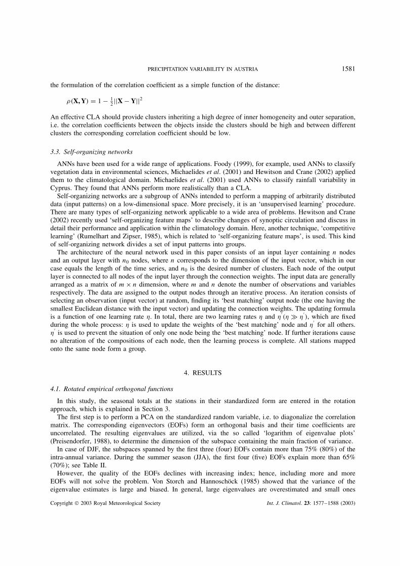
Stations that share the highest value at the same rotated vector are combined into one group. Hence,the maximum number of regions is given by the dimension of the subspace retained, i.e. three (four) forthe winter (summer) season. Figure 2 displays the regions found during the winter (left-hand side) and thesummer seasons (right-hand side).

4.2. Cluster analysis

As mentioned in Section 3, we apply the ‘complete linkage method’ as an intersection technique and thenormalized time series at the stations are entered in the cluster analysis.

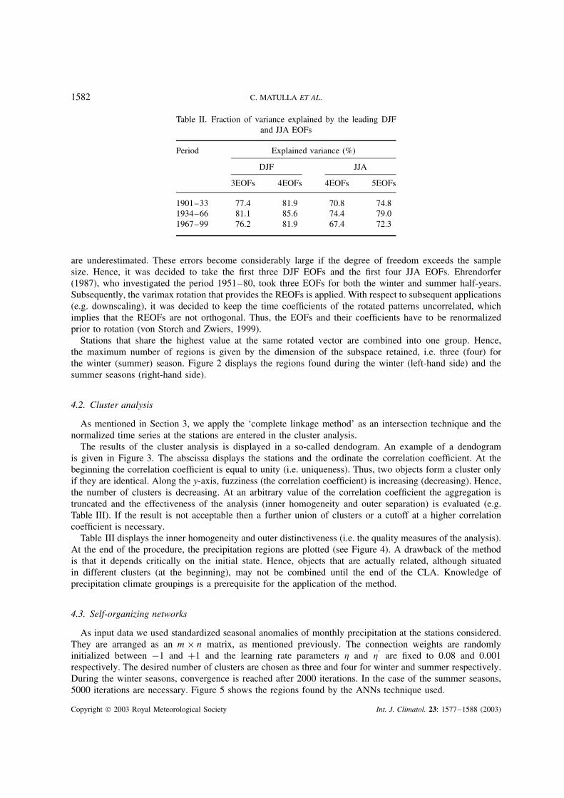
The results of the cluster analysis is displayed in a so-called dendogram. An example of a dendogramis given in Figure 3. The abscissa displays the stations and the ordinate the correlation coefficient. At thebeginning the correlation coefficient is equal to unity (i.e. uniqueness). Thus, two objects form a cluster onlyif they are identical. Along the y-axis, fuzziness (the correlation coefficient) is increasing (decreasing). Hence,the number of clusters is decreasing. At an arbitrary value of the correlation coefficient the aggregation istruncated and the effectiveness of the analysis (inner homogeneity and outer separation) is evaluated (e.g.Table III). If the result is not acceptable then a further union of clusters or a cutoff at a higher correlationcoefficient is necessary.

Table III displays the inner homogeneity and outer distinctiveness (i.e. the quality measures of the analysis).At the end of the procedure, the precipitation regions are plotted (see Figure 4). A drawback of the methodis that it depends critically on the initial state. Hence, objects that are actually related, although situatedin different clusters (at the beginning), may not be combined until the end of the CLA. Knowledge ofprecipitation climate groupings is a prerequisite for the application of the method.

4.3. Self-organizing networks

As input data we used standardized seasonal anomalies of monthly precipitation at the stations considered.They are arranged as an m × n matrix, as mentioned previously. The connection weights are randomlyinitialized between −1 and +1 and the learning rate parameters η and η

′are fixed to 0.08 and 0.001

respectively. The desired number of clusters are chosen as three and four for winter and summer respectively.During the winter seasons, convergence is reached after 2000 iterations. In the case of the summer seasons,5000 iterations are necessary. Figure 5 shows the regions found by the ANNs technique used.



DJF REOFs1901-1933

DJF REOFs1934-1966

DJF REOFs1967-1999

JJA REOFs1901-1933

JJA REOFs1934-1966

JJA REOFs1967-1999

Figure 2. Left (right): DJF (JJA) groups formed by three (four) REOFs. Shading indicates areas above 1200 m

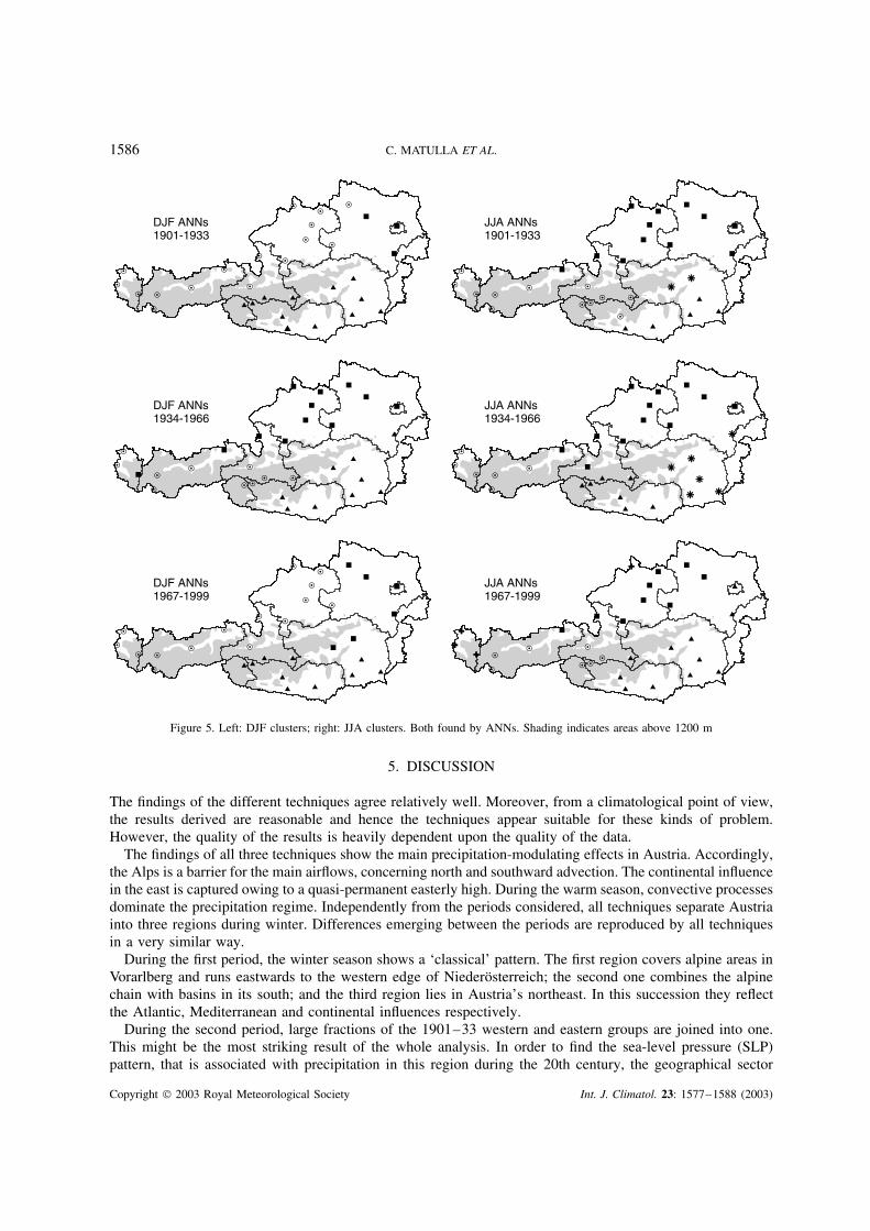
4.4. Comparative synopsis for winter

Period 1901–33: the findings of CLA and ANNs are identical. Differences in the REOFs appear onlyalong the edge between the region defined by a square (�), lying in the northeast of Austria, and the regiondefined by a circle (°), covering the territory in the north of the main alpine peaks from Vorarlberg to theMuhlviertel. The third region, defined by a triangle (�), runs along the alpine chain and includes all stationsto its south.

Period 1934–66: during this period, the results of REOFs and ANNs are strongly linked more so than tothe results of CLA. All techniques combine stations in the northern plateaus (Wein-, Wald- and Muhlviertel)with stations in and around Salzburg (�). Additionally, ANNs and REOFs show a connection to stations inVorarlberg. Unit (�) extends from stations in the vicinity of the southern basins (Grazer and Klagenfurterbasin) to the northeast. The remaining stations (°) form a group, which runs from Vorarlberg acrossTirol to the southern edge of Salzburg. Noticeable differences between the techniques appear around theHohe Tauern.

Period 1967–99: the situation is related to the first period. During this period, results of REOFs and CLAare sightly closer to each other than to findings of ANNs. However, differences occur only in the vicinity ofthe Hohe Tauern. One feature appears worth mentioning, i.e. the extension of the northeastern group (�) intoSteiermark, which is found by all methods.



1.0

0.9

0.8

0.7

0.6

0.5

0.40.30.20.10.0

-0.2

-0.4

-0.6

25272920231315 8 10121626283130 1 3 5 4 6 9 2 11 7 14182219172124

DJF 1901 -1933

' cut

off '

Figure 3. DJF dendogram for the period 1901–33

Table III. Assessment of CLA results for the winter season. Fischer and Pearson correlation coefficientsmeasure the homogeneity inside the clusters. The correlation matrix determines the similarity between

the clusters

Period Measure Cluster 1 Cluster 2 Cluster 3 No clustering

1901–33 Fischer 1.01 1.01 0.75 0.48Pearson 0.77 0.76 0.64 0.45Correlation Matrix 1.00 0.42 0.24

0.42 1.00 0.440.24 0.44 1.00

1934–66 Fischer 0.90 0.92 0.91 0.59Pearson 0.72 0.72 0.72 0.53Correlation Matrix 1.00 0.58 0.41

0.58 1.00 0.710.41 0.71 1.00

1967–99 Fischer 1.12 0.77 0.82 0.48Pearson 0.81 0.65 0.68 0.45Correlation Matrix 1.00 0.57 −0.01

0.57 1.00 0.50−0.01 0.50 1.00

During all episodes investigated, three regions can be distinguished. A rough classification might be: oneregion covers Austria’s south, another comprises the stations in the northeast and the third contains the westernparts of Austria. The agreement among the methods is satisfying. Two features appear worth mentioning: thelarge region covering the northern plateaus (�) during the second period (1934–66), and the combination ofthe northeastern part with stations in the Steiermark (1967–99) are both detected by all methods. The patternsfound in the first (1901–33) and third (1967–99) episodes share more similarities than those found in period1934–66.



DJF cluster1901-1933



JJA cluster1901-1933



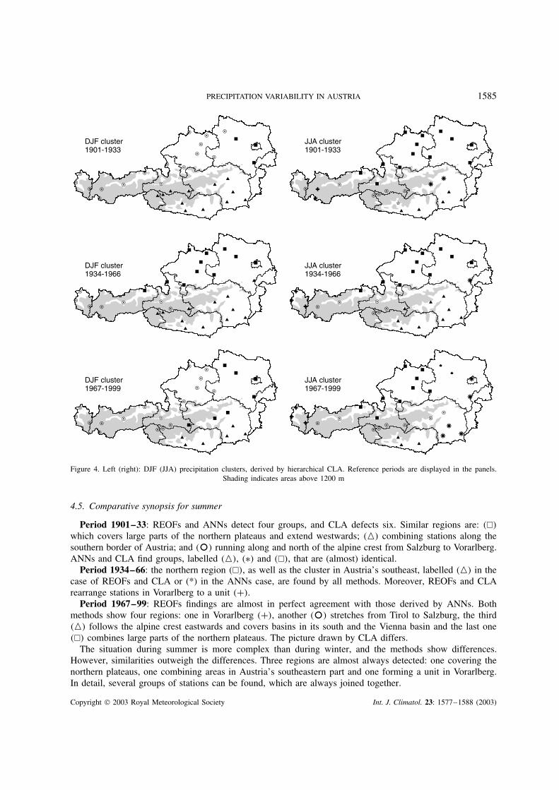
Figure 4. Left (right): DJF (JJA) precipitation clusters, derived by hierarchical CLA. Reference periods are displayed in the panels.Shading indicates areas above 1200 m

4.5. Comparative synopsis for summer

Period 1901–33: REOFs and ANNs detect four groups, and CLA defects six. Similar regions are: (�)

which covers large parts of the northern plateaus and extend westwards; (�) combining stations along thesouthern border of Austria; and (°) running along and north of the alpine crest from Salzburg to Vorarlberg.ANNs and CLA find groups, labelled (�), (∗) and (�), that are (almost) identical.

Period 1934–66: the northern region (�), as well as the cluster in Austria’s southeast, labelled (�) in thecase of REOFs and CLA or (*) in the ANNs case, are found by all methods. Moreover, REOFs and CLArearrange stations in Vorarlberg to a unit (+).

Period 1967–99: REOFs findings are almost in perfect agreement with those derived by ANNs. Bothmethods show four regions: one in Vorarlberg (+), another (°) stretches from Tirol to Salzburg, the third(�) follows the alpine crest eastwards and covers basins in its south and the Vienna basin and the last one(�) combines large parts of the northern plateaus. The picture drawn by CLA differs.

The situation during summer is more complex than during winter, and the methods show differences.However, similarities outweigh the differences. Three regions are almost always detected: one covering thenorthern plateaus, one combining areas in Austria’s southeastern part and one forming a unit in Vorarlberg.In detail, several groups of stations can be found, which are always joined together.



DJF ANNs1901-1933

DJF ANNs1934-1966

DJF ANNs1967-1999

JJA ANNs1901-1933

JJA ANNs1934-1966

JJA ANNs1967-1999

Figure 5. Left: DJF clusters; right: JJA clusters. Both found by ANNs. Shading indicates areas above 1200 m

5. DISCUSSION

The findings of the different techniques agree relatively well. Moreover, from a climatological point of view,the results derived are reasonable and hence the techniques appear suitable for these kinds of problem.However, the quality of the results is heavily dependent upon the quality of the data.

The findings of all three techniques show the main precipitation-modulating effects in Austria. Accordingly,the Alps is a barrier for the main airflows, concerning north and southward advection. The continental influencein the east is captured owing to a quasi-permanent easterly high. During the warm season, convective processesdominate the precipitation regime. Independently from the periods considered, all techniques separate Austriainto three regions during winter. Differences emerging between the periods are reproduced by all techniquesin a very similar way.

During the first period, the winter season shows a ‘classical’ pattern. The first region covers alpine areas inVorarlberg and runs eastwards to the western edge of Niederosterreich; the second one combines the alpinechain with basins in its south; and the third region lies in Austria’s northeast. In this succession they reflectthe Atlantic, Mediterranean and continental influences respectively.

During the second period, large fractions of the 1901–33 western and eastern groups are joined into one.This might be the most striking result of the whole analysis. In order to find the sea-level pressure (SLP)pattern, that is associated with precipitation in this region during the 20th century, the geographical sector



from 50 °W to 30 °E and 35 °N to 65 °N is extracted from the Northern Hemisphere SLP dataset (Trenberthand Paolino, 1980) and investigated by means of PCA and multiple linear regression. The most importantfeatures found are: (i) a negative anomaly over large parts of Europe having its minimum over Scandinavia;(ii) almost zero values south of Iceland and a poorly developed positive anomaly in the west of Spain. Thispoints to air mass advection from the northwest leading to precipitation at the northern border of the entireAlps. However, another region, more clearly influenced by the Atlantic, can be found in the central Alps.

The third period only shows a small region influenced by the Mediterranean and a larger one undercontinental influence. During this period the region influenced by the Atlantic is similar to the first period.Although Ehrendorfer (1987) uses other data, another period (1951–80) and investigates half-years, his resultsare similar to our results.

During the summer season, Austria’s precipitation pattern is more patchy. Not all regions can be easilyrelated to different air flows or precipitation regimes. Contrary to winter, only three regions are almost similarfor all techniques. The first one is located in the central Alps (Tyrolian Alps and Hohe Tauern), an area thatis known for low convective precipitation compared with other parts in Austria. The second one covers areasfrom Salzburg to the Waldviertel in the north of the Alps, and the third region is situated in the southeastof Austria. The differences between the periods are of the same magnitude as the differences produced bydifferent techniques within the periods. Thus, a comprehensive meteorological interpretation is not possible.

Taking into account the different rain-producing mechanisms, it is not surprising that precipitation duringsummer is highly variable in comparison with winter precipitation. Precipitation events during winterare mainly triggered by large-scale advective processes, with sizeable temporal extent. During summer,precipitation is dominated by local-scale short-term convective processes. These differences are responsiblefor the precipitation distribution depending on the seasonal cycle.

6. CONCLUSIONS

The techniques are able to reveal the seasonal dependence of Austria’s precipitation patterns. Differencesamong the methods are larger during summer than during winter. In the case of CLA the differences betweensummer and winter can be seen directly in the dendrograms. During summer, it is difficult to distinguishclearly between different groups, and this leads to a reduced outer separation and inner homogeneity of thefinal regions. In the case of REOFs, the dimension of the subspace, required to comprise approximately thesame fraction of variance as in winter, is higher. Hence, the corresponding patterns are likely to be morecomplicated than in winter. In the case of ANNs, during winter, only one choice of parameters was sufficientfor all episodes. During summer, these parameters had to be adjusted for each period separately. Hence,differences between the methods are more pronounced in summer than in winter.

To summarize, the results found by the different techniques are in agreement. This is particularly true forthe winter season, but even during summer there are common features. This fact inspires confidence in theusefulness of the methods.

CLA, REOFs and ANNs depend on the objective of the research: CLA offers many possibilities ofquantifying similarity, i.e. to measure how two stations are alike and how they differ; REOFs depend onthe number of EOFs retained and the rotation method, and in ANNs several parameters (e.g. learning rates,distance weighting, etc.) can be adjusted.

The results of this work are now being used in downscaling studies. For every region a single downscalingmodel is established (Woth, 2001), to infer information from larger to smaller scales. Further goals might bethe application of the techniques presented to: (i) larger amounts of station data, which generally compriseonly a short period in comparison with the total period available in this work; (ii) larger regions, e.g. thewhole alpine area; and (iii) detection of homogeneous regions with respect to time.

ACKNOWLEDGEMENTS

This study was conducted within the research project ‘Usability of different downscaling methods in complexterrain’ funded by the Austrian Federal Ministry of Education, Science and Culture. The Zentralanstalt fur



Meteorologie und Geodynamik provided the ALOCLIM dataset. We would like to thank H. Matulla, S.Wagner and D. Bray for fruitful discussions and for helping us with the manuscript, and H. Kuhn for hissupport in providing and maintaining computer facilities. The manuscript was improved by the comments oftwo anonymous reviewers.

REFERENCES

Auer I. 1993. Niederschlagsschwankungen in Osterreich. Osterreichische Beitrage zu Meteorologie und Geophysik 7: 73 pp.Auer I, Bohm R, Schoner W. 2001. Austrian long-term climate 1767–2000. Osterreichische Beitrage zu Meteorologie und Geophysik

25: 147 pp.Bohm R, Auer I, Brunetti M, Maugeri M, Nanni T, Schoner W. 2001. Regional temperature variability in the European Alps:

1760–1998 from homogenized instrumental time series. International Journal of Climatology 21: 1779–1801.Ehrendorfer M. 1987. A regionalization of Austria’s precipitation climate using principal component analysis. Journal of Climatology

7: 71–89.Foody GM. 1999. Applications of the self-organising feature map neural network in community data analysis. Ecological Modelling

120: 97–107.Haykin S. 1994. Neural Networks: A Comprehensive Foundation. MacMillan College Publishing Company.Hewitson BC, Crane RG. 2002. Self-organizing mags: applications to synoptic climatology. Climate Research 22: 13–26.Jackson IJ, Weinand H. 1994. Towards a classification of tropical rainfall stations. International Journal of Climatology 14: 263–286.Lexer MJ, Honninger K, Scheifinger H, Matulla C, Groll N, Kromp-Kolb H, Schaudauer K, Starlinger F, Englisch M. 2002. The

sensitivity of Austrian forests to scenarios of climate change: a large-scale risk assessment based on a modified gap model andforest inventory data. Forest Ecology and Management 162: 53–72.

Michaelides SC, Pattichis CS, Kleovoulou G. 2001. Classification of rainfall variability by using artificial neural networks. InternationalJournal of Climatology 21: 1401–1414.

Preisendorfer RW. 1988. Principal Component Analysis in Meteorology and Oceanography. Elsevier: Seattle.Ramos MC. 2001. Divisive and hierarchical clustering techniques to analyse variability of rainfall distribution patterns in a Mediterranean

region. Atmospheric Research 57: 123–138.Richman MB. 1986. Rotation of principal components. International Journal of Climatology 6: 293–335.Rumelhart DE, Zipser D. 1985. Feature discovery by competitive learning. Cognitive Science 9: 75–112.Schwab M, Daly C, Frei C, Schar C. 2001. Hydrologischer Atlas der Schweiz. Geographisches Institut der Universitat Bern-Hydrologie,

Bundesamt fur Landestopographie: Wabern-Bern.Trenberth KE, Paolino Jr DA. 1980. The Northern Hemisphere sea-level pressure data set: trends, errors and discontinuities. Monthly

Weather Review 108: 855–872.Von Storch H, Hannoschock G. 1985. Statistical aspects of estimated principal vectors (EOFs) based on small sample sizes. Journal of

Climate and Applied Meteorology 24: 716–724.Von Storch H, Zwiers F. 1999. Statistical Analysis in Climate Research. Cambridge University Press.Widmann ML. 1996. Mesoscale variability and long-term trends of Alpine precipitation and their relation to the synoptic-scale flow.

PhD thesis, ETH Zurich.WMO (ed.). 1992. International meteorological vocabulary, Volume WMO/OMN/BMO-No.182. Secretariat of the World Meteorological

Organization.Woth K. 2001. Abschatzung einer zukunftigen Niederschlagsentwicklung mit statistischen Methoden unter Einbezug raumlicher

Differenzierungsverfahren am Beispiel des sudwesteuropaischen Raums. Master’s thesis, GKSS-Report 2001/28, University of Trier.


Documents

COMPARATIVE ANALYSIS OF SPATIAL AND · PDF file · 2006-07-26CHRISTOPH MATULLA,a,b,* EDOUARD K. PENLAP,a,c PATRICK HAASb and ... e-mail: matulla@ ... detection of climatic ﬂuctuations;