Spatial Statistics: Regression - MIT OpenCourseWare · Spatial Statistics: Regression. ... (not a file in the folder) ... Is there potential redundancy among variables based on the

1 Jennie Murack, MIT Libraries, 2015

Spatial Statistics: Regression

Part 1: Running a Regression in ArcMap and Geoda

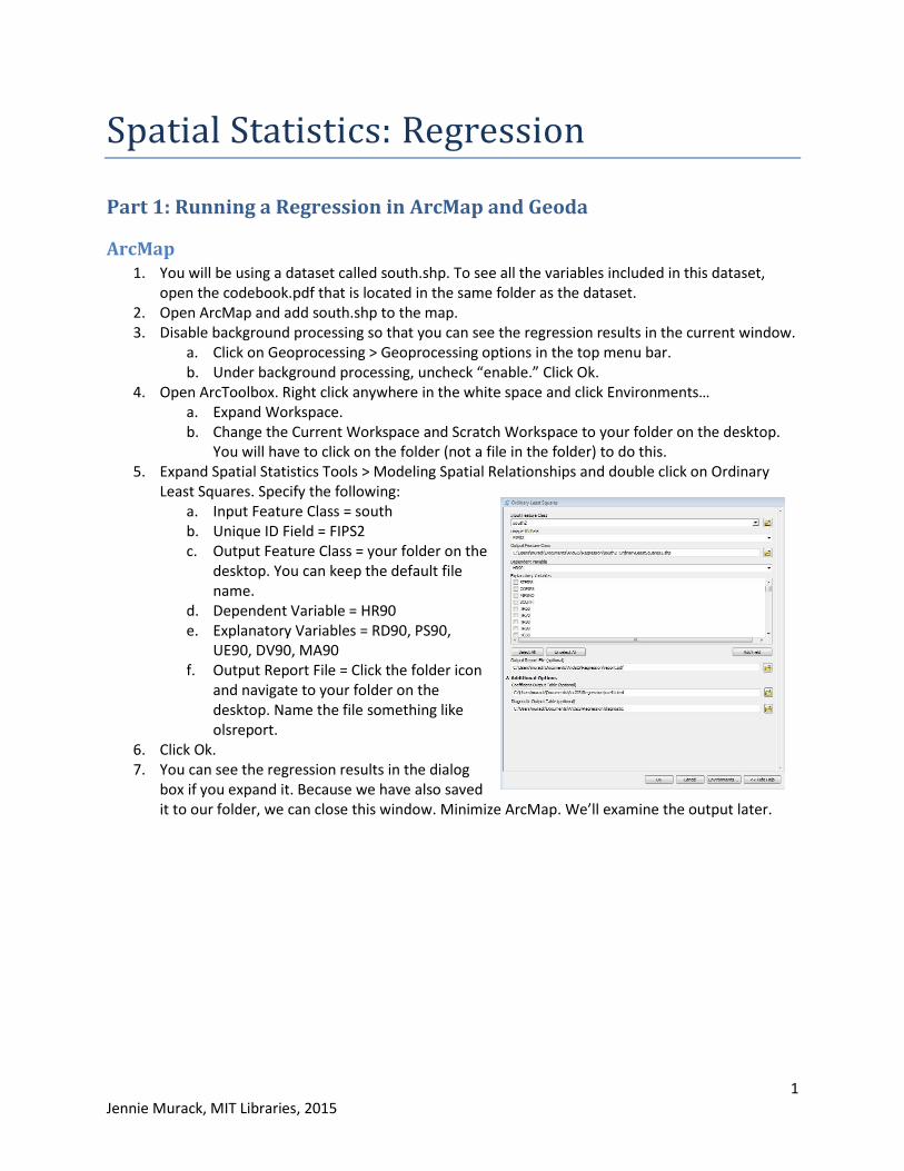
ArcMap 1. You will be using a dataset called south.shp. To see all the variables included in this dataset,

open the codebook.pdf that is located in the same folder as the dataset. 2. Open ArcMap and add south.shp to the map. 3. Disable background processing so that you can see the regression results in the current window.

a. Click on Geoprocessing > Geoprocessing options in the top menu bar. b. Under background processing, uncheck “enable.” Click Ok.

4. Open ArcToolbox. Right click anywhere in the white space and click Environments… a. Expand Workspace. b. Change the Current Workspace and Scratch Workspace to your folder on the desktop.

You will have to click on the folder (not a file in the folder) to do this. 5. Expand Spatial Statistics Tools > Modeling Spatial Relationships and double click on Ordinary

Least Squares. Specify the following: a. Input Feature Class = south b. Unique ID Field = FIPS2 c. Output Feature Class = your folder on the

desktop. You can keep the default file name.

d. Dependent Variable = HR90 e. Explanatory Variables = RD90, PS90,

UE90, DV90, MA90 f. Output Report File = Click the folder icon

and navigate to your folder on the desktop. Name the file something like olsreport.

6. Click Ok. 7. You can see the regression results in the dialog

box if you expand it. Because we have also saved it to our folder, we can close this window. Minimize ArcMap. We’ll examine the output later.


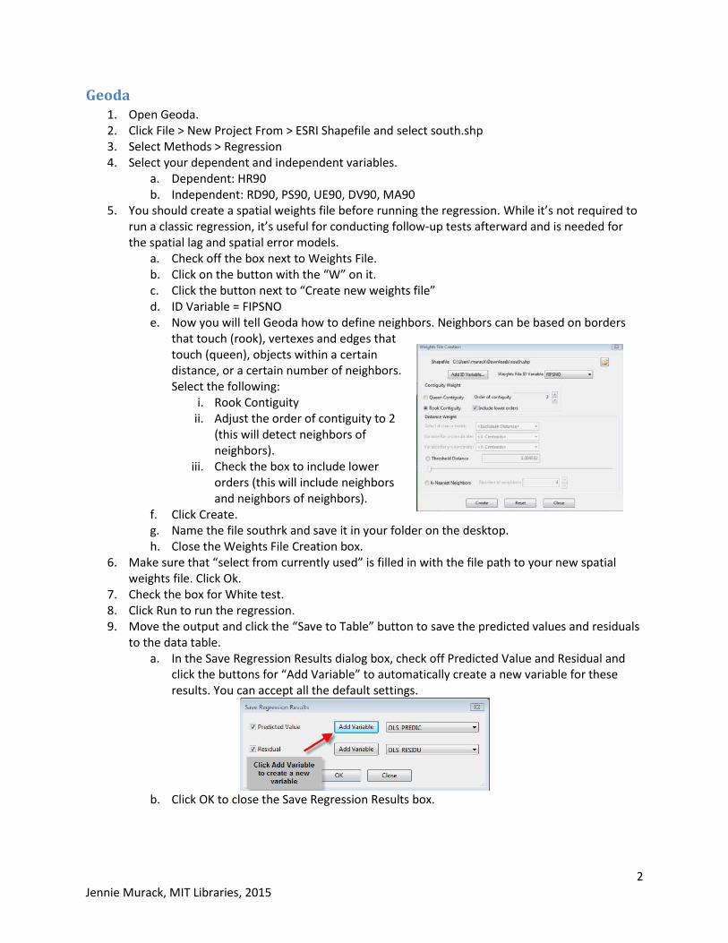
Geoda 1. Open Geoda. 2. Click File > New Project From > ESRI Shapefile and select south.shp 3. Select Methods > Regression 4. Select your dependent and independent variables.

a. Dependent: HR90 b. Independent: RD90, PS90, UE90, DV90, MA90

5. You should create a spatial weights file before running the regression. While it’s not required to run a classic regression, it’s useful for conducting follow-up tests afterward and is needed for the spatial lag and spatial error models.

a. Check off the box next to Weights File. b. Click on the button with the “W” on it. c. Click the button next to “Create new weights file” d. ID Variable = FIPSNO e. Now you will tell Geoda how to define neighbors. Neighbors can be based on borders

that touch (rook), vertexes and edges that touch (queen), objects within a certain distance, or a certain number of neighbors. Select the following:

i. Rook Contiguity ii. Adjust the order of contiguity to 2

(this will detect neighbors of neighbors).

iii. Check the box to include lower orders (this will include neighbors and neighbors of neighbors).

f. Click Create. g. Name the file southrk and save it in your folder on the desktop. h. Close the Weights File Creation box.

6. Make sure that “select from currently used” is filled in with the file path to your new spatial weights file. Click Ok.

7. Check the box for White test. 8. Click Run to run the regression. 9. Move the output and click the “Save to Table” button to save the predicted values and residuals

to the data table. a. In the Save Regression Results dialog box, check off Predicted Value and Residual and

click the buttons for “Add Variable” to automatically create a new variable for these results. You can accept all the default settings.

b. Click OK to close the Save Regression Results box.


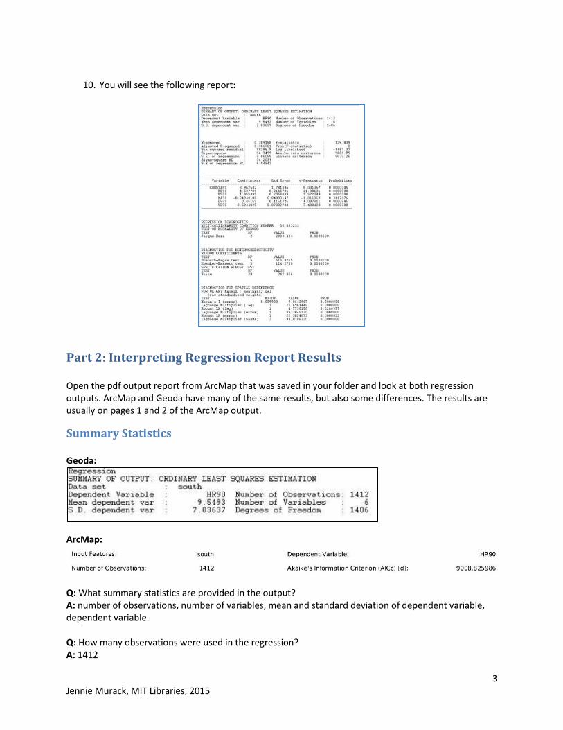
10. You will see the following report:

Part 2: Interpreting Regression Report Results Open the pdf output report from ArcMap that was saved in your folder and look at both regression outputs. ArcMap and Geoda have many of the same results, but also some differences. The results are usually on pages 1 and 2 of the ArcMap output.

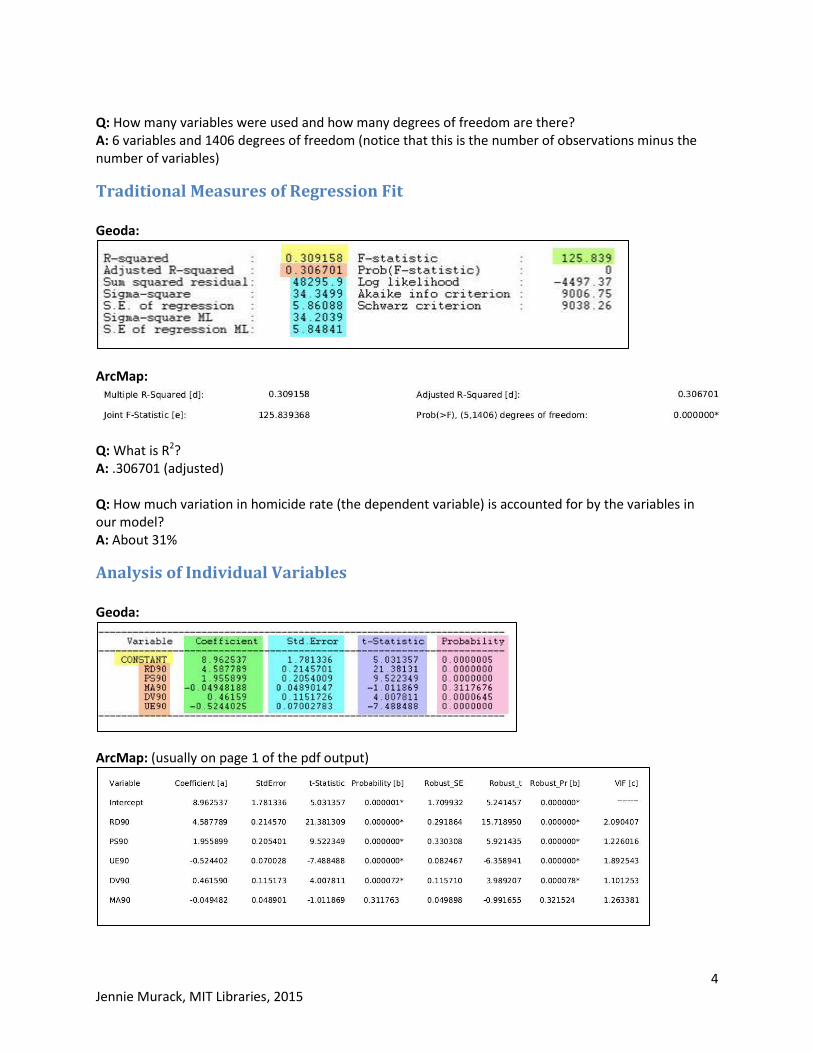
Summary Statistics Geoda:

ArcMap:

Q: What summary statistics are provided in the output? A: number of observations, number of variables, mean and standard deviation of dependent variable, dependent variable. Q: How many observations were used in the regression? A: 1412


Q: How many variables were used and how many degrees of freedom are there? A: 6 variables and 1406 degrees of freedom (notice that this is the number of observations minus the number of variables)

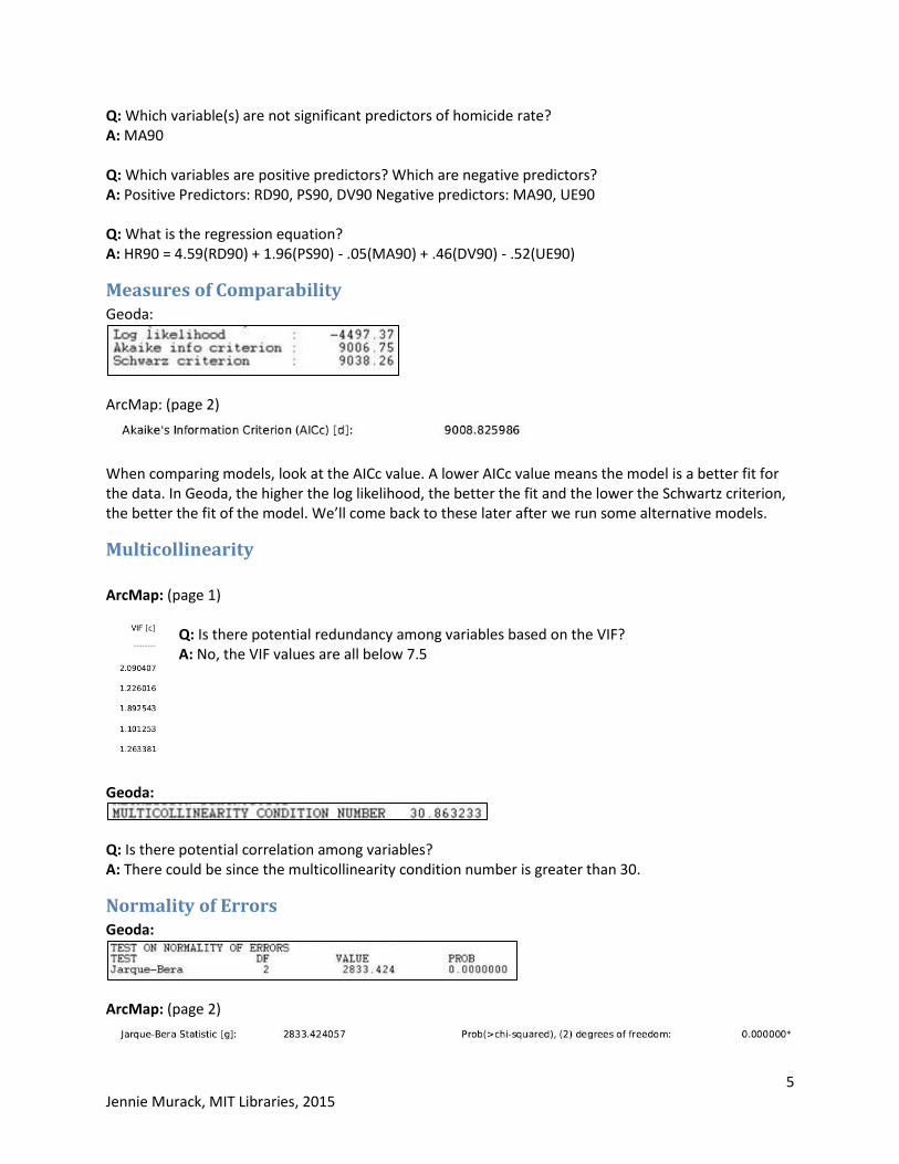
Traditional Measures of Regression Fit Geoda:

ArcMap:

Q: What is R2? A: .306701 (adjusted) Q: How much variation in homicide rate (the dependent variable) is accounted for by the variables in our model? A: About 31%

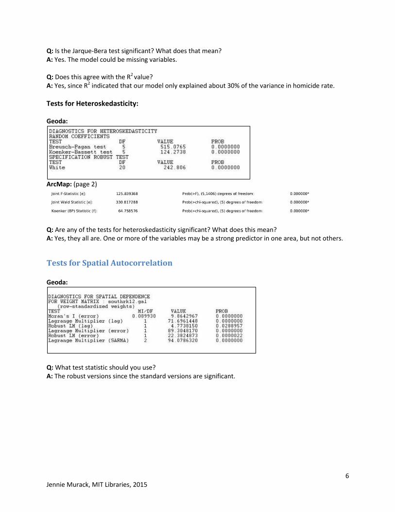
Analysis of Individual Variables Geoda:

ArcMap: (usually on page 1 of the pdf output)


Q: Which variable(s) are not significant predictors of homicide rate? A: MA90 Q: Which variables are positive predictors? Which are negative predictors? A: Positive Predictors: RD90, PS90, DV90 Negative predictors: MA90, UE90 Q: What is the regression equation? A: HR90 = 4.59(RD90) + 1.96(PS90) - .05(MA90) + .46(DV90) - .52(UE90)

Measures of Comparability Geoda:

ArcMap: (page 2)

When comparing models, look at the AICc value. A lower AICc value means the model is a better fit for the data. In Geoda, the higher the log likelihood, the better the fit and the lower the Schwartz criterion, the better the fit of the model. We’ll come back to these later after we run some alternative models.

Multicollinearity

ArcMap: (page 1)

Q: Is there potential redundancy among variables based on the VIF? A: No, the VIF values are all below 7.5

Geoda:

Q: Is there potential correlation among variables? A: There could be since the multicollinearity condition number is greater than 30.

Normality of Errors Geoda:

ArcMap: (page 2)


Q: Is the Jarque-Bera test significant? What does that mean? A: Yes. The model could be missing variables. Q: Does this agree with the R2 value? A: Yes, since R2 indicated that our model only explained about 30% of the variance in homicide rate.

Tests for Heteroskedasticity:

Geoda:

ArcMap: (page 2)

Q: Are any of the tests for heteroskedasticity significant? What does this mean? A: Yes, they all are. One or more of the variables may be a strong predictor in one area, but not others.

Tests for Spatial Autocorrelation Geoda:

Q: What test statistic should you use? A: The robust versions since the standard versions are significant.


Part 3: Fun with Residuals

Mapping Residuals Now you will map the residuals in both ArcMap and Geoda. You should get similar results in each.

ArcMap

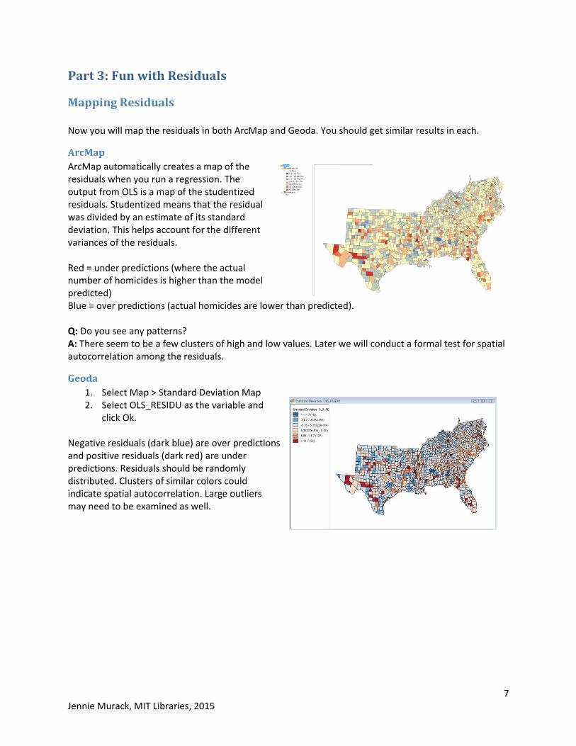
ArcMap automatically creates a map of the residuals when you run a regression. The output from OLS is a map of the studentized residuals. Studentized means that the residual was divided by an estimate of its standard deviation. This helps account for the different variances of the residuals. Red = under predictions (where the actual number of homicides is higher than the model predicted) Blue = over predictions (actual homicides are lower than predicted). Q: Do you see any patterns? A: There seem to be a few clusters of high and low values. Later we will conduct a formal test for spatial autocorrelation among the residuals.

Geoda

1. Select Map > Standard Deviation Map 2. Select OLS_RESIDU as the variable and

click Ok.

Negative residuals (dark blue) are over predictions and positive residuals (dark red) are under predictions. Residuals should be randomly distributed. Clusters of similar colors could indicate spatial autocorrelation. Large outliers may need to be examined as well.


Plotting Residuals Plotting the residual vs. one of the unique ID variables helps you identify patterns in your residuals and see unusually large residuals.

ArcMap

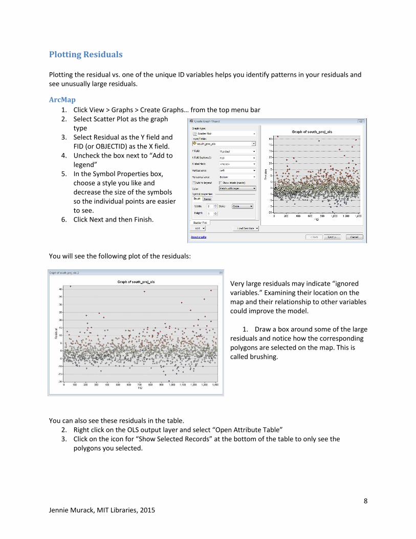
1. Click View > Graphs > Create Graphs… from the top menu bar 2. Select Scatter Plot as the graph

type 3. Select Residual as the Y field and

FID (or OBJECTID) as the X field. 4. Uncheck the box next to “Add to

legend” 5. In the Symbol Properties box,

choose a style you like and decrease the size of the symbols so the individual points are easier to see.

6. Click Next and then Finish. You will see the following plot of the residuals:

Very large residuals may indicate “ignored variables.” Examining their location on the map and their relationship to other variables could improve the model.

1. Draw a box around some of the large residuals and notice how the corresponding polygons are selected on the map. This is called brushing.

You can also see these residuals in the table.

2. Right click on the OLS output layer and select “Open Attribute Table” 3. Click on the icon for “Show Selected Records” at the bottom of the table to only see the

polygons you selected.


Geoda

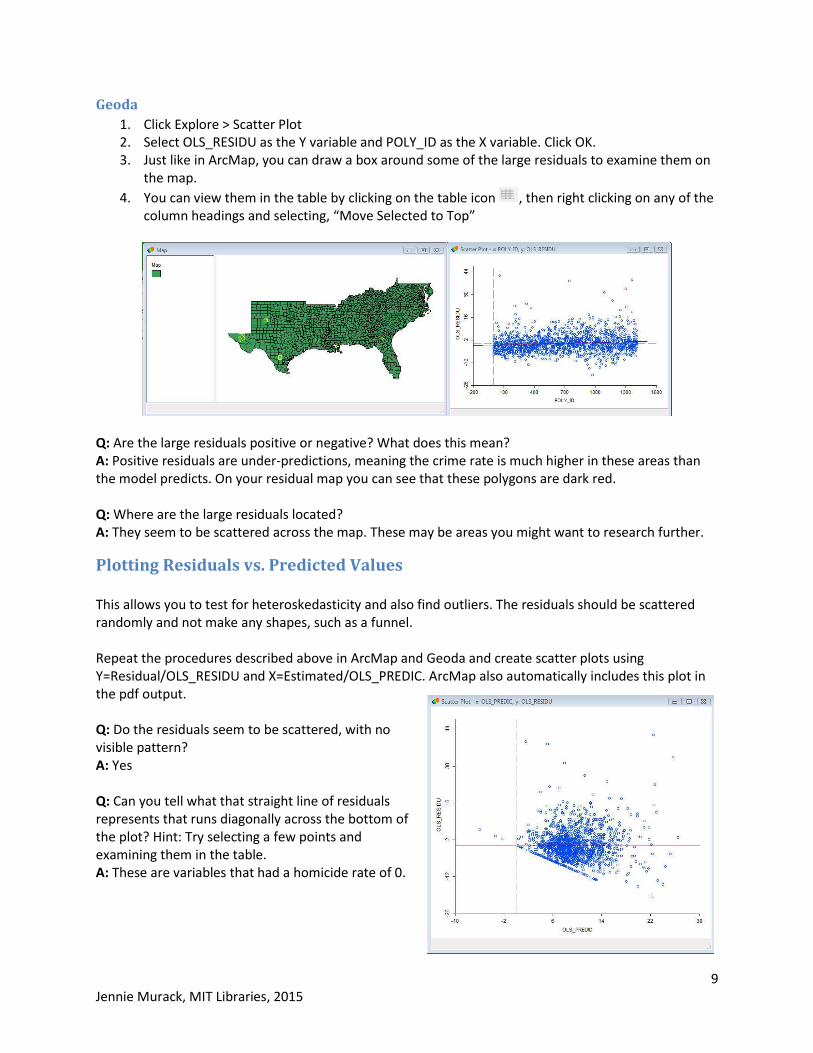
1. Click Explore > Scatter Plot 2. Select OLS_RESIDU as the Y variable and POLY_ID as the X variable. Click OK. 3. Just like in ArcMap, you can draw a box around some of the large residuals to examine them on

the map.

4. You can view them in the table by clicking on the table icon , then right clicking on any of the column headings and selecting, “Move Selected to Top”

Q: Are the large residuals positive or negative? What does this mean? A: Positive residuals are under-predictions, meaning the crime rate is much higher in these areas than the model predicts. On your residual map you can see that these polygons are dark red. Q: Where are the large residuals located? A: They seem to be scattered across the map. These may be areas you might want to research further.

Plotting Residuals vs. Predicted Values This allows you to test for heteroskedasticity and also find outliers. The residuals should be scattered randomly and not make any shapes, such as a funnel. Repeat the procedures described above in ArcMap and Geoda and create scatter plots using Y=Residual/OLS_RESIDU and X=Estimated/OLS_PREDIC. ArcMap also automatically includes this plot in the pdf output. Q: Do the residuals seem to be scattered, with no visible pattern? A: Yes Q: Can you tell what that straight line of residuals represents that runs diagonally across the bottom of the plot? Hint: Try selecting a few points and examining them in the table. A: These are variables that had a homicide rate of 0.


Testing Residuals for Spatial Autocorrelation

ArcMap

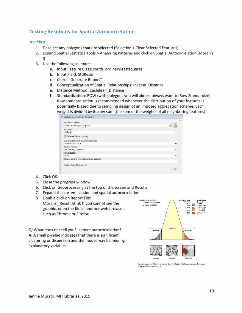
1. Deselect any polygons that are selected (Selection > Clear Selected Features) 2. Expand Spatial Statistics Tools > Analyzing Patterns and click on Spatial Autocorrelation (Moran’s

I) 3. Use the following as inputs:

a. Input Feature Class: south_ordinaryleastsquares b. Input Field: StdResid c. Check “Generate Report” d. Conceptualization of Spatial Relationships: Inverse_Distance e. Distance Method: Euclidean_Distance f. Standardization: ROW (with polygons you will almost always want to Row Standardize)

Row standardization is recommended whenever the distribution of your features is potentially biased due to sampling design of an imposed aggregation scheme. Each weight is divided by its row sum (the sum of the weights of all neighboring features).

4. Click OK 5. Close the progress window. 6. Click on Geoprocessing at the top of the screen and Results. 7. Expand the current session and spatial autocorrelation 8. Double click on Report File:

MoransI_Result.html. If you cannot see the graphic, open the file in another web browser, such as Chrome or Firefox.

Q: What does this tell you? Is there autocorrelation? A: A small p-value indicates that there is significant clustering or dispersion and the model may be missing explanatory variables.


Geoda

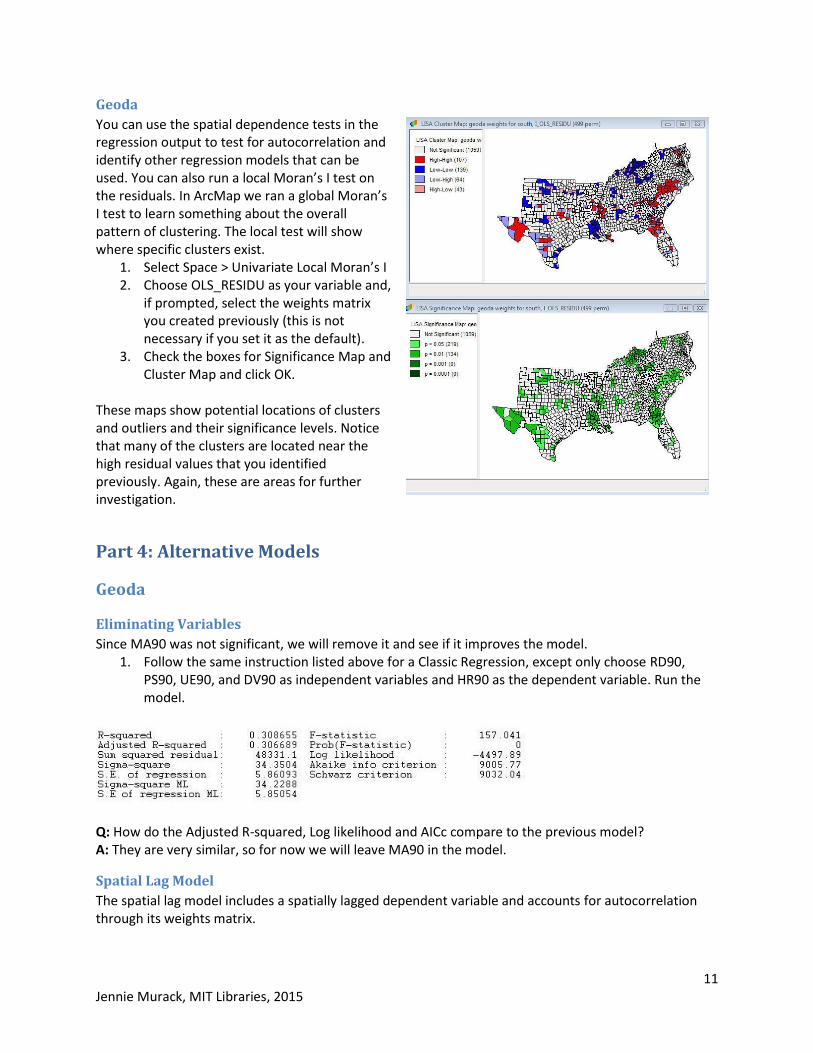
You can use the spatial dependence tests in the regression output to test for autocorrelation and identify other regression models that can be used. You can also run a local Moran’s I test on the residuals. In ArcMap we ran a global Moran’s I test to learn something about the overall pattern of clustering. The local test will show where specific clusters exist.

1. Select Space > Univariate Local Moran’s I 2. Choose OLS_RESIDU as your variable and,

if prompted, select the weights matrix you created previously (this is not necessary if you set it as the default).

3. Check the boxes for Significance Map and Cluster Map and click OK.

These maps show potential locations of clusters and outliers and their significance levels. Notice that many of the clusters are located near the high residual values that you identified previously. Again, these are areas for further investigation.

Part 4: Alternative Models

Geoda

Eliminating Variables

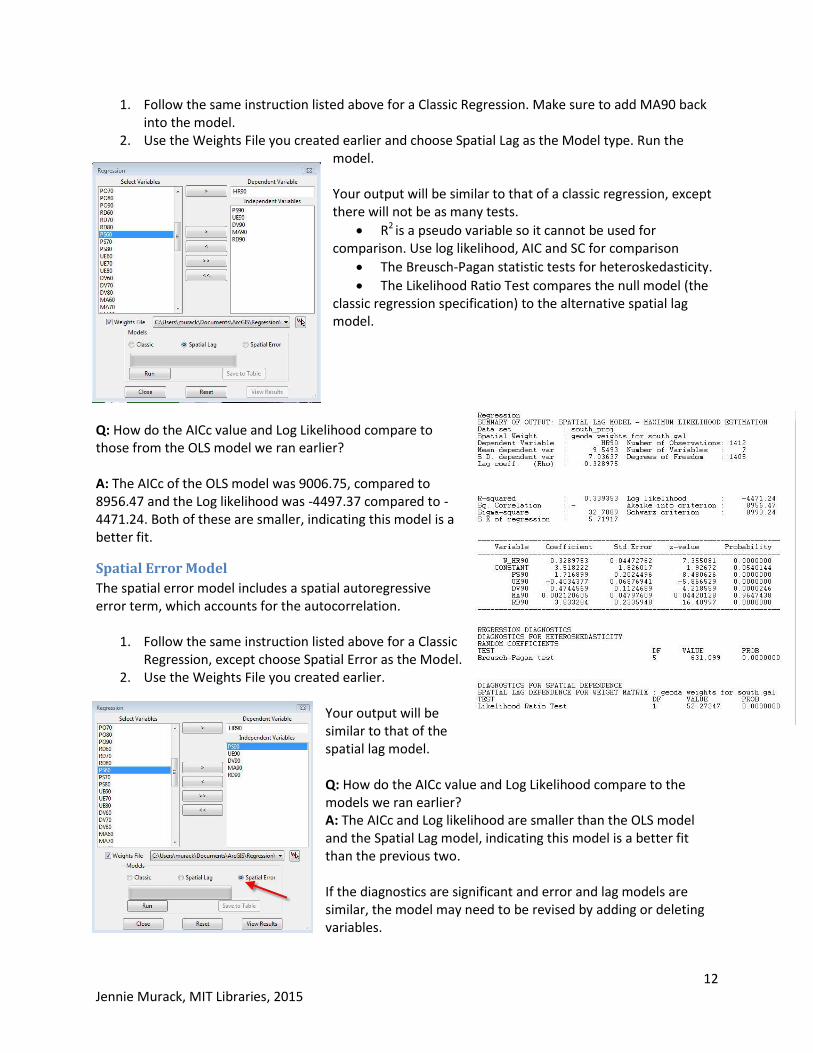
Since MA90 was not significant, we will remove it and see if it improves the model. 1. Follow the same instruction listed above for a Classic Regression, except only choose RD90,

PS90, UE90, and DV90 as independent variables and HR90 as the dependent variable. Run the model.

Q: How do the Adjusted R-squared, Log likelihood and AICc compare to the previous model? A: They are very similar, so for now we will leave MA90 in the model.

Spatial Lag Model

The spatial lag model includes a spatially lagged dependent variable and accounts for autocorrelation through its weights matrix.


1. Follow the same instruction listed above for a Classic Regression. Make sure to add MA90 back into the model.

2. Use the Weights File you created earlier and choose Spatial Lag as the Model type. Run the model.

Your output will be similar to that of a classic regression, except there will not be as many tests.

R2 is a pseudo variable so it cannot be used for comparison. Use log likelihood, AIC and SC for comparison

The Breusch-Pagan statistic tests for heteroskedasticity.

The Likelihood Ratio Test compares the null model (the classic regression specification) to the alternative spatial lag model.

Q: How do the AICc value and Log Likelihood compare to those from the OLS model we ran earlier? A: The AICc of the OLS model was 9006.75, compared to 8956.47 and the Log likelihood was -4497.37 compared to -4471.24. Both of these are smaller, indicating this model is a better fit.

Spatial Error Model

The spatial error model includes a spatial autoregressive error term, which accounts for the autocorrelation.

1. Follow the same instruction listed above for a Classic Regression, except choose Spatial Error as the Model.

2. Use the Weights File you created earlier. Your output will be similar to that of the spatial lag model. Q: How do the AICc value and Log Likelihood compare to the models we ran earlier? A: The AICc and Log likelihood are smaller than the OLS model and the Spatial Lag model, indicating this model is a better fit than the previous two. If the diagnostics are significant and error and lag models are similar, the model may need to be revised by adding or deleting variables.


ArcMap

Geographically Weighted Regression

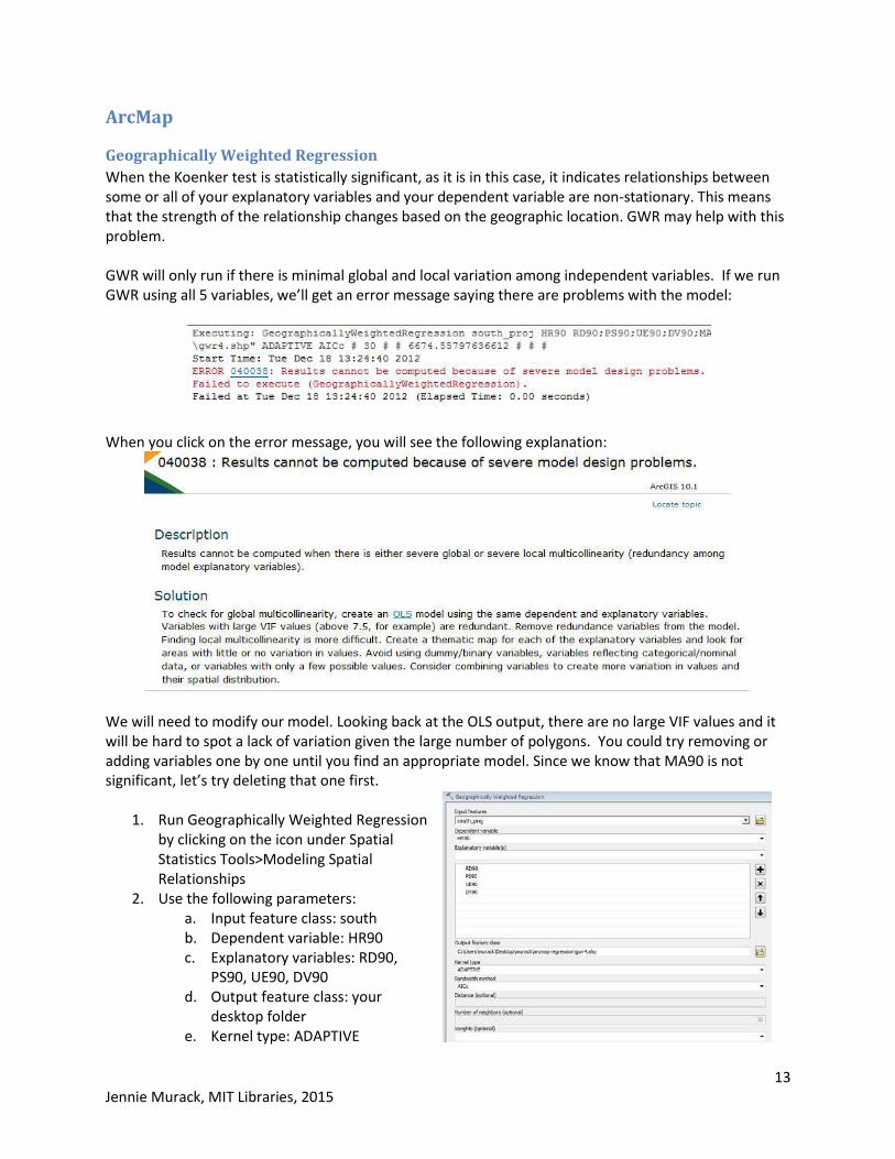
When the Koenker test is statistically significant, as it is in this case, it indicates relationships between some or all of your explanatory variables and your dependent variable are non-stationary. This means that the strength of the relationship changes based on the geographic location. GWR may help with this problem. GWR will only run if there is minimal global and local variation among independent variables. If we run GWR using all 5 variables, we’ll get an error message saying there are problems with the model:

When you click on the error message, you will see the following explanation:

We will need to modify our model. Looking back at the OLS output, there are no large VIF values and it will be hard to spot a lack of variation given the large number of polygons. You could try removing or adding variables one by one until you find an appropriate model. Since we know that MA90 is not significant, let’s try deleting that one first.

1. Run Geographically Weighted Regression by clicking on the icon under Spatial Statistics Tools>Modeling Spatial Relationships

2. Use the following parameters: a. Input feature class: south b. Dependent variable: HR90 c. Explanatory variables: RD90,

PS90, UE90, DV90 d. Output feature class: your

desktop folder e. Kernel type: ADAPTIVE


f. Bandwidth method: AICc (you will let the tool find the optimal number of neighbors)

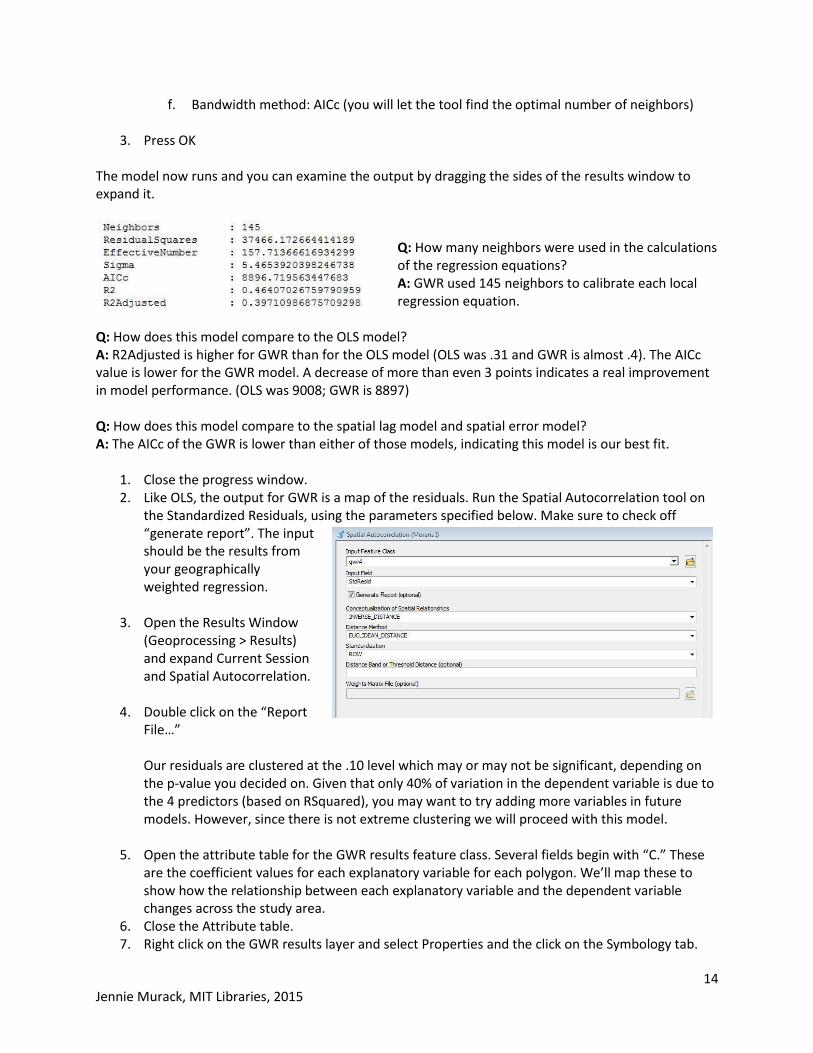
3. Press OK The model now runs and you can examine the output by dragging the sides of the results window to expand it.

Q: How many neighbors were used in the calculations of the regression equations? A: GWR used 145 neighbors to calibrate each local regression equation.

Q: How does this model compare to the OLS model? A: R2Adjusted is higher for GWR than for the OLS model (OLS was .31 and GWR is almost .4). The AICc value is lower for the GWR model. A decrease of more than even 3 points indicates a real improvement in model performance. (OLS was 9008; GWR is 8897) Q: How does this model compare to the spatial lag model and spatial error model? A: The AICc of the GWR is lower than either of those models, indicating this model is our best fit.

1. Close the progress window. 2. Like OLS, the output for GWR is a map of the residuals. Run the Spatial Autocorrelation tool on

the Standardized Residuals, using the parameters specified below. Make sure to check off “generate report”. The input should be the results from your geographically weighted regression.

3. Open the Results Window

(Geoprocessing > Results) and expand Current Session and Spatial Autocorrelation.

4. Double click on the “Report File…” Our residuals are clustered at the .10 level which may or may not be significant, depending on the p-value you decided on. Given that only 40% of variation in the dependent variable is due to the 4 predictors (based on RSquared), you may want to try adding more variables in future models. However, since there is not extreme clustering we will proceed with this model.

5. Open the attribute table for the GWR results feature class. Several fields begin with “C.” These are the coefficient values for each explanatory variable for each polygon. We’ll map these to show how the relationship between each explanatory variable and the dependent variable changes across the study area.

6. Close the Attribute table. 7. Right click on the GWR results layer and select Properties and the click on the Symbology tab.


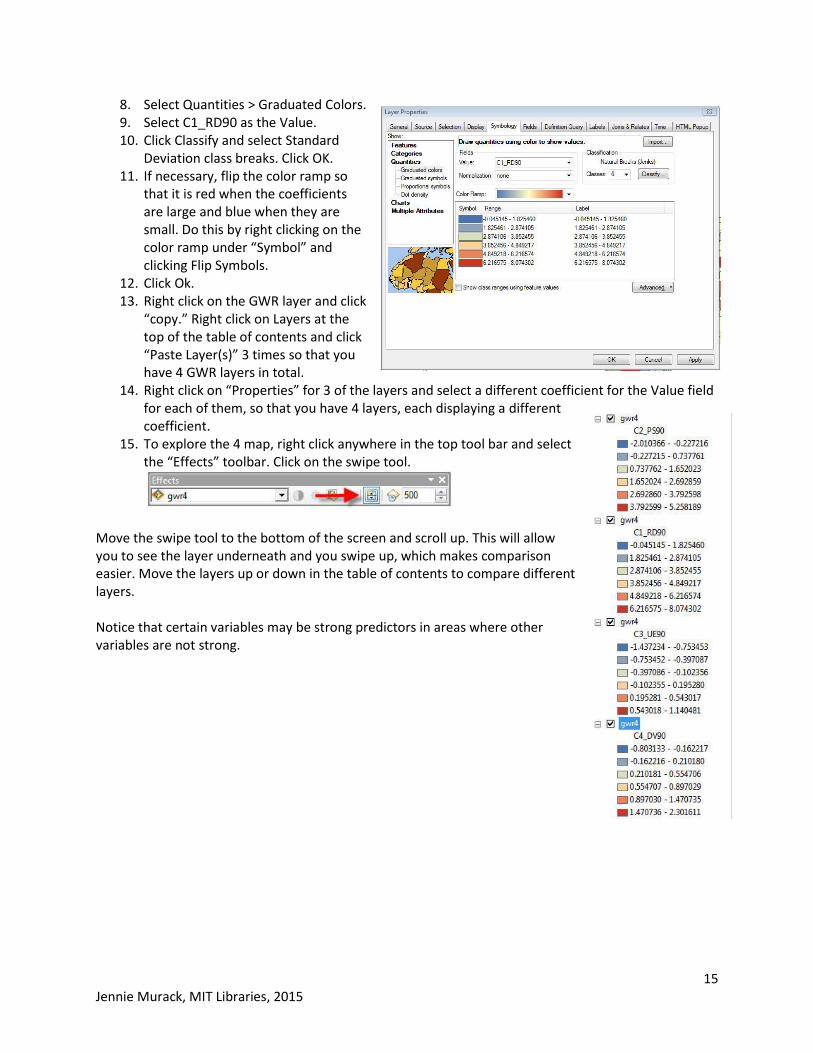
8. Select Quantities > Graduated Colors. 9. Select C1_RD90 as the Value. 10. Click Classify and select Standard

Deviation class breaks. Click OK. 11. If necessary, flip the color ramp so

that it is red when the coefficients are large and blue when they are small. Do this by right clicking on the color ramp under “Symbol” and clicking Flip Symbols.

12. Click Ok. 13. Right click on the GWR layer and click

“copy.” Right click on Layers at the top of the table of contents and click “Paste Layer(s)” 3 times so that you have 4 GWR layers in total.

14. Right click on “Properties” for 3 of the layers and select a different coefficient for the Value field for each of them, so that you have 4 layers, each displaying a different coefficient.

15. To explore the 4 map, right click anywhere in the top tool bar and select the “Effects” toolbar. Click on the swipe tool.

Move the swipe tool to the bottom of the screen and scroll up. This will allow you to see the layer underneath and you swipe up, which makes comparison easier. Move the layers up or down in the table of contents to compare different layers. Notice that certain variables may be strong predictors in areas where other variables are not strong.

MIT OpenCourseWarehttp://ocw.mit.edu

RES.STR-001 Geographic Information System (GIS)TutorialJanuary IAP 2016

For information about citing these materials or our Terms of Use, visit: http://ocw.mit.edu/terms.

http://ocw.mit.edu/terms

http://ocw.mit.edu

Documents

Spatial Statistics: Regression - MIT OpenCourseWare · Spatial Statistics: Regression. ... (not a file in the folder) ... Is there potential redundancy among variables based on the