Available online at www.sciencedirect.com

) 34–48www.elsevier.com/locate/catena

Catena 73 (2008

Spatial patterns of ecohydrologic properties on a hillslope-alluvialfan transect, central New Mexico

David R. Bedford a,b,⁎, Eric E. Small b,1

a U.S. Geological Survey, 345 Middlefield Rd MS-973, Menlo Park, CA 94025, USAb Department of Geological Sciences, University of Colorado, Boulder, CO 80309, USA

Received 24 May 2007; received in revised form 25 August 2007; accepted 31 August 2007

Abstract

Spatial patterns of soil properties are linked to patchy vegetation in arid and semi-arid landscapes. The patterns of soil properties are generallyassumed to be linked to the ecohydrological functioning of patchy dryland vegetation ecosystems. We studied the effects of vegetation canopy, itsspatial pattern, and landforms on soil properties affecting overland flow and infiltration in shrublands at the Sevilleta National Wildlife Refuge/LTER in central New Mexico, USA. We studied the patterns of microtopography and saturated conductivity (Ksat), and generally found it to beaffected by vegetation canopy and pattern, as well as landform type. On gently sloping alluvial fans, both microtopography and Ksat are highunder vegetation canopy and decay with distance from plant center. On steeper hillslope landforms, only microtopography was significantly higherunder vegetation canopy, while there was no significant difference in Ksat between vegetation and interspaces. Using geostatistics, we found thatthe spatial pattern of soil properties was determined by the spatial pattern of vegetation. Most importantly, the effects of vegetation were present inthe unvegetated interspaces 2–4 times the extent of vegetation canopy, on the order of 2–3 m. Our results have implications for the understandingthe ecohydrologic function of semi-arid ecosystems as well as the parameterization of hydrologic models.© 2007 Elsevier B.V. All rights reserved.

Keywords: Spatial patterns; Ecohydrology; Alluvial fans; Bajada; Hillslope; Vegetation; Soil properties

1. Introduction

The primary tenet of arid land ecology is that organisms mustconcentrate and conserve resources such as water, nutrients, andsoil, typically in response to resource pulses (e.g. Ludwig andTongway, 1995; Noy-Meir, 1973; Schwinning and Sala, 2004).One of the mechanisms attributed to resource concentration isthe redistribution of resources linked to patchy vegetation andheterogeneous soil properties (Bergkamp et al., 1996; Bre-shears, 2006; Breshears et al., 1998; Ludwig et al., 2005;Sanchez and Puigdefabregas, 1994). Many studies have shownthat the physical and chemical properties exhibiting heteroge-

⁎ Corresponding author. U.S. Geological Survey, 345 Middlefield Rd MS-973, Menlo Park, CA 94025, USA. Fax: +1 303 492 2606.

E-mail addresses: dbedford@usgs.gov (D.R. Bedford),eric.small@colorado.edu (E.E. Small).1 Fax: +1 303 492 2606.

0341-8162/$ - see front matter © 2007 Elsevier B.V. All rights reserved.doi:10.1016/j.catena.2007.08.005

neity are linked to maximizing water and nutrient availability(e.g. Schlesinger and Pilmanis, 1998). These heterogeneousproperties are therefore ecohydrologic properties, in that theyare a result of coupled hydrologic, vegetation, and climatesystems (Rodriguez-Iturbe, 2000).

Arid and semi-arid ecosystems typically consist of vegetationpatches and interpatch areas referred to here as a vegetationmosaic. The interpatch areas are typically bare ground, or canconsist of other vegetation types such as in savannah ecosystemswith shrub/tree patches and grassy interpatches. The unifyingfeature of vegetation mosaics is that the physical, chemical, andbiologic properties between plant patches and interpatches aredifferent (Bhark and Small, 2003; Burke et al., 1999; Dunkerley,2000; Schlesinger and Pilmanis, 1998; Tongway and Ludwig,1994). Commonly, local elevation (microtopography), infiltra-tion rates, organic matter, limiting nutrients, and water holdingcapacity are higher in vegetation patches. The size of vegetationpatches can depend on several factors, including vegetationfunctional type (e.g. grass tussocks, shrubs, tree groves), canopy

35D.R. Bedford, E.E. Small / Catena 73 (2008) 34–48

structure, height differences between patch–interpatch soilsurfaces, soil properties, and climate.

The spatial patterns of ecohydrologic properties in a mosaicarise from feedbacks between a variety of processes that linkvegetation and soil properties. Some of these processes includebioturbation, differential rainsplash, root growth, accentuatednutrient cycling, and eolian and overland flow erosion/deposition (e.g. Bochet et al., 2000; Cross and Schlesinger,1999; Sanchez and Puigdefabregas, 1994; Schlesinger et al.,1996; Wainwright et al., 1999). These processes are inherentlydifficult to study. Therefore, we study the patterns arising fromprocesses in order to better understand the processes them-selves. Because these processes may be driven by multiplegradients and at different temporal and spatial scales, they needto be studied in that context. We expect that patterns created bymultiple processes, each with different relative affects willchange as the gradients driving differing processes change.These gradients are chiefly attributed to three interrelatedfeatures of a landscape. Some of these features are vegetationtypes and morphology, landforms that describe steepness andaspect, and soil characteristics such as texture. An example ofthe dynamic interactions between vegetation and landformscomes from SE Spain, where the pattern of grass tussocks andassociated microtopography vary as a function of position alonga hillslope. The pattern arises from linked runoff and erosion/deposition from upslope interspaces that are dependant onslope, and plant growth and mortality (Sanchez and Puigde-fabregas, 1994). This shows that processes affecting ecohy-drologic properties are a function of the physical setting such assoils and landforms, as well as biotic enhancement or reductionof process efficiency. We therefore expect that the patterns orextents of vegetation influence of soil properties will vary withlandscape position and form.

Vegetation cover is often used as an indicator of soil patterns,in which it is viewed as a binary system of under-vegetation soiland between-vegetation (interspace) soil. However, because theprocesses creating heterogeneity associated with vegetation aredependant on variable gradients (e.g. slope), it is likely thatvegetation mosaics may not be simple binary systems. Forexample, Dunkerley (2000) showed that infiltration ratesdecayed as a function of distance from shrubs and that“shrub-like” infiltration rates extended ∼3 times the extent ofshrub canopy. This brings into question the common practice ofassigning net areal soil properties based on the amount of cover.At best, the areal extent of soil properties associated withvegetation may only be proportional to vegetation character-istics such as cover. However, it is likely that the proportions(i.e. coefficient given to shrub-like properties) will change asthe vegetation, soils and geomorphic contexts change.

Given the hypothesis that landform and vegetation patternare the dominant factors affecting soil characteristics, a naturaltest is possible by investigating changes in soil pattern withlandscape type and position. In this paper, we analyze the spatialpatterns of ecohydrologic properties on two landforms: ahillslope and an alluvial fan. The following sections provide abrief introduction to these landforms, previous research onthem, and methods used to evaluate spatial patterns.

1.1. Common arid and semi-arid landforms

Hillslope landforms are typically bedrock-controlled with athin mantle of soil. They commonly exhibit a “catena” effectwhere soil texture tends to fine, and soil depth tends to increase,down the landform from the crest to the base of the hillslope(e.g. Moore et al., 1993). Hillslopes are erosional, and theirmorphology results from slope-driven diffusive surface pro-cesses such as soil creep and erosion by overland flow.Hillslopes in arid lands commonly exhibit coupled variation insoil properties, soil moisture, vegetation, and are commonsources of runoff and sediment (Brown and Dunkerley, 1996;Canfield et al., 2001; Cerda, 1998; Florinsky and Kuryakova,1996; Puigdefabregas et al., 1999; Western et al., 1999; Wilcoxet al., 2003). Dunne et al. (1991; Dunne, 1991) have showed onhillslopes in Kenya, that the interrelationships between rainfall,hillslope form, runoff depths, and vegetation-influencedinfiltration rates and microtopography can strongly affect runoffamounts and landform characteristics.

Alluvial fans are commonly found at the base of largehillslopes and mountain fronts. They are depositional in natureand exhibit soil textural fining away from the hillslope/mountain front (Bull, 1977; Lustig, 1965). They also commonlyhave soils of different ages. These soils exhibit differingphysical and chemical properties due to the effects ofpedogenesis, and differing types and amounts of vegetation(McAuliffe, 1994; McAuliffe and McDonald, 1995). Manyauthors have also noted that total vegetation cover, and oftenspecies diversity, tends to decrease with distance from hillslope/mountain front (Bowers and Lowe, 1986; Key et al., 1984;McAuliffe, 1994; Parker, 1995; Phillips and MacMahon, 1978;Shreve, 1964; Solbrig et al., 1977). These trends in alluvial fanvegetation have been attributed to hydraulic property gradientsassociated with textural fining affecting infiltration andevapotranspiration rates (Alizai and Hulbert, 1970; Clothieret al., 1977; Fernandez-Illescas et al., 2001; Halvorson andPatten, 1974; Klikoff, 1967).

1.2. Geostatistics

Geostatistics have been used to quantify the spatial pattern ofsoil properties (e.g. Bhark and Small, 2003; Halvorson et al.,1995; Jackson and Caldwell, 1993; Schlesinger et al., 1996),plant ecological parameters (Rossi et al., 1992; Wagner, 2003),and have been one of the methods used in describing plant-associated spatial variability in arid land ecosystems (Halvorsonet al., 1994; Schlesinger and Pilmanis, 1998). Multivariategeostatistics have also been used to document the covariancebetween ecosystem properties (e.g. Goovaerts, 1994; Rossi et al.,1992). Many authors have specifically analyzed the multivariategeostatistical relationships between vegetation and soil propertiesor other vegetation patterns (e.g. Halvorson et al., 1995; Maestreand Cortina, 2002; Maestre et al., 2005; Wagner, 2003).

In order to quantify spatial structure, continuous models aredeveloped from experimental (i.e. sampled) data. These modelsare variograms which are described by three commonparameters: 1) the nugget which represents the variability at

36 D.R. Bedford, E.E. Small / Catena 73 (2008) 34–48

smaller scales than sampled and/or measurement variability,2) the sill which is the variance that is spatially structured and isgenerally close to the entire sample variance, and 3) the rangewhich is the distance at which the sill is met (Isaaks andSrivastava, 1989). The range is considered to be the limit ofspatial dependence (Webster and Oliver, 2001). We use it toquantitatively compare length scales of variability.

In this paper, we analyze the spatial patterns of soil propertiesand vegetation in the context of varying landform and positionwithin landform. We address three primary questions: 1) are soilproperties different below shrub canopy and in bare interspaces,2) do ecohydrologic properties change with respect to type andposition within a landform, and 3) do spatial patterns ofecohydrologic properties and correlation to vegetation patternschange with respect to landform type and/or landform position?We characterize the spatial structure of ecohydrologic propertieswith geostatistics. We then describe differences in length scalesof spatial structure and describe the dependence of ecohydro-logic soil properties on vegetation pattern. From this data wecan then infer how our results may inform on ecohydrologicprocesses in these environments.

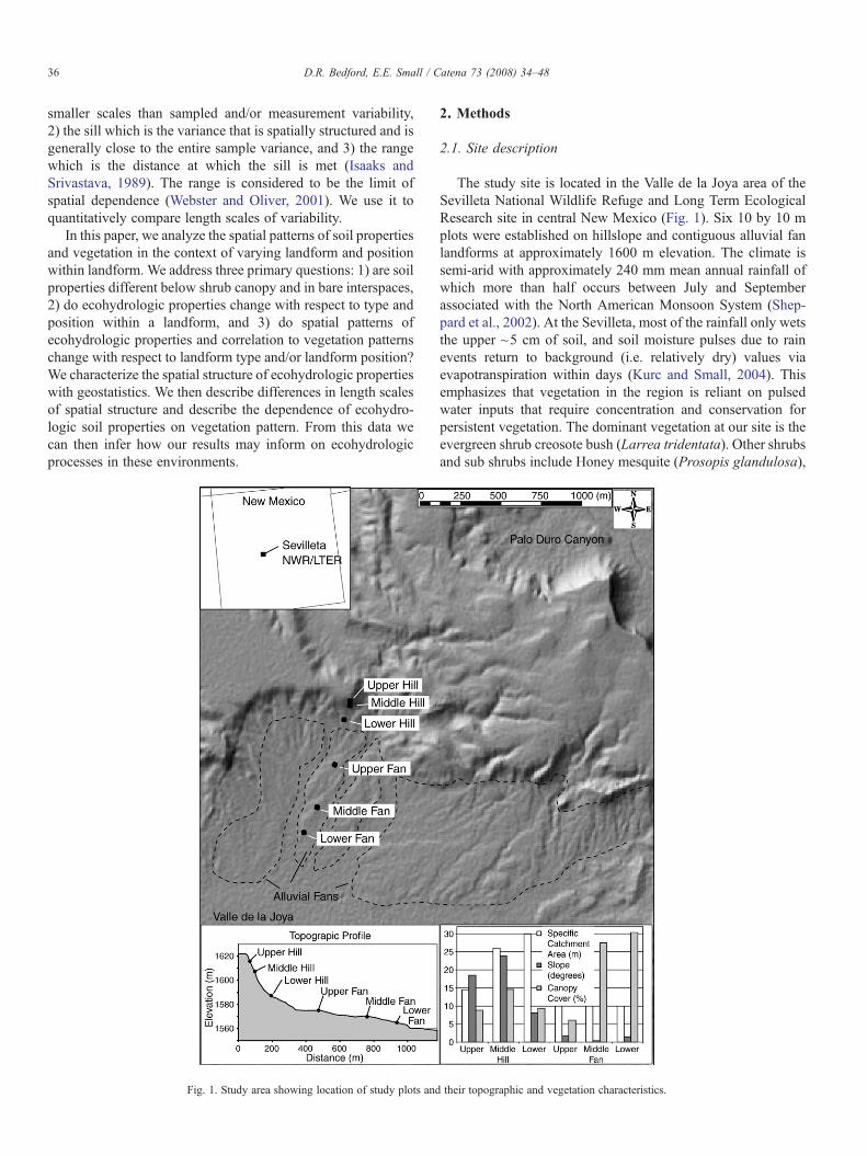
Fig. 1. Study area showing location of study plots and

2. Methods

2.1. Site description

The study site is located in the Valle de la Joya area of theSevilleta National Wildlife Refuge and Long Term EcologicalResearch site in central New Mexico (Fig. 1). Six 10 by 10 mplots were established on hillslope and contiguous alluvial fanlandforms at approximately 1600 m elevation. The climate issemi-arid with approximately 240 mm mean annual rainfall ofwhich more than half occurs between July and Septemberassociated with the North American Monsoon System (Shep-pard et al., 2002). At the Sevilleta, most of the rainfall only wetsthe upper ~5 cm of soil, and soil moisture pulses due to rainevents return to background (i.e. relatively dry) values viaevapotranspiration within days (Kurc and Small, 2004). Thisemphasizes that vegetation in the region is reliant on pulsedwater inputs that require concentration and conservation forpersistent vegetation. The dominant vegetation at our site is theevergreen shrub creosote bush (Larrea tridentata). Other shrubsand sub shrubs include Honey mesquite (Prosopis glandulosa),

their topographic and vegetation characteristics.

Fig. 3. A) Diagram of one-dimensional measurement and components oftopography (gray). Zp represents the plane parallel to the ground surface (line inone-dimension). The distance from Zp (the wire frame) to the ground surface ismeasured, including an error from sagging of the wire. Adjustment for wire sagmay include some curvature from the landform (Zl) but Zl is not explicitlyaccounted for. B) Microtopography (Zm) is defined as the perpendiculardistance of the ground surface from Zp such that the mean microZ value is 0.Shown is the profile below the wire frame in A.

37D.R. Bedford, E.E. Small / Catena 73 (2008) 34–48

Mormon tea (Ephedra torreyana), and snakeweed (Gutierreziasarothrae). Very minor bunches of perennial black grama(Bouteloua eriopoda) grass were also noted. No soil lichens orother soil crust organisms were observed.

Topographic characteristics of the plot transect are presentedin Fig. 1. The primary topographic differences betweenhillslope and alluvial fan plots are slope and drainage arearelationships. The hillslope plots have steep slopes, and the soilsare relatively thin (b1 m) and generated by local weathering.The hillslope shows characteristic trends in topographiccharacteristics such as increasing specific catchment area(drainage area per unit contour), and slight concave-up toplanar cross-section profile. The alluvial fan is contiguous withthe base of the hillslope, and likely was derived throughhillslope erosion. Some sediment was likely from the catchmentto the east of the hillslope. The alluvial fan sits 1–2 m aboverecently active stream channels. Only one soil-geomorphicsurface is present on the fan, excluding incised channels.Topographic characteristics of the alluvial fan are typical ofdivergent landforms: little to no changes in specific catchmentarea, and little to no changes in slope with landform position,and concave-down in cross-section profile.

2.2. Data collection

Measurements of microtopography, infiltration, and soiltexture were made at each 10 by 10 m plot according to thesampling scheme in Fig. 2. All infiltration and soil texturemeasurements were co-located with microtopography measure-ments. Perennial vegetation was measured as it occurs within oroverhanging the plots.

We define microtopography, Zm, as the deviation of theground surface from a plane parallel to the overall slope of the

Fig. 2. Sampling scheme for Zm (black dots, n∼1500) and Ksat (circles, n=66).

surface, over the extent of each plot. Zm is a portion of overalltopography, which can be defined as:

Z ¼ Zlþ Zmþ error ð1Þ

where Z is the ground surface elevation, Zl is the portion of Zdefined by landform topography (curvature), Zm is microtopo-graphy generally in the mm-decimeter scale, and error is ameasurement error term. At finer scales (e.g.b1 cm), differencesbetween soil particle sizes and other perturbations are sources ofelevation differences and are not addressed here. Fig. 3illustrates these components and the measurement of Zm inone-dimension.

Zm was measured using a wire frame installed parallel to theground surface as determined by eye. We determine theelevation of the frame, Zp, to be the slope of a plane over thesurface (Fig. 3). We assume that the wire frame represents Zl,and that the deviation of Zp from Zl is not a significantcomponent of topography at our plot size and locations (i.e.Zp~Zl). The distance from the wire frame to the ground wasmeasured to the nearest millimeter and the ground conditionnoted. Common ground conditions noted were bare ground,plant canopy and type, and large rocks.

The wire frame consisted of cables stretched across the plotin the upslope direction. Although the wire appeared visuallystraight, the wire had ~5 cm sag at the center. To account forsagging of the wire, which introduces the deviation from Zp andaffects Zm (Fig. 3B we solve for a parabolic error term. We fit a2nd order polynomial in the upslope direction of ourmeasurements. We then adjusted the measured wire heightsby the deviation of the parabolic fit from a datum parallel to theend-points of the wire frame (Zp). The adjusted distances fromthe wire frame to the ground are then converted to Zm bysubtracting all measured distances from the mean value of all

38 D.R. Bedford, E.E. Small / Catena 73 (2008) 34–48

measured distances for each plot. This correction also removessome secondary trend in the data due to down-slope landformcurvature, which cannot be separated from the wire sag, and areassumed to be negligible. In short, Zm values are all relative to adatum, the mean plane ‘fitted’ to the area of the plot: negativeZm values are below the plane, and positive are above.

Infiltration rate is a complex function of soil water contentsand potentials through time, thus we simplify using a singlevalue to describe infiltration. We use saturated conductivity(Ksat), which is the minimum infiltration rate that would beobserved under unlimited water application conditions. Wedetermined Ksat with single-ring constant head infiltrometers.The infiltrometer rings are 5 cm in diameter, and were insertedto a depth of 5 cm. A 5 cm head (ponding depth) wasmaintained in the rings with the use of Marriotte tubes. A datalogger and pressure transducer measured pressure in theMarriotte tubes every 5 s. Pressure in the Marriotte tubechanges as a calibrated linear function of the rate of water dropin the tubes, which is the rate of “field” infiltration. Infiltrationwas allowed to progress for 35–45 min to allow the infiltrationto approximate steady state. Our “field” infiltration ratesactually represent 3-d flow in the soil, the characteristics ofwhich are predominantly affected by ring geometry, pondingdepth, and soil properties (Reynolds and Elrick, 1990). Weapproximate true, 1-dimensional, Ksat rate by using the methodof Wu et al. (1999) which states that field determined infiltrationis ~ f-times larger than true 1-dimensional infiltration rate. Themethod of Wu et al. (1999) accounts for the ring and soilproperties, as well as the time-series of each individualinfiltration measurement. For our data, f is approximately 2.3,but varies with soil texture. We determined soil texture at thelocation of each Ksat measurement with the methods of Kettleret al. (2001). We then quantified the necessary values forcalculating the f parameter with the Rosetta software program(Schaap et al., 2001).

Perennial vegetation was measured manually and surveyedwith a Total Station. The maximum height, maximum canopywidth, canopy width perpendicular to the maximum width, andtwo basal widths were measured with a meter stick, to the nearestcentimeter. We also surveyed the locations of the basal center,and the maximum and perpendicular to maximum canopy widthsusing a Total Station. The Total Station survey of the basal centerand maximum widths (as above) is used to calculate coverbecause it accounts for plant canopies that overlap. Basal widthrefers to the width of all shrub stems or grass clump entering theground surface, the center of which is estimated by eye. We thencalculated per-plant average width and basal width, as well ascanopy area and volume. We calculated canopy area assuming acircular area rather than an elliptical area using the average of ourwidth measurements. Our volume calculations for all plantspecies follow Hamerlynck et al. (2002), assuming a truncated,inverted cone shape with:

Volume ¼ 1=3½ �pH W=4ð Þ2þ B=4ð Þ2þ W=4þ B=4ð Þh i

ð2Þ

whereH is the maximum height,W is the average width, and B isthe average basal width.

We determined the spatial pattern of vegetation by quantifyingPlant Distance (PD), which is the distance to the nearest shrub basefor every location in the plot. We calculated PD because we wish todetermine how ecohydrologic properties vary as a function of dis-tance from plants, as well as how plant patterns may change acrosslandforms. PDvalues therefore enable characterization of vegetationpattern via univariate statistics and geostatistics. Significant relation-ships to other properties such as Zm and Ksat can then be used inextrapolation such as cokriging. This method is an inversion oftraditional point pattern analysis where distances from isolatedpoints, such as plant centers to their nearest neighbor(s), are calcu-lated (e.g. Dale, 1999). We discretized each plot area into 5 by 5 cmgrids, and for every grid location we calculated the Euclideandistance to the nearest shrub base as determined by the Total Stationsurvey. We did not differentiate plant species or functional types inthis analysis. We used the base of the shrub as the datum for PD asopposed to canopy edge because initial data explorations showedthat the data were more strongly related to PD calculated from theshrub base.

2.3. Statistics

Most of our statistical techniques assume normally distributedpopulations.We used probability (Q–Q) plots to qualitatively checkfor normality, andwe test for normality with the Shapiro–Wilk'sW-statistic (Insightful Corporation, 2001). The W-statistic is limited topopulations of less than 5,000 ata points and cannot be computed forPD (N40,000 samples per plot). For PD, we use Q–Q normalprobability plots to qualitatively determine normality. Probabilityplots suggested that Zm is relatively normally distributed, the ex-ception being at the far end of both tails of the distributions. W-statistics for Zm are high, but p-values were not sufficient todefinitively describe the data as normal. Because the data divergefromnormal only at the extreme tails, have low skewness, and donotapproximate other distributions with reliable back-transforms, wedetermine that Zm roughly approximates a normal distribution.Probability plots and W-statistics for Ksat show that the data arenormally distributed following a log-10 transform. Probability plotsand summary statistics suggest that PD approximates a normaldistribution when the data is square root transformed.

We use pairedF-tests and Anova methods to test for differencesbetween population variances and means, respectively. We test fordifferences between landforms, plots (i.e. testing for the effect oflandscape position), and between canopy and interspace withinplots. Because Zm at each plot has a mean of zero, we cannot usethe Anovamethods to test for differences in sample means, thus weuse F-tests with permutations of plot combinations to test fordifferent Zm variances between plots. All other data, including Zmbetween canopy and interspace, are tested with Anova and Tukey’smultiple comparisonmethods. In all cases, we perform a two-tailedtest at 95% confidence with the null hypothesis being that thepopulation means (or variances for Zm across plots) are equal.

2.4. Geostatistics

We use geostatistics to quantify spatial patterns. Omnidirectionalexperimental variograms and cross-variograms are calculated, and

Table 1Summary statistics and statistical differences for vegetation measurements

Comparison Height (cm) Anova1 Average width (cm) Anova1 Average base (cm) Anova1 Canopy area (m2) Anova1 Volume (m3) Anova1 Cover (%)

Hillslope 71±26 A 96±38 A 13±6 A 0.8±0.5 A 0.23±0.19 A 11Alluvial Fan 102±28 B 133±45 B 21±7 B 1.5±1.1 B 0.62±0.57 B 22Upper Hill 59±29 A 83±39 A 11±5 A 0.7±0.5 A 0.17±0.15 A 9Middle Hill 80±26 A 104±30 A 14±6 A 0.9±0.5 AC 0.28±0.20 B 15Lower Hill 67±16 A 97±36 A 15±6 AC 0.8±0.6 AC 0.21±0.19 AB 9Upper Fan 76±18 A 104±25 A 22±5 B 0.9±0.4 AD 0.26±0.14 ABC 6Middle Fan 107±21 B 149±49 B 23±8 B 1.9±1.3 BD 0.79±0.66 C 28Lower Fan 112±29 B 134±43 B 18±7 BC 1.6±1.0 BCD 0.67±0.56 C 301 Different letters denote different means at 95% confidence level.

Table 2Summary statistics and statistical differences for Zm and PD between landforms,plots and mosaic components

n Mean UpperQuartile(moundheight)

Differentvariance(F-test)1

Differentmean(Anova)1,2

Percentdifference(interspacevs canopy)

Zm (cm)Interspace 6964 −0.3±3.1 – A ACanopy 2068 0.9±4.0 3.3 B B 133Hillslope 4553 0±4.1 A – –Interspace 3502 −0.2±3.9 – a2 a2

Canopy 1051 0.7±4.8 3.9 b2 b2 129Alluvial Fan 4479 0±2.4 B – –Interspace 3462 −0.3±2.1 – a2 a2

Canopy 1017 1.0±2.9 2.9 b2 b2 130Upper Hill 1538 0±5.0 A – –Interspace 1266 −0.2±4.9 – a2 a2

Canopy 272 0.8±5.6 5.6 b2 b2 125Middle Hill 1477 0±4.8 B – –Interspace 1002 −0.2±4.4 – a2 a2

Canopy 475 0.5±5.4 4.2 b2 b2 140Lower Hill 1538 0±1.8 C – –Interspace 1234 −0.2±1.5 – a2 a2

Canopy 304 0.9±2.3 2.5 b2 b2 122Upper Fan 1538 0±1.9 D – –Interspace 1353 −0.2±1.7 – a2 a2

Canopy 185 1.5±2.1 2.9 b2 b2 113Middle Fan 1453 0±2.8 E – –Interspace 1090 −0.4±2.6 – a2 a2

Canopy 363 1.1±3.1 3.2 b2 b2 136Lower Fan 1488 0±2.5 F – –Interspace 1019 −0.4±1.9 – a2

Canopy 469 0.8±3.2 2.5 b2 150

PD (cm)Upper Hill 40,401 92±50 – – A –Middle Hill 40,401 96±51 – – BLower Hill 40,401 127±76 – – CUpper Fan 40,401 138±72 – – DMiddle Fan 40,401 113±57 – – ELower Fan 40,401 106±60 – – F

Comparisons with different letters are significantly different: Large lettersdenote differences between plots, and small letters denote differences betweenmosaic components.1 Different letters denote differences at 95% confidence level.2 Within-plot differences.

39D.R. Bedford, E.E. Small / Catena 73 (2008) 34–48

we fit theoretical variograms numerically. We then use (cross-)variogram parameters, specifically the range, to quantify the extentof spatial variability. We use transformed values that approximate anormal distribution for all calculations.

We calculate the univariate semivariogram with:

g hð Þ ¼ 12N hð Þ

� �XN hð Þ

i¼1

xiþh � xið Þ2 ð3Þ

where h is a separation vector between measurements, N(h) isthe number of measurement pairs, x is the data values atlocations xi and xi+ h (Deutsch and Journel, 1998).

We calculate the bivariate cross-semivariogram with:

gZY hð Þ ¼ 12N hð Þ

� �XN hð Þ

i¼1

zi � ziþhð Þ yi � yiþhð Þ ð4Þ

where zi is the value of attribute z, zi + h is the value at thelocation separated by vector h, and yi is as z except for the otherattribute (Deutsch and Journel, 1998). We rescale data values torange from 0 to 1 in order to equally compare values withdifferent units (Deutsch and Journel, 1998) with:

xV¼ x� xminð Þxmax � xminð Þ ð5Þ

where x′ is the rescaled value, x is the original value and xmin andxmax are theminimum andmaximum values of x, respectively.Welimit variograms to a maximum separation of 7 m, which is one-half the maximum distance between measured points, and isconsidered the largest reliable sampling domain (Deutsch andJournel, 1998). In some cases, we limit the maximum distance toless than 7 m in order to achieve closure on fitting routines.

We fit variogram models mathematically as opposed tofitting by eye. In order to place confidence intervals onvariogram model parameters with which to compare para-meters, we adopted a rigorous statistical method for as-sessing the variogram and its parameters. There are threelevels of statistical rigor for mathematically fitting vario-grams: ordinary least squares fits, weighted least squares(WLS), and generalized least squares (GLS). WLS is themost commonly used variogram fitting method where lagvariogram values are given weights according to the numberof sample pairs, or the variance associated with the variogram

lag (e.g. Cressie, 1985; Jian et al., 1996). GLS incorporates boththe sampling variance and/or the correlation of lag variogramvalues that arises from samples being used in multiple lag

Fig. 4. Box plots of ecohydrologic properties divided by plot and mosaic component. A) Microtopography (Zm), saturated conductivity (Ksat), and distance from plantcenter (PD). Letters denote significant differences of means at 95% confidence; large letters denote differences between plots, and lowercase letters denote differencesbetween mosaic components. Boxes denote sample 25% and 75% quartiles, line within box is the mean, whiskers are 5% and 95% percentiles, and horizontal linesoutside whiskers are outliers. For A, the dashed line in the background is the mean (0) value.

40 D.R. Bedford, E.E. Small / Catena 73 (2008) 34–48

averages (Pardo-Iguzquiza andDowd, 2001; Pelletier et al., 2004;Zimmerman and Zimmerman, 1991). Pardo-Iguzquiza and Dowd(2001) claim that WLS is too crude to use for calculatingconfidence intervals of variogram parameter, however therecurrently is no method for assessing cross-variogram uncertaintywithGLS in the literaturewe found.Other authors have found thatwhile GLS methods perform best, WLS is often sufficient,particularly for simple variogram parameters such as the rangeand sill particularlywhenWLSweights were determined from thenumber of pairs or sampling variance in each lag (Pelletier et al.,2004; Zimmerman and Zimmerman, 1991).

We fit theoretical variogram and cross-variogram models withWLS techniques and assign lag weights using the lag sampling

variance. We calculate the variance of a semivariogram lag ac-cording to Cressie (1985):

Var g hð Þ½ � ¼ 2 2g hð Þ½ �2N hð Þ ð6Þ

where γ(h) and N(h) are calculated from Eq. (3). For variance ofcross-variogram lags,we take the approachof Pelletier et al. (2004)and calculate the variance according to:

Var gZY hð Þ½ � ¼ g 2ZY þ gZ hð Þ⁎gY hð Þ½ �

N hð Þ ð7Þ

Table 3Summary statistics and statistical differences for Ksat between landforms, plotsand mosaic components

Ksat (cm hour−1) n Mean Different Different Percent

41D.R. Bedford, E.E. Small / Catena 73 (2008) 34–48

where γZY (h), is calculated from Eq. (4), and γz and γy arecalculated for each variable z and y with Eq. (3).

Inspection of our experimental variograms suggested thatspherical, nested spherical with hole effect, and Gaussianmodels are likely most appropriate for experimental models.Hole effects are typical when properties have repetitive or cyclicstructure such as vegetation patches. For consistency, we use asimple spherical model for fitting all of our data. Sphericalvariograms are modeled with:

g hð Þ ¼ C0 þ C⁎1 1:5

hrange

� 0:5h

range

� �3" #

; hb range

C0 þ C1; hzrange

8><>:

9>=>;ð8Þ

where C0 is the nugget effect, C1 is the spatially structuredvariance, and h is as above (Deutsch and Journel, 1998). Thesill is the sum of C1 and C0.

We fit our models using the package NLME version 3(Pinheiro and Bates, 2000) in S-plus version 6 (InsightfulCorporation, 2001). We also calculated simultaneous standarderrors on model parameters to assess parameter uncertainty withNLME.

We determined the spatial scale of ecohydrologic propertieswith the semivariogram range, and use its standard error todiscuss its uncertainty and differences. We determine thecorrelation length scales between vegetation pattern and soilproperties as the range of the soil property-PD cross-variogram.

variance(F-test)1

mean(Anova)1

difference(interspace vscanopy)

Interspace 263 4.86±2.82 A ACanopy 97 6.54±3.66 A B 35Hillslope 172 4.02±2.34 A AInterspace 127 3.84±1.98 a2 a2

Canopy 45 4.56±3 a2 a2 19Alluvial Fan 188 6.48±3.36 A BInterspace 136 5.76±3.12 a2 a2

Canopy 52 8.28±3.3 a2 b2 44Upper Hill 58 4.62±2.4 – AInterspace 45 4.26±1.74 a2 a2

Canopy 13 5.88±3.84 a2 a2 38Middle Hill 65 4.44±2.4 – AInterspace 42 4.2±2.16 a2 a2

Canopy 23 4.86±2.82 a2 a2 16Lower Hill 60 3.12±1.86 – AInterspace 48 3.24±1.98 a2 a2

Canopy 12 2.52±1.14 a2 a2 −22Upper Fan 60 5.58±2.64 – BInterspace 45 4.8±2.04 a2 a2

Canopy 15 7.98±2.82 a2 b2 66Middle Fan 64 6.3±2.58 – BInterspace 43 5.34±2.22 a2 a2

Canopy 21 8.22±2.16 b2 b2 54Lower Fan 62 7.56±4.26 – BInterspace 46 7.2±4.08 a2 a2

Canopy 16 8.58±4.74 a2 a2 19

Comparisons with different letters are significantly different: Large lettersdenote differences between plots, and small letters denote differences betweenmosaic components.1 Different letters denote differences at 95% confidence level.2 Within-plot differences.

3. Results

3.1. Vegetation measurements

We found that shrubs are significantly smaller on the hillslopethan on the alluvial fan (Table 1). There are no clear patterns ofdifferences between individual plots on a landform, suggestingthat landform type is a key determinant of vegetation character-istic at our site. However, the general trend of plant measures wasfor them to increase down the hillslope–alluvial fan transect.Qualitatively, we also found that there is more variety of specieson the hillslope, including a wider diversity of sub shrubs.

PD, our measure of distance to the nearest plant center issignificantly different between all of the plots at the 99%confidence level (Table 2, Fig. 4). However, we caution thatdifferences in PD on the order of 10 cm are likely notecologically significant (i.e. differences between Upper andMiddle Hill are not strong). Mean PD generally increased downthe hillslope, with smallest values at the steepest middle plot,showing that plants are getting more spread apart, potentially inresponse to slope. Conversely, PD decreased down the alluvialfan transect, showing that plants are getting closer and/or larger.

3.2. Zm relations to vegetation and landform

We found that microtopography, Zm, is on average 133%higher under vegetation canopy than in interspace, showing the

presence of shrub mounds (Table 2 and Fig. 4). Despite plotsurfaces being overall fairly rough, shrub mounds are present onall plots regardless of landforms and positions within landform.

The average difference between mean interspace and canopyZm across all plots is 1.2 cm. The mean difference varies acrossplots, from 0.7 to 1.7 cm. Mean Zm under canopy is not a goodindicator of shrub mound height. On a per-plant basis, the shrubmound height would be themaximumZm value, but our data doesnot allow this determination. Therefore we consider the upper, 3rd,quartile of our Zm measurements under canopy as an indicator ofthe magnitude of plot-average shrub mound height. Overall, theaverage height of shrub mounds is 3.3 cm, but on hillslopes theaverage is 3.9 cm and 2.9 cm on alluvial fans (Table 2, Fig. 4). Wedetermined roughness via the variance of Zm. Zm under shrubcanopy is always more rough than interspaces within a plot. Inaddition to microtopography being higher under shrub canopy, wealso found that plot-wide microtopography was significantlyrougher on the hillslope than the alluvial fan (Table 2).

These results suggest that vegetation, landform type, andposition within landform are strong determinants of micro-topography. We observed mounds under shrubs on all plots;hillslopes are rougher and have tall and rough shrub mounds.

Fig. 5. Relationships of Zm and Ksat to distance from plant center (PD) for the Lower Fan plot. Shaded area represents average shrub radius, horizontal lines portraythe mean value.

42 D.R. Bedford, E.E. Small / Catena 73 (2008) 34–48

Alluvial fans are overall smoother and much of the micro-topography is under shrubs.

3.3. Ksat relations to vegetation and landform

We found that Ksat is significantly higher (by 35%) undershrub canopy (Table 3, Fig. 4) when all of the data is subdividedonly by interspace-canopy. This relationship only statisticallyholds true on alluvial fan plots, where Ksat is 19–66% higherunder canopy. However, on hillslope plots, Ksat is slightlyhigher under canopy but statistically equal. At the Lower Hillplot, Ksat was actually ∼22% lower under canopy.

Pooled by landform, plot-averaged Ksat is ∼60% greater(significant at 95%) on alluvial fan plots than on hillslope plots(Table 3). The mean Ksat rate is not statistically differentbetween all plots, suggesting that the landform is a strongdeterminant of plot-averaged Ksat (Table 3, Fig. 4). Despite thelack of significant differences of mean Ksat values within alandform, there are subtle trends with respect to position withinlandform. In general, mean Ksat rates decreases down thehillslope and slightly increases down the alluvial fan, from headto toe. In short, hillslopes have lower mean Ksat rates, andalluvial fans have higher mean Ksat rates. We detected nosignificant difference in mean Ksat rate as a function of positionwithin landform.

Our Ksat measurements have a range of ∼15× (from 1.08 to16.80 cm/h), which is a relatively small range compared topublished Ksat values, such as in Rawls et al. (1983), whichrange from 0.03 to 11.78 cm/h, a factor of over 500×. Theseresults show that for related landforms, there is an overall smallrange of Ksat. Yet within that range, there is random variability inaddition to variability described by the presence of shrub canopy.

In summary, plots on hillslopes have small plants with lowcover, rough microtopography and low Ksat rates. Shrub

mounds are tall and there is no significant difference in Ksatunder shrubs versus interspace. Plots on the alluvial fans havetaller, wider shrubs, with more cover, smooth, low-amplitudeinterspace microtopography, and higher Ksat rates. Shrubs onalluvial fans have taller mounds, and also have higher Ksat ratesrelative to interspaces beneath them.

3.4. Spatial patterns

We found that soil properties are strongly related to thepattern of vegetation, and that the effect of vegetation on soilproperties extends beyond vegetation canopy. For example,Fig. 5 shows that both Zm and Ksat are high under shrub canopy(shaded area) and tend to decrease with distance away fromshrubs (increasing PD). This decrease with distance and themagnitude of differences vary by landform and vegetationcharacteristics, which we show with geostatistics.

We fit variogram models to quantify the distance over whichecohydrologic soil properties are spatially structured, equal to therange. Examples of our variograms are displayed in Fig. 6.Despite a simple variogram model, most data were fitted well.Ksat variograms, however, were generally not fitted very well.This is largely due to two factors: sparse sampling, and likely largeamounts of random variability. All Zm variograms show clearvariogram features such as a sill and range, with the exception ofthe Upper Hill plot. Zm variograms from this plot do not show astrong sill feature, indicative of a trend in the data. We interpretthat this trend arose from cross-slope curvature of the plot surfacethat was not accounted for in our measurements, yet is visuallyapparent in the field. Because of this trend, we expect rangeestimates for this plot to be inaccurate and represent the trend asopposed to the scale of the local variability. We feel a betterestimate of the range for the Upper Hill plot is slightly less than2m, but present all results with the fitted values.We estimated the

Fig. 6. A) Example variograms of Zm from all plots. Dots denote variogram lags used to fit the variogram model, shown as a line; crosses denote data not used in thefitting. B) Zm, Ksat, PD variograms and Zm-PD, Ksat-PD cross-variograms from Lower Fan plot.

43D.R. Bedford, E.E. Small / Catena 73 (2008) 34–48

Upper Hill Zm range atb2 m from a slight flattening of thevariogram thatmay indicate a sill in the absence of a trend (Fig. 6).

We found that all of the properties show spatial patternscommonly ∼1.5–3 m in scale (Table 4 and Fig. 7), whereas theaverage shrub radius isb1 m (Table 1). These patterns werestrongly related to the vegetation pattern, and extended 3–4times beyond the edge of vegetation canopy. The average rangeof all variograms is 2.5 m. As Fig. 7 shows, range parameters

for most of our variograms change with respect to landformtype, and for some data with position on the landform.Assuming that the range for Zm on the Upper Hill is less than2 m, the ranges for Zm, Ksat, and PD tend to be smaller onhillslopes than on fans.

The average range of cross-variograms, representing thescale of co-variability, is 1.6 m (Fig. 7). Small standard errors oncross-variograms for Zm-PD suggest that there is a strong

Table 4Fitted variogram and cross-variogram model parameters for ecohydrologicproperties

Plot Zm Ksat PD Zm-PD Ksat-PD

Upper Hill 3.3±0.1 0.9±0.7 2.3±0.1 1.2±0.9 1.5±3.1Middle Hill 2.1±0.1 0.4±0.7 2.4±0.1 1.5±0.4 0.7±3.1Lower Hill 1.8±0.1 1.6±1.6 3.9±0.1 2.0±0.2 2.1±2.4Upper Fan 1.9±0.1 5.0±2.2 3.7±0.1 3.0±0.2 1.2±1.2Middle Fan 2.2±0.1 4.5±2.3 2.7±0.1 1.3±0.2 1.4±0.7Lower Fan 2.8±0.1 1.1±1.2 3.1±0.1 1.3±0.1 2.0±3.1Mean Hill 2.4 1.0 2.9 1.6 1.4Mean Fan 2.3 3.5 3.2 1.9 1.5Mean 2.4 2.3 3.0 1.7 1.5

Note: bold values are not significant at 95% confidence.

Table 5Percentages of plot area showing spatial structure associated with vegetationpattern

Plot Zm (%) Ksat (%)

Upper Hill 73 61Middle Hill 84 32Lower Hill 86 87Upper Fan 99 49Middle Fan 66 67Lower Fan 72 93

Proportions defined as the aerial percent of PD measurements within the rangeof the cross-variogram for each property.

44 D.R. Bedford, E.E. Small / Catena 73 (2008) 34–48

spatial correlation between these two variables. This is alsosupported by the ranges for Zm-PD to mimic those of PD,roughly by a factor of one-half those of PD. Cross-variogramsfor Ksat-PD have large standard errors again, due to acombination of small Ksat sample numbers, simple variogrammodel, and apparent random variability in Ksat. However, theaverage Ksat-PD range is 1.5 m, suggesting that this may be acommon correlation distance for these soils.

We found that the scale of ecohydrologic properties wassimilar in magnitude to the scale of vegetation-associatedpatterns (i.e. the range of Zm is similar to the range of Zm-PD).From this we conclude that the pattern of soil properties isdependant on the vegetation pattern. This is further supportedby smaller standard errors on variograms and their parameters.

Fig. 7. Range and standard error of fitted variogram and cross-vario

It is also important to note that the scale of soil variabilityassociated with shrub canopies is much larger than the scale ofthe shrub canopy itself. This is illustrated in two ways. First, wecompare the proportion of space covered by vegetation canopycover, to the range of canopy-associated variability. We usedour maps of PD to calculate the proportion of plot area withinthe range of cross-variogram parameters. Table 5 and Fig. 8show that the proportion of space exhibiting spatial structure ofZm and Ksat vary with landform and position within landform,although not in an apparent systematic way. Second, wecompare the size of shrubs to the size (scale) of shrub-associatedvariability: the percent space affected by shrubs is larger thanthe space occupied by shrubs. The average space exhibitingspatial variability is ∼75%, while the average cover is 16% andthe maximum is 30% (Table 1). This is further demonstrated bypointing out that the average radius of shrub canopy is ∼56 cm,while the range of spatial variability associated with shrubs is

gram models. A) Zm, B) Ksat, C) PD, D) Zm-PD, E) Ksat-PD.

Fig. 8. Proportions of PD plot area within the range of cross-variogram parameter, representing the percent space affected by shrub-related ecohydrologic properties.Crosshatches denote canopy cover in percent.

45D.R. Bedford, E.E. Small / Catena 73 (2008) 34–48

commonly 1.5–2 m, roughly 3–4 times the size of shrubcanopy.

4. Discussion

We found that there are differences between hillslope andalluvial fan landforms with respect to vegetation and associatedpatterns of soil ecohydrologic properties, summarized in Fig. 9.Hillslope plots have smaller shrubs. On hillslopes, shrubmounds are taller than those on alluvial fans, but relativelysmall compared to the large roughness that exists in hillslopeinterspaces. There are no statistical differences between canopyand interspace Ksat on the hillslope. Microtopography is higherand rougher, and Ksat lower, on hillslopes than on alluvial fans.Alluvial fan plots have larger shrubs with more cover. The shrubmounds are tall compared to the relatively low-relief inter-spaces. High Ksat rates under shrubs decrease away from plantcenters and extend much farther than the canopy. Our data alsosuggest that vegetation more strongly affects ecohydrologicproperties on alluvial fan plots than on hillslope plots. This isshown for Zm in that higher microtopography is more oftenfound under shrubs on alluvial fans, as well as the majority ofalluvial fan roughness occurring under shrub canopy. We also

Fig. 9. Sketch showing the relative magnitudes of microtopography and Ksat in relatithere is vegetation-related microtopography in the form of shrub mounds as well as sigincrease in Ksat under or near shrubs. On alluvial fans, both microtopography and Ksnearly the entire interspace area is affected by the pattern of vegetation.

only found significantly higher Ksat under shrub canopy onalluvial fan plots.

Our findings are similar to those in many other semi-aridlandscapes. We observed microtopography under shrubs (shrubmounds) on the order of 3–4 cm, which are similar in height toshrubmounds in southernNewMexico (Gile et al., 1998), Arizona(Parsons et al., 1992), Australia (Dunkerley, 2000), and south-eastern Spain (Bochet et al., 2000). The similarity or microtopo-graphy across regions is likely a result of the same processesinteracting with morphologically similar vegetation. In most ofthese examples mound formation was determined to be fromdifferential rainsplash and/or overland flow erosion. Furthermore,in SE Spain there was nearly twice as much runoff from erosionalhillslopes than constructional alluvial fans (Nicolau et al., 1996).This suggests that given the same governing processes, the effectsare moderated by vegetation and landform characteristics.However, these results show that mounds under morphologicallysimilar plants can be expected to be similar given similar soil andclimate contexts. This is because they develop due to a dynamicinteraction between landforms, rainfall, vegetation, diffusiverainsplash, and overland flow erosion.

Infiltration rates have been widely observed to vary betweensub-vegetation and non-vegetated interspaces. Most studies have

on to vegetation on common arid land landforms at our study site. On hillslopesnificant microtopography in the interspaces. On hillslopes there is no significantat are high under shrubs and decrease with distance away from shrubs such that

Table 6Mean canopy to interspace infiltration ratios for a variety of patchy vegetationecosystems

Source Vegetation type Canopy:interspace ratio

This report Larrea 1.3Bhark and Small Larrea only 1.2Bhark and Small Larrea and grass 1.6Cerda 1997 Stipa tenacissima 2.2Eckert and others Larrea 2.6Lyford and Qashu Larrea and paloverde 3.1Dunkerley 2002 Mulga groves 5.1Dunkerley 2000 Maireana shrubs 5.3

46 D.R. Bedford, E.E. Small / Catena 73 (2008) 34–48

focused only on the magnitude of infiltration differences betweenvegetation sub-canopy and interspace, and our results are similar toother small-scale infiltration measurements in a wide variety ofecosystems (Table 6). These data show that infiltration undervegetation is ∼30–500% greater than in interspaces. Ourmeasurements are very similar to the measurements of Bharkand Small (2003) made ∼5 km away, as well as tussock grass inSpain (Cerda, 1997).Larrea shrublands in theMojave Desert have250–300% higher infiltration rates under shrubs than interspaces(Eckert et al., 1979; Lyford and Qashu, 1969), and isolated shrubsand vegetation groves in Australia have∼500% higher infiltrationunder vegetation (Dunkerley, 2000; Dunkerley, 2002). Weinterpret the relatively low differences in values found at theSevilleta to be a result of the relatively recent encroachment ofshrubs into the region. However, it is still unknown what the timescales are of infiltration modification associated with shrubs, andparticularly if the development of high infiltration under and nearshrubs will continue to progress on somewhat stabilized (i.e.alluvial fan) landforms. On our steep hillslope, the effects ofvegetation on infiltration are likely moderated by the down-slopemovement of sediments.

While most authors have focused only on the differences inKsat between vegetation canopy and interspaces, Dunkerley(2000), and Lyford and Qashu (1969) showed that infiltrationrates, while high under shrubs, decay as a function of distance fromshrub stem center. Their results agree with our findings that Ksat isclosely related to distance fromplant centers, especially for alluvialfan landforms. Dunkerley (2000) found that zones of high Ksatextended 3.3 times farther than plant canopy edges. We found thatfor bothKsat andZm, the extent of influence of shrub canopy is 2–4 times the canopy radius. These results are important to notebecause they suggest that for many semi-arid landscapes, deter-mining soil properties based on vegetation cover alone will under-estimate the actual areal extent of vegetation-like soil properties.

Our results show that given similar soil characteristics,landform type and vegetation pattern are strong determinates ofsmall-scale variability in soil properties. This is likely a responseto differing magnitudes of surface processes that occur on theselandforms. Hillslopes have steep slopes and likely have sedimentfluxes across the surface over reasonably short time scales. Thiswill likely result in the erasure of the effects that vegetation hason surface processes. Conversely, gently sloping alluvial fansurfaces likely remain constructional through time as a result ofrelatively low net sediment fluxes (i.e. local redistribution ofsediment). The relative stability of alluvial fan surfaces allows the

feedbacks associated with vegetation canopy to progress,resulting in stronger vegetation-dependant soil properties.

These results have repercussions on the geomorphologicaland ecological dynamics of these landforms. We have shownthat vegetation size and amounts, as well as the variability ofsoil properties, are dependent on the type of landform, and maybe dependant on position within the landform. This suggeststhat landforms, and potentially different landform positions,will respond differently to rainfall events. This has strongimplications for the long-term dynamics of sediment acrossthem, and therefore landform evolution, as has been theorizedand modeled (e.g. Collins et al., 2004; Istanbulluoglu and Bras,2005). Furthermore, our results show that landform-dependantprocesses may affect the local redistribution of water andsediment. Redistribution has been attributed to the creation andmaintenance of patterned mosaic vegetation on hillslopes in avariety of environments (Bergkamp, 1998; Bergkamp et al.,1996; Ludwig et al., 2005; Puigdefabregas, 2005; Sanchez andPuigdefabregas, 1994; Wilcox et al., 2003). Breshears (2006)also hypothesized that environments with moderate canopycover may be more susceptible to landscape change, and ourresults suggest that hillslope environments, because of relative-ly low to moderate cover and relatively little modification of thesoil beneath canopy, may be more susceptible to landscapechange. Despite the apparent role of redistribution in concen-trating resources, a key part of arid land ecologic functioning,the processes driving redistribution processes have generallynot been studied, and it remains to be determined under whatconditions, and to what extent, redistribution occurs.

Acknowledgements

This work was supported by the U.S. Geological Survey andSAHRA (Sustainability of semi-Arid Hydrology and RiparianAreas). We thank reviewers Laure Montandon, Ethan Gutmannand two anonymous reviewers who contributed greatly to themanuscript. John Felis, Angeles García Mayor, and Gus Legergave assistance in the field. The staff at the Sevilleta LTER andNational Wildlife Refuge provided access and logistical support.

References

Alizai, H.A., Hulbert, L.C., 1970. Effects of soil texture on evaporative loss andavailable water in semi-arid climates. Soil Science, 110 (5), 328–&.

Bergkamp, G., 1998. A hierarchical view of the interactions of runoff andinfiltration with vegetation and microtopography in semiarid shrublands.Catena 33 (3–4), 201–220.

Bergkamp, G., Cammeraat, L.H., Martinez, F.J., 1996. Water movement andvegetation patterns on shrubland and an abandoned field in two desertification-threatened areas in Spain. Earth Surface Processes and Landforms 21 (12),1073–1090.

Bhark, E.W., Small, E.E., 2003. Association between plant canopies and thespatial patterns of infiltration in shrubland and grassland of the ChihuahuanDesert, New Mexico. Ecosystems 6, 185–196.

Bochet, E., Poesen, J., Rubio, J.L., 2000. Mound development as an interactionof individual plants with soil, water erosion and sedimentation processes onslopes. Earth Surface Processes and Landforms 25 (8), 847–867.

Bowers, M.A., Lowe, C.H., 1986. Plant-form gradients on Sonoran Desertbajadas. Oikos 46 (3), 284–291.

47D.R. Bedford, E.E. Small / Catena 73 (2008) 34–48

Breshears, D.D., 2006. The grassland-forest continuum: trends in ecosystemproperties for woody plant mosaics. Frontiers in Ecology and the Environment4 (2), 96–104.

Breshears, D.D., Nyhan, J.W., Heil, C.E., Wilcox, B.P., 1998. Effects of woodyplants on microclimate in a semiarid woodland: soil temperature andevaporation in canopy and intercanopy patches. International Journal ofPlant Sciences 159 (6), 1010–1017.

Brown, K.J., Dunkerley, D.L., 1996. The influence of hillslope gradient, regolithtexture, stone size and stone position on the presence of a vesicular layer andrelated aspects of hillslope hydrologic processes: a case study from theAustralian arid zone. Catena 26 (1–2), 71–84.

Bull, W.B., 1977. The alluvial-fan environment. Progress in Physical Geography1 (2), 222–270.

Burke, I.C., et al., 1999. Spatial variability of soil properties in the shortgrasssteppe: the relative importance of topography, grazing, microsite, and plantspecies in controlling spatial patterns. Ecosystems 2 (5), 422–438.

Canfield, H.E., Lopes, V.L., Goodrich, D.C., 2001. Hillslope characteristics andparticle size composition of surficial armoring on a semiarid watershed in thesouthwestern United States. Catena 44 (1), 1–11.

Cerda, A., 1997. The effect of patchy distribution of Stipa tenacissima L onrunoff and erosion. Journal of Arid Environments 36 (1), 37–51.

Cerda, A., 1998. The influence of geomorphological position and vegetationcover on the erosional and hydrological processes on a Mediterraneanhillslope. Hydrological Processes 12 (4), 661–671.

Clothier, B.E., Scotter, D.R., Kerr, J.P., 1977.Water-retention in soil underlain by acoarse-textured layer—theory and a field application. Soil Science 123 (6),392–399.

Collins, D.B.G., Bras, R.L., Tucker, G.E., 2004. Modeling the effects ofvegetation-erosion coupling on landscape evolution. Journal of GeophysicalResearch-Earth Surface 109.

Cressie, N., 1985. Fitting variogram models by weighted least-squares. Journalof the International Association for Mathematical Geology 17 (5), 563–586.

Cross, A.F., Schlesinger, W.H., 1999. Plant regulation of soil nutrient distributionin the northern Chihuahuan Desert. Plant Ecology 145 (1), 11–25.

Dale, M.R.T., 1999. Spatial Pattern Analysis in Plant Ecology. CambridgeUniversity Press, Cambridge. 326 pp.

Deutsch, C.V., Journel, A.G., 1998. GSLIB Geostatistical Software Library andUser's Guide. Oxford University Press. 369 pp.

Dunkerley, D., 2000. Hydrologic effects of dryland shrubs: defining the spatialextent of modified soil water uptake rates at an Australian desert site. Journalof Arid Environments 45 (2), 159–172.

Dunkerley, D., 2002. Systematic variation of soil infiltration rates within andbetween the components of the vegetation mosaic in an Australian desertlandscape. Hydrological Processes 16 (1), 119–131.

Dunne, T., 1991. Stochastic aspects of the relations between climates, hydrologyand landform evolution. Transactions- Japanese Geomorphological Union12 (1), 1–24.

Dunne, T., Zhang, W., Aubry, B.F., 1991. Effects of rainfall, vegetation, andmicrotopography on infiltration and runoff. Water Resources Research 27 (9),2271–2285.

Eckert, R.E., Wood, M.K., Blackburn, W.H., Peterson, F.F., 1979. Impacts ofoff-road vehicles on infiltration and sediment production of 2 desert soils.Journal of Range Management 32 (5), 394–397.

Fernandez-Illescas, C.P., Porporato, A., Laio, F., Rodriguez-Iturbe, I., 2001. Theecohydrological role of soil texture in a water-limited ecosystem. WaterResources Research 37 (12), 2863–2872.

Florinsky, I.V., Kuryakova, G.A., 1996. Influence of topography on somevegetation cover properties. Catena 27 (2), 123–141.

Gile, L.H., Gibbens, R.P., Lenz, J.M., 1998. Soil-induced variability in rootsystems of creosotebush (Larrea tridentata) and tarbush (Flourensia cernua).Journal of Arid Environments 39 (1), 57–78.

Goovaerts, P., 1994. Study of spatial relationships between 2 sets of variablesusing multivariate geostatistics. Geoderma 62 (1–3), 93–107.

Halvorson, W.L., Patten, D.T., 1974. Seasonal water potential changes inSonoran Desert shrubs in relation to topography. Ecology 55 (1), 173–177.

Halvorson, J.J., Bolton, H., Smith, J.L., Rossi, R.E., 1994. Geostatisticalanalysis of Resource Islands under Artemisia-Tridentata in the shrub-steppe.Great Basin Naturalist 54 (4), 313–328.

Halvorson, J.J., Smith, J.L., Bolton, H., Rossi, R.E., 1995. Evaluating shrub-associated spatial patterns of soil properties in a shrub-steppe ecosystemusing multiple-variable geostatistics. Soil Science Society of AmericaJournal 59 (5), 1476–1487.

Hamerlynck, E.P., McAuliffe, J.R., McDonald, E.V., Smith, S.D., 2002.Ecological responses of two Mojave Desert shrubs to soil horizondevelopment and soil water dynamics. Ecology 83 (3), 768–779.

Insightful Corporation, 2001. S-PLUS 6 for Windows User’s Guide. InsightfulCorporation. Seattle, WA.

Isaaks, E.H., Srivastava, R.M., 1989. An Introduction to Applied Geostatistics.Oxford University Press. 561 pp.

Istanbulluoglu, E., Bras, R.L., 2005. Vegetation-modulated landscape evolution:effects of vegetation on landscape processes, drainage density, andtopography. Journal of Geophysical Research-Earth Surface 110 (F2).

Jackson, R.B., Caldwell, M.M., 1993. Geostatistical patterns of soil heterogeneityaround individual perennial plants. Journal of Ecology 81 (4), 683–692.

Jian, X.D., Olea, R.A., Yu, Y.S., 1996. Semivariogram modeling by weightedleast squares. Computers & Geosciences 22 (4), 387–397.

Kettler, T.A., Doran, J.W., Gilbert, T.L., 2001. Simplified method for soilparticle-size determination to accompany soil-quality analyses. Soil ScienceSociety of America Journal 65 (3), 849–852.

Key, L.J., Delph, L.F., Thompson, D.B., Vanhoogenstyn, E.P., 1984. Edaphicfactors and the perennial plant community of a Sonoran Desert bajada.Southwestern Naturalist 29 (2), 211–222.

Klikoff, L.G., 1967. Moisture stress in a vegetational continuum in the SonoranDesert. The American Midland Naturalist 77 (1), 128–137.

Kurc, S.A., Small, E.E., 2004. Dynamics of evapotranspiration in semiaridgrassland and shrubland ecosystems during the summer monsoon season,central New Mexico. Water Resources Research 40 (9).

Ludwig, J.A., Tongway, D.J., 1995. Spatial-organization of landscapes and itsfunction in Semiarid Woodlands, Australia. Landscape Ecology 10 (1),51–63.

Ludwig, J.A., Wilcox, B.P., Breshears, D.D., Tongway, D.J., Imeson, A.C.,2005. Vegetation patches and runoff-erosion as interacting ecohydrologicalprocesses in semiarid landscapes. Ecology 86 (2), 288–297.

Lustig, L.K., 1965. Clastic sedimentation in Deep Springs Valley, California.P 0352-F, U. S. Geological Survey Professional Paper.

Lyford, F.P., Qashu, H.K., 1969. Infiltration rates as affected by desertvegetation. Water Resources Research 5 (6), 1373–1376.

Maestre, F.T., Cortina, J., 2002. Spatial patterns of surface soil properties andvegetation in aMediterranean semi-arid steppe. Plant and Soil 241 (2), 279–291.

Maestre, F.T., Rodriguez, F., Bautista, S., Cortina, J., Bellot, J., 2005. Spatialassociations and patterns of perennial vegetation in a semi-arid steppe: amultivariate geostatistics approach. Plant Ecology 179 (2), 133–147.

McAuliffe, J.R., 1994. Landscape evolution, soil formation, and ecologicalpatterns and processes in Sonoran Desert bajadas. Ecological Monographs64 (2), 111–148.

McAuliffe, J.R., McDonald, E.V., 1995. A piedmont landscape in the easternMojave Desert; examples of linkages between biotic and physicalcomponents. Quarterly of San Bernardino County Museum Association42 (3), 53–63.

Moore, I.D., Gessler, P.E., Nielsen, G.A., Peterson, G.A., 1993. Soil attributeprediction using terrain analysis. Soil Science Society of America Journal57 (2), 443–452.

Nicolau, J.M., SoleBenet, A., Puigdefabregas, J., Gutierrez, L., 1996. Effects of soiland vegetation on runoff along a catena in semi-arid Spain. Geomorphol-ogy 14 (4), 297–309.

Noy-Meir, I., 1973. Desert ecosystems: environment and producers. AnnualReview of Ecology and Systematics 4, 25–52.

Pardo-Iguzquiza, E., Dowd, P., 2001. Variance–covariance matrix of theexperimental variogram: assessing variogram uncertainty. MathematicalGeology 33 (4), 397–419.

Parker, K.C., 1995. Effects of complex geomorphic history on soil andvegetation patterns on and alluvial fans. Journal of Arid Environments30 (1), 19–39.

Parsons, A.J., Abrahams, A.D., Simanton, J.R., 1992. Microtopography andsoil-surface materials on semiarid Piedmont Hillslopes, Southern Arizona.Journal of Arid Environments 22 (2), 107–115.

48 D.R. Bedford, E.E. Small / Catena 73 (2008) 34–48

Pelletier, B., Dutilleul, P., Larocque, G., Fyles, J.W., 2004. Fitting the linearmodel of coregionalization by generalized least squares. MathematicalGeology 36 (3), 323–343.

Phillips, D.L., MacMahon, J.A., 1978. Gradient analysis of a Sonoran Desertbajada. The Southwestern Naturalist 23 (4), 669–680.

Pinheiro, J.C., Bates, D.M., 2000. Mixed-effects Models in S and S-Plus.Springer Verlag, New York. 528 pp.

Puigdefabregas, J., 2005. The role of vegetation patterns in structuring runoffand sediment fluxes in drylands. Earth Surface Processes and Landforms30 (2), 133–147.

Puigdefabregas, J., Sole, A., Gutierrez, L., del Barrio, G., Boer, M., 1999. Scalesand processes of water and sediment redistribution in drylands; resultsfrom the Rambla Honda field site in Southeast Spain. Earth-Science Reviews48 (1–2), 39–70.

Rawls, W.J., Brakensiek, D.L., Miller, N., 1983. Green-ampt infiltration parametersfrom soils data. Journal of Hydraulic Engineering-ASCE 109 (1), 62–70.

Reynolds, W.D., Elrick, D.E., 1990. Ponded infiltration from a singlering.1Analysis of Steady Flow. Soil Science Society of America Journal54 (5), 1233–1241.

Rodriguez-Iturbe, I., 2000. Ecohydrology; a hydrologic perspective of climate-soil-vegetation dynamics. Water Resources Research 36 (1), 3–9.

Rossi, R.E., Mulla, D.J., Journel, A.G., Franz, E.H., 1992. Geostatistical toolsfor modeling and interpreting ecological spatial dependence. EcologicalMonographs 62 (2), 277–314.

Sanchez, G., Puigdefabregas, J., 1994. Interactions of plant growth and sedimentmovement on slopes in a semi-arid environment. Geomorphology 9 (3),243–260.

Schaap, M.G., Leij, F.J., van Genuchten, M.T., 2001. ROSETTA: a computerprogram for estimating soil hydraulic parameters with hierarchicalpedotransfer functions. Journal of Hydrology 251 (3–4), 163–176.

Schlesinger, W.H., Pilmanis, A.M., 1998. Plant–soil interactions in deserts.Biogeochemistry 42 (1–2), 169–187.

Schlesinger, W.H., Raikes, J.A., Hartley, A.E., Cross, A.F., 1996. On the spatialpattern of soil nutrients in desert ecosystems. Ecology 77 (4), 1270–1270.

Schwinning, S., Sala, O.E., 2004. Hierarchy of responses to resource pulses inarid and semi-arid ecosystems. Oecologia 141 (2), 211–220.

Sheppard, P.R., Comrie, A.C., Packin, G.D., Angersbach, K., Hughes, M.K.,2002. The climate of the US Southwest. Climate Research 21 (3), 219–238.

Shreve, F., 1964. Vegetation of the Sonoran Desert. In: Shreve, F., Wiggins, I.L.(Eds.), Vegetation and Flora of the Sonoran Desert. Stanford UniversityPress, Stanford, California, pp. 1–840.

Solbrig, O.T., et al., 1977. The strategies and community patterns of desertplants. In: Orians, G.H., Solbrig, O.T. (Eds.), Convergent Evolution inWarmDeserts. Hutchinson & Ross, Inc, Dowden, pp. 67–106.

Tongway, D.J., Ludwig, J.A., 1994. Small-scale resource heterogeneity in semi-arid landscapes. Pacific Conservation Biology 1, 201–208.

Wagner, H.H., 2003. Spatial covariance in plant communities: integratingordination, geostatistics, and variance testing. Ecology 84 (4), 1045–1057.

Wainwright, J., Parsons, A.J., Abrahams, A.D., 1999. Rainfall energy undercreosotebush. Journal of Arid Environments 43 (2), 111–120.

Webster, R., Oliver, M., 2001. Geostatistics for environmental scientists. JohnWiley & Sons, New York. 271 pp.

Western, A.W., Grayson, R.B., Bloschl, G., Willgoose, G.R., McMahon, T.A.,1999. Observed spatial organization of soil moisture and its relation toterrain indices. Water Resources Research 35 (3), 797–810.

Wilcox, B.P., Breshears, D.D., Allen, C.D., 2003. Ecohydrology of a resource-conserving semiarid woodland: effects of scale and disturbance. EcologicalMonographs 73 (2), 223–239.

Wu, L., Pan, L., Mitchell, J., Sanden, B., 1999. Measuring saturated hydraulicconductivity using a generalized solution for single-ring infiltrometers. SoilScience Society of America Journal 63 (4), 788–792.

Zimmerman, D.L., Zimmerman, M.B., 1991. A comparison of spatial semivar-iogram estimators and corresponding ordinary kriging predictors. Techno-metrics 33 (1), 77–91.