PT1 WU088/Kelly March 1, 2004 8:9 Char Count= 0

PART IHYDROLOGICAL APPLICATIONS

7

Spatial Modelling of the Terrestrial Environment. Edited by R. Kelly, N. Drake, S. Barr.C© 2004 John Wiley & Sons, Ltd. ISBN: 0-470-84348-9.

PT1 WU088/Kelly March 1, 2004 8:9 Char Count= 0

Editorial: Spatial Modellingin Hydrology

Richard E.J. Kelly

The simulation and prediction of hydrological state variables have been a significant occu-pation of hydrologists for more than 70 years. For example, Anderson and Burt (1985) notedthat Sherman (1932) devised the unit hydrograph method to simulate location-specific riverrunoff with a very simple parameterization and data input. Clearly introduced before theavailability of high performance and relatively inexpensive computers, this method ‘wasto dominate the hydrology for more than a quarter of a century, and (is) one which is stillin widespread use today’ (Anderson and Burt, 1985). The approach is spatial inasmuch asit represents in a ‘lumped’ fashion upstream catchment processes convergent at the pointwhere runoff is simulated. While the unit hydrograph has been a very useful tool for waterresource management, hydrologists have sought to ‘spatialize’ their methodologies of simu-lation (and ultimately prediction) to account for variations of catchment processes in twoand three spatial dimensions. A primary need to do this has been to be able to representsystems dynamically and especially when a system is affected by an extreme event, suchas a flood. Conceptually, this shift towards understanding and accounting for complex hy-drological process, has manifested itself in the form of a move towards physically basedmodels and away from simple statistically deterministic models. From the 1980s onwards,and perhaps inevitably, the availability of relatively high performance computers that couldundertake vast numbers of calculations has allowed the numerical representation of dis-tributed hydrological processes in a catchment. As a result, the propensity for models tobecome complex has only been a small step on. Now, complex hydrological models canbe executed, in standard ‘desktop’ computer environments. Furthermore, the challengesfacing hydrologists engaged in simulation and prediction are not so much those of technol-ogy (although this aspect is constantly pushed forward by ever demanding requirements

Spatial Modelling of the Terrestrial Environment. Edited by R. Kelly, N. Drake, S. Barr.C© 2004 John Wiley & Sons, Ltd. ISBN: 0-470-84348-9.

9

PT1 WU088/Kelly March 1, 2004 8:9 Char Count= 0

10 Spatial Modelling of the Terrestrial Environment

of space and time resolution), but more conceptual and theoretical in nature. For example,given the relatively small technological barriers present, how best should multi-dimensionalspace and time be represented, in a hydrological model digital environment? How shouldcontinuous and real hydrological processes be represented in an artificial grid cell array?Even with the ability to resolve such issues technologically, there are as many differenttheoretical views concerning the potential solution as there are models on this subject.As Anderson and Bates (2001) note, models are constantly evolving as new theories ofhydrological processes mature. Ironically, questions about space and time demonstratehow dynamic the science of hydrology continues to be and how little it has changed fromthe “unit hydrograph era”, when questions of space and time representation were moot.

The implementation of spatial models in hydrology has happened in different ways.Traditionally, models have consisted of some input variable (usually measured in the field,such as precipitation) passed to a transfer function (such as a mass or energy balanceequation that could be stochastic or deterministic) which then estimates a state variable(such as stream flow). Models, therefore, can be used to represent hydrological processesor relationships operating within a pre-defined spatial domain. The domain might be asub-region of a continental region or a river catchment, i.e. a basic hydrological spatialunit. While the ‘lumped’ spatial model is still used in some instances, many hydrologicalmodels attempt to represent explicitly mass or energy transfers discretely within the domainof interest. To do this, it has been customary to consider spatial discretization of the domainin the form of raster and/or vector representation. In the raster representation of continuousspace, a model is often applied to all grid cells within a study domain. In this way, eventhough the model might not be explicitly ‘spatial’, the fact that it represents the averageor dominant processes operating over a spatial area (a grid cell) implies spatiality. In otherforms, distributed process models explicitly account for the spatial relationship betweenadjacent cells and are explicitly ‘spatial’ in character (for example, a runoff routing ina river catchment). Raster grid representations can take many different forms includingtriangles, rectangles, hexagons, etc. They can also be defined in three-dimensional spacein the form of voxels, although the rectangular grid (square) is the most commonly usedform. Vector representations of space consist of points, lines and polygon shapes withattributes associated with each element. The hydrological model is applied to the regionbounded by polygons and represents the processes operating therein. In most respects, theimplementation of models in hydrology is applied using raster representation. However,as Beven (2003) notes “. . . it is often inappropriate to force an environmental probleminto a raster straitjacket” and the future for distributed hydrological modelling is far fromclear. Nevertheless, the raster representation is a convenient form of coupling remote sensingdata to models since remote-sensing data usually represent instantaneous fields of view asrecorded by the observing instrument. In this Part, therefore, we examine how remotesensing data can be used with spatial models in hydrology.

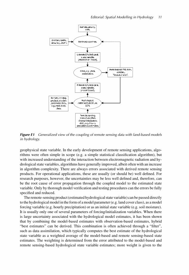
Remote sensing products are coupled to hydrological models in different ways. Theymight be used to drive the hydrological catchment model or a land surface model (LSM)directly or they might be combined with model-estimated geophysical state variable to pro-duce a “best estimate” via a filter. Figure E1 shows a generalized summary of the approach,which by no means covers all possibilities. Typically, remote sensing data are transformedinto an estimated hydrological state variable (product) via a retrieval algorithm that canuse physically based or empirical sub-models. Many algorithms are complex and requireancillary spatial data, such as topographical or meteorological data, to produce the required

PT1 WU088/Kelly March 1, 2004 8:9 Char Count= 0

Editorial: Spatial Modelling in Hydrology 11

Figure E1 Generalized view of the coupling of remote sensing data with land-based modelsin hydrology.

geophysical state variable. In the early development of remote sensing applications, algo-rithms were often simple in scope (e.g. a simple statistical classification algorithm), butwith increased understanding of the interaction between electromagnetic radiation and hy-drological state variables, algorithms have generally improved, albeit often with an increasein algorithm complexity. There are always errors associated with derived remote sensingproducts. For operational applications, these are usually (or should be) well defined. Forresearch purposes, however, the uncertainties may be less well defined and, therefore, canbe the root cause of error propagation through the coupled model to the estimated statevariable. Only by thorough model verification and testing procedures can the errors be fullyspecified and reduced.

The remote-sensing product (estimated hydrological state variable) can be passed directlyto the hydrological model in the form of a model parameter (e.g. land cover class), as a modelforcing variable (e.g. hourly precipitation) or as an initial state variable (e.g. soil moisture).It is usually only one of several parameters of forcing/initialization variables. When thereis large uncertainty associated with the hydrological model estimates, it has been shownthat by combining the model-based estimates with observation-based estimates, hybrid“best estimates” can be derived. This combination is often achieved through a “filter”,such as data assimilation, which typically computes the best estimate of the hydrologicalstate variable as a weighted average of the model-based and remote sensing-based stateestimates. The weighting is determined from the error attributed to the model-based andremote sensing-based hydrological state variable estimates; more weight is given to the

PT1 WU088/Kelly March 1, 2004 8:9 Char Count= 0

12 Spatial Modelling of the Terrestrial Environment

estimates with smaller associated error. A best estimate can be used to re-initialize thehydrological model at the next time step or it might also be used to initialize the remotesensing retrieval algorithm. While Toll and Houser (Chapter 12) demonstrate the use ofdata assimilation in LSMs, the development of data assimilation applications in hydrology,in general, is still in its infancy. For an account of its more mature application in theatmospheric sciences, Kalnay (2002) provides a good explanation of how data assimilationis used in numerical weather prediction. There are alternative filter methodologies that canbe used to combine observation-based and model-based estimates and these include spatialor temporal interpolation.

In the following four chapters different specific applications are described that coupleremote sensing with spatial hydrological models, in different ways. In Chapter 2, Bamberdescribes how the Antarctic ice sheet dynamics can be modelled, using satellite-derivedtopography estimates. In this example, the remote-sensing product is used as a drivingparameter in physically based models of ice flow. He shows that the accuracy of thealtimeter-based ice sheet elevation estimates affects the modelled estimates of ice flow,which is a key component in calculating the mass balance of Antarctica. The chapterby Kelly et al. (Chapter 3) analyzes and compares spatial variations of global ground-measured snow depth with satellite passive microwave estimates of snow depth. Sincesatellite estimates are areal in nature, while ground measurements tend to be representativeof a point, the spatial scaling between these types of estimates is uncertain. For example,how far are the point measurements representative of wider areal variations in snow depth?The chapter also summarizes recent and current approaches for satellite passive microwaveobservations of snow depth and SWE. Burke et al. (Chapter 4) demonstrate how coupledland surface and microwave emission models can help with the estimation of soil moisture.The chapter describes how passive microwave soil moisture estimates can be assimilatedinto a state-of-the-art land surface model (LSM). They recognize the shortcomings ofLSMs and suggest that improvements in model physics and improved parameterization ofsoil moisture heterogeneity in the pixels would improve the estimates of soil moisture and,therefore, improve the performance of the LSM. Finally, in Chapter 5, Bates et al. illustratehow high spatial resolution LiDAR and synthetic aperture radar (SAR) products can beused for flood inundation simulation. Interestingly, they suggest that the future of manyspatially distributed modelling frameworks will rely on remote sensing data, that are betterspecified in terms of the accuracy of the derived hydrological variable.

References

Anderson, M.G. and Bates, P.D., 2001, Model credibility and scientific enquiry, in M.G. Andersonand P.D. Bates (eds), Model Validation: Perspectives in Hydrological Science (Chichester: JohnWiley and Sons), 1–10.

Anderson, M.G. and Burt, T.P., 1985, Model strategies, in M.G. Anderson and T.P. Burt (eds),Hydrological Forecasting (Chichester: John Wiley and Sons), 1–13.

Beven, K.J., 2003, On environmental models of everywhere on the GRID, Hydrological Processes,17, 171–174.

Kalnay, E. 2002, Atmospheric Modeling, Data Assimilation and Predictability (Cambridge:Cambridge University Press).

Sherman, L.K., 1932, Streamflow from rainfall by unit-graph method, Engineering News Record,108, 501–505.