1*1 National Defense

Defence nationale

MULTIPATH MODELLING FOR TERRESTRIAL VHF RADIO DIRECTION FINDING (U)

by

William Read

^tcQio^m XMSP^OTEQ 8

Approved for public release; Distribution Unlimited

DEFENCE RESEARCH ESTABLISHMENT OTTAWA REPORT NO. 1300

Canada 19970115 057 December 1996 Ottawa

ABSTRACT

This report details the development of computer models to investigate and ex-

plain the effects of multipath on VHF radio direction finding (DF). The motivation for

this development was to help explain the large and small scale multipath effects which

occur for changes in transmitter and receiver position, or for changes in frequency. This is

particularly important when analyzing the capabilities of current wide and narrow band

DF methods, or when developing new DF methods. The development of the computer

models is based on representing the terrain and vegetation affecting the signal by a large

number of small (relative to the signal wavelength) isotropic reradiators. Polarization

effects are not accounted for. Although this kind of approach can quickly become a

computationally daunting task, a number of simplifications are introduced which greatly

simplify the calculations. Two examples have been included illustrating the use of the

proposed approach in the analysis and modelling of real world measurements.

RESUME

Le present rapport expose en details la conception de modeles informatiques

permettant Fexamenet l'explication des effets des trajets multiples sur la radiogoniometrie

VHF. Nous avons concu ces modeles dans le but de pouvoir expliquer les effets ä grande

et a petite echelle des trajets multiples qui se produisent lors de changements dans la

position de l'emetteur et du recepteur ou dans la frequence. Cela s'avere particulierement

important lors de l'analyse des capacites des methodes actuelles de radiogoniometrie de

bandes larges et restreintes ou dans le cadre de l'elaboration de nouvelles methodes. La

conception de ces modeles informatiques s'appuie sur la representation du relief et de la

vegetation affect ant le signal par un grand nombre de petites (par rapport ä la longueur

d'onde du signal) antennes isotropes de reemission. Nous n'avons pas rendu compte

des effets de polarisation. Bien qu'une teile approche puisse rapidement devenir une

täche computationnelle intimidante, nous avons incorpore certaines simplifications qui

facilitent grandement les calculs. Nous incluons deux exemples qui illustrent Putilisation

de l'approche proposee dans le cadre de l'analyse et de la moderation des mesures du

monde reel.

in

EXECUTIVE SUMMARY

Improvement of communications radio direction finding (DF) accuracy is a high

priority for the Canadian and Allied Forces. To this end, research in advanced DF tech-

niques has been carried out worldwide over the last two decades with the view of taking

advantage of advances in DF algorithms as well as the capabilities of modern processing

technology. At the Defence Research Establishment Ottawa (DREO), a series of field

trials were carried out to quantify the effects of multipath propagation during the Spring

of 1994. The field measurements were carried out using an experimental eight-channel

VHF DF system called the Osprey System.

In analyzing the field trial data it quickly became evident that the multipath

environment has a complex effect on the transmitter signal. To properly understand the

information yielded by the collected data, it was deemed necessary to develop computer

models so that multipath effects could be simulated under strict control - something that

is not possible in the real world.

The approach used to develop these computer models was to break the physical

environment into an immense grid of individual reradiating elements. Analogous to digi-

tizing an audio signal except using position (3-dimensions) instead of time (1-dimension).

A large part of the report deals with the development of this grid model, beginning with a

single reradiating element then analyzing the effect of collections of reradiating elements.

This includes an analysis of the effect of size and shape of the collection of reradiators on

an impinging signal, and the resultant reradiated signal. This is followed by an analysis

of the interaction between reradiator elements (i.e. mutual coupling) and finally the effect

of an infinite grid of reradiators (to represent the ground). Although the mathematics

become quite involved, the results agree with both the laws of physics and common sense

views of the real world - necessary conditions in order for a modelling approach to be

successful.

Given that the reradiating elements must be small in order to accurately repre-

sent features which cause multipath, the computational burden may increase prohibitively

as the number or size of these features increases. Consequently, this report also deals with

the appropriate simplifications that can be made to greatly reduce this computation bur-

den. These simplifications are somewhat dependent on the physical environment being

modelled, so that there are some cases where simplifications are not possible (i.e. very

uneven ground or very uneven vegetation requiring lots of individual features to be mod-

elled) so more work remains to be done in this area. However, for many real situations the

proposed simplifications can be employed with good success. To demonstrate this point,

two examples showing the simulation of measurements that have been made in the real

world have also been included.

The main benefit of the new approach is the ability to model various aspects

of the environment which will lead to a better understanding of the actual sources of

multipath, their numbers, and locations. This will allow the multipath environment to be

properly modelled for the purposes of testing DF methods and calibration techniques, as

well as open up the possibility of developing new methods which are capable of significantly

improving the accuracy of DF compared to current approaches.

VI

TABLE OF CONTENTS

Page

ABSTRACT/RESUME ui EXECUTIVE SUMMARY v TABLE OF CONTENTS vii LIST OF FIGURES ix

1.0 INTRODUCTION 1 1.1 The Modelling Approach 3 1.2 Further Considerations 5

2.0 MULTIPATH SOURCE CHARACTERISTICS 12 2.1 The Discrete Reradiator 12 2.2 Collections of Reradiators 14 2.3 Characterizing Multipath Sources 17 2.3.1 Beam Power 21 2.3.2 Beamwidth 21 2.3.3 Beam Phase 31 2.3.4 Reflections 31 2.3.5 The Beam Model 36

3.0 COUPLING EFFECTS 37 3.1 Coupling within a Multipath Source 37 3.2 Characteristics of a Coupled Multipath Source 41 3.2.1 Effect on Power 41 3.2.2 Effect on Beamwidth 45 3.2.3 Effect on Phase 45 3.2.4 Enhancement of Reflections 46 3.2.5 The Modified Beam Model 48 3.3 Processing for More Than One Multipath Source 48 3.3.1 Coupling between Multipath Sources 49 3.3.2 Internal Coupling 52 3.3.3 Comparing Coupling Methods 53

4.0 THE GROUND PLANE 63 4.1 The Ideal Ground Plane 63 4.2 Vegetation and Terrain Features 68 4.3 Variations in the Reradiation Properties 72

5.0 SUMMARY OF MULTIPATH EQUATIONS 78 5.1 Freespace Equations 79 5.2 Vegetation and Terrain Feature Equations 79 5.3 Nonhomogeneous Dielectric Earth Equations 80

vii

6.0 REAL WORLD MODELLING EXAMPLES 81 6.1 Example 1 81

6.2 Example 2 88

6.3 Assumption Verification . 90

7.0 CONCLUSIONS 93

REFERENCES REF-1

A.O CIRCULAR GROUND GRID CALCULATIONS A-l

vni

LIST OF FIGURES

Page

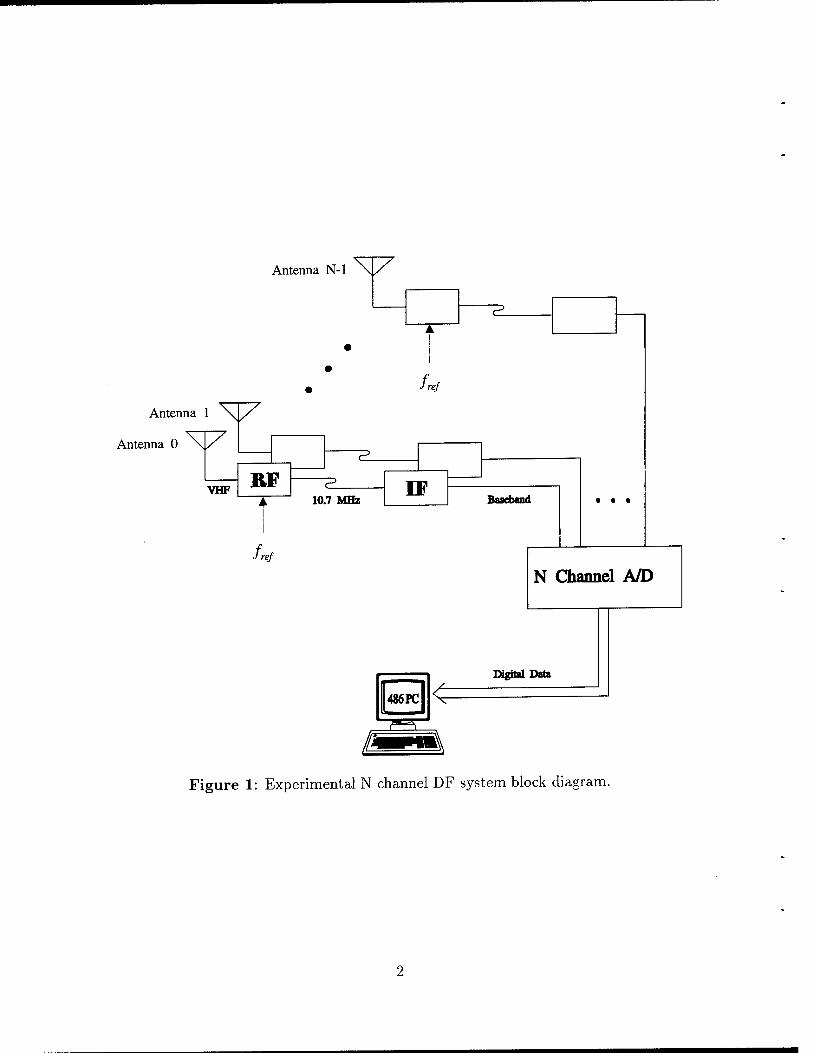
Experimental N channel DF system block diagram. 2

Signal power for a moving transmitter 6

Overview of a signal impinging on a large obstacle 8

Cartesian coordinate system representation for multipath source po-

sition 16

Geometry of simulation experiment to determine multipath source output as a function of receiver azimuth 18

Multipath signal power as a function of receiver azimuth angle for multipath line sources 19

Multipath signal phase as a function of receiver azimuth angle for multipath line sources 20

Vector representation of summation terms for a line source 23

Map showing phase contours as a function of position relative to the center of the multipath source 24

Geometry of line multipath source (open circles) and zero-phase line (dotted line) for # = 30° 26

Dumbbell multipath source showing (a) geometry and zero-phase line for <f>' = 27.2°, and (b) multipath power as a function of <j> 27

Dumbbell source vector diagram for <f>' = 27.2° 28

Bent cross multipath source showing (a) geometry and zero-phase line for <f>' = 43.2°, and (b) multipath power as a function of <j) 29

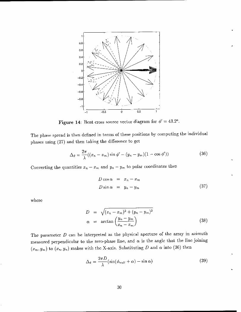
Bent cross source vector diagram for </>' = 43.2° 30

Multipath source main beam phase for the (a) line source, (b) dumb- bell, and (c) bent cross 32

Figure 16: Reflection beam generated by a line source for different orientations. 34

Figure 1:

Figure 2:

Figure 3:

Figure 4:

Figure 5:

Figure 6:

Figure 7:

Figure 8:

Figure 9:

Figure 10:

Figure 11:

Figure 12:

Figure 13:

Figure 14:

Figure 15:

IX

Figure 17: Comparison of the reflection beam generated by (a) a line source, (b) a thin rectangular shaped source, and (c) a thicker rectangular shaped 35 source.

Figure 18: Multipath source power (with coupling effects included) as a function of azimuth for the (a) line source, (b) dumbbell, and (c) bent cross. 39

Figure 19: Multipath source main beam phase (with coupling effects included) for the (a) line source, (b) dumbbell, and (c) bent cross 40

Figure 20: Maximum power for the line source as the reradiator spacing d is varied while n2

m is kept constant 42

Figure 21: Depiction of the first ten Fresnel zones for a transmitter and the kth

reradiator 44

Figure 22: Comparison of the reflection beam generated by (a) a line source, (b) a thin rectangular shaped source, and (c) a thicker rectangular shaped

47 source *'

Figure 23: Map used for simulation purposes and showing the geometry of the transmitter, receiver, and two multipath sources 54

Figure 24: Configuration of reradiators used to create a wall-like multipath source. 55

Figure 25: Relative amplitude of signal at receiver calculated using (a) the full coupling method, (b) the multipath source coupling method, and (c) the internal coupling method 56

Figure 26: Map of locations of transmitter, receiver, and multipath sources used in simulation to investigate effect of spacing 58

Figure 27: Mean squared error results for two approximate methods as a function of spacing between multipath sources 59

Figure 28: Map showing setup used for multipath simulation involving seven mul- tipath sources "1

Figure 29: Multipath simulation showing relative amplitude of signal at the re- ceiver calculated using (a) the full coupling method, (b) the multipath source coupling method, and (c) the internal coupling method. ... 62

Figure 30: Ideal ground plane showing direct and reflected signals 64

Figure 31: Geometry of a circular grid used for ground simulations 65

x

Figure 32: Results of ground simulation for ß = -1 showing the magnitude of the reradiator signals as a function of distance from the transmitter. 66

Figure 33: Above ground multipath source model. 68

Figure 34: Values of the coupling elements 7« as a function of the distance be-

tween reradiators rki • '5

Figure 35: Map showing site of multipath measurements carried out at DREO in

1994 82

Figure 36: Received signal power measured with respect to the transmitter posi-

tion 82

Figure 37: Shape of multipath sources showing reradiator positions for (a) small scatterer model, (b) tree model, and (c) large reflector model 84

Figure 38: Location of most significant multipath sources using (a) small scat- terer model, (b) tree model, and (c) large reflector model 86

Figure 39: Received signal power using (a) small scatterer model, (b) tree model, and (c) large reflector model 87

Figure 40: Map showing site of wideband DF measurements carried out at DREO

in 1992 89

Figure 41: Received signal power measured with respect to the transmitter fre-

quency 89

Figure 42: Received signal power using (a) tree model, and (b) large reflector

model 91

XI

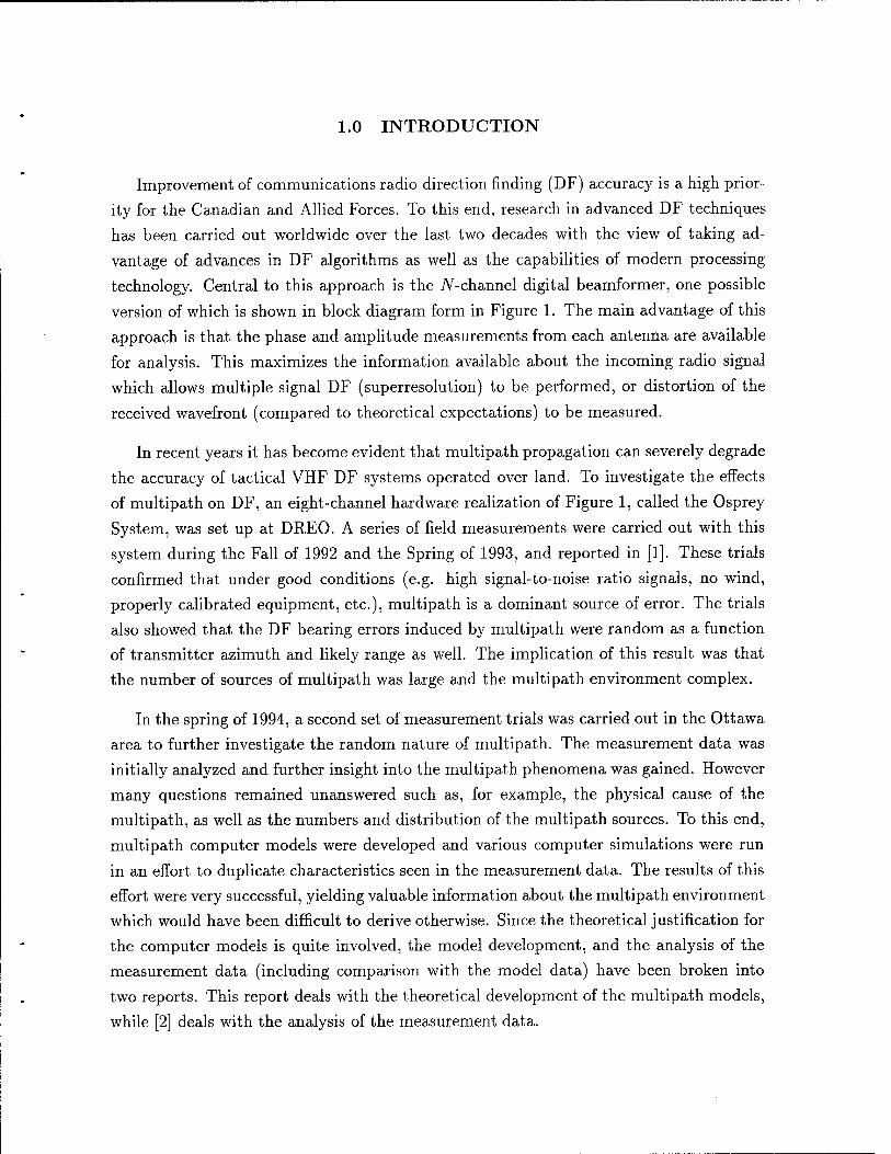
1.0 INTRODUCTION

Improvement of communications radio direction finding (DF) accuracy is a high prior-

ity for the Canadian and Allied Forces. To this end, research in advanced DF techniques

has been carried out worldwide over the last two decades with the view of taking ad-

vantage of advances in DF algorithms as well as the capabilities of modern processing

technology. Central to this approach is the iV-channel digital beamformer, one possible

version of which is shown in block diagram form in Figure 1. The main advantage of this

approach is that the phase and amplitude measurements from each antenna are available

for analysis. This maximizes the information available about the incoming radio signal

which allows multiple signal DF (superresolution) to be performed, or distortion of the

received wavefront (compared to theoretical expectations) to be measured.

In recent years it has become evident that multipath propagation can severely degrade

the accuracy of tactical VHF DF systems operated over land. To investigate the effects

of multipath on DF, an eight-channel hardware realization of Figure 1, called the Osprey

System, was set up at DREO. A series of field measurements were carried out with this

system during the Fall of 1992 and the Spring of 1993, and reported in [1]. These trials

confirmed that under good conditions (e.g. high signal-to-noise ratio signals, no wind,

properly calibrated equipment, etc.), multipath is a dominant source of error. The trials

also showed that the DF bearing errors induced by multipath were random as a function

of transmitter azimuth and likely range as well. The implication of this result was that

the number of sources of multipath was large and the multipath environment complex.

In the spring of 1994, a second set of measurement trials was carried out in the Ottawa

area to further investigate the random nature of multipath. The measurement data was

initially analyzed and further insight into the multipath phenomena was gained. However

many questions remained unanswered such as, for example, the physical cause of the

multipath, as well as the numbers and distribution of the multipath sources. To this end,

multipath computer models were developed and various computer simulations were run

in an effort to duplicate characteristics seen in the measurement data. The results of this

effort were very successful, yielding valuable information about the multipath environment

which would have been difficult to derive otherwise. Since the theoretical justification for

the computer models is quite involved, the model development, and the analysis of the

measurement data (including comparison with the model data) have been broken into

two reports. This report deals with the theoretical development of the multipath models,

while [2] deals with the analysis of the measurement data.

Antenna N-l

fref

Antenna 1

Antenna 0

VHF RF ■p.

e_ T 10.7 MHz

IF

/, ref

486 PC

?=r

Baseband

N Channel AID

Digital Data

Figure 1: Experimental N channel DF system block diagram.

1.1 The Modelling Approach

The normal approach taken in propagation modelling is to estimate the expected

values for the received signal based on modelling the surface using either known shapes or

statistical surfaces (i.e. rough surfaces). For example, successive ridges along the signal

path could be modelled using knife-edge diffraction techniques [3]. These approaches are

often successful at predicting the average path loss as a function of transmitter position

(i.e. the average path loss for the transmitter moved to various positions over a given

area) but cannot predict fine-scale effects (i.e. the change in path loss as the transmitter

is moved distances on the order of one meter). In this analysis, it is the fine-scale effects

and the statistical nature of these effects which are of the most interest.

The failure of most propagation models to predict fine-scale effects is a function of

the requirement for these models to provide useful information (i.e. expected path loss)

without being too difficult to use. Consequently the constructive and destructive phase

effects of competing signal paths are usually ignored to simplify processing. It is these

phase effects which give rise to the fine-scale multipath effects.

Exact multipath effects could probably be modelled using approaches employed by

electromagnetic software packages such as the Numerical Electromagnetics Code (NEC).

However, these packages are normally used to predict antenna characteristics so that for

the scale of the problem described here, the computer processing and memory require-

ments would be prohibitive. Additionally, exact sizes, positions, electrical properties of

everything surrounding the signal path would have to be measured. Consequently, trying

to model exact effects would not be practical.

The approach employed in this report is to break the terrain, or parts of the terrain,

into very small pieces with dimensions on the order of a fraction of a wavelength. Each

part can then be considered as a secondary or elemental reradiating source which, in

turn, can be modelled in a very simple way. This is similar in most respects to Huygens'

principle [4], and analogous to using digital signal processing to analyze analog signals.

To simplify the analysis, a number of assumptions and simplifications have been made.

These include:

1. the transmit and receive antennas are isotropic,

2. refractive effects due to variations in air density are insignificant

3. vertical polarization only is considered, and

4. de-polarization effects can be ignored.

Of these assumptions, ignoring de-polarization effects has the greatest impact in the

results. Including these effects would provide additional accuracy to the modelling but at

the expense of considerably complicating the analysis, which is not considered warranted

in this case.

Despite these assumptions and simplifications, the approach of subdividing the terrain

still remains computationally intensive. For example, modelling the ground between the

transmitter and receiver for ranges of several kilometers would require using an extremely

large number of elemental reradiators which then becomes a daunting computational

task. Consequently, rather than try to solve the entire multipath environment in this

way, various simplified environments were explored which either allowed using a more

manageable number of reradiators, or could be handled in a very computationally efficient

way. From these explorations, analytical approaches were developed which could then be

used to represent the simplified environments. More complex environments could then be

represented by combining a number of these analytical approaches.

Central to the development of these analytical approaches is a proper understanding

of their eventual intended purpose. This provides the basis for deciding which approxi-

mations can be made for the sake of computational simplicity, and which cannot. In this

report, the main purpose for the development of the analytical approaches is to provide

a better understanding of the various mechanisms which give rise to multipath, and to

be able to produce a simulated environment which mimics the effects observed in the real

world. There was no intention to be able to exactly predict real world results.

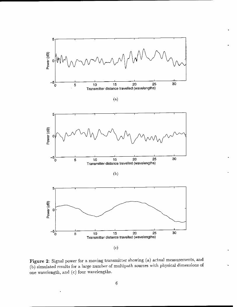
To illustrate the intended purpose, Figure 2a provides a measurement sample taken

from multipath field trials described [2]. The measurement was taken from an experiment

where a transmitter broadcast a CW signal at 62.5 MHz while slowly moving along a

straight line. The receive system, called Osprey, was located approximately 2 km away

from the transmitter in a position where the direct signal path was roughly perpendicular

to the route followed by the transmitter. Figure 2a shows the received signal amplitude

as a function of the distance travelled by the transmitter. Figure 2b is a simulation

using the same transmitter-receiver geometry and assuming a large number of multipath

sources (based on the model developed in Section 4.2) with dimensions on the order of

one wavelength (4.8 meters). Figure 2c uses the same model but assumes the average

dimensions are on the order of five wavelengths. Although neither of the two simulated

results exactly duplicate the actual result, Figure 2c better mimics the ripple behavior

of the actual measurements, particularly in terms of the higher frequency content of the

ripple, providing evidence that a significant portion of multipath was generated by objects

with dimensions closer to one wavelength than four wavelengths.

An important assumption that was also used to produce simpler analytical expressions

was the assumption that for terrestrial signal paths investigated in [2], large numbers of

objects were typically involved in the production of multipath. This is based on field trial

results, as discussed in Section 1.0, and visual surveys. Visually, the number of objects

known to cause multipath that were scattered in and around the signal paths used in field

trials was large (e.g. trees, bushes, fences, buildings, etc. - see [6] for a more extensive

list of objects which cause multipath). Although not definitive proof, these observations

suggest that assuming a large number of multipath sources is a very safe bet.

The advantage of this assumption is that since multipath is considered the result

of contributions from a large number of objects, the characteristics that are the most

important are the characteristics resulting from this collection of objects. The exact

characteristics of each multipath source are then less important, and it is therefore only

necessary to identify the most important characteristics which contribute to the collective

effects.

1.2 Further Considerations

Before getting into a detailed mathematical analysis, it is useful to describe in more

detail how the modelling with isotropics elements is done, and the limitations of this

approach. To understand the approach that has been taken, it is useful to consider two

simplifying examples of the real world environment. In the first example, the transmitter

and receiver are on the ground and a few kilometers apart, the terrain is very flat, and

the vegetation consists of scattered groves of trees and bushes. The signal arriving at the

receiver will consist of the direct signal, plus a signal reflected off the ground as well as

signals scattered off the vegetation. Since the ground is flat, it will likely be homogeneous

(i.e. its electrical characteristics are the same everywhere), with the result that the ground

reflected signal will be well behaved. In this case the ground could easily be modelled as a

simple reflection plane. For the vegetation, a single tree or bush could be approximately

modelled by a single large isotropic element, or more accurately modelled by subdividing

10 15 20 25 Transmitter distance travelled (wavelengths)

30

(a)

10 15 20 25 Transmitter distance travelled (wavelengths)

30

(b)

CD

CD

o 0.

10 15 20 25 Transmitter distance travelled (wavelengths)

30

(c)

Figure 2: Signal power for a moving transmitter showing (a) actual measurements, and (b) simulated results for a large number of multipath sources with physical dimensions of

one wavelength, and (c) four wavelengths.

6

the tree or bush into smaller parts and then modelling each part by separate appropriately

sized isotropic elements.

In the second example, the transmitter and receiver are again a few kilometers apart,

but vegetation is nonexistent and the ground is rolling. In this case the ground signal is

not just a simple reflection, but reflections off many different parts of the ground. For

modelling purposes, the ground surface itself is subdivided into many small sections, each

section is then modelled by a suitably chosen isotropic element. The result is a huge grid

of isotropic elements with elevation features identical to the actual ground.

Once the model has been setup, the next step is to compute the signal reradiated from

each element. This requires solving for the signal incident on each isotropic element as

the reradiated signal is directly proportional to this incident signal, or

S reradiated P^incident \*-)

where ß is the complex reradiation coefficient. The electromagnetic field would be related

to these signals according to

s = fie (2)

where s represents either the incident or reradiated signal, /J,2 is the collection area of

the isotropic element, and e is the corresponding electric field. A similar real-world

example would be the electrically short dipole which has a similar behaviour to an isotropic

element, although its reradiation pattern is not isotropic. In the real-world example, the

signals srera<nated and sincident would correspond to voltages setup in the antenna, \i would

correspond to the length of the antenna, and ß would be related to the mismatch between

antenna and freespace impedances.

Determining the incident signal for each isotropic element provides the greatest dif-

ficulty in this modelling approach, but once it has been done, the signal arriving at the

receiver is simply the sum of the contributions from each source. For a receiving system

consisting of an array of antennas, this summation would need to be done for each an-

tenna. (Note that the calculation of the incident signals for each isotropic element need

only be done once, however, irrespective of the number of receiving antennas).

Two obvious features of the isotropic model are the parameters ß and /?, whose choice

will obviously affect the value of the reradiated signals. Since /i3 will be directly propor-

tional to the volume of the physical object being modelled, it's determination is relatively

straightforward. The choice of ß would ideally be based on the electrical properties of

7

the object being modelled as well, however, no attempt has been made to explore this

relationship. This is because in many cases a value of ß = -1 is sufficient for modelling

purposes, and where this value is not appropriate, a better value can be derived by com-

paring real data with simulation data and then adjusting ß to get the best match. If the

adjustment approach is used, simple logic can also be applied to ensure the values of ß

make sense.

9 0 8 0 o c So ' 0 0 0 0 e .t ■',° 0 0 0 0

i 0 M " 0 0 •

k ! < : i I I ' I I | I I transmitter , | , j f I , ' M »I '.IIMl r+Transmitter . ' I ' « fl ! U

-80 -60 -40 -20 0 20 40 X coordinate (meters)

60 80

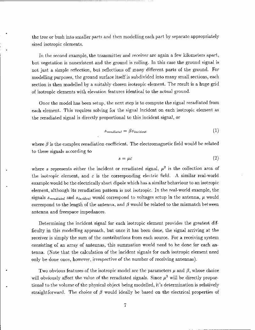
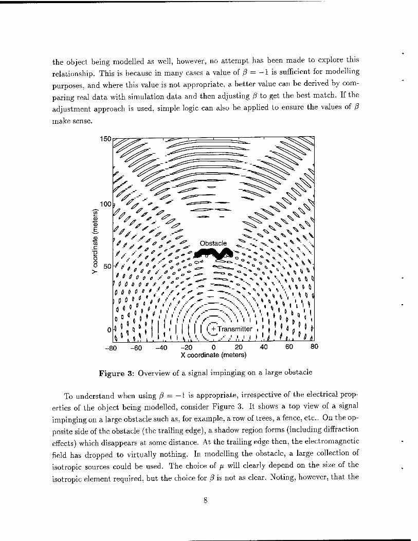
Figure 3: Overview of a signal impinging on a large obstacle

To understand when using ß = -1 is appropriate, irrespective of the electrical prop-

erties of the object being modelled, consider Figure 3. It shows a top view of a signal

impinging on a large obstacle such as, for example, a row of trees, a fence, etc.. On the op-

posite side of the obstacle (the trailing edge), a shadow region forms (including diffraction

effects) which disappears at some distance. At the trailing edge then, the electromagnetic

field has dropped to virtually nothing. In modelling the obstacle, a large collection of

isotropic sources could be used. The choice of fj. will clearly depend on the size of the

isotropic element required, but the choice for ß is not as clear. Noting, however, that the

electromagnetic field is near zero on the trailing edge then any isotropic element located

on this edge will meet the condition

£reradinted ~T~ ^incident ~ " V /

which is equivalent to

S reradiated "T Sincident ~ " V /

Given the relationship between the incident and reradiated signals (1) then

(1 + ß)Sincident ~ 0 (5)

which leads to ß « -1 assuming \sincident\ > 0. If \sincident\ ~ 0 the choice of ß is

unimportant, i.e. choosing ß = — 1 is still reasonable.

Letting ß = — 1 will not be appropriate for all situations. On the other side of the

obstacle in Figure 3 (on the side incident to the transmitter signal - the leading edge), a

value of ß = — 1 would result in a strong reflection, i.e. the obstacle would act like a bumpy

reflector. However, if the obstacle absorbs some of the signal energy (e.g. conversion to

heat energy - induced currents in the obstacle could cause ohmic heating) then the signal

reflection would be weaker than expected. In this case it is more appropriate to use

a smaller value for \ß\. Additionally, the dielectric constant of the obstacle will affect

the phase of the reflected signal which results in ß taking on an imaginery component.

Obviously in the reflection case it is more accurate to try and determine ß from measured

data, although ß = — 1 provides a reasonable starting point.

The major failing of the isotropic element model is the inability to accurately model

losses. For example a perfectly matched dipole will not produce any reflected signal. A

shadow zone will still be setup since the dipole has extracted power from the incoming

signal (i.e. the electric field signal is converted to an electrical signal). In the case of the

isotropic element, there is no such mechanism to convert the incoming signal to another

form of energy, only a mechanism to redirect the signal flow. This flaw could be overcome

by changing the antenna pattern so that it is no longer isotropic. However, this introduces

considerable complications to the analysis which were not considered warranted given the

main purpose of the modelling discussed in this report.

To justify the last point, consider the fact that the main effects of a multipath source

can be classified as shadowing or reflection. For a single multipath source, these two

mechanisms are mutually exclusive from the perspective of the receiver (i.e. the receiver

9

can be affected by shadowing or reflection, but not both simultaneously). For multipath

sources located between the transmitter and receiver, and near the signal path (ignoring

the ground for the moment), shadowing will be the dominant mechanism, so that for

modelling purposes ß = -1 is suitable. This results in strong reflected signals for the

modelled multipath sources, but since these reflections will generally propagate in direc-

tions away from the receiver they will be of little importance. It is possible that multiply

reflected signals could be directed towards the receiver, but these effects will be minor

and can also be ignored.

Outside this shadow region, reflections are more likely to be the dominant mechanism.

In this case, the choice of ß will be made by comparing simulations with real measure-

ments, as discussed previously, and will incorporate the effect of losses. In the case of

high losses the choice of ß may no longer be appropriate for the shadows, but since these

shadows will be directed away from the receiver, this error is not important.

In the case of the ground, reflections will be very important regardless of location. For

a flat ground with varying dielectric properties, reflection will be the only mechanism so ß

is chosen accordingly (if ß ^ -1 this will result in a signal below the surface, but since the

receiver is above the surface, this signal can be ignored). For a ground which is not fiat,

both reflections and shadowing are possible mechanisms. For this, modelling is restricted

to the case where the elevation varies but the surface is perfectly reflecting (ß = -1). In

other words, terrain with both varying electrical characteristics and varying elevation is

not addressed, although the effects could reasonably be inferred from the ground models

that are developed in this report.

One final comment regarding the definition of multipath used in this report. The

general definition used here is

S multipath — ^receiver ^ideal \ /

In the freespace case, the ideal signal is the direct transmitter to receiver signal. In this

case, multipath will be the signal that is reradiated, reflected, etc., by objects around the

signal path. In the terrestrial case, the definition for the ideal signal used in this report

is slightly different. Since all terrestrial signal paths will involve ground reflections, the

ideal terrestrial signal is defined as the signal that occurs when the ground is perfectly

flat and perfectly reflecting. Mathematically,

sideal == ^direct ~r ^reflected \ )

10

Although the ideal ground reflected signal is technically a multipath signal, for terrestrial

problems the ground reflected signal is inescapable so that the above definition is more

analytically useful.

In the rest of this report, many of the discussions become embroiled in complex math-

ematical derivations. Given the rather random nature of the real world, and that the

aim of this research to emulate but not duplicate real world effects, it might at first seem

that the mathematics becomes unnecessarily involved. However, the detail is required

in order to establish the theoretical underpinnings of the models, their limitations, and

when various simplifying assumptions are justified.

To this end, a major portion of this report focuses on developing the mathematical

theory of the isotropic model in a slow and determined manner. The development of the

model may at first seem a little detached from the real-world, however this is necessary in

order to examine and understand the various aspects of the model in more detail. At the

end of this development, simulation examples are provided to illustrate how the various

models and modelling approaches can be applied to real world problems.

The rest of this report is divided into six main parts. In Section 2.0, the isotropic rera-

diator in freespace is introduced, followed by an examination of a collection of reradiators

in freespace. Based on this examination, size of the multipath source is shown to be an

important characteristic, while shape is found to be relatively less important except when

reflections occur. In Section 3.0, the effects of coupling are examined. Since the inclusion

of coupling effects dramatically increases the computational requirements of modelling,

ways of reducing the computations are also discussed. In Section 4.0, the effects of the

ground on path loss and coupling are examined. This examination includes vegetation

and terrain effects, as well as the effect of a nonhomogeneous ground. In Section 5.0, the

models introduced in the three previous sections are summarized and their limitations

noted. In Section 6.0, two examples are provided illustrating how the models could be

used to investigate and better understand effects observed in real-world measurements.

Finally, in Section 7.0, the concluding remarks are presented.

11

2.0 MULTIPATH SOURCE CHARACTERISTICS

In this part, multipath sources are modelled by dividing the source up into elemental

isotropic reradiators. The discussion starts with the introduction of a simple mathematical

model of a single elemental reradiator in freespace and its affect on a transmitter signal.

This model is then evolved to include the effects of a collection of elemental reradiators

in freespace. Using these collections to represent various shaped multipath sources, the

characteristics of multipath sources are then analyzed and discussed. In presenting the

effects of shape, shapes are limited to simple two-dimensional geometric shapes for conve-

nience, however, the analysis could be easily extended to include real world objects such

as bushes, trees, buildings, etc.

2.1 The Discrete Reradiator

In this section, the equations which describe the behaviour of an isotropic reradiating

element are derived. Since these reradiators first receive an external signal which is

subsequently retransmitted, it is useful to consider the receive response of the reradiator

first.

For a radiating isotropic source in freespace, the radio wave expands in a spherical

wave with the source at the center. Using an optics approach, the power extracted by a

receiving antenna at a distance r can be computed by considering the area of the spherical

wave intercepted by the antenna compared to the total area 4?rr2 of the spherical wave.

The received power will be given by,

P - p P (8) rrcvr — 1 tx . 9 V /

where PTCVr is the received signal power, Ptx is the power radiated by the transmitter, //2

is the effective collecting area of the receiving antenna, and it is assumed 47rr2 > //2.

The complex amplitude sTCVT of the received signal can also be related to that of the

amplitude of the transmitted signal stx using the fact that \s\ oc P* (where s and P

represent signal amplitude and power respectively) and the phase delay is a function of

the path length r. This leads to the result

s = til (-V-) e~l2-fr (9) r \Zy/TTj

12

where it is again assumed that 47rr2 > p2 or equivalently r > \ij2\pK.

If the condition on r is not met, nearfield effects begin to affect the results and the

above equations may be considered approximations only. In the extreme case where r <

HJIypK, the above expressions break down completely since they predict that |src„r| > \six\

and Prcvr > Ptx which clearly makes no sense. In reality, to satisfy the law of physics,

nearfield effects will ensure that the relationship \srcvr\ < \stx\ is always true. The exact

nature of these nearfield effects will be dependent on the actual object being modelled

(i.e. its shape, electrical properties, etc.) but can be approximated by

— Stxt -j 2^r r ^ P A for r < -^ (10)

More realistic nearfield equations have been tested but were found to have no effect on

the results presented in this report.

Expressions (9) and (10) can by represented by the more general expression

Srcvr = Stxp{r) (H)

where p(r) is called the freespace attenuation function in this report and represents the

effect of path length on both amplitude and phase of the signal. For a discrete reradiator

in freespace, the attenuation function is given by

Pair) = <

P _7-22tr .„ . P z 3 xr it r>

2^ " 2V? (12)

~J \T otherwise

where the subscript a has been added to identify it as the freespace attenuation function.

The corresponding path loss is given by \pa(r)\2. Other forms of the attenuation function

(i.e. attenuation over a reflecting ground) are discussed in Sections 4.2 and 4.3.

If the receiving element is a reradiator, the above expression can be modified slightly

to yield

^incident = Stxpam(ra) V-1-"/

where pam{-) is the freespace attenuation expression for the transmitter-reradiator path

using p? = p?m for the collection area of the reradiator, and ra is the range from the

transmitter to the reradiator.

13

Once the signal has been received, it is reradiated. This can be introduced into the

model by incorporating a complex reradiation coefficient ß such that \ß\ < 1. The rera-

diated signal sm measured at the reradiator will then be

Sm = StxßPam{ra) (14)

The portion of the reradiated signal that arrives at the receiver can be determined by

applying (13) to (14). Since this will be the multipath signal, the final result is given by,

Smult = stxßpam(ra)par(rb) (15)

where par(-) is the freespace attenuation expression for the reradiator-receiver path using

H2 = p* for the collection area of the receiving antenna, and rb is the range from the

reradiator to the transmitter. A distinction has made between par(-) and pam{-) since

the collecting areas of the reradiating elements and the receiving antenna (fi2m and p?r

respectively) may be different.

For simplicity, the receiving antenna is treated as matched as well as isotropic (i.e.

the size of the antenna is chosen so that no special matching network would be required).

Under these conditions the effective collecting area is given by [7]

47T Ä = f- (16)

2.2 Collections of Reradiators

A number of useful characteristics can be derived by simulating the effects of more

complex multipath sources using a collection of isotropic sources. The received multipath

signal will then be the sum of all the individual contributors

N

Smult — ^Smultk \^V k=\

where N is the total number of reradiators making up the multipath source and the

subscript k is used to distinguish the contribution from individual reradiators. Applying

(15) to each reradiator yields

N

I k-1

Smult = Stxß J2 Pam(rak)par(rbk) (18)

14

The assumption is made here that the multipath source is homogeneous (its electrical

properties are the same everywhere) so that ß is the same for all the reradiators. Nonho-

mogeneous multipath sources can be modelled by breaking the source into small enough

parts that each part is homogeneous.

To simplify later derivations, it is useful to redefine the path lengths ra and rb as the

distance from the transmitter to the center of the multipath source and the distance from

the center of the multipath source to the receiver, respectively. A reference signal can

then be defined as

sref= sixpam(ra)por(rb) (19)

Additionally further simplifications result if ra,rb > Dmax where Dmax is the largest

physical dimension of the multipath source. In this case \pam(rak)\ ~ \pam{ra)\ and

\par(rbk)\ ~ \Par{n)\ with the result that (18) can be rewritten as

N

I k-1

SmuU = STe}ßYJ^2-f(rak-ra+rbk'rb) (20)

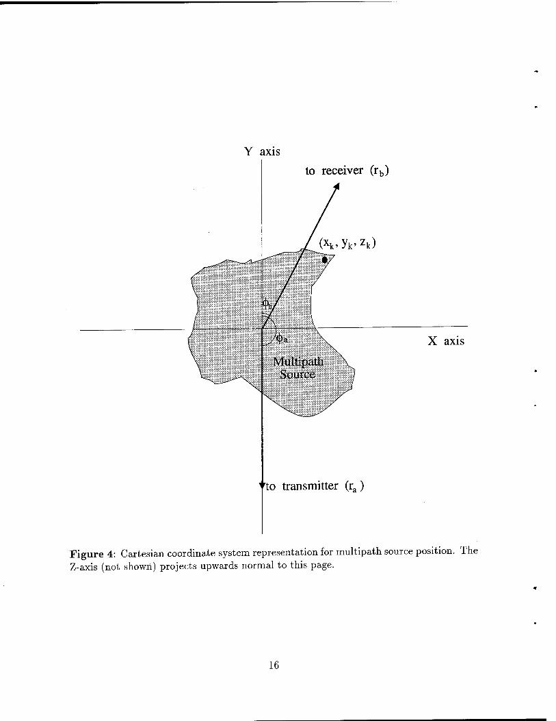
Using the Cartesian coordinate system shown in Figure 4, where the origin corresponds

to the center of the multipath source, then the following approximations can be used

rak ~ ra - (zfc sin </>a cos ^>a + ykcos<f>acosipa + zksinipa)

Hk ~ rb-(xk sin <j)b cos ipb + yk cos (j)b cos ißb +zk sin ipb) (21)

where </>a and (j)b are the transmitter and receiver direction angles measured on the X-Y

plane with respect to the X-axis, and i\)a and ipb are the corresponding direction angles

measured with respect to the Z-axis. Without loss of generality, the X-Y plane is assumed

to be oriented so that the transmitter lies on the negative Y-axis (cj)a = 180° and i\)a =

0°) as shown in the figure. Defining <j> = <j>h and iß = ißb, and using the preceding

simplifications, (20) becomes

N

k=l

Since, in terrestrial applications, the X-Y plane will generally be approximately parallel

to the ground, then <j> and ip are respectively called the azimuth angle and the elevation

angle (of the receiver) here.

15

Y axis

to receiver (rb)

(xk, yk> zk)

Multipath Source }

<m ̂m

to transmitter (r )

X axis

Figure 4: Cartesian coordinate system representation for multipath source position. The Z-axis (not shown) projects upwards normal to this page.

16

2.3 Characterizing Multipath Sources

Various characteristics can be inferred from (22), however, before performing any

further mathematical manipulations, it is useful to first examine some simulation results

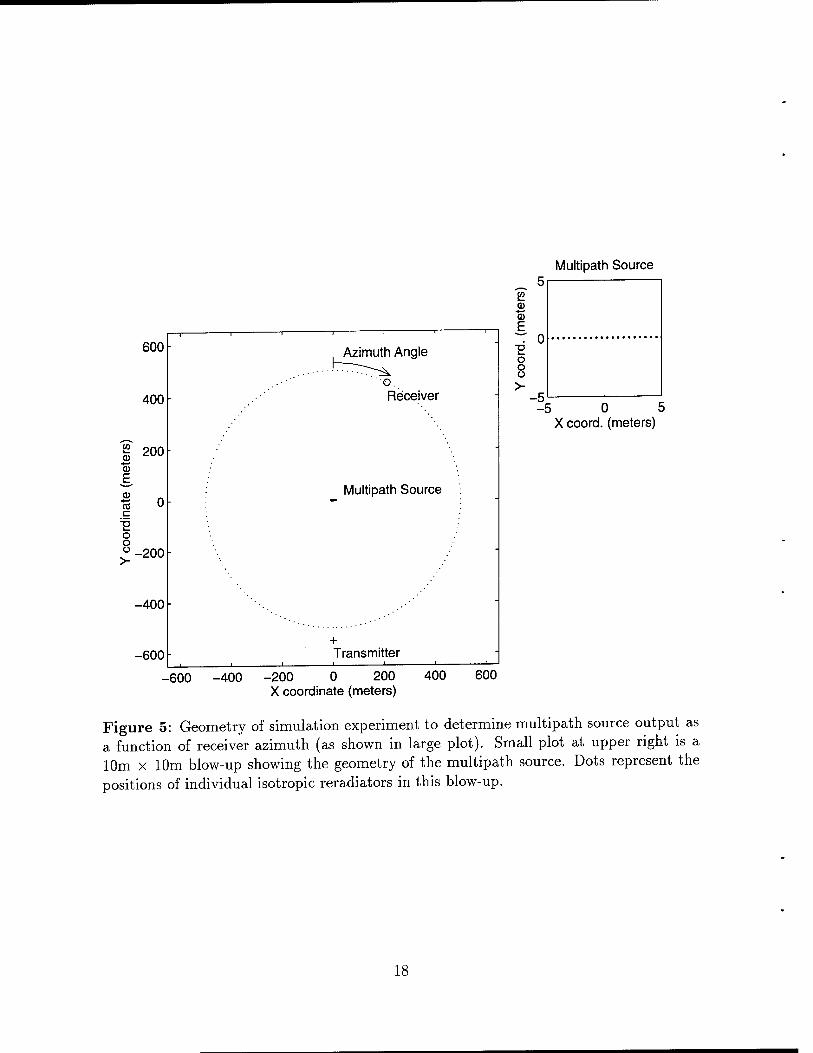
in order to provide an idea of which characteristics are the most important. Figure 5 shows

the geometry of a simulation experiment carried out using (18). In this experiment the

receiver was moved in a circle around a multipath source while the transmitter position

was kept fixed. The transmitter, receiver, and multipath source were all placed on the

X-Y plane. The multipath source consisted of a linear array of N = 10 reradiators (see

blow-up in the upper right hand corner of the figure) where the spacing d between adjacent

reradiators was chosen to be a small fraction of a wavelength, namely, d = 0.1A m. Since

coupling effects are not taken into account here, \im was chosen so that each reradiator

represents a contiguous area, neither overlapping nor spread apart. This leads to fim = d.

Using a transmitter frequency of 62.5 MHz, then A = 4.8 m and d = \i = 0.48 m. A value

of ß = — 1 was also chosen.

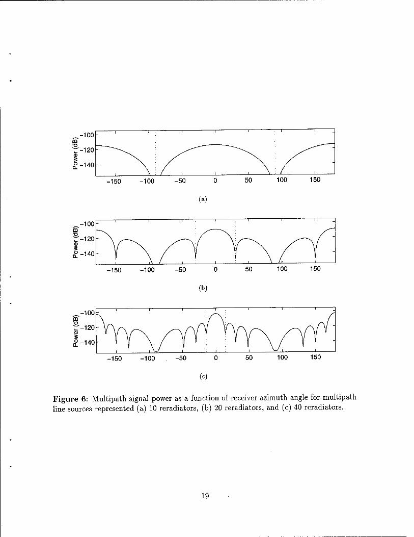
Figure 6a shows the power of the multipath signal measured as a function of the

receiver azimuth angle. Figure 6b shows the received power for the same experiment

except using a line array of 20 reradiators with the same spacing, while Figure 6c shows

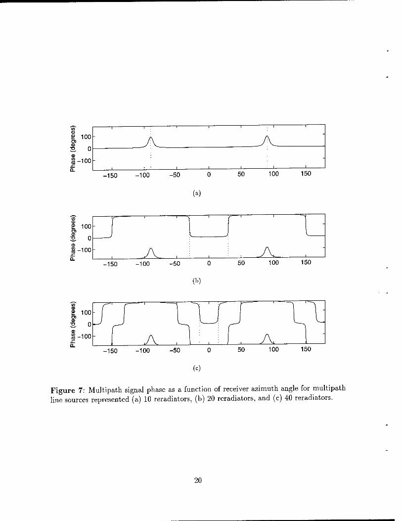
the received power for a line array of 40 reradiators (also with the same spacing). Figure 7

shows the corresponding received signal phases measured relative to sref/ß (i.e. the phase

of the summation term in (20).

Examining the three cases shown in Figures 6 and 7 the outputs have a lobed struc-

ture (where adjacent lobes are separated by nulls) with the two largest lobes lying in

the directions 0° and 180°. In this report, the lobe at 0° is called the main beam and

would correspond to the electromagnetic shadow cast by the multipath source. Lobes of

comparable power (such as the one at 180°) but in different directions are called reflection

beams. In beamformer terminology, the remaining lobes are called sidelobes while in op-

tics they are called diffraction lobes. In any case, since most of the multipath power will

be concentrated in the main and reflection beams, most of the multipath effects observed

by the receiver will be due to these two beams. Hence characterizing these beams goes

a long way towards providing an effective means of characterizing the most important

features of a multipath source. To this end, the maximum power of the main beam, its

beamwidth, and the phase variation across the beam are investigated in detail in Sections

2.3.1-2.3.3, while the corresponding characteristics of the reflection beam are dealt with

in Section 2.3.4. Finally, in Section 2.3.5 the general notation used in this report for the

17

Multipath Source

52

<D E

03

600 , 1

400

200

0

-200

-400

-600 ■ * t

Azimuth Angle

Receiver

Multipath Source

Transmitter

-600 -400 -; 200 0 200 X coordinate (meters)

400 600

0 5 X coord, (meters)

Figure 5: Geometry of simulation experiment to determine multipath source output as a function of receiver azimuth (as shown in large plot). Small plot at upper right is a 10m x 10m blow-up showing the geometry of the multipath source. Dots represent the positions of individual isotropic reradiators in this blow-up.

18

-150 -100

(a)

-150 -100

(b)

-150 -100

(c)

Figure 6: Multipath signal power as a function of receiver azimuth angle for multipath line sources represented (a) 10 reradiators, (b) 20 reradiators, and (c) 40 reradiators.

19

a> 8> 100|-

® B 0

Jg -100

-150 -100 -50 50 100 150

(a)

Pha

se (

degr

ees

o

o

o

o o

- 1 i

-150 -100 -50 50 100 150

(b)

-150 -100 100 150

(c)

Figure 7: Multipath signal phase as a function of receiver azimuth angle for multipath line sources represented (a) 10 reradiators, (b) 20 reradiators, and (c) 40 reradiators.

20

multipath source model is introduced.

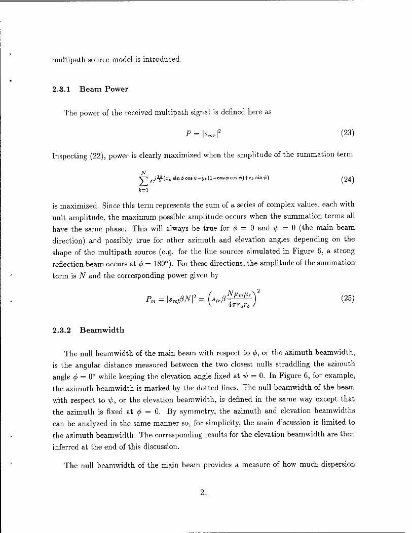
2.3.1 Beam Power

The power of the received multipath signal is defined here as

P=\Smr\2 (23)

Inspecting (22), power is clearly maximized when the amplitude of the summation term

N V"> j2Z-(xksm4>cosip-yk(l-cos(f>cosil>)+zksmil>) ^Z^)

is maximized. Since this term represents the sum of a series of complex values, each with

unit amplitude, the maximum possible amplitude occurs when the summation terms all

have the same phase. This will always be true for <f> = 0 and ip = 0 (the main beam

direction) and possibly true for other azimuth and elevation angles depending on the

shape of the multipath source (e.g. for the line sources simulated in Figure 6, a strong

reflection beam occurs at </> = 180°). For these directions, the amplitude of the summation

term is N and the corresponding power given by

Pm = \SrefßNf=Lxß^^)2 (25) V 4:7rrarb J

2.3.2 Beamwidth

The null beamwidth of the main beam with respect to <f>, or the azimuth beamwidth,

is the angular distance measured between the two closest nulls straddling the azimuth

angle <j> = 0° while keeping the elevation angle fixed at t/> = 0. In Figure 6, for example,

the azimuth beamwidth is marked by the dotted lines. The null beamwidth of the beam

with respect to if;, or the elevation beamwidth, is defined in the same way except that

the azimuth is fixed at (j> = 0. By symmetry, the azimuth and elevation beamwidths

can be analyzed in the same manner so, for simplicity, the main discussion is limited to

the azimuth beamwidth. The corresponding results for the elevation beamwidth are then

inferred at the end of this discussion.

The null beamwidth of the main beam provides a measure of how much dispersion

21

occurs in the reradiating beam (the greater the beamwidth the greater the dispersion and

the lower the power that is redirected towards the receiver). The nulls occur when sm = 0

which, in azimuth, corresponds to

N

I y eix(**sin0-i/*U-«»*)) _ o (26)

where the fact that $ = 0° was used. The solution to the above expression can be

determined geometrically by representing each summation term as a unit vector on the

complex plane. For <f> = 0, these vectors are all aligned with the real axis, as illustrated

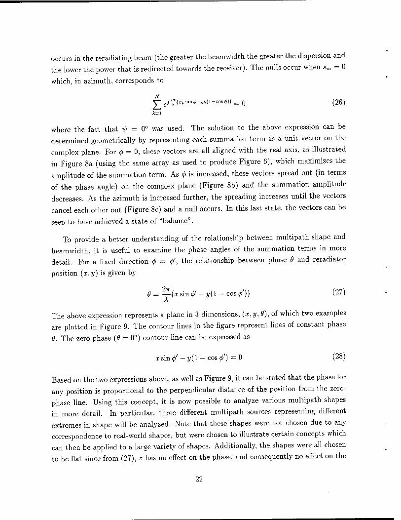
in Figure 8a (using the same array as used to produce Figure 6), which maximizes the

amplitude of the summation term. As </> is increased, these vectors spread out (in terms

of the phase angle) on the complex plane (Figure 8b) and the summation amplitude

decreases. As the azimuth is increased further, the spreading increases until the vectors

cancel each other out (Figure 8c) and a null occurs. In this last state, the vectors can be

seen to have achieved a state of "balance".

To provide a better understanding of the relationship between multipath shape and

beamwidth, it is useful to examine the phase angles of the summation terms in more

detail. For a fixed direction </> = (/>', the relationship between phase 0 and reradiator

position (x,y) is given by

6 = ^{x sin <t>'-y(l-cos </>')) (27)

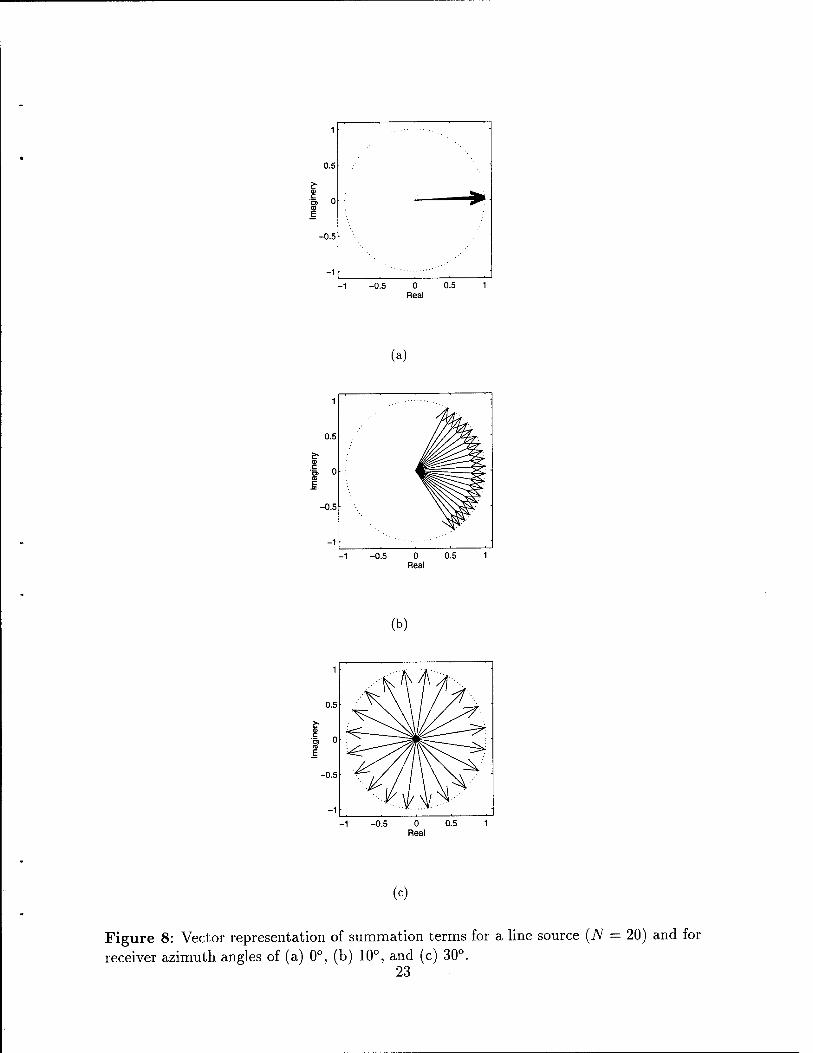
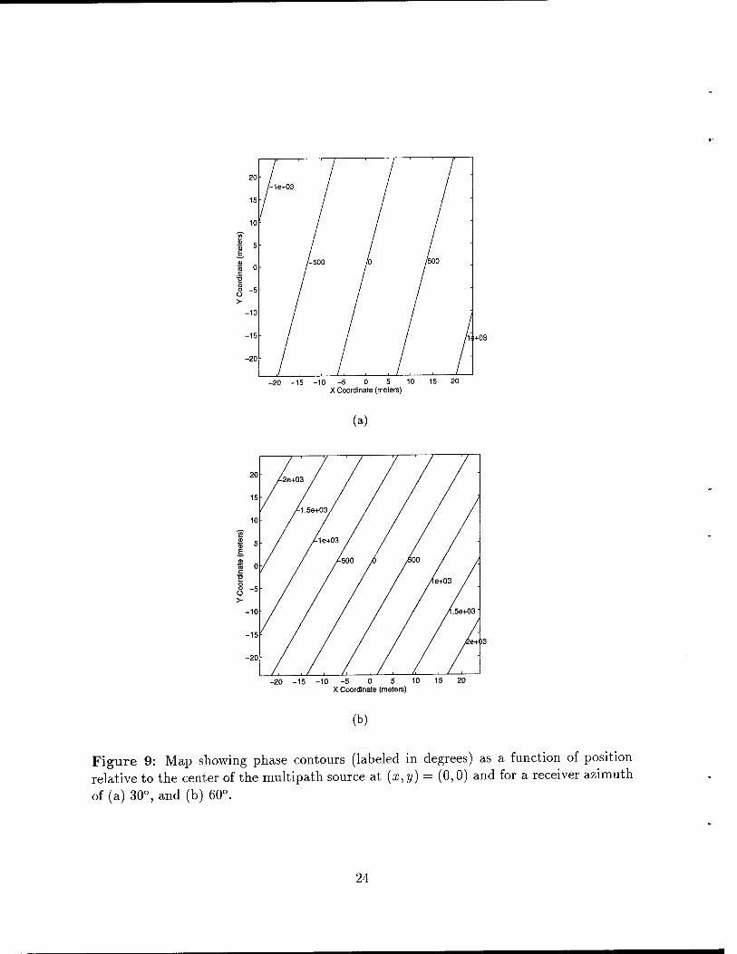
The above expression represents a plane in 3 dimensions, (x, y, 9), of which two examples

are plotted in Figure 9. The contour lines in the figure represent lines of constant phase

0. The zero-phase (0 = 0°) contour line can be expressed as

xsm<f>'-y(l-coB<l>') = 0 (28)

Based on the two expressions above, as well as Figure 9, it can be stated that the phase for

any position is proportional to the perpendicular distance of the position from the zero-

phase line. Using this concept, it is now possible to analyze various multipath shapes

in more detail. In particular, three different multipath sources representing different

extremes in shape will be analyzed. Note that these shapes were not chosen due to any

correspondence to real-world shapes, but were chosen to illustrate certain concepts which

can then be applied to a large variety of shapes. Additionally, the shapes were all chosen

to be flat since from (27), z has no effect on the phase, and consequently no effect on the

22

(a)

(b)

•& o

(c)

Figure 8: Vector representation of summation terms for a line source (N = 20) and for receiver azimuth angles of (a) 0°, (b) 10°, and (c) 30°.

23

20 /-1e+03

/

15 /

/

10 / /

"ST S 5 E.

ra 0 c

o 8 -5

/-500 r /500

> -10

/ / -15

/ / -20

( , /■

-20 -15 -10 -5 0 5 10 15 20 X Coordinate (meters)

(a)

-20 -15 -10 -5 0 5 10 15 20 X Coordinate (meters)

(b)

Figure 9: Map showing phase contours (labeled in degrees) as a function of position relative to the center of the multipath source at (x, y) = (0,0) and for a receiver azimuth

of (a) 30°, and (b) 60°.

24

azimuth beamwidth (it would, however, effect the elevation beamwidth).

The first shape is again the line source example. Figure 10a shows a case with N = 20

with the zero-phase line drawn for <f>' = 30°. This particular receiver azimuth corresponds

to the main beam null marked by the dotted line in Figure 10b. It is quite evident that

the perpendicular distance from the zero-phase line to consecutive reradiators varies in

a linear manner. This will be true regardless of the orientation of the line source or the

direction </>'. To achieve a state of balance as discussed previously, the phases must be

evenly spread through 360° as in Figure 8c. This leads to the result

N — 1 Ae — 2TT——— radians (29)

where A# is the difference between the maximum and minimum reradiator phase, or

Ae = max{6>o,..., 0jv-i} - min{0o, —, &N-I} (30)

with 0k representing the phase of the kth reradiator. In the real world, multipath sources

are generally continuous which can best be modelled as N —> oo. Hence for a continuous

line source

A# = 2% radians (31)

The above expression will also be true for any shape which is uniformly distributed with

respect to the zero-phase line of a main beam null.

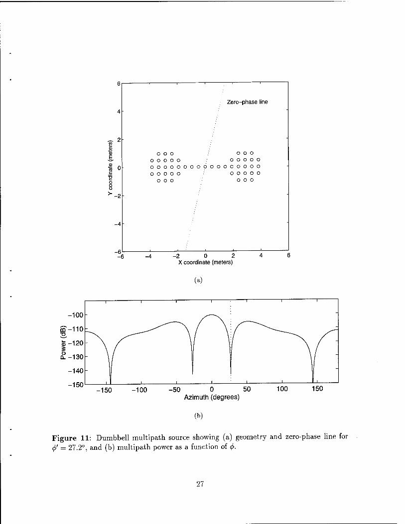
The second shape to be considered is the dumbbell shown in Figure 11a. The zero-

phase line for <f>' = 27.2° has also been drawn. This receiver bearing corresponds to the

main beam null marked by the dotted line in Figure lib. From the relationship of the

zero-phase line to the position of the reradiators, it is possible to predict that the phases of

the summation terms will be non-uniformly spread with the phases concentrated towards

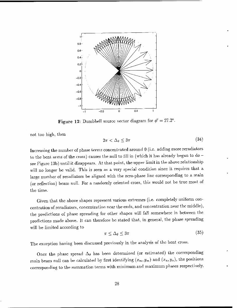
the minimum and maximum values. This is verified by the vector diagram shown in

Figure 12 with two groups of phase terms centered around phase angles of approximately

—7r/2 and 7r/2. In this case, the total spread in the balanced state will be less than for

the line source but still great enough that balancing can occur (i.e. the minimum spread

will be 7r). Therefore, for a multipath source with the main reradiation near the ends and

away from the zero-phase line,

7T < Ae < 2TT (32)

The concentration of the phase angles about —w/2 and 7r/2 corresponds to the two con-

centrations of reradiators at opposite ends of the dumbbell shape. The farther apart the

25

-2 0 2 X coordinate (meters)

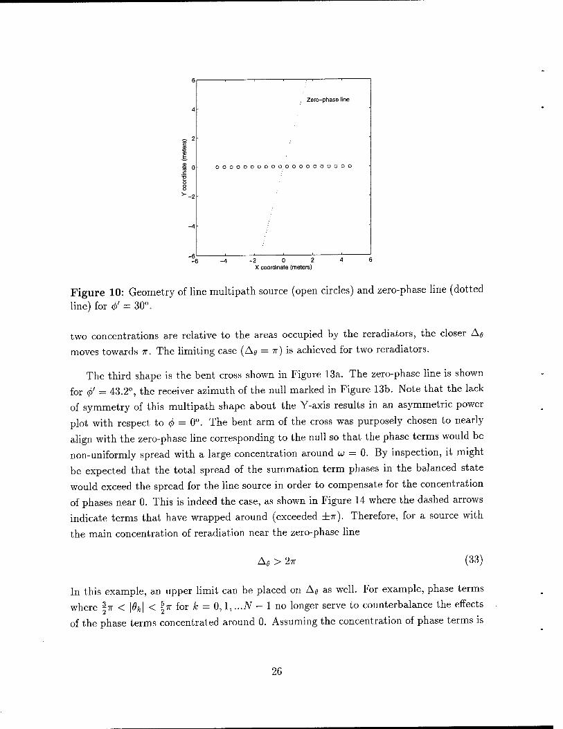
Figure 10: Geometry of line multipath source (open circles) and zero-phase line (dotted

line) for <f>' = 30°.

two concentrations are relative to the areas occupied by the reradiators, the closer Ae

moves towards w. The limiting case (Ae = n) is achieved for two reradiators.

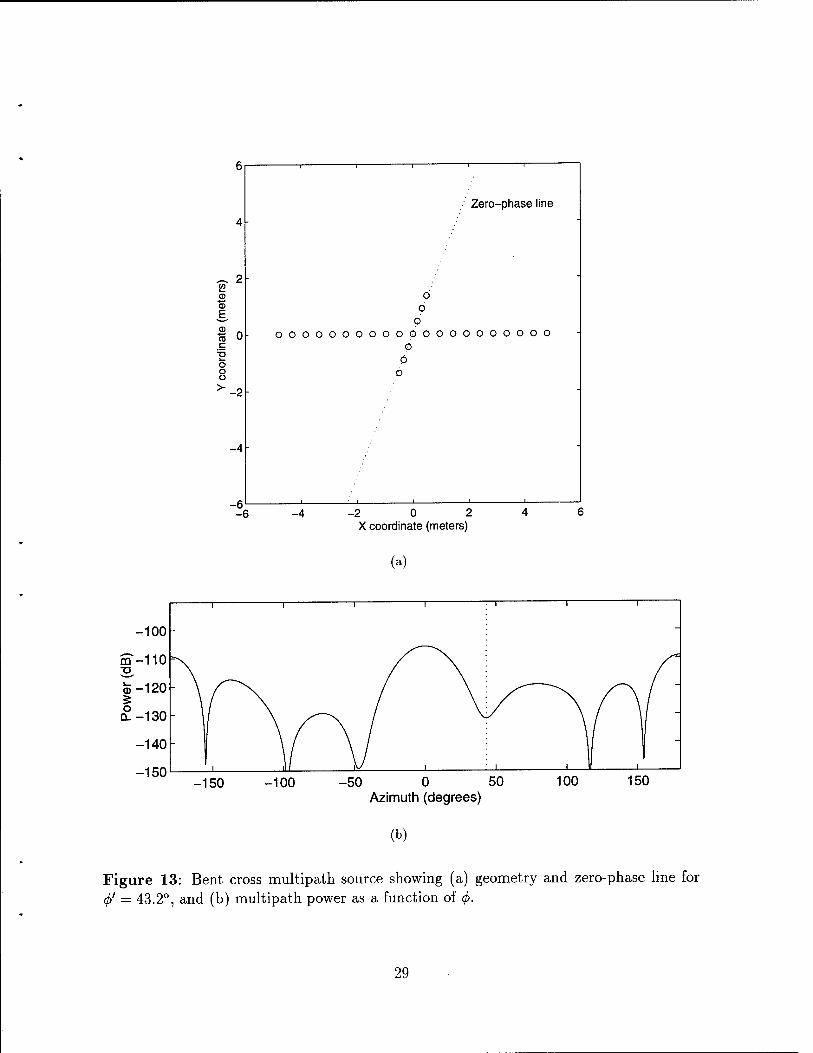
The third shape is the bent cross shown in Figure 13a. The zero-phase line is shown

for </>' = 43.2°, the receiver azimuth of the null marked in Figure 13b. Note that the lack

of symmetry of this multipath shape about the Y-axis results in an asymmetric power

plot with respect to <f> = 0°. The bent arm of the cross was purposely chosen to nearly

align with the zero-phase line corresponding to the null so that the phase terms would be

non-uniformly spread with a large concentration around w = 0. By inspection, it might

be expected that the total spread of the summation term phases in the balanced state

would exceed the spread for the line source in order to compensate for the concentration

of phases near 0. This is indeed the case, as shown in Figure 14 where the dashed arrows

indicate terms that have wrapped around (exceeded ±r). Therefore, for a source with

the main concentration of reradiation near the zero-phase line

A« > 2TT (33)

In this example, an upper limit can be placed on Ae as well. For example, phase terms

where -7r < \6k\ < §7r for k - 0,1, ...N - 1 no longer serve to counterbalance the effects

of the phase terms concentrated around 0. Assuming the concentration of phase terms is

26

4-

~ 2 tn i— CD *-< CD

E.

cS 0

o o CJ

Zero-phase line

o o o o o o ooooo ooooo ooooooooooooooooo ooooo ooooo

o o o o o o

-6 -4-2 0 2 X coordinate (meters)

(a)

-150 -100 -50 0 50 Azimuth (degrees)

100 150

(b)

Figure 11: Dumbbell multipath source showing (a) geometry and zero-phase line for <f)' = 27.2°, and (b) multipath power as a function of <j>.

27

1 •KA'A'Ä/IU-

0.8 'f[

0.6 Will// /' 0.4 \NNNN\^\I III/// / S^'

0.2 ^111 W///^^^^/ • " V^>^ \

0 f^\^^ ^ -0.2 /w/fll BJ^ON. ^~~~~~~-~-^\ : "

-0.4 //y///l\\ l\\\\\\ ^W -0.6 ' ■ Ijj/J//l\\\ l\\\\\\ \\ -0.8 '^m 1 mÄAt\ 'iTiOwv sKA .■■'

-1 ■ 'Ywyy/yfy

-0.5 0.5

Figure 12: Dumbbell source vector diagram for <j>' = 27.2°.

not too high, then 2TT < Ae < 3TT (34)

Increasing the number of phase terms concentrated around 0 (i.e. adding more reradiators

to the bent arms of the cross) causes the null to fill in (which it has already begun to do -

see Figure 13b) until it disappears. At that point, the upper limit in the above relationship

will no longer be valid. This is seen as a very special condition since it requires that a

large number of reradiators be aligned with the zero-phase line corresponding to a main

(or reflection) beam null. For a randomly oriented cross, this would not be true most of

the time.

Given that the above shapes represent various extremes (i.e. completely uniform con-

centration of reradiators, concentration near the ends, and concentration near the middle),

the predictions of phase spreading for other shapes will fall somewhere in between the

predictions made above. It can therefore be stated that, in general, the phase spreading

will be limited according to 7T < Ae < 3TT (35)

The exception having been discussed previously in the analysis of the bent cross.

Once the phase spread Ae has been determined (or estimated) the corresponding

main beam null can be calculated by first identifying (xm,ym) and (xn,y„), the positions

corresponding to the summation terms with minimum and maximum phases respectively.

28

^ 2

£

to 0 c

T3 i_ O o o

-2

-6

Zero-phase line

o o

o oooooooooopoooooooooo

0 0

D

-2 0 2 X coordinate (meters)

(a)

-150 -100 -50 0 50 Azimuth (degrees)

100 150

(b)

Figure 13: Bent cross multipath source showing (a) geometry and zero-phase line for <j)' = 43.2°, and (b) multipath power as a function of (j>.

29

1

0.8

0.6

0.4

0.2 \M^. 0

0.2 ^0f^\^' U.4

0.6

0.8

-1 m V^

-0.5 0.5

Figure 14: Bent cross source vector diagram for <j)' = 43.2°.

The phase spread is then defined in terms of these positions by computing the individual

phases using (27) and then taking the difference to get

Ae = y((x„ - xm) sin <f>' - (y„ - ym)(l - cos </>'))

Converting the quantities xn - xm and yn - ym to polar coordinates then

(36)

D cos a = xn — xT

Ds'ma = yn — y„ (37)

where

D = y/{xn - xm)2 + (yn - ymy yn 2/m

a — arctan Xn %m

(38)

The parameter D can be interpreted as the physical aperture of the array in azimuth

measured perpendicular to the zero-phase line, and a is the angle that the line joining

(xm,ym) to (xn,yn) makes with the X-axis. Substituting D and a into (36) then

Ae = —:— (sm((f)nuii + a) - sin a) A

(39)

30

and finally rearranging in terms of <f>nuu results in

\2-KD Ul = arcsm + sin a a (40)

Using the minimum and maximum values for Ae to calculate the minimum and max-

imum values of <f>nuu for the main beam null, and noting that the null beamwidth will be

twice these values of <f>, then

arcsm 2D

+ sin a] —a < hw < 2 . /3A . \

arcsm I —— + sin a I — a (41)

In the realworld, large multipath sources (D > A) will usually have both width and depth

(relative to the transmitted signal direction) so that a « 0. Under these conditions the

expression above simplifies to

^ < hw < ~ (42)

The most notable thing in either expression is that as D increases the beamwidth de-

creases. Therefore the smaller the multipath source, the greater the scattering of the

reradiated signal.

As mentioned previously, the above analysis also applies to the elevation beamwidth

ipbw except that the X and Z axes are interchanged. The main effects on the results is that

the X coordinates of the reradiators constituting a multipath source will have no effect

on the elevation beamwidth, and D will be the elevation aperture.

2.3.3 Beam Phase

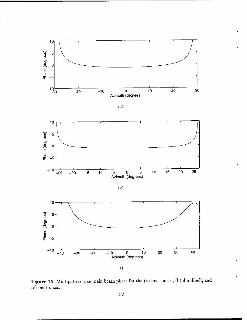
Figure 15 shows the phase (measured relative to sref/ß) of the three representative

multipath sources described in the previous section. Only receiver azimuth angles corre-

sponding to the main beam are shown. In all three cases the phase is well behaved, being

zero at <j> = 0° and gradually changing as a function </> until near the beam edges where

it changes more rapidly.

2.3.4 Reflections

Up to this point, the analysis of multipath source shape and size has been restricted

31

-10 0 10 Azimuth (degrees)

30

(a)

-25 -20 -15 -10 -5 0 5 Azimuth (degrees)

10 15

(b)

-40 -30 -20 -10 0 10 Azimuth (degrees)

20

(c)

Figure 15: Multipath source main beam phase for the (a) line source, (b) dumbbell, and

(c) bent cross.

32

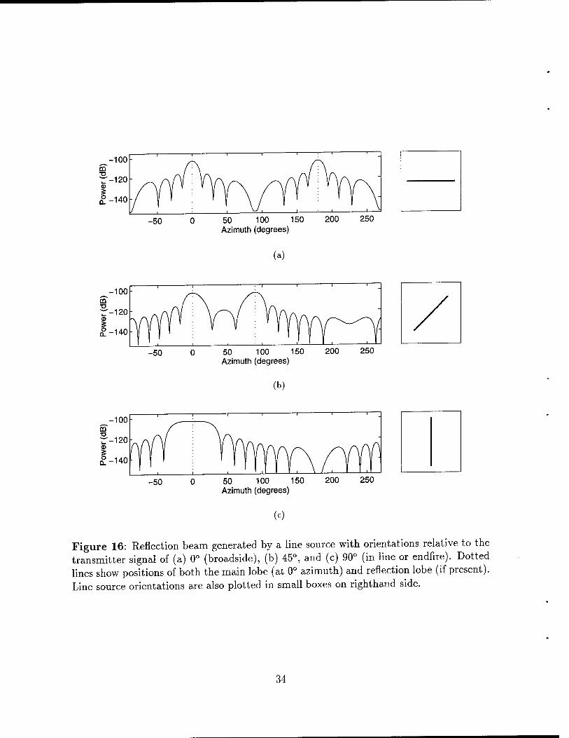
to the characteristics of the main beam. In general, this analysis is also applicable to

the reflection beam except that the shape of a multipath source and its orientation has

a pronounced effect on the direction and power of the reflection beam. In the linear

source case, for example, the electrical symmetry of the array along the length of the

line source dictates that the main beam will be duplicated symmetrically about a line

running the length of the line source. This second beam is defined here as a reflection

beam. Examples are shown in Figure 16 for three orientations of the line source. For the

0° and 45° orientations, the center of the reflection lobes correspond to 180° and 90° in

azimuth, respectively. For the 90° orientation the line source is aligned with the signal

direction so that the main and duplicate beams become one and the same.

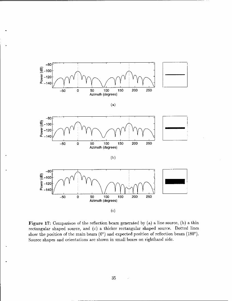
Figure 17 shows a comparison between the reflection beam generated by a line source,

a rectangular shaped source, and a square shaped source. As has already been implied,

in the case of the line source, the amplitude of the reflection beam is the same as the

main beam. In the case of the thin rectangular shaped source (three rows of reradiators),

the reflection beam is still generated although lower in amplitude than the main beam.

Finally, in the case of the thicker rectangular shaped source (ten rows of reradiators),

there is no obvious reflection beam.

Two important points are illustrated by these examples. The first is that reflection

beams tend to be generated if the multipath source is thin with respect to the direction of

the transmitted signal. In the case of the thick rectangle, a signal is reflected backwards

from each row of reradiators, but since the signals from different rows travel different

distances, these signals tend to cancel each other. For example, a signal reflected off the

first row and the k row will have a phase difference of

»,, = ^ (43)

If the distance between the two rows is (k — \)d = A/4 the two signals will cancel. Hence

for a strong reflection beam "thin" means less than A/4.

The second point is that since the mechanism that generates the reflection beam is

similar to the main beam, the preceding analysis can be applied. The only difference is

that the direction of the reflection beam will be different from <j> = 0 (by definition) and

the apparent value of the reradiation constant for the reflection beam (ßr) may be lower

(i.e. ßr < ß).

33

-100 00

-^ 120

I 1 1 — 1 I —i 1—

CD

£-140

-50 0 50 100 150 Azimuth (degrees)

200 250

(a)

-50 50 100 150 Azimuth (degrees)

200 250

(b)

-50 50 100 150 Azimuth (degrees)

200 250

(<0

Figure 16: Reflection beam generated by a line source with orientations relative to the transmitter signal of (a) 0° (broadside), (b) 45°, and (c) 90° (in line or endfire). Dotted lines show positions of both the main lobe (at 0° azimuth) and reflection lobe (if present). Line source orientations are also plotted in small boxes on righthand side.

34

S-100

-50 50 100 150 Azimuth (degrees)

200 250

(a)

-80

3-100

1-120

I 1 1 I 1 ' 1 1 i

o °--140

i I t

' 1 \

-50 50 100 150 Azimuth (degrees)

200 250

(b)

§§-100

-50 50 100 150 Azimuth (degrees)

200 250

(c)

Figure 17: Comparison of the reflection beam generated by (a) a line source, (b) a thin rectangular shaped source, and (c) a thicker rectangular shaped source. Dotted lines show the position of the main beam (0°) and expected position of reflection beam (180°). Source shapes and orientations are shown in small boxes on righthand side.

35

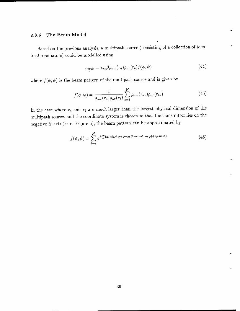
2.3.5 The Beam Model

Based on the previous analysis, a multipath source (consisting of a collection of iden-

tical reradiators) could be modelled using

Smuit = stxßpam{ra)paT(rb)f{(f>,ip) (44)

where f{4>,iß) is the beam pattern of the multipath source and is given by

1 N

/(</>, %j)) = ^ J^T £ Pam(rak)par(nk) (45) Pam\ra)Par{rb) j.=l

In the case where ra and rb are much larger than the largest physical dimension of the

multipath source, and the coordinate system is chosen so that the transmitter lies on the

negative Y-axis (as in Figure 5), the beam pattern can be approximated by

N

I k=\

f(± i\ _ ST" J2f{xksm4>cosi>-yk{'V-cos4>cosip)+zksmilj) UQ\

36

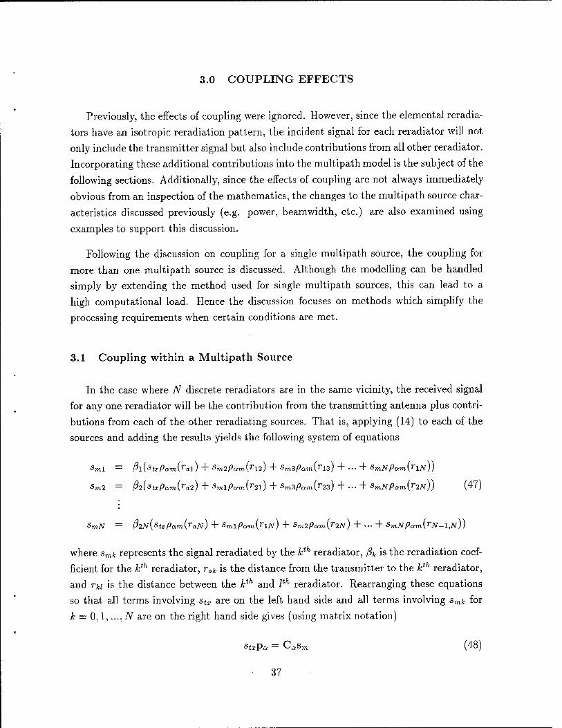
3.0 COUPLING EFFECTS

Previously, the effects of coupling were ignored. However, since the elemental reradia-

tors have an isotropic reradiation pattern, the incident signal for each reradiator will not

only include the transmitter signal but also include contributions from all other reradiator.

Incorporating these additional contributions into the multipath model is the subject of the

following sections. Additionally, since the effects of coupling are not always immediately

obvious from an inspection of the mathematics, the changes to the multipath source char-

acteristics discussed previously (e.g. power, beamwidth, etc.) are also examined using

examples to support this discussion.

Following the discussion on coupling for a single multipath source, the coupling for

more than one multipath source is discussed. Although the modelling can be handled

simply by extending the method used for single multipath sources, this can lead to a

high computational load. Hence the discussion focuses on methods which simplify the

processing requirements when certain conditions are met.

3.1 Coupling within a Multipath Source

In the case where JV discrete reradiators are in the same vicinity, the received signal

for any one reradiator will be the contribution from the transmitting antenna plus contri-

butions from each of the other reradiating sources. That is, applying (14) to each of the

sources and adding the results yields the following system of equations

■5ml = ßl(StxPam(ral) + Sm2Pam(ri2) + Sm3Pam(ri3) + ... + SmN Pamirs))

Sm2 = 02{stxpam(ra2) + smipam(r2i) + smzpam(r2z) + ... + smNpam(r2N)) (47)

SmN = ß2N(stxpam(raN) + Smipam(riN) + Sm2pam(r2N) + ••• + SmJV/w(nV-l,Jv))

where smk represents the signal reradiated by the kth reradiator, ßk is the reradiation coef-

ficient for the kth reradiator, rak is the distance from the transmitter to the kth reradiator,

and Vki is the distance between the kth and Ith reradiator. Rearranging these equations

so that all terms involving stx are on the left hand side and all terms involving smk for

k = 0,1,..., N are on the right hand side gives (using matrix notation)

StxPa = Casm (48)

37

where pa is the TV x 1 vector representing the attenuations from the transmitter to each of

the reradiators (stxpa represents the incident signal) with elements p1,p2,...,PN defined

by Pk = -Pam(rak) (49)

sm is the TV x 1 vector representing the reradiated signal with elements sml,sm2, ...,smjv,

and Ca is the N x N coupling matrix with elements

cki = Pam(rki) for k^l, fc,/ = l,2,3,...,/V (50)

and

ckk = ^ (51) Pk

The solution for the reradiated signals can be determined by solving the system of

equations represented by (47), or by rearranging (48) to get

Sm = StxC^Pa (52)

Finally, the received multipath signal will be the sum of all the reradiated signals with

the appropriate corrections made for the losses incurred over the reradiator to the re-

ceiver paths. To represent this mathematically, the reradiator-receiver attenuations are

represented by the iV x 1 vector qa whose elements qu q2,..., qN are defined by

qk = par(nk) (53)

where rbk represents the distance from the kth reradiator to the receiver. The multipath

signal at the receiver is then given by

Smult = StxC&C^Pa (54)

This is called the freespace multipath expression in this report. For a single reradiator

this expression reduces to (15).

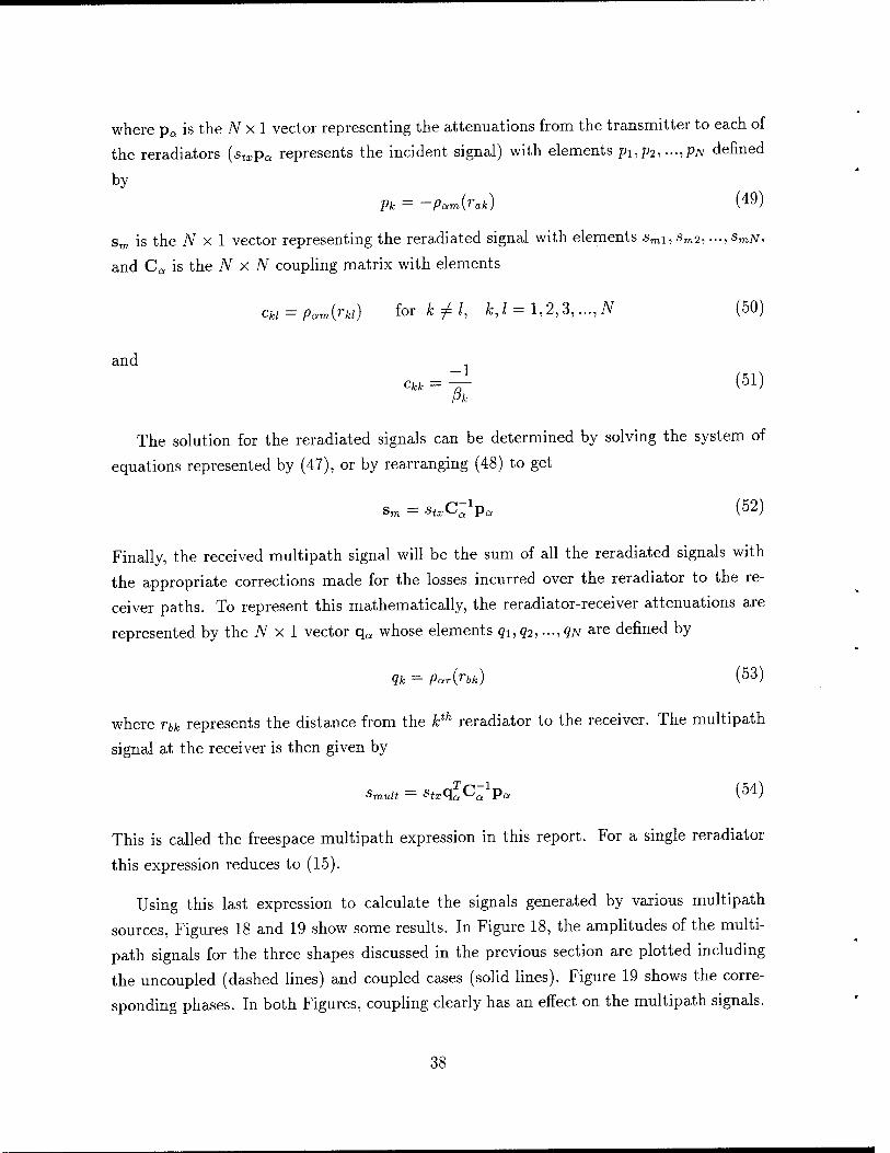
Using this last expression to calculate the signals generated by various multipath

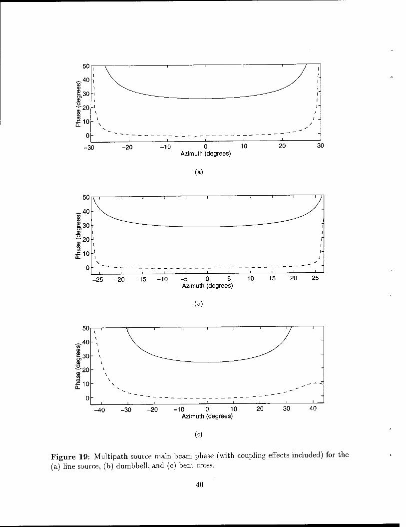
sources, Figures 18 and 19 show some results. In Figure 18, the amplitudes of the multi-

path signals for the three shapes discussed in the previous section are plotted including

the uncoupled (dashed lines) and coupled cases (solid lines). Figure 19 shows the corre-

sponding phases. In both Figures, coupling clearly has an effect on the multipath signals.

38

-150 -100 -50 0 50 Azimuth (degrees)

100 150

(a)

-100

I \ -T I 1 r I

m-110

S3-120

£-130

^ \

> / * / If

y

- ~~ — —■

\ If

V

-140 l|

i i i

-150 -100 -50 0 50 Azimuth (degrees)

100 150

(b)

-100

-150 -100 -50 0 50 Azimuth (degrees)

100 150

(c)

Figure 18: Multipath source power (with coupling effects included) as a function of azimuth for the (a) line source, (b) dumbbell, and (c) bent cross.

39

-30 -20 -10 0 10 Azimuth (degrees)

20

(a)

-25 -20 -15 -10 -5 0 5 10 Azimuth (degrees)

15 20

(b)

-40 -30 -20 -10 0 10 Azimuth (degrees)

20 30 40

(c)

Figure 19: Multipath source main beam phase (with coupling effects included) for the (a) line source, (b) dumbbell, and (c) bent cross.

40

3.2 Characteristics of a Coupled Multipath Source

In many ways the derived characteristics of a multipath source are very similar when

coupling effects are taken into account as when they are ignored. As a result, a multipath

source can be characterized in exactly the same manner. This is the subject of the follow-

ing sections. In addition, the important differences between the coupled and uncoupled

cases are also highlighted.

3.2.1 Effect on Power

In terms of power, the maximum power of the signal reradiated from the coupled

systems in the main and side lobes is less than for the uncoupled system. Additionally,

the nulls also tend to become filled in as well. The reduction in power can be explained

by considering a single reradiator, the kth reradiator, in a collection of reradiators. The

incident signal will be the sum of the transmitter signal plus contributions from the

surrounding reradiators. Since the contributions from the surrounding reradiators will

generally be out-of-phase with the direct signal, the incident signal is reduced compared

to the no coupling case. As a result, the reradiated signal from the kth reradiator will also

be reduced. Applying this logic to all the reradiators, then a decrease in the combined

reradiated signal amplitude and power would occur when coupling is taken into account.

Borrowing ideas from optics, the reduction in power due to coupling could be inter-

preted as a reduction in the illuminated area of the multipath source compared to the

sum of the collection areas of the individual reradiators. For example, as the spacing

is increased between reradiators, the collection areas of the individual reradiators will

overlap less and less so that the collection area of the multipath source approaches Nfi^.

Conversely, if the spacing is reduced to zero, the reradiators completely overlap and the

collection area of the multipath source is reduced to that of a single reradiator.

One way to test this optics analogy is to predict the effect of spacing and compare to

actual results. For example, approximating the reradiator collection area as square with

dimensions \im x [im the total collection area of the line source would be

Ai = { (55) N n2

m otherwise

41

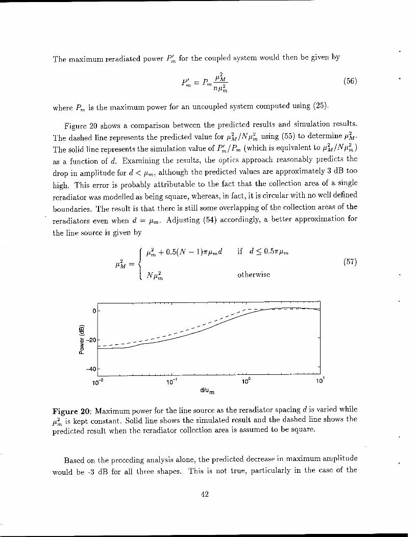
The maximum reradiated power P'm for the coupled system would then be given by

P' — P PM m o (56)

where Pm is the maximum power for an uncoupled system computed using (25).

Figure 20 shows a comparison between the predicted results and simulation results.

The dashed line represents the predicted value for n2M/Np2

m using (55) to determine fi2M.

The solid line represents the simulation value of P^/Pm (which is equivalent to PM/N^)

as a function of d. Examining the results, the optics approach reasonably predicts the

drop in amplitude for d < /zm, although the predicted values are approximately 3 dB too

high. This error is probably attributable to the fact that the collection area of a single

reradiator was modelled as being square, whereas, in fact, it is circular with no well defined

boundaries. The result is that there is still some overlapping of the collection areas of the

reradiators even when d = (im. Adjusting (54) accordingly, a better approximation for

the line source is given by

( ..2

2 PM

H2m + 0.5(N - l)TTnmd if d<0.5irnr.

(Niil

(57)

otherwise

m

0)

o Q.

-40

Figure 20: Maximum power for the line source as the reradiator spacing d is varied while H2

m is kept constant. Solid line shows the simulated result and the dashed line shows the predicted result when the reradiator collection area is assumed to be square.

Based on the preceding analysis alone, the predicted decrease in maximum amplitude

would be -3 dB for all three shapes. This is not true, particularly in the case of the

42

dumbbell. Returning to the example of the kth reradiator, two other factors which reduces

the incident signal are the number of other surrounding reradiators and the location of

these other reradiators. The decrease in incident signal as the number of surrounding

reradiators increases needs no explanation. Location plays a role in terms of distance from

the kth reradiator as well as orientation with respect to the line joining the transmitter

and kth reradiator. For example, a second reradiator lying anywhere along this line but

between the transmitter and the kth reradiator will produce a signal which is out-of-

phase with the direct signal. On the opposite side of the reradiator, away from the

transmitter (but still on the line), the signal phases from the individual reradiators will

quickly change in phase as a function of distance from the kth reradiator. This can be

summarized mathematically as,

iki

0 same side as transmitter

(58)

opposite side 47rrw

A

where r*/ is the distance between the kth and mth reradiators, and 0« is the change in

phase due to this distance. Taking path attenuations into account, it follows that the inci-

dent signal on the kth reradiator will be affected by all the reradiators between it and the

transmitter but only the reradiators out to a distance of A/4 in the opposite direction (be-

yond this distance the alternating phase greatly diminishes the contribution of reradiated

signals). Extending this analysis to all possible locations for the mth reradiator results in

regions as illustrated in Figure 21 where the white regions corresponds to 6M < "" and the

dark regions to 9^ > ir (where it is assumed 0« is normalized to the range 0 < 6ki < 2TT).

The central white region, which encompasses the transmitter and kth reradiator, is called

the first Fresnel zone [8]. The surrounding black is the second Fresnel zone, the next white

region is the third Fresnel zone, and so on. Reradiators located in the first Fresnel zone

will have the most effect on the incident signal of the kth reradiator given the size of this

zone and its proximity to the transmitter and kth reradiator. Within this region, path

losses will favour reradiators that are closer to either the transmitter or the kth reradiator.

This "shadowing" effect is important since the net result is that the row of reradiators

closest to the transmitter will be the least affected (highest incident signal) and will

therefore reradiate the highest signal. Each successive row will reradiate less and less

as more and more reradiators move into the first Fresnel zone. Comparing the three

different shapes used to produce Figures 18 and 19, the Fresnel zone effect will play the

strongest role for the dumbbell and the weakest for the line source. This is reflected in

43

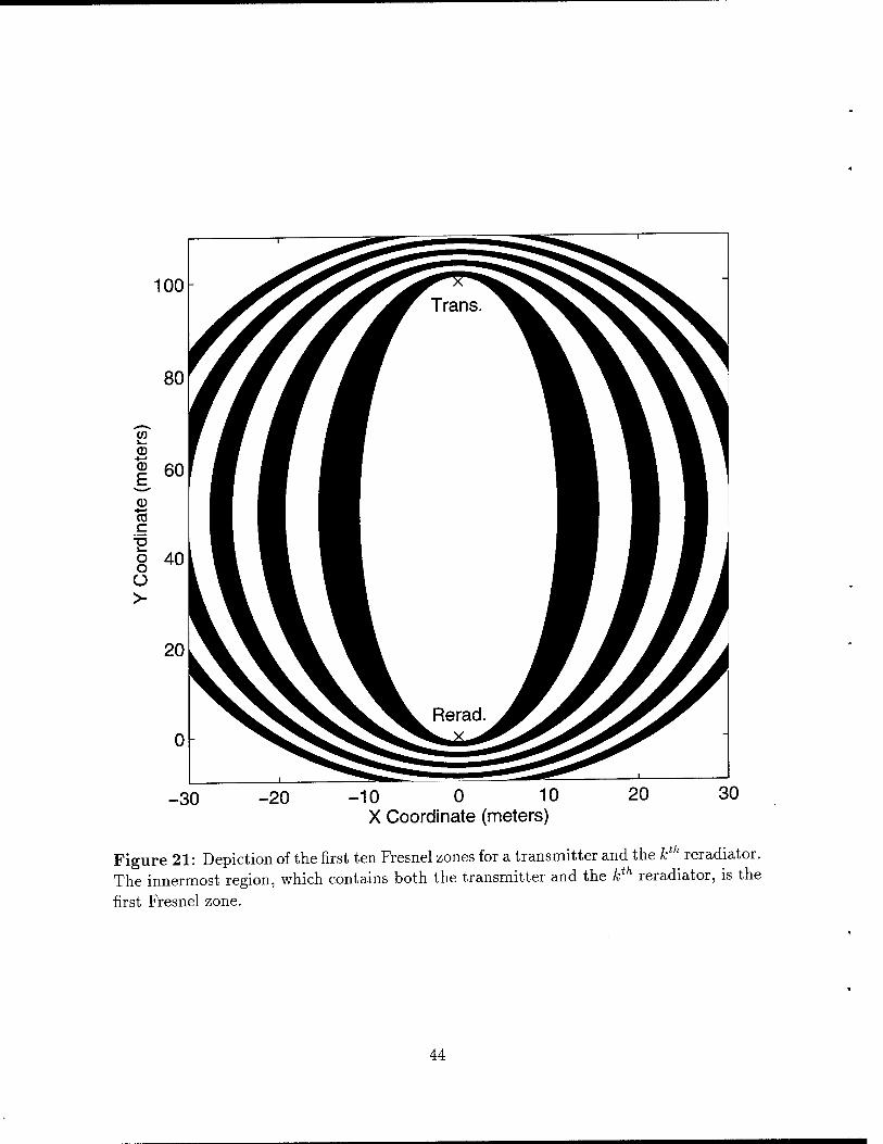
100

© -I—' o E, CD •*—' CO c

TJ L_

O o Ü

-30 -20 -10 0 10 X Coordinate (meters)

20

Figure 21: Depiction of the first ten Fresnel zones for a transmitter and the kth reradiator. The innermost region, which contains both the transmitter and the kth reradiator, is the

first Fresnel zone.

44

the amplitude differences which were -7.5 dB, -3.9 dB, and -3.2 dB for the dumbbell, the

bent cross, and the line shapes, respectively.

3.2.2 Effect on Beamwidth

Despite the changes in power and phase, and some filling in of the nulls, the shape

of the main beam remains relatively unaffected. As a result, the characterization of

beamwidth discussed in Section 2.3.2 remains valid.

3.2.3 Effect on Phase

The main affect on phase observed in Figure 19 is a constant offset of 20°-30°, and a

more gentle roll-off near the label nulls. The offset is due to the effect of the reradiators

contributing to the incident signal. For example, the incident signal for the kth reradiator

is the transmitter signal plus the contribution of the surrounding reradiators. Since the

reradiator signals will tend to involve extra path lengths compared to the transmitter

signal, the resultant incident signal will tend to be phase shifted slightly. For example,

consider one of the central reradiators in the line source, the kth reradiator. Given that

the greatest coupling is between its nearest neighbours (the (k — l)th and the (k + l)th

reradiators), then for the sake of this discussion, all other reradiators can be ignored.

Based on this simplification and using (47) the reradiated signal from the kth reradiator

is given by,

Smk = ßk{Stxpam{rak) + Smk-lpam{rkk-l) + Smk+lPam(rkk+l)) (59)

Given the translational symmetry of the line source, except near the ends, then smk-i ~

Smk ~ -Smfc+i- Using this approximation and the fact that r^k-i = Hcfc-i = Um, the above

expression can be simplified to

S-mk = Pk \StxPamy ak) T" £SmkPam\Pm))

= ßk (sixPam(rak) + S-?±e-^A (60)

45

Rearranging to solve for smk yields

_ PkstxPam\rak) (gi\ smk — a, _,-2TT„ V '

Letting s^fc represent the value when coupling is ignored where

S'mk = ßkStxpam(rak) (62)

then Smk -*-

*'«* 1-^

(63)

For a value of ßk = -1 and [im = A/10 the above formula predicts a value of smk/s'mk =

0.653 + jO.149, or a phase difference between the coupled and uncoupled cases of 12.8°.

Although somewhat smaller than the value of 26.9° shown for the line source in Figure

18a (attributable to the fact that coupling effects were restricted to the two nearest

neighbours) it does demonstrate the mechanism by which the phase offset arises.

3.2.4 Enhancement of Reflections

In Section 2.3.4, it was shown that the thickness of the multipath source (i.e. the

extent of the multipath source measured in the same direction as the transmitter signal)

had a strong effect on the power of the reflection beam, with thin sources having a stronger

reflection than thick sources. When coupling is taken into account, the reradiators on the

surface or edge closest to the transmitter receive the greatest illumination while reradiators

in successive rows behind receive less and less illumination due to shadowing effects. The

result is the reflection beam generated by the first row is not completely cancelled by the

reflections from successive rows, because successive reflections become weaker and weaker

(especially compared to the uncoupled case).

Figure 22 illustrates this phenomena showing the same results as in Figure 17 except

including coupling effects. The dashed lines represent the original results from Figure 17

which have been included for comparison. The effect of coupling on the reflection beam is

most obvious in Figure 22c where the reflection beam has been reduced but not eliminated

as happened in the uncoupled case.

46

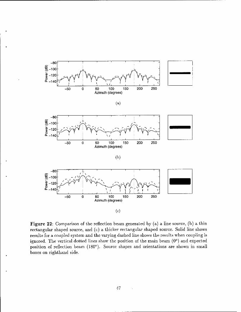
|-120 o O--140

-50 50 100 150 Azimuth (degrees)

200 250

(a)

50 100 150 Azimuth (degrees)

(b)

-80 Cß 2.-100

|-120 o Q--140

: r— i i i i

- t^ir ■\0 - -

V^ o/T\ -

. Yil'f i' i ' \" J t J i V

-50 0 50 100 150 200 250 Azimuth (degrees)

(c)

Figure 22: Comparison of the reflection beam generated by (a) a line source, (b) a thin rectangular shaped source, and (c) a thicker rectangular shaped source. Solid line shows results for a coupled system and the varying dashed line shows the results when coupling is ignored. The vertical dotted lines show the position of the main beam (0°) and expected position of reflection beam (180°). Source shapes and orientations are shown in small boxes on righthand side.

47

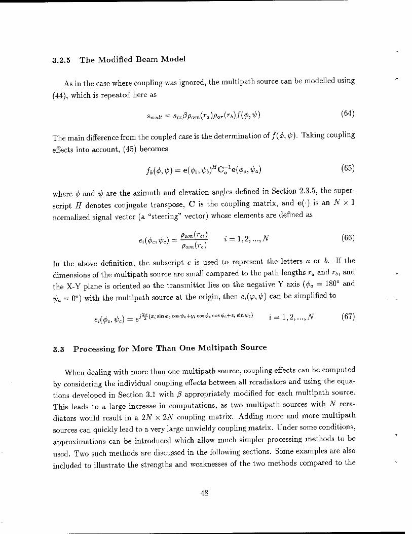
3.2.5 The Modified Beam Model

As in the case where coupling was ignored, the multipath source can be modelled using

(44), which is repeated here as

Smult = Stxßpam{ra)par{n)f(<i>^) (64)

The main difference from the coupled case is the determination of f(<j>, ip). Taking coupling

effects into account, (45) becomes

fk(<j>^) = e(<t>b,i>b)HC-1e(<j>a,4>a) (65)

where (f> and ^ are the azimuth and elevation angles defined in Section 2.3.5, the super-

script H denotes conjugate transpose, C is the coupling matrix, and e(-) is an N x 1

normalized signal vector (a "steering" vector) whose elements are defined as

e^M = P-^\ i = l,2,...,N (66)

In the above definition, the subscript c is used to represent the letters a or b. If the

dimensions of the multipath source are small compared to the path lengths ra and rb, and

the X-Y plane is oriented so the transmitter lies on the negative Y axis ((j)a = 180° and

ij}a = 0°) with the multipath source at the origin, then e,-(<p,^) can be simplified to

IX JjJ _ ei^(a;, sin0c cos Vc+yi cos0c cos Vc+^i sin Vc) i = l,2, ...,N (67)

3.3 Processing for More Than One Multipath Source

When dealing with more than one multipath source, coupling effects can be computed

by considering the individual coupling effects between all reradiators and using the equa-

tions developed in Section 3.1 with ß appropriately modified for each multipath source.

This leads to a large increase in computations, as two multipath sources with N rera-

diators would result in a 2N x 2iV coupling matrix. Adding more and more multipath

sources can quickly lead to a very large unwieldy coupling matrix. Under some conditions,

approximations can be introduced which allow much simpler processing methods to be

used. Two such methods are discussed in the following sections. Some examples are also

included to illustrate the strengths and weaknesses of the two methods compared to the

48

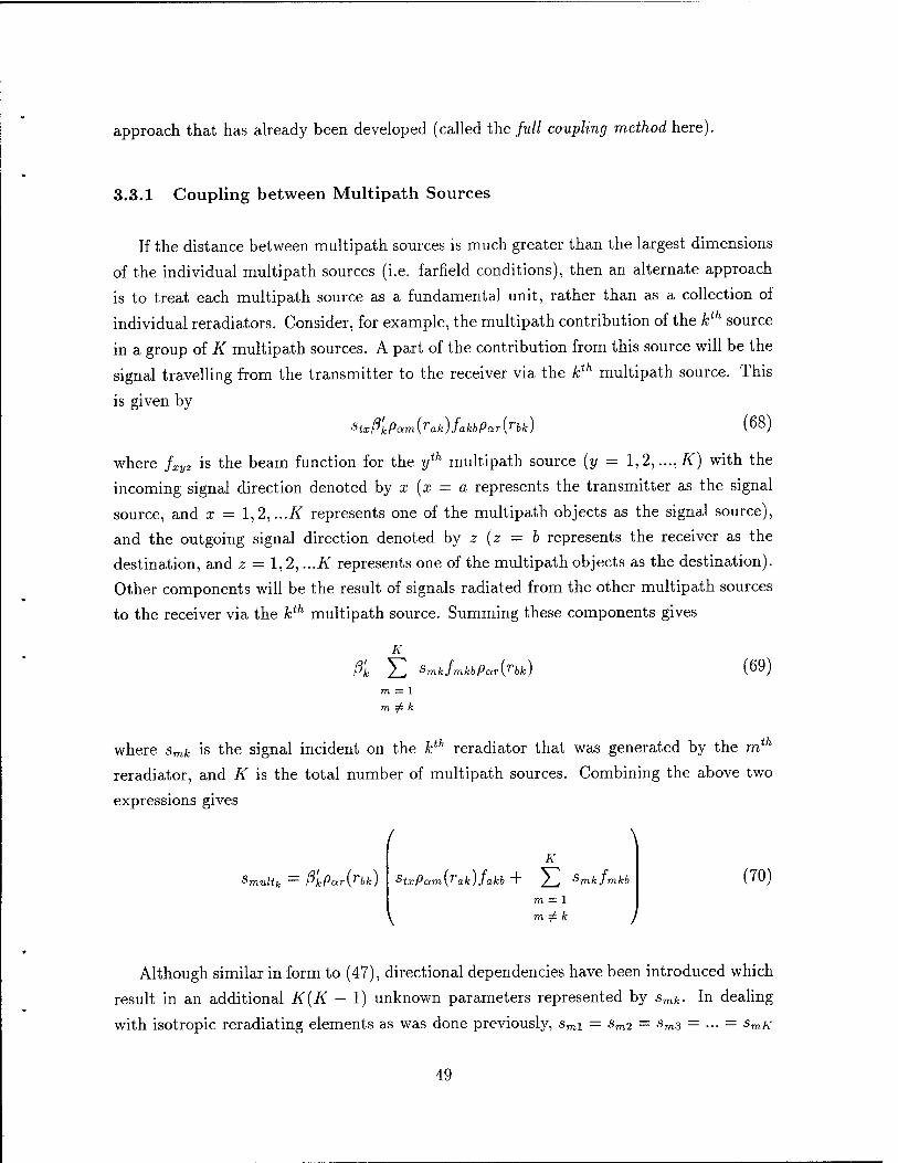
approach that has already been developed (called the full coupling method here).

3.3.1 Coupling between Multipath Sources

If the distance between multipath sources is much greater than the largest dimensions

of the individual multipath sources (i.e. farfield conditions), then an alternate approach

is to treat each multipath source as a fundamental unit, rather than as a collection of

individual reradiators. Consider, for example, the multipath contribution of the kth source

in a group of K multipath sources. A part of the contribution from this source will be the

signal travelling from the transmitter to the receiver via the kth multipath source. This

is given by

Stxß'kPam(rak)fakbpar(rbk) (68)

where fxyz is the beam function for the yth multipath source (y = 1,2,..., K) with the

incoming signal direction denoted by x (x = a represents the transmitter as the signal

source, and x = 1,2,...K represents one of the multipath objects as the signal source),

and the outgoing signal direction denoted by z (z = b represents the receiver as the

destination, and z — 1,2,...K represents one of the multipath objects as the destination).

Other components will be the result of signals radiated from the other multipath sources

to the receiver via the kth multipath source. Summing these components gives

K

ß'k H SmkfmkbPar{rbk) (69) m = 1

m ^ k

where smk is the signal incident on the kth reradiator that was generated by the mth

reradiator, and K is the total number of multipath sources. Combining the above two

expressions gives

Smultk — PkPar\rbk)

( \

K

StxPamyakjJakb ~r / , Smkjmkb

m = 1 y m# k )

(70)

Although similar in form to (47), directional dependencies have been introduced which

result in an additional K(K - 1) unknown parameters represented by smk- In dealing

with isotropic reradiating elements as was done previously, sml = sm2 = sm3 = ... = smK

49

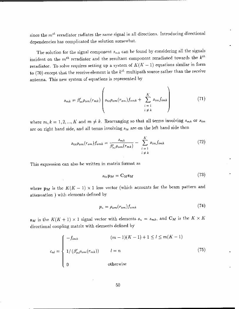
since the mth reradiator radiates the same signal in all directions. Introducing directional

dependencies has complicated the solution somewhat.

The solution for the signal component smk can be found by considering all the signals

incident on the mth reradiator and the resultant component reradiated towards the kth

reradiator. To solve requires setting up a system of K(K - 1) equations similar in form

to (70) except that the receive element is the kth multipath source rather than the receive

antenna. This new system of equations is represented by

/

smk — PmPam\Tmk)

\ K

Stxpam[ram)jamk "r /_^ simjimk

i = 1 i±k I

(71)

where m, k = 1,2,...,K and m / k. Rearranging so that all terms involving smk or st-.

on right hand side, and all terms involving stx are on the left hand side then are

StxPamyamJJamk Smk

PmPam{rmk, / j Simjh (72)

% = l

i^k

This expression can also be written in matrix format as

StxPM — CA/SM (73)

where pM is the K(K - 1) x 1 loss vector (which accounts for the beam pattern and

attenuation ) with elements defined by

Pn — pamyamjjamk (74)

SM is the K(K + 1) x 1 signal vector with elements sn = smk, and CM is the K x K

directional coupling matrix with elements defined by

Cnl =

-/.■■ rak (m - 1)(K -!) + !</< m(K - 1)

lliß'mPcxmirmk)) I — n

otherwise

(75)

50

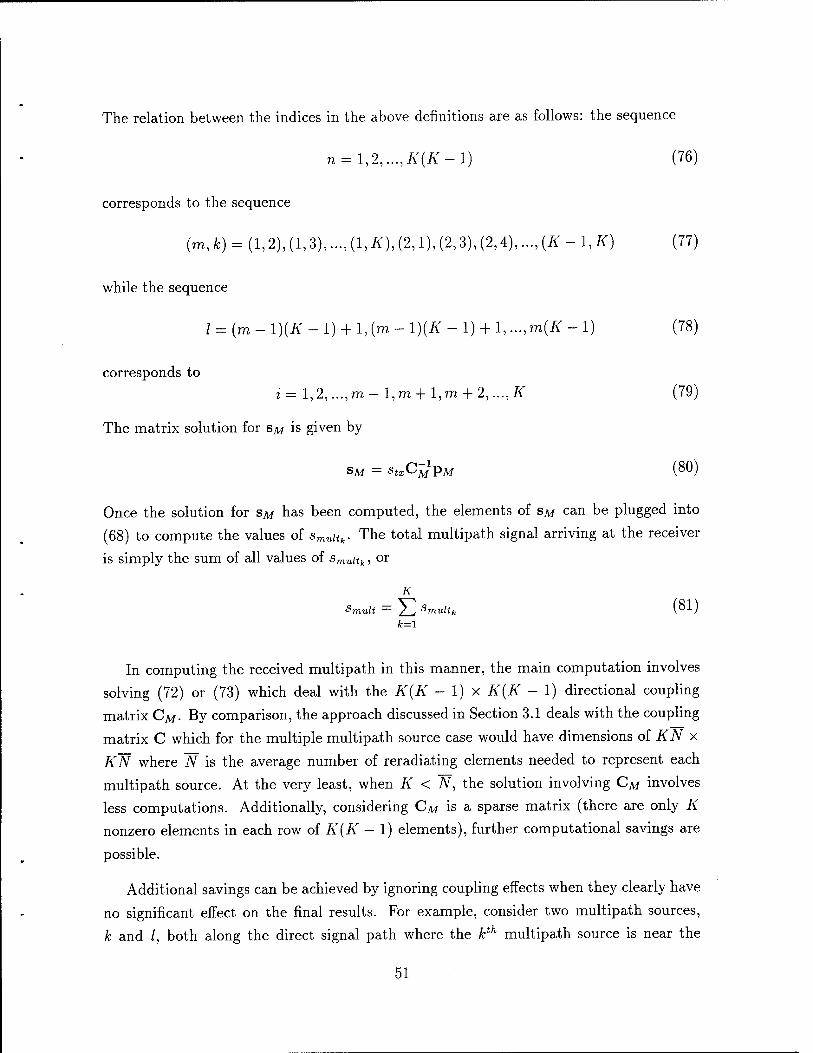
The relation between the indices in the above definitions are as follows: the sequence

n = l,2,...,K(K-l) (76)

corresponds to the sequence

(m,fc) = (l,2),(l,3),...,(l,/0,(2,l),(2,3),(2,4),...,(A'-l,/0 (77)

while the sequence

/ = (m - 1)(K - 1) + 1, (m - \){K - 1) + 1,..., m(K - 1) (78)

corresponds to

t = l,2,...,m-l,ro+l,m + 2,...,Är (79)

The matrix solution for SM is given by

% = stxC^pM (80)

Once the solution for sM has been computed, the elements of sM can be plugged into

(68) to compute the values of smuHk. The total multipath signal arriving at the receiver

is simply the sum of all values of smuuk, or

K

Smult = z2 Smultk (81) fc=l

In computing the received multipath in this manner, the main computation involves

solving (72) or (73) which deal with the K(K - 1) x K(K - 1) directional coupling

matrix CM- By comparison, the approach discussed in Section 3.1 deals with the coupling

matrix C which for the multiple multipath source case would have dimensions of KN x

KN where ~N is the average number of reradiating elements needed to represent each

multipath source. At the very least, when K < N, the solution involving CM involves

less computations. Additionally, considering CM is a sparse matrix (there are only K

nonzero elements in each row of K(K — 1) elements), further computational savings are

possible.

Additional savings can be achieved by ignoring coupling effects when they clearly have

no significant effect on the final results. For example, consider two multipath sources,

k and /, both along the direct signal path where the kth multipath source is near the

51

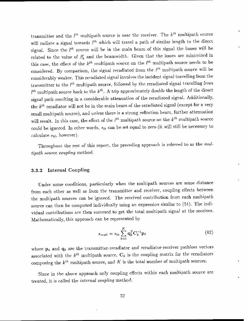
transmitter and the Ith multipath source is near the receiver. The kth multipath source

will radiate a signal towards Ith which will travel a path of similar length to the direct

signal. Since the Ith source will be in the main beam of this signal the losses will be

related to the value of ß'k and the beamwidth. Given that the losses are minimized in

this case, the effect of the kth multipath source on the Ith multipath source needs to be

considered. By comparison, the signal reradiated from the Ith multipath source will be

considerably weaker. This reradiated signal involves the incident signal travelling from the

transmitter to the Ith multipath source, followed by the reradiated signal travelling from

Ith multipath source back to the kth. A trip approximately double the length of the direct

signal path resulting in a considerable attenuation of the reradiated signal. Additionally,

the kth reradiator will not be in the main beam of the reradiated signal (except for a very

small multipath source), and unless there is a strong reflection beam, further attenuation

will result. In this case, the effect of the Ith multipath source on the kth multipath source

could be ignored. In other words, slk can be set equal to zero (it will still be necessary to

calculate ski, however).

Throughout the rest of this report, the preceding approach is referred to as the mul-

tipath source coupling method.

3.3.2 Internal Coupling

Under some conditions, particularly when the multipath sources are some distance

from each other as well as from the transmitter and receiver, coupling effects between

the multipath sources can be ignored. The received contribution from each multipath

source can then be computed individually using an expression similar to (54). The indi-

vidual contributions are then summed to get the total multipath signal at the receiver.

Mathematically, this approach can be represented by

K

I Smult = Stx YJ vlC^Pk (82)

where pk and qk are the transmitter-reradiator and reradiator-receiver pathloss vectors

associated with the kth multipath source, Ck is the coupling matrix for the reradiators

composing the kth multipath source, and K is the total number of multipath sources.

Since in the above approach only coupling effects within each multipath source are

treated, it is called the internal coupling method.

52

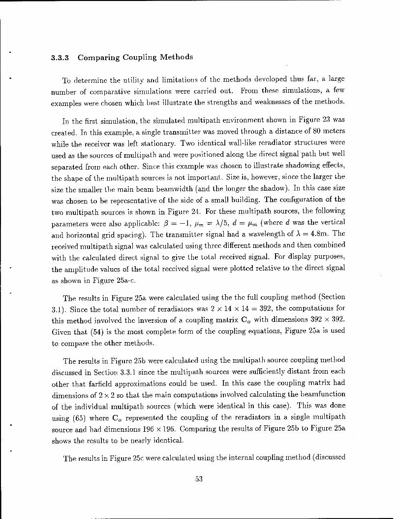
3.3.3 Comparing Coupling Methods

To determine the utility and limitations of the methods developed thus far, a large

number of comparative simulations were carried out. From these simulations, a few

examples were chosen which best illustrate the strengths and weaknesses of the methods.

In the first simulation, the simulated multipath environment shown in Figure 23 was

created. In this example, a single transmitter was moved through a distance of 80 meters

while the receiver was left stationary. Two identical wall-like reradiator structures were

used as the sources of multipath and were positioned along the direct signal path but well

separated from each other. Since this example was chosen to illustrate shadowing effects,

the shape of the multipath sources is not important. Size is, however, since the larger the

size the smaller the main beam beamwidth (and the longer the shadow). In this case size

was chosen to be representative of the side of a small building. The configuration of the

two multipath sources is shown in Figure 24. For these multipath sources, the following

parameters were also applicable: ß = -1, \xm = A/5, d = \im (where d was the vertical

and horizontal grid spacing). The transmitter signal had a wavelength of A = 4.8m. The

received multipath signal was calculated using three different methods and then combined

with the calculated direct signal to give the total received signal. For display purposes,

the amplitude values of the total received signal were plotted relative to the direct signal

as shown in Figure 25a-c.

The results in Figure 25a were calculated using the the full coupling method (Section

3.1). Since the total number of reradiators was 2 x 14 x 14 = 392, the computations for

this method involved the inversion of a coupling matrix Ca with dimensions 392 x 392.

Given that (54) is the most complete form of the coupling equations, Figure 25a is used

to compare the other methods.

The results in Figure 25b were calculated using the multipath source coupling method

discussed in Section 3.3.1 since the multipath sources were sufficiently distant from each

other that farfield approximations could be used. In this case the coupling matrix had

dimensions of 2 x 2 so that the main computations involved calculating the beamfunction

of the individual multipath sources (which were identical in this case). This was done

using (65) where Ca represented the coupling of the reradiators in a single multipath

source and had dimensions 196 x 196. Comparing the results of Figure 25b to Figure 25a

shows the results to be nearly identical.

The results in Figure 25c were calculated using the internal coupling method (discussed

53

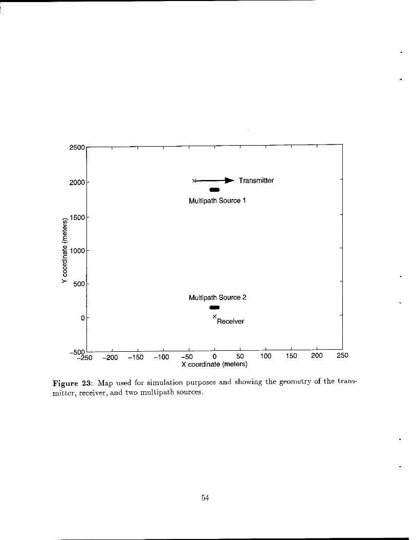
2500

2000

.-.1500 0) i— (D

■t—'

E,

|j 1000 c

O O Ü

>- 500

-500

Transmitter

Multipath Source 1

Multipath Source 2

x Receiver

250 -200 -150 -100 -50 0 50 100 150 200 250 X coordinate (meters)

Figure 23: Map used for simulation purposes and showing the geometry of the trans- mitter, receiver, and two multipath sources.

54

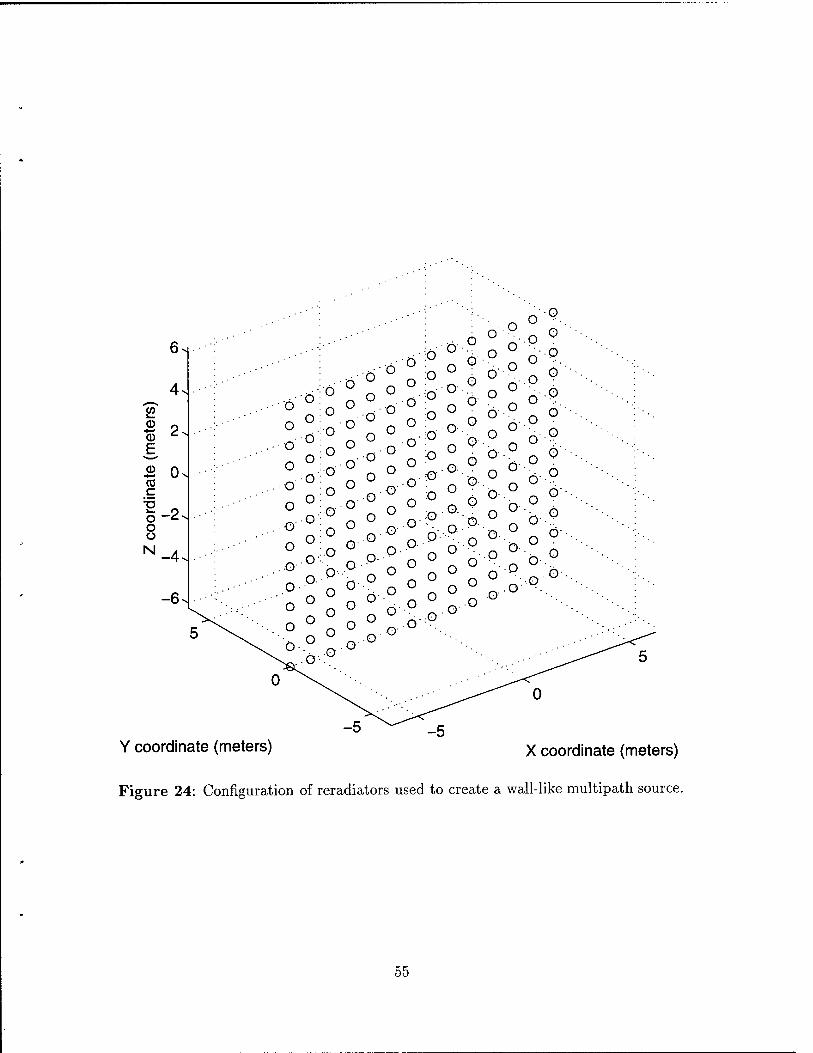
61

4. fft 1_

o 0 2v

E ^■^

0 Os CO c

T5 O -2 s o Ü

N -4v

-6v

o o o o o o

.©■

o . o .0 o

Ö

o ■o

o •Ö

o o o o p o p o

o p p' o o o o o o p o o o

p o o' o o o o o o p o o p

o p p p- p p p p-

p 'p. p o o

■ O

o o p' o b o p o p- o Ö-

p o

■O

p o'

o .o

6°. o ° A o

o p ° o

p- p

.o

o p

•O'

Q p

■ P

p

• P o .0 6'

p' p p- p

Y coordinate (meters) X coordinate (meters)

Figure 24: Configuration of reradiators used to create a wall-like multipath source.

55

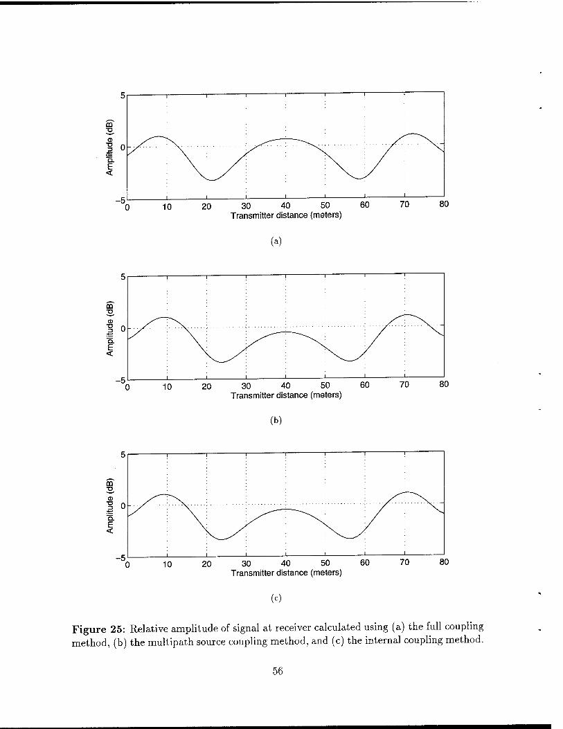
10 20 30 40 50 Transmitter distance (meters)

60 70 80

;o

T3

Q. E <

-5

1 —i 1 1 ! i !

10 20 30 40 50 Transmitter distance (meters)

60 70 80

(b)

10 20 30 40 50 Transmitter distance (meters)

60 70 80

(c)

Figure 25: Relative amplitude of signal at receiver calculated using (a) the full coupling method, (b) the multipath source coupling method, and (c) the internal coupling method.

56

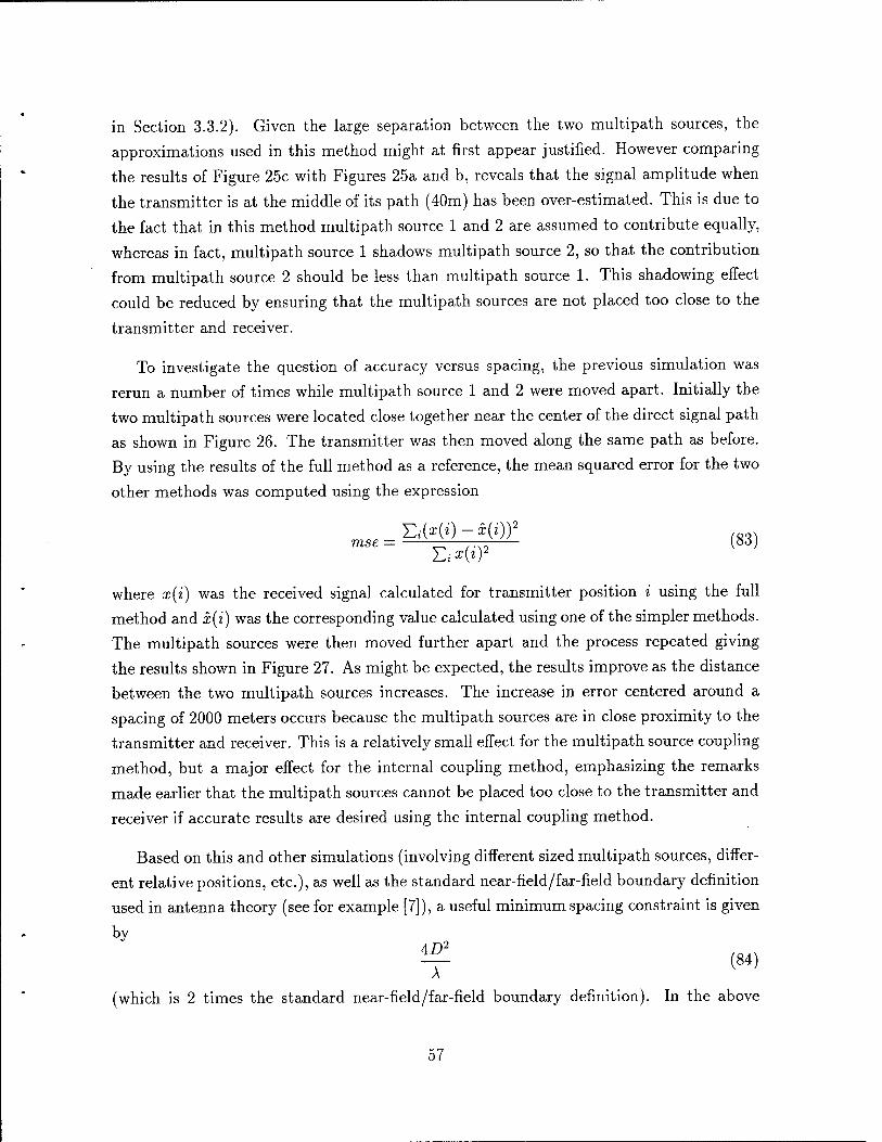
in Section 3.3.2). Given the large separation between the two multipath sources, the

approximations used in this method might at first appear justified. However comparing

the results of Figure 25c with Figures 25a and b, reveals that the signal amplitude when

the transmitter is at the middle of its path (40m) has been over-estimated. This is due to

the fact that in this method multipath source 1 and 2 are assumed to contribute equally,

whereas in fact, multipath source 1 shadows multipath source 2, so that the contribution

from multipath source 2 should be less than multipath source 1. This shadowing effect

could be reduced by ensuring that the multipath sources are not placed too close to the

transmitter and receiver.

To investigate the question of accuracy versus spacing, the previous simulation was

rerun a number of times while multipath source 1 and 2 were moved apart. Initially the

two multipath sources were located close together near the center of the direct signal path

as shown in Figure 26. The transmitter was then moved along the same path as before.

By using the results of the full method as a reference, the mean squared error for the two

other methods was computed using the expression

mse= E,*W (83)

where x(i) was the received signal calculated for transmitter position i using the full

method and x(i) was the corresponding value calculated using one of the simpler methods.

The multipath sources were then moved further apart and the process repeated giving

the results shown in Figure 27. As might be expected, the results improve as the distance

between the two multipath sources increases. The increase in error centered around a

spacing of 2000 meters occurs because the multipath sources are in close proximity to the

transmitter and receiver. This is a relatively small effect for the multipath source coupling

method, but a major effect for the internal coupling method, emphasizing the remarks

made earlier that the multipath sources cannot be placed too close to the transmitter and

receiver if accurate results are desired using the internal coupling method.

Based on this and other simulations (involving different sized multipath sources, differ-

ent relative positions, etc.), as well as the standard near-field/far-field boundary definition

used in antenna theory (see for example [7]), a useful minimum spacing constraint is given

AD2

-T (84)

(which is 2 times the standard near-field/far-field boundary definition). In the above

57

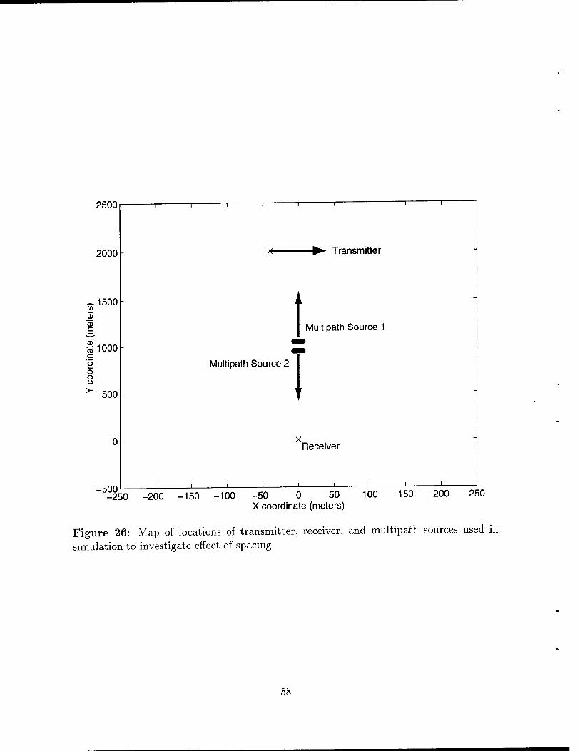
2500

2000

^1500 w k_

B o5

% 1000 c

O o Ü

500

-500

-i r

>f> Transmitter

Multipath Source 1

Multipath Source 2

x Receiver

J L. J l_ J 1_

-250 -200 -150 -100 -50 0 50 100 150 200 250 X coordinate (meters)

Figure 26: Map of locations of transmitter, receiver, and multipath sources used in simulation to investigate effect of spacing.

58

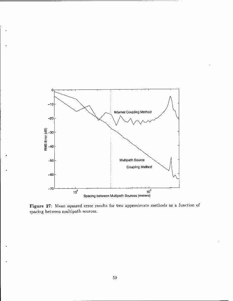
-10

-20

2.-30

-40

-50

-60

-70

Multipath Source

Coupling Method

10Z 10° Spacing between Multipath Sources (meters)

Figure 27: Mean squared error results for two approximate methods as a function of

spacing between multipath sources.

59

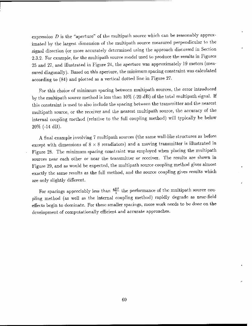
expression D is the "aperture" of the multipath source which can be reasonably approx-

imated by the largest dimension of the multipath source measured perpendicular to the

signal direction (or more accurately determined using the approach discussed in Section

2.3.2. For example, for the multipath source model used to produce the results in Figures

25 and 27, and illustrated in Figure 24, the aperture was approximately 19 meters (mea-

sured diagonally). Based on this aperture, the minimum spacing constraint was calculated

according to (84) and plotted as a vertical dotted line in Figure 27.

For this choice of minimum spacing between multipath sources, the error introduced

by the multipath source method is less than 10% (-20 dB) of the total multipath signal. If

this constraint is used to also include the spacing between the transmitter and the nearest

multipath source, or the receiver and the nearest multipath source, the accuracy of the

internal coupling method (relative to the full coupling method) will typically be below

20% (-14 dB).

A final example involving 7 multipath sources (the same wall-like structures as before

except with dimensions of 8 x 8 reradiators) and a moving transmitter is illustrated in

Figure 28. The minimum spacing constraint was employed when placing the multipath

sources near each other or near the transmitter or receiver. The results are shown in

Figure 29, and as would be expected, the multipath source coupling method gives almost

exactly the same results as the full method, and the source coupling gives results which

are only slightly different.

For spacings appreciably less than ^ the performance of the multipath source cou-

pling method (as well as the internal coupling method) rapidly degrade as near-field

effects begin to dominate. For these smaller spacings, more work needs to be done on the

development of computationally efficient and accurate approaches.

60

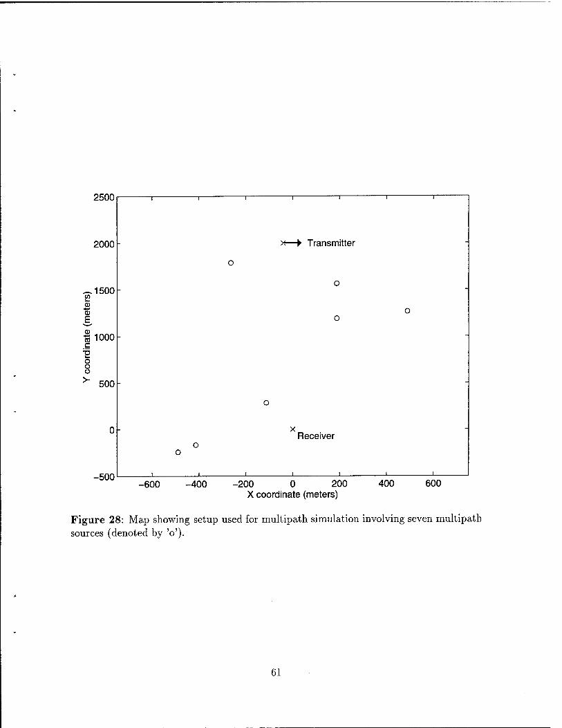
2500

2000

^1500 52 CD *-» CD

■§ 1000 c

o o o 500

-500

-

I I I

o

1 1

><—► Transmitter

i i

- o

o

-

o

-

-

o

-

o o

I 1

X Receiver

i i i i

-600 -400 -200 0 200 X coordinate (meters)

400 600

Figure 28: Map showing setup used for multipath simulation involving seven multipath sources (denoted by V).

61

10 20 30 40 50 Transmitter distance (meters)

60 70 80

(a)

10 20 30 40 50 Transmitter distance (meters)

60 70 80

(b)

S °-5

3 Or Q. E <-0.5

-1 10 20 30 40 50

Transmitter distance (meters) 60 70 80

(c)

Figure 29: Multipath simulation showing relative amplitude of signal at the receiver calculated using (a) the full coupling method, (b) the multipath source coupling method,

and (c) the internal coupling method.

62

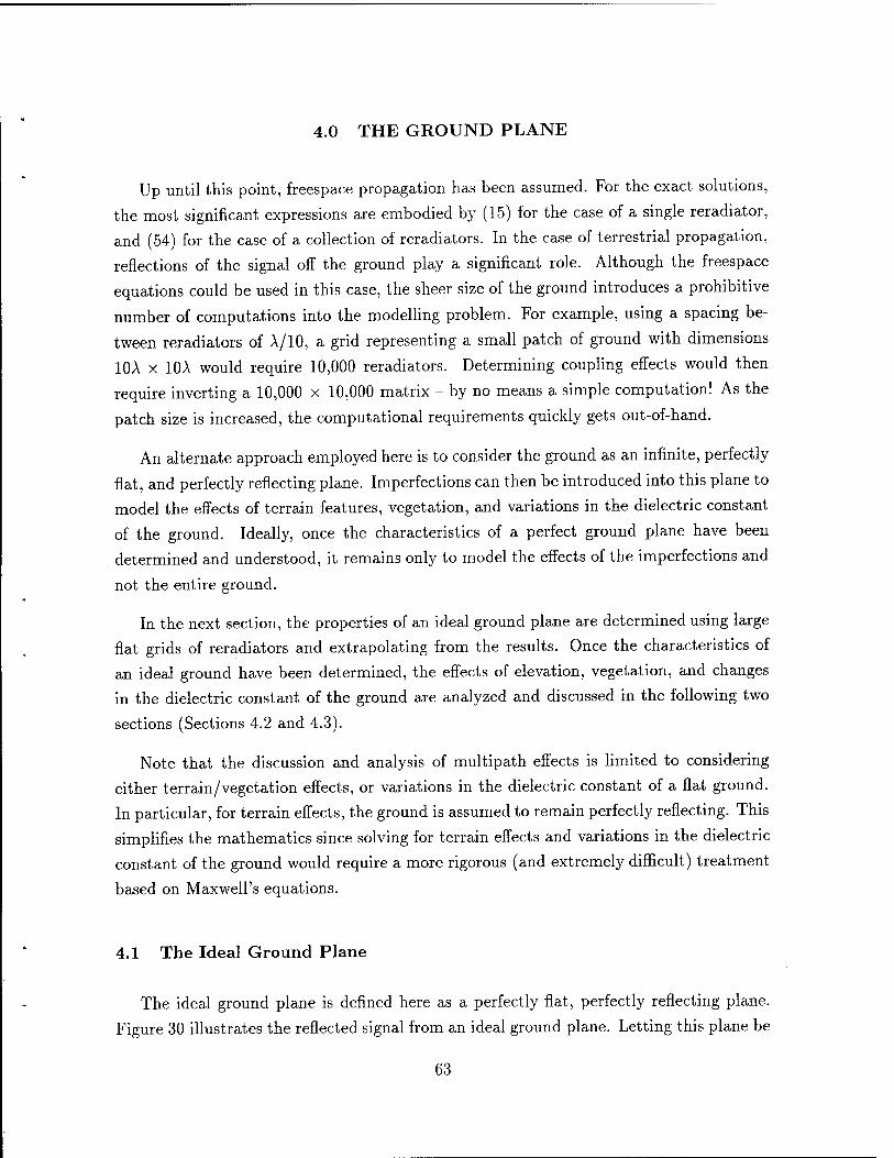
4.0 THE GROUND PLANE

Up until this point, freespace propagation has been assumed. For the exact solutions,

the most significant expressions are embodied by (15) for the case of a single reradiator,

and (54) for the case of a collection of reradiators. In the case of terrestrial propagation,

reflections of the signal off the ground play a significant role. Although the freespace

equations could be used in this case, the sheer size of the ground introduces a prohibitive

number of computations into the modelling problem. For example, using a spacing be-

tween reradiators of A/10, a grid representing a small patch of ground with dimensions

10A x 10A would require 10,000 reradiators. Determining coupling effects would then

require inverting a 10,000 x 10,000 matrix - by no means a simple computation! As the

patch size is increased, the computational requirements quickly gets out-of-hand.

An alternate approach employed here is to consider the ground as an infinite, perfectly

flat, and perfectly reflecting plane. Imperfections can then be introduced into this plane to

model the effects of terrain features, vegetation, and variations in the dielectric constant

of the ground. Ideally, once the characteristics of a perfect ground plane have been

determined and understood, it remains only to model the effects of the imperfections and

not the entire ground.

In the next section, the properties of an ideal ground plane are determined using large

flat grids of reradiators and extrapolating from the results. Once the characteristics of

an ideal ground have been determined, the effects of elevation, vegetation, and changes

in the dielectric constant of the ground are analyzed and discussed in the following two

sections (Sections 4.2 and 4.3).

Note that the discussion and analysis of multipath effects is limited to considering

either terrain/vegetation effects, or variations in the dielectric constant of a flat ground.

In particular, for terrain effects, the ground is assumed to remain perfectly reflecting. This

simplifies the mathematics since solving for terrain effects and variations in the dielectric

constant of the ground would require a more rigorous (and extremely difficult) treatment

based on Maxwell's equations.

4.1 The Ideal Ground Plane

The ideal ground plane is defined here as a perfectly flat, perfectly reflecting plane.

Figure 30 illustrates the reflected signal from an ideal ground plane. Letting this plane be

63

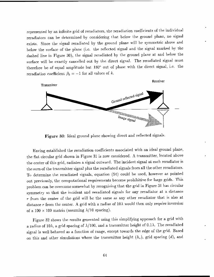
represented by an infinite grid of reradiators, the reradiation coefficients of the individual

reradiators can be determined by considering that below the ground plane, no signal

exists. Since the signal reradiated by the ground plane will be symmetric above and

below the surface of the plane (i.e. the reflected signal and the signal marked by the

dashed line in Figure 30), the signal reradiated by the ground plane at and below the

surface will be exactly cancelled out by the direct signal. The reradiated signal must

therefore be of equal amplitude but 180° out of phase with the direct signal, i.e. the

reradiation coefficient ßk = -1 for all values of k.

Receiver Transmitter

Slgoa]

Figure 30: Ideal ground plane showing direct and reflected signals.

Having established the reradiation coefficients associated with an ideal ground plane,

the flat circular grid shown in Figure 31 is now considered. A transmitter, located above

the center of this grid, radiates a signal outward. The incident signal at each reradiator is

the sum of the transmitter signal plus the reradiated signals from all the other reradiators.

To determine the reradiated signals, equation (54) could be used, however as pointed

out previously, the computational requirements become prohibitive for large grids. This

problem can be overcome somewhat by recognizing that the grid in Figure 31 has circular

symmetry so that the incident and reradiated signals for any reradiator at a distance

r from the center of the grid will be the same as any other reradiator that is also at

distance r from the center. A grid with a radius of 10A would then only require inversion

of a 100 x 100 matrix (assuming A/10 spacing).

Figure 32 shows the results generated using this simplifying approach for a grid with

a radius of 10A, a grid spacing of A/100, and a transmitter height of 0.1A. The reradiated

signal is well behaved as a function of range, except towards the edge of the grid. Based

on this and other simulations where the transmitter height (ha), grid spacing (d), and

64

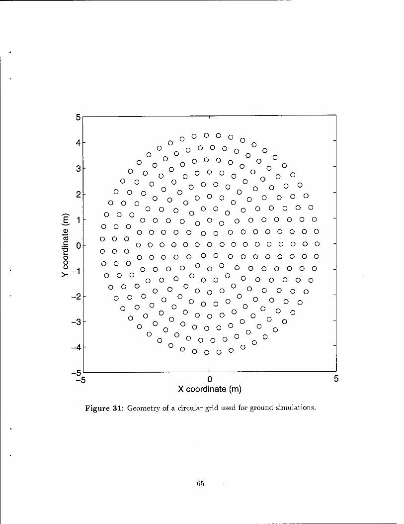
3

2

g 1 CD co

% o 1_ O O

-2

-3

-4

-5

5

o o°°on Un

Oo0°0oOo0 o°o0 ° ° o "o - 0 0 - o o - o

° ° ° O o ° o o o ° o o o o o ooo uo ou ^ _ ooo °°° o°°o oooooo

OOOO nOn oOOOOOO OOO u u

ooooo oo oooooooo ooo oooooooooooooooo ooo _ _ ooooo oo oooooooo ° oooo°o° ooooooo 000 ooo °oo° oooooo ooo ^ n o n _ o o0^o0o ooooo

o o G~ ~ o o o °0°_o o o 0000° ° O o O O °n° °° oo° o uu on^ 0o^n

wo0ow on

°o °OoooO°oo

° ° o o o o °

5 0 X coordinate (m)

Figure 31: Geometry of a circular grid used for ground simulations.

65

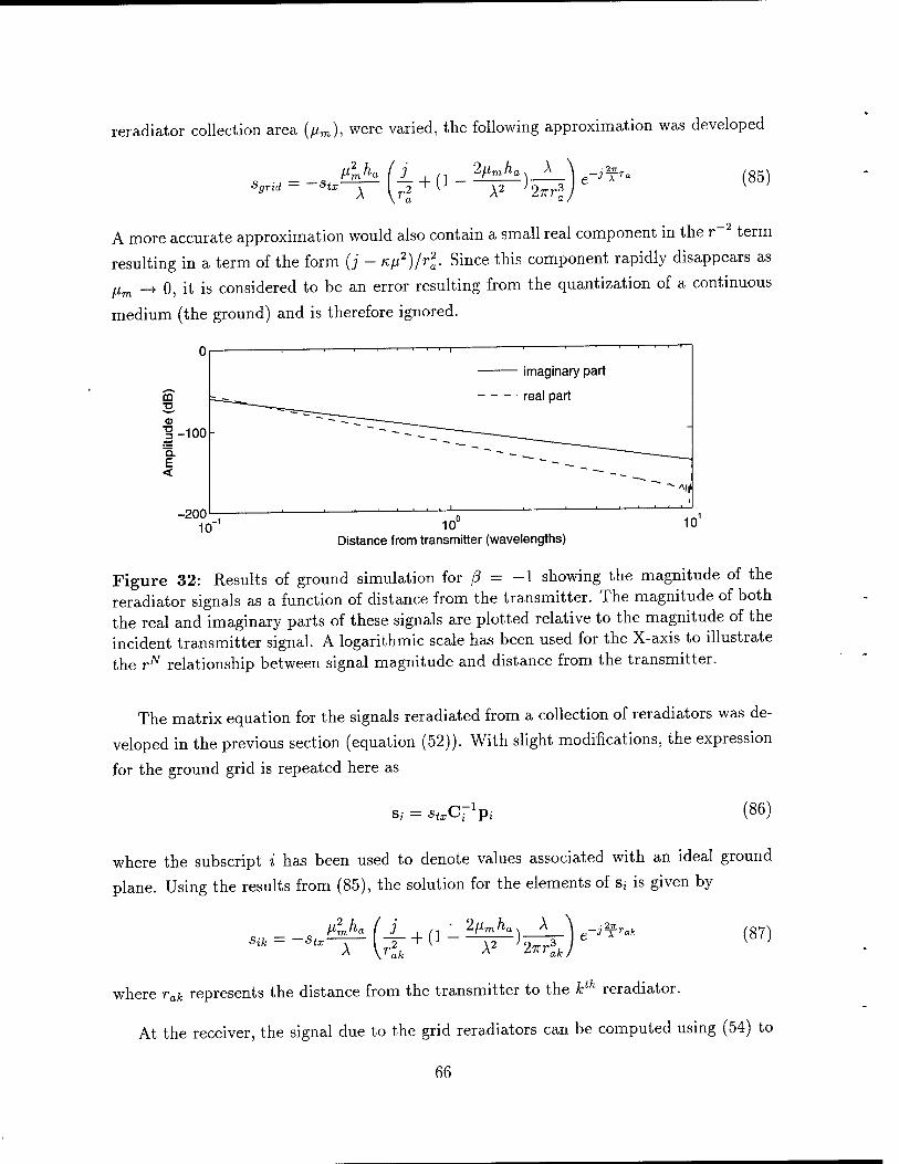
reradiator collection area (fim), were varied, the following approximation was developed

Sgrid $tx~ Vmha

A 4 + (i 2/<m^ax A •2JT„

A2 ;2;rr3 (85)

A more accurate approximation would also contain a small real component in the r~2 term

resulting in a term of the form (j - nfi2)/r2a. Since this component rapidly disappears as

fim -> 0, it is considered to be an error resulting from the quantization of a continuous

medium (the ground) and is therefore ignored.

- imaginary part

real part

Distance from transmitter (wavelengths)

Figure 32: Results of ground simulation for ß = -1 showing the magnitude of the reradiator signals as a function of distance from the transmitter. The magnitude of both the real and imaginary parts of these signals are plotted relative to the magnitude of the incident transmitter signal. A logarithmic scale has been used for the X-axis to illustrate the rN relationship between signal magnitude and distance from the transmitter.

The matrix equation for the signals reradiated from a collection of reradiators was de-

veloped in the previous section (equation (52)). With slight modifications, the expression

for the ground grid is repeated here as

Si = StxCi p (86)

where the subscript i has been used to denote values associated with an ideal ground

plane. Using the results from (85), the solution for the elements of s,- is given by

■Sj'fc ,bö(i + (i:^)r4le-*

A ak A2 '2TIT3

(87) ak ,

where rak represents the distance from the transmitter to the kth reradiator.

At the receiver, the signal due to the grid reradiators can be computed using (54) to

66

give

Sri = StxqfC^Pi (88)

Incorporating the results given in (87), and the definition for the elements of q, (53), then

the solution is given by the summation of the individual paths

Sri = -*.£ $P^ (4- + (1 - ^T^^TV) e-^(-+-fc) (89) X 2y/^Xrbk \rlk A2 27rrlJ

Alternatively, the solution for sri can also be computed by considering the fact that

since the ground grid was set up to be a perfect reflector, the resultant received signal

will be the same as a direct (unreflected) signal which travels a path of the same length

but with a 180° phase reversal (due to the reflection). This leads to,

•SH = stxpar{ri) (90)

where the path length is given by

Ti = y/(ra + rb)* + (ha + hb)* (91)

Given the derivation for the ideal ground plane grid, it is useful at this point to provide

a mathematical definition of multipath. As mentioned in the introduction, reflections

off the ground plane are an unavoidable consequence of terrestrial propagation. Hence,

multipath is defined as the difference between the actual received signal and the received

signal in the ideal case, or

Smult = ^receiver ^idea/ V^^l

Since the direct signal is the same in the ideal and nonideal cases, then multipath reduces

to the difference between the received grid signals in the two cases. Mathematically

smult — srg sri v""/

where srg is the actual signal received from the ground grid (including multipath sources).

Exploring ways to simplify the above expression, given different assumptions about the

ground, is the topic of the next section.

67

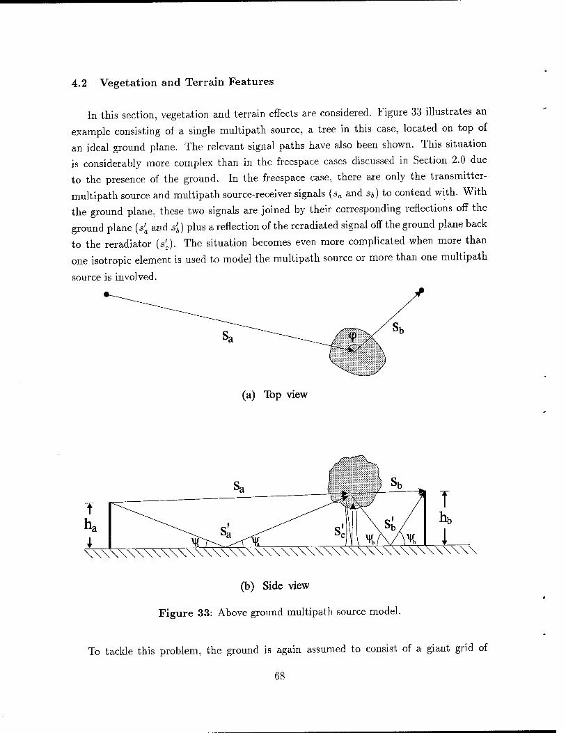
4.2 Vegetation and Terrain Features

In this section, vegetation and terrain effects are considered. Figure 33 illustrates an

example consisting of a single multipath source, a tree in this case, located on top of

an ideal ground plane. The relevant signal paths have also been shown. This situation

is considerably more complex than in the freespace cases discussed in Section 2.0 due

to the presence of the ground. In the freespace case, there are only the transmitter-

multipath source and multipath source-receiver signals (sa and sb) to contend with. With

the ground plane, these two signals are joined by their corresponding reflections off the

ground plane (s'a and s'b) plus a reflection of the reradiated signal off the ground plane back

to the reradiator (s'c). The situation becomes even more complicated when more than

one isotropic element is used to model the multipath source or more than one multipath

source is involved.

(a) Top view

(b) Side view

Figure 33: Above ground multipath source model.

To tackle this problem, the ground is again assumed to consist of a giant grid of

68

isotropic reradiators. In the absence of any multipath sources, the received signal is given

by (88) which is repeated here as,

Sri — stx<\i {->{ Pi (94)

If vegetation and/or terrain features exist on top of or above (not below) the ground plane,

then each feature can be modelled by collections of isotropic reradiators. The received

signal in this case is given by the freespace equation, namely,

Srg — stxq.aCQ Pa (95)

This expression gives very little insight into the effect of the new reradiators so that it is

useful to re-express pa, qa, and Ca, in terms of the ideal ground parameters p2, q;, and

C,. Accordingly, pa becomes

Pa

the attenuation vector q; becomes

qa

Pi

Pm

q.-

qm

(96)

(97)

and the coupling matrix C becomes

Ca C,- M

MT Cm

(98)

where M represents the coupling between the new reradiators and the ground plane, and

Cm represents the mutual coupling between the new reradiators.

The inversion of the expanded form of C can be accomplished using the matrix inver-

sion formula [9] which is repeated here as

A D

C B

A1+ A^DA^CA1 -A^DA1

-A^CA-1 A"1 (99)

69

where A = B — CA *D. Applying this formula to C then

In this expression R is given by

C"1 + C-1MR-1MTC-1 -C^MR"1

-R-VC-1 R-1 (100)

R = Cm-MTC-1M (101)

Before continuing, the expression for R deserves closer attention. The first term

obviously represents the mutual coupling among the new reradiators. The second term is

not so readily classified, however some insight can be gained by first representing it as

C'm = MTC"1M (102)

Next, ckn, the element in the kth row and nth column of C'm is given by

ckn = mfCr'm^ (103)

where mk and mn represent the kth and nih columns of M respectively. Given that mk and

mn are attenuation vectors of the same form as p; and q, in (94), and that C,- represents

an ideal ground plane, then the above expression represents the attenuation of a signal

emitted by the nth reradiator, reflected off the ground plane, and then received by the mth

reradiator. More precisely, (103) gives the freespace attenuation from the nth reradiator

to the image of the kth reradiator. From this, it is readily apparent that C'm represents

the coupling between the new reradiators and their images in the ground plane.

Based on the expansions for pQ, qa, and CQ, equation (95) becomes

srg = stx (qf Cripi + q?Cr1MR-1MrCr1p,- - q^MR"1?™ - qßR^NFCr1* + q^R^Pm) (104)

The form of this expression suggests some further definitions. The first is

p^ = M^CrV (105)

70

where p'm represents the attenuation from the transmitter to the images of the new rera-

diators. Similarly

q^ = M^-1^ (106)

where q^ represents the attenuation from the new reradiators to the receiver. Using

these definition, and the fact that the first term on the right hand side of (104) is the

ideal ground reflected signal s„-, then

Srg = Sri + Stx (q^R-V™ - q'mHR-1pm - q™R~Vm + q£R-1pm) (io7)

Replacing R by Cm - C'm and reorganizing yields

srg = sri + (qm - q^)T(Cro - C'j-^pm - p'J (108)

Using the previous definition for multipath (93) then

Smuit = (qm - qmf(Cm - Cm)-\pm - p'J (109)

The advantage of this form (compared to (93)) is that it involves only the new reradiators

and their images - calculations involving the ground grid reradiators are not required.

Assuming that the ground plane is not completely covered in vegetation and/or terrain

features, this results in a considerable savings in computations. An important constraint

when using this approach is that all features must be above the ground plane (not below)

- the ground plane must represent the lowest point in elevation. Hence modelling a small

depression on an otherwise flat plane will result in very little computational savings since

the ground plane must be at the same elevation or below the bottom of the depression.

Equation (109) is very similar in form to the freespace version (54). In fact, the

differences in the two expressions can be isolated to the difference in the determination of

the attenuations and the reradiation coefficients. In the presence of a ground plane the

freespace attenuation function pa(r) is replaced by the elevated earth attenuation function

given by

Pz(r) = pair) - pQ(r') (110)

where r is the distance from the transmitting to the receiving element and is the corre-

sponding distance to the image given, or

r' = Vr* + 4hz (111)

71

where h is the height of the transmitting element and z is the height of the receiving

element. The ground plane attenuation function definitions pzm(-) and pzr{-) are also

used to differentiate between the transmitter-reradiator (or reradiator-reradiator) path

and the reradiator-receiver path. For cases where r > h,z the following power series

approximation can be used

2yftphz (j , .. , brViz A \

(where the above expression was derived using the software package Mathematica [11]).

By inspection, it is apparent that for increasing distances r, the presence of the ground

plane increases attenuation from r_1 to r~2 and introduces a 90° phase shift.

The freespace reradiation coefficient ß can also be replaced by the effective elevated

earth reradiation coefficient given by

0 = i (113)

where z is the height of the receiving element above the ground plane. The modification

to the reradiation coefficient is caused by coupling of the receive element with its image

in the ground plane, consequently as z becomes larger, ßz moves towards its freespace

counterpart ß.

Using the preceding definitions for the attenuation and effective reradiation coefficient,

any of the methods described in Sections 2.0 or 3.0 can be used simply by substituting

pa(r) and ß by pz(r) and ßz respectively. For example, (109) can be represented by

W = qJCj1?, (114)

where, after making the appropriate substitutions, the elements of the elevated earth

attenuation vectors qz and pz are computed using (49) and (53) respectively, and the

elements of the elevated earth coupling matrix Cz are computed using (50) and (51).

4.3 Variations in the Reradiation Properties

To model variations in the electrical properties of the ground, the ground is again

represented by a flat grid of isotropic reradiators. Unlike the ideal ground grid, however,

the values of the reradiation coefficient are allowed to vary. This modifies the boundary

72

conditions at the ground-air interface, much the same thing that happens if the resistance

or dielectric properties of the ground vary in the real world. No attempt is made here

to relate the values of the reradiation coefficients to the corresponding dielectric and

resistance values of the ground since in the real world these values are rarely known

to any degree of precision. It is assumed instead, that the reradiation coefficients can

be adjusted to reproduce the same effects observed in real world propagation and DF

experiments (see the examples in Section 6.0).

Since the location of the ground grid reradiators is not modified, only the reradiation

coefficients, the solution for the received signal is easily derived from the coupling equation

(54) and is given by

Srg = SteqfC_1pi (115)

where in this case C represents the coupling matrix for the grid where the reradiation

coefficients have been modified.

To shed more light on the ramifications of this expression, the coupling matrix is

divided into an ideal component and a difference component

C = C,- + AC (116)

where Ac represents the difference between the actual coupling matrix and the ideal one.

If the reradiators are numbered so that the first K reradiators (out of a total of N) are

modified, then Ac can be represented by

Ac = UYUT (117)

where U is a N x K matrix with all ones in the main diagonal and zeros everywhere else,

and T is a K x K diagonal matrix whose diagonal elements are given by VI,V2,...,VK

using the definition Vk = —1 — ß^1. The inversion of C can be carried out by taking

advantage of another variant of the matrix inversion formula given by [9]

(A + BCD)"1 = A"1 - A"1B(DA-1B + CT^DA"1 (118)

where A and C are invertible. Using the above equality, along with the relationships

expressed in (116) and (117), the received grid signal given by (115) becomes,

srg = s^qfC-'pi - stxqfC-'V^C-'V + T"1)-1^-^ (119)

73

At this point some simplifications are in order. The first is the recognition that the first

term on the righthand side of (119) is the ideal received signal, sri. A second simplification

is the two new definitions

pe = -iFCr'pi (120)

and q£ = -VTC;\t (121)

where pe and qe are the dielectric propagation vectors for the modified reradiators (the first

K reradiators) in the grid. The inclusion of the minus signs has no affect on the calculation

of srg, but results in a set of expressions which are consistent with previously developed

expressions. The quantity stxC~1pl was defined earlier as st-, so that UTC~1pi represents

the first K elements of this vector divided by stx. The elements of s,- were also determined

earlier (equation (86)), consequently the kth element of pe can be approximated by

&!±(_L + {1_ 2J^)_A_N) e-^rak (122) Ptk A [rlk+[L A» h^J

where k = 1,2,..., K. In a similar fashion, the kth element of q£ can be approximated by

_ -lirajiM (j_ _ 2f,mhb X_\ ^Tbk (123)

qek~ A Vr& A2 2^J

where rbk represents the distance from the kth reradiator to the receiver, and hb is the

height of the receiving antenna.

In addition to these definitions, one further definition is in order, namely

CG = UTC-aU (124)

This matrix CG is a if x K submatrix of C_1 containing the first K rows and first

K columns of C_1. Since a simple expression for the elements of C^1 is unknown, a

reasonable approach would be to approximate C,- by C,- using a grid of finite (instead of

infinite) extent, but several times larger than the portion of the grid embodied by CG.

To avoid edge effects, CG could then be taken from the part of C"1 corresponding to the

central portion of the grid. An example for a circular grid is shown in Figure 34 which

plots the coefficients of C"1 as a function of distance between reradiators k and /. In this

case the matrix CG for a multipath source of up to 10A could be reasonably approximated.

Ignoring the edge effects, the behaviour of the coefficients at a distances greater than one

74

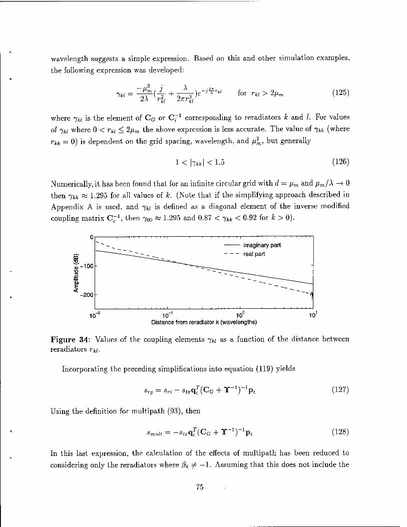
wavelength suggests a simple expression. Based on this and other simulation examples,

the following expression was developed:

Iki 2A [rl + -—^)e-j2?rkl for rkl > 2^ (125)

where 7W is the element of CG or C,"1 corresponding to reradiators k and /. For values

of 'jki where 0 < rki < 2/im the above expression is less accurate. The value of jkk (where

rkk = 0) is dependent on the grid spacing, wavelength, and n2m, but generally

1 < \lkk\ < 1-5 (126)

Numerically, it has been found that for an infinite circular grid with d = /j,m and //m/A —*■ 0

then 7fcfc w 1.295 for all values of k. (Note that if the simplifying approach described in

Appendix A is used, and ^ki is defined as a diagonal element of the inverse modified

coupling matrix C"1, then 700 ~ 1-295 and 0.87 < 7^ < 0.92 for k > 0).

imaginary part

real part

10" 10-1 10° Distance from reradiator k (wavelengths)

10'

Figure 34: Values of the coupling elements 7^ as a function of the distance between reradiators rki.

Incorporating the preceding simplifications into equation (119) yields

srg — sri — stxqj{CG + Y 1) xp£ (127)

Using the definition for multipath (93), then

S-mult = — $tx<ie (CG + T -1\-1, (128)

In this last expression, the calculation of the effects of multipath has been reduced to

considering only the reradiators where ßk ^ — 1. Assuming that this does not include the

75

entire ground grid, then the above expression results in a computational savings.

Defining the dielectric coupling matrix as

(^-(CG + Y-1) (129)

(where the negative sign accounts for the negative sign in (128)), the expression for smuit

can easily be related to the freespace version (54). In this case p£ and qe serve in the

role of transmitter-multipath source and multipath source-receiver attenuation vectors

respectively. The corresponding dielectric earth attenuation function is then given by

ft(p) = zü=e*fi+(!_%»)*).-* (130) A \r2 v A2 727rr3,

where h is the height of the transmitter or receiver antenna (as appropriate) and p = pm

for the transmitter-multipath source path, and p = pr for the multipath source-receiver

path. Compared to the freespace case, for increasing r the amplitude attenuation is a

function of r-2 rather than r_1 and a phase shift of -90° has been introduced.

Continuing the equivalence with the freespace equations, the effective dielectric earth

reradiation coefficient can be defined in terms of the diagonal elements of Ce. The result

is given by

ße =

l+ß (131) 7** + Ikkß - ß

where ß ^ 1. Although slightly complicated looking, since -ykk ~ 1, then ßt w 1 + ß.

As in the case of the definitions developed in the previous section for terrain and vege-

tation features, the definitions for the attenuation function pc(r) and effective reradiation

coefficient ßt developed here can be used in place of the corresponding freespace defini-

tions to implement any of the methods described in Sections 2.0 or 3.0. There is, however,

a slight problem with the computation of the off-diagonal elements of the the dielectric

coupling matrix. For example, making the appropriate substitutions in (50) yields

ck, = Pm(ru) for k^l, M = l,2,3,...,iV (132)

76

Since the ground grid reradiators are at the same height (h = 0), the result is cM - 0 which

contradicts the result computed from (125) using the fact that cki = -7^. Fortunately,

this problem is easily remedied by setting h = -fim/2 in which case (132) becomes a very

good approximation for (130).

In comparing the effects of variations in elevation to variations in the electrical prop-

erties of the earth, the effects are remarkably similar, especially when path losses (or

amplitude attenuations) are considered. The main difference being that the factor 2yftz

in the elevation case has been replaced by -fi. This difference, however, means that

for similarly sized features (as measured on the X-Y plane), elevation effects would be

expected to dominate, particularly when z > ///2v/7r.

77

5.0 SUMMARY OF MULTIPATH EQUATIONS

The multipath models developed in this report are based on representing multipath

sources by collections of reradiators. This was shown to lead to the expression

Smult - StxqlC^Pv (133)

where smuH is the multipath signal picked up by the receiving antenna, stx is the trans-

mitted signal amplitude (measured at the transmitting antenna), pu is the transmitter-

reradiator complex attenuation vector, q„ is the rerdiator-receiver complex attenuation

vector, and C„ is the reradiator coupling matrix. The elements of the attenuation vectors

are defined by

Pk = -PvmiXak) (134)

and

qk = pur(rbk) (135)

respectively, and the elements of the coupling matrix are defined by

' pvm{rki) for k / /

Ckl = \ -1_

. ßvk

(136)

for k — I

The definition of the attenuation functions /w(-), P*r(-), and the reradiation coeffi-

cient ßuk is dependent on the propagation conditions. The three conditions considered in

this report were: free space propagation, propagation over ground with vegetation and

terrain features, and propagation over a flat ground with varying electrical properties

(nonhomogeneous dielectric earth). To distinguish these three conditions, the subscript

v is replaced by a, z, and e accordingly. The definitions appropriate to each propagation

condition are given in the next three subsections.

78

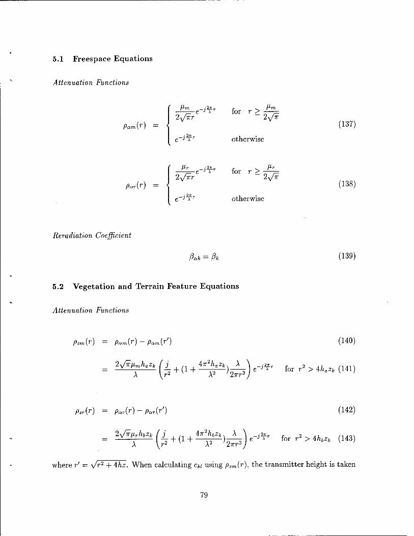
5.1 Freespace Equations

Attenuation Functions

Pam{r)

P-m _,-2a

2^v

= 3 X r

JAr for r > A*n

20F

otherwise

(137)

Par{r) = <

Pr _7-22L,

2^r

.•2TT -J—r

for r > A«r

2^H

otherwise

(138)

Reradiation Coefficient

ßak = ßk (139)

5.2 Vegetation and Terrain Feature Equations

Attenuation Functions

pzm(r) = pam(r) - pam(r') (140)

2yft\xmhazk (j 4n2hazk A \ -^ 2. n /1/M\

P*r(r) = Par(r) - Par(r') (142)

2^firhtZk ( j , 4Tr2hbZk A \ -22T

A + (1 + A2 y27rr3 e"J-r for r2 > 4/^fc (143)

where r' = v^2 + 4/iz. When calculating c^/ using pzm{r), the transmitter height is taken

79

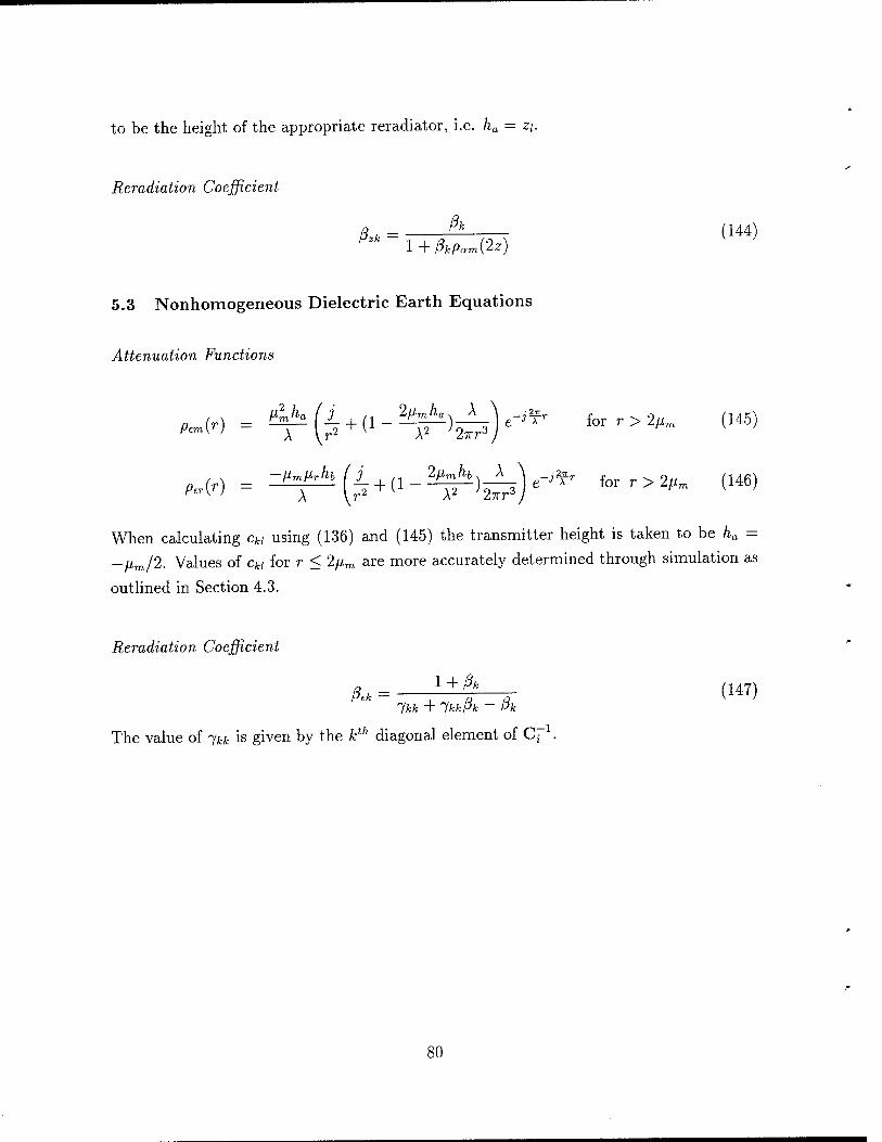
to be the height of the appropriate reradiator, i.e. ha = z\.

Reradiation Coefficient

ßzk = h (144) 1 + ßkpam(2z)

5.3 Nonhomogeneous Dielectric Earth Equations

Attenuation Functions

A-M = ^ (^ + (1 - ^)^) ^' ** ' > **• <"5>

MO = =*f± (^ + (1 " ^)^) ^ for r > ^ <146>

When calculating cw using (136) and (145) the transmitter height is taken to be ha =

-fim/2. Values of c« for r < 2/iro are more accurately determined through simulation as

outlined in Section 4.3.

Reradiation Coefficient

Ikk + Ikkßk - ßk

The value of jkk is given by the kth diagonal element of Cj

ß* = 1+ßak a (147)

80

6.0 REAL WORLD MODELLING EXAMPLES

In this section, two examples are provided of how the equations and methods developed

in this report can be applied to analysis of the effects of VHF multipath on a terrestrial

path. In these examples measurements from two separate field trials are presented which

clearly show the effects of multipath. These effects are then duplicated by setting up

computer simulations and making the appropriate choices and approximations for the

simulations. In fact, even using some very simplistic approximations to simplify the

processing requirements, some very useful results are developed.

6.1 Example 1

In 1994, field trials were carried out at DREO where a mobile VHF CW transmitter was

set up to travel slowly down a predefined route such as the one shown on the map in Figure

35. The rate of travel of the mobile transmitter was 0.3 m/s covering a total distance of

approximately 160 meters or more. The transmitting frequency used was 62.5 MHz for

a signal wavelength of 4.8m. The receiving system consisted of an eight-channel receiver

connected to an eight-element linear array located at the position marked "Osprey" on

the map. Measurements were made at a rate of 4 samples/second. For this first example,

the results for the route shown in Figure 35 are discussed, and this discussion is restricted

to the measured signal power averaged for all 8 channels which is shown in Figure 36.

The signal-to-noise ratio was sufficiently high that the observed fluctuating behaviour or

power ripple in the signal power was due to spatial effects (multipath), and not temporal

effects, i.e. repeating the experiment produces a nearly identical signal power pattern.

The explanation for the observed ripple in power is relatively simple. As the trans-

mitter moves, the path lengths of the direct path and the secondary paths also change.

Since these paths do not all change at the same rate, the relative phase of the direct

and multipath signals are modified. The resultant amplitude of the composite signal is

affected accordingly. The period of the power ripple, measured in terms of transmitter

distance travelled, is dependent on geometry considerations. Generally multipath sources

nearer the receiver causes power ripple with long periods (transmitter distances of many

wavelengths) while multipath sources close to the transmitter cause power ripples with

periods ranging from very long to very short (on the order of one wavelength or less). In-

dividual multipath sources tend to produce variations whose period is relatively constant

(i.e. constant spatial frequency) except when the transmitter is passing by. Inspection

81

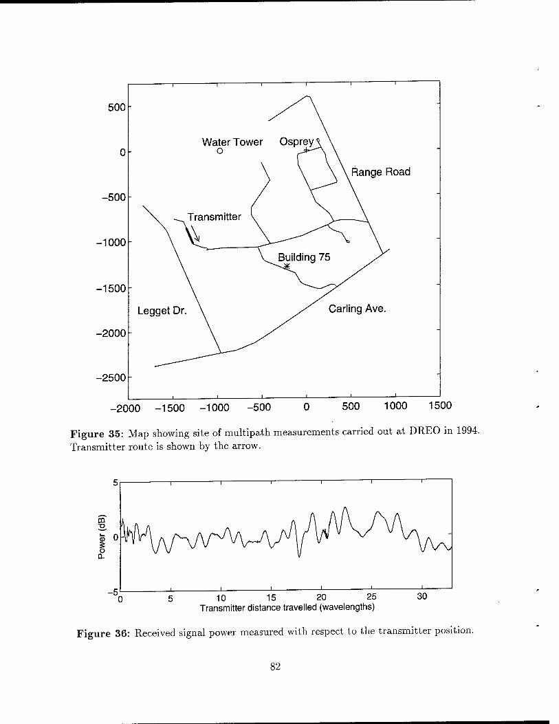
500

0

-500

-1000

-1500

-2000

-2500

Water Tower Osprey' o ' "

Legget Dr

Range Road

Carling Ave.

-2000 -1500 -1000 -500 0 500 1000 1500

Figure 35: Map showing site of multipath measurements carried out at DREO in 1994.

Transmitter route is shown by the arrow.

5 10 15 20 25 Transmitter distance travelled (wavelengths)

30

Figure 36: Received signal power measured with respect to the transmitter position.

82

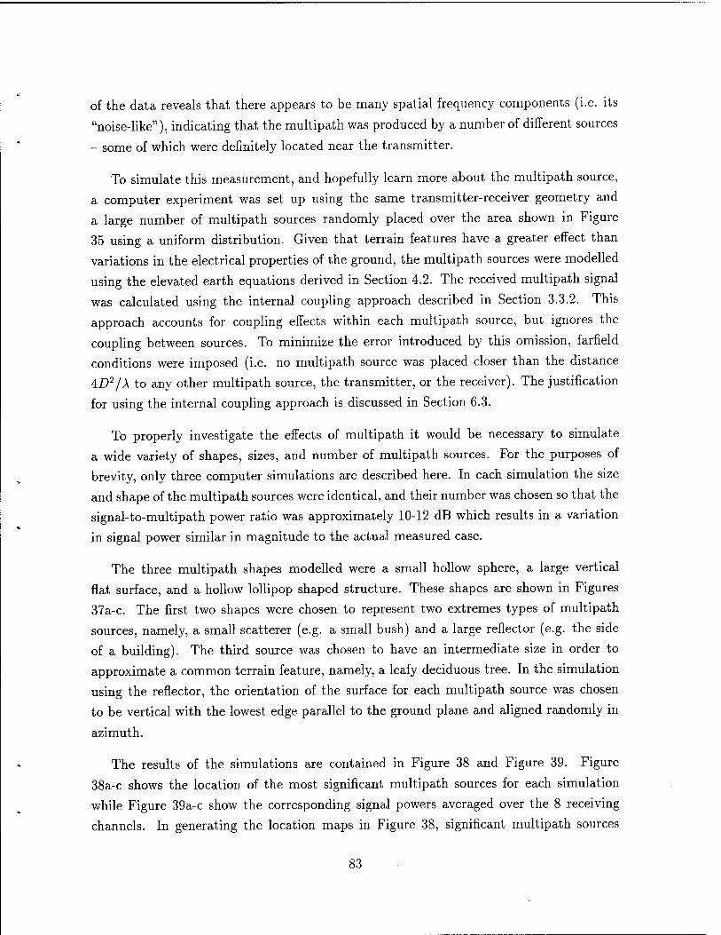
of the data reveals that there appears to be many spatial frequency components (i.e. its

"noise-like"), indicating that the multipath was produced by a number of different sources

- some of which were definitely located near the transmitter.

To simulate this measurement, and hopefully learn more about the multipath source,

a computer experiment was set up using the same transmitter-receiver geometry and

a large number of multipath sources randomly placed over the area shown in Figure

35 using a uniform distribution. Given that terrain features have a greater effect than

variations in the electrical properties of the ground, the multipath sources were modelled

using the elevated earth equations derived in Section 4.2. The received multipath signal

was calculated using the internal coupling approach described in Section 3.3.2. This

approach accounts for coupling effects within each multipath source, but ignores the

coupling between sources. To minimize the error introduced by this omission, farfield

conditions were imposed (i.e. no multipath source was placed closer than the distance

4D2/A to any other multipath source, the transmitter, or the receiver). The justification

for using the internal coupling approach is discussed in Section 6.3.

To properly investigate the effects of multipath it would be necessary to simulate

a wide variety of shapes, sizes, and number of multipath sources. For the purposes of

brevity, only three computer simulations are described here. In each simulation the size

and shape of the multipath sources were identical, and their number was chosen so that the

signal-to-multipath power ratio was approximately 10-12 dB which results in a variation

in signal power similar in magnitude to the actual measured case.

The three multipath shapes modelled were a small hollow sphere, a large vertical

flat surface, and a hollow lollipop shaped structure. These shapes are shown in Figures

37a-c. The first two shapes were chosen to represent two extremes types of multipath

sources, namely, a small scatterer (e.g. a small bush) and a large reflector (e.g. the side

of a building). The third source was chosen to have an intermediate size in order to

approximate a common terrain feature, namely, a leafy deciduous tree. In the simulation

using the reflector, the orientation of the surface for each multipath source was chosen

to be vertical with the lowest edge parallel to the ground plane and aligned randomly in

azimuth.

The results of the simulations are contained in Figure 38 and Figure 39. Figure

38a-c shows the location of the most significant multipath sources for each simulation

while Figure 39a-c show the corresponding signal powers averaged over the 8 receiving

channels. In generating the location maps in Figure 38, significant multipath sources

83

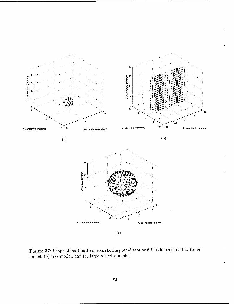
20 s

■»15

e. mo

.§iii|il s§§!!§Ä§§

,o2gg

fill fllllll 111

o°go°go

ills iliilil g°ggg°°

spg S|§§ §§§§ g§g§- gigs llll -g° g°gg.

Y-coordinate (meters) -5 -5 X-coordinate (meters)

Y-coordinate (meters) -10 -10 X-coordinate (meters)

(a) (b)

10

Y-coordinate (meters) X-coordinate (meters)

(c)

Figure 37: Shape of multipath sources showing reradiator positions for (a) small scatterer model, (b) tree model, and (c) large reflector model.

84

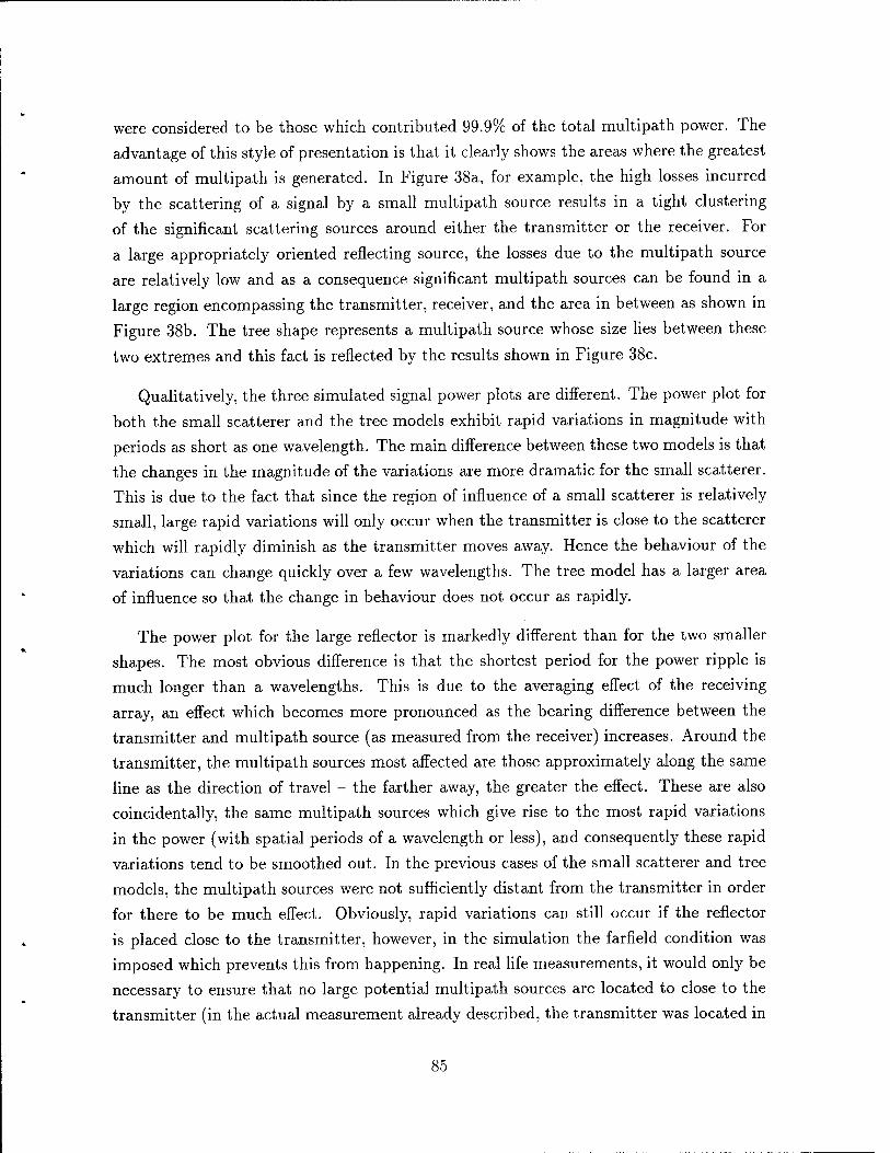
were considered to be those which contributed 99.9% of the total multipath power. The

advantage of this style of presentation is that it clearly shows the areas where the greatest

amount of multipath is generated. In Figure 38a, for example, the high losses incurred

by the scattering of a signal by a small multipath source results in a tight clustering

of the significant scattering sources around either the transmitter or the receiver. For

a large appropriately oriented reflecting source, the losses due to the multipath source

are relatively low and as a consequence significant multipath sources can be found in a

large region encompassing the transmitter, receiver, and the area in between as shown in

Figure 38b. The tree shape represents a multipath source whose size lies between these

two extremes and this fact is reflected by the results shown in Figure 38c.

Qualitatively, the three simulated signal power plots are different. The power plot for

both the small scatterer and the tree models exhibit rapid variations in magnitude with

periods as short as one wavelength. The main difference between these two models is that

the changes in the magnitude of the variations are more dramatic for the small scatterer.

This is due to the fact that since the region of influence of a small scatterer is relatively

small, large rapid variations will only occur when the transmitter is close to the scatterer

which will rapidly diminish as the transmitter moves away. Hence the behaviour of the

variations can change quickly over a few wavelengths. The tree model has a larger area

of influence so that the change in behaviour does not occur as rapidly.

The power plot for the large reflector is markedly different than for the two smaller

shapes. The most obvious difference is that the shortest period for the power ripple is

much longer than a wavelengths. This is due to the averaging effect of the receiving

array, an effect which becomes more pronounced as the bearing difference between the

transmitter and multipath source (as measured from the receiver) increases. Around the

transmitter, the multipath sources most affected are those approximately along the same

line as the direction of travel - the farther away, the greater the effect. These are also

coincidentally, the same multipath sources which give rise to the most rapid variations

in the power (with spatial periods of a wavelength or less), and consequently these rapid

variations tend to be smoothed out. In the previous cases of the small scatterer and tree

models, the multipath sources were not sufficiently distant from the transmitter in order

for there to be much effect. Obviously, rapid variations can still occur if the reflector

is placed close to the transmitter, however, in the simulation the farfield condition was

imposed which prevents this from happening. In real life measurements, it would only be

necessary to ensure that no large potential multipath sources are located to close to the

transmitter (in the actual measurement already described, the transmitter was located in

85

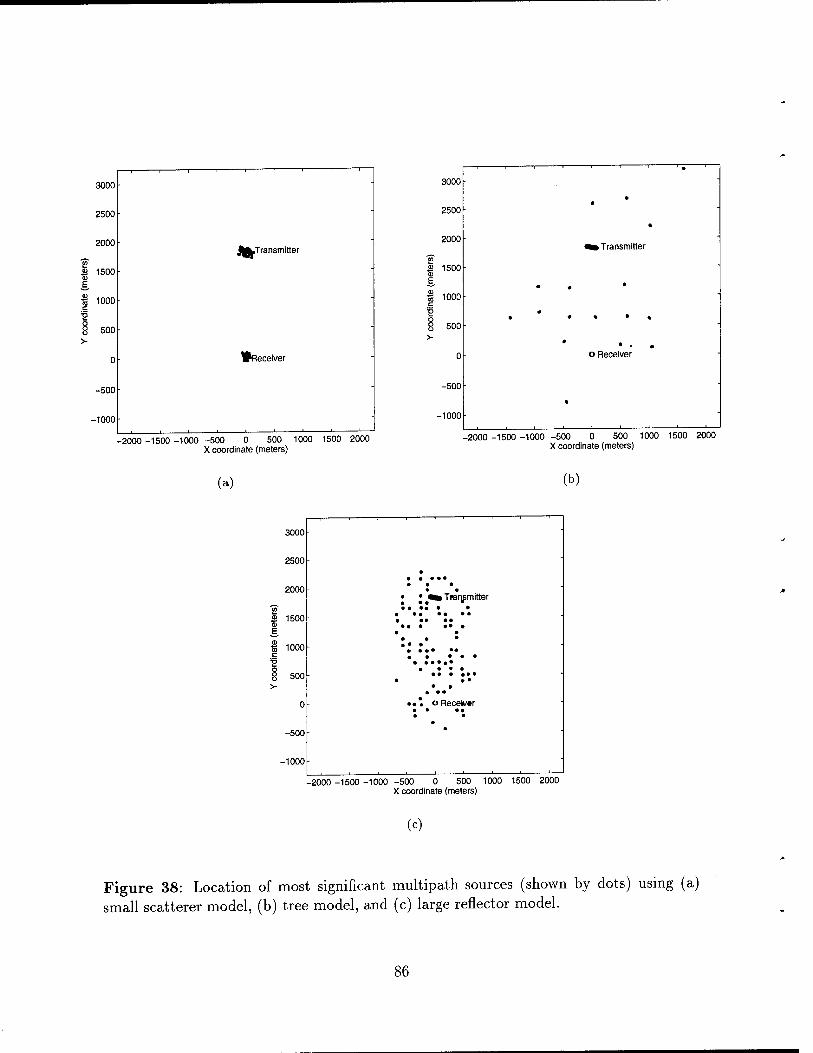
3000

2500

2000 J^Transmitter

(met

ers

o

o

Ü 1000 c

§ 500 >-

0 ^Receiver

-500 -

-1000

3000

2500

2000

S 1500 ® E.

1 1000 c

I 500

-500-

-1000

i Transmitter

o Receiver

-2000 -1500 -1000 -500 0 500 1000 1500 2000 X coordinate (meters)

-2000 -1500 -1000 -500 0 500 1000 1500 2000 X coordinate (meters)

(a) (b)

3000 ■

2500 •

- • • • ••

«II III • • • • ^Tfaqpmitter • • • •• • •

- 1500 • • •• • • • •• • • • • • • 1000 • • • • • • • •• ■

• • • • • • • • •

500 • •• • ••• • • • • • • • 0 • 4 • o Receiv«r

i • •• ■ • • -500 ■

-1000 " ■

-2000 -1500 -1000 -500 0 500 1000 1500 2000 X coordinate (meters)

(c)

Figure 38: Location of most significant multipath sources (shown by dots) using (a) small scatterer model, (b) tree model, and (c) large reflector model.

86

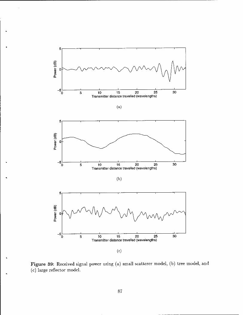
10 15 20 25 Transmitter distance travelled (wavelengths)

30

(a)

10 15 20 25 Transmitter distance travelled (wavelengths)

30

(b)

10 15 20 25 Transmitter distance travelled (wavelengths)

30

(c)

Figure 39: Received signal power using (a) small scatterer model, (b) tree model, and

(c) large reflector model.

87

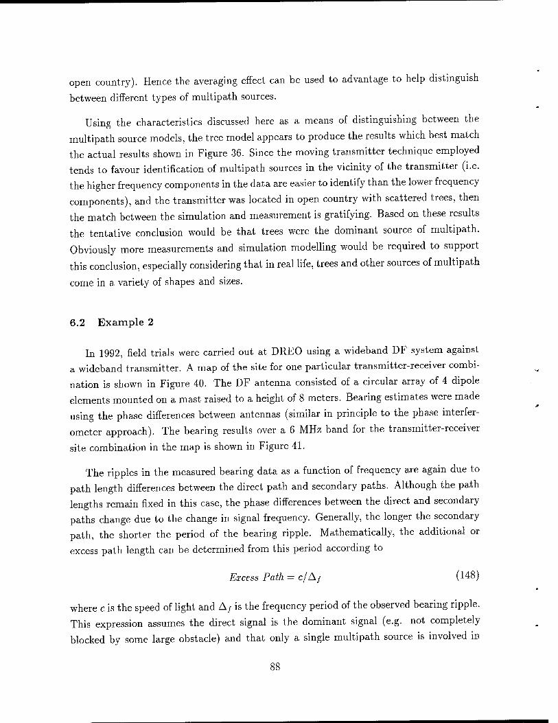
open country). Hence the averaging effect can be used to advantage to help distinguish

between different types of multipath sources.

Using the characteristics discussed here as a means of distinguishing between the

multipath source models, the tree model appears to produce the results which best match

the actual results shown in Figure 36. Since the moving transmitter technique employed

tends to favour identification of multipath sources in the vicinity of the transmitter (i.e.

the higher frequency components in the data are easier to identify than the lower frequency

components), and the transmitter was located in open country with scattered trees, then

the match between the simulation and measurement is gratifying. Based on these results

the tentative conclusion would be that trees were the dominant source of multipath.

Obviously more measurements and simulation modelling would be required to support

this conclusion, especially considering that in real life, trees and other sources of multipath

come in a variety of shapes and sizes.

6.2 Example 2

In 1992, field trials were carried out at DREO using a wideband DF system against

a wideband transmitter. A map of the site for one particular transmitter-receiver combi-

nation is shown in Figure 40. The DF antenna consisted of a circular array of 4 dipole

elements mounted on a mast raised to a height of 8 meters. Bearing estimates were made

using the phase differences between antennas (similar in principle to the phase interfer-

ometer approach). The bearing results over a 6 MHz band for the transmitter-receiver

site combination in the map is shown in Figure 41.

The ripples in the measured bearing data as a function of frequency are again due to

path length differences between the direct path and secondary paths. Although the path

lengths remain fixed in this case, the phase differences between the direct and secondary

paths change due to the change in signal frequency. Generally, the longer the secondary

path, the shorter the period of the bearing ripple. Mathematically, the additional or

excess path length can be determined from this period according to

Excess Path = c/Aj (148)

where c is the speed of light and Af is the frequency period of the observed bearing ripple.

This expression assumes the direct signal is the dominant signal (e.g. not completely

blocked by some large obstacle) and that only a single multipath source is involved in

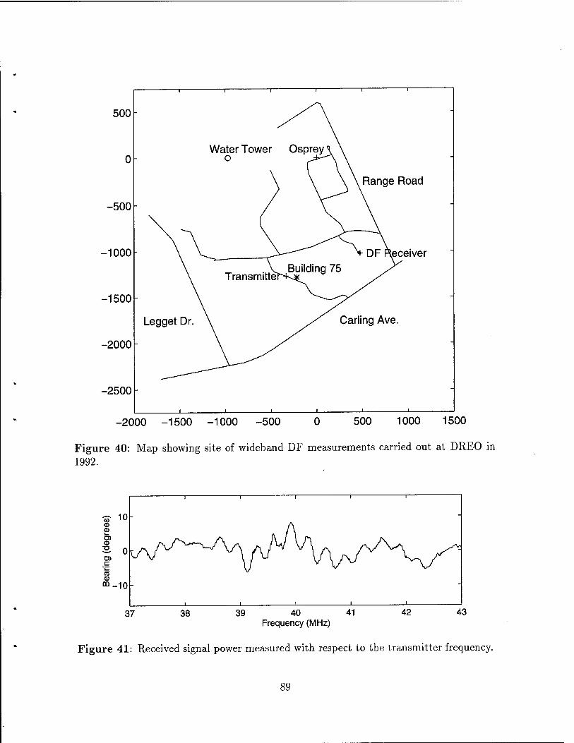
500

i r ' i 1 i i

0 - Water Tower

o Osprey\ \

\ \\ Range Road

-500 - \ \

1000 -— V DF Receiver Building 75 J^

Transmitter

1500 ^-^_^->^

Legget Dr. /S Carling Ave.

2000 - S

2500

i i i i i i

-2000 -1500 -1000 -500 500 1000 1500

Figure 40: Map showing site of wideband DF measurements carried out at DREO in 1992.

37 38 39 40 41 Frequency (MHz)

Figure 41: Received signal power measured with respect to the transmitter frequency.

89

producing the bearing ripple. In Figure 41, the bearing ripple contains several components

with different periods, however one component with a period of 325 kHz is clearly evident.

Assuming this is caused by a single source, then using the above expression, the excess

path length is 923 m.

To simulate the wideband DF measurement, a computer experiment was again setup

employing the same transmitter and DF receiver geometry as the actual measurement.

Using a uniform distribution, multipath sources were spread randomly across the region

encompassing the transmitter and receiver. The density of multipath sources was chosen

to give a signal-to-multipath power ratio of approximately 10 dB. The farfield condition

was again imposed to allow the internal coupling method to be used. Since an excess path

of 923m suggests larger multipath sources, only the tree model and large flat reflecting

surface model were tested in the simulations. The dimensions of the tree model were the

same as before while the flat surface was composed of a 14 x 14 grid of reradiators with

a reradiator spacing of d = 1.5m (instead of a 19 x 19 grid with d = 0.96m). The results

of the simulations are shown in Figure 42.

Comparing the simulation results to the actual measurements reveals that the large

reflecting surface model provides a more realistic simulation, particularly when the bearing

ripple components with short periods are considered. This is in contrast to the results

found in the first example. The reason for this is probably due to the fact that in this

second example the transmitter was located near a number of medium sized buildings,

while in the first example the transmitter was in an open area with a few scattered trees

(the receiver environments were similar in both cases - open field surrounded by groves of

trees). Alternatively, the results of the second example may still indicate that smaller tree

sized objects still dominate, but that the environment does contain a few larger reflectors.

The higher frequency bearing ripple in Figure 41, for example, may have be due to a

single multipath source only. Hence, this suggests that more real measurements would be

required to make a better assessment, and that simulations should include a variety of

multipath models with varying sizes and shapes which have dimensions similar to those

found in the real environment.

6.3 Assumption Verification

In the examples presented in this section, a number of simplifications were used to

reduce the processing. In particular, the farfield condition was introduced to allow the

90

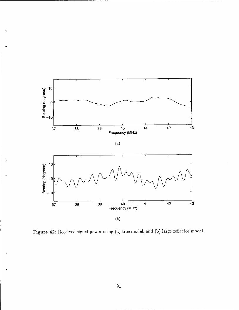
37 38 39 40 41 Frequency (MHz)

42

(a)

37 38 39 40 41 Frequency (MHz)

42

(b)

Figure 42: Received signal power using (a) tree model, and (b) large reflector model.

91

use of the internal coupling method which greatly simplifies processing. This simplification

was therefore based on two assumptions: imposing farfield conditions would not distort

the results, and coupling between multipath sources could be ignored. An important

question when considering the results was were these assumptions valid?

The justification for the farfield assumption was that it was found that for the densities

of multipath sources required to generate a realistic amount of multipath, the average

spacing exceeded the farfield condition. However, in the real world, no such condition

is imposed so that in some situations this could lead to erroneous results. This was

apparent when analyzing the result for Figure 39c where it was previously pointed out

that the farfield condition in conjunction with the averaging of the receive array leads

to a slowly varying signal power plot - a result that would only occur in real life if the

multipath sources were some distance from the transmitter. Had the transmitter been

located close to a large grove of trees, the power measurements could have easily exhibited

rapid variations similar to those generated by smaller multipath sources, leading to the

false conclusion that the multipath effects were generated by isolated trees.

Previously it was found (Section 3.3.3) that coupling between sources could be ignored

if farfield condition were met. As a precaution and where possible, simulations were also

carried out using the full method and the multipath source coupling method. In all cases

the shape of the power plots were virtually indistinguishable from the shape generated

using the internal coupling method. Generally, the received multipath power was slightly

higher (1 dB or less) for internal coupling method than the other two methods. Since the

shape of the signal power plots was of most interest, the small error in received multipath

power was inconsequential.

From this discussion, it is clear that under the conditions specified, the assumptions

used for the simulations in the examples were reasonable. It is also equally clear that

the success of any simulation is highly dependent on the validity of the underlying as-

sumptions. Hence a very important part of the modelling process necessarily includes

verification of the underlying assumptions

92

7.0 CONCLUSIONS

In this report, a new approach to modelling propagation effects that occur for ter-

restrial paths was introduced. The main motivation for developing this approach was

to provide a means of investigating effects observed in VHF radio direction finding mea-

surements for terrestrial paths. Particularly the effects due to multipath caused by the

transmitted radio signal being reradiated, reflected, or diffracted off of bushes, trees,

forests, buildings, hills, etc.

The new approach is based on representing the terrain and vegetation, which effect

the signal path, by a large number of small (relative to the signal wavelength) isotropic

reradiators. In this way it incorporates some of the sophistication found in the more com-

plex and computationally intensive electromagnetic methods commonly used for antenna

modelling. This degree of sophistication is necessary to help understand the fine scale

effects observed in actual measured data (e.g. rapid changes in received signal amplitude

as the transmitter is moved distances of as little as one wavelength). Current propagation

models tend to overlook these fine scale effects.

Despite being simpler than electromagnetic methods, the computational requirements

for the new approach can easily exceed the abilities of most present day computers for

problems involving typical military signal paths. However, various simplifications can

be employed to greatly simplify the computations depending on the complexity of the

terrain and vegetation, and the qualities of the model data that are of most interest. For

example, a flat homogeneous ground with only a few terrain features can be modelled by

subdividing the terrain features into collections of isotropic reradiators. The effect of the

rest of the ground can then be directly incorporated into the calculations without having

to subdivide it as well. If these features are far enough apart, it may be possible to ignore

the coupling interaction between these features. The calculations can then be done by

examining one feature at a time and using superposition to get the final results.

Using some of these simplifications, it was shown that the new method was able to

produce results which were comparable to real world examples. In addition by making

suitable adjustments to the simulation in terms of the number of sources of multipath,

their size and shape, the best results were achieved when the adjusted parameters mostly

matched those of the corresponding features in the real world.

For complex environments (lots of obstacles in the signal path such as bushes, trees,

etc.), coupling effects become more and more important. Under these conditions, the

93

number of features to be modelled and the fact that coupling effects need to be considered,

would likely make the computations for the new method prohibitive. Hence more work

will be required in simplifying the computations if these environments are to be analyzed.

In general, the new method provides a means of better understanding the effects due

to multipath observed in terrestrial VHF signal problems. In particular, understanding

the effects due to small changes in the position of the transmitter or receiver, or small

changes in the transmission frequency. It also opens up the possibility of testing and

developing new VHF DF algorithms which are better able to deal with the VHF multipath

environment than current approaches. Additionally, it will also be possible to test the

usefulness of different DF site calibration methods, and possibly develop improved ones.

94

REFERENCES

[1] Read, W., "The Effects of the Environment on an Experimental VHF Radio Direc-

tion Finding Antenna System", Defence Research Establishment Ottawa, Report No.

1226, August 1994.

[2] Read, W.,J„L„ "Measurements of Multipath and its Effects on Terrestrial VHF

Radio Direction Finding", DREO Report xxxx, February 1996.

[3] Whitteker, J.H., "Ground Wave and Diffraction", Propagation Modelling and De-

cision Aids for Communications, Radar and Navigation Systems, AG ART) Lecture

Series 196, pp. 2A-1 to 2B-14, September 1994.

[4] Born, M., and Wolf, E., Principles of Optics, Pergamon Press, Oxford, England, p.

132, 1965.

[5] "Report on VHF DF Super-resolution Field Trials held at Defence Research Estab-

lishment Ottawa", TTCP Report by Subgroup Q, Technical Panel QTP-18, Septem-

ber 1994, CONFIDENTIAL.

[6] "Navaids and Avionics Enroute Systems, Doppier VHF/DF, Site Selection", Publi-

cation No. C4-2VHF/DF-3, Telecommunications and Electronics Branch, Transport

Canada, March 1, 1976.

[7] Kraus, J.D., Antennas, McGraw-Hill Book Company, New York, U.S.A, Chapter

3.11, 1950.

[8] Beckmann, P., and Spizzichino, A., The Scattering of Electromagnetic Waves from

Rough Surfaces, Artech House, Inc., Norwood, MA, U.S.A, Chapters 2.2, 1987.

[9] Linear Systems, Thomas Kailith, Editor, Prentice-Hall, Inc, Englewood Cliffs, N.J.,

U.S.A, pp. 655-656, 1980.

[10] Shigekazu, S., A Basic Atlas of Radio-Wave Propagation, John Wiley and Sons, 1987.

[11] Wolfram, S., Mathematica: A System for Doing Mathematics by Computer, Addison-

Wesley Publishing Company Inc., Redwood City, California, 1991.

REF-1

APPENDIX

A.O CIRCULAR GROUND GRID CALCULATIONS

In this section the analysis focuses on reducing the amount of processing required

to perform ground grid calculations by using a circular grid of reradiators. This analysis

is limited to the case where the transmitter is positioned above the center of the grid, and

reradiators at the same radius from the center all have the same value for ß.

Consider a circular grid of reradiators such as the one shown in Figure 31. Num-

bering the reradiators in a clockwise manner spiraling outwards, then equation (47) can

be re-expressed as,

_ 3 19 37

stxpm(r0) = -^- + SiJ2pm(ru) + s2J2p^(r^) + s^ Y, Pm(ru) + - Pi i=2 i=8 i=20

(_i 7 \ 19 37

-5- + X)/>m(r2;) + s2Y,Pm(r2i) + s3 J2 P™{r2i) + - Pi i=3 / »=8 i=20

7 / _Y 19 \ 37

-stxpm(r2) = s0pm(r8o) + SiY,Pm(r8i) + s2 I — + J2pm(rsi) I + -S3 Yl Pm{r&i) + ••• t'=2 V ^8 t*=9 / i=20

etc. (A.l)

The above expression can also be expressed in matrix form as

where pc is the transmitter-grid attenuation vector with elements defined by

Pk = -pm(rk) (A.3)

s5 is the reradiated grid signal with elements s0,Si, s2,..., and Cc is the modified coupling

matrix with elements given by

n2

Ckn = Yl Pmirini) for k^n (A.4) i=nj

A-l

APPENDIX

and _1 n2

Cnn = ö- + E /°m(rnii) (A.5) All j=ni+l

with iki representing the lowest numbered reradiator in the kth ring, and nx and n2 repre-

senting the lowest and highest numbered reradiators in the nth ring respectively. Finally,

to solve for the reradiated signal s5, equation (A.2) is rearranged to get

s5 = stxC;lpc (A.6)

Suppose now, that the receiver is colocated with the transmitter. The signal

received from the grid can be found by summing the contributions from the individual

reradiators. Mathematically,

7 19

Sgrid = SOpmini) + SlJ2 Prn(rbi) + S2Ys P™(rbi) + - (A-7) t'=2 i-S

where rbk is the distance from the receiver to the kth reradiator. Since the distance for

every reradiator in the nth ring is given by rn then this expression can be simplified to

Sgrid = sopm{r0) + 5i6pm(ri) + s212pm(r2) + ... (A.8)

and using the matrix equations developed earlier, this can be rewritten as

Sgrid = SteqjTC^Pc (A.9)

where qc is the grid-receiver attenuation vector with elements defined by

qk = Kpm(rk) (A.10)

and where K is the number of reradiators in the kth ring (K « 2irk).

A-2

UNCLASSIFIED SECURITY CLASSIFICATION OF FORM

(highest classification of Title. Abstract, Keywords)

-99-

DOCUMENT CONTROL DATA (Security classification of titla, body of abstract and indexing annotation mutt ba antarad whan tha ovarall documant is classifiad)

1. ORIGINATOR (the name and address of the organization prepving the document Organizations for whom the document was prepared, e.g. Establishment sponsoring a contractor's report, or tasking agency, are entered in section 8.) DEFENCE RESEARCH ESTABLISHMENT OTTAWA NATIONAL DEFENCE SHIRLEYS BAY, OTTAWA, ONTARIO K1A 0Z4 CANADA

2. SECURITY CLASSIFICATION (overall security classification of the document including special warning terms if applicable)

UNCLASSIFIED

3. TITLE (the complete document title as indicated on the title page. Its classification should be indicated by the appropriate abbreviation (S.C or U) in parentheses after the title.)

MULTIPATH MODELLING FOR TERRESTRIAL VHF RADIO DIRECTION FINDING (U)

4. AUTHORS (Last name, first name, middle initial) READ, WILLIAM J.L.

5. DATE OF PUBLICATION (month and year of publication of document)

DECEMBER 1996

6a. NO. OF PAGES (total containing information. Include Annexes, Appendices, etc.)

94

6b. NO. OF REFS (total cited in document)

11

7. DESCRIPTIVE NOTES (the category of the document, e.g. technical report, technical note or memorandum. If appropriate, enter the type of report, e.g. interim, progress, summary, annual or final. Give the inclusive dates when a specific reporting period is covered.)

DREO REPORT

SPONSORING ACTIVITY (the name of the department project office or laboratory sponsoring the research and development Include the address.)

DEFENCE RESEARCH ESTABLISHMENT OTTAWA, NATIONAL DEFENCE dHTRTVVC; BAY, OTTAWA, DTJTABTn K1A 07,4 (1ANAT)A

9a. PROJECT OR GRANT NO. (if appropriate, the applicable research and development project or grant number under which the document was wrinen. Please specify whether project or grant)

5BD12

10a. ORIGINATOR'S DOCUMENT NUMBER (the official document number by which the document is identified by the originating activity. This number must be unique to this document)

DREO REPORT 1300

9b. CONTRACT NO. (if appropriate, the applicable number under which the document was wrinen)

10b. OTHER DOCUMENT NOS. (Any other numbers which may be assigned this document either by the originator or by the sponsor)

1 1. DOCUMENT AVAILABILITY (any limitations on further dissemination of the document, other than those imposed by security classification)

X) Unlimited distribution ) Distribution limited to defence departments and defence contractors; further distribution only as approved ) Distribution limited to defence departments and Canadian defence contractors; further distribution only as approved

> Distribution limited to government departments and agencies; further distribution only as approved

) Distribution limited to defence departments; further distribution only as approved

) Other (please specify):

12. DOCUMENT ANNOUNCEMENT (any limitation to the bibliographic announcement of this document This will normally correspond to the Document Availabilty (11). However, where further distribution (beyond the audience specified in 11) is possible, a wider announcement audience may be selected.)

UNLIMITED

UNCLASSIFIED

SECURITY CLASSIFICATION OF FORM

OCD03 2/06/87

UNCLASSIFIED SECURITY CLASSIFICATION OF FORM

13. ABSTRACT ( . brie« and tactual summary o« the document It rr*y also appear elsewhere n ^XLlTrZcS^'oi V desirable ttai the abstract of classified documents be unclassified. tach tngr«h of the abstracshaleg""'**> 'nd '«t,on «™ security classification of the information in the paragraph (unless the document itself is unclassified) represented as <S). «3. or IUI. It is not necessary to include here abstracts in both offieal languages unless the text is bilingual).

(U) This report details the development of computer models to investigate and explain the effects of multipath on VHF radio direction finding (DF). The motivation for this development was to help explain the large and small scale multipath effects which occur for changes in transmitter and receiver position, or for changes in frequency. Particularly important in the analysis of current wide and narrow band DF approaches and the development of better ones. The new approach is based on representing the terrain and vegetation, which effect the signal path, by a large number of small (relative to the signal wavelength) isotropic reradiators. Polarization effects are not accounted for Although this kind of approach can quickly become a computationally daunting task, a number oi simplifications are introduced which greatly simplify the calculations. Two examples have been included illustrating the use of the proposed approach in the analysis and modelling real world

measurements.

14 KEYWORDS. DESCRIPTORS or IDENTIFIERS (technically meaningful terms or short phrases that characterize a document and coulcI be ' helpful in cataloguing the document They should be selected so that no security etolfi*ion ii required IdeMfierfcsw:h « equ.w»nt

model designation, trade name, military project code name, geographic location may also be included. If poisibe keywo ds sh,oud be «,e«ed

from a published thesaurus, e.g. Thesaurus of Engineering and Scientific Terms (TEST) and that thesaurus-identified. If it is not possible to select indexing terms which are Unclassified, the classification of each should be indicated as with the title.)

MULTIPATH TRANSMISSION VHF DIRECTION FINDING PROPAGATION N-CHANNEL BEAM FORMING SIMULATION COMPUTER MODELS ANTENNA ARRAYS

TTNHT.ASSTFTED

SECURITY CLASSIFICATION OF FORM