Embed Size (px)
Citation preview

E l e c t r o n ic
Jo
ur n a l
of
Pr
o b a b i l i t y
Electron. J. Probab. 19 (2014), no. 121, 1–64.ISSN: 1083-6489 DOI: 10.1214/EJP.v19-3621
Spatial evolutionary gameswith small selection coefficients*
Rick Durrett†
Abstract
Here we will use results of Cox, Durrett, and Perkins [56] for voter model perturbationsto study spatial evolutionary games on Zd, d ≥ 3 when the interaction kernel is finiterange, symmetric, and has covariance matrix σ2I. The games we consider have payoffmatrices of the form 1+ wG where 1 is matrix of all 1’s and w is small and positive.Since our population size N =∞, we call our selection small rather than weak whichusually means w = O(1/N).
The key to studying these games is the fact that when the dynamics are suitablyrescaled in space and time they convergence to solutions of a reaction diffusionequation (RDE). Inspired by work of Ohtsuki and Nowak [28] and Tarnita et al [35, 36]we show that the reaction term is the replicator equation for a modified game matrixand the modifications of the game matrix depend on the interaction kernel onlythrough the values of two or three simple probabilities for an associated coalescingrandom walk.
Two strategy games lead to an RDE with a cubic nonlinearity, so we can describethe phase diagram completely. Three strategy games lead to a pair of coupled RDE,but using an idea from our earlier work [59], we are able to show that if there is arepelling function for the replicator equation for the modified game, then there iscoexistence in the spatial game when selection is small. This enables us to provecoexistence in the spatial model in a wide variety of examples including the behaviorof four evolutionary games that have recently been used in cancer modeling.
Keywords: replicator equation; PDE; Lyapunov function ; cancer models.AMS MSC 2010: 60K35 ; 92D15.Submitted to EJP on June 24, 2014, final version accepted on December 27, 2014.Supersedes arXiv:1406.5876.
*Partially supported by NSF grant DMS 1305997 and NIH grant R01-GM096190.†Duke University, USA. E-mail: [email protected]

Spatial evolutionary games
1 Introduction
Game theory was invented by John von Neumann and Oscar Morgenstern [1] to studystrategic and economic decisions of humans. Maynard Smith and Price [2], introducedthe concept into ecology in order to explain why conflicts over territory between maleanimals of the same species are usually of the “limited war” type and do not causeserious damage. As formulated in John Maynard Smith’s classic book, [3], this is the
Example 1.1. Hawks-Doves game. When a confrontation occurs, Hawks escalate andcontinue until injured or until an opponent retreats, while Doves make a display of forcebut retreat at once if the opponent escalates. The payoff matrix is
Hawk DoveHawk (V − C)/2 V
Dove 0 V/2
Here V is the value of the resource, which two doves split, and C is the cost of compe-tition. There are two conventions in the literature for the interpretation of the payoffmatrix. Here we are using the one in which the first row gives the payoffs for the Hawkstrategy based on the opponent’s strategy choice.
If we suppose that C > V then a frequency p = V/C of Hawks in the populationrepresents an equilibrium, since in this case each strategy has the same payoff. Theequilibrium is stable. If the frequency of the Hawk strategy rises to p > V/C then theHawk strategy has a worse payoff than the Dove strategy so its frequency will decrease.
Axelrod and Hamilton [4], see also [5], studied the evolution of cooperation byinvestigating
Example 1.2. Prisoner’s dilemma. Rather than formulate this in terms of prisonersdeciding whether to confess or not, we consider the following game between cooperatorsC and defectors D. Here c is the cost that cooperators pay to provide a benefit b to theother player.
C DC b− c −cD b 0
If b > c > 0 then the defection dominates cooperation, and, as we will see, altruisticcooperators are destined to die out in a homogeneously mixing population. This isunfortunate since the (D,D) payoff is worse than (C,C) payoff. Nowak and May [11, 12]found an escape from this dilemma by showing that spatial structure allowed persistenceof cooperators. Huberman and Glance [13] suggested that this was an artifact of thesynchronous deterministic update rule, but later work [14, 15] showed that the samephenomena occurred for asynchronous stochastic updates.
There are many examples of 2 × 2 games with names like Harmony, the SnowdriftGame, and the Battle of the Sexes, see e.g., [21], but as we will see in Section 6 thereare really only 3 (or 4) examples. To complete the set of possibilities, we now consider
Example 1.3. Stag Hunt. The story of this game was briefly described by Rousseau inhis 1755 book A Discourse on Inequality. If two hunters cooperate to hunt stag (an adultmale deer) then they will bring home a lot of food, but there is practically no chance ofbagging a stag by oneself. If both hunters go after rabbit they split what they kill. Anexample of a game of this type is:
Stag HareStag 3 0Hare 2 1
EJP 19 (2014), paper 121.Page 2/64
ejp.ejpecp.org

Spatial evolutionary games
In this case if the two strategies have frequency p = 1/2 in the population, then the twostrategies have equal payoffs. If the frequency of the stag strategy rises to p > 1/2 thenit has the better payoff and will continue to increase so this is an unstable equilibrium.
In the forty years since the pioneering work of Maynard Smith and Price [2] evolu-tionary game theory has been used to study many biological problems. For surveys see[6]–[10]. This is natural because evolutionary game theory provides a general frame-work for the study of frequency dependent selection. In the references we have listedrepresentative samples of work of this type, [16]–[37]. There are literally hundreds ofreferences, so we have restricted our attention to those that are the most relevant to ourinvestigations.
In recent years, evolutionary game theory has been applied to study cancer. Thisprovides an important motivation for our work, so we will now consider four examplesbeginning with one first studied by Tomlinson [48].
Example 1.4. Three species chemical competition. In this system, there are cellsof three types.
1. Ones that Produce a toxic substance, and are sensitive to toxins produced by othercells.
2. Others that are Resistant to the toxin, but do not produce it.
3. Wild type cells that are Sensitive to the toxin but do not produce it.
Based on the verbal description, Tomlinson wrote down the following game matrix.
P R S
P z − e− f + g z − e z − e+ g
R z − h z − h z − hS z − f z z
Here, and in what follows it is sometimes convenient to number the strategies 1 = P ,2 = R and 3 = S. For example, this makes it easier to say that Gij is the payoff to aplayer who plays strategy i against an opponent playing strategy j. Taking the rows inreverse order, z is the baseline fitness while f is the cost to a sensitive cell due to thepresence of the toxin. The cost of resistance to the toxin is h. In top row e is the cost ofproducing the toxin, and g is advantage to a producer when it interacts with a sensitivecell.
It is interesting to note that in the same year [48] was published, Durrett and Levin[62] used a spatial model to model the competition two strains of E. coli, whose behaviorscorrespond to strategies P , R, and S above. In their model, there are also empty cells(denoted by 0). Thinking of a petri dish, their system takes place on the two dimensionallattice with the following dynamics.
• Individuals of type i > 0 give birth at rate βi with their offspring sent to a sitechosen at random from the four nearest neighbors of x. If the site is occupiednothing happens.
• Each species dies at rate δi due to natural causes, while type 3’s die at an additionalrate γ times the fraction of neighbors of type 1 due to the effect of colicin.
Example 1.5. Glycolytic phenotype. It has been known for some time that cancercells commonly switch to glycolysis for energy production. Glycolysis is less efficientthan the citrate cycle in terms of energy, but allows cell survival in hypoxic environ-ments. In addition, cells with glycolytic metabolism can change the pH of the localmicroenvironment to their advantage.
EJP 19 (2014), paper 121.Page 3/64
ejp.ejpecp.org
Spatial evolutionary games
The prevalence of glycolytic cells in invasive tumor suggests that their presence couldbenefit the emergence of invasive phenotypes. To investigate this using evolutionarygame theory, Basanta et al [45] considered a three strategy game in which cells areinitially characterized as having autonomous growth (AG), but could switch to glycolysisfor energy production (GLY ), or become increasing mobile and invasive (INV ). Thepayoff matrix for this game, which is the transpose of the one in their Table 1, is:
AG INV GLY
AG 12 1 1
2 − nINV 1− c 1− c
2 1− cGLY 1
2 + n− k 1− k 12 − k
Here c is the cost of mobility, k is the cost to switch to glycolysis, and n is the detrimentfor nonglycolytic cell in glycolytic environment, which is equal to the bonus for aglycolytic cell. Recently this system has been extended to a four player game by addingan invasive-glycolytic strategy, see [43].
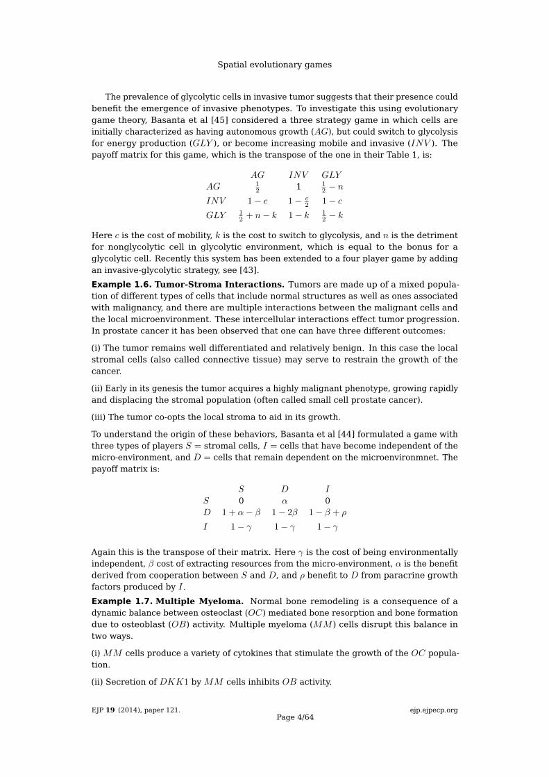
Example 1.6. Tumor-Stroma Interactions. Tumors are made up of a mixed popula-tion of different types of cells that include normal structures as well as ones associatedwith malignancy, and there are multiple interactions between the malignant cells andthe local microenvironment. These intercellular interactions effect tumor progression.In prostate cancer it has been observed that one can have three different outcomes:
(i) The tumor remains well differentiated and relatively benign. In this case the localstromal cells (also called connective tissue) may serve to restrain the growth of thecancer.
(ii) Early in its genesis the tumor acquires a highly malignant phenotype, growing rapidlyand displacing the stromal population (often called small cell prostate cancer).
(iii) The tumor co-opts the local stroma to aid in its growth.
To understand the origin of these behaviors, Basanta et al [44] formulated a game withthree types of players S = stromal cells, I = cells that have become independent of themicro-environment, and D = cells that remain dependent on the microenvironmnet. Thepayoff matrix is:
S D I
S 0 α 0D 1 + α− β 1− 2β 1− β + ρ
I 1− γ 1− γ 1− γ
Again this is the transpose of their matrix. Here γ is the cost of being environmentallyindependent, β cost of extracting resources from the micro-environment, α is the benefitderived from cooperation between S and D, and ρ benefit to D from paracrine growthfactors produced by I.
Example 1.7. Multiple Myeloma. Normal bone remodeling is a consequence of adynamic balance between osteoclast (OC) mediated bone resorption and bone formationdue to osteoblast (OB) activity. Multiple myeloma (MM ) cells disrupt this balance intwo ways.
(i) MM cells produce a variety of cytokines that stimulate the growth of the OC popula-tion.
(ii) Secretion of DKK1 by MM cells inhibits OB activity.
EJP 19 (2014), paper 121.Page 4/64
ejp.ejpecp.org

Spatial evolutionary games
OC cells produce osteoclast activating factors that stimulate the growth of MM cellswhere as MM cells are not effected by the presence of OB cells. These considerationslead to the following game matrix. Here, a, b, c, d, e > 0.
OC OB MM
OC 0 a b
OB e 0 −dMM c 0 0
For more on the biology, see Dingli et al. [46].
A number of other examples have been studied. Tomlinson and Bodmer [49] studiedgames motivated by angiogenesis and apototsis. See Basanta and Deutsch [40] for asurvey of this and other early work. Swierniak and Krzeslak’s survey [47] contains thefour examples we have covered here, as well as a number of others.
2 Overview
In a homogeneously mixing population, xi = the frequency of players using strategy ifollows the replicator equation
dxidt
= xi(Fi − F )
where Fi =∑j Gi,jxj is the fitness of strategy i and F =
∑i xiFi is the average fitness.
Twenty years ago, Durrett and Levin [16] studied evolutionary games and formulatedrules for predicting the behavior of spatial models from the properties of the mean-fielddifferential equations obtained by supposing that adjacent sites are independent. See[60] for an overview of this approach. Our main motivation for revisiting this questionis that the recent work of Cox, Durrett, and Perkins [56] allows us to turn the heuristicprinciples of [16] into rigorous results for evolutionary games with matrices of the formG = 1 + wG, where w > 0 is small, and 1 is a matrix that consists of all 1’s.
We will study these games on Zd where d ≥ 3 and the interactions between anindividual and its neighbors are given by an irreducible probability kernel p(x) on Zd
with p(0) = 0 that is finite range, symmetric p(x) = p(−x), and has covariance matrixσ2I. To describe the dynamics we let ξt(x) be the strategy used by the individual at x attime t and
ψt(x) =∑y
G(ξt(x), ξt(y))p(y − x)
be the fitness of x at time t. In Birth-Death dynamics, site x gives birth at rate ψt(x) andsends its offspring to replace the individual at y with probability p(y − x). In Death-Birthdynamics, the individual at x dies at rate 1, and replaces itself by a copy of the one at ywith probability proportional to p(y − x)ψt(y).
When w = 0 either version of the dynamics reduces to the voter model, a system inwhich each site at rate 1 changes its state to that of a randomly chosen neighbor. Aswe will explain in Section 3, when w is small, our spatial evolutionary game is a votermodel perturbation in the sense of Cox, Durrett, and Perkins [56]. Section 4 describesthe duality between the voter model and coalescing random walk, which is the key tostudy of the voter model and its perturbations. More details are given in Section 10.Section 4 also introduces the coalescence probabilities that are the key to our analysisand states some identities between them that are proved in Section 11.
The next step is to show that when w → 0 and space and time are rescaled appropri-ately then frequencies of strategies in the evolutionary game converge to a limiting PDE.Section 5 states the results, while Section 12 shows how these conclusions follow from
EJP 19 (2014), paper 121.Page 5/64
ejp.ejpecp.org

Spatial evolutionary games
results in [56]. While this is a “known result,” there are two important new featureshere. The reaction term is identified as the replicator equation for a modified game,and it is shown that the modifications of the game matrix depend only on the effectivenumber of neighbors κ (defined in (2.1) below) and two probabilities for the coalescingrandom walk with jump kernel p. The first fact allows us to make use of the theory thathas been developed for replicator equations, see [7].
Two strategy games are studied in Section 6. A complete description of the phasediagram for Death-Birth and Birth-Death dynamics is possible because the limiting RDE’shave cubic reaction terms f(u) with f(0) = f(1) = 0, so we can make use of work of[50, 51, 66, 67]. As a corollary of this analysis, we are able to prove that Tarnita’sformula for two strategy games with weak selection holds in our setting. They say that astrategy in a k strategy game is “favored by selection” if its frequency in equilibrium is> 1/k when w is small. Tarnita et al [35] showed that this holds for strategy 1 in a 2 by 2game if and only if
σG1,1 +G1,2 > G2,1 + σG2,2
where σ is a constant that depends only on the dynamics. In our setting σ = 1 forBirth-Death dynamics while σ = (κ+ 1)/(κ− 1) for Death-Birth dynamics where
κ = 1
/∑x
p(x)p(−x) (2.1)
is the “effective number of neighbors.” To explain the name note that if p is uniform on asymmetric set S of size m, (i.e., x ∈ S implies −x ∈ S), and 0 6= S then κ = m.
In Section 7 we begin our study of three strategy games by analyzing the behaviorof their replicator equations. This is done using the invadability analysis developed in[59]. The first step is to analyze the three 2× 2 subgames. In 1, 2 subgame there are fourpossibilities:
• strategy 1 dominates 2, 1 2;
• strategy 2 dominates 1, 2 1;
• there is a stable mixed strategy equilibrium which is the limit starting from anypoint on the interior of the edge;
• there is an unstable mixed strategy which separates the sets of points that convergeto the two endpoints.
In the case that there is a mixed strategy equilibrium, we also have to see if it can beinvaded by the strategy not in the subgame, i.e., its frequency will increase when rare.
Our method for analyzing the spatial game is to prove the existence of a repellingfunction (i.e., a convex Lyapunov function that blows up near the boundary and satisfiessome mild technical conditions, see Section 8.1 for a precise definition). Unfortunately,a repelling function cannot exist when there is an unstable fixed point on some edge, butthis leaves a large number of possibilities. In Sections 8.2 and 8.3, we prove that theyexist for three of the four classes of examples identified in Section 7 that have attractinginterior fixed points.
To build repelling functions, we construct for i = 1, 2, 3 a function hi that blows upon ui = 0, and is decreasing along trajectories near the side ui = 0. We then pick Mi
large enough so that hi = maxhi,Mi is always decreasing along trajectories and define
ψ = h1 + h2 + h3
This repelling function is often easy to construct and allows us to prove coexistenceof the three types, but it does not allow us to obtain very precise information about
EJP 19 (2014), paper 121.Page 6/64
ejp.ejpecp.org

Spatial evolutionary games
the frequencies of the three types in the equilibrium. An exception is the set of gamesconsidered in Section 8.4 that are almost constant sum. In that case we have a repellingfunction that is decreasing everywhere except at the interior fixed point ρ, so Theorem 1.4of [56] allows us to conclude that when w is small any nontrivial stationary distributionfor the spatial model has frequencies near ρ.
In Section 9, we turn our attention to the three strategy examples from the intro-duction, Examples 1.4–1.7. Using the results from the Sections 7 and 8, we are ableto analyze these games in considerable detail. While we are able to treat a number ofexamples, there are also some large gaps in our knowledge.
• Consider a three strategy game with payoff matrix
0 α3 β2β3 0 α1
α2 β1 0
where αi < 0 < βi so that the strategies have a rock-paper-scissors cyclic domi-nance relationship. Find conditions for coexistence of the three strategies in thespatial game. For the replicator equation the condition is β1β2β3 + α1α2α3 > 0.
• Perhaps the most important open problem is that we cannot handle the case inwhich the replicator equation is bistable, i.e., there are two locally attracting fixedpoints u∗ and v∗. See Examples 7.2B and 7.3B. By analogy with the work of Durrettand Levin [16], we expect that the winner in the spatial game is dictated by thedirection of movement of the traveling wave solution that tends to u∗ at −∞ and v∗
at∞. However, we are not aware of results that prove the existence of travelingwaves solutions, or methods to prove convergence of solutions to them.
• A less exciting open problem is prove “dying out results” which show that onestrategy takes over the system (see Examples 7.1A and 7.3A) or that one strategydies out leaving an equilibrium that consists of a mixture of the other two strategies(see Examples 7.2A, 7.3C and 7.3D). Given results in Section 8, it is natural tostart by finding suitable convex Lyapunov functions. However, (i) in contrast to therepelling functions used to prove coexistence, these functions must be decreasingeverywhere except at the point which is the limiting value of the replicator equation,and (ii) auxillary arguments such as the ones used in Chapter 7 of [56] are neededto prove that the limiting frequencies are 0 rather than just small.
3 Voter model perturbations
The state of the system at time t is ξt : Zd → S where S is a finite set of sates thatare called strategies or opinions. ξt(x) gives the state of the individual at x at time t.To formulate this class of models, let fi(x, ξ) =
∑y p(y − x)1(ξ(y) = i) be the fraction of
neighbors of x in state i. In the voter model, the rate at which the voter at x changes itsopinion from i to j is
cvi,j(x, ξ) = 1(ξ(x)=i)fj(x, ξ)
The voter model perturbations that we consider have flip rates
cvi,j(x, ξ) + ε2hεi,j(x, ξ) (3.1)
The perturbation functions hεij may be negative (and will be for games with nega-tive entries) but in order for the analysis in [56] to work, there must be a law q of(Y 1, . . . Y m) ∈ (Zd)m and functions gεi,j ≥ 0, which converge to limits gi,j as ε → 0, sothat for some γ <∞, we have for ε ≤ ε0
hεi,j(x, ξ) = −γfi(x, ξ) + EY [gεi,j(ξ(x+ Y 1), . . . ξ(x+ Y m))] (3.2)
EJP 19 (2014), paper 121.Page 7/64
ejp.ejpecp.org

Spatial evolutionary games
In words, we can make the perturbation positive by adding a positive multiple of thevoter flip rates. This is needed so that [56] can use gεi,j to define jump rates of a Markovprocess.
We have assumed that p is finite range. As (3.4) and (3.6) will show, q is a pointmasson the vector of sites that can be reached from 0 by two steps taken according to p.Applying Proposition 1.1 of [56] now implies the existence of a suitable gεi,j and that allour calculations can be done using the original perturbation. However, to use Theorems1.4 and 1.5 in [56] we need to suppose that
hi,j = limε→0
hεi,j .
has |h(i, j)− hε(i, j)| ≤ Cεr for some r > 0, see (1.41) in [56]. We will study two updaterules. In the first the perturbation is independent of ε. In the second the last conditionholds with r = 2.
Let ξεt be the process with flip rates given in (3.1). The next result is the key to theanalysis of voter model perturbation. Intuitively it says that if we rescale space to εZd
and speed up time by ε−2 the process converges to the solution of a partial differentialequation. The first thing we have to do is to define the mode of convergence. Givenr ∈ (0, 1), let aε = dεr−1eε, Qε = [0, aε)
d ∩ εZd, and |Qε| the number of points in Qε. Forx ∈ aεZd and ξ ∈ Ωε the space of all functions from εZd to S let
Di(x, ξ) = |y ∈ Qε : ξ(x+ y) = i|/|Qε|
We endow Ωε with the σ-field Fε generated by the finite-dimensional distributions.Given a sequence of measures λε on (Ωε,Fε) and continuous functions vi, we say that λεhas asymptotic densities vi if for all 0 < δ,R <∞ and all i ∈ S
limε→0
supx∈aεZd,|x|≤R
λε(|Di(x, ξ)− vi| > δ)→ 0
Theorem 3.1. Suppose d ≥ 3. Let vi : Rd → [0, 1] be continuous with∑i∈S vi = 1.
Suppose the initial conditions ξε0 have laws λε with local density vi and let
uεi (t, x) = P (ξεtε−2(x) = i)
If xε → x then uεi (t, xε) → u(t, x) the solution of the system of partial differentialequations:
∂
∂tui(t, x) =
σ2
2∆ui(t, x) + φi(u(t, x))
with initial condition ui(0, x) = vi(x). The reaction term
φi(u) =∑j 6=i
〈1(ξ(0)=j)hj,i(0, ξ)− 1(ξ(0)=i)hi,j(0, ξ)〉u
where the brackets are expected value with respect to the voter model stationarydistribution νu in which the densities are given by the vector u.
Intuitively, since on the fast time scale the voter model runs at rate ε−2 versus theperturbation at rate 1, the process is always close to the voter equilibrium for thecurrent density vector u. Thus, we can compute the rate of change of ui by assumingthe nearby sites are in that voter model equilibrium. The restriction to dimensions d ≥ 3
is due to the fact that the voter model does not have nontrivial stationary distributionsin d ≤ 2. For readers not familiar with the voter model, we recall the relevant facts inSection 10.
EJP 19 (2014), paper 121.Page 8/64
ejp.ejpecp.org

Spatial evolutionary games
Theorem 1.2 in [56] gives more information. It shows that the joint distribution ofthe values at xε + εyi converges to those of the voter model with densities ui(t, x). Inaddition, it shows that if we consider k points xkε with ε−1|xjε − xkε | → ∞ then the finitedimensional distributions near these points are asymptotically independent. Once this isdone, see Theorem 1.3 in [56], it is easy to conclude that the local densities at time t,Di(x, ξt) converge to ui(t, x) in L2 uniformly on compact sets. This result makes precisethe sense in which the rescaled particle system converges to the solution of a PDE.
The results we have just stated are proved in [56] only for the case S = 0, 1. Theproof is almost 30 pages but it is easy to see that it extends easily to a general finite setS. The proof begins by constructing the process with flip rates (3.1) on Zd using Poissonprocesses to generate the changes at each site. This enables us to construct for each xand t a dual process ζε,x,ts which is what Durrett and Neuhauser call the “influence set.”If we know the values of ξεt−s on ζε,x,ts then we can compute ξεt (x). In the dual particlesundergo random walks at rate 1, coalescing when they hit, and at rate ε2 we have to addpoints z + Y 1, . . . z + Y m when an event in the perturbing process occurs at a point zcurrently in the dual. Only the rates at which various sets are added is relevant, not howthey are used to compute the change of state in the process, so the convergence of thedual to branching Brownian motion is the same as before, and that result leads easily tothe conclusions stated above.
Update rules. We will consider two versions of spatial evolutionary game dynamics.
Birth-Death dynamics. In this version of the model, a site x gives birth at a rate equalto its fitness ∑
y
p(y − x)G(ξ(x), ξ(y))
and the offspring replaces a “randomly chosen neighbor of x.” Here and in what follows,the phrase in quotes means z is chosen with probability p(z − x). If we let ri,j(0, ξ) bethe rate at which the state of 0 flips from i to j, then setting w = ε2 and using symmetryp(x) = p(−x), we get
ri,j(0, ξ) =∑x
p(x)1(ξ(x) = j)∑y
p(y − x)G(j, ξ(y))
=∑x
p(x)1(ξ(x) = j)
(1 + ε2
∑k
fk(x, ξ)Gj,k
)= fj(0, ξ) + ε2
∑k
f(2)j,k (0, ξ)Gj,k, (3.3)
where f (2)j,k (0, ξ) =∑x
∑y p(x)p(y − x)1(ξ(x) = j, ξ(y) = k), so the perturbation, which
does not depend on ε is
hi,j(0, ξ) =∑k
f(2)j,k (0, ξ)Gj,k (3.4)
Death-Birth Dynamics. In this case, each site dies at rate one and is replaced by aneighbor chosen with probability proportional to its fitness. Using the notation in (3.3)the rate at which ξ(0) = i jumps to state j is
ri,j(0, ξ) =ri,j(0, ξ)∑k ri,k(0, ξ)
=fj(0, ξ) + ε2hi,j(0, ξ)
1 + ε2∑k hi,k(0, ξ)
= fj + ε2hi,j(0, ξ)− ε2fj∑k
hi,k(0, ξ) +O(ε4) (3.5)
EJP 19 (2014), paper 121.Page 9/64
ejp.ejpecp.org

Spatial evolutionary games
The new perturbation, which depends on ε, is
hεi,j(0, ξ) = hi,j(0, ξ)− fj∑k
hi,k(0, ξ) +O(ε2) (3.6)
It is not hard to see that it also satisfies the technical condition (3.2).
There are a number of other update rules. In Fermi updating, a site x and aneighbor y are chosen at random. Then x adopts y’s strategy with probability
[1 + exp(β(Fx − Fy))]−1
where Fz =∑w p(w − z)G(ξ(z), ξ(w)). The main reason for interest in this rule is the
Ising model like phase transition that occurs, for example in Prisoner’s Dilemma gamesas β is increased, see [19, 24, 25].
In Imitate the best one adopts the strategy of the neighbor with the largest fitness.All of the matrices G = 1 + wG have the same dynamics, so this is not a voter model per-turbation. In discrete time (i.e., with synchronous updates) the process is deterministic.See Evilsizor and Lanchier [38] for recent work on this version.
4 Voter model duality
In this section we set w = 0, so G = 1 and the system becomes the voter model. Letξt(x) be the state of the voter at x at time t. The key to the study of the voter model isthat we can define for each x and t, random walks ζx,ts , 0 ≤ s ≤ t that move independentlyuntil they hit and then coalesce to one walk, so that
ξt(x) = ξt−s(ζx,ts ) (4.1)
Intuitively, the ζx,ts are genealogies that trace the origin of the opinion at x at time t. SeeSection 10 for more details about this and other facts about the voter model we cite inthis section.
Consider now the case of two opinions. A consequence of this duality relation is thatif we let p(0|x) be the probability that two continuous time random walks with jumpdistribution p, one starting at the origin 0, and one starting at x never hit then
〈ξ(0) = 1, ξ(x) = 0〉u = p(0|x)u(1− u)
To prove this, we recall that the stationary distribution νu is the limit in distributionas t→∞ of ξut , the voter model starting with sites that are independent and = 1 withprobability u, and then observe that (4.1) implies
P (ξut (0) = 1, ξut (x) = 0) = P (ξu0 (ζ0,tt ) = 1, ξu0 (ζx,tt ) = 0) = u(1− u)P (ζ0,tt 6= ζx,tt )
Letting t→∞ gives the desired identity.To extend this reasoning to three sites, let p(0|x|y) be the probability that the three
random walks never hit and let p(0|x, y) be the probability that the walks starting from x
and y coalesce, but they do not hit the one starting at 0. Considering the possibilitiesthat the walks starting from x and y may or may not coalesce:
〈ξ(0) = 1, ξ(x) = 0, ξ(y) = 0〉u = p(0|x|y)u(1− u)2 + p(0|x, y)u(1− u)
Let v1, v2, v3 be independent and chosen according to the distribution p and letκ = 1/P (v1 + v2 = 0) be the “effective number of neighbors” defined in (2.1). Thecoalescence probabilities satisfy some remarkable identities that will be useful for
EJP 19 (2014), paper 121.Page 10/64
ejp.ejpecp.org

Spatial evolutionary games
simplifying formulas later on. Since the vi have the same distribution as steps in therandom walk, simple arguments given in Section 11 show that
p(0|v1) = p(0|v1 + v2) = p(v1|v2) (4.2)
p(v1|v2 + v3) = (1 + 1/κ)p(0|v1) (4.3)
Here p(0|v1) =∑x p(0|x)P (v1 = x), p(0|v1 + v2) =
∑x,y p(0|x + y)P (v1 = x)P (v2 = y),
etc.It is easy to see that for any x, y, z coalescence probabilities must satisfy
p(x|z) = p(x, y|z) + p(x|y, z) + p(x|y|z) (4.4)
Combining this with the identities for (4.2), (4.3) leads to
p(0, v1|v1 + v2) = p(0, v1 + v2|v1) = p(v1, v1 + v2|0) (4.5)
p(v1, v2|v2 + v3) = p(v2, v2 + v3|v1) = p(v1, v2 + v3|v2) + (1/κ)p(0|v1) (4.6)
All of the identities stated here are proved in Section 11. From (4.4) and (4.5) it followsthat
p(0|v1) = 2p(x, y|z) + p(0|v1|v1 + v2) (4.7)
where x, y, z is any ordering of 0, v1, v1+v2. Later, we will be interested in p1 = p(0|v1|v1+
v2) and p2 = p(0|v1, v1 + v2). In this case, (4.7) implies
2p2 + p1 = p(0|v1) (4.8)
Similar reasoning to that used for (4.7) gives
p(v1|v2)(1 + 1/κ) = 2p(v2, v2 + v3|v1) + p(v1|v2|v2 + v3) (4.9)
= 2p(v1, v2|v2 + v3) + p(v1|v2|v2 + v3) (4.10)
p(v1|v2)(1− 1/κ) = 2p(v1, v2 + v3|v2) + p(v1|v2|v2 + v3) (4.11)
Later, we will be interested in p1 = p(v1|v2|v2 + v3) and p2 = p(v1|v2, v2 + v3). In this case,(4.9) implies that
2p2 + p1 = p(v1|v2)(1 + 1/κ) (4.12)
We will also need the following consequence of (4.9) and (4.4)
p2 − p(v1|v2)/κ = p(v1|v2)− p1 − p2 = p(v1, v2 + v3|v2) > 0 (4.13)
Work of Tarnita et al. [35, 36] has shown that when selection is weak (i.e., w 1/N
where N is the population size) one can determine whether a strategy in an k-strategygame is favored by selection (i.e., has frequency > 1/k) by using an inequality that islinear in the entries of the game matrix that involves one (k = 2) or two (k ≥ 3) constantsthat depend on the spatial structure. Our analysis will show that on Zd, d ≥ 3, theonly aspects of the spatial structure relevant for a complete analysis of the game withsmall selection are p(0|v1) and p(0|v1|v1 + v2) for Birth-Death updating and κ, p(v1|v2)
and p(v1|v2|v2 + v3) for Death-Birth updating.The coalescence probabilities p(0|v1) = p(v1|v2) are easily calculated since the differ-
ence between the positions of the two walkers is a random walk. Let Sn be the discretetime random walk that has jumps according to p and let
φ(t) =∑x
eitxp(x)
EJP 19 (2014), paper 121.Page 11/64
ejp.ejpecp.org

Spatial evolutionary games
be its characteristic function (a.k.a Fourier transform). The inversion formula implies
P (Sn = 0) = (2π)−d∫(−π,π)d
φn(t) dt
so summing we have
χ ≡∞∑n=0
P (Sn = 0) = (2π)−d∫(−π,π)d
1
1− φ(t)dt
For more details see pages 200–201 in [61]. Since the number of visits to 0 has ageometric distribution with success probability p(0|v1) it follows that
p(0|v1) =1
χ
In the three dimensional nearest neighbor case it is know that χ = 1.561386 . . . so wehave
p(0|v1) = p(v1|v2) = 0.6404566
To evaluate p(0|v1|v1 + v2) and p(v1|v2|v2 + v3) we have to turn to simulation. Sim-ulations of Yuan Zhang suggest that p(0|v1|v1 + v2) ∈ [0.32, 0.33] and p(v1|v2|v2 + v3) ∈[0.34, 0.35].
5 PDE limit
In a homogeneously mixing population the frequencies of the strategies in an evo-lutionary game follow the replicator equation, see e.g., Hofbauer and Sigmund’s book[7]:
duidt
= φiR(u) ≡ ui
∑k
Gi,kuk −∑j,k
ujGj,kuk
. (5.1)
Birth-Death dynamics. Let
p1 = p(0|v1|v1 + v2) and p2 = p(0|v1, v1 + v2).
In this case the limiting PDE in Theorem 3.1 is ∂ui/∂t = (1/2d)∆u+ φiB(u) where
φiB(u) = p1φiR(u) + p2
∑j 6=i
uiuj(Gi,i −Gj,i +Gi,j −Gj,j). (5.2)
See Section 12 for a proof. Formula (4.7) implies that
2p(0|v1, v1 + v2) = p(0|v1)− p(0|v1|v1 + v2),
so it is enough to know the two probabilities on the right-hand side.If coalescence is impossible then p1 = 1 and p2 = 0 and φiB = φiR. There is a second
more useful connection to the replicator equation. Let
Ai,j =p2p1
(Gi,i +Gi,j −Gj,i −Gj,j).
This matrix is skew symmetric Ai,j = −Aj,i so∑i,j uiAi,juj = 0 and it follows that
φiB(u) is p1 times the RHS of the replicator equation for the game matrix A + G. Thisobservation is due to Ohtsuki and Nowak [28] who studied the limiting ODE that arises
EJP 19 (2014), paper 121.Page 12/64
ejp.ejpecp.org

Spatial evolutionary games
from the nonrigorous pair approximation. In their case, the perturbing matrix, see their(14), is
1
κ− 2(Gi,i +Gi,j −Gj,i −Gj,j).
To connect the two formulas note if space is a tree in which each site has κ neighborsthen p(0, v1) = 1/(κ− 1). Under the pair approximation, the coalescence of 0 and v1 isassumed independent of the coalescence of v1 and v1 + v2, so
p2p1
=p(0|v1, v1 + v2)
p(0|v1|v1 + v − 2)=
p(v1, v1 + v2)
p(v1|v1 + v − 2)=
1
κ− 2.
Death-Birth Dynamics. Let
p1 = p(v1|v2|v2 + v3) and p2 = p(v1|v2, v2 + v3).
Note that in comparison with p1 and p2, 0 has been replaced by v1 and then the other twovi have been renumbered. In this case the limiting PDE is ∂ui/∂t = (1/2d)∆u + φiD(u)
where
φiD(u) = p1φiR(u) + p2
∑j 6=i
uiuj(Gi,i −Gj,i +Gi,j −Gj,j)
− (1/κ)p(v1|v2)∑j 6=i
uiuj(Gi,j −Gj,i). (5.3)
Again see Section 12 for a proof. The first two terms are the ones in (5.2). The similarityis not surprising since the numerators of the flip rates in (3.5) are the flip rates in (3.3).The third term comes from the denominator in (3.5). Formula (4.9) implies that
2p(v1|v2, v2 + v3) = (1 + 1/κ)p(v1|v2)− p(v1|v2|v2 + v3),
so it is enough to know the two probabilities on the right-hand side.As in the Birth-Death case, if we let
Ai,j =p2p1
(Gi,i +Gi,j −Gj,i −Gj,j)−p(v1|v2)
κp1(Gi,j −Gj,i),
then φDi (u) is p1 times the RHS of the replicator equation for A+G. Again, Ohtsuki andNowak [28] have a similar result for the ODE resulting from the pair approximation. Intheir case the perturbing matrix, see their (23), is
1
κ− 2(Gi,i +Gi,j −Gj,i −Gj,j)−
κ
(κ+ 1)(κ− 2)(Gi,j −Gj,i).
This time the connection is not exact, since under the pair approximation
p(v1|v2)
κp1=
p(v1|v2)
κp(v1|v2|v2 + v3)=
1
κp(v2|v2 + v3)=
κ− 1
κ(κ− 2).
6 Two strategy games
We now consider the special case of a 2× 2 games.
1 2
1 α β
2 γ δ
(6.1)
EJP 19 (2014), paper 121.Page 13/64
ejp.ejpecp.org

Spatial evolutionary games
Let u denote the frequency of strategy 1. In a homogeneously mixing population, uevolves according to the replicator equation (5.1):
du
dt= uαu+ β(1− u)− u[αu+ β(1− u)]− (1− u)[γu+ δ(1− u)]
= u(1− u)[β − δ + Γu] ≡ φR(u) (6.2)
where we have introduced Γ = α− β − γ + δ. Note that φR(u) is a cubic with roots at 0and at 1.if there is a fixed point in (0, 1) it occurs at
u =β − δ
β − δ + γ − α(6.3)
Using results from the previous section gives the following.
Birth-Death dynamics. The limiting PDE is ∂u/∂t = (1/2d)∆u+ φB(u) where φB(u) isthe RHS of the replicator equation for the game(
α β + θ
γ − θ δ
)(6.4)
and θ = (p2/p1)(α+ β − γ − δ).
Death-Birth dynamics. The limiting PDE is ∂u/∂t = (1/2d)∆u+ φD(u) where φD(u) isthe RHS of the replicator equation for the game in (6.4) but now
θ = (p2/p1)(α+ β − γ − δ)− (p(v1|v2)/κp1)(β − γ).
6.1 Analysis of 2× 2 games
Suppose that the limiting PDE is ∂u/∂t = (1/2d)∆u + φ(u) where φ is a cubic withroots at 0 and 1. There are four possibilities
S1 u attracting φ′(0) > 0, φ′(1) > 0
S2 u repelling φ′(0) < 0, φ′(1) < 0
S3 φ < 0 on (0, 1) φ′(0) < 0, φ′(1) > 0
S4 φ > 0 on (0, 1) φ′(0) > 0, φ′(1) < 0
To see this, we draw a picture. For convenience, we have drawn the cubic as a piecewiselinear function.
S1 @
@@
-
S2@@
@@-
S3 HHH
S4
HHH-
We say that i’s take over if for all L
P (ξs(x) = i for all x ∈ [−L,L]d and all s ≥ t)→ 1 as t→∞.
Let Ω0 = ξ :∑x ξ(x) = ∞,
∑x(1 − ξ(x)) = ∞ be the configurations with infinitely
many 1’s and infinitely many 0’s. We say that coexistence occurs if there is a stationarydistribution ν for the spatial model with ν(Ω0) = 1. The next result follows from Theorems1.4 and 1.5 in [56]. The PDE assumptions and the other conditions can be checked as inthe arguments in Section 1.4 of [56] for the Lotka-Volterra system.
EJP 19 (2014), paper 121.Page 14/64
ejp.ejpecp.org

Spatial evolutionary games
Theorem 6.1. If ε < ε0(G), then:In case S3, 2’s take over. In case S4, 1’s take over.In case S2, 1’s take over if u < 1/2, and 2’s take over if u > 1/2.In case S1, coexistence occurs. Furthermore, if δ > 0 and ε < ε0(G, δ) then any stationarydistribution with ν(Ω0) = 1 has
supx|ν(ξ(x) = 1)− u| < δ.
We write i j if strategy i dominates strategy j, i.e., it gives a strictly larger payoffagainst every reply. To begin to apply Theorem 6.1, we note that if φ is the RHS of thereplicator equation for the game matrix in (6.1) then the cases are:
β > δ β < δ
α < γ S1. Coexistence S3. 2 1
α > γ S4. 1 2 S2. Bistable(6.5)
To check S1 we draw a picture.
(((((((
(((((
XXXXXXXXXXXX
0 1u
β
δ
γ
α
When the frequency of strategy 1 is u ≈ 0 then strategy 1 has fitness ≈ β and strategy 2has fitness ≈ δ, so u will increase. The condition α < γ implies that when u ≈ 1 it willdecrease and the fixed point is attracting. When both inequalities are reversed in S2, thefixed point exists but is unstable. Finally the second strategy dominates the first in S3,and the first strategy dominates the second in S4.
6.2 Phase diagram
At this point, we can analyze the spatial version of any two strategy game. In theliterature on 2× 2 games it is common to use the following notation for payoffs, whichwas introduced in the classic paper by Axelrod and Hamilton [4].
C DC R S
D T P
Here T = temptation, S = sucker payoff, R = reward for cooperation, P = punishmentfor defection. If we assume, without loss of generality, that R > P then there are 12possible orderings for the payoffs. However, from the viewpoint of Theorem 6.1, thereare only four cases.
Hauert [22] simulates spatial games with R = 1 and P = 0 for a large numberof values of S and T . He considers three update rules: (a) switch to the strategy ofthe best neighbor, (b) pick a neighbor’s strategy with probability proportional to thedifference in scores, and (c) pick a neighbor’s strategy with probability proportional to itsfitness, or in our terms Death-Birth updating. He considers discrete and continuous timeupdates using the von Neumann neighborhood (four nearest neighbors) and the Mooreneighborhood (which also includes the diagonally adjacent neighbors). The picture most
EJP 19 (2014), paper 121.Page 15/64
ejp.ejpecp.org

Spatial evolutionary games
Figure 1: Phase diagram from Hauert’s simulations
relevant to our investigation here is the graph in the lower left corner of his Figure 5,reproduced here as Figure 1, which shows equilibrium frequencies of the two strategiesin continuous time for update rule (c) on the von Neumann neighborhood. Similarpictures can be found in the work of Roca, Cuesta, and Sanchez [33, 34].
Our situation is different from his, since the games we consider are small perturba-tions of the voter model game 1, but as we will see, the qualitative features of the phasediagrams are the same. Under either update the game matrix changes to
C DC α = R β = S + θ
D γ = T − θ δ = P
Birth-Death updating. In this case
θ =p2p1
(R+ S − T − P ) (6.6)
We will now find the boundaries between the four cases using (6.5). Letting λ = p2/p1 ∈(0, 1), we have α = γ when
R− T = −θ = −λ(R+ S − T − P )
Rearranging gives λ(S − T ) = (1 + λ)(T −R), and we have
T −R =λ
λ+ 1(S − P ) (6.7)
Repeating this calculation shows that β = δ when
T −R =λ+ 1
λ(S − P ) (6.8)
EJP 19 (2014), paper 121.Page 16/64
ejp.ejpecp.org

Spatial evolutionary games
This leads to the four regions drawn in Figure 2. Note that the coexistence region issmaller than in the homogeneously mixing case.
In the coexistence region, the equilibrium is
u =S − P + θ
S − P + T −R(6.9)
Plugging in the value of θ from (6.6) this becomes
u =(1 + λ)(S − P ) + λ(R− T )
S − P + T −R(6.10)
Note that in the coexistence region, u is constant on lines through (S, T ) = (P,R).In the lower left region where there is bistability, 1’s win if u < 1/2 or what is the
same if strategy 1 is better than strategy 2 when u = 1/2, that is,
R+ S + θ > T − θ + P
Plugging in the value of θ this becomes (1 + 2λ)(R+ S − T − P ) > 0 or
R− T > P − S. (6.11)
Writing this as R+ S > T + P , we see that the population converges to strategy 1 whenit is “risk dominant”, a term introduced by Harsanyi and Selten [6]. Note that bistablityin the replicator equation disappears in the spatial model, an observation that goes backto Durrett and Levin [16].
T −R = λ
λ+1 (S − P )
T −R = λ+1
λ (S − P )
coexist2 1
1 2
bistable
2’swin
win1’s
T = R
S = P
Figure 2: Phase diagram for Birth-Death Updating.
Death-Birth updating. The phase diagram is similar to that for Birth-Death up-dating but the regions are shifted over in space. Since the algebra in the derivationis messier, we state the result here and hide the details away in Section 13. If we letµ = p2/p1, ν = p(v1|v2)/κp1,
P ∗ = P − ν(R− P )
1 + 2(µ− ν), R∗ = R+
ν(R− P )
1 + 2(µ− ν),
EJP 19 (2014), paper 121.Page 17/64
ejp.ejpecp.org

Spatial evolutionary games
and let λ = µ− ν, then the two lines α = γ and β = δ can be written as
T −R∗ =λ
1 + λ(S − P ∗) and T −R∗ =
1 + λ
λ(S − P ∗).
This leads to the four regions drawn in Figure 3. In the coexistence region, the equi-librium u is constant on lines through (S, T ) = (R∗, P ∗). In the lower left region wherethere is bistability, 1’s win if
R∗ − T > P ∗ − S.
Even though Hauert’s games do not have weak selection, there are many similaritieswith Figure 1. The equilibrium frequencies are linear in the coexistence region, and inthe lower left, the equilibrium state goes from all 1’s to all 2’s over a very small distance.
•(P ∗, R∗)
T −R∗ = λλ+1 (S − P ∗)
T −R∗ = λ+1λ (S − P ∗)
coexist2 1
1 2
bistable
2’swin
win1’s
T = R
S = P
Figure 3: Phase diagram for Death-Birth Updating.
6.3 Tarnita’s formula
Tarnita et al. [35] say that strategy C is favored over D in a structured population,and write C > D, if the frequency of C in equilibrium is > 1/2 in the game G = 1 + wG
when w is small. Assuming that
(i) the transition probabilities are differentiable at w = 0,
(ii) the update rule is symmetric for the two strategies, and
(iii) strategy C is not disfavored in the game given by the matrix
C D
C 0 1
D 0 0
they argued that
EJP 19 (2014), paper 121.Page 18/64
ejp.ejpecp.org

Spatial evolutionary games
I. C > D is equivalent to σR+ S > T + σP where σ is a constant that only depends onthe spatial structure and update rule.
By using results for the phase diagram given above, we can show that
Theorem 6.2. I holds for the Birth-Death updating with σ = 1 and for the Death-Birthupdating with σ = (κ+ 1)/(κ− 1).
Proof. For Birth-Death updating it follows from (6.11) that this is the correct conditionin the bistable quadrant. By (6.10), in the coexistence quadrant,
u =(1 + λ)(S − P ) + λ(R− T )
S − P + T −R
Cross-multiplying we see that u > 1/2 when we have
0 < (1/2 + λ)(S − P ) + (λ+ 1/2)(R− T ) = (1/2 + λ)(R+ S − T − P )
Thus in both quadrants the condition is R + S > T + P . The proof of the formula forDeath-Birth updating is similar but requires more algebra, so again we hide the detailsaway in Section 13. Since the derivation of the formula from the phase diagram in theDeath-Birth case is messy, we also give a simple self-contained proof of Theorem 6.2 inthis case.
6.4 Concrete examples
In this, we present calculations for concrete examples to complement the generalconclusions from the phase diagram. Before we begin, recall that the original andmodified games are
C D
C R S
D T P
C D
C α = R β = S + θ
D γ = T − θ δ = P
where θ = (p2/p1)(R+ S − T − P ) for Birth-Death updating and
θ =p2p1
(R+ S − T − P )− p(v1|v2)
κp1(S − P )
for Death-Birth updating.
Example 6.3. Prisoner’s Dilemma. As formulated in Example 1.2
C DC R = b− c S = −cD T = b P = 0
Under either updating the matrix changes to
C DC α = b− c β = −c+ θ
D γ = b− θ δ = 0
In the Birth-Death case, θ = (p2/p1)(b − c − c − b) = −2cp2/p1. In this modified gameΓ = α − β − γ + δ = 0 and β − δ < 0 so recalling φR(u) = u(1 − u)[β − δ + Γu], thecooperators always die out. Under Death-Birth updating
θ = −2cp2p1− (−c− b)p(v1|v2)
κp1.
EJP 19 (2014), paper 121.Page 19/64
ejp.ejpecp.org

Spatial evolutionary games
Again Γ = 0 so the victor is determined by the sign of
p1(β − δ) = −cp1 − 2cp2 + (c+ b)p(v1|v2)
κ
Identity (4.9) implies that 2p2 + p1 = p(v1|v2)(1 + 1/κ) so cooperators will persist if
(−c+ b/κ)p(v1|v2) > 0.
Since p(v1|v2) > 0 the condition is just b/c > κ giving a proof of the result of Ohtsuki etal. [29], which has already appeared as Corollary 1.14 in Cox, Durrett, and Perkins [56].
Example 6.4. Nowak and May [11] considered the “weak” Prisoner’s Dilemma gamewith payoff matrix:
C DC R = 1 S = 0
D T = b P = 0
As you can see from Figure 3, if Death-Birth updating is used, these games will showa dramatic departure from the homogeneously mixing case. Nowak and May used“imitate the best dynamics” so the process was deterministic and there are only finitelymany different evolutions. See Section 2.1 of [12] for locations of the transitions andpictures of the various cases. When 1.8 < b < 2, if the process starts with a single D ina sea of C’s, and color the sites based on the values of (ξn−1(x), ξn(x)) a kaleidoscopeof Persian carpet style patterns results. As Huberman and Glance [13] have pointedout, these patterns disappear if asynchronous updating is used. However, work ofNowak, Bonhoeffer and May [14, 15] showed that their conclusion that spatial structureenhanced cooperation remained true with stochastic updating or when games wereplayed on random lattices.
Example 6.5. The Harmony game has P < S and T < R. In this game strategy 1dominates strategy 2, but in contrast to Prisoner’s dilemma the payoff for the outcome(C,C) is the largest in the matrix. Licht [75] used this game to explain the proliferationof MOUs (memoranda of understanding) between securities agencies involved in inter-national antifraud regulation. From Figures 2 and 3, we see that in the spatial modelcooperators take over the system.
Example 6.6. Snowdrift game. In this game, two motorists are stuck in their cars onopposite sides of a snowdrift. They can get out of their car and start shoveling (C) or donothing (D). The payoff matrix is
C DC R = b− c/2 S = b− cD T = b P = 0
That is, if both players shovel then the work is cut in half, but if one player cooperatesand the other defects then the C player gains the benefit of sleeping in his bed ratherthan in his car.
The story behind the game makes it sound frivolous, however, in a paper published inNature [32], the snowdrift game has been used to study “facultative cheating in yeast.”For yeast to grow on sucrose, a disaccharide, the sugar has to be hydrolyzed, but when ayeast cell does this, most of the resulting monosaccharide diffuses away. None the less,due to the fact that the hydrolyzing cell reaps some benefit, cooperators can invade apopulation of cheaters.
If b > c then the game has a mixed strategy equilibrium, which by (6.3) is
S − PS − P + T −R
=b− c
b− (c/2)
EJP 19 (2014), paper 121.Page 20/64
ejp.ejpecp.org

Spatial evolutionary games
Under either update rule the modified payoff becomes
C DC b− c/2 b− c+ θ
D b− θ 0
and using (6.3) again the equilibrium changes to
u =S − P + θ
S − P + T −R=b− c+ θ
b− (c/2)
assuming that this stays in (0, 1). If this u > 1, then 1 becomes an attracting fixed point;if u < 0, then 0 is attracting.
If θ > 0 then spatial structure enhances cooperation. If we use Birth-Death updating:
θ =p2p1
(R+ S − T − P ) =p2p1
(b− 3c/2)
If we use Death-Birth updating:
θ =p2p1
(R+ S − T − P )− p(v1|v2)
κp1(S − P )
=p2p1
(b− 3c/2)− p(v1|v2)
κp1(b− c)
Hauert and Doebeli [23] have used simulation to show that spatial structure can inhibitthe evolution of cooperation in the snowdrfit game. One of their examples has R = 1,S = 0.38, T = 1.62, and P = 0 in which case θ < 0 for both update rules. At the end oftheir article they conclude that “space should benefit cooperation for low cost to benefitratios,” which is consistent with our calculation. For more discussion of the contrastingeffects on cooperation in Prisoner’s Dilemma and Snowdrift games, see the review byDoebeli and Hauert [26].
Example 6.7. Hawk-dove game. As formulated in Example 1.1 the payoff matrix is
Hawk DoveHawk (V − C)/2 V
Dove 0 V/2
Killingback and Doebeli [17] studied the spatial version of the game and set V = 2,β = C/2 to arrive at the payoff matrix
Hawk DoveHawk 1− β 2
Dove 0 1
We will assume β > 1. In this case, (6.3) implies that the equilibrium mixed strategyplays Hawk with probability u = 1/β. To put this game into our phase diagram we needto label the Dove strategy as Cooperate and the Hawk strategy as Defect:
C DC R = 1 S = 0
D T = 2 P = 1− β
Under either of our update rules the payoff matrix changes to
H DH 1− β 2 + θ
D −θ 1
EJP 19 (2014), paper 121.Page 21/64
ejp.ejpecp.org

Spatial evolutionary games
where θ = (p2/p1)(2− β) in the Birth-Death case and
θ =p2p1
(2− β)− p(v1|v2)
κp1· 1
for Death-Birth updating. In both cases the frequency of Hawks in equilibrium is
uH =S − P + θ
S − P + T −R
see (6.9) and (13.6) below. In one of Killingback and Doebeli’s favorite cases, β = 2.2,both of these terms are negative in the death-birth case, so the frequency of Hawks inequilibrium is reduced, in agreement with their simulations.
While the conclusions may be similar, the updates used in the models are verydifferent. In [17], a discrete time dynamic (“synchronous updating”) was used in whichthe state of a cell at time t+ 1 is that of the eight Moore neighbors with the best payoff.As in the pioneering work of Nowak and May [11] this makes the system deterministicand there are only finitely many different behaviors as β is varied with changes at βpasses through 9/7, 5/3, 2, and 7/3. Figure 1 in [17] shows spatial chaos, i.e., thedynamics show a sensitive dependence on initial conditions. For more on this see [18].In continuous time with small selection our results predict that as long as the mixedstrategy equilibrium is preserved in the perturbed game we will get coexistence ofHawks and Doves in an equilibrium with density of Hawks and Doves close to thatpredicted by the perturbed game matrix.
Example 6.8. The Battle of the Sexes is another game that leads to an attractingfixed point in the replicator equation. The story is that the man wants to go to a sportingevent while the woman wants to go to the opera. In an age before cell phones they maketheir choices without communicating with each other. If C is the choice to go to theother person’s favorite and D is go to your own then the game matrix might be
C DC R = 0 S = 1
D T = 2 P = −1
In Hauert’s scheme this case is defined by T > S > R > P in contrast to the inequalitiesT > R > S > P for the snowdrift game, and Hawks-Doves.
Despite the difference in the inequalities the results are very similar. Again in eithercase the modified payoffs in this particular example are
C DC α = 0 β = 1 + θ
D γ = 2− θ δ = −1
Under Birth-Death updating θ = 0 since R+S−T −P = 0, while for Death-Birth updating
θ = −2p(v1|v2)
κp1< 0.
Since the equilibrium changes to
u =S − P + θ
S − P + T −R
spatial structure inhibits cooperation.
Example 6.9. Stag Hunt. As formulated in Example 1.3,
EJP 19 (2014), paper 121.Page 22/64
ejp.ejpecp.org

Spatial evolutionary games
Stag HareStag R = 3 S = 0
Hare T = 2 P = 1
In Hauert’s scheme this case is defined by the inequalities R > T > P > S. SinceR > T and P > S, we are in the bistable situation. Returning to the general situation ineither case the modified payoffs in this particular example are
C DC α = R β = S + θ
D γ = T − θ δ = P
If R+ S > T + P then θBD > 0 while for Death-Birth updating
θDB = θBD + (P − S)p(v1|v2)
κp1> 0.
So the 1’s win out. If R+S < T +P then θBD < 0 so the 2’s win, but θDB may be positiveor negative.
Under Birth-Death updating the winner is always the risk dominant strategy, andunder Death-Birth updating it often is. This is consistent with results in the economicsliterature. See Kandori, Mailath, and Rob [74], Ellison [65] and Blume [52]. Blume usesa spatially explicit model with a log-linear strategy revision, which turns the system intoan Ising model.
7 ODEs for the three strategy games
In this section we will prove results for the replicator equation in order to preparefor analyzing examples in Section 9. For simplicity, we will assume the game is writtenwith zeros on the diagonal. For the replicator equation and for the spatial model withBirth-Death updating, this entails no loss of generality.
G =
0 α3 β2β3 0 α1
α2 β1 0
(7.1)
Here we have numbered the entries by the strategy that is left out in the corresponding2× 2 game. It would be simpler to put the α’s above the diagonal and the β’s below but(i) this scheme simplifies the statement of Theorem 7.6 and (ii) this pattern of α’s andβ’s is unchanged by a cyclic permutation of the strategies
2 3 1
2 0 α1 β33 β1 0 α2
1 α3 β2 0
It is not hard to check that in general if the game G in (7.1) has an interior fixed pointit must be:
ρ1 = (β1β2 + α1α3 − α1β1)/D
ρ2 = (β2β3 + α2α1 − α2β2)/D (7.2)
ρ3 = (β3β1 + α3α2 − α3β3)/D
where D is the sum of the three numerators. Conversely if the ρi > 0 then this is aninterior fixed point. See Section 14 for details.
EJP 19 (2014), paper 121.Page 23/64
ejp.ejpecp.org

Spatial evolutionary games
7.1 Special properties of replicator equations
To study replicator equations it is useful to know some of the existing theory. To keepour treatment self-contained we will prove many of the results we need. Our first tworesult are for n strategy games.
7.1.1 Projective transformation
Theorem 7.1. Trajectories ui(t) of the replicator equation for G are mapped ontotrajectories vi(t) for the replicator equation for Gij = Gij/mj by vi = uimi/
∑k ukmk.
This comes from Exercise 7.1.3 in [7]. We will use this in the proof of Theorem 7.6 totransform the game so that αi + βi constant. Another common application is to choosemi = ρ−1i where the ρi are the coordinates of the interior equilibrium in order to makethe equilibrium uniform.
Proof. To prove this note that
dvidt
=uimi∑k ukmk
∑j
Gijuj −∑j,k
ujGj,kuk
− uimi
(∑k ukmk)
2
∑`
u`m`
∑j
G`,juj −∑j,k
ujGj,kuk
The second terms on the two lines cancel leaving us with
=uimi∑k ukmk
∑j
Gijuj −∑`
u`m`∑k ukmk
G`,juj
=
(∑k
ukmk
)vi
∑j
Gijmj
vj −∑`
v`G`,jmj
vj
The factor
∑k ukmk is a time change, so we have proved the desired result.
7.1.2 Reduction to Lotka-Volterra systems
We begin with the “quotient rule”
d
dt
(uiun
)=
(uiun
)[(Gu)i − (Gu)n] (7.3)
Proof. Using the quotient rule of calculus,
d
dt
(uiun
)=
1
unui[(Gu)i − uTGu]− ui
u2nun[(Gu)n − uTGu]
=
(uiun
)[(Gu)i − (Gu)n]
which proves the desired result.
Theorem 7.2. The mapping vi = ui/un sends trajectories ui(t), 1 ≤ i ≤ n, of thereplicator equation
duidt
= ui[(Gu)i − uTGu]
EJP 19 (2014), paper 121.Page 24/64
ejp.ejpecp.org

Spatial evolutionary games
onto the trajectories vi(t), 1 ≤ i ≤ n− 1, of the Lotka-Volterra equation
dvidt
= vi
ri +
n−1∑j=1
Bijvj
where ri = Gi,n −Gn,n and Bij = Gi,j −Gn,j .
Proof. By subtracting Gn,j from the jth column, we can suppose without loss of general-ity that the last row is 0. By the quotient rule (7.3) and the fact that vi = ui/un
v′i = vi[(Gu)i − (Gu)n] = vi
n∑j=1
Gi,jvjun
= unvi
Gi,n +
n−1∑j=1
Gi,jvj
The factor un corresponds to a time change so the desired result follows.
Theorem 7.2 allows us to reduce the study of the replicator equation for three strategygames to the study of two species Lotka-Volterra equation:
dx/dt = x(a+ bx+ cy)
dy/dt = y(d+ ex+ fy) (7.4)
If we suppose that bf − ce 6= 0 then the right-hand side is 0 when
x∗ =dc− fabf − ce
y∗ =ea− bdbf − ce
(7.5)
Suppose for the moment that x∗, y∗ > 0. If we have an ODE
dx/dt = F (x, y) dy/dt = G(x, y)
with a fixed point at (x∗, y∗), then linearizing around the fixed point and settingX = x−x∗and Y = y − y∗ gives
dX
dt=∂F
∂xX +
∂F
∂yY
dY
dt=∂G
∂xX +
∂G
∂yY
In the case of Lotka-Volterra systems this is:
dX/dt = x∗(bX + cY )
dY/dt = y∗(eX + fY )
In ecological competitions it is natural to assume that b < 0 and f < 0 so that thepopulation does not explode when the other species is absent. In this case the trace ofthe linearization, which is the sum of the eigenvalues is x∗b+ y∗f < 0. The determinant,which is the product of the eigenvalues is x∗y∗(bf − ce), so the fixed point will be locallyattracting if bf − ec > 0. The next result was proved by Goh [68] in 1976, but as Harrison[72] explains, it has been proved many times, and was known to Volterra in 1931.
EJP 19 (2014), paper 121.Page 25/64
ejp.ejpecp.org

Spatial evolutionary games
Theorem 7.3. Suppose b, f < 0, bf − ec > 0, and x∗, y∗ > 0, which holds if dc− fa > 0
and ea− bd > 0. If A,B > 0 are chosen appropriately then
V (x, y) = A(x− x∗ log x) +B(y − y∗ log y)
is a Lyapunov function for the Lotka-Volterra equation, i.e., it is decreasing alongsolutions of (7.4), and hence x∗, y∗ is an attracting fixed point.
Proof. A little calculus gives
dV
dt= A(x− x∗)(a+ bx+ cy) +B(y − y∗)(d+ ex+ fy)
= Ab(x− x∗)2 + (Ac+Be)(x− x∗)(y − y∗) +Bf(y − y∗)2 (7.6)
since a = −bx∗ − cy∗ and d = −ex∗ − fy∗.If c and e have different signs then we can choose A/B = −e/c, so that Ac+Be = 0
anddV
dt= Ab(x− x∗)2 +Bf(y − y∗)2
Ab and Bf are negative so V is a Lyapunov function.To deal with the case ce > 0, we write (7.6) as
1
2(X,Y )Q
(X
Y
)where Q =
(2Ab Ac+Be
Ac+Be 2Bf
)We would like to arrange things so that the symmetric matrix Q is negative definite, i.e.,both eigenvalues are negative. The trace of Q, which is the sum of the eigenvalues isAb+Bf < 0. The determinant, which is the product of the eigenvalues, is
4ABbf − (A2c2 + 2ABce+B2e2) = 4AB(bf − ce)− (Ac−Be)2
To conclude both eigenvalues are negative, we want to show that the determinant ispositive. We have assumed bf − ce > 0. To deal with the second term we choose A,B sothat Ac−Be = 0.
Finally, we have to consider the situation ce = 0. We can suppose without loss ofgenerality that e = 0. In this case the determinant is A[4Bbf −Ac2] with bf > 0 so if A/Bis small this is positive.
It follows from Theorem 7.2 that
V (u1, u2, u3) = A
(u1u3− x∗ log
u1u3
)+B
(u2u3− y∗ log
u2u3
)is a Lyapunov function for the replicator equation. Unfortunately for our purposes, it isnot convex near the boundary.
7.2 Classifying three strategy games
To investigate the asymptotic behavior of the replicator equation in three strategygames, we will use a technique we learned from mathematical ecologists [59]. We beginby investigating the three two-strategy sub-games. When the game is written with 0’son the diagonal it is easy to determine the behavior of the 1 vs. 2 subgame. The mixedstrategy equilibrium, if it exists, is given by(
β3α3 + β3
,α3
α3 + β3
)(7.7)
In equilibrium both types have fitness α3β3/(α3 + β3). There are four cases:
EJP 19 (2014), paper 121.Page 26/64
ejp.ejpecp.org

Spatial evolutionary games
• α3, β3 > 0, attracting (stable) mixed strategy equilibrium.
• α3 > 0, β3 < 0, strategy 1 dominates strategy 2, or 1 2.
• α3 < 0, β3 > 0, strategy 2 dominates strategy 1, or 2 1.
• α3, β3 < 0, repelling (unstable) mixed strategy equilibrium unstable.
Note that here the word stable refers only to the behavior of the replicator equation onthe edge.
Our main technique for proving coexistence in the spatial game is to show theexistence of a repelling function for the replicator equation associated with the (modified)game. (See Section 8.1 for the definition.) A repelling function will not exist if on oneof the edges there is an unstable mixed strategy equilibrium, so we will ignore gamesthat have them. As the reader will soon see, if an edge, say u3 = 0, has a stable mixedstrategy equilibrium, we will also need to determine if the third strategy can invade: i.e.,if u1, u2 is close to the boundary equilibrium then u3 will increase.
Bomze [53] drew 46 phase portraits to illustrate the possible behaviors of the repli-cator equation. A follow up paper twelve years later, [54], corrected the examplesassociated with five of the cases and add two more pictures. Bomze considered situa-tions in which an entire edge consists of fixed points or there was a line of fixed pointsconnecting two edge equilibria. Here, we will restrict our attention to “generic” casesthat do not have these properties. We approach the enumeration of possibilities byconsidering the number of stable edge fixed points, which can be 3, 2, 1, or 0, and thenthe number of these fixed points that can be invaded.
7.2.1 Three edge fixed points
Here, and in the next three subsections, we begin with the example with an attractinginterior equilibrium. In this and the next two subsections this is the case in which alledge fixed points can be invaded.
Example 7.1. Three stable invadable edge fixed points. (Bomze #7) If we assumethat all αi, βi > 0 (for notation see (7.1)), then there are three stable boundary equilibria.We assume that in each case, the third strategy can invade the equilibrium.
1
3 2
•
•
•
•QQs
6
+
JJJJJJJJJJ
JJJ]
JJJ
-
The 2 vs. 3 subgame has a mixed strategy equilibrium at
(p23, q23) =
(α1
α1 + β1,
β1α1 + β1
).
Each strategy has fitness α1β1/(α1 + β1) at this point, so 1’s can invade this equilibriumif
α3 ·α1
α1 + β1+ β2 ·
β1α1 + β1
>α1β1α1 + β1
(7.8)
EJP 19 (2014), paper 121.Page 27/64
ejp.ejpecp.org

Spatial evolutionary games
which we can rewrite asα3α1 + β2β1 − α1β1 > 0 (7.9)
The invadability condition (7.9) implies that the numerator of ρ1 in (7.2) is positive.The 1 vs. 3 subgame has a mixed strategy equilibrium at
(p13, q13) =
(β2
α2 + β2,
α2
α2 + β2
).
Each strategy has fitness α2β2/(α2 + β2) at this point, so 2’s can invade this equilibriumif
β3 ·β2
α2 + β2+ α1 ·
α2
α2 + β2>
α2β2α2 + β2
(7.10)
which we can rewrite asβ2β3 + α1α2 − α2β2 > 0 (7.11)
The invadability condition (7.11) implies that the numerator of ρ2 given in (7.2) is positive.The 1 vs. 2 subgame has a mixed strategy equilibrium at
(p12, q12) =
(α3
α3 + β3,
β3α3 + β3
).
Each strategy has fitness α3β3/(α3 + β3) at this point, so 3’s can invade this equilibriumif
α2 ·α3
α3 + β3+ β1 ·
β3α3 + β3
>α3β3α3 + β3
(7.12)
which we can rewrite asα2α3 + β1β3 − α3β3 > 0 (7.13)
The invadability condition (7.13) implies that the numerator of ρ3 in (7.2) is positive.Combining the last three results we see that there is an interior equilibrium. To apply
Theorem 7.3, note that this game transforms into the Lotka-Volterra equation:
dx/dt = x[β2 − α2x+ (α3 − β1)y]
dy/dt = y[α1 + (β3 − α2)x− β1y] (7.14)
with an interior equilibrium x∗, y∗ > 0. Clearly, b, f < 0. To check bf − ec > 0 we notethat by (7.13)
bf − ce = α2β1 − (α3 − β1)(β3 − α2)
= α2α3 + β1β3 − α3β3 > 0
which is the condition for ρ3 > 0.For future reference note that if bf − ce > 0 and there is interior fixed point then (7.5)
impliesdc− fa > 0 and ea− bd > 0
Plugging in the coefficients, these conditions become
0 < α1(α3 − β1) + β1β2 = β1β2 + α1α3 − α1β1
0 < β2(β3 − α2) + α1α2 = β2β3 + α2α1 − α2β3
i.e., the numerators of ρ1 and ρ2 are positive.
Example 7.1A. If only TWO of the edge fixed points are invadable, then the numeratorof one of the ρi will be negative while the other two are positive, so there is no interiorequilibrium. Bomze #35 shows that the system will converge to the noninvadable fixedpoint. We can prove this by transforming to a Lotka-Volterra equation. Since thatargument will also cover Example 7.2A, we will wait until then to give the details.
EJP 19 (2014), paper 121.Page 28/64
ejp.ejpecp.org

Spatial evolutionary games
1
3 2
•
•
•Qk
6
+
JJJJJJJJJJ
JJJ]
JJJ
-
Lemma 7.4. It is impossible to have a game with three stable edge fixed points andhave ONE or ZERO of them are invadable.
Proof. Suppose that 1 cannot invade the 2, 3 equilibrium and that 2 cannot invade the 1, 3
equilibrium. By making a projective transformation, see Theorem 7.1, we can supposethe αi = 1. The failure of the two invadabilities implies that the numerators of ρ1 and ρ2are negative:
β1β2 + 1 < β1
β2β3 + 1 < β2
Since the βi > 0 the second equation implies β2 > 1 and hence the first inequality isimpossible.
7.2.2 Two edge fixed points
Example 7.2. Two stable invadable edge fixed points. (Bomze #9) If we supposeα2, β2 > 0, α1, β1 > 0 and 1 2 (α3 > 0 > β3) then there are two stable edge equilibria.In words all entries are positive except for β3. Again, we assume that the two edgeequilibria can be invaded.
1
3 2
•
•
•QQs
6
JJJJJJJJJJ
JJJJ]
-
By the reasoning in Example 7.1, if the 2’s can invade the 1, 3 equilibrium then thenumerator of ρ2 given in (7.2) is positive., and if 1’s can invade the 2, 3 equilibrium thenthe numerator of ρ1 in (7.2) is positive. In the numerator of ρ3, α3α2 > 0 and −α3β3 > 0,but β3β1 < 0. It does not seem to be possible to prove algebraically that
β3β1 + α3α2 − α3β3 > 0
In Section 8.3, we will show that in this class of examples there is a repelling function.This will imply that trajectories cannot reach the boundary, so the existence of a fixedpoint follows from Theorem 7.2 and the next result which is Theorem 5.2.1 in [7]. Here,an ω-limit is a limit of u(tn) with tn →∞,
EJP 19 (2014), paper 121.Page 29/64
ejp.ejpecp.org

Spatial evolutionary games
Theorem 7.5. If a Lotka-Volterra equation has an ω-limit in Γ = (u1, . . . un) : ui >
0, u1 + · · ·+ un = 1 then it has a fixed point in that set.
Once we know that the fixed point exists it is easy to conclude that it is attracting. Asin Example 7.1 in the associated Lotka-Volterra equation b, f < 0 and the conditionbf − ec > 0 follows from the fact that ρ3 > 0.
Example 7.2A. If only ONE edge fixed point is invadable, then one numerator is positiveand two are negative, so there is no interior equilibrium. Bomze #37 and #38 (whichdiffer only in the dominance relation between 1 and 2) show that in this case thereplicator equation approaches the noninvadable edge fixed point.
1
3 2
•
•
Qk
6
JJJJJJJJJJ
JJJJ]
-
Proof. To prove the claim about the limit behavior of this system and of Example 7.1A,we transform to a Lotka-Volterra system.
-
6
?
•
•
ZZZ
Z
QQQQQQQQQQQ
6
In the picture the dots are the boundary equilibria. The sloping lines are the null clinesdx/dt = 0, and dy/dt = 0. The absence of an interior fixed point implies that they do notcross. The invadability conditions and the behavior near (0, 0) imply that dx/dt = 0 liesbelow dy/dt = 0. Lemma 5.2 in [59] constructs a convex Lyapunov function which provesconvergence to the fixed point on the y axis. Unfortunately, when one pulls this functionback to be a Lyapunov function for the replicator equation, it is no longer convex.
Example 7.2B. If NEITHER fixed point is invadable, see Bomze #10, there is an interiorsaddle point separating the domains of attraction of the two edge equilibria. As wementioned in the overview, by analogy with results of Durrett and Levin [16], we expectthat the winner in the spatial game is dictated by the direction of movement of thetraveling wave connecting the two boundary fixed points, but we do not even know howto prove that the traveling wave exists.
EJP 19 (2014), paper 121.Page 30/64
ejp.ejpecp.org

Spatial evolutionary games
1
3 2
•
•
•Q
Qk
?
JJJJJJJJJJ
JJJJ]
-
7.2.3 One edge fixed point
There are several possibilities based on the orientation of the edges on the other twosides. We begin with the one that leads to coexistence.
Example 7.3. One stable invadable edge fixed point. (Bomze #15). Suppose 3 2
(β1 > 0 > α1), 2 1 (β3 > 0 > α3), α2, β2 > 0, and 2’s can invade the 1, 3 equilibrium.
JJJJJJJJJJ
1
3 2
•
•QQs
JJJJ
In words, all entries are positive except for α1 and α3. As in the previous twoexamples, the fact that 2’s can invade the 1,3 equilibrium implies that the numerator ofρ2 in (7.2) is positive. The numerator of ρ1 is positive since
β1β2 > 0, α1α3 > 0, −α1β1 > 0
In the numerator of ρ3
β3β1 > 0, α3α2 < 0, −α3β3 > 0
so again we have to resort to the existence of a repelling function proved in Section8.3 and Theorem 7.5 to prove that this is positive. As in the previous two cases, thegame transforms into the Lotka-Volterra equation given in (7.14). It has b, f < 0, and thepositivity of bf − ce follows from that of the numerator of ρ3, so the fixed point is globallyattracting.
Example 7.3A. Suppose now we reverse the direction of the 2, 3 edge.
EJP 19 (2014), paper 121.Page 31/64
ejp.ejpecp.org

Spatial evolutionary games
JJJJJJJJJJ
1
3 2
•
HHHHHj
JJJJ
-
If 2 can invade the 1, 3 equilibrium then 2’s take over the system (Bomze #40).
Proof. We will convert the system to Lotka-Volterra, so it is convenient to relabel thingsso that the edge with the stable equilibrium is 1, 2. The behavior of the edges impliesthat the sign pattern of the matrix
1 2 3
1 0 + −2 + 0 −3 + + 0
When we convert to a Lotka-Volterra system, we subtract the last row of the matrix fromthe other two, and the last column gives us the constants.
dx/dt = x(a+ bx+ cy)
dy/dt = y(d+ ex+ fy)
The sign pattern of the game matrix tells us that a, d, b, f < 0, while c and e can takeeither sign. If c < 0 then x decreases to 0, and once it is small enough then y decreasesas well. A similar argument applies if e < 0, and in either case the limit is (0, 0).
• dy/dt = 0
QQk?
?
•dx/dt = 0
JJ
Now suppose c, e > 0. Since 3 can invade the 1,2 equilibrium, the numerator of ρ3 > 0,so referring back to the analysis of (7.14), we see that bf − ec > 0. Using Theorem 7.3we see that there cannot be an interior equilibrium or it would be globally attracting,contradicting the fact that (0,0) is at least locally attracting. Since there is no interiorequilibrium, the null clines dx/dt = 0 and dy/dt = 0 cannot intersect. The arrows in the
EJP 19 (2014), paper 121.Page 32/64
ejp.ejpecp.org

Spatial evolutionary games
diagram show the direction of movement in the three regions. From this we see thatthe solution will eventually enter the central region which it cannot leave and so mustconverge to (0, 0).
Since there are no boundary equilibria, dx/dt = 0 cannot intersect the x axis anddy/dt = 0 cannot intersect the y axis, so the line dx/dt = 0 must lie above dy/dt = 0. Alittle thought reveals that
in the region dx/dt dy/dt
A = above dx/dt = 0 > 0 < 0
B = below dy/dt = 0 < 0 > 0
C = in between < 0 < 0
Consulting the picture we see that if the trajectory starts in A or B then it will enter C,and cannot re-enter A or B so it must converge to (0, 0).
Example 7.3B. At first glance it may seem that 2 1 and 2 3 imply that 2 can invadethe 1, 3 equilibrium. However, 2 3, 2 1, and the existence of a stable fixed point onthe 1, 3 edge implies only that α1, α3 < 0 while the other six entries are positive. Theexample
1 2 3
1 0 −1 3
2 1 0 1
3 3 −1 0
shows it is possible that 2 is not invadable (Bomze #14). Since 2 is always locallyattracting (look at the middle column of the matrix) there is an interior fixed point, whichis a saddle point. The system is bistable. See the discussion of Example 7.2B for theconjectured behavior of the spatial game.
JJJJJJJJJJ
1
3 2
•
HHY •HHH
HHj
JJJJ
-
Example 7.3C. If both edges point toward the 1, 3 edge, then the sign pattern in thematrix is
1 2 3
1 0 + +
2 − 0 −3 + + 0
Strategy 2 is dominated by each of the other two, so the 2’s die out (Bomze #42), and thereplicator equation will converge to the 1, 3 equilibrium. Let (p13, 0, q13) be the boundaryequilibrium. The proof of Lemma 8.4 will show that if ε is small enough
V (u) = u2 + ε[u1 − p13 log u1 + u3 − q13 log(u3)]
EJP 19 (2014), paper 121.Page 33/64
ejp.ejpecp.org

Spatial evolutionary games
is a convex Lyapunov function, so using Theorem 1.4 in [56] we can show that anyequilibrium has frequencies close to the boundary equilibrium. It should be possible toshow that the 2’s die out, but as in [56] this is much harder than proving coexistence.
JJJJJJJJJJ
1
3 2
•
HHHH
HY JJJJ]
Example 7.3D. Suppose now that 1, 3 cannot be invaded by 2’s. We have alreadyconsidered this possibility in Examples 7.3B and 7.3C so we can suppose that the arrowsare in opposite directions. If we transform this example or the previous one to a Lotka-Volterra system by dropping the third strategy, then we can use Lemma 5.2 in [59] toconstruct a convex Lyapunov function. As in the case of Example 7.3A, it is unfortunatethat (i) this does not pull back to be a convex function for the replicator equation, and (ii)we cannot generalize the Lyapunov function from the previous example to cover. Thuswe leave it to some reader to show that in the spatial model 2’s will die out leaving anequilibrium consisting of 1’s and 3’s.
JJJJJJJJJJ
1
3 2
•
QQk
JJJJ
7.2.4 No edge fixed points
There are 23 = 8 possible orientations for the arrows on the three edges. Two lead to aninteresting situation.
Example 7.4. Rock Paper Scissors. That is, 1 2 3 1, (or 1 2 3 1).
EJP 19 (2014), paper 121.Page 34/64
ejp.ejpecp.org

Spatial evolutionary games
JJJJJJJJJJ
3
1 2
J
JJJ]
-
In the situation drawn we have βi > 0 > αi so the denominator of ρi
βiβj + αiαk − αiβi > 0
and there is an interior fixed point. Theorem 7.7.2 in Hofbauer and Sigmund [7] describesthe asymptotic behavior of the game.
Theorem 7.6. Let ∆ = β1β2β3 + α1α2α3. If ∆ > 0 solutions converge to the fixed point.If ∆ < 0 their distance from the boundary tends to 0. If ∆ = 0 there is a one-parameterfamily of periodic orbits.
Bomze #17 is the case ∆ > 0, while #16 is the case ∆ = 0. He does not give an exampleof ∆ < 0 because in his classification he does not distinguish a flow from its reversal.
Proof. By using the projective transformation in Lemma 7.1 we can make the gameconstant sum, i.e., βi + αi = γ. In the constant sum case, if ρi is the interior equilibrium,V (u) =
∏i u
ρii and u(t) is a solution of the replicator equation then
d
dtV (u(t)) = V · (ρTGu− uTGu)
= −V · (u− ρ)TGu = −V · (u− ρ)TG(u− ρ)
since (Gρ)i does not depend on i and∑ui − ρi = 0. Let ξ = u− ρ. Since Gij +Gji = γ
the above
= −γV (ξ1ξ2 + ξ2ξ3 + ξ3ξ1)
= −γ2V((ξ1 + ξ2 + ξ3)2 − (ξ21 + ξ22 + ξ23)
)= −γ
2V∑i
(ui − ρi)2
In the constant sum case, the sign of γ is the same as the sign of ∆. The gradient
∇V = V ·(ρ1u1,ρ2u2,ρ3u3
)V has a local maximum on (u1, u2, u3) : u1 + u2 + u3 = 1, where ∇V is perpendicularto the constraint set, so on (u1, u2, u3) : ui ≥ 0, u1 + u2 + u3 = 1 it is maximized whenui = ρi.
Example 7.4A. The other six orientations lead to one strategy dominating the other two(Bomze #43) and taking over the system. Consider now, without loss of generality thecase in which 1 2, 1 3, and 2 3.
EJP 19 (2014), paper 121.Page 35/64
ejp.ejpecp.org

Spatial evolutionary games
JJJJJJJJJJ
3
1 2
J
JJJ]
In this case the matrix has the form
2 3 1
2 0 −e −f3 c 0 −d1 a b 0
with a, b, c, d, e, f > 0. We have written the matrix this way so we can use Theorem 7.2 totransform into a Lotka-Volterra equation with
dx/dt = x(−f − ax− (e+ b)y)
dy/dt = y(−d+ (c− a)x− by)
where x = u2/u1 and y = u3/u1. From the equation it is clear that x(t) ↓ 0. If a ≥ c,y(t) ↓ 0. If a < c then when x < d/(c− a), y is decreasing and will converge to 0.
8 Spatial three strategy games
Recall that we are supposing the game is written in the form.
G =
0 α3 β2β3 0 α1
α2 β1 0
(8.1)
Since the diagonal entries Gi,i = 0, the reaction terms for both updates have the form
p
φiR(u) + θ∑j
uiuj(Gi,j −Gj,i)
where p = p1 and θ = p2/p1 for Birth-Death updating and for Death-Birth updating p = p1and
θ =p2 − p(v1|v2)/κ
p1
Thus the perturbation matrix Aij = θ(Gi,j − Gj,i), and the limiting reaction-diffusionequation of interest has the form
∂ui∂t
=σ2
2∆ui + φH(u) (8.2)
EJP 19 (2014), paper 121.Page 36/64
ejp.ejpecp.org

Spatial evolutionary games
where φH is the right-hand side of the replicator equation for the matrix
H =
0 (1 + θ)α3 − θβ3 (1 + θ)β2 − θα2
(1 + θ)β3 − θα3 0 (1 + θ)α1 − θβ1(1 + θ)α2 − θβ2 (1 + θ)β1 − θα1 0
(8.3)
More compactly, the diagonal entries are 0. If i 6= j then Hi,j = (1 + θ)Gi,j − θGj,i.Here we are interested in how the system behaves in general, so we will forget about
the transformation that turned G into H and assume that H has entries given in (8.1).However, we will consistently use H for the game matrix to remind ourselves that weare working with the transformed game, and the results we prove are for 1 + ε2G whereG is the original game.
8.1 Repelling functions
The key to our study of spatial games is a result stated in the introduction of [59] asProposition 1. Given is an ODE
duidt
= fi(u)
A continuous function φ from Γ = (u1, . . . un) : ui ≥ 0, u1 + · · ·+ un = 1 to [0,∞] is saidto be a repelling function if there are constants 0 ≤M,C <∞ so that
(i) ∂Γ = u ∈ Γ : φ(u) =∞,
(ii) for each δ > 0 there is a cδ > 0 so that dφ(u(t))/dt ≤ −cδ when M + δ < φ <∞,
(iii) φ is convex,
(iv) φ(u) ≤ C(
1 +∑ki=1 log− ui
).
The complication of the cδ is only needed if M = 0, i.e., we are trying to prove conver-gence to the fixed point of the ODE. If M > 0 we just check that dφ(u(t))/dt ≤ −c0 whenM < φ <∞. This will be the case in most of our examples.
In addition, we have to assume that there are constants γi for the ODE so that
(v) fi(u) ≥ −γiui.
This always holds for replicator equations.Consider now the PDE dui/dt = ∆ui+ fi(u). From Propositions 1 and 2 of [59] we get
Theorem 8.1. Suppose a repelling function exists, the initial condition u(0, x) is contin-uous and has ui(0, x) ≥ ηi > 0 when |x| ≤ δ. There are constants κ > 0 and t0 <∞ whichonly depend on ηi, δ, and η so that φ(u(t, x)) ≤M + η when |x| ≤ κt, t ≥ t0.
Theorem 8.2. Suppose a repelling function exists for the replicator equation for themodified game H. If ε < ε0(G) then there is a nontrivial stationary distribution forthe spatial game with matrix 1 + ε2G that concentrates on Ω0, the configurations withinfinitely many 1’s, 2’s, and 3’s.
These results were stated in [59] for systems with fast stirring. Perhaps the easiestway to convince the reader that everything is OK is to use the methods of Durrett andNeuhauser [63] as explained in Section 9 of Durrett’s St. Flour notes [58]. One beginswith the assumption on the limiting PDE
(?) There are constants Ai < ai < bi < Bi, l and T so that if ui(0, x) ∈ (Ai, Bi) whenx ∈ [−L,L]d then ui(x, T ) ∈ (ai, bi) when x ∈ [−3L, 3L]d.
Theorem 8.1 implies that if we take Ai = ηi small enough then we can find ai and bi < Biclose to 1 so that (?) holds.
EJP 19 (2014), paper 121.Page 37/64
ejp.ejpecp.org

Spatial evolutionary games
Combining this with the convergence of the rescaled system to the PDE, we candefine a block construction that guarantees that if (m,n) is wet, the density of type i is≥ ai in 2mL+ [−3L, 3L]d at time (n+ 1)T . The block event has a probability that goes to1 as ε→ 0, and the result follows easily. For more details see Chapter 6 of [56].
8.2 Boundary lemmas
We will construct our repelling function as a sum of functions associated with thecorners and the edges. The results we need are developed in Sections 1 and 2 of [59].Since that reference is not easily available we will give the details here. The first step iscreate corner functions. In the case considered the corner u1 = 0, u2 = 0 is unstable: u1and u2 will each increase when they are small and positive.
Lemma 8.3. Suppose that β2, α1 > 0. Let u(t) be a positive solution of the replicatorequation. If η3 is small and g3(u1 +u2) = log−((u1 +u2)/η3) where x− = max−x, 0 thendg3(u(t))/dt ≤ −γ3 when 0 < u1 + u2 < η3.
Proof. To begin the calculation, we recall that the replicator equation is
duidt
= ui
∑j
Hijuj − uTHu
(8.4)
whereuTHu = u1u2(α3 + β3) + u1u3(α2 + β2) + u2u3(α1 + β1). (8.5)
Calculus tells us that when 0 < u1 + u2 < η3
dg3dt
=−1
u1 + u2·(du1dt
+du2dt
)Recalling that the game matrix is
H =
0 α3 β2β3 0 α1
α2 β1 0
The last quantity is
du1dt
+du2dt
= u1(α3u2 + β2u3 − uTHu) + u2(β3u1 + α1u3 − uTHu)
As u1, u2 → 0, uTHu→ 0, so if η3 is small then when u1, u2 < η3 we have
du1dt
+du2dt≥ u1β2
2+u2α1
2
and the desired result follows.
We will soon be drowning in constants. To make sure that the bad constants don’tget worse when we try to improve the good ones, it is useful to define
CG =∑i
|αi|+ |βi| (8.6)
If ui ≥ 0 and u1 + u2 + u3 = 1 then each ui ≤ 1 so
|utHu| ≤ CG (8.7)
The next case to consider is an edge with an attracting fixed point. This is the worstsituation. The function we will construct fails to be decreasing near the end points, butthis can be taken care of using corner functions from Lemma 8.3 or a function fromLemma 8.5.
EJP 19 (2014), paper 121.Page 38/64
ejp.ejpecp.org

Spatial evolutionary games
JJJJ
1 3• - JJ
Lemma 8.4. Suppose that (p13, q13) is an attracting fixed point on the side u2 = 0 andthat the 2’s can invade this equilibrium. Let ψi(u) = (δ2 − ui)+2, i.e., the square of thepositive part. Let u(t) be a positive solution of the replicator equation and let
h2(u) = u1 − p13 log(u1 + u2ψ1(u)) + u3 − q13 log(u3 + u2ψ3(u))− ε log(u2)
If δ2 < 1/4 is chosen small enough then there are positive constants ε2, γ2 so that thenwhen u2 < δ2, ε ≤ ε2
dh2(u(t))
dt≤
−γ2 u1, u3 > δ2
4CG u1 ≤ δ24CG u3 ≤ δ2
• The 1/4 here is to guarantee that the two diamond shaped bad regions do notintersect. We only use one constant to keep the geometry of our regions simple.
• To explain the definition of h2, first consider
h02(u) = u1 − p13 log(u1) + u3 − q13 log(u3)− ε log(u2)
To explain the first four terms we note that
(u− p13 log u+ 1− u− q13 log(1− u))′
=−p13u
+q13
1− u
has a minimum when u = p13, so it will be decreasing along solutions of the ODEon the boundary. The logarithmic divergence of the function near u = 0 and u = 1
keeps dh2/dt bounded away from 0 when |u1−p1,3|, |u3−q1,3| ≥ η > 0. The ε in frontof log(u2) implies that the impact of this term will be felt only near the boundaryfixed point, where the invadability condition will imply h2(u(t)) is decreasing.
• Unfortunately h02 is∞ on the sides u1 = 0 and u3 = 0. To have h2 infinite only whenu2 = 0 we add the terms u2ψi(u) inside the logarithms. For i = 1, 3, since ψi(u) = 0
when ui ≥ δ2 and we have squared the positive part to make it go to 0 smoothly,the derivative are only changed when ui < δ2.
Proof. We begin by computing dh02/dt. From (8.4) and (8.5), it follows that
dh02dt
= (u1 − p13)(α3u2 + β2u3 − uTHu)
+ (u3 − q13)(α2u1 + β1u2 − uTHu)
− ε(β3u1 + α1u3 − uTHu)
The terms that do not have u2 are
= (u1 − p13)[β2u3 − u1u3(α2 + β2)]
+ (u3 − q13)[α2u1 − u1u3(α2 + β2)]
− ε[β3u1 + α1u3 − u1u3(α2 + β2)]
EJP 19 (2014), paper 121.Page 39/64
ejp.ejpecp.org

Spatial evolutionary games
Using the fact that p13 = β2/(α2 + β2) and q13 = α2/(α2 + β2) we can write the above as
=− (α2 + β2)(u1 − p13)2u3 − (α2 + β2)(u3 − q13)2u1
− ε[β3u1 + α1u3 − u1u3(α2 + β2)] (8.8)
The sum of the first two terms is bounded away from 0, when |u1 − p13|, |u3 − q13| ≥ η2,and u2 ≤ 1/2. When u1 = p13 and u3 = q13 the term in square brackets is > 0 by theinvadability condition (7.10):
β3β2
α2 + β2+ α1
α2
α2 + β2>
β2α2
α2 + β2= u1u3(α2 + β2)
From this we see that if we choose η2 small then the term in square brackets will be > 0
when |u1 − p13|, |u3 − q13| ≤ η2. Hence if ε2 is small and ε ≤ ε2 then the expression in(8.8) is bounded away from 0 when u2 ≤ 1/2.
The terms that have u2 are
u2[(u1 − p13)α3 + (u3 − q13)β1]
− (u1 − p13) + (u3 − q13)− ε(u1u2(α3 + β3) + u2u3(α1 + β1))
The absolute value of the last expression is ≤ C2u2, so we have shown that if δ2 is smallthen dh02 ≤ −γ2 when u2 < δ2.
This proves the first of our three conclusions. To prove the other two, it is enough toshow
d
dt|log(u1)− log(u1 + u2ψ1(u))| ≤ 2CG
To do this we note that if 0 < u1 < δ2 the derivative is[1− u1
u1 + u2ψ1(u)· (1− 2u2(δ2 − u1))
](α3u2 + β2u3 − uTHu)
− u2ψ1(u)
u1 + u2ψ1(u)·(β3u1 + α1u3 − uTHu)
The two fractions with denominator u1 + u2ψ1(u) lie in (0, 1), so term in square bracketslies in [−2u2δ2, 1] and the desired result follows from (8.6) and (8.7).
The next case to consider is an edge where one strategy dominates the other (in their2× 2 subgame). In the first situation there is no bad region:
JJJJ
1 2-
α2 > 0
JJJ] β1 > 0
Lemma 8.5. Suppose 2 1 (α3 < 0 < β3), and α2, β1 > 0. Let u(t) be a positive solutionof the replicator equation and let h3(u) = u1− ε log(u3). If ε3, δ3, and γ3 are chosen smallenough then dh3(u(t))/dt ≤ −γ3 when u3 < δ3, and ε ≤ ε3.
Proof. Using (8.4) we have
dh3dt
= u1(α3u2 + β2u3 − uTHu)− ε(α2u1 + β1u2 − uTHu)
EJP 19 (2014), paper 121.Page 40/64
ejp.ejpecp.org

Spatial evolutionary games
Consulting (8.5), we see that the terms that do not involve u3 are:
α3u1u2 − u21u2(α3 + β3)− ε(α2u1 + β1u2) + εu1u2(α3 + β3)
= u1u2[α3(1− u1 + ε)− β3(u1 − ε)]− ε(α2u1 + β1u2) (8.9)
If ε is chosen small enough then (here we use α3 < 0 < β3)
(1− u1 + ε)α3 − β3(u1 − ε) = (1− u1)α3 − β3u1 + ε(α3 + β3) ≤ −η1 < 0
for u1 ∈ [0, 1]. In (8.9) this term is multiplied by u1u2 which vanishes when u1 or u2 iszero Using α2, β1 > 0, the terms that do not involve u3 are
≤ −η1u1u2 − ε(α2u1 + β1u2) ≤ −η2 < 0 (8.10)
when u3 ≤ 1/2. The terms that involve u3 are
u3u1β2 − (u1 − ε)[u1(α3 + β3) + u2(α1 + β1)]
The absolute value of the last expression is ≤ CGu3 where CG is defined in (8.6), and thedesired result follows.
In the next result we reverse the condition α2 > 0.
JJJJ
1 2-
α2 ≤ 0JJJ] β1 > 0
In this case h2(u(t)) fails to be decreasing near u1 = 1, but this can be counteractedby using a function from Lemma 8.5 or Lemma 8.6.
Lemma 8.6. Suppose 2 1 (α3 > 0 > β3), β1 > 0, and α2 ≤ 0. Let u(t) be a positivesolution of the replicator equation and let h3(u) = u1 − ε log(u3). Given δ2 > 0, we canpick δ3, ε2, γ3 positive so that if ε ≤ ε2 and u3 ≤ δ3, then
dh3(u(t))
dt≤
−γ3 when u2 ≥ δ22CGδ3 when u2 ≤ δ2
where CG is the constant given in (8.6).
Proof. As in Lemma 8.5, the terms with u3 are ≤ CGδ3 while from (8.9) the terms thatdo not involve u3 are:
= u1u2[α3(1− u1 + ε)− β3(u1 − ε)]− ε(α2u1 + β1u2)
To bound the first term we note that
α3(1− u1 + ε)− β3(u1 − ε) ≤ (1− u1)α3 − β3u1 + CGε ≤ −η3 < 0
if ε is small. This implies, as in the previous proof, that the terms that do not involve u3are
≤ −η1u1u2 − ε(α2u1 + β1u2) (8.11)
but this time α2 < 0. Dropping the negative term −εβ1u2 the above
≤ u1(−η1u2 − εα2).
EJP 19 (2014), paper 121.Page 41/64
ejp.ejpecp.org

Spatial evolutionary games
By making ε smaller and then choosing δ3 small there is a constant γ3 > 0 so that
u1(−η1u2 − εα2) + CGδ3 ≤ −γ3
when u2 ≥ δ2. For u2 ≤ δ2 we note that the quantity in (8.11) is ≤ −εα2. If ε ≤ δ3 then
−α2ε+ CGδ3 ≤ 2CGδ3
and we have the desired result.
8.3 Results for three classes of examples
Example 7.1. Three stable invadable boundary fixed points.
1
3 2
•
•
•
•QQs
6
+
JJJJJJJJJJ
JJJ]
JJJ
- JJJ
JJJJJJJJJ
Given k, let i, j = 1, 2, 3 − k. Using Lemma 8.3 we can defined corner functions gkfor each corner, which dgk/dt ≤ −γk when ui +uj < ηk. Once this is done we use Lemma8.4 to construct functions hi for each edge with associated constants δi, which we allchose all to be equal to δ, and so that 2δ < ηk for each k. This guarantees that the badregions for the functions hi which are the small diamonds in the corners are inside thegood regions for some gj . Now pick Mi large enough so that hi > Mi ⊂ ui < δ andlet hi = maxhi,Mi. If πi are chosen small enough then∑
i
gi +∑j
πj hj
is a repelling function.
Example 7.2. Two stable invadable boundary fixed points
1
3 2
•
•
•QQs
6
JJJJJJJJJJ
JJJJ]
- JJJ
JJJJJJJJ
We can use Lemma 8.3 on the corner u3 = 1 to produce g3 and Lemma 8.5 to theside u3 = 0 to get h3. Pick M3 so that h3 > M3 ⊂ u3 < δ3. We now apply Lemma 8.4to the sides u1 = 0 and u2 = 0 with the associated constants δ1 and δ2 chosen so that
EJP 19 (2014), paper 121.Page 42/64
ejp.ejpecp.org

Spatial evolutionary games
the bad regions for these functions are inside the regions where g3 and h3 are strictlydecreasing. Now pick Mi, i = 1, 2 large enough so that hi > Mi ⊂ ui < δi. If π1 andπ2 are chosen small enough then
g3 + h3 + π1h1 + π2h2
is a repelling function.
Example 7.3. One stable invadable fixed point.
JJJJJJJJJJ
1
3 2
•
•QQs
JJJJ
JJJJJJJJ
Apply Lemma 8.5 to the side u3 = 0 to get h3. Pick M3 so that h3 > M3 ⊂ u3 < δ3.Use Lemma 8.6 on the side u1 = 0 to get h1 and choose δ1 small enough so that thebad region for h1 is inside the region where h3 is strictly decreasing. Pick M1 so thath1 > M1 ⊂ u1 < δ1. Now apply Lemma 8.4 to the side u2 = 0 and pick δ2 sothat the bad regions for h2 are inside good regions for h1 and h3. Pick M2 so thath2 > M2 ⊂ u2 < δ2. If we choose π1 small and then choose π2 small then
h3 + π1h1 + π2h2
is a repelling function.
Unfortunately we are not able to prove a result for the rock-paper-scissors case.
8.4 Almost constant sum games
The results in the previous section prove the existence of a stationary distributionbut does not provide much information about the frequencies of the three strategies.If we can find a Lyapunov function that is strictly decreasing over the whole domainthen we can conclude that when ε is small the frequencies of strategies in the spatialgame are almost the same as those of the equilibrium in the modified replicator equation.Generalizing the calculation from the proof of Theorem 7.6 we can prove:
Theorem 8.7. Suppose that the three strategy game H has (i) zeros on the diagonal, (ii)an interior equilibrium ρ, and that H is almost constant sum: Hij +Hji = γ + ηij withγ > 0 and maxi,j |ηi,j | < γ/2. Then V (u) =
∑i ui − ρi log ui is a repelling function with
M = 0, i.e., it is always decreasing not just near the boundary. This implies that thereis coexistence and that for any δ > 0 if ε < ε0(δ) and µ is any stationary distributionconcentrating on configurations with infinitely many 1’s, 2’s and 3’s we have
supx|µ(ξ(x) = i)− ρi| < δ
Note that due to the formula for the perturbation (8.3) G is almost constant sum if andonly if H is.
EJP 19 (2014), paper 121.Page 43/64
ejp.ejpecp.org

Spatial evolutionary games
Proof. If u(t) evolves according to replicator equation for H then
dV (u)
dt=∑i
(ui − ρi)
∑j
Hijuj −∑k,j
ukHkjuj
Since
∑i(ui − ρi) = 0 and
∑j Hijρj is constant in i,
dV (u)
dt=∑i,j
(ui − ρi)Hi,juj
=∑i,j
(ui − ρi)Hi,j(uj − ρj) =∑i<j
(ui − ρi)[Hi,j +Hj,i](uj − ρj)
Since 0 = (∑i[ui − ρi])2 we have∑
i<j
(ui − ρi)γ(uj − ρj) = −γ2
∑i
(ui − ρi)2
To bound the remaining piece we note that |ab| ≤ (a2 + b2)/2 so∑i<j
|ηij | · |ui − ρi| · |uj − ρj | ≤ maxij|ηij |
∑i
(ui − ρi)2
so if maxij |ηij | < γ/2 then V is a convex Lyapunov function. It is not hard to checkingthat the other conditions to be a repelling function are satisfied.
Coexistence now follows from Theorem 8.2 for the reasons indicated just after itsstatement, but now we must take ai = ρi − δ and bi = ρi + δ, and work a little harder asin Chapter 6 of [56] to make sure the regions controlled by the block construction covermost of the space.
8.5 Tarnita’s formula
Tarnita, Wage and Nowak [36] have generalized Theorem 6.2 to games with n > 2
strategies. Theorem 6.2 shows that for two strategy games, their formula for games in afinite population with weak selection agrees with our analysis of games on the infinitelattice with small selection. The aim of this section is to show that in the special case ofalmost constant sum games the two conditions are different. Their formula is linear inthe coefficients of the game matrix while ours is quadratic.
In [36] a strategy is said to be favored by selection if, in the presence of weakselection, its frequency is > 1/n. Their main result is that strategy k is favored byselection if
(σ1ak,k + ak,∗ − a∗,k − σ1a∗,∗) + σ2(ak,∗ − a) > 0 (8.12)
The parameters σ1 and σ2 depend on the population structure, the update rule and themutation rate, but they do not depend on the number of strategies or on the entries aijof the payoff matrix. The coefficients are
a∗,∗ = (1/n)
n∑m=1
am,m a∗,k = (1/n)
n∑m=1
am,k
ak,∗ = (1/n)
n∑m=1
ak,m a = (1/n2)
n∑`=1
n∑m=1
a`,m
so the condition in (8.12) is linear in the coefficients.
EJP 19 (2014), paper 121.Page 44/64
ejp.ejpecp.org

Spatial evolutionary games
Remark. A paper that is in preparation will show that for Birth-Death and Death-Birthupdating, strategy k is favored by selection if φk(1/n, . . . , 1/n) > 0.
The almost constant sum games in the previous section are an open set of games forwhich we can show that in the small selection limit, the equilibrium frequencies of thespatial game converges to those of the equilibrium frequencies of the replicator equationfor the modified game. In this situation strategy 1 will be favored by selection if whenwe use (7.2) on the modified game
2ρ1 > ρ2 + ρ3 (8.13)
This quantity involves our structural coefficient θ which p2/p1 for Birth-Death updatingand
θ =p2 − p(v1|v2)/κ
p1
for Death-Birth updating but due to the formulas for the ρi (7.2) the condition (8.13) isquadratic in the entries in the game matrix (once we multiply each side of the equationby the denominator D.
9 Analysis of three strategy cancer games
9.1 Multiple myeloma
We begin with this example since the analysis of the original game is fairly simpleand space can allow coexistence, which is not possible in the replicator equation for theoriginal game. As explained in Example 1.7, the players are osteoclasts (OC), osteoblasts(OB), and multiple myeloma (MM ) cells, and the payoff matrix is
OC OB MM
OC 0 a b
OB e 0 −dMM c 0 0
To study the properties of the game we begin with the two strategy games it contains.
1. OC vs. OB. (a/(a+ e), e/(a+ e)) is a mixed strategy equilibrium. Since a, e > 0 it isattracting (on the OC −OB edge).
2. OC vs. MM. (b/(b+c), c/(b+c)) is a mixed strategy equilibrium. Since b, c are positiveit is attracting (on the OC −OM edge).
3. OB vs. MM. MM dominates OB.
Invadability. As in Section 7, to determine the behavior of the three strategy game,we will see when the third strategy can invade the other two in equilibrium. Here andwhat follows it will be convenient to also refer to strategies by number: 1 = OC, 2 = OB,3 = MM .
In the OC,OB equilibrium, F1 = F2 = ae/(a+e) while F3 = ca/(a+e) so MM can invadeif β = c/e > 1.
In the OC,MM equilibrium, the fitnesses F1 = F3 = bc/(b+c), while F2 = (eb−dc)/(b+c),so OB can invade if eb− dc > bc. Letting δ = dc/be, we can write this as
1− dc
be>c
eor β + δ < 1
EJP 19 (2014), paper 121.Page 45/64
ejp.ejpecp.org

Spatial evolutionary games
Since δ > 0, these two conditions β > 1 and β + δ < 1 cannot be satisfied at the sametime. Let
x1 = (a/(a+ e), e/(a+ e), 0) x2 = (b/(b+ c), 0, c/(b+ c))
Thus we have three cases
Case 1. β > 1, x1 can be invaded, while x2 cannot. This is Example 7.2A, so thereplicator equation converges to x1.
Case 2. β < 1, β + δ > 1: Neither x1 nor x2 can be invaded. This is Example 7.2B, sothere is an interior fixed point that is a saddle point, and the replicator equation exhibitsbistability. We leave it to the reader to verify that the interior equilibrium is:
ρ1 =δ
Dρ2 =
β(δ + β − 1)
Dρ3 =
1− βD
where D is the sum of the numerators.
Case 3. β + δ < 1, x1 cannot be invaded but x2 can. This is Example 7.2A, so thereplicator equation converges to x2.
The modified game has entries
OC OB MM
OC 0 (1 + θ)a− θe (1 + θ)b− θcOB (1 + θ)e− θa 0 −(1 + θ)d
MM (1 + θ)c− θb θd 0
The modification of the game does not change the sign of G2,3 but it puts a positive entryin G3,2. It may also change the signs of one or two of the other four non-zero entries.Noting that
G12 < 0 if e > (1 + θ)a/θ while G21 < 0 if e < θa/(1 + θ)
If one of these two entries is negative the other one is positive. The same holds for G13
and G31 To simplify formulas, we let
OC OB MM
OC 0 A B
OB E 0 −DMM C F 0
We always have D,F > 0. Suppose to begin that A,B,C,E > 0. The condition for OB toinvade the OC,MM equilibrium, when written in the new notation, is unchanged
EB −DC > BC
In the OC,OB equilibrium, F1 = F2 = AE/(A+E) while F3 = CA/(A+E)+FE/(A+E)
so MM can invade if(C − E)A
A+ E+
FE
A+ E> 0
i.e., (C − E)A + FE > 0 or C/E + FE > 1, which is no longer inconsistent withC/E < 1−DC/BE, so we have a new possibility.
Case 4. Both xi can be invaded if
1− DC
BE>C
E> 1− F
A
We are in the situation of Example 7.2 so by results for that example there is coexistencein the spatial game.
EJP 19 (2014), paper 121.Page 46/64
ejp.ejpecp.org

Spatial evolutionary games
JJJJJJJJJJ
OB
OC MM
•x1
•x2
•QQs
6
-
JJJJ
The next thing to consider is what happens if one of the entries A,B,C,E < 0. Recallthat A < 0 implies E > 0, E < 0 implies A > 0, B < 0 implies C > 0, and C < 0 impliesB > 0.
Case 5A. If A < 0 (so OB OC) and x2 can be invaded, then we are in the situation ofExample 7.3 and there is coexistence in the spatial game.
Case 5B. If E < 0 then OC OB. This is Example 7.3C so the OB’s die out and x2 isthe limit for the replicator equation.
Case 6A. If C < 0 (so OC MM ) and x1 can be invaded, then we are in the situationof Example 7.3 and there is coexistence in the spatial game.
Case 6B. If B < 0 then MM OC, and MM OB. If MM can invade the OC,OBequilibrium then MM takes over (Example 7.3A.) If not then there is an interior saddlepoint and bistability. (Example 7.3B.) However, we cannot prove the conclusion in eithercase.
One can also change the signs of two entries. To avoid case 6B, where nothingchanges if A or E is negative, we have to suppose that C < 0.
Case 7A. If C < 0 and A < 0, we get a rock-paper scissors game, as in Example 7.4. Let
∆ = β1β2β3 + α1α2α3 = −DCA+ FEB
If ∆ > 0 then solutions of the replicator equation will spiral into a fixed point, so weexpect to have coexistence in the spatial game. However since we have no result forExample 7.4, we cannot prove this.
Case 7B. If C < 0 and E < 0 then OC MM,OB. Again we are in the situation ofExample 7.4A, so OC takes over in the replicator equation, but we cannot prove thisoccurs in the spatial model.
9.2 Three species chemical competition
As explained in Example 1.4, the payoff matrix is
P R S
P z − e− f + g z − e z − e+ g
R z − h z − h z − hS z − f z z
Here P’s produce a toxin, R’s are resistant to it, S’s are sensitive wild-type cells, andwe have supposed g > e i.e., the benefit of producing the toxin outweighs the cost.
EJP 19 (2014), paper 121.Page 47/64
ejp.ejpecp.org

Spatial evolutionary games
Subtracting a constant from each column to make the diagonal entries 0.
P R S
P 0 h− e g − eR e+ f − g − h 0 −hS e− g h 0
To simplify the algebra we will consider a more general game
P R S
P 0 a c
R b 0 −dS −c d 0
thinking primarily about the special case
a = (1 + θ)(h− e)− θ(e− h+ f − g) c = (1 + 2θ)(g − e)b = (1 + θ)(e− h+ f − g)− θ(h− e) d = (1 + 2θ)h
Here c, d > 0 since g > e and h > 0, but a and b can have either sign.To investigate the game we begin by considering the two strategy subgames it
contains.
R vs. S. d > 0 so S dominates R.
P vs. S. c > 0, so P dominates S.
P vs. R. All four cases can occur. We now consider them one at a time.
Case 1. If a > 0 and b < 0 then P dominates R. Since P also dominates S, this isExample 7.4A. P ’s take over in the replicator equation. We conjecture but do not knowhow to prove that this happens in the spatial model.Case 2. If a < 0 and b > 0, then R dominates P and we have a cyclic relationshipbetween the competitors. We are in the situation of Example 7.4. Let
∆ = β1β2β3 + α1α2α3 = dcb− (−d)(−c)a = dc(b− a)
If ∆ > 0 solutions of the replicator equation will spiral into a fixed point, so we expect(but cannot prove) coexistence in the spatial game.
Case 1.
JJJJJJJJJJ
P
R S
JJJJ]
-
Case 2.
JJJJJJJJJJ
P
R S
J
JJJ]
-
If neither of the two strategies P and R dominates the other, we will have a mixedstrategy equilibrium with
p12 =a
a+ bq12 =
b
a+ b
EJP 19 (2014), paper 121.Page 48/64
ejp.ejpecp.org

Spatial evolutionary games
Here and in what follows pij and qij denote the equilibrium frequencies of the first andsecond strategies in the i, j subgame. Using the facts about 2× 2 games recalled rightafter (7.7):
Case 3. If a > 0 and b > 0 then (p12, q12) is attracting on the P,R edge.
Case 4. a < 0 and b < 0 then (p12, q12) is repelling on the P,R edge.
Let x1 = (a/a+ b, b/(a+ b), 0). Each of the two cases breaks into subcases depending onwhether x1 can be invaded (subcase A) or B not (subcase B).
Case 3A. The interior equilibrium will attracting and we are in the situation of Example7.3, and there will be coexistence in the spatial game.
Case 3B. The fixed point on the R,P edge will attracting, and we are in the situationof Example 7.3D. The S’s should die out in the spatial game and we should have anequilibrium consisting only of R’s and P ’s but we do not know how to prove that.
Case 3A.
JJJJJJJJJJ
P
R S
•
JJJJ]
-
•QQs
•
Case 3B.
JJJJJJJJJJ
P
R S
•
JJJJ]
-
QQQk
•
Interior fixed point. Our theoretical results tell us that there will be attractinginterior fixed points in Cases 2 and 3A. The show that one does not exist in Case 3B, weuse (7.2) to compute
ρ1 = (dc− ad+ d2)/D = d(−a+ c+ d)/D
ρ2 = (cb+ cd+ c2)/D = c(b+ c+ d)/D (9.1)
ρ3 = (bd− ac− ab)/D
If S cannot invade the P,R equilibrium then
ab
a+ b> (−c) a
a+ b+ d
b
a+ b(9.2)
so the numerator of ρ3 is negative. If all three numerators were negative then therewould be an equilibrium but the numerator of ρ2 > 0, so there is not.
As a check of our computation of the fixed point ρ, we note that when a = h − e,b = f − g + e− h, c = g − e, and d = h we have
ρ1 =hg
Dρ2 =
(g − e)fD
ρ3 =ef − hgD
so D = gf and the interior fixed point is
ρ1 =h
fρ2 = 1− e
gρ3 =
e
g− h
f(9.3)
EJP 19 (2014), paper 121.Page 49/64
ejp.ejpecp.org

Spatial evolutionary games
in agreement with page 1496 of [48].
In Case 4A, S can invade the P,R equilibrium, so looking at (9.2), we see that the nu-merator of ρ3 is negative. The numerator of ρ1 is positive so there can be no equilibrium.
In Case 4B, S cannot invade so the numerator of ρ3 is positive. Since a < 0 and c, d > 0
the numerator of ρ1 is positive. In general we might have b+ c+ d < 0 but in our specialcase
b+ c+ d = (1 + 2θ)g + (1 + θ)(f − g) = θg + (1 + θ)f
In this case, there is an interior equilibrium, but it is unstable. Since P is locallyattracting, we should have convergence to P in the spatial game but cannot prove it.
Case 4A.
JJJJJJJJJJ
P
R S
•
JJJJ]
-
QQs
• Case 4B.
JJJJJJJJJJ
P
R S
•
•
6
JJJJ]
-
QQQk
•
9.3 Glycolytic phenotype
As indicated in Example 1.5, the three strategies are AG = autonomous growth,INV = invasive, and GLY = glycolytic phenotype, while the payoff matrix is:
AG INV GLY
AG 12 1 1
2 − nINV 1− c 1− c
2 1− cGLY 1
2 + n− k 1− k 12 − k
As noted earlier, if we subtract a constant from each column to make the diagonal zero,this will not change the properties of the replicator equation.
AG INV GLY
AG 0 c2 k − n
INV 12 − c 0 1
2 − c+ k
GLY n− k c2 − k 0
Again we simplify by generalizing
AG INV GLY
AG 0 a d
INV b 0 e
GLY −d f 0
where the constants are given by
a = (1 + θ)(c/2)− θ(1/2− c) e = (1 + θ)(1/2− c+ k)− θ(c/2− k)
b = (1 + θ)(1/2− c)− θ(c/2) f = (1 + θ)(c/2− k)− θ(1/2− c+ k)
d = (1 + 2θ)(k − n)
EJP 19 (2014), paper 121.Page 50/64
ejp.ejpecp.org

Spatial evolutionary games
We will suppose c < 1/2 so a, b, e are positive when θ = 0. Note that
f < 0 if c/2− k < 0 or c/2− k > 0 and 1/2− c+ k >1 + θ
θ(c/2− k)
so f < 0 implies e > 0.
1. AG vs INV. If a, b > 0 there is a mixed strategy equilibrium
p12 =b
a+ bq12 =
a
a+ b.
which is attracting on the AG, INV edge.
2. INV vs GLY. Suppose for the moment that e > 0. If f < 0 then INV dominates GLY. Iff > 0 then there is a fixed point
p23 =e
e+ fq23 =
f
e+ f.
which is attracting on the INV,GLY edge.
3. AG vs GLY. If d > 0 then AG GLY ; if d < 0 then GLY AG.
In the last two examples we examined all of the possible cases. In this one and thenext, we will only consider games that lead to attracting interior equilibria In the originalgame there are two possibilities. In both we need GLY to be able to invade the AG, INVequilibrium.
Case 1. f > 0 so there is an INV,GLY equilibrium, which we suppose can be invadedby AG. The AG,GLY edge is blank because it does not matter which one dominates theother. This corresponds to Example 7.2 so there is coexistence in the spatial game.
Case 2. f < 0. In this case we need d < 0 so GLY AG. This corresponds to Example7.2 so there is coexistence in the spatial game.
Case 1.
JJJJJJJJJJ
AG
INV GLY
•
•
•QQs
6
-
Case 2.
JJJJJJJJJJ
AG
INV GLY
•
•QQs
JJJJ
There are other possibilities for coexistence in the spatial game.
Case 3A. If a < 0 (and hence b > 0) the INV AG. In this case if d < 0, AG dominatesGLY and we are in the case of Example 7.3.
Case 3B. If b < 0 (and hence a > 0) then AG INV . In this case if d > 0, GLYdominates AG and we are in the case of Example 7.3.
Case 4. If f < 0 (and hence e > 0) then INV GLY , if b < 0 (and hence a > 0) thenAG INV . If d > 0 then GLY AG. So under these choices of sign, we have arock-paper scissors relationship, as in Example 7.4. Let
∆ = β1β2β3 + α1α2α3 = fdb− e(−d)a = d(fb+ ea)
EJP 19 (2014), paper 121.Page 51/64
ejp.ejpecp.org

Spatial evolutionary games
If ∆ > 0, which is always true under these choices of sign, solutions of the replicatorequation will spiral into a fixed point, so we will have coexistence in the spatial game.
9.4 Tumor-stroma interactions
As explained in Example 1.6 there are three strategies S = stromal cells, I = cellsthat have become independent of the micro-environment, and D = cells that remaindependent on the microenviornmnet. The payoff matrix is:
S D I
S 0 α 0D 1 + α− β 1− 2β 1− β + ρ
I 1− γ 1− γ 1− γ
Recall that we assume β < 1, γ < 1. Subtracting a constant from the second and thirdcolumns to make the diagonals 0 the game becomes
S D I
S 0 α+ 2β − 1 γ − 1
D 1 + α− β 0 γ + ρ− βI 1− γ 2β − γ 0
Generalizing we have
S D I
S 0 a −cD b 0 d
I c e 0
where the constants are
a = (1 + θ)(α+ 2β − 1)− θ(1 + α− β) d = (1 + θ)(γ + ρ− β)− θ(2β − γ)
b = (1 + θ)(1 + α− β)− θ)(α+ 2β − 1) e = (1 + θ)(2β − γ)− θ(γ + ρ+ β)
c = (1 + 2θ)(1− γ)
We assume β < 1 so a, b > 0 when θ = 0, and there will an attracting fixed point (a.f.p.)on the S,D edge for any θ ≥ 0, c > 0. We assume γ < 1 so I S. Almost anything ispossible for the signs of d and e. When θ = 0 we have
d < 0, e > 0 γ < β − ρ I S
d > 0, e > 0 β − ρ < γ < 2β I, S a.f.p.d > 0, e < 0 γ > 2β S I
There are a large number of possible cases, so we only consider the ones that lead tocoexistence.
Case 1. If the S,D and D, I fixed points exist and can be invaded then we are in thesituation of Example 7.2 and there will be coexistence in the spatial model.
Case 2. If D I and I can invade the S,D fixed point, then we are in the situation ofExample 7.3 and there will be coexistence in the spatial model.
EJP 19 (2014), paper 121.Page 52/64
ejp.ejpecp.org
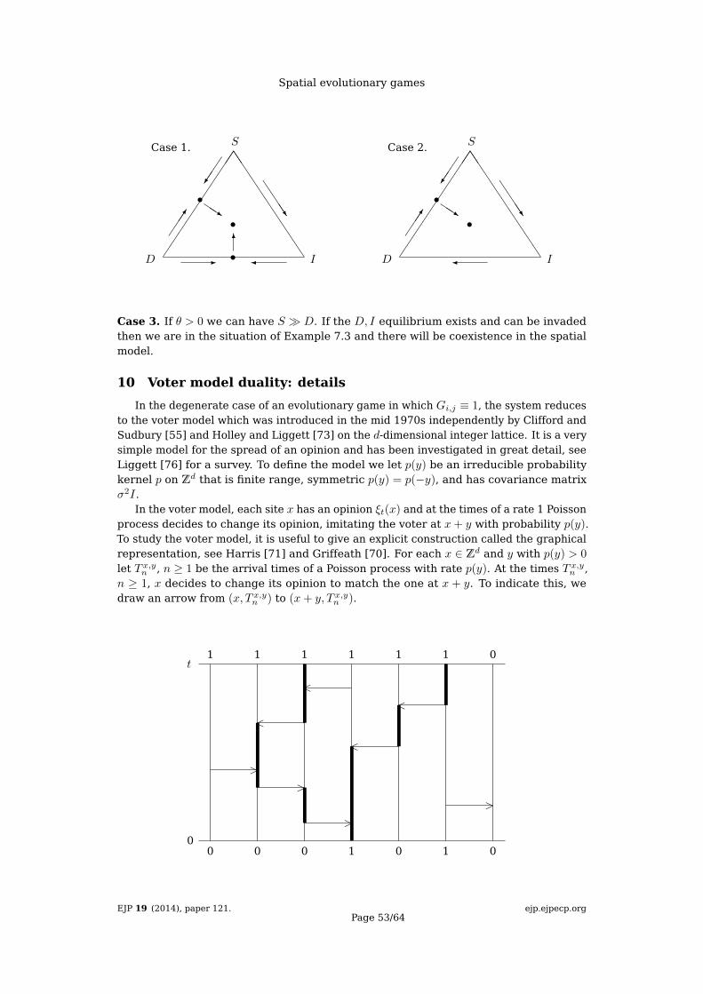
Spatial evolutionary games
Case 1.
JJJJJJJJJJ
S
D I
•
•
•QQs
6
JJJJ
-
Case 2.
JJJJJJJJJJ
S
D I
•
•QQs
JJJJ
Case 3. If θ > 0 we can have S D. If the D, I equilibrium exists and can be invadedthen we are in the situation of Example 7.3 and there will be coexistence in the spatialmodel.
10 Voter model duality: details
In the degenerate case of an evolutionary game in which Gi,j ≡ 1, the system reducesto the voter model which was introduced in the mid 1970s independently by Clifford andSudbury [55] and Holley and Liggett [73] on the d-dimensional integer lattice. It is a verysimple model for the spread of an opinion and has been investigated in great detail, seeLiggett [76] for a survey. To define the model we let p(y) be an irreducible probabilitykernel p on Zd that is finite range, symmetric p(y) = p(−y), and has covariance matrixσ2I.
In the voter model, each site x has an opinion ξt(x) and at the times of a rate 1 Poissonprocess decides to change its opinion, imitating the voter at x+ y with probability p(y).To study the voter model, it is useful to give an explicit construction called the graphicalrepresentation, see Harris [71] and Griffeath [70]. For each x ∈ Zd and y with p(y) > 0
let T x,yn , n ≥ 1 be the arrival times of a Poisson process with rate p(y). At the times T x,yn ,n ≥ 1, x decides to change its opinion to match the one at x + y. To indicate this, wedraw an arrow from (x, T x,yn ) to (x+ y, T x,yn ).
0 0 0 1 0 1 0
1 1 1 1 1 1 0
0
t
<
<
<
<
>
>
>
>
EJP 19 (2014), paper 121.Page 53/64
ejp.ejpecp.org

Spatial evolutionary games
To define the dual process ζx,ts , which we think of as the motion of a particle, we startwith ζx,t0 = x. To define the dynamics we start at x at time t and work down the graphicalrepresentation. The process stays at x until the first time t − r that it encounters thetail of an arrow x. At this time, the particle jumps to the site x + y at the head of thearrow, i.e., ζx,tr = x+ y. The particle stays at x+ y until the next time the tail of an arrowis encountered and then jumps to the head of the arrow etc. The definition of the dualguarantees that if ξt(x) is the opinion of x at time t in the voter model then we have theresult called (4.1) in the introduction
ξt(x) = ξt−s(ζx,ts )
For fixed x and t, ζx,ts is a random walk that jumps at rate 1 and by an amount withdistribution p(y). It should be clear from the definition that if ζx,ts = ζy,ts for some s thenthe two random walks will stay together at later times. For these reasons the ζx,ts arecalled coalescing random walks.
Having a dual random walk starting from x for each t is useful for the derivationof (4.1). However for some computations it is more convenient to have a single setvalued dual process ζBt that starts with a particle at each point of B, particles move asindependent random walks until they hit, at which time they coalesce to 1. Extendingthe reasoning that lead to (4.1)
P (ξt(x) = 1 for all x ∈ B) = P (ξ0(y) = 1 for all y ∈ ζBt ) (10.1)
Holley and Liggett (1975) have shown
Theorem 10.1. In d ≤ 2 the voter model approaches complete consensus, i.e., P (ξt(x) =
ξt(y)) → 1. In d ≥ 3 if we start from product measure with density u (i.e., we assignopinions 1 and 0 independently to sites with probabilities u and 1− u) then as t→∞, ξutconverges in distribution to ξu∞, a stationary distribution, νu, in which a fraction u of thesites have opinion 1.
Proof. We will give the proof here since it is short and we think it will be instructive forreaders not familiar with duality. Our assumptions imply that p(y) has mean 0 and finitevariance. Well known results for random walk imply that in d ≤ 2 the associated randomwalk is recurrent. This implies that two independent random walks will eventually meetand hence the probability of disagreement between two sites in the voter model
P (ξt(x) 6= ξt(y)) ≤ P (ζx,tt 6= ζy,tt )→ 0
To prove the second result it suffices to show that ξut converges in distribution to a limitξu∞, for then standard results for Markov processes will imply that the distribution of ξu∞is stationary. To do this, we use (10.1) to conclude
P (ξut (x) = 1 for all x ∈ B) = E(u|ζ
Bt |)
t → |ζBt | is decreasing, and u|ζBt | ≤ 1, so P (ξt(x) = 1 for all x ∈ B) converges to a limit
φ(B) for all finite sets B. Since the probabilities φ(B) determine the distribution of ξu∞,the proof is complete.
11 Proofs of the coalescence identities
Let v1, v2, v3 be independent and have distribution p. In this section we prove thecoalescence identities stated in Section 4
Lemma 11.1. p(0|v1 + v2) = p(0|v1) = p(v1|v2)
EJP 19 (2014), paper 121.Page 54/64
ejp.ejpecp.org

Spatial evolutionary games
Proof. Let Sn be the discrete time random walk with jumps distributed according to pand let
h(x) = Px(Sn 6= 0 for all n ≥ 0)
be the probability the walk never returns to 0 starting from x. By considering whathappens on the first step h(v1) = h(v1 + v2). Since v1 and −v1 have the same distributionh(v1 + v2) = h(v2 − v1). The two results follow since p(x|y) = h(y − x).
Lemma 11.2. p(v1|v2 + v3) = (1 + 1/κ)p(0|v1)
Proof. Starting at S0 = −v1, S1 = v2−v1 and S2 = v2 +v3−v1. Since P−v1(S1 = 0) = 1/κ.
h(v2 + v3 − v1)− h(v1) = P−v1(S1 = 0, Sn 6= 0 for n ≥ 2)
= (1/κ)P0(Sn 6= 0 for n ≥ 1) = (1/κ)h(v3) = (1/κ)p(0|v1)
which proves the desired result
From the two particle identities we easily get some for three particles. The startingpoint is to note that considering the possibilities for y when x and z don’t coalesce wehave a result we earlier called (4.4)
p(x|z) = p(x|y|z) + p(x, y|z) + p(x|y, z)
Combining this identity with one for another pair that shares a site in common leads toidentities that relate the three ways three particles can coalesce to give two.
Lemma 11.3. p(0, v1|v1 + v2) = p(0, v1 + v2|v1) = p(v1, v1 + v2|0) and hence
p(0|v1) = 2p(x, y|z) + p(0|v1|v1 + v2)
where x, y, z is any ordering of 0, v1, v1 + v2.
Proof. Using (4.4)
p(0|v1) = p(0|v1|v1 + v2) + p(v1, v1 + v2|0) + p(0, v1 + v2|v1)
p(0|v1 + v2) = p(0|v1|v1 + v2) + p(v1, v1 + v2|0) + p(0, v1|v1 + v2)
p(v1|v1 + v2) = p(0|v1|v1 + v2) + p(0, v1 + v2|v1) + p(0, v1|v1 + v2)
Since p(0|v1 + v2) = p(0|v1) by Lemma 4.2 the first result follows. Translation invarianceimplies p(0|v1) = p(0|v2) = p(v1|v1 + v2) so comparing the first and third lines gives thesecond result. The displayed identity follows from the first two and first and third in theproof.
Lemma 11.4. p(v1, v2|v2 + v3) = p(v2, v2 + v3|v1) = p(v1, v2 + v3|v2) + (1/κ)p(0|v1) andhence
p(v1|v2)(1 + 1/κ) = 2p(v2, v2 + v3|v1) + p(v1|v2|v2 + v3)
= 2p(v1, v2|v2 + v3) + p(v1|v2|v2 + v3)
p(v1|v2)(1− 1/κ) = 2p(v1, v2 + v3|v2) + p(v1|v2|v2 + v3)
Proof. Using (4.4)
p(v1|v2) = p(v1|v2|v2 + v3) + p(v1, v2 + v3|v2) + p(v2, v2 + v3|v1)
p(v2|v2 + v3) = p(v1|v2|v2 + v3) + p(v1, v2 + v3|v2) + p(v1, v2|v2 + v3)
p(v1|v2 + v3) = p(v1|v2|v2 + v3) + p(v2, v2 + v3|v1) + p(v1, v2|v2 + v3)
EJP 19 (2014), paper 121.Page 55/64
ejp.ejpecp.org

Spatial evolutionary games
Since p(v2|v2 + v3) = p(v1|v2) by Lemma 11.1, the first result follows. Noting that Lemma11.2 implies p(v1|v2 + v3) = p(0|v1)(1 + 1/κ) and subtracting the second equation in theproof from the third gives
(1/κ)p(0|v1) = p(v2, v2 + v3|v1)− p(v1, v2 + v3|v2)
and the second result follows. To get the first displayed equation in the lemma, substitutep(v1, v2 + v3|v2) = p(v2, v2 + v3|v1)− (1/κ)p(0|v1) in the first equation in the proof. Sincep(v1, v2|v2 + v3) = p(v2, v2 + v3|v1) the second follows. For the third one, use p(v2, v2 +
v3|v1) = p(v1, v2 + v3|v2) + (1/κ)p(0|v1) in the first equation in the proof.
12 Derivation of the limiting PDE
In this section we will compute the functions φiB(u) and φiD(u) that appear in thelimiting PDE. To do this it is useful to note that since
∑j ui = 1 we can write the
replicator equation (5.1) as
duidt
=∑j 6=i
∑k
uiujuk(Gi,k −Gj,k) (12.1)
where the restriction to j 6= i comes from noting that the when i = j the G’s cancel.
12.1 Birth-Death dynamics
By (3.4) the perturbation is
hi,j(0, ξ) =∑k
f(2)j,k (0, ξ)Gj,k
where f (2) was defined in Section 3.1. In the multi-strategy case the rate of change ofthe frequency of strategy i in the voter model equilibrium is
φiB(u) =
⟨∑j 6=i
−1(ξ(0) = i)hi,j(0, ξ) + 1(ξ(0) = j)hj,i(0, ξ)
⟩u
=∑j 6=i
∑k
−q(i, j, k)Gj,k + q(j, i, k)Gi,k (12.2)
where q(a, b, c) = P (ξ(0) = a, ξ(v1) = b, ξ(v1 + v2) = c) and v1, v2 are independent randomchoices from N . If a 6= b then
q(a, b, c) = p(0|v1|v1 + v2)uaubuc (12.3)
+ 1(c=a)p(0, v1 + v2|v1)uaub + 1(c=b)p(0|v1, v1 + v2)uaub
Combining the last two equations, and comparing with (12.1) we see that
φiB(u) = φiR(u)p(0|v1|v1 + v2) +∑j 6=i
p(0, v1 + v2|v1)uiuj(−Gj,i +Gi,j)
+∑j 6=i
p(0|v1, v1 + v2)uiuj(−Gj,j +Gi,i)
Formula (4.5) implies that p(0, v1 + v2|v1) = p(0|v1, v1 + v2) so the last two terms can becombined into one.
φiB(u) = φiR(u)p(0|v1|v1 + v2) +∑j 6=i
p(0|v1, v1 + v2)uiuj(Gi,i −Gj,i +Gi,j −Gj,j) (12.4)
which is the formula given in (5.2)
EJP 19 (2014), paper 121.Page 56/64
ejp.ejpecp.org

Spatial evolutionary games
12.2 Death-Birth dynamics
In this case (3.6) implies that the perturbation is
hεi,j(0, ξ) = hi,j(0, ξ)− fj∑k
hi,k(0, ξ) +O(ε2)
From this we see that φiD = φiB + ψiD where
ψiD =
⟨∑j 6=i
1(ξ(0) = i)fj(0, ξ)∑k
hi,k(0, ξ)−∑j 6=i
1(ξ(0) = j)fi(0, ξ)∑k
hj,k(0, ξ)
⟩u
.
Let v1, v2 and v3 be independent random picks from N and let
q(a, b, c, d) = P (ξ(v1) = a, ξ(0) = b, ξ(v2) = c, ξ(v2 + v3) = d)
we can write the new term in φiD as
ψiD =∑j 6=i
∑k,`
[q(j, i, k, `)− q(i, j, k, `)]Gk,` (12.5)
Adding and subtracting q(i, i, k, `) we can do the sum over j to get
ψiD =∑k,`
[q(i, k, `)− q(i, ·, k, `)]Gk,` (12.6)
where q(a, b, c) is as defined above and
q(a, ·, b, c) = P (ξ(v1) = a, ξ(v2) = b, ξ(v2 + v3) = c)
If we let q(b, c) = P (ξ(v2) = b, ξ(v2 + v3) = c) and write the sum in (12.6) as∑k 6=i∑` plus∑
`
[q(i, i, `)− q(i, ·, i, `)]G(i, `) = [q(i, `)− q(i, `)]Gi,`
+∑k 6=i
∑`
[−q(k, i, `) + q(k, ·, i, `)]Gi,`
To see this move the second sum on the right to the left.Putting things together we have
ψiD =∑k 6=i
∑`
[q(i, k, `)− q(i, ·, k, `)]Gk,` +∑k 6=i
∑`
[−q(k, i, `) + q(k, ·, i, `)]Gk,`
One half of the sum is ∑k,`
q(i, k, `)Gk,` − q(i, k, `)Gk,` = −φiB
Since φiD = φiB + ψiD we have
φiD =∑k,`
−q(i, ·, k, `)G(k, `) + q(i, ·, k, `)Gk,` (12.7)
Note the similarity to (12.2). If a 6= b then
q(a, ·, b, c) = p(v1|v2|v2 + v3)uaubuc (12.8)
+ 1(c=a)p(v1, v2 + v3|v2)uaub + 1(c=b)p(v1|v2, v2 + v3)uaub
EJP 19 (2014), paper 121.Page 57/64
ejp.ejpecp.org

Spatial evolutionary games
As in the Birth-Death case it follows that
φiD(u) = φiR(u)p(v1|v2|v2 + v3) +∑j 6=i
p(v1, v2 + v3|v2)uiuj(−Gj,i +Gi,j)
+∑j 6=i
p(v1|v2, v2 + v3)uiuj(−Gj,j +Gi,i)
By (4.6) p(v1, v2 + v3|v2) = p(v1|v2, v2 + v3)− (1/κ)p(v1|v2), so we can rewrite this as
φiD(u) = φiR(u)p(v1|v2|v2 + v3) +∑j 6=i
p(v1|v2, v2 + v3)uiuj(Gi,i −Gj,i +Gi,j −Gj,j)
− (1/κ)p(v1|v2)∑j 6=i
uiuj(−Gj,i +Gi,j) (12.9)
13 Two strategy games with Death-Birth updating
13.1 Computation of the phase diagram given in Figure 3
We give the details behind the conclusions drawn in Figure 2. In the Death-Birth case
θ =p2p1
(R+ S − T + P )− p(v1|v2)
κp1(S − T )
To find the boundaries between the four cases using (6.5), we let µ = p2/p1 ∈ (0, 1) andν = p(v1|v2)/κp1. We have α = γ when
R− T = −θ = −µ(R+ S − T − P ) + ν(S − T )
= −(µ− ν)(R+ S − T − P )− ν(R− P )
Clearly ν > 0. The fact that µ− ν > 0 follows from (4.13). Rearranging gives
(µ− ν)(S − P ) + ν(R− P ) = (1 + µ− ν)(T −R)
and hence
T −R =µ− ν
1 + µ− ν(S − P ) +
ν
1 + µ− ν(R− P ) (13.1)
Repeating the last calculation shows that β = δ when
S − P = −θ = −(µ− ν)(R+ S − T − P )− ν(R− P ) < 0
Rearranging gives (1 + µ− ν)(S − P ) + ν(R− P ) = (µ− ν)(T −R), and we have
T −R =1 + µ− νµ− ν
(S − P ) +ν
µ− ν(R− P ) (13.2)
To find the intersections of the lines in (13.1) and (13.2), we set
µ− ν1 + µ− ν
(S − P ) +ν
1 + µ− ν(R− P ) =
1 + µ− νµ− ν
(S − P ) +ν
µ− ν(R− P )
which holds if
(µ− ν)2(S − P ) + ν(µ− ν)(R− P ) = (1 + µ− ν)2(S − P ) + ν(1 + µ− ν)(R− P )
Solving gives
S − P =−ν(R− P )
1 + 2(µ− ν)< 0
EJP 19 (2014), paper 121.Page 58/64
ejp.ejpecp.org

Spatial evolutionary games
Using (13.2) we see that at this value of S
T −R = −ν(R− P )
µ− ν
[1 + µ− ν
1 + 2(µ− ν)− 1
]=
ν(R− P )
1 + 2(µ− ν)> 0
To simplify the formulas for (13.1) and (13.2) let
P ∗ = P − ν(R− P )
1 + 2(µ− ν)R∗ = R+
ν(R− P )
1 + 2(µ− ν)(13.3)
From this and (13.1) we see that
T −R∗ = T −R− ν(R− P )
1 + 2(µ− ν)
=µ− ν
1 + µ− ν(S − P ) +
ν
1 + µ− ν(R− P )− ν(R− P )
1 + 2(µ− ν)
=µ− ν
1 + µ− ν(S − P )− µ− ν
1 + µ− ν· ν(R− P )
1 + 2(µ− ν)=
µ− ν1 + µ− ν
(S − P ∗)
A similar calculation using (13.2) shows that
T −R∗ = T −R− ν(R− P )
1 + 2(µ− ν)
=1 + µ− νµ− ν
(S − P ) +ν
µ− ν(R− P )− ν(R− P )
1 + 2(µ− ν)
=1 + µ− νµ− ν
(S − P ) +1 + µ− νµ− ν
· ν(R− P )
1 + 2(µ− ν)=
1 + µ− νµ− ν
(S − P ∗)
so the two lines can be written as
T −R∗ =µ− ν
1 + µ− ν(S − P ∗) T −R∗ =
1 + µ− νµ− ν
(S − P ∗)
This leads to the four regions drawn in Figure 2. In the lower left region where there isbistability, 1’s win if u > 1/2 or what is the same if strategy 1 is better than strategy 2when u = 1/2 or
R+ S − T − P > −2θ
Plugging in the value of θ this becomes
(1 + 2(µ− ν))(R+ S − T − P ) > −2ν(R− P ) (13.4)
Dividing each side by 1+2(µ−ν) and recalling (13.3) this can be written asR∗−T > P ∗−S.For the proof of Theorem 6.2 it is useful to write this as
1 + 2µ
1 + 2(µ− ν)R+ S > T +
1 + 2µ
1 + 2(µ− ν)(13.5)
In the coexistence region, the equilibrium is
u =S − P + θ
S − P + T −R(13.6)
Plugging in the value of θ, we see that u is constant on lines through (S, T ) = (R∗, P ∗).Again for the proof of Theorem 6.2 a less compact form is more desirable. Recalling thedefinition of θ we see that u > 1/2 when
2(S − P ) + 2µ(R+ S − T − P )− 2ν(S − T ) > S − P + T −R
EJP 19 (2014), paper 121.Page 59/64
ejp.ejpecp.org

Spatial evolutionary games
which rearranges to become
(1 + 2µ)R+ [1 + 2(µ− ν)]S > [1 + 2(µ− ν)]T + (1 + 2µ)P
Dividing by 1 + 2(µ− ν) this becomes (13.5). To prove Theorem 6.2 now, we note that
1 + 2µ =p1 + 2p2
p1= (1 + 1/κ)
p(v1|v2)
p1
1 + 2(µ− ν) = (1 + 1/κ)p(v1|v2)
p1− 2
p(v1|v2)
κp1
so we have1 + 2µ
1 + 2(µ− ν)=κ+ 1
κ− 1
13.2 Proof of Tarnita’s formula
Lemma 13.1. Suppose the φ in the limiting PDE is cubic. The limiting frequency of 1’sin the PDE is > 1/2 (and hence also in the particle system with small ε) if and only ifφ(1/2) > 0.
Proof. As explained in the proof of Theorem 6.1 given in [56] the behavior of the PDE isrelated to the shape of φ in the following way.
φ′(0) > 0, φ′(1) > 0. There is an interior fixed point u, which is the limiting frequency. Ifφ(1/2) > 0 then u > 1/2.
φ′(0) > 0, φ′(1) < 0. φ > 0 on (0, 1) so the system converges to 1.
φ′(0) < 0, φ′(1) > 0. φ < 0 on (0, 1) so the system converges to 0.
φ′(0) < 0, φ′(1) < 0. There is an unstable fixed point u. If u < 1/2 which in this case isequivalent to φ(1/2) > 0 the system converges to 1, otherwise it converges to 0.
Combining our observations proves the desired result.
Death-Birth updating. In this case, we have φ(1/2) > 0 if
a+ b+ θ > c+ d− θ
where θ = (p2/p1)(a+b−c−d)−p(v1|v2)/κp1. Rearranging we see that the last inequalityholds if
κ(p1 + 2p2)(a+ b− c− d)− 2p(v1|v2)(b− c)
Using (4.9) p1 + 2p2 = p(v1|v2)(1 + 1/κ) this becomes
p(v1|v2)[(κ+ 1)(a− d) + (κ− 1)(b− c)
which is the condition in Tarnita’s formula with σ = (κ+ 1)/(κ− 1).
14 Equilibria for three strategy games
Recall that we can write the game matrix as 0 α3 β2β3 0 α1
α2 β1 0
EJP 19 (2014), paper 121.
Page 60/64ejp.ejpecp.org

Spatial evolutionary games
In equilibrium all three strategies must have the same payoff so an interior equilibrium(x, y, 1− x− y) must satisfy
α3y + β2(1− x− y) = β3x+ α1(1− x− y) = α2x+ β1y
Equating the first to the third, the second to the third and rearranging we obtain
(α2 + β2)x+ (β1 + β2 − α3)y = β2
(α1 + α2 − β3)x+ (α1 + β1)y = α1
From this we see that [to find x look at (α1 + β1)E1 − (β1 − β2 − α3)E2]
x =β2(α1 + β1)− α1(β1 + β2 − α3)
(α1 + β1)(α2 + β2)− (α1 + α2 − β3)(β1 + β2 − α3)
y =α1(α2 + β2)− β2(α1 + α2 − β3)−
(α1 + β1)(α2 + β2)− (α1 + α2 − β3)(β1 + β2 − α3)
The 13 terms in the denominator reduce to nine:
D = α1α2 + α1α3 + α2α3 + β1β2 + β1β3 + β2β3 − α1β1 − α2β2 − α3β3
The numerators for x and y reduce to 3 terms each, so the equilibrium must be:
u1 =α1α3 + β1β2 − α1β1
D
u2 =α2α1 + β2β3 − α2β2
D
u3 =α3α2 + β3β1 − α3β3
D.
which is the formula given in (7.2).
References
[1] von Neumann, J., and Morgenstern, O. (1944) The Theory of Games and Economic Behavior.Princeton U. Press MR-0011937
[2] Maynard Smith, J., and Price, G.R. (1973) The logic of animal conflict. Nature. 401, 268–371
[3] Maynard Smith, J. (1982) Evolution and the Theory of Games. Cambridge U. Press
[4] Axelrod, R., and Hamilton, W.D. (1981) The evolution of cooperation. Science. 211, 1390–1396MR-0686747
[5] Axelrod, R. (1984) The Evolution of Cooperation. Basic Books, New York
[6] Harsanyi, J., and Selten, R. (1988) General Theory of Equilibrium in Games. MIT Press,Cambridge MA MR-0956053
[7] Hofbauer, J., and Sigmund, K. (1998) Evolutionary Games and Population Dynamics. Cam-bridge U. Press MR-1635735
[8] Hofbauer, J., and Sigmund, K. (2003) Evolutionary game dynamics. Bull. Amer. Math. Soc. 40,479–519 MR-1997349
[9] Nowak, M.A., and Sigmund, K. (2004) Evolutionary dynamics of biological games. Science.303, 793–799
[10] Nowak, M.A. (2006) Evolutionary Dynamics. Belknap Press, Harvard University. Spatial
games MR-2252879
[11] Nowak, M.A., and May, R.M. (1992) Evolutionary games and spatial chaos. Nature. 359,826–829
[12] Nowak, M.A., and May, R.M. (1993) The spatial dilemmas of evolution. Int. J. Bifurcat. Chaos.3, 35–78 MR-1218718
EJP 19 (2014), paper 121.Page 61/64
ejp.ejpecp.org

Spatial evolutionary games
[13] Huberman, B., and Glance, N. (1993) Evolutionary games and computer simulation. Proc.Natl. Acad. Sci., IUSA. 90, 7716–7718
[14] Nowak, M.A., Bonhoeffer, S., and and May, R.M. (1994) More spatial games. Int. J. Bifurcat.Chaos. 4, 33–56 MR-1276803
[15] Nowak, M.A., Bonhoeffer, S., and and May, R.M. (1994) Spatial games and the maintenanceof cooperation. Proc. Natl. Acad. Sci. USA. 91, 4877–4881
[16] Durrett, R., and Levin, S. (1994) The importance of being discrete (and spatial). Theor. Pop.Biol. 46, 363–394
[17] Killingback, T., and Doebli, M. (1996) Spatial evolutionary game theory: Hawks and Dovesrevisited. Proc. Roy. Soc. London, B. 263, 1135–1144
[18] Killingback, T., and Doebli, M. (1998) Self-oraganized criticality in spatial evolutionary gametheory. J. Theoretical Biology. 191, 335–340
[19] Szabó, G., and Töke, C. (1998) Evolutionary prisoner’s dliemma game on a square lattice.Phys. Rev., E. 58, 69–73
[20] van Baalen, M., and Rand, D.A. (1998) The unit of selection in viscous populations and theevolution of altruism. J. Theor. Biol. 193, 631-648
[21] Hauert, C. (2001) Fundamental clusters in spatial 2× 2 games. Proc. Roy. Soc. London, B.268, 761–769
[22] Hauert, C. (2002) Effects of space on 2× 2 games. International Journal of Biifurcation andChaos. 12, 1531–1548 MR-1924058
[23] Hauert, C., and Doebeli, M. (2004) Spatial structure often inhibits the evolution of cooperationin the snowdrift game. Nature. 428, 643–646
[24] Hauert, C., and Szabó, G. (2005) Game theory and physics. Am. J. Physics. 73, 405-414MR-2147955
[25] Szabo, G., Vukov, J., and Szolnoki, A. (2005) Phase diagrams for an evolutionary Prisoner’sdilemma game on two-deimnsional lattices. Phys. Rev. E. 72, paper 047107
[26] Doebeli, M., and Hauert, C. (2005) Models of cooperation based on the Prisoner’s Dilemmaand the Snowdrift game. Ecology Letters. 8, 748–766
[27] Lieberman, E., Hauert, C., and Nowak, M.A. (2005) Evolutionary dyanmics on graphs. Nature.433, 312–316
[28] Ohtsuki, H., and Nowak, M.A. (2006) Evolutionary games on graphs. J. Theoretical Biology.243, 86–97 MR-2279323
[29] Ohtsuki, H., Hauert, C., Lieberman, E., and Nowak, M.A. (2006) A simple rule for theevolution of cooperation on graphs and social networks. Nature. 441, 502–505
[30] Ohtsuki, H., and Nowak, M.A. (2006) The replicator equation on graphs. J. Theor. Biol. 243,86–97 MR-2279323
[31] Szabó, G., and Fáth, G. (2007) Evolutionary games on graphs. Physics Reports. 46, 97–216MR-2332485
[32] Gore, J., Youk, H., and van Oudenaarden, A. (2009) Snowdrift game dynamics and facultativecheating in yeast. Nature. 459, 253–256.
[33] Roca, C.P., Cuesta, J.A., and Sanchez, A. (2009) Effect of spatial structure on the evolution ofcooperation. Phys. Rev. E. 80, paper 046106
[34] Roca, C.P., Cuesta, J.A., and Sanchez, A. (2009) Evolutionary game theory: temporal andspatial effects beyond replicator dynamics. Phys. Life Rev. 6, 208–249
[35] Tarnita, C.E., Ohtsuki, H., Antal, T., Feng, F., and Nowak, M.A. (2009) Strategy selection instructured populations. J. Theoretical Biology 259, 570–581 MR-2973175
[36] Tarnita, C.E., Wage, N., and Nowak, M. (2011) Multiple strategies in structured populations.Proc. Natl. Acad. Sci. 108, 2334–2337
[37] Lanchier, N. (2014) Evolutionary games on the lattice: payoffs affecting birth and death rates.Ann. Apppl. Probab., to appear
[38] Evilsizor, S., and Lanchier, N. (2013) Evolutionary games on the lattice: Best-responsedynamics. arXiv:1310.5192 Evolutionary games modeling cancer MR-3256875
EJP 19 (2014), paper 121.Page 62/64
ejp.ejpecp.org

Spatial evolutionary games
[39] Axelrod, R., Axelrod, D.E., and Pienta, K.J. (2006) Evolution of cooperation among tumor cells.Proc. Natl. Acad. Sci. 103, 13474–13479
[40] Basanta, D., and Deutsch, A. (2008) A game theoretical perspective on the somatic evolutionof cancer. Chapter 5 in Selected Topics in Cancer Modeling. edited by N. Bellomo. Spring,New York
[41] Basanta, D., Gatenby, R.A., and Anderson, A.R.A. (2012) Exploiting evolution to treat drugresistance: Combination therapy and the double bind. Molecular Pharmaceutics. 9, 914–921
[42] Basanta, D., Hatzikirou, H., and Deutsch, A. (2008) Studying the invasiveness in tumoursusing game theory. The European Physical Journal B 63, 393–397 MR-2421563
[43] Basanta, D., Scott, J.G., Rockne, R., Swanson, K.R., and Anderson, A.R.A. (2011) The role ofIDH1 mutated tumor cells in secondary glioblastomas: an evolutionary game theoretic view.Physical Biology. 8, paper 015016
[44] Basanta, D., Scott, J.G., Fishman, M.N., Ayala, G., Hayward, S.W., and Anderson, A.R.A. (2012)Investigating prostate cancer tumor-stroma interactions: clinical and biological insights froman evolutionary game. British J. Cancer. 106, 174–181
[45] Basanta, D., Simon, M., Hatzikirou, H., and Deutsch, A. (2008) Evolutionary game theoryelucidates the role of glycolysis in glioma progression and invasion. Cell Proliferation. 41,980–987
[46] Dingli, D., Chalub, F.A.C.C., Santos, F.C., van Segbroeck, S., and Pahceco, J.M. (2009) Cancerphenotype as the outcome of an evolutionary game between normal and malignant cells.British J. Cancer. 101, 1130–1136
[47] Swierniak, A., and Krzeslak, M. (2013) Application of evolutionary games to modelingcarcinogenesis. Math. Biosciences and Engineering. 10, 873–911 MR-3046270
[48] Tomlinson, I.P.M. (1997) Game-theory models of interactions between tumor cells. EuropeanJ. Cancer. 33, 1495–1500
[49] Tomlinson, I.P.M., and Bodmer. W.F. (1997) Modelling the consequences of interactionsbetween tumor cells. British J. Cancer. 78, 157–160
Other references
[50] Aronson, D.G. and Weinberger, H.F. (1975) Nonlinear diffusion in population genetics, com-bustion, and nerve pulse propagation. Pages 5–49 in Partial Differential Equations andRelated Topics. Springer Lecture Notes in Math 446, Springer, New York. MR-0427837
[51] Aronson, D.G. and Weinberger, J.F. (1978) Multidimensional nonlinear diffusion arising inpopulation genetics. Adv. in Math. 30, 33–76. MR-0511740
[52] Blume, L.E. (1993) The statistical mechanics of strategic interaction. Games and EconomicBehavior. 5, 387-424 MR-1227917
[53] Bomze, I.M. (1983) Lotka-Volterra equation and replicator dynamics. Biological Cybernetics.48, 201–211
[54] Bomze, I.M. (1983) Lotka-Volterra equation and replicator dynamics: new issues in theclassification. Biological Cybernetics. 72, 447–453
[55] Clifford, P. and Sudbury, A. (1973) A model for spatial conflict. Biometrika. 60, 581–588MR-0343950
[56] Cox, T., Durrett, R., and Perkins, E. (2011) Voter model perturbations and reaction diffusionequations. Astérisque, to appear. arXiv:1103.1676 MR-3075759
[57] Durrett, R. (1992) Predator-prey systems. Pages 37-58 in Asymptotic problems in probabilitytheory: stochastic models and diffusions on fractals. (1992) Edited by K.D. Elworthy and N.Ikeda. Pitman Research Notes 283. Longman, Essex, England MR-1354150
[58] Durrett, R. (1995) Ten Lectures on Particle Systems. Page 97–198 in Springer Lecture Notesin Math 1608 MR-1383122
[59] Durrett, R. (2002) Mutual invadability implies coexistence in spatial models. Memoirs of theAMS. Volume 156, Number 740 MR-1879853
[60] Durrett, R. (2009) Coexistence in Stochastic Spatial Models. Ann. Appl. Prob. 19, 477–496MR-2521876
EJP 19 (2014), paper 121.Page 63/64
ejp.ejpecp.org

Spatial evolutionary games
[61] Durrett, R. (2010) Probability: Theory and Examples. 4th Edition. Cambridge U. PressMR-2722836
[62] Durrett, R., and Levin, S. (1997) Allelopathy in spatially distributed populations. J. Theor.Biol. 185, 165–172
[63] Durrett, R., and Neuhauser, C. (1994) Particle systems and reaction diffusion equations. Ann.Prob. 22 (1994), 289–333 MR-1258879
[64] Durrett, R., and Swindle, G. (1994) Coexistence results for catalysts. Prob. Th. Rel. Fields, 98(1994), 489–515 MR-1271107
[65] Ellison, G. (1993) Learning, local interaction, and coordination. Econometrica. 61, 1047–1071MR-1234793
[66] Fife, P.C. and McLeod, J.B. (1977) The approach of solutions of nonlinear diffusion equationsto traveling front solutions. Arch. Rat. mech. Anal. 65, 335–361 MR-0442480
[67] Fife, P.C. and McLeod, J.B. (1981) A phase plane discussion of convergence to traveling frontsfor nonlinear diffusion. Arch. Rat. mech. Anal. 75, 281–314 MR-0607901
[68] Goh, B.S. (1976) Global stability in two species interactions. Journal of Mathematical Biology.3, 313–318 MR-0418958
[69] Gore, J., Youk, H., and van Oudenaarden, A. (2009) Snowdrift game dynamics and facultativecheating in yeast. Nature. 459, 253–256
[70] Griffeath, D.S. (1978) Additive and Cancellative Interacting Particle Systems. SpringerLecture Notes in Math. MR-0538077
[71] Harris, T.E. (1976) On a class of set-valued Markov processes. Ann. Prob. 4, 175–194 MR-0400468
[72] Harrison, G.W. (1977) Global stability of food chains. American Naturalist. ?, 455–457
[73] Holley, R., and Liggett, T. (1975) Ergodic theorems for weakly interacting systems and thevoter model. Ann. Probab. 4, 195–228 MR-0402985
[74] Kandori, M., Mailath, G., and Rob, R. (1993) Learning, mutation, and long run equilibria.Econometrica. 61, 29–56 MR-1201702
[75] Licht, A.M. (1999) Games commissions play" 2×2 games of international securities regulation.Yale Journal of International Law. 24, 61–128
[76] Liggett, T.M. (1999) Stochastic Interacting Systems: Contact, Voter and Exclusion Processes.Springer, New York. MR-1717346
Acknowledgments. We thank Ed Perkins and a second anonymous referee for sugges-tions that improved the correctness and readability of the paper.
EJP 19 (2014), paper 121.Page 64/64
ejp.ejpecp.org


![Finding Significant Fourier Coefficients: Clarifications, … · 2018. 12. 14. · arXiv:1607.01842v4 [cs.CR] 13 Dec 2018 Finding Significant Fourier Coefficients: Clarifications,](https://img.pdfslide.us/doc/110x75/5fe0b1a1b161d147ba753552/finding-signiicant-fourier-coeficients-clariications-2018-12-14-arxiv160701842v4.jpg)


![An Introduction to Scaling, Spatial and Evolutionary ... Introduction to Scaling, Spatial and Evolutionary Modelling in Ecology ... [Table[m[i,j],{i,1,50},](https://img.pdfslide.us/doc/110x75/5ac67b8d7f8b9a5c558df968/an-introduction-to-scaling-spatial-and-evolutionary-introduction-to-scaling.jpg)