Embed Size (px)
Citation preview

Spatial-Difference-in-Differences (SIDD) Models for Impact of New Mass Rapid Transit
Line on Private Housing Values
Mi DIAO1, Delon LEONARD2, and Tien Foo SING3
Date: 23 May 2017
Abstract:
This study uses the opening of the new Circle Line (CCL) in Singapore as a natural experiment to
test the effects of urban rail transit networks on non-landed private housing values. We use a
network distance measure and a local-polynomial-regression approach to identify the CCL impact
zone that shows discontinuity in housing price gradient between a treatment zone and a control
zone. We then estimate a spatial difference-in-differences model that accounts for spatial
autocorrelation in housing price changes in the two zones “before and after” the opening of the
CCL, in addition to other controls, such as housing attributes, local amenities, spatial and temporal
fixed effects. We find that the opening of the CCL increase housing value in the treated
neighbourhoods located within the 600-metre network distance from the new CCL stations by
approximately 7.8%, relative to other properties in the untreated neighbourhoods. We also find
significant “anticipation” effects that appear 1 year prior to the opening of the CCL line, and the
effects diminish closer to the actual opening date. The results imply that inter-dependence spatial
structure between the treated and the untreated neighbourhoods is relevant and significant, if
neglected, may lead to over-estimation of capitalization effects of new transit lines on housing
values.
Keyword: Urban rail transit network; housing values; network distance; local polynomial
regression; spatial difference-in-differences estimator; spatial autocorrelation
JEL Code: C21, R4, R21,
1 Department of Real Estate, National University of Singapore. Email: [email protected]
2 Department of Real Estate, National University of Singapore. Email: [email protected]
3 Corresponding author. Department of Real Estate/ Institute of Real Estate Studies (IRES), National University of
Singapore: Email: [email protected]

1
1. Introduction
An efficient and environmentally-friendly urban rail transit system (RTS) has become an
indispensable part of urban infrastructure in today’s cities. Governments of many developed and
developing countries have invested a huge sum of public money to build new and/or expand
existing urban RTSs in their major cities. New RTS lines improve connectivity and bring
agglomeration to the city centre; and as a city grows, economic externalities could spill over
through extending the RTS lines to other areas outside the city. New RTS investments help narrow
the rental gaps between the city centre and the outlying, and as a result, flatten the bid-rent gradient
(McMillen and McDonald, 2004; Zheng and Kahn, 2008).
There are other social and economic cost and benefit associated with new RTS lines. A
“substitution” effect between road and RTS transport modes is created, if some private car owners
switch to urban RTS when commuting to city centres (Baum-Snow and Kahn, 2000). When more
public road users switch to RTS, public road users could enjoy shorter travelling time on less
congested roads and reap significant reduction in marginal social costs; and in addition,
environmental quality is also improved through the reduction in greenhouse gas emissions by users
who switch from private cars and public buses to RTS.
The accessibility benefits of a RTS are local by nature. People who live near transit stations are
more likely to use the urban RTS for commuting purposes. Therefore, we expect variations in
housing prices between areas that are within and those that are outside the accessibility range of
RTS stations. Many studies have found empirical evidence of positive capitalization effects of
proximity convenience associated with new urban RTS stations on housing prices.1 However, these
studies, which usually capture capitalization effects of RTS with a distance variable (either discrete
or continuous) in the standard OLS hedonic housing price model, are vulnerable to the problems
relating to omitted variables and endogeneity in housing prices and distances to RTS stations. Some
of these problems are spatial by nature; and this paper applies three innovations in spatial statistical
tools to improve the quasi-experiment approach in capitalizing the RTS effects.
1 Evidence of positive capitalization effects of urban rail transit systems is shown in many studies across different
countries, which include studies in major US cities (non-exhaustive), such as Washington DC (Damm et al., 1980),
Atlanta (Nelson, 1992; Bowes and Ihlanfeldt, 2001), Miami (Gatzlaff and Smith, 1993), Chicago (McDonald and
Osuji, 1995; McMillen and McDonald, 2004), San Francisco (Landis et al., 1995), and other cities such as Toronto
(Bajic, 1983; Dewees, 1976), Taipei (Lin and Hwang, 2003), Seoul, (Bae et al., 2003), London (Gibbons and
Machin, 2005) and the Netherlands (Amsterdam, Rotterdam and Enschede) (Debrezione et al., 2011).

2
First, most studies use either a Euclidean distance (Baum-Snow and Kahn, 2000; Chalermpong,
2007, and others), or a Eucliean-distance-based ring buffer (Lin and Hwang, 2003; Des Rosier et
al., 2010; Dube et al, 2011; and others) to identify the treatment zone with respects to the nearest
RTS stations. At the local level, RTS stations are not usually surrounded by lands with flat and
plain topographies. Instead, they are sometimes criss-crossed by major road networks, divided by
rivers, and obstructed by other buildings. The diverse spatial and topographic features could be
potential sources of measurement errors, especially in a densely built-up urban cities. Incorrect
distance measures, if used indiscriminately without adjustments, could distort the pricing of RTS
accessibility premiums. In this study, we use a network-based distance measure to capture the
shortest route (network distance) between a house and the nearest RTS station based on the local
road network map. The network walking distance to the nearest RTS stations is a more realistic
and direct way of capturing users’ marginal willingness to pay (MWTP) in housing prices.
Second, based on social and economic considerations, central planners in most Asian high-density
cities2 are more inclined to site RTS stations in neighbourhoods with a large population coverage
to justify that the RTS services and operations are economically viable. Areas served by the RTS
stations (treatment areas) may contain both observed and unobserved demographic and spatial
attributes that are not found in those areas without the RTS convenience (control areas). While we
could include observed spatial factors, and control for unobserved spatial attributes using location
fixed effects in the model, it is difficult to separate covariance in the buyers’ demand for the local
amenities in high density areas from the effects of RTS stations. The supply inelasticity imposed
by the shortage of vacant lands near RTS stations may create, in equilibrium, disproportional price
responses to increased demand in the area. We apply the local polynomial regression (LPR), which
is a spatial innovation used in Linden and Rockoff (2008), to fit housing prices on distances to RTS
stations with a locally weighted least squares estimator. The LPR allows for non-linear
capitalization effects, which are likely to be stronger in areas near the new RTS stations where
housing supply is highly inelastic.
2 In the US cities, Bowes and Ihlanfeldt (2001) show that crime rates are higher in areas that are closer to the rail
transit stations, and housing values

3
Third, while most residents could not influence and vote on, in most instance, the decisions on the
location of a new rail transit station; they could, however, vote with their feet by moving close to
a RTS station in the neighbourhood. Families that have a high MWTP for the RTS accessibility
buy houses from families who stay near RTS stations, and yet have relatively low MWTP for the
RTS services. These new families who are unlikely to own private cars move in and displace the
existing families from the RTS neighbourhoods; they create a different form of social network for
the treatment area over time. The new RTS line attracts new local amenities and other commercial
activities into the neighbourhood. The spatial dynamics of the treatment neighbourhoods near a
new RTS line could be different from the (control) neighbourhoods not served by a RTS line. The
standard difference-in-differences (diff-in-diff) approach that assumes constant spatial attributes in
the treatment and control areas before and after the treatment could over-estimate the capitalization
effects associated with the opening of new rail transit stations. We incorporate the dynamic and
spatially-dependent treatment effects by adding spatial-autoregressive lag and error terms into our
difference-in-differences (diff-in-diff) housing price models (Anselin, 1988).
The Mass Rapid Transit (MRT) system is a rail-based transit system started running in 1987; and
it forms the backbone of the public transport system in Singapore. The MRT network has been
expanded over the years with additions of new line and stations to meet the growing commuter
demand. In this study, we use the opening of the new Circle Line (CCL), the fourth line on the
MRT network in Singapore, in a quasi-natural experiment, and apply the rigorous spatial-
dependence diff-in-diff models to evaluate the capitalization effects of the CCL on non-landed
private housing values.
Using the same LPR model as in Linden and Rockoff (2008), we identify the area within 600
meters (m) by the network distance from the closest new CCL stations as the impact (treatment)
zone. Based on the locally weighted impact zone, we sort the housing samples into a treatment
group, if the shortest network distance between houses and the closest CCL stations falls within
600m; and otherwise, into a control group. The treatment effects, which show the price premiums
for non-landed private houses in the treated zone relative to the control zone “before and after” the
opening of the new CCL, are estimated at 10.6% after controlling for housing characteristics, local
amenities, spatial and temporal fixed effects. However, when the inter-zone spatial dependence

4
structure is added to the spatial diff-in-diff (SDID) model, we find significant, but weaker treatment
effects of 7.8% for the treated houses relative to the untreated houses.
Based on the 3,755 non-landed houses in the treatment zone transacted after the opening of new
CCL stations with an aggregate value of S$4.42 billion, the treatment effects of the new CCL
opening are translated into realized economic benefits of approximately S$349.17 million. For
hosing buyers, the findings show the importance of understanding spatial variations and dynamics
when capitalizing RTS effects into housing values. For urban and transport planners, they should
be mindful of local features and land supply constraints when designing transportation policy and
value capture programs.
This paper is organized as follows. Section 2 reviews related literature in the study of the
relationships of RTS locations and housing values. Section 3 provides a brief overview of the
housing market and the MRT network in Singapore as background information. Section 4 describes
the data and empirical methodology. The Section shows graphical evidence on the impact of the
CCL using the local-polynomial-regression analysis, and discusses the identification strategy.
Section 5 presents and discusses the empirical results. Section 6 concludes the paper.
2. Literature Review
Alonso (1964), Muth (1969) and Mills (1972) argue that households trade-off between commuting
cost and housing consumptions in their residential location decisions. This premise lays down the
fundamental for the monocentric city model that predicts a negative housing price gradient with
respects to distance (transportation cost) to the employment centre. The negative price-distance
relationship, which is known as the bid rent curve in the urban economic literature, has significantly
shaped the urban landscape, and influenced spatial distributions of households and firms across a
city. Many empirical studies have shown that new urban RTS infrastructure investments could
significantly flatten the bid rent gradient, and reduce the housing price gap between urban and rural
areas (Nelson, 1992; Gatzlaff and Smith, 1993; Landis et al., 1995; McDonald and Osuji, 1995;
Bowes and Ihlanfeldt, 2001; McMillen and McDonald, 2004; and others). Increased accessibility
brought by new RTS investments is translated into housing wealth accrued to local residents via
the capitalization of the RTS line effects (Edel and Sclar 1974; Hilber and Mayer, 2009; Diao et
al., 2017).

5
A large number of empirical studies has found evidence of positive capitalization effects of
proximity to RTS stations in housing values (Gibbons and Machin 2005; Hess and Almeida, 2007;
Diao and Ferreira, 2010; Diao, 2015; among others). Debrezion et al. (2007) provide a meta-
analysis of 57 cities and suggest that property values increase by 2.3% every 250 m closer to a
railway station. There are also other studies that find insignificant, or in some cases, even negative
effect of the proximity to selected RTS stations in some cities (e.g., Gatzlaff and Smith, 1993;
Landis et al., 1995). The negative externalities are usually caused by noise and high crime rates
found in areas near RTS stations (Bowes and Ihlanfeldt, 2001, Diao et al., 2016).
Most of the early studies use a Euclidean distance measure to the closest RTS station, which is
represented either by a discrete or a continuous variable in standard hedonic models, to capture
cross-sectional variations in housing prices (For examples: Coffman and Gregson, 1998; Bowes
and Ihlanfeldt, 2001; Hess and Almeida, 2007; and Diao and Ferreira, 2010). The regional and
urban economic literature seems to fall behind in the application of GIS-based network analysis
tool in measuring distances to RTS stations. This study hopes to lead the literature in applying the
network tool to measure a distance between a house and a RTS station via the shortest route. The
network distance is a more realistic measure taking into account natural obstacles (rivers, canals,
and parks) and spatial constraint (existing buildings and rail tracks) in local areas.
The popular Rosen’s hedonic housing price models, despite having a rich set of housing and spatial
attributes, face serious endogeneity issues when applied to study the RTS effects. The models are
not able to separate unobserved factors that could influence covariance between housing price and
RTS accessibility. Some researchers use the repeated sales data to control for the endogeneity
effects between unobserved factors and urban RTS in modelling housing price changes (For
example, McMillen and McDonald; 2004; Billings; 2011; Chatman et al., 2012; Dube et al., 2013;
Kim and Lahr, 2014; Sun et al., 2015). The repeated-sales approach removes biases caused by
time-invariant omitted variables by taking the first differencing in housing prices. The basic idea
is to regress price changes on a time vector that corresponds to the time periods between
consecutive sales of the same house; and keeping the hedonic attributes of the same house and its
surrounding neighbourhood characteristics constant, price changes, if observed, must be correlated
with a new RTS line opening that falls within the repeated sale periods. By limiting the sample to

6
only houses that sell at least twice, the sample is significantly reduced; and in the sample selection
process, biases may arise because houses that are sold twice or multiple times are likely to have
different attributes from those that sell only once (Gatzlaff and Haurin, 1997).
Changes in structural characteristics and/or (dis)amenities in local areas sometimes occur over a
long period of time, and sometimes randomly; and thus differencing the repeated housing prices
alone could not adequately remove inter-temporal effects of both observed and unobserved factors.
In recent years, a quasi-experimental approach has become increasingly popular among researchers
in the regional and urban economic literature (Gibbons and Machin, 2005; Billings, 2011; Diao et
al., 2017). In a randomized experiment, sample houses are sorted into a treatment group and a
control group based on the proximity to RTS stations, and a random event, such as the opening of
new RTS stations, is used to create exogenous shocks to housing prices. The difference-in-
differences (diff-in-diff) models are estimated to test the effects on before-and-after price changes
between a treatment group (an affected area) and a control group (an unaffected area) following
the exogenous shock, controlling for observed and unobserved variations in housing and spatial
attributes. If the pre-existing between-the-group price variations change after the treatment, the
causality of new RTS stations on housing prices could be established in the local areas.
In the diff-in-diff models, defining the treatment area using proximity measures (such as linear
distance or buffer zone) is subject to omitted variable problems, especially when the selection of
the RTS station location is not exogenous. For instance, central planners are more likely to put a
RTS station in high density city centres than in sparsely populated rural areas, ceteris paribus. The
RTS effects in a densely populated city centre co-vary closely with other amenities in the areas.
Other cofounders such as shopping facilities that are attracted to areas near RTS stations could also
influence the preference of people for housing that are close to RTS stations, and it would be
difficult to measure house buyers’ MWTP for the RTS accessibility. Facing the same challenges
in the study of negative externalities of living close to convicted criminals, Linden and Rockoff
(2008) use a local polynomial regression approach to identify the treatment effects weighted by
moving-in and location of a sex offender’s house in a neighbourhood. Haninger et al. (2012) use
the same approach to study the impact of brownfield remediation; and Muehlenbachs et al. (2012)
study the impact of shale gas developments on property values. We use for the first time this spatial

7
innovation to study how the opening of new MRT line in Singapore would impact housing values
in the areas near the new MRT stations.
However, in areas undergoing dynamic changes following the opening of new RTS stations, there
is a need to control for possible auto-regressive lag and error in spatial interactions of houses within
the treatment areas, and over times (Anselin, 1988). The applications of the state-of-the-art spatial-
econometric techniques has attracted strong interests in recent years; and for examples, Chagas et
al. (2016) use the sepatial-dependence diff-in-diff (SDID) to study sugarcane production and
health; and Brasington et al. (2016) use the spatial autoregressive lag multinomial logit model to
study school enrolment choice. Heckert and Mennis (2012) apply the SDID models to measure the
impact of innovative vacant land greening programs on residential property values in Philadelphia;
and Dube et at. (2014), which is the closer to our study, use the SDID to study impact of public
mass transit system expansion on real estate values in Montreal, Canada, though they found
insignificant treatment effects in the results.
3. Urban Rail Transit Network in Singapore
Singapore is an island-state with a land area of approximately 714 square kilometres (km2).3
Recognizing the physical constraints for building more roads, the Singapore’s government has
conducted a series of feasibility studies on the construction of a new rail transit system to alleviate
traffic congestion problems since 1967. The greenlight was finally given by the Parliament in 1982
to proceed with the massive MRT project, which was estimated to cost about S$5.3 billion (in 1982
dollars). The initial phase of the MRT system comprises the 67 kilometres North-South Line (NSL)
and the East-West line (EWL), of which 19 kilometres (km) of the rail tracks are underground.
These two lines having 42 stations form the backbone of Singapore’s MRT system today. Building
works for the proposed MRT system started in October 1983. A 6-kilometer stretch of the NSL
running from Yio Chu Kang to Toa Payoh first opened in 1987; and the two MRT lines were fully
completed and in operations only in July 1990.
Singapore’s government continues to expand the MRT network by adding new MRT lines and
more stations to meet the growing commuters’ demand. In 2003, the new Northeast Line (NEL)
3 Source: Singapore Department of Statistics.

8
with 16 stations and a total track length of 20 km was added to the MRT network. The Circle Line
(CCL) is Singapore’s fourth MRT line, which opened in three stages between 2009 and 2012:
Phase 1: 28 May 2009: (Bartley - Marymount)
Phase 2: 17 April 2010: (Dhoby Ghaut - Bartley) (eastern stretch)
Phase 3: 8 October 2011: (Marymount – Harbour Front) (western stretch)
The 35.7 km CCL is a ring-shaped line connecting the three existing line at 6 different
interchanges (Figure 1). The new CCL extension joining the Marina Bay Stations to a new
Promenade station on the CCL line was added and opened on January 14, 2012. By 2014, the MRT
network coverage consists of 154.2 km MRT rail line and 106 MRT stations. The annual daily
ridership for the MRT system is estimated at 2,879,000 as in 2015.4 The government unveils the
2013 Land Transport Master Plan (LTMP) with a long-term plan to double the current MRT
network to 360 km by 2030. Two new rail lines, which are the Cross Island Line (CRL) and Jurong
Region Line (JRL) will be built, and extensions to the Circle Line (CCL), North East Line (NEL)
and the Downtown Line (DTL) are also planned to improved connectivity of the MRT system. By
then, eight out of ten households in Singapore will be able to access to the nearest MRT station
within a 10-minute walk. Singapore will surpass the current rail length in Tokyo (304 km) and
Hong Kong (218 km) upon the completion of the planned MRT networks.5 Table 1 shows the
existing and the proposed MRT lines.
[Insert Table 1 and Figure 1 here]
\
4. Data and Empirical Design
4.1. Data Sources
Singapore has a unique two-tiered housing market with a dominant public housing market
coexisted with a private housing market, which operates like any other laisse-faire markets.6 As in
4 Singapore Land Transport: Statistics in Brief 2015. Source: Land Transport Authority. 5 Source: LTA, Land Transport Master Plan 2013. 6 During the study period, the average unit price for non-landed private houses along the CCL corridor is estimated
at S$12,330 psm, compared to the average of S$4,180 psm for resale public housing flats.

9
2016, the private housing stocks constitute about 27% of the total housing stock7 (about 372,462
units based on 1Q2016 statistics)8; and 73.96% of the private housing stock is made up of non-
landed housing types, which include executive condominiums, apartments and condominiums. We
use only the non-landed housing samples in our analysis;9 and they are identified by the three
property type dummies: “apartment” (37.1%), “condominium” (62.3%) and “executive
condominium” (0.6%).
We obtain the transaction data from the “Realis” database, a real estate information system
managed by the Urban Redevelopment Authority (URA) covering the 6-year period from April
2007 to March 2013). The data contains the detailed records of non-landed private housing
transactions in Singapore, which include transaction price, transaction date, street address, postal
code, and various attributes of properties including floor area, floor level, property type, property
lease type, purchaser type, and sale type. Table 2 presents the descriptive statistics, which include
mean (in Column 2) and Standard Deviation, (S.D.) (in Column 3) of the key variables for the full
sample. The average price of the housing sample is estimated at S$1,402,168 (US$1,106,684), or
an equivalent of S$12,234 per square meter (S$/psm) (US$9,656 psm). 10 The average floor area is
about 103.5 sqm (or “ln Floor Area” of 4.640) and the average floor level of 7.8 reflects the high-
density living characteristics in Singapore. By land tenure type, 51.2% of the housing samples are
built on “Freehold” lands, and the remaining 48.8% of the housing samples on the “Leasehold”
lands with a typical 99-year lease. The purchaser type is sorted based on his/her current address
into “HDB” (32.3%), if a purchaser live in a public flat; and “Private” (67.7%), if a purchaser live
in a private apartment. The housing data are also grouped by the sale type into three categories:
“Newsale” indicates a pre-completion housing sale by developers (51.2%); “Subsale” indicates a
housing unit sold by an individual owner before completion (8.2%); and “Resale” indicates a
completed housing unit sold by an individual owner in the secondary markets (40.6%).
[Insert Table 2 here]
7 Source: Lee, U-Wen, “Proportion of private homes grows to 27%,” Business Times, 9 May 2017. 8 Source: The Realis database, Urban Redevelopment Authority (URA), Singapore. 9 The volume of landed housing transactions near the CCL MRT stations is small, and thus excluded from the study.
Households living in the landed houses are mainly high-income families with a high level of car dependency, and
their MWTP for the MRT services is expected to be small relative to the prices of their landed houses. 10 Based on the exchange rate of US$1: S$1.267 as on 31 December 2013 (Source: finance.Yahoo.com).

10
Each transacted property is geocoded based on a unique 6-digit postal code using the geographic
information systems (ArcGIS) tools. For the purpose of mitigating possible boundary discontinuity
problems, we demarcate the study area by a 1.6 km radius from CCL stations, and retain a total
sample of 21,954 non-landed private housing transactions for our analysis. The sample housing
transactions are represented by the green dots in Figure 1. We conduct robustness tests by
expanding the study areas to 2.0 km radius from the CCL stations. For each of the geocoded
housing samples, we measure the distances to various local amenities, including the CBD, top
primary schools, major shopping malls, bus stops, and the expressway, and control these factors in
the regression. The summary statistics for the spatial variables are summarized in Table 2.
4.2. Network Distance and Treatment Zone
The monocentric city model assumes that urban lands have plain and smooth terrain, on which
different land uses are uniformly distributed from the city centre to the rural areas. The land supply
in a monocentric city is mainly, if not solely, governed by zoning and density controls. The “man-
made” controls influence prices in local real estate markets. Saiz (2010) shows that the regulatory
controls are endogenous and highly dependent on the geography and topography of a city. Based
on the satellite-based land use data provided by the United States Geographic Service (USGS), he
shows that the land supply elasticity is severely constrained by spatial and topographical features,
such as elevated terrains and water bodies. Therefore, the most widely used Euclidean measure of
distance to the nearest RTS/MRT stations, which ignore spatial and topographical constraints,
could distort the estimation of housing price premiums.
Figure 2 uses a sample house located at 107 Aljunied Crescent to illustrate the differences between
the Euclidean distance (dotted line) and the network-distance (darkened line) measured with
reference to the nearest MacPherson MRT Station. The sample house is separated by the Pan Island
Expressway; and if the spatial constraint that hinders the direct access to the MRT station were
ignored, we obtain the Euclidean distance of 1,010.58m to the MRT station. The Euclidean distance
is a simple, but not a practical measure on the ground, because it is not possible for the owner of
the sample house to cross the expressway and walk to the MRT station. The owner is likely to use
the shortest route as indicated by the darkened line, which is measured at 1,514.13m, to go from
his/her house to the MRT station. Therefore, a proximity measure without considering spatial

11
features and the actual configuration of road networks is subject to measurement errors; and if used
indiscriminately, could result in biased estimation.
[Insert Figure 2 here]
This study is probably one of the few in the urban literature that uses the network-based distance
to measure the distance of a sample house to the nearest CCL MRT station. We overlay the major
road network points obtained from the Singapore Land Authority (SLA) onto the base layer of
geospatial data of housing sale and MRT locations. Using the ArcGIS tool, we simulate the shortest
route (or known as the network distance) for a sample homeowner to walk to the nearest MRT
station taking various obstacles, such as expressway and waterbodies, into considerations. For the
full housing samples, the shortest network distance to the nearest CCL MRT stations adjusting for
spatial and topographical constraints is estimated at 803.19 meters (m), on average, which is
significantly larger than the average Euclidean distance of 490.77 m for the same sample.
4.3. Local Polynomial Regression (LPR)
Previous transport studies invariably use a discretely defined buffer zone of around 400m from the
transit stations to demarcate the catchment (treatment) area, because the 400m (Euclidean distance)
is deemed to be a reasonable walkable distance for people (Untermann, 1984). The walkable
distance, however, could be influenced by many factors, such as weather, culture, pedestrian
walkways and infrastructure, among others. In addition, there are also possible cofounders, both
cross-sectionally and temporally, that could influence housing prices near the MRT stations.
Owners, who live close to MRT stations, may trade off accessibility benefits against other negative
externalities, such as noise, traffic congestion, and loss of exclusivity in the living environment.
For owners whose houses are not within walking distance to the nearest MRT stations, their MWTP
for the MRT accessibility benefits is expected to decrease disproportionally with the distance to
the stations; and the new CCL station capitalization effects are expected to dissipate from housing
values after a certain cut-off distance. Therefore, studies that discretely impose a discontinuity on
a treatment zone using a binary dummy may be subject to possible identification errors, for
example, sorting two adjacent terrace houses into the treatment and the control group.
12
In the study of criminals, Linden and Rockoff (2008) find that localized dis-amenities are created
when a sex offender moves into a neighbourhood, but the effect dissipates quickly with the distance
from the criminal’s house. They model the effect of neighbourhood dis-amenities at the local level
as a non-linear smoothing function in a local polynomial regression (LPR)11, and find significant
differences in the pre-existing and the post-arrival price trends for houses located within 0.1 miles,
and those located between 0.1 and 0.3 miles, after the arrival of sex-offenders into the
neighbourhood. In our quasi-experiment setup, we use the LPR approach to identify differential
(non-linear) treatment effects on houses located in a small localized area surrounding MRT
stations. Based on the LPR model, we identify the cut-off of 600m (by the network distance) to the
nearest CCL MRT stations, at which we sort the samples into a treatment group ( 600meters) and
a control group (>600 meters).
We compute the descriptive statistics for the treatment zone (by the network distance) in Columns
4 and 5 of Table 2, and compare the statistics with a treatment zone defined by the Euclidean
distance of 600m (Columns 8 and 9). The compositions of the treatment samples based on the two
different distance measures: network distance versus linear distance, are different in various
aspects. The sample size increases by more than double from 7,388 to 15,429, when we change the
cut-off measure from the network distance to the Euclidean distance, though the same cut-off of
600m is kept. The average prices of the network-based treatment samples increase from
S$1,192,170 (S$11,693psm) to S$1,358,329 (S$12,349 psm) for the Euclidean-based samples. By
the property type, the distributions between condominium and apartments are not significantly
different between the two treatment samples; but executive condominiums (EC) are not found in
the network-based treatment zone, whereas 0.9% of the samples in the Euclidean-based treatment
zone is made up of EC. By land tenure, we also find relatively lower proportion of freehold
properties relative to the leasehold properties (34.9%: 65.1%) in the network-based treatment zone
compared to the Euclidean-based treatment zone (47.7%: 52.3%). In terms of buyer type (buyers
currently living in public housing and those currently living private housing) and sale types (new
sale, resale and sub-sale), the variations between the two types of treatment zone are marginal.
11 LPR is a nonparametric technique to estimate bivariate relations of two variables using a subset of the data, to
produce a smooth curve point by point (See Appendix I for the technical details of the local polynomial estimator).
13
When we compare the network-based treatment samples with the control samples that fall outside
the 600 m network distance boundary (Columns 6 and 7), we found that our control samples are
nearly two times the size of the treatment sample (14,566), but smaller than the sample defined by
the Euclidean distance. However, the control samples are also characteristically very different from
the two sets of treatment samples defined earlier. The average housing price in the control zone is
much higher at S$1,512,530 (S$12,509 psm), which is approximately 26.8% higher than the
average housing price in the treatment zone (network distance). Variations in the transaction
characteristics are marginal, in term of property type, and buyer type and sale type, except that
most of the EC samples are found in the control zone. Houses in the control zone are larger by unit
size (with average log-area of 4.674), but lower by height (average at 7.215 floor). There are more
freehold-tenured houses in the control zone (59.5%) than in the treatment zone. We could not rule
out that urban planners may “select” more densely built areas with lower surrounding land prices
for new MRT stations.
Like in Linden and Rockoff’s (2008) study, it is difficult to isolate the effects of housing location
selection by sex offenders because sex offenders are more likely to sort into low income
neighborhoods. In our context, urban planners with the land value recapture objective in mind are
also more likely to locate MRT stations in high density neighborhoods, or neighborhoods with
elastic supply of lands for new housing developments. The siting of the MRT station has more
direct impact on housing values, than people’s preference to live a MRT station. However, due to
difficulty in identifying buyers’ and sellers’ preference, we are not able to explicitly correlate the
capitalization effects of a pure random opening of a new MRT station event to the willingness to
pay to live near a MRT station.
For the inter-temporal variations, we use the new CCL opening as a random and an exogenous
shock to assess the pre-existing and the post-opening of new CCL stations on non-landed private
housing values in a difference-in-differences (diff-in-diff) model, which will be discussed in
greater details in the subsequent sections.
4.3.1. Graphical Evidence
Based on the LPR, we plot price gradients “before” and “after” the opening of the CCL line with
respect to network distance to the closest CCL MRT stations in Figure 3. The x-axis is the network

14
distance to CCL stations, and the y-axis is the logarithm of inflation-adjusted housing price per m2
adjusted for housing size and inflation. The darkened line shows the post-CCL opening price
gradients in a range of between S$9,897 psm and S$13,360 psm (Ln Unit Price = 9.2 and 9.5)
distributing across the neighbourhood demarcated by a 1,600 m radius from the closest CCL
stations. The pre-CCL opening price gradient as represented by the dashed line shows lower
housing prices of the pre-CCL periods relative to the post-CCL prices, except for the two areas
between 600m and 700m and also above 1,500 m. If the new CCL stations were viewed as positive
amenities, we expect buyers to pay premiums for houses that are located close to the MRT stations.
Based on the price changes before and after the CCL opening as indicated by the gap between the
darken line and the dashed line, we find strong price increases for houses located within 600 m
network distance to CCL stations compared to price changes for houses outside the 600m region.
The pre- and post-CCL price effects appear to be non-linear in the small area subjected to the
treatment of the CCL line. The graphical evidence suggests that the 600 m network distance to the
nearest MRT station is an appropriate cut-off distance to define the impact zone of new CCL
stations. The unit price increase in the impact zone after the CCL opening provides some graphical
evidences that suggest a causal impact of new CCL stations on non-landed private housing values
in the neighbouring areas. We use the 600 m cut-off (network) distance to sort the sample houses
into a treatment group with direct accessibility benefits from CCL lines, and a control group that
is indifferent to the opening of the new CCL line. We then estimate the difference-in-differences
models to assess the treatment effect of the CCL opening in the next section.
[Insert Figure 3 here]
In Figure 4, we plot log-housing price changes (estimated using the LPR) with respect to the sale
time, which is indicated by the number of month starting from the first sample date of March 2007
in the window. The solid vertical line indicates the dates of the three phases of CCL MRT stations
openings. The dashed non-linear line shows the price gradient for houses in the control group, and
the prices are significantly higher than the price gradient of the treatment houses as represented by
the darkened curved line in the first 20 months of the window prior to the opening of the CCL. The
two price gradients converged at approximately 6 months before the opening of Phase 1 of the
CCL. The results imply strong “anticipative” effects of the CCL opening for houses located within
600m network distance from the closest CCL stations. The capitalization effects in the post-CCL

15
opening have been almost absorbed into houses in the treatment area 6 months prior to the Phase
1 opening of CCL (20th month); and thereafter, the prices in the treatment area and the control area
are closely correlated. The early reaction to the CCL opening reveals strong “anticipative” effects
from the housing markets, which was also found in McDonal and McMillen (2004) study of the
Chicago’s UTS line; and we will conduct further tests on the “anticipative” effects in the following
empirical sections.
[Insert Figure 4 here]
4.4. Spatial Difference-in-Differences (SDID) Model specifications
The study sets up a quasi-experiment to test if both cross-sectional and temporal variations in
housing prices were observed between neighbourhoods with direct access to the new MRT stations
and those that do not enjoy the new MRT effects. The two neighbourhoods are identified by a
binary variable, “Treat”, which has a value of either 1 or 0 depending on whether a neighbourhood
receives the direct treatment benefits of the new CCL MRT stations. We apply the two spatial
innovations, which include the network distance measure and the local polynomial regression, in
defining the “Treat” variable to capture the physical proximity to the new MRT stations. The local
polynomial regression graph (Figure 3) shows a clear discontinuity in housing prices at the network
distance of 600m; and we use this distance as the reference cut-off to demarcate the treatment
boundary of the impact zone of new CCL stations. For a robustness test, we experiment with a cut-
off using 600m linear distance.
Simulating a random shock with the opening of the new CCL MRT stations, we include the “Post”
dummy, which is defined as the opening of the CCL MRT stations, [t ≥ 0], to separate the pre-
existing differences from the post-treatment differences in the housing prices between the two
locations. Some may argue that differences in housing prices could be driven by omitted and
cofounding variables that are uncorrelated with the MRT stations. For example, local improvement
programs in neighbourhoods may cause pre-existing changes in housing prices prior to the CCL
MRT opening. We use an interaction term, “Treat × Post”, which, if significant, should only be
caused by the treatment effects specific to houses that are close to the new MRT stations; and the
housing price trend in the treatment neighbourhood in the post-CCL opening periods should be
different from the housing price trend in the control neighbourhood.

16
The diff-in-diff model for the log-housing price, which controls for both spatial (distance to new
CCL stations) and temporal variations (before and after the opening of new CCL stations), is
specified as follows:
𝐿𝑛𝑃 = 𝛼 + 𝛽1 × 𝑃𝑜𝑠𝑡 + 𝛽2 × 𝑇𝑟𝑒𝑎𝑡 + 𝛽3 × (𝑇𝑟𝑒𝑎𝑡 × 𝑃𝑜𝑠𝑡) + 𝐻′𝛾 + 𝑁′𝜃 + 𝜑 + 𝜏 + 𝜖
(1)
where LnP is the housing price in the log-term; 𝐻 is a vector of housing characteristics, such as
floor area, floor height, type, lease tenure type, and sale type; N is a vector of locational amenities,
such as distances to CBD, top primary schools, bus stops, expressways, and major shopping malls;
𝜑 is the spatial fixed effects included to control for unobserved spatial features within the planning
sector, represented by the first-digit of the postal code; and τ is the time fixed effects that accounts
for the quarter and the year temporal dynamics in the housing market. β1, β2, β3, and are
estimated coefficient vectors, and ε is an i.i.d. error term. We expect the coefficients β3 to be
significant and have a positive sign, if households capitalize the MRT accessibility benefits into
housing prices after the new CCL MRT stations opening.
In the diff-in-diff approach, it is common for researchers to cluster unobserved variations within a
small localized area using the spatial fixed effects. However, the recent literature has been
increasingly concerned with non-stationarity caused by spatial interactions in the two adjacent
neighbourhoods, one in the treatment and another in the control areas. Heckert and Mennis (2012)
find significant spatial variations in the impact of Innovative Vacant Land Greening program on
residential property values in Philadelphia, USA. In studying the public mass transit systems in
Montreal, Canada, Dube et al. (2014) hypothesize that the expansion mass transit system could cut
down car travel time, and also creates benefits that spill over to the adjacent neighborhoods that
are not served by the system. This study is the closest to ours, but their results turned up to be
insignificant. Anselin (1988); and Anselin and Arribas-Bel (2013) argue that failure to control for
spatial dependence produces inefficient and biased estimates. Chagas et al. (2016) study the health
effects caused by the field burning commonly practiced by the local to clear the access for
sugarcane harvesting in Brazil; and they show that the health effect in the producing regions is 78%
larger after taking account the spillover effects on the surrounding non-producing region.

17
Spatial dependence could exist in the dependent variable and/or the error term; the former indicates
a possible spatial spillover or diffusion process – an event in a place predicts an increased likelihood
of a correlated event occurring in a neighboring place; and the latter is caused by omitted covariates
that are spatially correlated. In our study, we expect the neighbourhoods with the new MRT line to
create spillover effects, either positively or negatively, onto the adjacent control neighbourhoods.
The reduction in car travel time (Baum-Snow and Kahn, 2000) induces car-owning house owners
with relatively lower MWTP for living near MRT stations to move out of the treatment zone (“push
factor”) (Dube, et al., 2014). Likewise, households with relatively high MWTP for MRT
convenience may move out of the neighborhoods not served by the CCL MRT stations into the
neighborhoods near the CCL MRT stations (treatment) (“pull factor”).
In the Singapore’s context, the land value recapture strategy is used by the government through
selling state lands near the MRT stations to private developers for housing and other development
purposes; and the capital raised is usually channelled into a consolidated account that could be used
to fund infrastructure projects including the construction of new MRT lines. Increases in land
supply induced by the government’s land sales could be one source of spatially correlated errors
that drives housing value near the MRT stations. The disproportionate increases in new housing
supply in the area surrounding the MRT stations could create spatial non-stationarity, if not
controlled for, could bias the estimation of the capitalization effects.
We introduce the third spatial innovation by incorporating a spatial lag term (SAC) (used to account
for the spatially dependence responses) and a spatial error term (SARAR) (used to spatially
dependence error) (Anselin, 1988) into the diff-in-diff model as in Equation (1). The spatial diff-
in-diff (SDID) model with the SAC/SARAR structure could be represented as follows:
𝐿𝑛𝑃 = 𝜌𝑊𝐿𝑛𝑃 + 𝑋′𝜂 + 𝑢
𝑢 = 𝜆𝑊𝑢 + 𝜖 (2)
where W is a spatially weighted matrix that captures spatial relations with the ‘neighbourhood set’
for each observation. We adopt a distance-band-based neighbourhood specification, which
assumes that there is no direct spatial influence between observations beyond a threshold distance
(or bandwidth). We set the threshold distance at 1,060 m, which is the minimum distance to ensure
that each property in our sample has at least one neighbour. X represents all the explanatory

18
variables in Equations 1; 𝜂 is a coefficient vector of X; ε is an i.i.d. error term; 𝜌 and 𝜆 capture the
spatial dependence effects in the dependent variable and the error term, respectively. For the
SAC/SARAR model, we simultaneously and jointly incorporates a spatial lag and a spatial error in
the model. If 𝜌 = 0, it reduces to a spatial error model (SARAR); and likewise, if 𝜆 = 0, it reduces
to a spatial lag model (SAC).
5. Empirical Results
5.1. Impact of new MRT stations on housing prices
We estimate the baseline diff-in-diff model to empirically test the impact of the new CCL MRT
line opening on the non-land private housing values; and our estimated results are reported in Table
3. Columns 1 to 4 are models that use the 600m network distance as the cut-off to divide the sample
area into a treatment zone and a control zone. Model 1 is the simplest baseline model with only the
three variables: “Treat”, “Post”, and the interaction term “Treat × Post”, and a constant term.
Model 2 controls for housing-specific attributes (such as unit area, floor, property type, lease type),
purchaser type, and sale type, and location-related amenities (such as distance to CBD, distance to
top primary school, distance to bus stop, distance to expressway, and distance to major shopping
malls). We cluster unobserved spatial and temporal dynamics in the housing prices by adding
spatial fixed effects (using the 26 postal districts), and time fixed effects (using the 24 quarters in
the transaction date) to Model 3. For Models 1 to 3, the study area is bounded by the 1,600 m buffer
ring; and for Model 4, the study area is expanded by increasing the buffer ring to 2,000 m.
[Insert Table 3 here]
In Models 1 and 2, the coefficient on “Treat” is significant, but negative, where we do not control
for both observed and unobserved variations in housing attributes and spatial heterogeneity, and
the quarter of the transaction time effects. The negative “Treat” coefficient seems to be inconsistent
with the predictive outcome indicating a price discount for non-landed private properties that are
located within 600 m from the nearest CCL station by a network distance compared to houses in
the control zone. The two other coefficients on “Post” and “Treat × Post” have the expected sign,
and are significant. The negative “Post” coefficient indicates that there was a general declining
trend in housing price after 2011; and the positive interactive term “Treat x Post” shows positive

19
capitalization effects (between 12.9% and 13.0%) for the treatment area relative to the control area
reverting the general downward trend in the post-opening periods.
Column 3 show the results of a more robustly controlled Model 3, where the postal district and
transaction quarter fixed effects are included; and the model’s R2 increases significantly to 0.916
from 0.771 and 0.824 in Models 1 and 2, respectively. The results show consistent signs for the
three variables of interests: the “Treat” coefficient indicates a price premium of 2.5%, on average,
for houses located within 600m (network distance) from the CCL MRT stations relative to other
houses located outside the CCL zone; the “Post” coefficient indicates the same declining trend in
non-landed housing prices in the study area after 2011; the diff-in-diff (“Treat × Post”) coefficient
is highly significant at less than 1%, and indicates significant capitalization effects of 10.6% for
non-landed houses located in the treatment zone relative to other control sample houses after the
opening of the CCL stations. The results imply that the new CCL opening increases buyers’ MWTP
for houses enjoying close proximity (600 m network distance) to CCL MRT stations; and similarly,
people with lower than 10.6% MWTP for MRT accessibility are more likely to sell their houses
and move to neighbourhoods outside the CCL treatment zone.
We conduct a robustness check by expanding the outer buffer ring of the study area from 1,600 m
to 2,000 m from the closest CCL stations; and the expanded study area also increases the housing
samples from 21,954 to 25,102. The estimation results are shown in Column 4 of Table 3. By
expanding the study area, we find a weaker treatment effect of 9.1% compared to 10.6% found in
Model 3 using sample houses in a smaller area (≤ 1,600 m radius). For comparison purposes, we
also estimate a model that uses the 600m Euclidean distance in lieu of the network distance in
identifying the treatment zone, and report the results in Column 5 of Table 3. Keeping with the
same study boundary (≤ 1,600 m), the Euclidean distance of 600m, however, increases the
treatment sample houses from 7,388 (Model 3) to 15,429 (Model 5); and we find that the interactive
term is still significant, but the treatment effect reduces by 2.7% to 7.9% compared to the early
network distance model (Column 3). The results imply that the use of Euclidean distance that
ignores spatial and topographical constraints in the study area could wrongly include some sample
houses into the treatment group, which could lead to under-estimation of the capitalization effects.
5.2. Capitalization Effects within the Treatment Zone

20
In Column 1 of Table 4, we explore spatial variations in prices within the treatment group by using
only 7,388 sample houses within the network distance of 600m. The results show that the post-
opening housing price trends in the area within 300m, “Treat1”, and the area from 300m to 600m,
“Treat2”, from the closest MRT stations are significantly different. On average, the prices of houses
in the inner ring of 300m of the CCL MRT stations are 2.7% higher than those located in the outer
ring of 300m to 600m of the CCL MRT stations. The treatment effects as shown by the housing
prices in the inner ring are also 4.7% higher than those in the outer ring of the treatment zone in
the post-CCL opening period. The results are consistent with the graphical evidence estimated
using LPR as in Figure 3, which affirm that the pre-existing and the post-CCL opening price
gradients are non-linear within the treatment area that is 600m (by network distance) from the
closest CCL MRT stations. The results verify the LPR estimated cut-off as a robust in delineating
the impact zone of CCL stations.
[Insert Table 4 here]
In Column 2, we expand the baseline model (as in Column 3 of Table 3) by adding an additional
distance dummy comprising transactions located in the region between 600m and 1000m (network
distance) from the CCL stations, “Treat3”, and an interaction of the new distance dummy with the
post-CCL station opening dummy, (Treat3 × Post), to the diff-in-diff model. The results are
consistent with the early findings confirming that houses within the 600m treatment zone in the
post-CCL opening show significant price increases of 11.1% relative to houses in the control zone.
We, however, do not find significant variations in housing prices between the area from 600m to
1,000m and the rest of the control zone (1,000m to 1,600m). The results imply that the cut-off
network distance estimated by the LPR is robust, which cleanly captures the treatment effects in
the study area that is bounded by the 1,600m radius from the MRT stations.
In Columns 3 and 4 of Table 4, we added the inner treatment ring dummy representing area within
300m network distance from the CCL stations, “Treat1”, to the baseline model (Column 3 of Table
3) and the extended model as in Column 2 of Table 4, respectively. The results again show
significant variations in the treatment zone, where the inner ring (within 300m of the CCL zone,
“Treat1”) show stronger housing price increases of between 12.5% (Model 3) and 12.9% (Model
4), compared to 7.5% and 8.0% increases in housing prices in the outer treatment zone (300m to
21
600m of the CCL zone, “Treat2”). However, housing prices in the area just outside the treatment
zone (600m to 1000m from the CCL stations, “Treat3”) are insignificantly different from other area
in the outer ring of the control zone (1,000m to 1,600m). The results again show significant
variations in housing price trends within CCL impact zone; and a discrete treatment dummy
variable could have had, otherwise, overestimated the treatment effects, if the non-linear effects
are ignored.
5.3. Temporal Variations in Treatment Effects
Unlike the information on the arrival of a convicted sexual offender into a neighbourhood, which
is rather discrete (Linden and Rockoff, 2008), an UTS and a MRT project usually take years to
construct, and the progress during the construction period is usually visible to potential buyers and
also households in the neighbourhood; and the date of completion is also made known to the public
via the local media. Therefore, in our tests, it is hard to fully eliminate any prior reactions in housing
markets in anticipating the opening of the new CCL line. Based on Figure 4, we could clearly see
the divergence in prices between the treated and the untreated neighbourhoods occurring way
before the opening of the CCL, based on the event dates. We test the “anticipation”
Unlike in the baseline diff-in-diff model, where the “event date” is used to create exogenous shocks,
however, we use “calendar date” dummy in our tests for temporal treatment effects. When we test
for the “anticipation” effects, we set the date of the first phase opening of CCL lines as [t=0],
“Postt=0”, and use the two pre-CCL opening “calendar date” dummies to represent 6 months, “Postt-
6”, and 12 months, “Postt-12”, respectively, before the opening of the CCL lines. This set up could
mitigate possible correlated effects of the sequential opening of CCL events; and the results are
summarized in Table 5.
[Insert Table 5 here]
The results show that the treatment effects that are brought forward are significant and positive at
16.6% for the 1-year pre-opening period, “Postt-12”, and 13.6% for the 6-month pre-CCL opening
period, “Postt-6”. The results affirm the graphical evidence on the “anticipation” effects as shown
in Figure 4. When we add the CCL opening event dummy, “Postt=0”, along with the 6-month pre-
opening dummy, “Postt-6”, in Model 3, we find that though housing price premiums in the treatment

22
zone are significant and positive relative to the control zone in both the 6-month pre-opening and
the post-opening periods; however, the “anticipation” effects of the CCL opening diminish from
9.8% to 6.4%, when houses are sold nearer to the opening of the CCL stations.
As the CCL line opens in three stages, we test the inter-temporal variations between different
phases by using the “calendar date” dummies (Phase 1: 28 May 2009; Phase 2: 17 April 2010;
Phase 3: 8 October 2011) in the diff-in-diff models, and use only sample that are close to the CCL
stations open in different phases in our estimation (See Appendix 2). The results in Table 6 show
that in the Phase 1 of the CCL with the opening of only 5 stations on the lines, the treatment effects
are positive, but statistically insignificant; and the subsequent opening of other stations in the Phase
2 and Phase 3 show economically significant and positive treatment effects of 4.0% and 9.5%,
respectively. The results seem to imply that most of the treatment effects found in the early models
could be generated by the completion of the Phase 2 and Phase 3 of the CCL line, which allows
more seamless connectivity for commuters along the CCL to other MRT lines.
[Insert Table 6 here]
5.4. Spatial-Dependence in Price Gradients
The OLS estimator assumes that the spatial structure remain statics in the “pre-existing” and the
“post-treatment” periods, and we cluster the errors at the postal district level in the OLS-estimated
diff-in-diff models discussed earlier. The static model reported in Column 1 of Table 7 (which is
the same as the baseline Model 3 in Table 3) shows the treatment effects is 10.6%, which captures
the price increases for houses with a network distance of less than 600m from the closest MRT
stations relative to houses located outside the 600m accessibility range, in the post-CCL opening
period.
[Insert Table 7 here]
In many recent spatial literature, the issues of spatial dynamics that allow for the inter-dependence
of spatial structure between the treated zone and the untreated (control) zone, especially the
spillover effects of the treatment to the contiguous control zones, could influence the causal
inference. Like Heckert and Mennis (2012) and Dube, Legros, Theriault and Rosiers (2014), we

23
also account for spatial spillover effects in our model through the estimation of the spatial diff-in-
diff (SDID) models. Columns 2 to 4 of Table 7 report the results of the three SDID models: SAC,
SARAR and SAC/SARAR/ models. In the SAC-diff-in-diff and SARAR-diff-in-diff models,
which incorporate the spatial lag of dependent variables, ρ, and the spatial error term, λ, respective,
the treatment effects are though still statistically significant, but the magnitude of the post-CCL
opening capitalization effects of the treated zone relative to the control zone decreases to 10.1%
and 7.9%, respectively. When both spatial dependence parameters are jointly modelled in the
SAC/SARAR-diff-in-diff model (Column 4), the treatment effect further reduces to 7.8% (Model
4). The results imply that spatial dependence are present in the form of both spatially clustered spill
over effects across neighbouring housing units and spatial interdependencies among unobserved
attributes. If the spatial autocorrelation in housing price appreciations between the treated zone and
the control zone are ignored, we may have had overestimated the capitalization effects by 2.8%.
The results provide new evidence to support the spatial literature that argues for the need to address
spatial non-stationarity in the models. Our results add new evidence to the early study by Dube,
Legros, Theriault and Rosiers (2014), which though finds no significant results when using the
public mass transit system in Montreal, Canada, in the quasi-experiment.
5.5. Economic Benefits of the new CCL
Based on the static diff-in-diff Model in Column 1 of Table 7, we quantify the economic benefits
associated with the new CCL opening through accrued housing value increases in the treatment
zone. For a non-landed private housing unit located within the impact zone of the CCL with an
average transaction price of S$1,192,170, the CCL-associated treatment effects of 10.6% are
translated into an average price premium of S$126,370. In aggregate term, the realized economic
benefits associated with the new CCL are estimated to be approximately S$474.52 million based
only on the aggregate value of S$4.47 billion estimated from the 3,755 non-landed private housing
transactions occurred in the impact zone after the new CCL opening. If the spatial dependence
effects are accounted for, the economic gains from the CCL opening reduce, but still significant,
to S$349.17 million.
The estimated economic benefit is thought estimated to be approximately 7.1% of the estimated
total construction cost of S$6.67 billion for the CCL line. This may be considered only as the lower
bound as we only consider the 3,755 transacted non-landed private housing after the post-CCL

24
opening. It should also be noted that the pre-announcement effect of the CCL is not captured in
this study, which refers to the effect that households may pay a price premium for properties in the
impact zone even prior to the opening of new CCL MRT stations in anticipation of future price
appreciation. The actual capitalization effects could be much larger, if both the full housing stock
along the CCL, the anticipative effects, and also spillovers to the control zone, if captured, are
considered.
In the “Household Interview Travel Survey (HITS)” conducted by the LTA in 2012, the results
show that over 77% of non-landed private housing owners living along the CCL own private cars;
and the car ownership ratio in the CCL treatment area is disproportionately higher than the average
national car ownership rate of approximately 10 private cars per 100 people. Zhu and Diao (2016)
find that the opening of CCL increases the density of upper- and upper-middle-class car-owning
households in non-landed private houses along the CCL corridor. However, they also find that
wealthy households living near the CCL reduce their car dependence by switching to MRT after
the opening of the CCL. The non-pecuniary benefits associated with the opening of the CCL may
come in the form of the reduction in marginal social costs for car users on the congested road.
Baum-Snow and Kahn (2000) observe the same switching behaviour of private car users in the US.
6. Conclusion
OLS-based diff-in-diff models are a popular tool used in many quasi-experiment settings to
establish causal-effects of new UTS lines on housing values. The diff-in-diff models exploit cross-
sectional and inter-temporal variations in housing price trends before and after the opening of new
UTS lines controlling for spatial and time fixed effects. However, the static diff-in-diff models
ignore topographical features and spatial autocorrelation structure in local areas, which may lead
to over-estimation of treatment effects of new transport infrastructure on housing values.
In a quasi-experiment involving the opening of the new CCL MRT line in Singapore, this study
applies three advances in spatial econometrics to address the issues of spatial dynamics and spatial
dependence structure. First, we use the network distance, instead of the Euclidean distance, to
measure the accessibility of houses to the closest MRT stations taking into consideration existing
road networks in the study area. Second, we adopt the local-polynomial-regression (LPR) approach
as in Linden and Rockoff (2008) to estimate the housing price gradients before and after the new
25
CCL station openings. We find that houses within 600m network distance to the closest CCL
stations experienced significant price appreciation relative to houses outside the 600m zone. Based
on the LPR-estimated cut-off network distance, we sort non-landed private housing samples into a
treatment group and a control group to capture differential price dynamics in response to the new
line opening events. Third, we estimate spatial diff-in-diff (SDID) models incorporated a spatial
lag term (SAC), a spatial error term (SARAR) (used to spatially dependence errors), and both
SAC/SARAR terms in the specification to assess the treatment effect of CCL.
Our results show that housing prices in the treatment zone increase by 10.6% relative to houses in
the control zone after the opening of the CCL line using the static diff-in-diff models. The results
are robust when we vary the study boundary from 1,600 m to 2,000m; and we also affirm that the
treatment effects are non-linear with stronger treatment effects of 6.3% on houses located within
the 300m zone, and 1.3% on houses located within the 600m zone (by network distance) from the
closest MRT stations. We also find significant “anticipation” effects that appear as early as 12
months prior to the opening of the CCL line. When we use the “calendar dates” to separate the
treatment effects for the three phases of CCL openings, we find significant positive treatment
effects only in Phase 2 and Phase 3 of the CCL openings. The spatial autocorrelation and spillovers
have also important impact on the treatment, if not controlled for could lead to over-estimation of
the treatment effects. In our SDID model with the incorporation of both the SAC and the SARAR
terns, we find that the treatment effects are significant, but the magnitude reduces by 2.8% to 7.8%.
This treatment effect is translated into economic gains of S$349.17 million in the private non-
landed housing markets.
Our findings reinforce the results in the earlier literature showing significant housing price
capitalization effects associated with public transport infrastructure investments. In our paper, we
introduce new spatial innovations to explicitly control for spatial dynamics, in order to provide
more reliable estimates of the capitalization effect of new urban RTS lines. The inter-dependence
structure between the treatment zone and the control zone imply that new UTS lines may bring
differential economic benefits to different neighbourhoods. For example, in Singapore’s context,
if the new CCL line could induce more car owning upper- or upper-middle-income private
households to switch to using MRT services, the new CCL could generate spatial spillovers in
terms of reduced congestion on the roads in the control neighbourhoods not served by the CCL

26
line. Therefore, understanding the spatial dynamics associated with the new UTS infrastructure
investments contributes to more informed policy design for value capture programs for urban
planners, which may otherwise have had been neglected in the conventional cross-sectional
analyses.
27
References
Alonso, W., 1964. Location and Land Use: Toward a General Theory of Land Rents. Harvard
University Press, Cambridge, MA.
Anselin, L., 1988. Spatial Econometrics: Methods and Models. Kluwer, London.
Anselin, L., Arribas-Bel, D., 2013. Spatial fixed effects and spatial dependence in a single cross-
section. Papers in Regional Science 92(1), 3–17.
Bae, C.H. Jun, C., Park, H., 2003. The impact of Seoul's subway Line 5 on residential property
values. Transport Policy 10(2), 85-94.
Bajic, V., 1983. The effect of a new subway line on housing prices in metropolitan Toronto. Urban
Studies 20, 147-158.
Baum-Snow, N., Kahn, M., 2000. The Effects of New Public Projects to Expand Urban Rail
Transit. Journal of Public Economics 77, 241–263.
Billings, S.B., 2011. Estimating the value of a new transit option. Regional Science and Urban
Economics 41, 525–536.
Bowes, D.R., Ihlanfeldt, K.R., 2001. Identifying the impacts of rail transit stations on residential
property values. Journal of Urban Economics 50, 1-25.
Brasington, D., Flores-Lagunes, A., Guci, L., 2016. A spatial model of school district open
enrollment choice. Regional Science and Urban Economics 56, 1-18.
Celik, H.M., Yankaya, U., 2006. The impact of rail transit investment on the residential property
values in developing countries: the case of Izmir subway, Turkey. Property Management
24(4), 369–382.
Chagas, A.L.S., Azzoni, C.R., Almeida, A.N., 2016. A spatial difference-in-differences analysis of
the impact of sugarcane production on respiratory diseases. Regional Science and Urban
Economics 59, 24-36.
Chalermpong, S., 2007. Rail transit and residential land use in developing countries: hedonic study
of residential property prices in Bangkok, Thailand. Transportation Research Record 2038,
111–119.
Chatman, D.G., Tulach, N.G., Kim, K., 2012. Evaluating the economic impacts of light rail by
measuring home appreciation: a first look at New Jersey’s river line. Urban Studies 49(3),
467–487.
Coffman, C., Gregson, M.E., 1998. Railroad development and land value. Journal of Real Estate
Finance and Economics 16(2), 191-204.
Damm, D., Lerman, S.R., Lerner-Lam, E., 1980. Response of urban real estate values in
anticipation of the Washington Metro. Journal of Transport Economics and Policy 14, 315-
336.
Debrezion, G., Pels, E., Rietveld, P., 2007. The impact of railway stations on residential and
commercial property value: a meta-analysis. Journal of Real Estate Finance and Economics
35(2), 161-180.
Debrezion, G., Pels, E., Rietveld, P., 2011. The impact of rail transport on real estate prices: an
empirical analysis of the Dutch housing market. Urban Studies 48(5), 997-1015.
Des Rosiers, F., Thériault, M., Voisin, M., Dubé, J., 2010. Does overall quality of an urban bus
service capitalized into house values? International Journal of Sustainable Transportation
4(6), 321–346.
Dewees, D.N., 1976. The effect of a subway on residential property values in Toronto. Journal of
Urban Economics 3, 357–369.

28
Diao, M., 2015. Selectivity, spatial autocorrelation and the valuation of transit accessibility. Urban
Studies, 52(1), 159-177.
Diao, M., Fan, Y., Sing, T.F., 2017. A new mass rapid transit (MRT) line construction and housing
wealth: Evidence from the Circle Line. Journal of Infrastructure, Policy and Development
1(1), 64-89.
Diao, M., Ferreira, J., 2010. Residential property values and the built environment: Empirical study
in the Boston, Massachusetts, Metropolitan Area. Transportation Research Record: Journal
of the Transportation Research Board, 2174, 138-147.
Diao, M., Qin, Y., Sing, T.F., 2016. Negative externalities of rail noise and housing values:
Evidence from the cessation of railway operations in Singapore. Real Estate Economics
44(4), 878–917.
Dubé, J., Legros, D., Thériault, M., Des Rosiers, F., 2014. A spatial difference-in-differences
estimator to evaluatethe effect of change in public mass transit systems on house prices.
Transportation Research B 64, 24-40.
Dubé, J., Des Rosiers, F., Thériault, M., Dib, P., 2011. Economic impact of a supply change in
mass transit in urban areas: a Canadian example. Transportation Research Part A: Policy and
Practice 45(1), 46–62.
Dubé, J., Thériault, M., Des Rosiers, F., 2013. Commuter rail accessibility and house values: The
case of the Montreal South Shore, Canada, 1992–2009. Transportation Research Part A:
Policy and Practice 54, 49–66.
Edel, M., Sclar E., 1974. Taxes, spending, and property values: Supply adjustment in a Tiebout-
Oates model. Journal of Political Economy 82(5), 941–54.
Gatzlaff D., Haurin D., 1997. Sample selection bias and repeat-sales index estimates. Journal of
Real Estate Finance and Economics 14, 33–50.
Gatzlaff, D., Smith, M., 1993. The impact of the Miami metrorail on the value of residences station
locations. Land Economics 69, 54–66.
Gibbons, S., Machin, S., 2005. Valuing rail access using transport innovations. Journal of Urban
Economics 57, 148–169.
Haninger, K., Ma, L., Timmins, C., 2014. The Value of Brownfield Remediation. National Bureau
of Economic Research.
Heckert, M., Mennis, J., 2012. The economic impact of greening urban vacant land: a spatial
difference-in-differences analysis. Environment and Planning A 44, 3010-3027.
Hess, D.B., Almeida, T.M., 2007. Impact of proximity to light rail rapid transit on station-area
property values in Buffalo, New York. Urban Studies, 44(5-6), 1041-1068.
Hilber, C.A.L., Mayer, C., 2009. Why do households without children support local public schools?
Linking house price capitalization to school spending. Journal of Urban Economics 65 (1),
74–90.
Kim, K., Lahr, M.L., 2014. The impact of Hudson–Bergen light rail on residential property
appreciation. Papers in Regional Science 93(1), S79–S98.
Landis, J., Cervero, R., Guhathukurta, S., Loutzenheiser, D., Zhang, M., 1995 Rail transit
investments, real estate values, and land use change: A comparative analysis of five
California rail transit systems. Berkeley, CA: Institute of Urban and Regional Studies,
University of California at Berkeley, Monograph 48.
Lin, J.-J., Hwang, C.H., 2003. Analysis of property prices before and after the opening of the Taipei
subway system. Annals of Regional Science 38, 687–704.

29
Linden, L., Rockoff, J.E., 2008. Estimates of the Impact of Crime Risk on Property Values from
Megan. American Economic Review 98(3), 1103.
McDonald, J.F. and Osuji, C.I., 1995. The effect of anticipated transportation improvement on
residential land values. Regional Science and Urban Economics 25, 261-278.
McMillen, D.P., McDonald, J., 2004. Reaction of house prices to a new rapid transit line: Chicago’s
Midway line, 1983–1999. Real Estate Economics 32 (3), 462–486.
Mills, E.S., 1972. Studies in the Structure of the Urban Economy. Baltimore: Johns Hopkins Press.
Muehlenbachs, L., Spiller, E., Timmins, C., 2012. Shale gas development and property values:
Differences across drinking water sources: National Bureau of Economic Research.
Muth, R.F., 1969. Cities and Housing. University of Chicago Press, Chicago.
Nelson, A., 1992. Effects of elevated heavy-rail transit stations on house prices with respect to
neighborhood income. Transportation Research Record 1359, 127-132.
Rosen, S., 1974. Hedonic prices and implicit markets: product differentiation in pure competition.
Journal of Political Economy 82(1), 34–55.
Saiz, A., 2008. The geographic determinants of housing supply. Quarterly Journal of Economics
125(3), 1253-1296.
Sun, W., Zheng, S., Wang, R., 2015. The capitalization of subway access in home value: A repeat-
rentals model with supply constraints in Beijing. Transportation Research Part A: Policy and
Practice 80, 104–115.
Untermann, R., 1984. Accommodating the Pedestrian: Adapting Towns and Neighborhoods for
Walking and Bicycling. New York: Van Nostrand Reinhold.
Zheng, S., Kahn, M., 2008. Land and residential property markets in a booming economy: New
evidence from Beijing. Journal of Urban Economics 63, 743-758.
Zhu, Y., Diao M., 2016. The impacts of urban mass rapid transit lines on the density and mobility
of high-income households: A case study of Singapore. Transport Policy,
doi:10.1016/j.tranpol.2016.03.013.

30
Table 1 Existing and planned MRT lines in Singapore
MRT Line in Operation Under Construction and Planning
MRT Line Operator Number
of Station
Length
(km)
Commencement Number
of station
Length
(km)
Commencement Total length
(km)
North South Line SMRT Trains 26 44.7 11/7/1987 1 0 2019 44.7
East West Line SMRT Trains 31 49.7 12/12/1987 4 7.5 2017 (Tuas
West
Extension)
57.2
Northeast Line SBS Transit 16 20 6/20/2003 1 2 2030 22
Circle Line SMRT Trains 30 35.4 5/28/2009 35.4
Downtown Line SBS Transit 18 20.9 12/22/2013 18 23.2 2017 (Stage 3) /
2024*
44.1
Thomson-East Cost
Line
TBA 31 43 2019* 43
Cross Island Line TBA - 50 2030* 50
Jurong Regional
Line
TBA - 20 2025* 20
Total 121 170.7 55 145.7 316.4
Notes: The table summarizes the details of the MRT lines in operation, under construction and planning in Singapore. The data are obtained from various sources
including LTA, Wikipedia, and newspapers. * represents the opening year of the first stage of corresponding MRT line, based on projects.

31
Table 2 Descriptive statistics
Full Sample Treatment Group Control Group Linear group
Network Distance 600m Network Distance >600m Linear Distance 600m
Observation 21,954 7,388 14,566 15,429
Mean S.D. Mean S. D. Mean S. D. Mean S.D.
Price per housing unit (S$) 1,402,168 985,590 1,192,170 620,144 1,512,530 1,111,137 1,358,329 994,618
Price per square metre (S$/m2) 12,234 3,971 11,693 3,361 12,509 4,220 12,349 4,088
Ln Price 13.999 0.552 13.895 0.435 14.05 0.596 13.967 0.543
Ln Floor Area 4.640 0.492 4.572 0.435 4.674 0.515 4.601 0.487
Floor Level 7.799 6.151 8.950 6.275 7.215 6.003 8.027 6.429
Property Type
Apartment 0.371 0.483 0.397 0.489 0.357 0.479 0.401 0.490
Condominium 0.623 0.485 0.603 0.489 0.633 0.482 0.590 0.492
Executive Condominium 0.006 0.078 0.000 0.000 0.009 0.096 0.009 0.093
Lease Type
Freehold 0.512 0.500 0.349 0.477 0.595 0.491 0.477 0.499
Leasehold 0.488 0.500 0.651 0.477 0.405 0.491 0.523 0.499
Purchaser Type
HDB 0.323 0.468 0.342 0.475 0.313 0.464 0.333 0.471
Private 0.677 0.468 0.658 0.475 0.687 0.464 0.667 0.471
Sale Type
New Sale 0.512 0.500 0.534 0.499 0.500 0.500 0.535 0.499
Sub Sale 0.082 0.275 0.088 0.284 0.079 0.270 0.075 0.264
Resale 0.406 0.491 0.378 0.485 0.420 0.494 0.390 0.488
Network Distance to MRT (m) 803.193 397.163 376.064 149.674 1,019.836 294.805 626.568 311.164
Euclidean Distance to MRT (m) 490.773 309.308 219.997 111.977 628.113 285.983 320.653 151.716
Distance to School (m) 1,667.153 688.148 1,528.906 702.179 1,737.273 670.130 1,576.231 655.794
Distance to CBD (m) 6,014.183 1,647.860 6,280.275 1,509.667 5,879.219 1,697.882 5,934.527 1,691.017
Distance to Expressway (m) 1,111.423 663.418 1,091.656 553.056 1121.449 712.70 1,141.424 594.320
Distance to Bus Stop (m) 157.840 97.852 135.459 67.821 169.192 108.556 163.027 97.807
Distance to Mall (m) 1,834.797 880.697 1900.909 895.742 1,801.264 871.082 1,830.326 915.378
Note: The table shows the descriptive statistics (means and standard deviation (S.D.)) for the full sample, the treatment (≤600m) and the control
sub-sample (>600m), based on the network distance measures, and the sub-sample based on linear distance of ≤ 600m. The data contain the price
variables, housing attributes, lease type, sale type, distance measures and other spatial attributes.
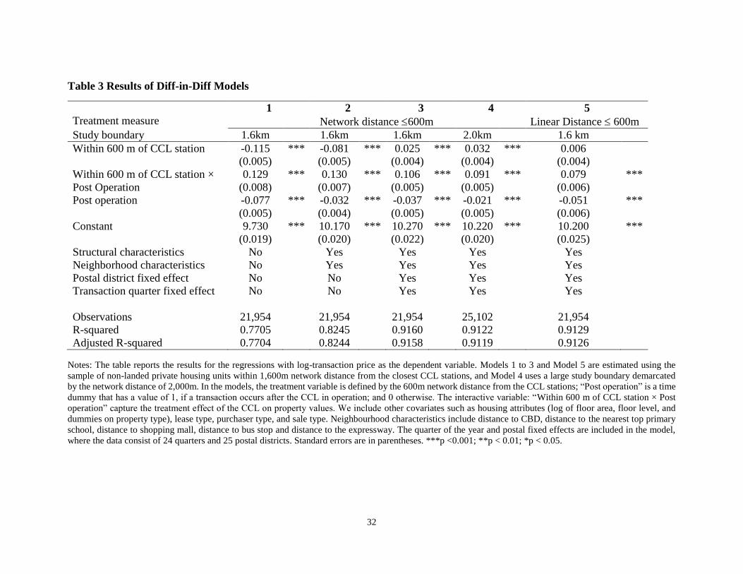
32
Table 3 Results of Diff-in-Diff Models
1 2 3 4 5
Treatment measure Network distance 600m Linear Distance 600m
Study boundary 1.6km 1.6km 1.6km 2.0km 1.6 km
Within 600 m of CCL station -0.115 *** -0.081 *** 0.025 *** 0.032 *** 0.006
(0.005) (0.005) (0.004) (0.004) (0.004)
Within 600 m of CCL station ×
Post Operation
0.129 *** 0.130 *** 0.106 *** 0.091 *** 0.079 ***
(0.008) (0.007) (0.005) (0.005) (0.006)
Post operation -0.077 *** -0.032 *** -0.037 *** -0.021 *** -0.051 ***
(0.005) (0.004) (0.005) (0.005) (0.006)
Constant 9.730 *** 10.170 *** 10.270 *** 10.220 *** 10.200 ***
(0.019) (0.020) (0.022) (0.020) (0.025)
Structural characteristics No Yes Yes Yes Yes
Neighborhood characteristics No Yes Yes Yes Yes
Postal district fixed effect No No Yes Yes Yes
Transaction quarter fixed effect No No Yes Yes Yes
Observations 21,954 21,954 21,954 25,102 21,954
R-squared 0.7705 0.8245 0.9160 0.9122 0.9129
Adjusted R-squared 0.7704 0.8244 0.9158 0.9119 0.9126
Notes: The table reports the results for the regressions with log-transaction price as the dependent variable. Models 1 to 3 and Model 5 are estimated using the
sample of non-landed private housing units within 1,600m network distance from the closest CCL stations, and Model 4 uses a large study boundary demarcated
by the network distance of 2,000m. In the models, the treatment variable is defined by the 600m network distance from the CCL stations; “Post operation” is a time
dummy that has a value of 1, if a transaction occurs after the CCL in operation; and 0 otherwise. The interactive variable: “Within 600 m of CCL station × Post
operation” capture the treatment effect of the CCL on property values. We include other covariates such as housing attributes (log of floor area, floor level, and
dummies on property type), lease type, purchaser type, and sale type. Neighbourhood characteristics include distance to CBD, distance to the nearest top primary
school, distance to shopping mall, distance to bus stop and distance to the expressway. The quarter of the year and postal fixed effects are included in the model,
where the data consist of 24 quarters and 25 postal districts. Standard errors are in parentheses. ***p <0.001; **p < 0.01; *p < 0.05.

33
Table 4 Robustness Tests: Network Distance and Local Polynomial Effects
1 2 3 4
Study boundary 0.6km 1.6km 1.6km 1.6km
Treat(0-300m) 0.027 *** 0.063 *** 0.061 ***
(0.006) (0.007) (0.007)
Treat(300-600m) 0.013 ** 0.010 *
(0.004) (0.005)
Treat(0-600m) 0.025 ***
(0.005)
Treat(600-1000m) 0.000 -0.005
(0.005) (0.005)
Interactive variable:
Treat(0-300m) × Post
operation
0.047 *** 0.125 *** 0.129 ***
(0.008) (0.008) (0.008)
Treat(300-600m) ×
Post operation
0.075 *** 0.080 ***
(0.006) (0.007)
Treat(0-600m)× Post
operation
0.111 ***
(0.006)
Treat(600 -1000m) ×
Post operation
0.009 0.008
(0.006) (0.006)
Post operation -0.036 *** -0.042 *** -0.032 *** -0.037 ***
(0.006) (0.006) (0.005) (0.006)
Constant 10.020 *** 10.260 *** 10.260 *** 10.260 ***
(0.069) (0.023) (0.022) (0.023)
Structural
characteristics
Yes Yes Yes Yes
Neighborhood
characteristics
Yes Yes Yes Yes
Postal district fixed
effect
Yes Yes Yes Yes
Transaction quarter
fixed effect
Yes Yes Yes Yes
Observations 7,388 21,954 21,954 21,954
R-squared 0.9193 0.9160 0.9172 0.9172
Adjusted R-squared 0.9187 0.9158 0.9170 0.9170 Notes: The table reports the results for the regressions with log-transaction price as the dependent variable. The
Models are estimated using the sample of non-landed private housing units within 1,600m network distance
from the closest CCL stations. In the models, the treatment variable is defined by different network distances
from the CCL stations, “Treat( k)”, where [k = (0-300m, 300-600m, 0-600m and 600-1000m)]; “Post operation”
is a time dummy that has a value of 1, if a transaction occurs after the CCL in operation; and 0 otherwise. The
interactive variables: “Treat(k) × Post operation” capture the treatment effect of the CCL on property values.
We include other covariates such as housing attributes (log of floor area, floor level, and dummies on property
type), lease type, purchaser type, and sale type. Neighbourhood characteristics include distance to CBD, distance
to the nearest top primary school, distance to shopping mall, distance to bus stop and distance to the expressway.
The quarter of the year and postal fixed effects are included in the model, where the data consist of 24 quarters
and 25 postal districts. Standard errors are in parentheses. ***p <0.001; **p < 0.01; *p < 0.05.

34
Table 5 Tests of “Anticipation” Effects of the CCL Opening
1 2 3
Sample period 2007-2013 2007-2013 2007-2013
Within 600 m of CCL station -0.064 *** -0.033 *** -0.034 ***
(0.006) (0.006) (0.006)
Postt– 12 -0.061 **
(0.020)
Postt– 6 -0.225 *** -0.214 ***
(0.026) (0.026)
Postt=0 -0.026 ***
(0.005)
Within 600 m of CCL station ×
Postt – 12
0.166 ***
(0.006)
Within 600 m of CCL station ×
Postt– 6
0.136 *** 0.098 ***
( ?) ( ?)
Within 600 m of CCL station ×
Postt=0
0.064 ***
(0.006)
Constant 10.310 *** 10.290 *** 10.280 ***
(0.022) (0.022) (0.022)
Structural characteristics Yes Yes Yes
Neighborhood characteristics Yes Yes Yes
Postal district fixed effect Yes Yes Yes
Transaction quarter fixed effect Yes Yes Yes
Observations 21,954 21,954 21,954
R-squared 0.9168 0.9165 0.9170
Adjusted R-squared 0.9166 0.9163 0.9167
Notes: The table reports the results for the regressions with log-transaction price as the dependent variable.
The Models are estimated using the sample of non-landed private housing units within 1,600m network
distance from the closest CCL stations. In the models, the treatment variable is defined by the 600m network
distance from the CCL stations; “Postt=0” is a time dummy that indicate the opening of Phase 1 of the CCL
in May 2009. For the tests of “anticipation” effects, we include two other time dummies: “Postt-12” and “Postt-
6”, which represent the 12 months and 6 months pre-CCL Phase 1 opening event dates, respectively. The
interactive variable: “Within 600 m of CCL station × Postt-k”, where k=(0, 6, 12), capture the treatment effect
of the CCL on property values. We include other covariates such as housing attributes (log of floor area, floor
level, and dummies on property type), lease type, purchaser type, and sale type. Neighbourhood
characteristics include distance to CBD, distance to the nearest top primary school, distance to shopping mall,
distance to bus stop and distance to the expressway. The quarter of the year and postal fixed effects are
included in the model, where the data consist of 24 quarters and 25 postal districts. Standard errors are in
parentheses. ***p <0.001; **p < 0.01; *p < 0.05.
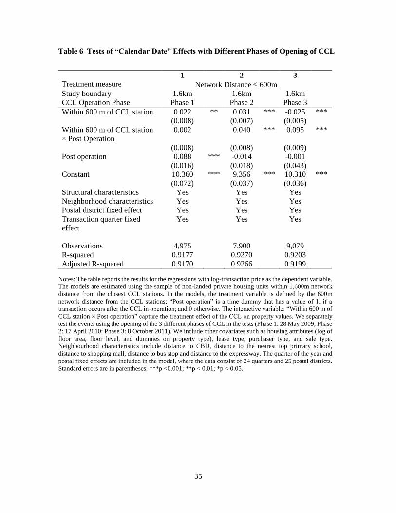
35
Table 6 Tests of “Calendar Date” Effects with Different Phases of Opening of CCL
1 2 3
Treatment measure Network Distance 600m
Study boundary 1.6km 1.6km 1.6km
CCL Operation Phase Phase 1 Phase 2 Phase 3
Within 600 m of CCL station 0.022 ** 0.031 *** -0.025 ***
(0.008) (0.007) (0.005)
Within 600 m of CCL station
× Post Operation
0.002 0.040 *** 0.095 ***
(0.008) (0.008) (0.009)
Post operation 0.088 *** -0.014 -0.001
(0.016) (0.018) (0.043)
Constant 10.360 *** 9.356 *** 10.310 ***
(0.072) (0.037) (0.036)
Structural characteristics Yes Yes Yes
Neighborhood characteristics Yes Yes Yes
Postal district fixed effect Yes Yes Yes
Transaction quarter fixed
effect
Yes Yes Yes
Observations 4,975 7,900 9,079
R-squared 0.9177 0.9270 0.9203
Adjusted R-squared 0.9170 0.9266 0.9199
Notes: The table reports the results for the regressions with log-transaction price as the dependent variable.
The models are estimated using the sample of non-landed private housing units within 1,600m network
distance from the closest CCL stations. In the models, the treatment variable is defined by the 600m
network distance from the CCL stations; “Post operation” is a time dummy that has a value of 1, if a
transaction occurs after the CCL in operation; and 0 otherwise. The interactive variable: “Within 600 m of
CCL station × Post operation” capture the treatment effect of the CCL on property values. We separately
test the events using the opening of the 3 different phases of CCL in the tests (Phase 1: 28 May 2009; Phase
2: 17 April 2010; Phase 3: 8 October 2011). We include other covariates such as housing attributes (log of
floor area, floor level, and dummies on property type), lease type, purchaser type, and sale type.
Neighbourhood characteristics include distance to CBD, distance to the nearest top primary school,
distance to shopping mall, distance to bus stop and distance to the expressway. The quarter of the year and
postal fixed effects are included in the model, where the data consist of 24 quarters and 25 postal districts.
Standard errors are in parentheses. ***p <0.001; **p < 0.01; *p < 0.05.

36
Table 7 Spatial Dependence Diff-in-Diff (SDID) Models
0 1 2 3
OLS SAC SARAR SAC/SARAR
Within 600 m of CCL station 0.025 *** 0.031 *** 0.025 *** 0.021 ***
(0.004) (0.004) (0.004) (0.004)
Within 600 m of CCL station * Post Operation 0.106 *** 0.101 *** 0.079 *** 0.078 ***
(0.005) (0.005) (0.005) (0.005)
Post operation -0.037 *** -0.028 *** -0.015 ** -0.017 ***
(0.005) (0.006) (0.005) (0.005)
Constant 10.270 *** 5.208 *** 8.368 *** 11.006 ***
(0.022) (0.652) (2.112) (2.135)
Rho (spatial lag of dependent variable) 0.342 *** -0.192 ***
(0.037) (0.025)
Lambda (spatial error) 0.999 *** 0.999 ***
(0.000) (0.000)
Structural characteristics Yes Yes Yes Yes
Neighborhood characteristics Yes Yes Yes Yes
Postal district fixed effect Yes Yes Yes Yes
Transaction quarter fixed effect Yes Yes Yes Yes
Observations 21,954 21,954 21,954 21,954
AIC -18,045 -18,811 -19,927 -20,005 Notes: The table reports the results for the regressions with log-transaction price as the dependent variable. The Models are estimated using the sample of non-
landed private housing units within 1,600m network distance from the closest CCL stations. In the models, the treatment variable is defined by the 600m network
distance from the CCL stations; “Post operation” is a time dummy that has a value of 1, if a transaction occurs after the CCL in operation; and 0 otherwise. The
interactive variable: “Within 600 m of CCL station × Post operation” capture the treatment effect of the CCL on property values. We include other covariates such
as housing attributes (log of floor area, floor level, and dummies on property type), lease type, purchaser type, and sale type. Neighbourhood characteristics include
distance to CBD, distance to the nearest top primary school, distance to shopping mall, distance to bus stop and distance to the expressway. The quarter of the year
and postal fixed effects are included in the model, where the data consist of 24 quarters and 25 postal districts. Model 1 is estimated using OLS estimator; Model
2 include a spatial lag variable (SAC); Model 3 include a spatial error term (SARAR), and Model 4 include both SAC and SARAR. Standard errors are in
parentheses. ***p <0.001; **p < 0.01; *p < 0.05.

37
Fig. 1. MRT Network and Non-Landed Private Housing Transactions
Note: The Figure shows the map of Singapore, and the darken solid (red line) shows the Circle line MRT stations on the line are represented by dot (en-route
stations) and star (interchange stations); and the light green dot represent the distributions of housing samples along the Circle Line.

Fig. 2. Network distance and Euclidean distance
Note: The figure uses a sample house located at 107 Aljunied Crescent to illustrate the different between the Euclidean
distance (dotted line) and the network distance (solid green line) to the closest MacPherson MRT Station.
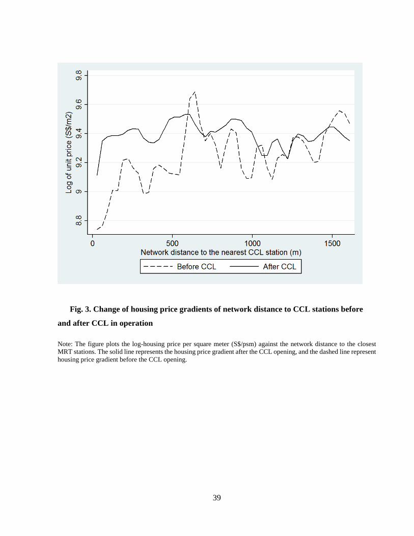
39
Fig. 3. Change of housing price gradients of network distance to CCL stations before
and after CCL in operation
Note: The figure plots the log-housing price per square meter (S$/psm) against the network distance to the closest
MRT stations. The solid line represents the housing price gradient after the CCL opening, and the dashed line represent
housing price gradient before the CCL opening.

40
Fig. 4. Temporal changes of unit price in the treatment and control zones
Note: the Figure plots the price gradients (by log-unit housing price) for the two sets of sample houses, which include
the treatment sample (within 600m from the CCL stations) (solid line) and the control sample (beyond 600m from the
CCL stations) (dashed line), over time (by month from March 2007) (represented by the X-axis). The three vertical
lines represent the opening of the CCL in three different phases.

41
Appendix 1: Local Polynomial Regression (LPR)
Local polynomial regression is a nonparametric regression method widely applied to smooth
scatterplot without making assumptions about the functional form of the expected value of a
response to a given regressor. It involves fitting the response to a polynomial form of the regressor
via locally weighted least squares.
Consider a set of scatterplot data {(𝑥1, 𝑦1), … , (𝑥𝑛, 𝑦𝑛)} from the model:
𝑦𝑖 = 𝑚(𝑥𝑖) + 𝜎(𝑥𝑖)𝜖𝑖
for some unknown mean and variance functions 𝑚(∙) and 𝜎2(∙), and symmetric errors 𝜖𝑖 with
𝐸(𝜖𝑖) = 0 and 𝑉𝑎𝑟(𝜖𝑖) = 1 . The goal is to estimate 𝑚(𝑥0) = 𝐸[𝑌|𝑋 = 𝑥0] , making no
assumptions about the functional form of 𝑚(∙). Local polynomial regression estimate 𝑚(𝑥0) as the
constant term (intercept) of regression, weighted by the kernel function, of y on the polynomial
terms (𝑥 − 𝑥0), (𝑥 − 𝑥0)2, …, (𝑥 − 𝑥0)𝑝 for each smoothing point 𝑥0.
Reference source: http://www.stata.com/manuals13/rlpoly.pdf

42
Appendix 2: MRT Stations on the Circle Line
No Name of Station MRT Station
Code
Interchange
Code
Connecting to
Phase 1 (Opening Date: 28 May 2009)
1 Bartley CC12
2 Serangoon CC13 NE12 / CC13 North-East Line
3 Lorong Chuan CC14
4 Bishan CC15 NS17 / CC15 North-South Line
5 Marymount CC16
Phase 2 (Opening Date: 17 April 2010)
6 Dhoby Ghaut CC1 NS24 / NE6 /
CC1
North-South/North-East
Lines
7 Bras Basah CC2
8 Esplanade CC3
9 Nicoll Highway CC5
10 Stadium CC6
11 Mountbatten CC7
12 Dakota CC8
13 Paya Lebar CC9 EW8 / CC9 East-West Line
14 Macpherson CC10
15 Tai Seng CC11
Phase 3 (Opening Date: 8 October 2011)
16 Caldecott CC17
17 Bukit Brown# CC18
18 Botanic Gardens CC19
19 Farrer Road CC20
20 Holland Village CC21
21 Buona Vista CC22 CC22/EW21 East-West Line
22 One North CC23
23 Kent Ridge CC24
24 Haw Par Villa CC25
25 Pasir Panjang CC26
26 Labrador CC27
27 Telok Blangah CC28
28 Harborfront CC29 CC29/NE1 North-East line
Circle Line Extension (14 January 2012)
29 Marina Bay CC30 NS27 / CE2 /
TS20
North-South Line
/Terminal
30 Bayfront CE1 CE1/DT16 Terminal / Downtown
Line
Note: The stations in the Circle Line Extension opened on 14 January 2012 are not included in the study. # Bukit
Brown station is also closed and reserved for future operation, and not included in our study. There are 3 more new
stations being planned on the CCL (Keppel, Cantoment, and Prince Edward); and construction is scheduled to start in
2018, and the stations will open in 2025, which will complete the loop of CCL upon completion.