Embed Size (px)
Citation preview
r.com/locate/regec
Regional Science and Urban Economics 36 (2006) 727–752www.elsevie
Spatial determinants of productivity: Analysis for theregions of Great Britain
Patricia Rice a,⁎, Anthony J. Venables b,c, Eleonora Patacchini d
a Department of Economics, University of Southampton, Southampton, SO17 1BJ, UKb Department of Economics, London School of Economics, Houghton Street, London WC2A 2AE, UK
c CEPR, UKd La Sapienza, Rome, Italy
Accepted 31 March 2006Available online 7 July 2006
Abstract
This paper uses NUTS3 sub-regional data for Great Britain to analyse the determinants of spatialvariations in income and productivity. We decompose the spatial variation of earnings into a productivityeffect and an occupational composition effect. For the former (but not the latter) we find a robustrelationship with proximity to economic mass, suggesting that doubling the population of working ageproximate to an area is associated with a 3.5% increase in productivity in the area. We measure proximityby travel time, and show that effects decline steeply with time, ceasing to be important beyondapproximately 80 min.© 2006 Elsevier B.V. All rights reserved.
JEL classification: R1; O4Keywords: Regional disparities; Productivity; Clustering
1. Introduction
Regional inequalities are a striking and persistent feature of many economies, developed andless developed. This paper investigates the determinants of spatial productivity differences,paying particular attention to the role of proximity to economic mass. Is it the case, as suggestedby many theories of economic geography, that proximity to centres of economic activity increasesmeasured productivity?
⁎ Corresponding author.E-mail addresses: [email protected] (P. Rice), [email protected] (A.J. Venables).URL: http://econ.lse.ac.uk/staff/ajv/ (A.J. Venables).
0166-0462/$ - see front matter © 2006 Elsevier B.V. All rights reserved.doi:10.1016/j.regsciurbeco.2006.03.006
728 P. Rice et al. / Regional Science and Urban Economics 36 (2006) 727–752
Our analysis is based on the regions of Great Britain. The persistence of significant disparitiesin economic performance across the British regions is well documented, with GDP per capita inLondon in 2001 being 54% above the national average, and even higher in Inner London (ONS,2003). By comparison, GDP per capita in the North East, the poorest of the regions, is just 73% ofthe national average, falling to as low as 60% of the national average in certain sub-regions.Moreover, these disparities have increased over the period 1995 to 2001 with GDP per head inLondon and the South East growing relative to that in regions on the periphery — Scotland, theNorth-East and North West, Wales and the South West.
This paper focuses on regional variations in income per worker, particularly earnings, and asksthree main questions. The first is to what extent are regional inequalities a consequence ofvariation in the quality of jobs, as distinct from variation in productivity in a given type of job?The second relates to the determinants of performance across areas: are differences inperformance related to proximity to centres of activity, as hypothesised by many theories oflocation and spatial clustering? And third, what is the spatial scale of these effects? We base ouranalysis on travel times, and seek to quantify exactly what is meant by ‘proximity’.
The study uses data on the NUTS3 sub-regions of Great Britain.1 The first question isaddressed by decomposing the average earnings of each area into a productivity index and anoccupational composition index. We find that about two-thirds of the spatial variance in earningsis attributable to variations in productivity, although the two indices are positively correlated, sothat there is a tendency for high productivity areas to benefit also from a larger share of jobs inhigh-paying occupations. This earnings decomposition is valuable also because of the importanceof controlling for occupation and skill levels in assessing regional productivity. Ourdecomposition provides a primary control, conditioning out the effects on earnings of spatialvariation in occupational structure.
We address the second and third questions by econometrically investigating the determinantsof spatial variation in a number of measures of economic performance, including the productivityindex and the occupational composition index. The investigation is based on arguments from theeconomic geography literature suggesting that performance is associated with proximity to‘economic mass’. Access to economic mass is measured on the basis of population of working agewithin a series of driving time bands around each area. This rich modelling of the spatial structureof economic mass enables us to estimate both the spatial scale over which economic mass effectsoperate, and their overall impact on productivity.
We find considerable support for the hypothesis that proximity to economic mass raisesincome. The effects operate through the productivity index, rather than through the occupationalcomposition index. Our best estimate of the elasticity of productivity with respect to economicmass is 0.05, suggesting that doubling mass raises productivity by 3.5% (since 20.05 =1.035).These results are robust to the inclusion of a range of additional controls and to the use ofalternative estimators to allow for endogeneity and spatial autocorrelation. Moreover, they are notdriven entirely by London and the south-east, as we demonstrate by splitting the sample ofregions into a south-east core that is within 180 min driving time of London, and the rest. As forspatial scale, effects are greatest for mass within 40 min driving time, tapering off quite sharplythereafter and having little or no effect beyond approximately 80 min. An individual within30 min driving time has four times the impact of an individual 60 min away, and 17 times that ofan individual at 90 min.
1 Nomenclature Unites Territoriales, as reported by Eurostat (e.g. Regio database, Eurostat 1992). Great Britaincontains 126 areas at the NUTS3 level of aggregation and 10 at the NUTS1 level.
729P. Rice et al. / Regional Science and Urban Economics 36 (2006) 727–752
Our results on the overall impact of economic mass on productivity are consistent with, and atthe lower end of, the range of studies surveyed in Rosenthal and Strange (2004). They report aconsensus view (drawn largely from US studies) that the elasticity of city productivity withrespect to city size is in the range 0.04–0.11. For Europe, Ciccone (2002) estimates an elasticity ofproductivity with respect to employment density of around 0.05, while Fingleton (2003) reports afigure of 0.015 for Great Britain. Studies based on earnings data at the individual level typicallyfind somewhat smaller, although still significant, urban wage premia, for example Glaeser andMare (2002) and Combes et al. (2004).2 Wheaton and Lewis (2002) look at wages by occupationand by industry, and find significant and large wage gains for workers in cities with a high share ofemployment in the same occupation or industry. Our findings concerning the steep spatial decayof these effects are also consistent with the small literature addressing this issue (see Section 6below).
The present paper extends the literature in several directions. Our focus on an earnings basedproductivity measure increases the precision of estimates compared to the measures of gross valueadded per worker or average pay that are frequently used. Furthermore, the decomposition ofearnings into an occupational composition index and productivity index demonstrates howeconomic mass is important primarily for the latter, while skill levels are important primarily forthe former. Importantly, the detailed modelling of proximity (measured by driving time) toeconomic mass is more general than the measures of population density in the own orneighbouring regions that are used in much of the literature.3 This enables us to deriveeconomically meaningful estimates of the spatial scale over which the productivity effects ofagglomeration operate.
The paper is organised as follows. The next section covers data and descriptive issues, andderives the decomposition of earnings into occupational composition effects and productivityeffects. The main analysis is reported in Section 3, and Section 4 addresses endogeneity issuesand presents instrumental variable estimates. In Section 5 we explore the role of London and theSouth East of England, and briefly explore differences across occupations. Section 6 quantifiesthe effects we have found, and discusses a number of counterfactual experiments showing, forexample, that a 10% reduction in all travel times in the UK would raise average productivity by1.2%.
2. Regional income, earnings and productivity
Our analysis is based on area-level data for the subregional NUTS3 spatial units of GreatBritain. There are 126 such units in Great Britain but, in order to compile a consistent dataset, anumber of these are combined to give a sample of 119 subregional units that we will term ‘areas’.We use area-level data for the period 1998 to 2001 with the 4 years of data averaged in order toremove some of the year-to-year volatility. Full details of the sample and the data series can befound in the Data Appendix to this paper.
2 Individual level data allows better control for individual characteristics, for example, identifying effects fromindividuals who migrate into cities. Substantial urban wage premia remain.3 For example, Ciccone and Hall (1996) use a US state level density index constructed as an aggregate of the density of
employment in each county in the state. Ciccone (2002) uses NUTS3 employment density and average density incontiguous NUTS3 regions, both instrumented by land areas. Fingleton (2003) uses employment density and a spatial lagof employment density, this derived from a model where wages are determined by employment density and efficiencydetermined by labour skills, technical knowledge and distance weighted efficiency in other areas.
730 P. Rice et al. / Regional Science and Urban Economics 36 (2006) 727–752
There are two main sources of income data at the NUTS 3 level. The Office of NationalStatistics produces estimates of workplace-based gross value-added (GVA) calculated accordingto the income approach (ONS, 2003). From this we construct a measure of GVA per hour workedby employees, using as the denominator an estimate of the total hours worked for the area derivedfrom data on the numbers of full-time and part-time employees and their hours worked. Onedrawback of GVA as a measure of income in these quite small areas is that it is sensitive to thespatial allocation of profits and other non-wage income (see ONS, 2003 for details). The otherincome measure, and that on which we concentrate, is the average hourly earnings of full-timeworkers derived from the workplace-based New Earnings Survey data.
Spatial variation in average earnings derives from two sources — differences in the wage ratespaid to workers in a given occupation, and differences in the occupational composition ofemployment. These two contributions to the spatial structure of average earnings can be separatedout by the following mechanical decomposition.4 wi
k and lik denote the wage and level of
employment in occupation k and area i. Total employment in area i is Li=Σklik, and the share of
occupation k in employment in this area is λik= li
k /Li. The average wage of occupation k in theeconomy as a whole (i.e. aggregating across all i) is given by w k=Σili
kwik /Σili
k, while λ¯k=Σilik /ΣiLi
is the share of occupation k in total employment for the economy as a whole. Average earnings inarea i, ei, may therefore be decomposed as
eiuRkwki k
ki ¼ Rkw
ki k¯k þ Rk w
kkki þ Rkðwki − w
kÞðkki −k¯kÞ−Rk w
kk¯k: ð1Þ
The first term on the right-hand side of Eq. (1) is the average level of earnings at location iconditional on the occupational composition being the same as for the economy as a whole. It will bedenoted qi≡Σkwi
kλk, andwe refer to qi as the productivity index, aswill be discussed further in Section3. The second term is the average level of earnings of area i given its occupational composition butassuming that the wage rate for each occupation equals the GB average in that occupation. It will bedenoted ci≡Σkw
kλik, and referred to as the occupational composition index.Remaining termsmeasure
the covariance between wages and occupational shares in area i, and will be denoted ri.We compute the productivity index and the occupational composition index as specified above
for each of the NUTS 3 areas of Great Britain. The value of the method rests on being able tocompute the indices at a sufficiently disaggregate level that the occupational categories arerelatively homogeneous. The productivity index, qi, is constructed from data on earnings byoccupation for each of 38 minor occupational groups taken from the workplace-based NewEarnings Surveys. The weights are the shares of each occupation in the total employment of GreatBritain as a whole and these are computed from Labour Force Survey data. The productivity index,qi, like the measures of GVA per hour worked and of average hourly earnings described above, istherefore workplace-based. The composition index, ci, requires data on employment shares foreach occupation which is available from the Labour Force Survey with two important limitations.First, sample sizes are such that, once disaggregated to the level of a NUTS3 area, reliableestimates of employment shares are available only for the 9 major occupational groups. Second,the Labour Force Survey is residence-based, rather than workplace-based and this limits directcomparability with the measures of income and productivity discussed above. For these reasons,we attach rather less significance to the results relating to the occupational composition index.
4 We decompose spatial variations in levels of variables. When applied to changes this corresponds to ‘shift-share’analysis, see e.g. Dunn (1960), Estaban (2000).
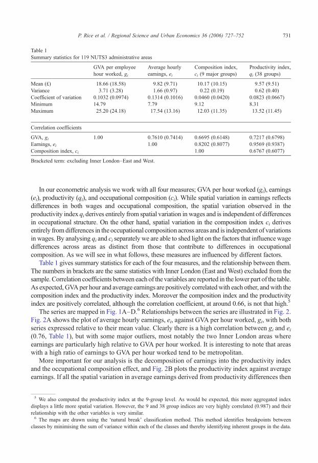
Table 1Summary statistics for 119 NUTS3 administrative areas
GVA per employeehour worked, gi
Average hourlyearnings, ei
Composition index,ci (9 major groups)
Productivity index,qi (38 groups)
Mean (£) 18.66 (18.58) 9.82 (9.71) 10.17 (10.15) 9.57 (9.51)Variance 3.71 (3.28) 1.66 (0.97) 0.22 (0.19) 0.62 (0.40)Coefficient of variation 0.1032 (0.0974) 0.1314 (0.1016) 0.0460 (0.0420) 0.0823 (0.0667)Minimum 14.79 7.79 9.12 8.31Maximum 25.20 (24.18) 17.54 (13.16) 12.03 (11.35) 13.52 (11.45)
Correlation coefficients
GVA, gi 1.00 0.7610 (0.7414) 0.6695 (0.6148) 0.7217 (0.6798)Earnings, ei 1.00 0.8202 (0.8077) 0.9569 (0.9387)Composition index, ci 1.00 0.6767 (0.6077)
Bracketed term: excluding Inner London–East and West.
731P. Rice et al. / Regional Science and Urban Economics 36 (2006) 727–752
In our econometric analysis we work with all four measures; GVA per hour worked (gi), earnings(ei), productivity (qi), and occupational composition (ci). While spatial variation in earnings reflectsdifferences in both wages and occupational composition, the spatial variation observed in theproductivity index qi derives entirely from spatial variation in wages and is independent of differencesin occupational structure. On the other hand, spatial variation in the composition index ci derivesentirely fromdifferences in the occupational composition across areas and is independent of variationsin wages. By analysing qi and ci separately we are able to shed light on the factors that influencewagedifferences across areas as distinct from those that contribute to differences in occupationalcomposition. As we will see in what follows, these measures are influenced by different factors.
Table 1 gives summary statistics for each of the four measures, and the relationship between them.The numbers in brackets are the same statistics with Inner London (East andWest) excluded from thesample. Correlation coefficients between each of the variables are reported in the lower part of the table.As expected,GVAper hour and average earnings are positively correlatedwith each other, andwith thecomposition index and the productivity index. Moreover the composition index and the productivityindex are positively correlated, although the correlation coefficient, at around 0.66, is not that high.5
The series are mapped in Fig. 1A–D.6 Relationships between the series are illustrated in Fig. 2.Fig. 2A shows the plot of average hourly earnings, ei, against GVA per hour worked, gi, with bothseries expressed relative to their mean value. Clearly there is a high correlation between gi and ei(0.76, Table 1), but with some major outliers, most notably the two Inner London areas whereearnings are particularly high relative to GVA per hour worked. It is interesting to note that areaswith a high ratio of earnings to GVA per hour worked tend to be metropolitan.
More important for our analysis is the decomposition of earnings into the productivity indexand the occupational composition effect, and Fig. 2B plots the productivity index against averageearnings. If all the spatial variation in average earnings derived from productivity differences then
5 We also computed the productivity index at the 9-group level. As would be expected, this more aggregated indexdisplays a little more spatial variation. However, the 9 and 38 group indices are very highly correlated (0.987) and theirrelationship with the other variables is very similar.6 The maps are drawn using the ‘natural break’ classification method. This method identifies breakpoints between
classes by minimising the sum of variance within each of the classes and thereby identifying inherent groups in the data.
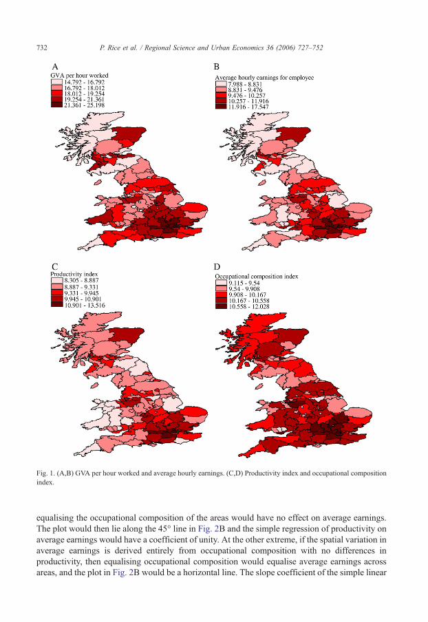
Fig. 1. (A,B) GVA per hour worked and average hourly earnings. (C,D) Productivity index and occupational compositionindex.
732 P. Rice et al. / Regional Science and Urban Economics 36 (2006) 727–752
equalising the occupational composition of the areas would have no effect on average earnings.The plot would then lie along the 45° line in Fig. 2B and the simple regression of productivity onaverage earnings would have a coefficient of unity. At the other extreme, if the spatial variation inaverage earnings is derived entirely from occupational composition with no differences inproductivity, then equalising occupational composition would equalise average earnings acrossareas, and the plot in Fig. 2B would be a horizontal line. The slope coefficient of the simple linear
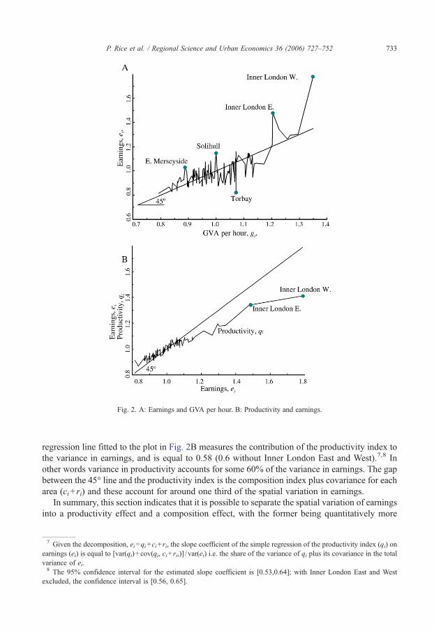
Fig. 2. A: Earnings and GVA per hour. B: Productivity and earnings.
733P. Rice et al. / Regional Science and Urban Economics 36 (2006) 727–752
regression line fitted to the plot in Fig. 2B measures the contribution of the productivity index tothe variance in earnings, and is equal to 0.58 (0.6 without Inner London East and West).7,8 Inother words variance in productivity accounts for some 60% of the variance in earnings. The gapbetween the 45° line and the productivity index is the composition index plus covariance for eacharea (ci+ ri) and these account for around one third of the spatial variation in earnings.
In summary, this section indicates that it is possible to separate the spatial variation of earningsinto a productivity effect and a composition effect, with the former being quantitatively more
7 Given the decomposition, ei=qi+ci+ ri, the slope coefficient of the simple regression of the productivity index (qi) onearnings (ei) is equal to [var(qi)+cov(qi, ci+ ri,)] / var(ei) i.e. the share of the variance of qi plus its covariance in the totalvariance of ei.8 The 95% confidence interval for the estimated slope coefficient is [0.53,0.64]; with Inner London East and West
excluded, the confidence interval is [0.56, 0.65].
734 P. Rice et al. / Regional Science and Urban Economics 36 (2006) 727–752
important. Of course, the separation is not perfect — jobs within an occupation are far fromhomogeneous, even at the level of 38 occupations. Theory suggests that the determinants ofproductivity and of occupational structure are quite different, and we will see this come through inthe econometric analysis of the next section.
3. Explaining regional disparities
3.1. Conceptual framework
We start by outlining a theoretical framework within which interactions between the differentaspects of regional inequality can be placed, and which points to the relationships that we willidentify econometrically. The simplest framework is to suppose that there is a number of tradableactivities (indexed by superscript s) each of which has the same price in all areas, Ps. Individualfirms have constant returns to scale and make zero profits, so the equality of price to unit cost is,for all activities s and areas i,
Ps ¼ bsð½w1i N w
ki N w
Ki �=qi; qÞ; ð2Þ
where bs(.) is the unit cost function in activity s. There are K occupations (types of labour) witharea specific wages wi
k (as in Section 2), and all occupations have the same area specificproductivity parameter qi. Other inputs have the same price in all areas— for example, capital withprice ρ.We shall assume that the number of tradable activities operating in each area is at least asgreat as K, the number of types of labour. This dimensionality assumption allows us to invoke aweak form of ‘factor price equalisation’ result from trade theory.9 The set of equations (Eq. (2))giving equality of price to unit cost can be solved for factor prices. Since they hold in all areas theyimply that wi
k /qi=wjk /qi for each k and for any pair of areas i, j. For our purposes, the point is that
relative productivities are exactly equal to relative factor prices across areas, wik /wj
k=qi /qj.A number of further remarks are in order. First, although the spatial variation in wages is
determined entirely from the production side of the economy this approach is quite consistentwith perfect mobility of labour. If there is perfect labour mobility then any spatial differences inwages (and in other considerations such as amenity or disutility of congestion) will be fullyshifted into the prices of immobile factors in each area—land and housing. We can be quiteagnostic about the extent to which such mobility is possible; any degree of labour mobility isentirely consistent with our approach.10
Second, in general, the approach offers no predictions about the structure of production in eacharea. As we have seen, it is consistent with the different degrees of factor mobility and hencedifferent factor stocks in each region. And furthermore, if there are more tradable activities thanthere are distinct types of labour then factor stocks do not map uniquely into sectoral outputs (seeLeamer, 1984 for details of higher dimensional trade theory). Turning this statement around, ourapproach is consistent with the predictions of alternative theories with regard to regional andurban production structures.11
9 More accurately termed factor price invariance with respect to endowments, see Leamer (1984). Since each area is aprice-taker the theorem implies infinitely elastic demand curves for labour of each type.10 If labour is immobile then we would still observe the same wage differences, although prices of land would notnecessarily have adjusted to give real wage equalisation across regions.11 Models of regional specialisation include the hierarchical view of central place theory, and models of urbanspecialisation (eg Henderson, 1974).
735P. Rice et al. / Regional Science and Urban Economics 36 (2006) 727–752
Third, we have assumed that productivity levels are area specific, but not specific either tosectors or occupations. These assumptions give the benchmark case, and relaxing them addsmore detail but does not change the main conclusion. For example, spatial productivitydifferences may be greater for some types of workers or for some activities than others, in whichcase the model would also provide a theory of regional specialisation. We do not pursue thisfurther, instead focusing just on the overall variation of the productivity of a composite labourinput across areas.
Given this structure, the remaining task is to model the determinants of productivitydifferences across areas. Our main hypothesis is that labour productivity is high in regions thathave, in some sense, proximity to a large economic mass. Three main sorts of mechanisms havebeen put forward for this (see Fujita and Thisse, 2002 for a survey). One is technologicalexternalities; firms learn from co-presence with other firms in related activities, so innovating andimplementing new technologies efficiently. A second is that thick labour markets work moreefficiently, by having lower search costs and generating improved labour market matching. Thethird main mechanism is simply that, in the presence of transport costs, firms gain from havinggood access both to their customers and to suppliers of intermediate goods and services.
We do not seek to identify each of these effects separately, but merely their combined effect byestimating a relationship with general form
yi ¼ f ðxiÞmðRhphahiÞ: ð3Þ
For the dependent variable, yi, we will use all four of the measures outlined in the previous section,while focussing on productivity, qi. Independent variables include a set of controls for each area, xi,and spatial mass effects. ph is a measure of the economic mass of each area, ahi is a measure of theinteraction between area h and area i, and the functionm(.) captures the combined spatial mass effects.For theoretical derivation of particular forms of this equation, see Fujita et al. (1999) or Redding andVenables (2004). The next section estimates several different forms of this relationship, and establishesour main results. However we note that the location of ‘economic mass’may itself be endogenous; inSection 4 we discuss this further and present results estimated using instrumental variables.
3.2. Explaining regional productivity: economic mass by time bands
Our measure of the economic mass of each area, ph, is based on its population of working age.This measure is chosen, in preference to alternatives such as employment, to serve as both anindicator of the potential labour force of an area and of the size the local market. It is central to ourapproach that we capture not only own area effects but also inter-area effects, the interactionterms, ahi. This is important both because NUTS3 areas are relatively small with boundariesdetermined by administrative rather than economic considerations, and in order to understand thespatial scale over which economic mass effects occur. We assume that these interactions are afunction of proximity, and measure this by driving time within and between NUTS3 regions.Driving times are more economically relevant than other measures of proximity, such as distanceor contiguity, and produce slightly better results than do estimates based on geographical distance.
To implement this we form proximity bands based on driving-time around each NUTS3 area,and measure the population of working age within each proximity band. So, for example, wemeasure the population of working age within 40 min driving time of area i; within 40–80 mindriving time of area i, and so on. We construct these bands under two alternative models of thedistribution of population within each NUTS3 area. The first assumes that the population of each
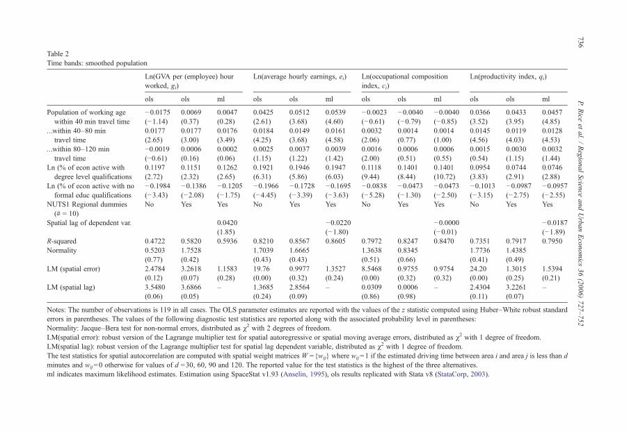
Table 2Time bands: smoothed population
Ln(GVA per (employee) hourworked, gi)
Ln(average hourly earnings, ei) Ln(occupational compositionindex, ci)
Ln(productivity index, qi)
ols ols ml ols ols ml ols ols ml ols ols ml
Population of working agewithin 40 min travel time
−0.0175(−1.14)
0.0069(0.37)
0.0047(0.28)
0.0425(2.61)
0.0512(3.68)
0.0539(4.60)
−0.0023(−0.61)
−0.0040(−0.79)
−0.0040(−0.85)
0.0366(3.52)
0.0433(3.95)
0.0457(4.85)
…within 40–80 mintravel time
0.0177(2.65)
0.0177(3.00)
0.0176(3.49)
0.0184(4.25)
0.0149(3.68)
0.0161(4.58)
0.0032(2.06)
0.0014(0.77)
0.0014(1.00)
0.0145(4.56)
0.0119(4.03)
0.0128(4.53)
…within 80–120 mintravel time
−0.0019(−0.61)
0.0006(0.16)
0.0002(0.06)
0.0025(1.15)
0.0037(1.22)
0.0039(1.42)
0.0016(2.00)
0.0006(0.51)
0.0006(0.55)
0.0015(0.54)
0.0030(1.15)
0.0032(1.44)
Ln (% of econ active withdegree level qualifications
0.1197(2.72)
0.1151(2.32)
0.1262(2.65)
0.1921(6.31)
0.1946(5.86)
0.1947(6.03)
0.1118(9.44)
0.1401(8.44)
0.1401(10.72)
0.0954(3.83)
0.0744(2.91)
0.0746(2.88)
Ln (% of econ active with noformal educ qualifications
−0.1984(−3.43)
−0.1386(−2.08)
−0.1205(−1.75)
−0.1966(−4.45)
−0.1728(−3.39)
−0.1695(−3.63)
−0.0838(−5.28)
−0.0473(−1.30)
−0.0473(−2.50)
−0.1013(−3.15)
−0.0987(−2.75)
−0.0957(−2.55)
NUTS1 Regional dummies(# = 10)
No Yes Yes No Yes Yes No Yes Yes No Yes Yes
Spatial lag of dependent var. 0.0420(1.85)
−0.0220(−1.80)
−0.0000(−0.01)
−0.0187(−1.89)
R-squared 0.4722 0.5820 0.5936 0.8210 0.8567 0.8605 0.7972 0.8247 0.8470 0.7351 0.7917 0.7950Normality 0.5203
(0.77)1.7528(0.42)
1.7039(0.43)
1.6665(0.43)
1.3638(0.51)
0.8345(0.66)
1.7736(0.41)
1.4385(0.49)
LM (spatial error) 2.4784(0.12)
3.2618(0.07)
1.1583(0.28)
19.76(0.00)
0.9977(0.32)
1.3527(0.24)
8.5468(0.00)
0.9755(0.32)
0.9754(0.32)
24.20(0.00)
1.3015(0.25)
1.5394(0.21)
LM (spatial lag) 3.5480(0.06)
3.6866(0.05)
– 1.3685(0.24)
2.8564(0.09)
– 0.0309(0.86)
0.0006(0.98)
– 2.4304(0.11)
3.2261(0.07)
–
Notes: The number of observations is 119 in all cases. The OLS parameter estimates are reported with the values of the z statistic computed using Huber–White robust standarderrors in parentheses. The values of the following diagnostic test statistics are reported along with the associated probability level in parentheses:Normality: Jacque–Bera test for non-normal errors, distributed as χ2 with 2 degrees of freedom.LM(spatial error): robust version of the Lagrange multiplier test for spatial autoregressive or spatial moving average errors, distributed as χ2 with 1 degree of freedom.LM(spatial lag): robust version of the Lagrange multiplier test for spatial lag dependent variable, distributed as χ2 with 1 degree of freedom.The test statistics for spatial autocorrelation are computed with spatial weight matrices W ={wij} where wij=1 if the estimated driving time between area i and area j is less than dminutes and wij=0 otherwise for values of d =30, 60, 90 and 120. The reported value for the test statistics is the highest of the three alternatives.ml indicates maximum likelihood estimates. Estimation using SpaceStat v1.93 (Anselin, 1995), ols results replicated with Stata v8 (StataCorp, 2003).
736P.
Rice
etal.
/Regional
Scienceand
Urban
Econom
ics36
(2006)727–752
737P. Rice et al. / Regional Science and Urban Economics 36 (2006) 727–752
NUTS3 area is massed at the economic centre of the area, which lies entirely within a singleproximity band. The alternative approach assumes that the population is evenly distributed acrossthe area, so may be divided between several proximity bands (‘smoothed population’). Details ofthe procedure for identifying the centres of areas, the estimation of travel times between centres,and the distribution of population within each area are provided in the Appendix.
With this structure, the estimating equation becomes
lnyi ¼ b0 þXb
abpbi þXj
bjxji þ ei ð4Þ
where pbi denotes the population of working age within the proximity band b of area i, and xji isthe value of the jth control variable in area i. In writing Eq. (3) in this way we have assumed aparticular functional form, and allow the data to identify the weights αb for each proximity band.
Table 2 reports the results obtained with three proximity bands; up to 40 min, 40 to 80 min and80 to 120 min, and with smoothed population (appendix Table A1 reports the corresponding‘mass point’ estimates). Additional controls are included to allow for other area specificcharacteristics that may affect outcomes. Variation in the education levels of the local workforce iscontrolled for by including the proportion of the economically active population with specifiedlevels of qualifications.12 The preliminary analysis identified six distinct educational levelsranging from no formal qualifications up to degree level qualifications. These were aggregatedinto three groups to obtain a more parsimonious and statistically robust specification. The threegroups are: first degree or higher (level 4 or above); intermediate levels qualifications (levels 1, 2and 3) and no formal educational qualifications (unqualified or trade qualifications only). Theintermediate qualification level is taken to be the reference group. In addition, a set of dummyvariables for the 10 large NUTS1 regions are included to capture any unobserved region-specificfixed effects.
This model is estimated taking as the dependent variable each of the incomemeasures; GVA perhour worked, gi; average earnings, ei; the occupational composition index, ci; and the productivityindex, qi. The OLS parameter estimates for the model with and without the regional dummies arereported in the first two columns of each of the blocks in Table 2. In the third column we report theresults obtained with the inclusion of a spatially lagged dependent variable as an additionalexplanatory variable.13 This is to allow for the possibility of spatial dependence in the data that isnot fully captured by the population bands. In this case, the model is estimated by maximumlikelihood methods, rather than OLS, to take account of the correlation between the spatiallylagged dependent variable and the error term. Together with the parameter estimates, we report thevalues of the associated z statistics computed using Huber–White robust standard errors.
If we compare the results for the two alternative measures of area income, gi and ei, we findthat the specification using earnings ei as the dependent variable is the better determined, althoughin both cases there is evidence of a significant positive effect of access to economic mass.Focusing on this equation, earnings increase with the population of working age up to a distanceof some 80 min travel time from the centre of the sub-region. The quantitative impact ofpopulation declines with distance, with the coefficients on the 40 to 80 min band significantlysmaller than that for the 0 to 40 min band. Beyond 80 min the population effects are statisticallyinsignificant.
12 Skill effects may operate via composition effects and human capital externalities (see Moretti, 2004).13 The spatial lag of the dependent variable is the average vale of the dependent variable for neighbouring NUTS3 areaswithin a given proximity of the sample point.
738 P. Rice et al. / Regional Science and Urban Economics 36 (2006) 727–752
The next question to be addressed is whether the relationship between earnings and access toeconomic mass comes about through the productivity component, the occupational compositioncomponent, or both. The results are unambiguous. We find no evidence of a significant effectfrom economic mass to occupational composition, particularly once we control for region-specific effects. By contrast, the relationship between economic mass and productivity is strongand well determined. Productivity increases with population within 80 min travel time, and themagnitude of effects are significantly greater the closer population is, i.e. for the 0 to 40 minband compared to the 40 to 80 min band. The magnitude of the population effects is sensitiveto the measurement of population and falls off more sharply with driving time when populationis smoothed across space rather than concentrated at a mass point (comparing Table A1 withTable 2).
Turning to the other variables in the regression equation, the qualification controls arestatistically significant in all cases. As one would expect, a higher proportion of the populationqualified to first degree or higher is associated with a higher level of income in the area asmeasured by GVA per hour worked and by average hourly earnings; while the reverse is true forthe proportion of unqualified workers. If it were possible to control perfectly for occupationalcomposition in the construction of the productivity index then one might expect that the impact ofqualifications on earnings would come only through the composition index, and not at all throughproductivity. While this is not so, it is the case that education levels, and in particular theproportion of population with degree level qualifications, have a much weaker effect onproductivity than on average earnings and on occupational composition.
Along with the parameter estimates and their associated z-values, we report the values ofdiagnostic tests for possible misspecification of the spatial structure of the data. The first is a testfor a spatial process in the error term of the model and the second test is for an omitted spatiallylagged dependent variable.14 In each case, the null hypothesis of no spatial dependence is testedagainst an alternative of spatial dependence within a specified proximity. Proximity is measuredin terms of estimated driving times and the tests are computed for values of 30, 60, 90 and120 min, with the highest values obtained in each case reported in the table. Both tests are validonly under the assumption of normality and so we report also the value of the Jacques–Bera teststatistic for normality of the errors.
The diagnostic statistics show no evidence of a spatial process in the error term of the modelonce regional dummies are included in the specification. There is, however, evidence of anomitted spatial lag in the model for GVA per hour worked and, to a lesser degree, in the equationsfor average hourly earnings and the productivity index, which may lead to bias and inconsistencyin OLS parameter estimates. A comparison of the OLS estimates in column 2 with the MLestimates in column 3 shows that the inclusion of the spatially lagged dependent variables haslittle impact on estimated parameter values. In particular, the parameter estimates on thesuccessive population bands in the earnings and productivity equations are robust to thisparticular form of misspecification; increasing marginally in value and statistical significancewith the inclusion of the spatially-lagged dependent variable.
3.3. Explaining regional productivity: spatial decay
Table 2 indicates that the effect of economic mass on earnings falls away sharply with traveltime. This relationship can be examined further by taking a finer cut on the width of the time
14 For details of the structure of the spatial test statistics see Anselin (1992).
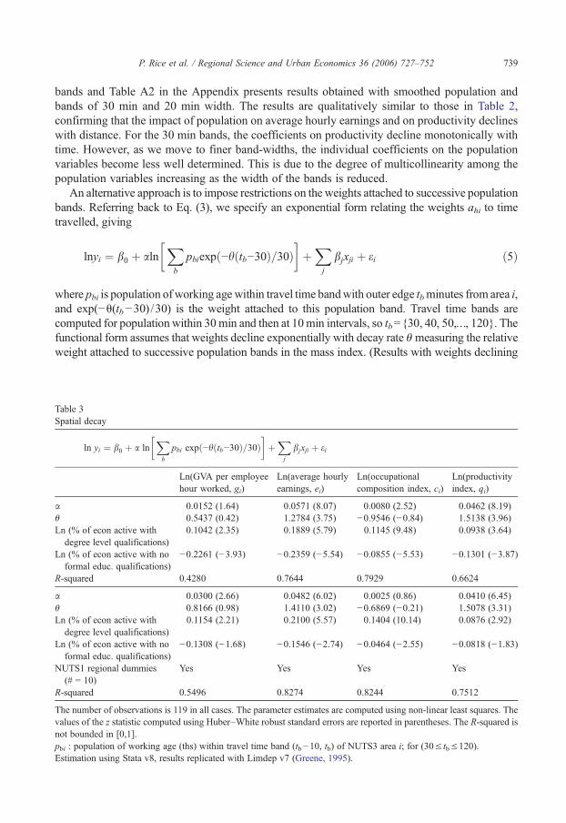
739P. Rice et al. / Regional Science and Urban Economics 36 (2006) 727–752
bands and Table A2 in the Appendix presents results obtained with smoothed population andbands of 30 min and 20 min width. The results are qualitatively similar to those in Table 2,confirming that the impact of population on average hourly earnings and on productivity declineswith distance. For the 30 min bands, the coefficients on productivity decline monotonically withtime. However, as we move to finer band-widths, the individual coefficients on the populationvariables become less well determined. This is due to the degree of multicollinearity among thepopulation variables increasing as the width of the bands is reduced.
An alternative approach is to impose restrictions on the weights attached to successive populationbands. Referring back to Eq. (3), we specify an exponential form relating the weights ahi to timetravelled, giving
lnyi ¼ b0 þ aln
�Xb
pbiexpð−hðtb−30Þ=30Þ�þXj
bjxji þ ei ð5Þ
where pbi is population ofworking age within travel time bandwith outer edge tbminutes from area i,and exp(−θ(tb−30) /30) is the weight attached to this population band. Travel time bands arecomputed for population within 30min and then at 10min intervals, so tb={30, 40, 50,…, 120}. Thefunctional form assumes that weights decline exponentially with decay rate θmeasuring the relativeweight attached to successive population bands in the mass index. (Results with weights declining
Table 3Spatial decay
ln yi ¼ b0 þ a ln
�Xb
pbi expð−hðtb−30Þ=30Þ�þXj
bjxji þ ei
Ln(GVA per employeehour worked, gi)
Ln(average hourlyearnings, ei)
Ln(occupationalcomposition index, ci)
Ln(productivityindex, qi)
α 0.0152 (1.64) 0.0571 (8.07) 0.0080 (2.52) 0.0462 (8.19)θ 0.5437 (0.42) 1.2784 (3.75) −0.9546 (−0.84) 1.5138 (3.96)Ln (% of econ active with
degree level qualifications)0.1042 (2.35) 0.1889 (5.79) 0.1145 (9.48) 0.0938 (3.64)
Ln (% of econ active with noformal educ. qualifications)
−0.2261 (−3.93) −0.2359 (−5.54) −0.0855 (−5.53) −0.1301 (−3.87)
R-squared 0.4280 0.7644 0.7929 0.6624
α 0.0300 (2.66) 0.0482 (6.02) 0.0025 (0.86) 0.0410 (6.45)θ 0.8166 (0.98) 1.4110 (3.02) −0.6869 (−0.21) 1.5078 (3.31)Ln (% of econ active with
degree level qualifications)0.1154 (2.21) 0.2100 (5.57) 0.1404 (10.14) 0.0876 (2.92)
Ln (% of econ active with noformal educ. qualifications)
−0.1308 (−1.68) −0.1546 (−2.74) −0.0464 (−2.55) −0.0818 (−1.83)
NUTS1 regional dummies(# = 10)
Yes Yes Yes Yes
R-squared 0.5496 0.8274 0.8244 0.7512
The number of observations is 119 in all cases. The parameter estimates are computed using non-linear least squares. Thevalues of the z statistic computed using Huber–White robust standard errors are reported in parentheses. The R-squared isnot bounded in [0,1].pbi : population of working age (ths) within travel time band (tb−10, tb) of NUTS3 area i; for (30≤ tb≤120).Estimation using Stata v8, results replicated with Limdep v7 (Greene, 1995).
740 P. Rice et al. / Regional Science and Urban Economics 36 (2006) 727–752
linearly rather than exponentially are given in appendix Table A3). The parameter α measures theelasticity with respect to the mass index as a whole. The parameters, α and θ, together with the βj forthe additional controls, are estimated using non-linear least squares. Table 3 reports results obtainedfor this specification both with regional dummies (lower panel) and without (upper panel). We usesmoothed population estimates but the results obtained with mass point population estimates arequantitatively very similar.
These results confirm our earlier findings. As before, the relationship with economic massis better determined with average hourly earnings than with a GVA-based measure of income.That said, the estimated elasticity of GVA per hour worked with respect to economic mass ispositive and statistically significant when regional dummies are included although the estimateof θ is not well determined. Most importantly, we find that the effects of economic mass onincome come about through productivity, rather than through occupational composition. Withthe inclusion of regional dummies, neither the estimate of α (the elasticity with respect to themass index) nor the estimate of θ is statistically significant in the estimating equation for theoccupational composition index. By contrast, the estimated elasticity of the productivity indexwith respect to economic mass is 0.041 (0.046 without regional dummies) and is very well-determined. Similarly, the estimate of θ indicates that effects decline with distance, and iswell-determined.
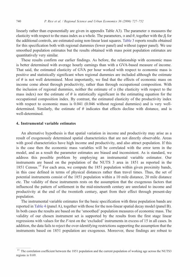
4. Instrumental variable estimates
An alternative hypothesis is that spatial variation in income and productivity may arise as aresult of exogenously determined spatial characteristics that are not directly observable. Areaswith good characteristics have high income and productivity, and also attract population. If thisis the case then the economic mass variables will be correlated with the error term in themodel, and as a result the parameter estimates are biased and inconsistent. As is standard, weaddress this possible problem by employing an instrumental variable estimator. Ourinstruments are based on the population of the NUTS 3 area in 1851 as reported in the1851 Census.15 For each area, we compute the 1851 population within given proximity bands,in this case defined in terms of physical distances rather than travel times. Thus, the set ofpotential instruments consist of the 1851 population within a 10 mile distance, 20 mile distanceetc. The validity of these instruments rests on the assumption that the exogenous factors thatinfluenced the pattern of settlement in the mid-nineteenth century are unrelated to income andproductivity at the end of the twentieth century, apart from their effect through present-daypopulation.
The instrumental variable estimates for the basic specification with three population bands arereported in Table 4 (panel A), together with those for the non-linear spatial decay model (panel B).In both cases the results are based on the ‘smoothed’ population measures of economic mass. Thevalidity of our chosen instrument set is supported by the results from the first stage linearregressions with values for the F-test on the ‘excluded’ instruments in excess of 15 in all cases. Inaddition, the data fails to reject the over-identifying restrictions supporting the assumption that theinstruments based on 1851 population are exogenous. Moreover, these findings are robust to
15 The correlation coefficient between the 1851 population and the current population of working age across the NUTS3regions is 0.69.
Table 4Instrumental variable estimates
(A) Linear Model
Ln(GVA per (employee)hour worked, gi)
Ln(average hourlyearnings, ei)
Ln(occupationalcomposition index, ci)
Ln(productivityindex, qi)
Population of working agewithin 40 min travel time
−0.0370 (−1.37) 0.0584 (2.02) −0.0054 (−0.69) 0.0492 (2.46)
...within 40–80 min traveltime
0.0257 (3.62) 0.0133 (2.06) 0.0021 (0.94) 0.0097 (2.19)
...within 80–120 mintravel time
−0.0031 (−0.57) 0.0070 (1.57) 0.0022 (1.33) 0.0051 (1.33)
Ln (% of ec. active withdegree level qualifications
0.1282 (2.45) 0.1866 (5.53) 0.1371 (9.18) 0.0690 (2.66)
Ln (% of ec. active with noformal educ. qualifications
−0.1463 (−2.09) −0.1693 (−3.69) −0.0449 (−2.17) −0.098 (−2.99)
NUTS1 regional dummies(# = 10)
Yes Yes Yes Yes
R-squared 0.5535 0.8542 0.8424 0.7862Test of over-identifying
restrictions: χ2(2)0.187 0.005 0.208 1.147
Number of observations=119Instruments: 1851 population in the area within 10 miles; within 20 miles; within 40 miles; within 50 miles; within80 miles; Ln (% of economically active population with degree level qualifications); Ln (% of economically activepopulation with no formal educational qualifications); regional dummies.Summary statistics for first stage regressions: F tests for the ‘excluded’ instrumentsPopulation of working age within 40 min travel time: F(6,100)=15.76Population of working age within 40–80 min travel time: F(6,100)=60.90Population of working age within 80–120 min travel time: F(6,100)=22.65
(B) Spatial Decay Model
ln yi ¼ b0 þ a ln
�Xb
pbi expð−hðtb−30Þ=30Þ�þXj
bjxji þ ei
α 0.0438 (3.10) 0.0698 (6.68) 0.0101 (2.47) 0.0530 (6.42)θ 0.5662 (0.80) 1.2045 (2.85) −0.2253 (−0.20) 1.3714 (2.96)Ln (% of econ active with
degree level qualifications)0.1160 (2.35) 0.2134 (5.84) 0.1404 (10.44) 0.0898 (3.14)
Ln (% of econ active with noformal educ. qualifications)
−0.1134 (−1.52) −0.1231 (−2.22) −0.0377 (−1.89) −0.0641 (−1.48)
NUTS1 regional dummies Yes Yes Yes YesR-squared 0.5466 0.8167 0.8368 0.7447
Number of observations=119.Instruments: 1851 population in the area within each 10-mile distance band between 10 and 80 miles; Ln (% ofeconomically active population with degree level qualifications); Ln (% of economically active population withno formal educational qualifications); regional dummies. The R-squared statistic is not bounded in [0,1].Estimation using Limdep v7, results for linear IV replicated using Stata v8.
741P. Rice et al. / Regional Science and Urban Economics 36 (2006) 727–752
variations in the instrument set to include alternative ranges of 1851 population bands and othergeographical-based measures such as distance from London.
The IV estimates confirm the main findings from earlier tables. In general, the IV estimates ofthe elasticity with respect to economic mass in Table 4 are somewhat larger than their LS
742 P. Rice et al. / Regional Science and Urban Economics 36 (2006) 727–752
counterparts in Tables 2 and 3. For example, the IV estimate of α (the elasticity with respect toeconomic mass in the spatial decay model) for the productivity index is 0.0530, as compared withthe NLS estimate is 0.0410. By contrast, the IVestimate of θ, the rate of decay, is smaller than itsNLS counterpart; 1.37 as compared with 1.51.
We take the estimate of α=0.053 as our benchmark estimate of the elasticity of productivitywith respect to economic mass, and we use it in Section 6 to assess the quantitative importance ofthese productivity effects. But before doing this we investigate further the robustness of ourresults, investigating the possibility that effects are all due to London, and looking at the impact ofsectors in which there are national pay scales.
5. Robustness
We have already seen that our results are robust to the specification of functional form, and tothe choice of estimator. The question remains however: how much of what we have foundemanates from London? There are conceptually two distinct issues. First, does the presence ofLondon shape the productivity even of areas far away from London? And second, do theobservations for London and the South East of England drive all the results we have found?
To investigate the first issue, we add an additional control variable that measures the traveltime between the sample point and Central London. In the absence of the economic massvariables the travel time to London variable is negative and statistically significant. However,with the inclusion of the economic mass variables, this is no longer the case (see appendix TableA4). This holds for both the specification of Eq. (3) and the spatial decay model in Eq. (4), and isrobust to the use of the IV, rather than the LS, estimator.
The second issue is the extent to which the results relating economic mass and productivity aredriven by the observations from London and the South East corner of England. This area of theUK is ranked highly both in terms of economic mass and the outcome measures and it is possiblethat the regression results reported above are reflecting a specifically London area phenomenonrather than a more general economic relationship. We have seen in Section 2 the extent to whichInner London observations are outliers in the data. To investigate the role of London we re-estimate the model with central London and its immediate neighbours excluded from the sample.For this exercise, the London neighbourhood set is defined in terms of travel time from centralLondon, starting at 90 min travel time and increasing to 180 min. At 180 min travel time fromcentral London, the sample is split into two equal size groups — a south-east ‘core’ and a‘periphery’. At this distance the ‘core’ is made up of Greater London, the South-East and East ofEngland regions and extends into the Midlands as far north as Birmingham and Derby, and to thesouth west to include Dorset, Somerset and into South Wales as far as Cardiff.
Table 5A reports the estimates of the parametersα and θ of the spatial decaymodel (5) as the sampleis varied, with the estimates for the full sample given in the final column for comparison. In interpretingthe results, it is important to bear inmind that as we vary the sample, two effects are operating. The firstis simply that observations for London and its immediate neighbours are excluded. The second is thatas observations for areas surrounding London are dropped from the sample so the weight attached toLondon's population in the index of economic mass declines and is wholly absent at 180 min.16
Looking across the columns of Table 5A, we see that the parameter estimates are relativelystable and their statistical significance remains robust. If we compare the results for the two equal
16 As the sample is varied the set of observations within a given NUTS1 region may vary also which affects theestimated coefficients on the NUTS1 dummies.
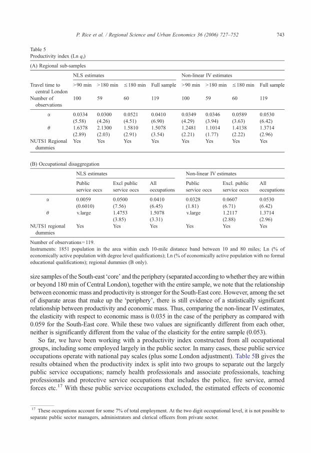
Table 5Productivity index (Ln qi)
(A) Regional sub-samples
NLS estimates Non-linear IV estimates
Travel time tocentral London
>90 min >180 min ≤180 min Full sample >90 min >180 min ≤180 min Full sample
Number ofobservations
100 59 60 119 100 59 60 119
α 0.0334(5.58)
0.0300(4.26)
0.0521(4.51)
0.0410(6.90)
0.0349(4.29)
0.0346(3.94)
0.0589(3.63)
0.0530(6.42)
θ 1.6378(2.89)
2.1300(2.03)
1.5810(2.91)
1.5078(3.54)
1.2481(2.21)
1.1014(1.77)
1.4138(2.22)
1.3714(2.96)
NUTS1 Regionaldummies
Yes Yes Yes Yes Yes Yes Yes Yes
(B) Occupational disaggregation
NLS estimates Non-linear IV estimates
Publicservice occs
Excl publicservice occs
Alloccupations
Publicservice occs
Excl. publicservice occs
Alloccupations
α 0.0059(0.6010)
0.0500(7.56)
0.0410(6.45)
0.0328(1.81)
0.0607(6.71)
0.0530(6.42)
θ v.large 1.4753(3.85)
1.5078(3.31)
v.large 1.2117(2.88)
1.3714(2.96)
NUTS1 regionaldummies
Yes Yes Yes Yes Yes Yes
Number of observations=119.Instruments: 1851 population in the area within each 10-mile distance band between 10 and 80 miles; Ln (% ofeconomically active population with degree level qualifications); Ln (% of economically active population with no formaleducational qualifications); regional dummies (B only).
743P. Rice et al. / Regional Science and Urban Economics 36 (2006) 727–752
size samples of the South-east ‘core’ and the periphery (separated according towhether they arewithinor beyond 180 min of Central London), together with the entire sample, we note that the relationshipbetween economic mass and productivity is stronger for the South-East core. However, among the setof disparate areas that make up the ‘periphery’, there is still evidence of a statistically significantrelationship between productivity and economic mass. Thus, comparing the non-linear IVestimates,the elasticity with respect to economic mass is 0.035 in the case of the periphery as compared with0.059 for the South-East core. While these two values are significantly different from each other,neither is significantly different from the value of the elasticity for the entire sample (0.053).
So far, we have been working with a productivity index constructed from all occupationalgroups, including some employed largely in the public sector. In many cases, these public serviceoccupations operate with national pay scales (plus some London adjustment). Table 5B gives theresults obtained when the productivity index is split into two groups to separate out the largelypublic service occupations; namely health professionals and associate professionals, teachingprofessionals and protective service occupations that includes the police, fire service, armedforces etc.17 With these public service occupations excluded, the estimated effects of economic
17 These occupations account for some 7% of total employment. At the two digit occupational level, it is not possible toseparate public sector managers, administrators and clerical officers from private sector.
744 P. Rice et al. / Regional Science and Urban Economics 36 (2006) 727–752
mass on the productivity index for the remaining set of occupations are greater. The estimatedelasticity is larger, while the spatial scale parameter is somewhat smaller indicating that thecontribution of population declines less rapidly with travel time. As one might expect, the effectsof economic mass on the productivity index for the public service group are much less welldetermined than for the full set of occupations. Convergence is achieved only with the spatialscale parameter set very large so that only population in the immediate vicinity (within 30 mindriving time) impacts on productivity, and even in this case, the estimated elasticity (the parameterα) is not well-determined. Results from splitting the sample this way are therefore as would beexpected, and increase somewhat the magnitude of effects for non-public service occupations.
6. Quantification: how large are the effects?
Having established that proximity to economic mass has statistically significant productivityeffects, we now turn to its quantitative importance. We base our discussion around the non-linearinstrumental variable estimates with regional dummies (Table 4, panel B), although similar effectscome from the separate time bands (Table 4, panel A).
First, how important is proximity in the relationship? We take as the central estimate of θ avalue of 1.37 (Table 4, panel B). This means that moving a mass of population 30 min furtheraway reduces its impact on productivity by three-quarters (exp(−1.37)=0.24). Thus, a person ofworking age between 60–70 min away has just 24% of the impact on productivity compared toan individual 30–40 min away. An individual 90–100 min away has 6% of the effect. A linear(rather than exponential) specification of the time weights is reported in appendix Table A2. Inthis case, an individual 60–70 min away has 40% of the effect of an individual 30–40 min away,and effects go to zero beyond 80 min. These are both quite steep rates of spatial decay, but areconsistent with studies in the literature. For example Rosenthal and Strange (2003) find that thepositive effect of established firms on entry of new firms in the same industry falls off sharplybetween 1 and 5 miles. Andersson, Quigley, and Wilhelmson (2004) identify productivityspillovers from university researchers, and find that half the total productivity gain accrueswithin 20 km.
The coefficient α is the elasticity of productivity with respect to distance-weighted spatial massand its estimated value is 0.053 (Table 4, lower panel). Quantitatively, an elasticity of 0.05 meansthat doubling the spatial mass that an area accesses increases its productivity by 3.5% (=20.05−1).This estimate is at the lower end of the range of estimates typically found in the literature. This isreviewed by Rosenthal and Strange (2004) who report a consensus view that ‘doubling city sizeseems to increase productivity by an amount that ranges from roughly 3–8%’.
An alternative approach to assessing the quantitative importance of access to economic mass indetermining productivity is to consider how much spatial variation in UK productivity isattributable to variation in economic mass and how much to variation in other factors. Table 6provides a decomposition of the variance of the (Ln) productivity index into the various sourcesusing the IVestimates of the non-linear spatial decay model as reported in Table 4 (lower half).18
Taking the sample as a whole, some 35% of the variance in (Ln) productivity is directlyattributable to variance in economic mass, as compared with the 43% that is due to variance in the
18 Given the spatial decay model specified in Eq. (4), the productivity index for area i may be decomposed as the sum ofthree components: economic mass mi ¼ a ln½Pb pbiexpðh ðtb−30Þ=30Þ�; qualifications and region specific factors edi ¼b0 þ
Pj bjxji; the residual ui. It follows that var(qi)=var(mi)+var(edi)+var(ui)+2cov(ui, edi)+2cov(mi, edi)+2cov(mi, ui).
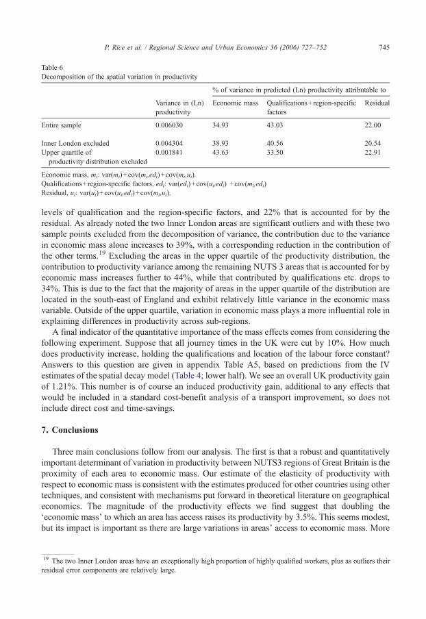
Table 6Decomposition of the spatial variation in productivity
% of variance in predicted (Ln) productivity attributable to
Variance in (Ln)productivity
Economic mass Qualifications+region-specificfactors
Residual
Entire sample 0.006030 34.93 43.03 22.00
Inner London excluded 0.004304 38.93 40.56 20.54Upper quartile of
productivity distribution excluded0.001841 43.63 33.50 22.91
Economic mass, mi: var(mi)+cov(mi,edi)+cov(mi,ui).Qualifications+region-specific factors, edi: var(edi)+cov(ui,edi) +cov(mi,edi)Residual, ui: var(ui)+cov(ui,edi)+cov(mi,ui).
745P. Rice et al. / Regional Science and Urban Economics 36 (2006) 727–752
levels of qualification and the region-specific factors, and 22% that is accounted for by theresidual. As already noted the two Inner London areas are significant outliers and with these twosample points excluded from the decomposition of variance, the contribution due to the variancein economic mass alone increases to 39%, with a corresponding reduction in the contribution ofthe other terms.19 Excluding the areas in the upper quartile of the productivity distribution, thecontribution to productivity variance among the remaining NUTS 3 areas that is accounted for byeconomic mass increases further to 44%, while that contributed by qualifications etc. drops to34%. This is due to the fact that the majority of areas in the upper quartile of the distribution arelocated in the south-east of England and exhibit relatively little variance in the economic massvariable. Outside of the upper quartile, variation in economic mass plays a more influential role inexplaining differences in productivity across sub-regions.
A final indicator of the quantitative importance of the mass effects comes from considering thefollowing experiment. Suppose that all journey times in the UK were cut by 10%. How muchdoes productivity increase, holding the qualifications and location of the labour force constant?Answers to this question are given in appendix Table A5, based on predictions from the IVestimates of the spatial decay model (Table 4; lower half). We see an overall UK productivity gainof 1.21%. This number is of course an induced productivity gain, additional to any effects thatwould be included in a standard cost-benefit analysis of a transport improvement, so does notinclude direct cost and time-savings.
7. Conclusions
Three main conclusions follow from our analysis. The first is that a robust and quantitativelyimportant determinant of variation in productivity between NUTS3 regions of Great Britain is theproximity of each area to economic mass. Our estimate of the elasticity of productivity withrespect to economic mass is consistent with the estimates produced for other countries using othertechniques, and consistent with mechanisms put forward in theoretical literature on geographicaleconomics. The magnitude of the productivity effects we find suggest that doubling the‘economic mass’ to which an area has access raises its productivity by 3.5%. This seems modest,but its impact is important as there are large variations in areas' access to economic mass. More
19 The two Inner London areas have an exceptionally high proportion of highly qualified workers, plus as outliers theirresidual error components are relatively large.
746 P. Rice et al. / Regional Science and Urban Economics 36 (2006) 727–752
than one third of the productivity variation between areas is due to variation in their access toeconomic mass, the effect being more important for areas in the lower half of the productivitydistribution.
The second is that our measure of economic mass gives economically meaningful measures ofthe role of proximity. For our central estimates, bringing population from 60 min driving-timeaway to 30 min away increases its impact on productivity by a factor of four. Consequently, thecounterfactual experiments of cutting all driving times in GB by 10% would raise productivity by1.2%, and twice this amount for areas whose access to large population mass is increased themost.
Finally, our productivity measure is based on a decomposition of earnings into a productivityeffect and an occupational composition effect. The occupational composition index captures theextent to which an area's employment is in occupations that are (relative to the average for GB asa whole) more or less well paid. The occupational composition index is positively correlated withproductivity, so regions with high productivity also tend to have good employment structures.However, we find no evidence of a systematic relationship between occupational composition andproximity to economic mass. This finding is consistent with the theory we outlined which–in itssimplest form–offers predictions about productivity, but not about the spatial structure ofoccupations.
Acknowledgement
Thanks to anonymous referees, Gilles Duranton, Henry Overman, Steven Redding and theparticipants in the conference “Understanding Productivity Differences” (Sardinia, June 2004) fortheir valuable comments and to the Evidence Based Policy Fund (UK Treasury, Office of theDeputy Prime Minister, Department of Trade and Industry) for financial support.
Appendix A. Decompositions
wik and li
k are wage and employment in occupation k and area i.Total employment in area i, Li=Σkli
k.Share of occupation k in employment in area i, λi
k= lik /Li.
Proportion of entire population in occupation k, λk=Σilik /ΣiLi.
Average wage in occupation k, w k=Σilikwi
k /ΣiLik, so w kλk=Σili
kwik /ΣiLi.
Average wage in area i ei=Σklikwi
k /Σklik=Σkλi
kwik.
Decomposition, for each area i:
ei ¼ Rkwki k
ki ¼ Rkwi
kk¯k þ Rk w
kkki þ Rkðwki −w
kÞðkki −k¯kÞ−Rk w
kk¯kor;
ei ¼ qi þ ci þ ri:
Appendix B. Data appendix
All data is at the level of the 126 NUTS 3 areas of Great Britain. To achieve a consistent dataset the following NUTS 3 areas are aggregated: East Cumbria and West Cumbria; South and WestDerbyshire and East Derbyshire; North Nottinghamshire and South Nottinghamshire; Isle of
747P. Rice et al. / Regional Science and Urban Economics 36 (2006) 727–752
Anglesey and Gwynedd; Caithness, Sutherland and Ross and Cromarty, Inverness and Nairn andMoray, Badenoch and Strathspey, Lochaber, Sky, Lochalsh and Argyll and the Islands. TheWestern Isles, Orkney Islands and Shetland Islands are excluded from the sample. Unlessotherwise stated, the data relate to the period 1998 to 2001, and the 4 years of data are averaged toremove short-run volatility.
GVA per (employee) hour worked (gi): Estimates of workplace-based gross value added atbasic prices are from the Office of National Statistics (2003). ONS estimates of GVA arecomputed using the income approach. Estimates of the main components of income – wages andsalaries for employees, self-employment income and gross trading profits – based on the locationof the workplace are derived from a range of sources including the Annual Business Inquiry, NewEarnings Survey and the Inland Revenue Survey of Personal Income. The remaining componentssuch as rental income are apportioned to a given area using a wages and salaries indicator. Forfurther details see Office of National Statistics (2003).
Total hours worked by employees is computed from data on the numbers of full-timeemployees and of part-time employees and the average weekly hours worked by each group takenfrom the Annual Business Inquiry.
Average hourly earnings (ei): Estimates of the average hourly earnings of all full-timeemployees whose pay was not affected by absence at the NUTS 3 level based on thelocation of workplace are taken from the New Earnings Surveys for the appropriateyears.
Productivity index (qi=Σkwik λk): Weighted sum of the average earnings of each occupational
group in area i, with weights equal to the share of the occupational group in total GB employment.Data on average hourly earnings of full-time employees at the level of the occupational majorgroup and at the two digit occupational level from the New Earnings Survey. The weights arecomputed from data on the share of 2-digit occupations in total GB employment from the LabourForce Survey 2001.
Composition index (ci=Σkwkλi
k): Weighted sum of the shares of each occupational majorgroup in employment in area i, with weights equal to the GB average earnings of theoccupational major group. Estimates of occupational shares in employment are derived from theLabour Force Survey for the appropriate years. Labour Force Survey data is residence-based,rather than workplace based, and this, coupled with the fact that the data is available only for themajor occupational groups, limits comparability with the productivity index. Weights arecomputed from data on the GB average hourly earnings by major occupational group from theNew Earnings Survey.
Population variables: Mid-year estimates of the total number of persons of working age (16 to65 years) resident in area i from Office of National Statistics.
Education variables: Proportion of economically active population resident in area i at each ofthe following qualification levels:
level 4 or higher: first and higher degree; nursing and teaching qualification;level 3: A-level; GNVQ Higher level, Advanced Certificate of Vocational Education;level 2: GCSE qualifications at grade or higher, GNVQ Intermediate level;level 1: GCSE qualifications below grade C, GNVQ Foundation level; trade apprenticeships;
no formal qualifications.
Data from the Labour Force Surveys, averaged for years 1999 to 2001.Travel times: Driving times between the population centres of NUTS 3 areas, are estimatedusing Microsoft Autoroute 2002. The Microsoft Autoroute software computes the estimateddriving time between two locations on the basis of the most efficient route given the road network
748 P. Rice et al. / Regional Science and Urban Economics 36 (2006) 727–752
in 2002, and allowing for different average speeds of travel depending on the type of road. Ingeneral the average speeds are set at the upper limit for road type, namely 70 mph for motorways,60 mph for other highways; 40 mph for major roads, 30 mph for minor roads and 18 mph forstreets within urban areas.
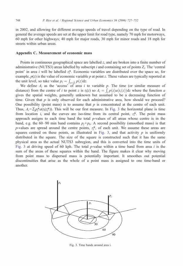
Appendix C. Measurement of economic mass
Points in continuous geographical space are labelled z, and are broken into a finite number ofadministrative (NUTS3) areas labelled by subscript i and containing set of points Zi. The ‘centralpoint’ in area i will be labelled zi⁎. Economic variables are distributed over the space so, forexample, p(z) is the value of economic variable p at point z. These values are typically reported atthe unit level, so take value pi ¼
RzaZi
pðzÞdz.We define Ai as the ‘access’ of area i to variable p. The time (or similar measure of
distance) from the centre of i to point z is ti(z) so Ai ¼Rz pðzÞaðtiðzÞÞdz where the function a
gives the spatial weights, generally unknown but assumed to be a decreasing function oftime. Given that p is only observed for each administrative area, how should we proceed?One possibility (point mass) is to assume that p is concentrated at the centre of each unit.Thus, Ai=Σjpj⁎a(ti(zj⁎)). This will be our first measure. In Fig. 3 the horizontal plane is timefrom location i, and the curves are iso-time from its central point, zi⁎. The point massapproach assigns to each time band the total p-values of all areas whose centre is in theband, e.g. the 60–90 min band contains pj+pk. A second possibility (smoothed mass) is thatp-values are spread around the centre points, zj⁎, of each unit. We assume these areas aresquares centred on these points, as illustrated in Fig. 3, and that activity p is uniformlydistributed in the square. The size of the square is constructed such that it has the samephysical area as the actual NUTS3 subregion, and this is converted into the time units ofFig. 3 at driving speed of 60 kph. The total p-value within a time band from area i is thesum of the areas of these squares within the band. The figure makes it clear why movingfrom point mass to dispersed mass is potentially important. It smoothes out potentialdiscontinuities that arise as the whole of a point mass is assigned to one time-band oranother.
Fig. 3. Time bands around area i.
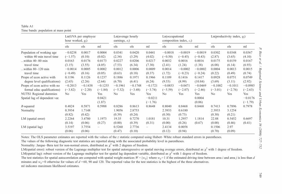
Table A1Time bands: population at mass point
Ln(GVA per employeehour worked, gi)
Ln(average hourlyearnings, ei)
Ln(occupationalcomposition index, ci)
Ln(productivity index, qi)
ols ols ml ols ols ml ols ols ml ols ols ml
Population of working agewithin 40 min travel time
−0.0238(−1.57)
0.0017(0.10)
0.0004(0.02)
0.0341(2.34)
0.0420(3.29)
0.0441(4.02)
−0.0018(−0.50)
−0.0019(−0.45)
−0.0019(−0.43)
0.0302(2.87)
0.0348(3.65)
0.0367(4.10)
…within 40–80 mintravel time
0.0163(3.15)
0.0176(3.55)
0.0173(4.05)
0.0227(7.53)
0.0206(6.34)
0.0217(7.30)
0.0032(2.41)
0.0016(1.24)
0.0016(1.38)
0.0175(6.08)
0.0159(6.14)
0.0167(6.93)
…within 80–120 mintravel time
−0.0014(−0.49)
0.0005(0.16)
0.0002(0.05)
0.0012(0.63)
0.0006(0.18)
0.0009(0.37)
0.0014(1.72)
−0.0002(−0.23)
−0.0002(−0.24)
0.0004(0.22)
0.0013(0.49)
0.0015(0.74)
Propn of econ active withdegree level qualifications)
0.1196(2.65)
0.1126(2.26)
0.1237(2.64)
0.1886(6.70)
0.1971(6.41)
0.1966(6.24)
0.1109(9.53)
0.1416(8.99)
0.1417(10.84)
0.0928(3.69)
0.0751(3.11)
0.0749(2.92)
Propn of econ active with noformal educ qualifications)
−0.2013(−3.82)
−0.1438(−2.20)
−0.1255(−1.84)
−0.1961(−5.32)
−0.1748(−3.48)
−0.1721(−3.74)
−0.0853(−5.59)
−0.0471(−2.07)
−0.0469(−2.46)
−0.1002(−3.01)
−0.1011(−2.76)
−0.0985(−2.63)
NUTS1 Regional dummies No Yes Yes No Yes Yes No Yes Yes No Yes YesSpatial lag of dependent var. 0.0421
(1.87)−0.0211(−1.76)
0.0004(0.06)
−0.0176(−1.79)
R-squared 0.4824 0.5871 0.5988 0.8286 0.8613 0.8648 0.8040 0.8468 0.8468 0.7413 0.7896 0.7978Normality 0.3934
(0.82)1.7148(0.42)
1.9056(0.39)
2.8753(0.24)
2.3933(0.30)
0.6180(0.73)
2.3933(0.30)
3.1254(0.21)
LM (spatial error) 2.2264(0.14)
3.4780(0.06)
1.1973(0.27)
19.35(0.00)
0.7270(0.39)
1.0181(0.31)
10.31(0.00)
1.2957(0.26)
1.1814(0.67)
22.88(0.00)
0.5452(0.46)
0.6697(0.41)
LM (spatial lag) 3.5197(0.06)
3.7554(0.06)
– 0.5260(0.47)
2.7736(0.10)
– 2.4134(0.12)
0.0058(0.94)
0.1506(0.70)
2.97(0.09)
Notes: The OLS parameter estimates are reported with the values of the z statistic computed using Hubert–White robust standard errors in parentheses.The values of the following diagnostic test statistics are reported along with the associated probability level in parentheses.Normality: Jarque–Bera test for non-normal errors, distributed as χ2 with 2 degrees of freedom.LM(spatial error): robust version of the Lagrange multiplier test for spatial autoregressive or spatial moving average errors, distributed as χ2 with 1 degree of freedom.LM(spatial lag): robust version of the Lagrange multiplier test for spatial lag dependent variable, distributed as χ2 with 1 degree of freedom.The test statistics for spatial autocorrelation are computed with spatial weight matrices W ={wij} where wij=1 if the estimated driving time between area i and area j is less than dminutes and wij=0 otherwise for values of d =60, 90 and 120. The reported value for the test statistics is the highest of the three alternatives.ml indicates maximum likelihood estimates.
749P.
Rice
etal.
/Regional
Scienceand
Urban
Econom
ics36
(2006)727–752
750 P. Rice et al. / Regional Science and Urban Economics 36 (2006) 727–752
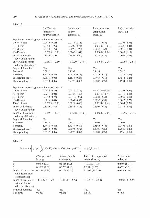
Table A2
Ln(GVA per(employee)hour worked, gi)
Ln(averagehourlyearnings, ei)
Ln(occupationalcompositionindex, ci)
Ln(productivityindex, qi)
Population of working age within travel time of
Up to 30 min 0.0059 (0.24) 0.0714 (2.78) 0.0039 (0.47) 0.0506 (2.76) 30–60 min 0.0198 (1.95) 0.0207 (2.74) −0.0030 (−1.04) 0.0206 (3.44) 60–90 min 0.0104 (1.76) 0.0096 (1.95) 0.0032 (1.63) 0.0056 (1.34) 90–120 min −0.0005 (−0.11) 0.0040 (1.04) −0.0000 (−0.00) 0.0039 (1.19) Ln(% with degreelevel qualifications
0.1139 (2.29) 0.1857 (5.50) 0.1379 (9.79) 0.0697 (2.74)Ln(% with no formaleduc. qualifications
−0.1378 (−2.10)
−0.1729 (−3.48) −0.0466 (−2.29) −0.0995 (−2.81)Regional dummies
Yes Yes Yes Yes R-squared 0.5812 0.8599 0.8488 0.7920 Normality 1.8189 (0.40) 1.9418 (0.38) 1.0385 (0.59) 0.9373 (0.63) LM (spatial error) 3.0053 (0.08) 1.1636 (0.28) 0.7467 (0.39) 1.4544 (0.23) LM (spatial lag) 3.5739 (0.06) 2.9120 (0.08) 0.0002 (0.99) 3.1984 (0.07)Population of working age within travel time of
Up to 40 min 0.0044 (0.23) 0.0489 (2.74) −0.0020 (−0.40) 0.0393 (3.36) 40–60 min 0.0271 (2.02) 0.0186 (1.80) −0.0015 (−0.41) 0.0179 (2.35) 60–80 min 0.0102 (0.79) 0.0111 (1.06) 0.0021 (0.61) 0.0080 (0.91) 80–100 min 0.0056 (0.43) 0.0061 (0.52) 0.0035 (0.97) 0.0022 (0.22) 100–120 min −0.0009 (−0.11) 0.0028 (0.40) −0.0014 (−0.67) 0.0044 (0.71) Ln (% with degreelevel qualifications
0.1149 (2.42) 0.1944 (5.81) 0.1397 (9.16) 0.0746 (2.91)Ln (% with no formaleduc. qualifications
−0.1354 (−1.97)
−0.1728 (−3.36) −0.0464 (−2.09) −0.0996 (−2.74)Regional dummies
Yes Yes Yes Yes R-squared 0.5837 0.8570 0.8496 0.7904 Normality 1.4478 (0.48) 1.4347 (0.49) 0.5565 (0.76) 0.7408 (0.69) LM (spatial error) 3.1594 (0.08) 0.9874 (0.32) 1.3188 (0.25) 1.2826 (0.26) LM (spatial lag) 3.6957 (0.05) 2.9022 (0.09) 0.0001 (0.99) 3.1966 (0.07)Table A3
lnyi ¼ alnXb
pbi1
60ð30−hðtb−30Þ þ absð30−hðtb−30ÞÞÞ
� �" #þXj
bjxji þ ei
GVA per workerhour, gI
Average hourlyearnings, ei
Index of occupationalcomposition, ci
Productivityindex, qi
α
0.0265 (2.77) 0.0415 (5.96) −0.0020 (−0.67) 0.0359 (6.34) θ 0.5000 (1.36) 0.5763 (4.93) 0.9998 (0.23) 0.6351 (3.55) Ln (% of econ activewith degree levelqualifications)
0.1191 (2.29)
0.2138 (5.65) 0.1399 (10.020) 0.0910 (3.04)Ln (% of econ activewith no formaleduc qualification)
−0.1287 (−1.65)
−0.1561 (−2.76) −0.0517 (−2.50) −0.0829 (−2.24)Regional dummies
Yes Yes Yes Yes R-squared 0.5520 0.8265 0.8449 0.7519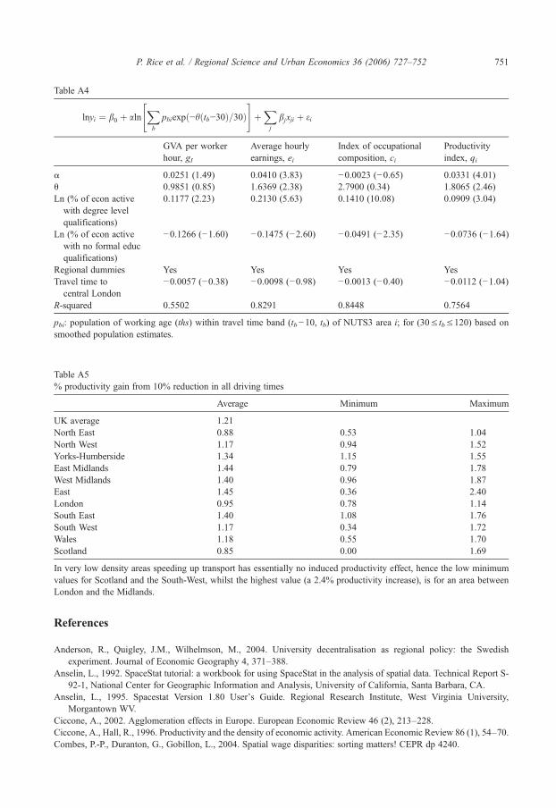
751P. Rice et al. / Regional Science and Urban Economics 36 (2006) 727–752
Table A4
lnyi ¼ b0 þ alnXb
pbiexpð−hðtb−30Þ=30Þ" #
þXj
bjxji þ ei
GVA per workerhour, gI
Average hourlyearnings, ei
Index of occupationalcomposition, ci
Productivityindex, qi
α
0.0251 (1.49) 0.0410 (3.83) −0.0023 (−0.65) 0.0331 (4.01) θ 0.9851 (0.85) 1.6369 (2.38) 2.7900 (0.34) 1.8065 (2.46) Ln (% of econ activewith degree levelqualifications)
0.1177 (2.23)
0.2130 (5.63) 0.1410 (10.08) 0.0909 (3.04)Ln (% of econ activewith no formal educqualifications)
−0.1266 (−1.60)
−0.1475 (−2.60) −0.0491 (−2.35) −0.0736 (−1.64)Regional dummies
Yes Yes Yes Yes Travel time tocentral London
−0.0057 (−0.38) −0.0098 (−0.98) −0.0013 (−0.40) −0.0112 (−1.04)R-squared
0.5502 0.8291 0.8448 0.7564pbi: population of working age (ths) within travel time band (tb−10, tb) of NUTS3 area i; for (30≤ tb≤120) based onsmoothed population estimates.
Table A5% productivity gain from 10% reduction in all driving times
Average
Minimum MaximumUK average
1.21 North East 0.88 0.53 1.04 North West 1.17 0.94 1.52 Yorks-Humberside 1.34 1.15 1.55 East Midlands 1.44 0.79 1.78 West Midlands 1.40 0.96 1.87 East 1.45 0.36 2.40 London 0.95 0.78 1.14 South East 1.40 1.08 1.76 South West 1.17 0.34 1.72 Wales 1.18 0.55 1.70 Scotland 0.85 0.00 1.69In very low density areas speeding up transport has essentially no induced productivity effect, hence the low minimumvalues for Scotland and the South-West, whilst the highest value (a 2.4% productivity increase), is for an area betweenLondon and the Midlands.
References
Anderson, R., Quigley, J.M., Wilhelmson, M., 2004. University decentralisation as regional policy: the Swedishexperiment. Journal of Economic Geography 4, 371–388.
Anselin, L., 1992. SpaceStat tutorial: a workbook for using SpaceStat in the analysis of spatial data. Technical Report S-92-1, National Center for Geographic Information and Analysis, University of California, Santa Barbara, CA.
Anselin, L., 1995. Spacestat Version 1.80 User's Guide. Regional Research Institute, West Virginia University,Morgantown WV.
Ciccone, A., 2002. Agglomeration effects in Europe. European Economic Review 46 (2), 213–228.Ciccone, A., Hall, R., 1996. Productivity and the density of economic activity. American Economic Review 86 (1), 54–70.Combes, P.-P., Duranton, G., Gobillon, L., 2004. Spatial wage disparities: sorting matters! CEPR dp 4240.
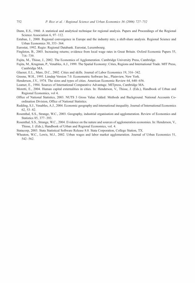
752 P. Rice et al. / Regional Science and Urban Economics 36 (2006) 727–752
Dunn, E.S., 1960. A statistical and analytical technique for regional analysis. Papers and Proceedings of the RegionalScience Association 6, 97–112.
Estaban, J., 2000. Regional convergence in Europe and the industry mix; a shift-share analysis. Regional Science andUrban Economics 30, 353–364.
Eurostat, 1992. Regio: Regional Databank. Eurostat, Luxembourg.Fingleton, B., 2003. Increasing returns; evidence from local wage rates in Great Britain. Oxford Economic Papers 55,
716–739.Fujita, M., Thisse, J., 2002. The Economics of Agglomeration. Cambridge University Press, Cambridge.Fujita, M., Krugman, P., Venables, A.J., 1999. The Spatial Economy: Cities, Regions and International Trade. MIT Press,
Cambridge MA.Glaeser, E.L., Mare, D.C., 2002. Cities and skills. Journal of Labor Economics 19, 316–342.Greene, W.H., 1995. Limdep Version 7.0. Econometric Software Inc., Plainview, New York.Henderson, J.V., 1974. The sizes and types of cities. American Economic Review 64, 640–656.Leamer, E., 1984. Sources of International Comparative Advantage. MITpress, Cambridge MA.Moretti, E., 2004. Human capital externalities in cities. In: Henderson, V., Thisse, J. (Eds.), Handbook of Urban and
Regional Economics, vol 4.Office of National Statistics, 2003. NUTS 3 Gross Value Added: Methods and Background. National Accounts Co-
ordination Division, Office of National Statistics.Redding, S.J., Venables, A.J., 2004. Economic geography and international inequality. Journal of International Economics
62, 53–82.Rosenthal, S.S., Strange, W.C., 2003. Geography, industrial organisation and agglomeration. Review of Economics and
Statistics 85, 377–393.Rosenthal, S.S., Strange, W.C., 2004. Evidence on the nature and sources of agglomeration economies. In: Henderson, V.,
Thisse, J. (Eds.), Handbook of Urban and Regional Economics, vol. 4.Statacorp, 2003. Stata Statistical Software Release 8.0. Stata Corporation, College Station, TX.Wheaton, W.C., Lewis, M.J., 2002. Urban wages and labor market agglomeration. Journal of Urban Economics 51,
542–562.