Université Libre de Bruxelles IT4BI Masters Program

Advanced Databases Course

2013 – 2014

SPATIAL DATABASES IN SQL SERVER 2008

Presented by: Andrés Zamora Rizkallah Touma

1

Table of Contents

Objective ............................................................................................................................................... 2

Introduction .......................................................................................................................................... 3

Spatial Databases in SQL Server 2008 .............................................................................................. 5 Geometry Shapes ........................................................................................................................................... 5 Spatial Reference Systems ............................................................................................................................ 6 Data Types ..................................................................................................................................................... 7 Storage ............................................................................................................................................................ 8 Creating New Spatial Data ........................................................................................................................... 9

Well-Known Text (WKT): ....................................................................................................................... 10 Well-Known Binary (WKB): .................................................................................................................... 10 Geography Markup Language (GML): ..................................................................................................... 10

Visualizing Spatial Data ............................................................................................................................. 12 Query Support ............................................................................................................................................. 13

Getting attributes of spatial data instances................................................................................................ 13 Relations between two spatial data instances ........................................................................................... 13 Spatial indices ........................................................................................................................................... 14

Comparison .................................................................................................................................................. 14

Case Study .......................................................................................................................................... 17 Sample Data ................................................................................................................................................. 17

Data Source ............................................................................................................................................... 17 Importing data into SQL ........................................................................................................................... 17

Visualization Tools ...................................................................................................................................... 18 Query Implementation................................................................................................................................ 19

1. Unary Operations ............................................................................................................................. 19 2. Distance Calculation ........................................................................................................................ 20 3. Set Operations .................................................................................................................................. 21 4. Advanced Functions ......................................................................................................................... 27

Observations ................................................................................................................................................ 30 Visualization Limit .......................................................................................................................... 30 Filter vs. STIntersects ...................................................................................................................... 30 Projection affects .............................................................................................................................. 31

Conclusion .......................................................................................................................................... 32

Bibliography ....................................................................................................................................... 33

2

Objective

The objective of this project is to demonstrate in an easy and understandable manner how we can

implement and manipulate spatial databases in SQL Server 2008.

At first, we will have a general introduction about spatial databases, their main domains, their

shortcomings and their future developments. Afterwards, the report will explain in detail the features

available in SQL Server 2008 to support the implementation of spatial databases. The third chapter

will talk about a case study we used to illustrate the utility of spatial databases with those features

and problems we encountered during the implementation.

Finally, we will have a conclusion summarizing the ideas found in the overall report.

3

Introduction

Data is ubiquitous in every aspect of the world and its physical objects can be measured, positioned

and moved. For that reason, spatial databases are built as a solution to store, query, manipulate and

analyze data based on information related to space. This spatial data “can be defined as pieces of

information describing quantitative and/or qualitative properties that refer to space. Such properties

can be represented as attributes of a set of objects or as functions of the space locations” (Belussi,

Catania, Clementini, & Ferrari, 2007).

As other databases, spatial databases take advantage of the technology to solve problems and needs,

especially to be able to monitor and support decision-making. The wide range of current applications

that uses these spatial capabilities are related to applications for urban development, social networks,

mobile phones like Waze, war strategies, insurance, medical treatments, computer-aided design

(CAD), astronomy, climate, events, retail stores, agriculture, robotics, satellite images, among others.

Hence, the diversity of users and the extensive number of customers have made it necessary to

increasingly study and develop these kinds of databases.

Regarding the use of spatial databases, Shekhar et al. mention: “The Geographical Information

System (GIS) is the principal technology motivating interest in Spatial Database Management

Systems (SDBMSs). GIS provides a convenient mechanism for the analysis and visualization of

geographic data. Geographic data is spatial data whose underlying frame of reference is the earth’s

surface” (Shekar & Chawla, 2003). Thus, it gives an idea of its main purpose and why the most of

the SDBMSs are focused on supporting those functionalities.

On the other hand, nowadays applications integrate many functions from the machines where they

are operating, and one of those is fully related with spatial databases, the GPS. This service is

responsible to determine the device’s location on Earth; it provides information about latitude,

longitude and altitude, although not all of the devices offer the last one. Additionally, there are other

means to collect information including physical addresses positioned in maps, IP addresses, satellites

and digital images.

Furthermore, in the book Spatial Database Systems, Yeung & Hall describe the trends of the

SDBMSs as integration between systems, cross platform applications, user friendly interfaces and

applications evolving in order to be able to solve the changing user requirements with new

technological developments. So that, they mention two main topics, spatial database systems as a

service and location based services. On one hand, it is a service provided through telecommunication

networks (usually Internet) using a hosted computer, which is paid either by subscription or number

of transactions, this service is called also Spatial Web Service. Yeung and Hall highlight one of the

best benefits of this approach: “Potentially millions of users are able to access spatial information,

and obtain business or public services based on such information without special software or

training” (Yeung & Hall, 2007)

On the other hand, location based services are mainly provided by mobile applications that provide

localized and real-time business and information services. These applications tend to adapt to their

context in order to provide information related to specific places.

4

Examples of the usage of this kind of applications are for weather, maps, touristic information,

traffic, and bike rental availability, among others. So that, users know the environment where they

are and can plan beforehand. Comparing to the conventional GIS used by some people, LBS has to

manage hundreds or thousands of requests simultaneously. So that, “In order to maintain a high level

of service in a concurrent real-time user environment, LBS demand much more stringent technology

and performance standards than those required by conventional spatial database applications”.

Hence, LBS are based in seven main capabilities: High performance, scalability, reliability, open

architecture, geographic coverage, severity and ease of use. In the Figure 1, Yeung & Hall classify

the different applications and they possible relation with spatial databases.

In their book, Yeung & Hall also mention that the diversification of GIS have reached multiple areas

regarding public administration (health care, security, law, transport…) in order to monitor, control

and manage the information and support the decision-making. Moreover, people will continue to be

one of the main reasons of spatial databases development. Finally, they list the most recent research

trends in the topic: Spatial data acquisition and integration, Distributed and mobile computing,

Geographic representation, Interoperability of geographic information, Open formats and GML,

Geographic data infrastructures, Spatial data and society, Spatial query optimization, Use of

geometry in database queries, Incorporation of time varying data into spatial databases, Use of

spatial data on the web, Knowledge discovery and spatial data mining and Improvement of

geospatial interoperability between systems, data types and databases.

Figure 1. Retrieved from Yeung, A., & Hall, B. (2007). Spatial Database Systems, Design,

Implementation and Project Management. Dordrecht, The Netherlands: Springer. Page 493.

5

Spatial Databases in SQL Server 2008

SQL Server 2008 is one of the most widely used database management systems to manipulate

databases in general. It was chosen as the means to manipulate spatial databases in this report

because of the features it provides in support of spatial databases and its accessibility. In this chapter

we will discuss the main spatial features available in SQL Server 2008 and at the end of the chapter

we will compare it with some other popular spatial database management systems. But first, we will

describe two important ideas about spatial data that are necessary to understand the dynamics of

manipulating such data with SQL Server 2008.

Geometry Shapes

Defining different spatial features – whether on earth or in abstract – mainly relies on a few basic

geometry shapes that must be available in a DBMS with spatial-data support. These shapes are

defined as follows:

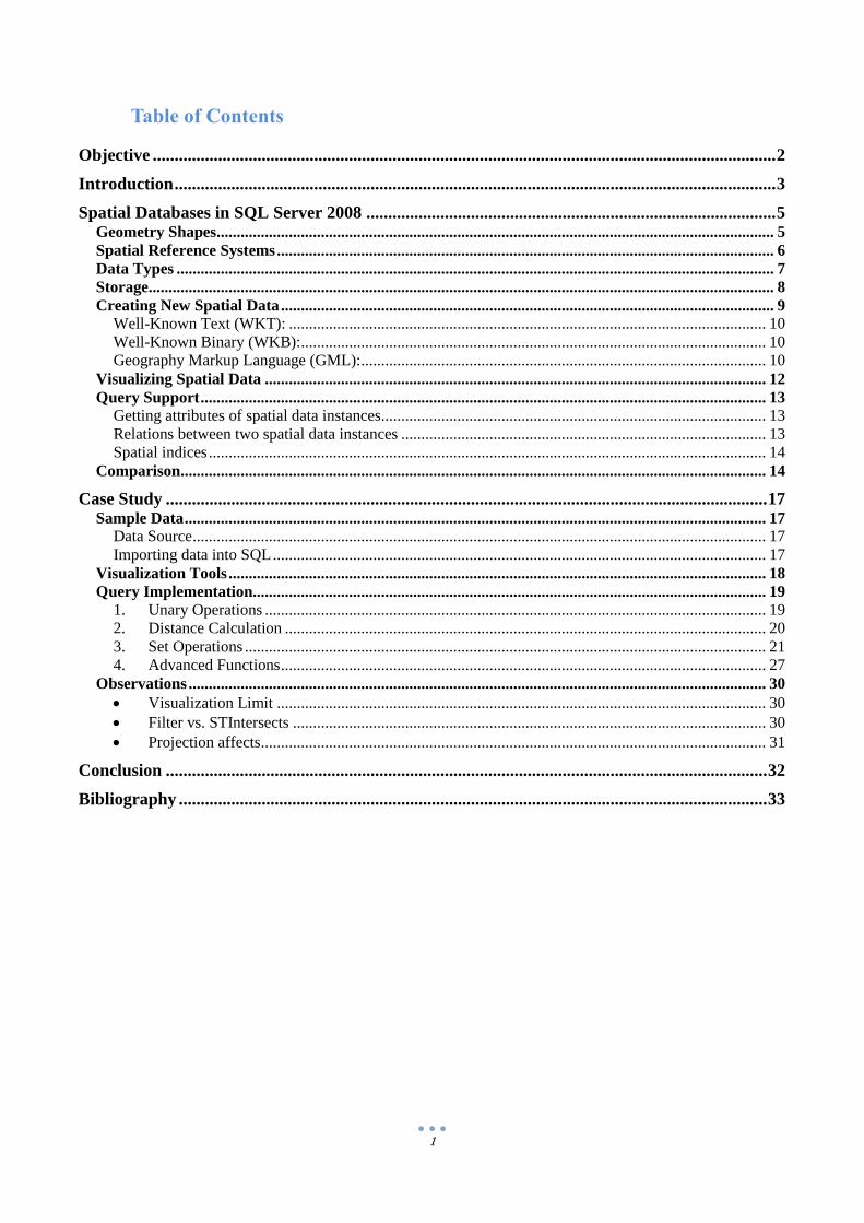
Point: a pair of coordinates that describes a specific location on a map (e.g. city, meeting

point, gift shop, …)

Figure 2. Retrieved from Aitchison, A. (2009). Beginning Spatial with SQL Server 2008. Apress. Page 5

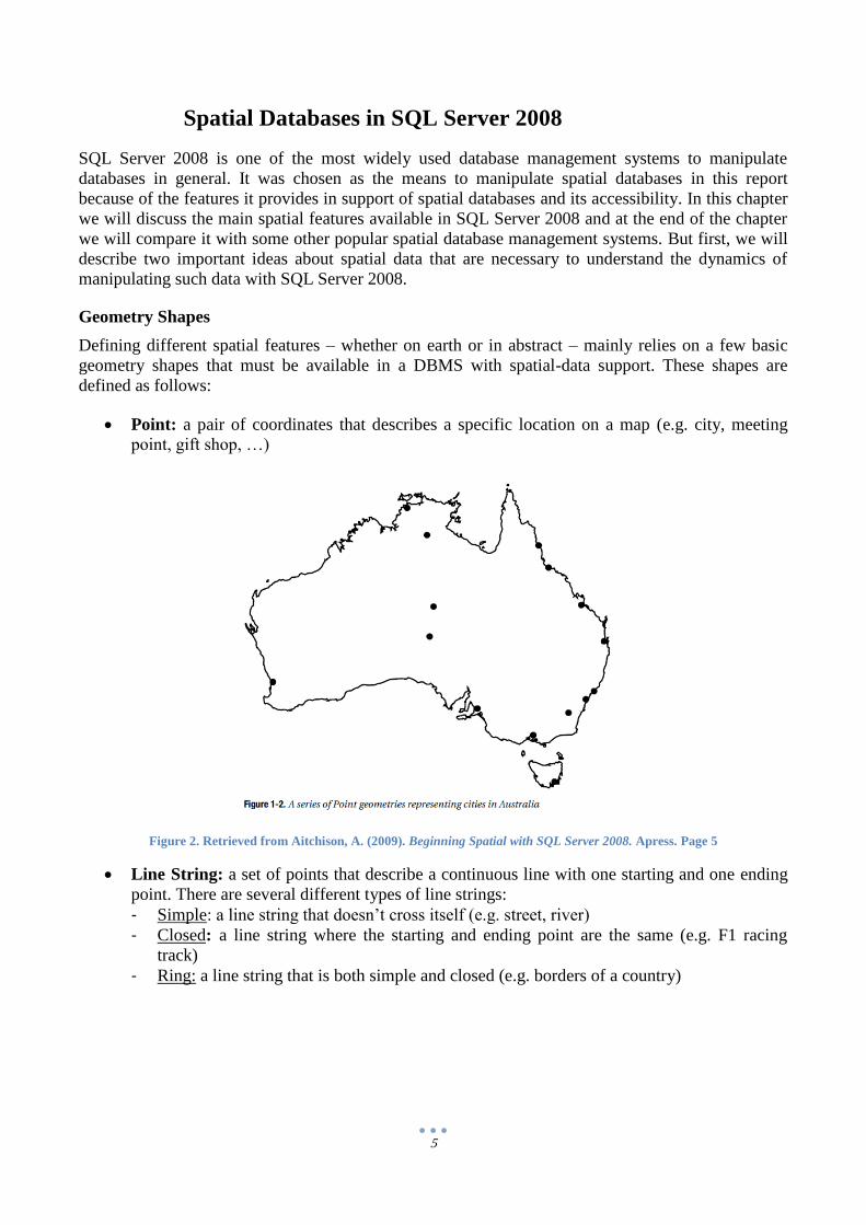
Line String: a set of points that describe a continuous line with one starting and one ending

point. There are several different types of line strings:

- Simple: a line string that doesn’t cross itself (e.g. street, river)

- Closed: a line string where the starting and ending point are the same (e.g. F1 racing

track)

- Ring: a line string that is both simple and closed (e.g. borders of a country)

6

Figure 3. Retrieved from Aitchison, A. (2009). Beginning Spatial with SQL Server 2008. Apress. Page 6

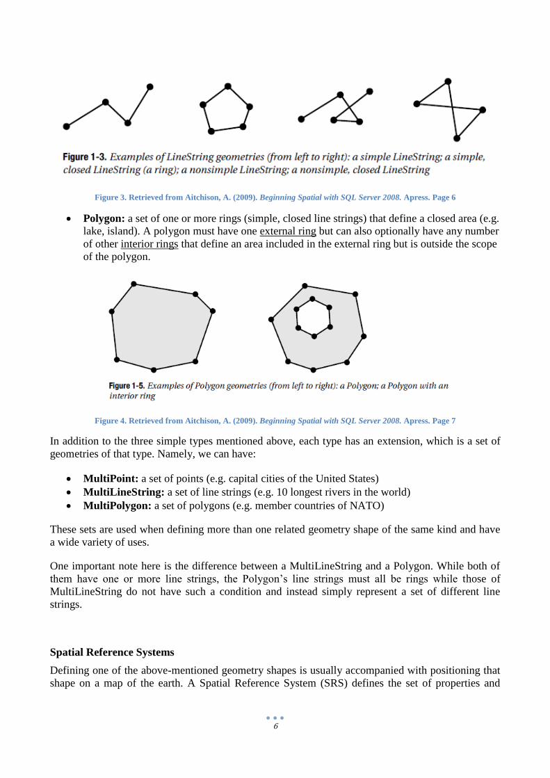
Polygon: a set of one or more rings (simple, closed line strings) that define a closed area (e.g.

lake, island). A polygon must have one external ring but can also optionally have any number

of other interior rings that define an area included in the external ring but is outside the scope

of the polygon.

Figure 4. Retrieved from Aitchison, A. (2009). Beginning Spatial with SQL Server 2008. Apress. Page 7

In addition to the three simple types mentioned above, each type has an extension, which is a set of

geometries of that type. Namely, we can have:

MultiPoint: a set of points (e.g. capital cities of the United States)

MultiLineString: a set of line strings (e.g. 10 longest rivers in the world)

MultiPolygon: a set of polygons (e.g. member countries of NATO)

These sets are used when defining more than one related geometry shape of the same kind and have

a wide variety of uses.

One important note here is the difference between a MultiLineString and a Polygon. While both of

them have one or more line strings, the Polygon’s line strings must all be rings while those of

MultiLineString do not have such a condition and instead simply represent a set of different line

strings.

Spatial Reference Systems

Defining one of the above-mentioned geometry shapes is usually accompanied with positioning that

shape on a map of the earth. A Spatial Reference System (SRS) defines the set of properties and

7

features that give meaning to the position of a shape on a map. An SRS usually consists of the

following:

Coordinate System: it is the set of axis that the coordinates should be mapped onto. There

are two main types:

- Geographic coordinate system: uses the latitude and longitude axis to map coordinates

onto a three-dimensional model of the earth

- Projected coordinate system: uses the linear (x) and (y) axis to map the coordinates onto a

projected two-dimensional model of the earth

Datum: a “datum” contains information about the shape and size of the earth as it is used to

map the coordinates on the coordinates system. It consists of the following:

- Reference Ellipsoid: since the shape of the earth cannot be accurately modeled in maps,

the reference ellipsoid describes the used 3D shape of the earth. It can be a perfect sphere

at times but it’s usually a different pre-defined ellipsoid.

- Reference Frame: defines the point with coordinates (0, 0) on the reference ellipsoid and

this point will be used as a reference for all other coordinates.

Prime Meridian: the axis from which the longitude coordinate will be measured (the most

commonly used prime meridian is that running through Greenwich, London)

Unit of Measure: determines the unit that the coordinates will be measured in. It depends on

the type of the coordinate system:

- Geographic coordinate systems use angular units (usually degree or radian)

- Projected coordinate systems use linear units (usually meters but can also be foot, yard,

mile for example)

Projection Parameters: in addition to all of the above, the projected coordinate system must

also have a set of projection parameters that defined the method used to project a 3D real-life

feature on a 2D model of the earth. The full set of parameters is explained in detail in

(Aitchison, 2009).

Instead of having to define all of the above parameters every time we want to define a spatial data

instance, SQL Server 2008 has an internal list of pre-defined SRS stored in the table

sys.spatial_reference_systems. All of the SRS in this table are regulated by the European Petroleum

Survey Group (EPSG) and each has its own unique SRID with which it can be referenced when

initializing spatial data.

Data Types

Exactly like number, varchar, float, int, etc, SQL Sever 2008 also has two main data types

specifically used to represent spatial data. These two types are called Geography and Geometry.

There are several similarities and differences between the two types in terms of usage, storage and

properties.

These similarities and differences are demonstrated in the below table:

Geography Geometry

Representation Both represent spatial data

Storage - Both store data internally as a string of bytes in the same format

- Both are variable-length data types (storage size depends on the

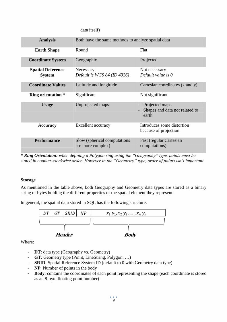
8

data itself)

Analysis Both have the same methods to analyze spatial data

Earth Shape Round Flat

Coordinate System Geographic Projected

Spatial Reference

System

Necessary

Default is WGS 84 (ID 4326)

Not necessary

Default value is 0

Coordinate Values Latitude and longitude Cartesian coordinates (x and y)

Ring orientation * Significant Not significant

Usage Unprojected maps - Projected maps

- Shapes and data not related to

earth

Accuracy Excellent accuracy Introduces some distortion

because of projection

Performance Slow (spherical computations

are more complex)

Fast (regular Cartesian

computations)

* Ring Orientation: when defining a Polygon ring using the “Geography” type, points must be

stated in counter-clockwise order. However in the “Geometry” type, order of points isn’t important.

Storage

As mentioned in the table above, both Geography and Geometry data types are stored as a binary

string of bytes holding the different properties of the spatial element they represent.

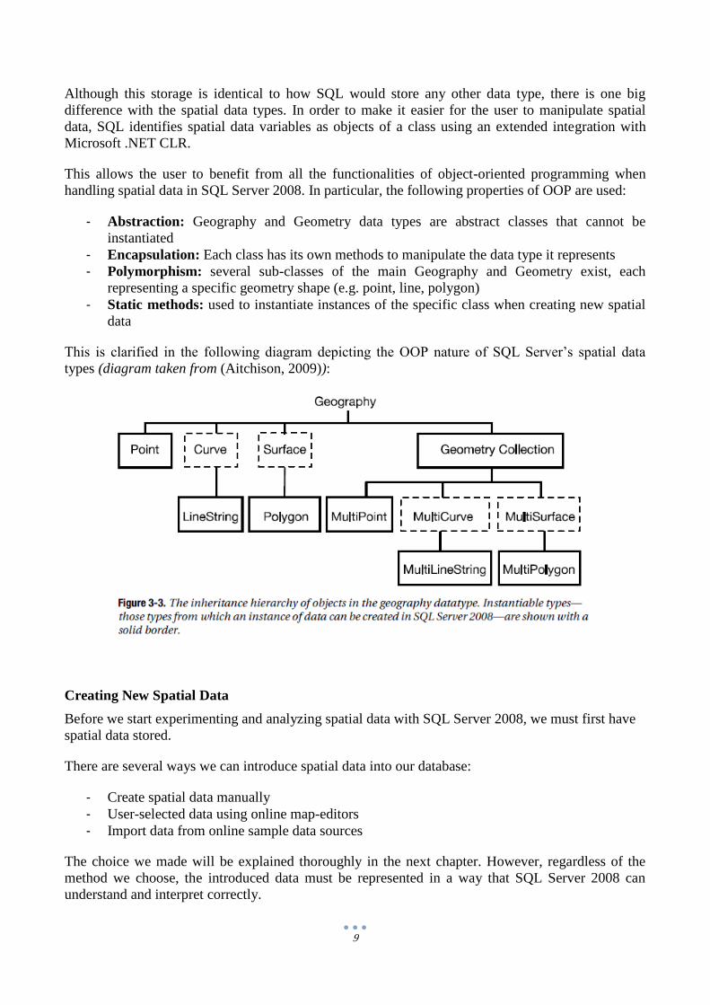
In general, the spatial data stored in SQL has the following structure:

Where:

- DT: data type (Geography vs. Geometry)

- GT: Geometry type (Point, LineString, Polygon, …)

- SRID: Spatial Reference System ID (default to 0 with Geometry data type)

- NP: Number of points in the body

- Body: contains the coordinates of each point representing the shape (each coordinate is stored

as an 8-byte floating point number)

Header Body

𝐷𝑇 𝐺𝑇 𝑆𝑅𝐼𝐷 𝑁𝑃 𝑥1 𝑦1, 𝑥2 𝑦2, … , 𝑥𝑛 𝑦𝑛

9

Although this storage is identical to how SQL would store any other data type, there is one big

difference with the spatial data types. In order to make it easier for the user to manipulate spatial

data, SQL identifies spatial data variables as objects of a class using an extended integration with

Microsoft .NET CLR.

This allows the user to benefit from all the functionalities of object-oriented programming when

handling spatial data in SQL Server 2008. In particular, the following properties of OOP are used:

- Abstraction: Geography and Geometry data types are abstract classes that cannot be

instantiated

- Encapsulation: Each class has its own methods to manipulate the data type it represents

- Polymorphism: several sub-classes of the main Geography and Geometry exist, each

representing a specific geometry shape (e.g. point, line, polygon)

- Static methods: used to instantiate instances of the specific class when creating new spatial

data

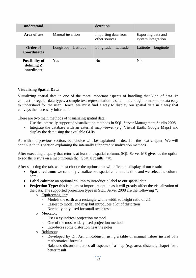
This is clarified in the following diagram depicting the OOP nature of SQL Server’s spatial data

types (diagram taken from (Aitchison, 2009)):

Creating New Spatial Data

Before we start experimenting and analyzing spatial data with SQL Server 2008, we must first have

spatial data stored.

There are several ways we can introduce spatial data into our database:

- Create spatial data manually

- User-selected data using online map-editors

- Import data from online sample data sources

The choice we made will be explained thoroughly in the next chapter. However, regardless of the

method we choose, the introduced data must be represented in a way that SQL Server 2008 can

understand and interpret correctly.

10

SQL Server 2008 has internal support for three different formats of spatial data representation. They

will be explained next.

Well-Known Text (WKT):

- Natural language text written in a pre-defined format

- SQL Server parses the text and creates the corresponding geometry shape

- Format:

o 𝑃𝑜𝑖𝑛𝑡 (𝑥 𝑦 𝑧): (z) is an optional third coordinate representing the depth of the point relative to

the surface of the earth

o 𝐿𝑖𝑛𝑒𝑆𝑡𝑟𝑖𝑛𝑔 (𝑥1 𝑦1, 𝑥2 𝑦2, … 𝑥𝑛 𝑦𝑛) o 𝑃𝑜𝑙𝑦𝑔𝑜𝑛 ((𝑥11 𝑦11, 𝑥12 𝑦12, … 𝑥11 𝑦11) (𝑥21 𝑦21, 𝑥22 𝑦22, … 𝑥21 𝑦21) (𝑥𝑚1 𝑦𝑚1, 𝑥𝑚2 𝑦𝑚2, … 𝑥𝑚1 𝑦𝑚1))

each LineString in the polygon definition must be a ring (i.e. must start and end at the same

point)

Well-Known Binary (WKB):

- Binary string of bytes in a pre-defined format

- Different from the binary format that SQL Server uses to internally store spatial data

- SQL Server converts this WKB to the format used in storage

- Format: o Point: [Type] = 1

o LineString: [Type] = 2

o Polygon: [Type] = 3

In the above formats, [ByteOrder] can be either 0 (big-endian) or 1(little-endian).

Geography Markup Language (GML):

- An XML-based markup language using pre-defined tags

- SQL Server can import the XML file and convert the XML data into the storage binary

representation

- Format: o Point:

11

o LineString:

o Polygon:

It should be noted that all of the formats explained above can be used to:

- Create both Geography and Geometry spatial data.

- Create sets of the above mentioned geometry shapes (i.e. MultiPoint, MultiLineString and

MultiPolygon).

The following table explains the main properties of each of them, the similarities and differences

between them and the main areas of use:

Well-Known Text

(WKT)

Well-Known Binary

(WKB)

Geography Markup

Language (GML)

Format Text-based Binary-based Text-based

Accuracy Low – due to rounding

errors

High – because of

binary representation

Low – due to rounding

errors

Processing Normal Fast Normal

Storage Normal Small Large

Easy to Very easy Hard – low error Very easy

12

understand detection

Area of use Manual insertion Importing data from

other sources

Exporting data and

system integration

Order of

Coordinates

Longitude – Latitude Longitude – Latitude Latitude – longitude

Possibility of

defining Z

coordinate

Yes No No

Visualizing Spatial Data

Visualizing spatial data in one of the more important aspects of handling that kind of data. In

contrast to regular data types, a simple text representation is often not enough to make the data easy

to understand for the user. Hence, we must find a way to display our spatial data in a way that

conveys the necessary information.

There are two main methods of visualizing spatial data:

- Use the internally supported visualization methods in SQL Server Management Studio 2008

- Integrate the database with an external map viewer (e.g. Virtual Earth, Google Maps) and

display the data using the available GUIs

As with the previous section, our choice will be explained in detail in the next chapter. We will

continue in this section explaining the internally supported visualization methods.

After executing a query that returns at least one spatial column, SQL Server MS gives us the option

to see the results on a map through the “Spatial results” tab.

After selecting the tab, we must choose the options that will affect the display of our result:

Spatial column: we can only visualize one spatial column at a time and we select the column

here

Label column: an optional column to introduce a label to our spatial data

Projection Type: this is the most important option as it will greatly affect the visualization of

the data. The supported projection types in SQL Server 2008 are the following *:

o Equirectangular:

- Models the earth as a rectangle with a width to height ratio of 2:1

- Easiest to model and map but introduces a lot of distortion

- Normally only used for small-scale tests

o Mercator:

- Uses a cylindrical projection method

- One of the most widely used projection methods

- Introduces some distortion near the poles

o Robinson:

- Developed by Dr. Arthur Robinson using a table of manual values instead of a

mathematical formula

- Balances distortion across all aspects of a map (e.g. area, distance, shape) for a

better result

13

o Bonne:

- All the parallels of latitude are constructed from the concentric arcs of a circle

- Usually introduces a lot of distortion when used for the map of the whole world

and hence it is mostly used for maps of smaller parts (e.g. continents or countries)

Please note that since the Geometry data type is already projected, this option is only

available when visualizing Geography data.

* More information about these projection types and illustrations of the differences between them is

mentioned in (Aitchison, 2009).

Query Support

After introducing the main spatial data types in SQL Server 2008, we will talk about how these data

types are in integrated into T-SQL language and what are the main features available to handle them

in a spatial-related manner.

Continuing with the object-oriented approach that SQL Server 2008 takes when is dealing with

spatial data, many attributes and functions are available to handle the defined spatial data in the same

way it is created.

Getting attributes of spatial data instances

The following attributes can be retrieved using specific “get” methods. Unless otherwise noted, all

methods are valid for both the Geography and Geometry data types:

Get type of geometry (point, lineString, …)

Get number of dimensions

Test the properties of a lineString (simple / closed / ring) (Geometry type only)

Get number of points in a geometry shape

Get coordinates of a point (x and y for Geometry, longitude and latitude for Geography)

Get start point and end point of a geometry shape

Get the centroid of a polygon (Geometry type only)

Get the envelope center of a polygon (Geography type only, takes into consideration the 3D

nature of the polygon)

Get length / area of a geometry shape

Get exterior ring / number of interior rings / a specific interior ring of a polygon

Relations between two spatial data instances

Another important aspect of support for spatial data is defining the relations between two spatial data

instances. SQL Server 2008 also has a number of functions to define the most used binary relations,

listed below:

Get the union / intersection / difference / symmetric difference of two geometry shapes (all

these relations are defined as set operations on the set of points of each geometry and return

the simplest shape possible containing the points that satisfy the relation)

Testing equality of two shapes (also points-wise)

Calculate distance between two geometry shapes (shortest direct path)

Testing if two geometry shapes intersect or are disjoint

14

Testing if two geometry shapes touch each other (two shapes “touch” each other if all of the

points they share lie on the boundary of both of them)

Testing if two polygons overlap

Testing the containment of one geometry shape in another

Spatial indices

As with other types of queries, spatial queries might need a very long time to execute. For examples,

testing a binary relation between two shapes might consume a long time depending on the

complexity of the shapes and the size of the spatial data set we have.

In order to enhance the performance, SQL Server 2008 uses a special type of indices called “spatial

indices”. A spatial index is implemented as a grid index with a structure similar to a B-Tree in

principle. It basically works in the following way:

- Divide the space of spatial data into (n) different cells

- Divide each cell into another (n) squares

- Repeat the above until we reach a pre-defines (h) number of levels (number of level in SQL is

set to h = 4 and cannot be changed)

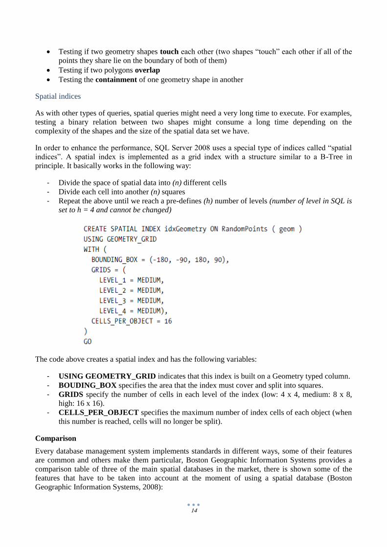
The code above creates a spatial index and has the following variables:

- USING GEOMETRY_GRID indicates that this index is built on a Geometry typed column.

- BOUDING_BOX specifies the area that the index must cover and split into squares.

- GRIDS specify the number of cells in each level of the index (low: 4 x 4, medium: 8 x 8,

high: 16 x 16).

- CELLS_PER_OBJECT specifies the maximum number of index cells of each object (when

this number is reached, cells will no longer be split).

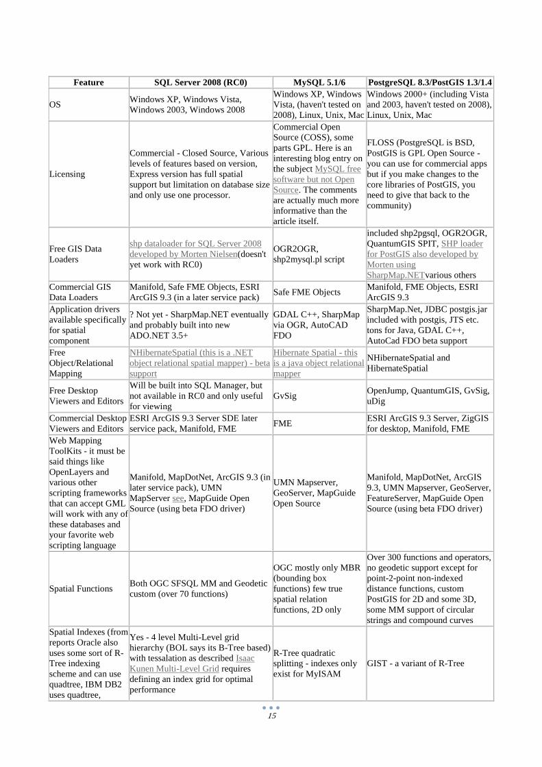
Comparison

Every database management system implements standards in different ways, some of their features

are common and others make them particular, Boston Geographic Information Systems provides a

comparison table of three of the main spatial databases in the market, there is shown some of the

features that have to be taken into account at the moment of using a spatial database (Boston

Geographic Information Systems, 2008):

15

Feature SQL Server 2008 (RC0) MySQL 5.1/6 PostgreSQL 8.3/PostGIS 1.3/1.4

OS Windows XP, Windows Vista,

Windows 2003, Windows 2008

Windows XP, Windows

Vista, (haven't tested on

2008), Linux, Unix, Mac

Windows 2000+ (including Vista

and 2003, haven't tested on 2008),

Linux, Unix, Mac

Licensing

Commercial - Closed Source, Various

levels of features based on version,

Express version has full spatial

support but limitation on database size

and only use one processor.

Commercial Open

Source (COSS), some

parts GPL. Here is an

interesting blog entry on

the subject MySQL free

software but not Open

Source. The comments

are actually much more

informative than the

article itself.

FLOSS (PostgreSQL is BSD,

PostGIS is GPL Open Source -

you can use for commercial apps

but if you make changes to the

core libraries of PostGIS, you

need to give that back to the

community)

Free GIS Data

Loaders

shp dataloader for SQL Server 2008

developed by Morten Nielsen(doesn't

yet work with RC0)

OGR2OGR,

shp2mysql.pl script

included shp2pgsql, OGR2OGR,

QuantumGIS SPIT, SHP loader

for PostGIS also developed by

Morten using

SharpMap.NETvarious others

Commercial GIS

Data Loaders

Manifold, Safe FME Objects, ESRI

ArcGIS 9.3 (in a later service pack) Safe FME Objects

Manifold, FME Objects, ESRI

ArcGIS 9.3

Application drivers

available specifically

for spatial

component

? Not yet - SharpMap.NET eventually

and probably built into new

ADO.NET 3.5+

GDAL C++, SharpMap

via OGR, AutoCAD

FDO

SharpMap.Net, JDBC postgis.jar

included with postgis, JTS etc.

tons for Java, GDAL C++,

AutoCad FDO beta support

Free

Object/Relational

Mapping

NHibernateSpatial (this is a .NET

object relational spatial mapper) - beta

support

Hibernate Spatial - this

is a java object relational

mapper

NHibernateSpatial and

HibernateSpatial

Free Desktop

Viewers and Editors

Will be built into SQL Manager, but

not available in RC0 and only useful

for viewing

GvSig OpenJump, QuantumGIS, GvSig,

uDig

Commercial Desktop

Viewers and Editors

ESRI ArcGIS 9.3 Server SDE later

service pack, Manifold, FME FME

ESRI ArcGIS 9.3 Server, ZigGIS

for desktop, Manifold, FME

Web Mapping

ToolKits - it must be

said things like

OpenLayers and

various other

scripting frameworks

that can accept GML

will work with any of

these databases and

your favorite web

scripting language

Manifold, MapDotNet, ArcGIS 9.3 (in

later service pack), UMN

MapServer see, MapGuide Open

Source (using beta FDO driver)

UMN Mapserver,

GeoServer, MapGuide

Open Source

Manifold, MapDotNet, ArcGIS

9.3, UMN Mapserver, GeoServer,

FeatureServer, MapGuide Open

Source (using beta FDO driver)

Spatial Functions Both OGC SFSQL MM and Geodetic

custom (over 70 functions)

OGC mostly only MBR

(bounding box

functions) few true

spatial relation

functions, 2D only

Over 300 functions and operators,

no geodetic support except for

point-2-point non-indexed

distance functions, custom

PostGIS for 2D and some 3D,

some MM support of circular

strings and compound curves

Spatial Indexes (from

reports Oracle also

uses some sort of R-

Tree indexing

scheme and can use

quadtree, IBM DB2

uses quadtree,

Yes - 4 level Multi-Level grid

hierarchy (BOL says its B-Tree based)

with tessalation as described Isaac

Kunen Multi-Level Grid requires

defining an index grid for optimal

performance

R-Tree quadratic

splitting - indexes only

exist for MyISAM

GIST - a variant of R-Tree

16

Spherical Voronoi

Tessalation, IBM

Informix uses R-

Tree. Note R-Tree

indexes are self-

tuning and do not

require grid setup

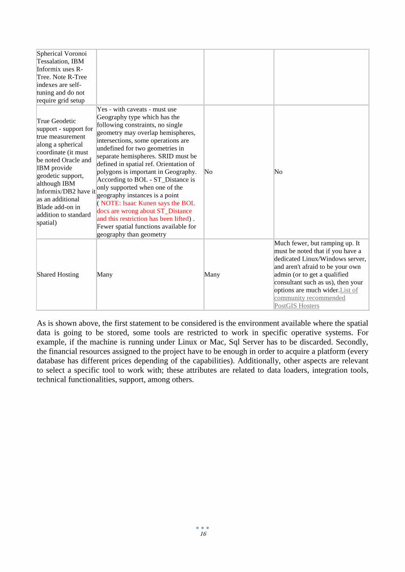
True Geodetic

support - support for

true measurement

along a spherical

coordinate (it must

be noted Oracle and

IBM provide

geodetic support,

although IBM

Informix/DB2 have it

as an additional

Blade add-on in

addition to standard

spatial)

Yes - with caveats - must use

Geography type which has the

following constraints, no single

geometry may overlap hemispheres,

intersections, some operations are

undefined for two geometries in

separate hemispheres. SRID must be

defined in spatial ref. Orientation of

polygons is important in Geography.

According to BOL - ST_Distance is

only supported when one of the

geography instances is a point

( NOTE: Isaac Kunen says the BOL

docs are wrong about ST_Distance

and this restriction has been lifted) .

Fewer spatial functions available for

geography than geometry

No No

Shared Hosting Many Many

Much fewer, but ramping up. It

must be noted that if you have a

dedicated Linux/Windows server,

and aren't afraid to be your own

admin (or to get a qualified

consultant such as us), then your

options are much wider.List of

community recommended

PostGIS Hosters

As is shown above, the first statement to be considered is the environment available where the spatial

data is going to be stored, some tools are restricted to work in specific operative systems. For

example, if the machine is running under Linux or Mac, Sql Server has to be discarded. Secondly,

the financial resources assigned to the project have to be enough in order to acquire a platform (every

database has different prices depending of the capabilities). Additionally, other aspects are relevant

to select a specific tool to work with; these attributes are related to data loaders, integration tools,

technical functionalities, support, among others.

17

Case Study

Sample Data

Before starting with our implementation, we will talk in a small section about the sample data we

collected and manipulated in the project.

In our case, we did not need data that was 100% accurate since we are only demonstrating the spatial

functionalities of SQL Server 2008. However, in real-world spatial applications, gathering spatial

data takes up a big part of the project because of the inaccuracy and limitations of most data sources

available on the web.

Data Source

We collected all of our sample data from VDS Technologies (http://www.vdstech.com/home.aspx).

They offer free spatial data for GIS and mapping purposes. We used the following data sets from

their World Map Data source:

- World Political Map: contains countries of the world as geometry polygons

- Coast Lines: contains the coastal lines of the world defined as line strings

- City Areas: contains major cities of the world described as polygons and not as points

- Airports: contains the major airports of the world (civilian / cargo / military) defined as

geometry points

- Railroads: contains the major railroads of the world defined as line strings

- Lakes: contains the major lakes of the world defined as polygons

All of the above data was coded in Shapefile format which is one of the most commonly used spatial

file formats. Each data source consists of three main files:

- .shp: this file contains the raw spatial data. It can only hold data of one kind (e.g. polygon,

point, line string)

- .shx: contains the spatial index of the .shp file. It has an entry for each shape in the

accompanying .shp file

- .dbf: contains additional non-spatial info for each shape in .shp file (e.g., name of country)

All of the data in the files represent Geometry shapes. The shapes were projected using the WGS

1984 Coordinate System on a scale 1:1,000,000.

Importing data into SQL

Importing the Shapefile data into SQL was done using the Shape2SQL tool

(http://sharpgis.net/page/SQL-Server-2008-Spatial-Tools.aspx). Shape2SQL is a popular free tool

built specifically to import Shapefiles into SQL Server 2008.

Importing is done on a file-by-file basis. The screenshot below demonstrates the simple interface of

Shape2SQL. Several options are given including the type of data (geometry / geography), creating a

spatial index, and the choice of attributes to include from the .shp file.

Once the correct options are chosen, the file is imported and a corresponding table is created in the

database.

18

Visualization Tools

As stated before, Geographical Information Systems (GIS) gives the possibility to manage, analyze

and present all types of geographical data. So that, GIS help users to visualize geographical data

through interactive actions, usually the topics are related to land, water, transportation,

geomarketing, urban planning, among others. Here, will be presented 4 of these GIS, each of those

with its differences.

ArcGIS

This GIS, as its website states, is a: “comprehensive system that allows people to collect, organize,

manage, analyze, communicate, and distribute geographic information. As the world's leading

platform for building and using geographic information systems (GIS), ArcGIS is used by people all

over the world to put geographic knowledge to work in government, business, science, education,

and media. ArcGIS enables geographic information to be published so it can be accessed and used by

anyone. The system is available everywhere using web browsers, mobile devices such as

smartphones, and desktop computers” (ESRI). Thus, throughout a robust variety of products, users

can create, share and use maps; create and manage geographic databases and make spatial analysis,

in diverse platforms (desktops, web, mobile).

Open Jump

Open Jump is a solution open source written in the Java programming language, developed and

maintained by volunteers. It can read and write shape (.shp) and simple GML files. And, as is stated

in its website “It has limited support for the display of images and good support for showing data

19

retrieved from WFS and WMS web-services. So you can use it as GIS Data Viewer. However, its

particular strength is the editing of geometry and attribute data” (Open Jump, 2011).

SQL Server Reporting Services 2008 (SSRS)

This tool, provided by Microsoft, is included in the SQL Server 2008. It is made to create and

manage customized reports. Reports can include tables, charts, maps, gauges, indicators, spark lines

and data bars and can be connected with different sources of data. To present the information to the

users, these reports can be showed locally or published to a server or SharePoint site (Microsoft).

SQL Server Management Studio 2008 (SSMS)

SSMS is an application developed by Microsoft for windows platforms. It gives the possibility to

access, manage, configure and administer SQL Server components (Microsoft). Combining the

capabilities for advanced and beginner users, it contains script editors for SQL queries and graphical

viewers to show spatial results, as well, managing tools for SQL Server Database Engine, Analysis

Services, Reporting Services, among others.

For this project, were checked different tools to store, manipulate and represent spatial data. Finally,

we decided to use SQL Server Management Studio due to the ease of acquiring the software and the

integration of components. The data was imported from shape files and stored in the SQL Server

database. Then, the queries were written in the SSMS and the spatial results shown in the same

program.

Query Implementation

After introducing all of the components necessary to implement spatial databases with SQL Server,

we will talk in this section about the different queries we used to test SQL Server spatial capabilities.

One function that will be used extensively throughout the examples here is MakeValid(). This

function checks if a geometry shape is defined correctly and if not, tries to make it valid (e.g., if a

polygon is defined with only 2 points, it converts it to a line string).

We needed to use this function because SQL Server 2008 allows the user to define geometry shapes

incorrectly but doesn’t allow the application of any methods on them. To our surprise, while

executing the tests we found that several instances of the sample data were defined incorrectly and

needed the use of MakeValid() before applying the actual method we wanted to test.

1. Unary Operations

Several unary operations are available on spatial data. We will test two of the most popular:

STLength: returns the length of a geometry (in case of a polygon, it returns the total length of

the line strings comprising the boundary of that polygon)

Example: Find the length of the borders of Belgium

Query:

SELECT WM.Geom.MakeValid().STLength()

FROM WorldMap WM

WHERE WM.NAME = 'Belgium'

20

STArea: returns the area contained within a geometry

Example: Select the top 10 largest countries of the European Union according to area

Query:

SELECT TOP 10 WM.NAME, WM.Geom.MakeValid().STArea()

FROM WorldMap WM

WHERE WM.NAME IN ('Austria', 'Belgium', 'Bulgaria', 'Croatia', 'Cyprus', 'Czech',

'Denmark', 'Estonia', 'Finland', 'France', 'Germany', 'Greece', 'Hungary', 'Ireland', 'Italy', 'Latvia',

'Lithuania', 'Luxembourg', 'Malta', 'Netherlands', 'Poland', 'Portugal', 'Romania', 'Slovakia', 'Slovenia',

'Spain', 'Sweden', 'United Kingdom')

ORDER BY WM.Geom.MakeValid().STArea() DESC

Note: the unit of measurement in the above examples is the same as the unit of coordinates (i.e., the

length of a lines string between (2, 2) and (5, 6) is 5 units, regardless of the actual unit of

measurement).

2. Distance Calculation

STDistance(): this function calculates the shortest distance between two shapes (e.g., if the

shapes were a point and a polygon, it would calculate the shortest distance from the point to the

polygon)

Example: List the 10 closest airports to Istanbul, Turkey

Query 1:

DECLARE @IstanbulCity GEOMETRY;

SELECT @IstanbulCity = CA.GEOM

FROM CITYAREAS CA

WHERE CA.NAME = 'ISTANBUL';

SELECT TOP 10 A.Name, A.GEOM.STAsText()

FROM AIRPORTS A

ORDER BY A.GEOM.MakeValid().STDistance(@IstanbulCity) ASC;

21

Query 2: As mentioned before, the cities in the sample data are represented as polygons and not

as points so as a variant, let us consider the same query but calculate the distance from the center

of Istanbul. This can be given by applying the STCentroid function:

DECLARE @IstanbulCenter GEOMETRY;

SELECT @IstanbulCenter = CA.GEOM.STCentroid()

FROM CITYAREAS CA

WHERE CA.NAME = 'ISTANBUL';

SELECT TOP 10 A.Name, A.GEOM.STAsText()

FROM AIRPORTS A

ORDER BY A.GEOM.MakeValid().STDistance(@IstanbulCenter) ASC;

3. Set Operations

To demonstrate how SQL Server supports set operations on spatial data, we will consider the

following cases:

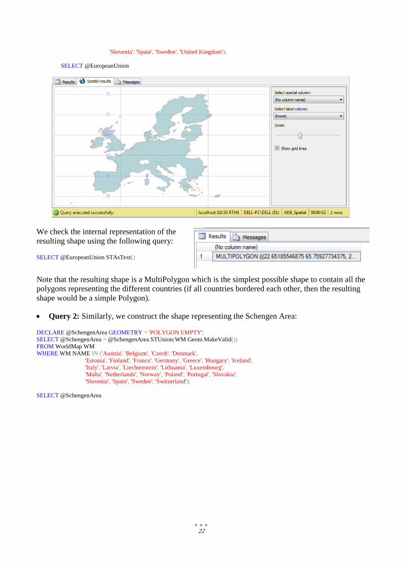
STUnion(): merges geometry shapes together and the result is the most simple type that can

contain all the shapes to be merged

Example: Construct the geometry shapes representing the European Union and the Schengen

Area

Query 1:

DECLARE @EuropeanUnion GEOMETRY = 'POLYGON EMPTY';

SELECT @EuropeanUnion = @EuropeanUnion.STUnion(WM.Geom.MakeValid())

FROM WorldMap WM

WHERE WM.NAME IN ('Austria', 'Belgium', 'Bulgaria', 'Croatia', 'Cyprus', 'Czech',

'Denmark', 'Estonia', 'Finland', 'France', 'Germany', 'Greece',

'Hungary', 'Ireland', 'Italy', 'Latvia', 'Lithuania', 'Luxembourg',

'Malta', 'Netherlands', 'Poland', 'Portugal', 'Romania', 'Slovakia',

22

'Slovenia', 'Spain', 'Sweden', 'United Kingdom');

SELECT @EuropeanUnion

We check the internal representation of the

resulting shape using the following query:

SELECT @EuropeanUnion.STAsText()

Note that the resulting shape is a MultiPolygon which is the simplest possible shape to contain all the

polygons representing the different countries (if all countries bordered each other, then the resulting

shape would be a simple Polygon).

Query 2: Similarly, we construct the shape representing the Schengen Area:

DECLARE @SchengenArea GEOMETRY = 'POLYGON EMPTY';

SELECT @SchengenArea = @SchengenArea.STUnion(WM.Geom.MakeValid())

FROM WorldMap WM

WHERE WM.NAME IN ('Austria', 'Belgium', 'Czech', 'Denmark',

'Estonia', 'Finland', 'France', 'Germany', 'Greece', 'Hungary', 'Iceland',

'Italy', 'Latvia', 'Liechtenstein', 'Lithuania', 'Luxembourg',

'Malta', 'Netherlands', 'Norway', 'Poland', 'Portugal', 'Slovakia',

'Slovenia', 'Spain', 'Sweden', 'Switzerland');

SELECT @SchengenArea

23

Checking the internal representation of

the Schengen Area shape would give

MultiPolygon for the same reasons as

above:

SELECT @SchengenArea.STAsText()

STDifference: returns the simplest shape representing the set difference of two shapes (all of the

shapes that exist in the first shape but not in the second)

Example: Give the countries that are in the Schengen Area but are not members of the European

Union

Query:

SELECT @SchengenArea.STDifference(@EuropeanUnion);

Note that the above map indeed shows the 4 countries satisfying the criteria (Norway, Iceland,

Liechtenstein and Switzerland)

24

STSymDifference: returns the simplest shape representing the symmetric difference of two

shapes (all of the shapes that are in either one of the shape but not in both)

Example: Give all the countries that are in either the EU or the Schengen Area but not in both

Query:

SELECT @SchengenArea.STSymDifference(@EuropeanUnion);

This map shows the countries contained in the first map plus the 6 EU countries that are not part of the

Schengen Area (Bulgaria, Croatia, Cyprus, Ireland, Romania and UK)

STIntersection: returns the simplest shape representing the intersection between two geometry

shapes (simple or sets)

Example: Give the countries that are in both the EU and the Schengen Area

Query:

SELECT @SchengenArea.STIntersection(@EuropeanUnion);

Note that the result of this query gives all the countries that are not given by the previous test

(STSymDifference).

25

STIntersects: tests if two geometry shapes intersect or not. The main difference between this

function and STIntersection is that STIntersects only tests for intersection without actually

returning the intersection result.

Example: Draw a map of the coast of Norway (one of the longest in the world)

Query:

DECLARE @NorwayPolygon GEOMETRY;

SELECT @NorwayPolygon = WM.Geom

FROM WorldMap WM

WHERE WM.NAME = 'Norway'

SELECT CL.Geom

FROM CoastLines CL

WHERE CL.GEOM.STIntersects(@NorwayPolygon) = 1

Filter: this function essentially does the same job as the STIntersects function. However, instead

of testing each pair of points in our dataset it uses an approximation based on dividing the data

space into grid cells and performing the intersection test in the respective cells. This gives a

tremendous performance benefit as the STIntersects function is extremely slow for large datasets.

Example: Give all the railroads that cross Germany

Query 1: Executing this with STIntersects (execution time: 12 seconds)

(SELECT WM.Geom

FROM WorldMap WM

WHERE WM.NAME = 'Germany')

UNION ALL

(SELECT R.Geom

FROM WorldMap WM, RAILROADS R

WHERE WM.NAME = 'Germany'

AND WM.GEOM.STIntersects(R.GEOM) = 1)

26

Query 2: Executing this with Filter (execution time: 2 seconds)

(SELECT WM.Geom

FROM WorldMap WM

WHERE WM.NAME = 'Germany')

UNION ALL

(SELECT R.Geom

FROM WorldMap WM, RAILROADS R

WHERE WM.NAME = 'Germany'

AND WM.GEOM.Filter(R.GEOM) = 1)

STTouches: this function tests for a special kind of intersection where the shared points between

the shapes are only on the boundary of that shape (this is specifically interesting in case of

polygons since the boundary of a Point or a LineString is actually the whole shape).

Example: Draw a map of the countries that border Austria (“the heart of Europe”)

Query:

DECLARE @AustriaPolygon GEOMETRY;

SELECT @AustriaPolygon = WM.Geom

FROM WorldMap WM

WHERE WM.NAME = 'Austria'

SELECT WM.Name, WM.Geom.MakeValid()

FROM WorldMap WM

WHERE WM.Geom.MakeValid().STTouches(@AustriaPolygon) = 1

27

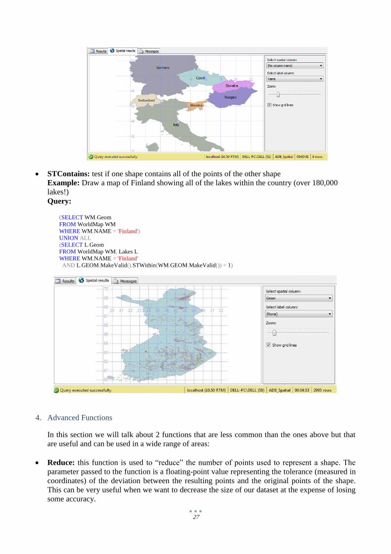
STContains: test if one shape contains all of the points of the other shape

Example: Draw a map of Finland showing all of the lakes within the country (over 180,000

lakes!)

Query:

(SELECT WM.Geom

FROM WorldMap WM

WHERE WM.NAME = 'Finland')

UNION ALL

(SELECT L.Geom

FROM WorldMap WM, Lakes L

WHERE WM.NAME = 'Finland'

AND L.GEOM.MakeValid().STWithin(WM.GEOM.MakeValid()) = 1)

4. Advanced Functions

In this section we will talk about 2 functions that are less common than the ones above but that

are useful and can be used in a wide range of areas:

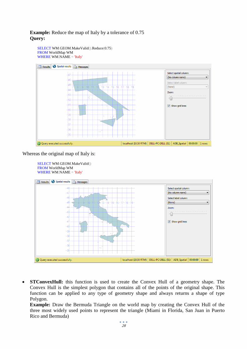
Reduce: this function is used to “reduce” the number of points used to represent a shape. The

parameter passed to the function is a floating-point value representing the tolerance (measured in

coordinates) of the deviation between the resulting points and the original points of the shape.

This can be very useful when we want to decrease the size of our dataset at the expense of losing

some accuracy.

28

Example: Reduce the map of Italy by a tolerance of 0.75

Query:

SELECT WM.GEOM.MakeValid().Reduce(0.75)

FROM WorldMap WM

WHERE WM.NAME = 'Italy'

Whereas the original map of Italy is:

SELECT WM.GEOM.MakeValid()

FROM WorldMap WM

WHERE WM.NAME = 'Italy'

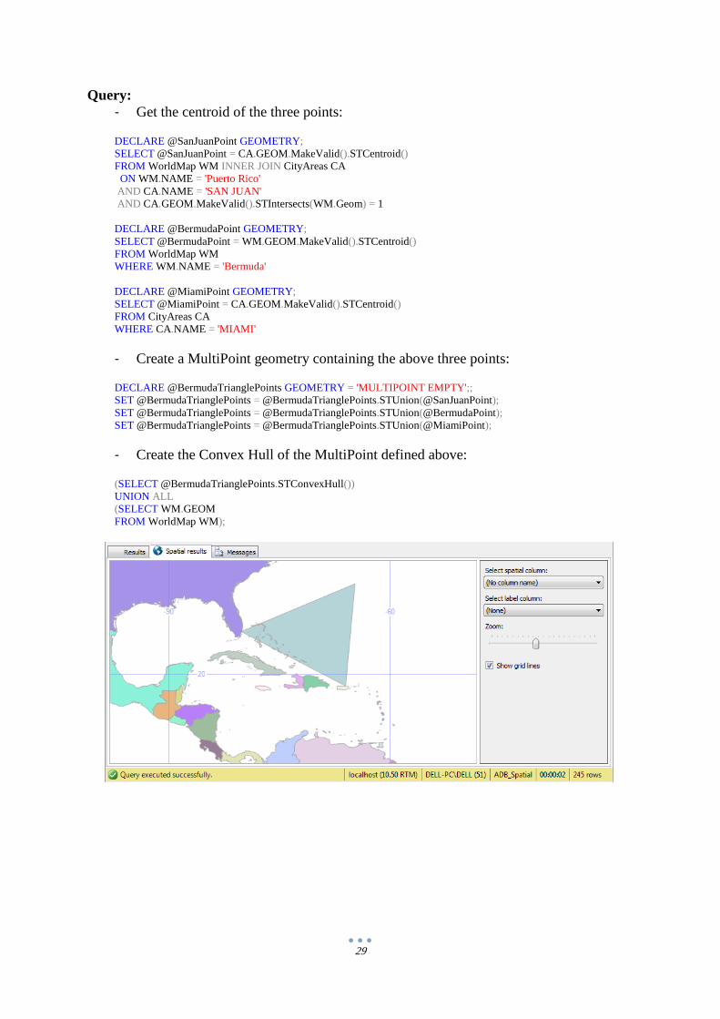
STConvexHull: this function is used to create the Convex Hull of a geometry shape. The

Convex Hull is the simplest polygon that contains all of the points of the original shape. This

function can be applied to any type of geometry shape and always returns a shape of type

Polygon.

Example: Draw the Bermuda Triangle on the world map by creating the Convex Hull of the

three most widely used points to represent the triangle (Miami in Florida, San Juan in Puerto

Rico and Bermuda)

29

Query:

- Get the centroid of the three points:

DECLARE @SanJuanPoint GEOMETRY;

SELECT @SanJuanPoint = CA.GEOM.MakeValid().STCentroid()

FROM WorldMap WM INNER JOIN CityAreas CA

ON WM.NAME = 'Puerto Rico'

AND CA.NAME = 'SAN JUAN'

AND CA.GEOM.MakeValid().STIntersects(WM.Geom) = 1

DECLARE @BermudaPoint GEOMETRY;

SELECT @BermudaPoint = WM.GEOM.MakeValid().STCentroid()

FROM WorldMap WM

WHERE WM.NAME = 'Bermuda'

DECLARE @MiamiPoint GEOMETRY;

SELECT @MiamiPoint = CA.GEOM.MakeValid().STCentroid()

FROM CityAreas CA

WHERE CA.NAME = 'MIAMI'

- Create a MultiPoint geometry containing the above three points:

DECLARE @BermudaTrianglePoints GEOMETRY = 'MULTIPOINT EMPTY';;

SET @BermudaTrianglePoints = @BermudaTrianglePoints.STUnion(@SanJuanPoint);

SET @BermudaTrianglePoints = @BermudaTrianglePoints.STUnion(@BermudaPoint);

SET @BermudaTrianglePoints = @BermudaTrianglePoints.STUnion(@MiamiPoint);

- Create the Convex Hull of the MultiPoint defined above:

(SELECT @BermudaTrianglePoints.STConvexHull())

UNION ALL

(SELECT WM.GEOM

FROM WorldMap WM);

30

Observations

In this section, we will talk about some of the observations / difficulties we faced while dealing with

SQL Server 2008 spatial features:

Visualization Limit

Although SQL Server Management Studio 2008 has native support for visualization of spatial data, it

does have a lot of limitations in that area. Namely, we faced the following difficulties:

- We can only visualize one spatial column at a time: this made some simple queries a bit more

complex to handle since we cannot display more than one spatial column

- We can only display 5000 spatial objects: we faced this problem when trying to display all

the railroads in Germany, which is a fairly simple example compared to most real-world

applications

This demonstrated the limitations of the visualization capabilities of SQL Server MS 2008 and

hence, we recommend the use of another visualization tool when developing real-world spatial

applications

Filter vs. STIntersects

Earlier in the report, we demonstrated the difference between the functions Filter and STIntersects

and the results showed that Filter performs the intersection much faster. However, since Filter only

does an approximate intersection test, this might produce erroneous results in some queries such as

in the example explained below.

Assume we want to draw a map of all the railroads passing through the city of Munich. Let’s first

use the STIntersects function as follows:

(SELECT CA.Geom

FROM CityAreas CA

WHERE CA.NAME = 'MUNICH')

UNION ALL

(SELECT R.Geom

FROM CityAreas CA, RAILROADS R

WHERE CA.NAME = 'MUNICH'

AND CA.GEOM.STIntersects(R.GEOM) = 1)

31

Now, notice how executing the same query with Filter gives us different results:

(SELECT CA.Geom

FROM CityAreas CA

WHERE CA.NAME = 'MUNICH')

UNION ALL

(SELECT R.Geom

FROM CityAreas CA, RAILROADS R

WHERE CA.NAME = 'MUNICH'

AND CA.GEOM.Filter(R.GEOM) = 1)

This difference in results is due to the fact that Filter only does approximate intersection test. Hence,

one should be careful when using the Filter function because it might give different – usually

erroneous – results.

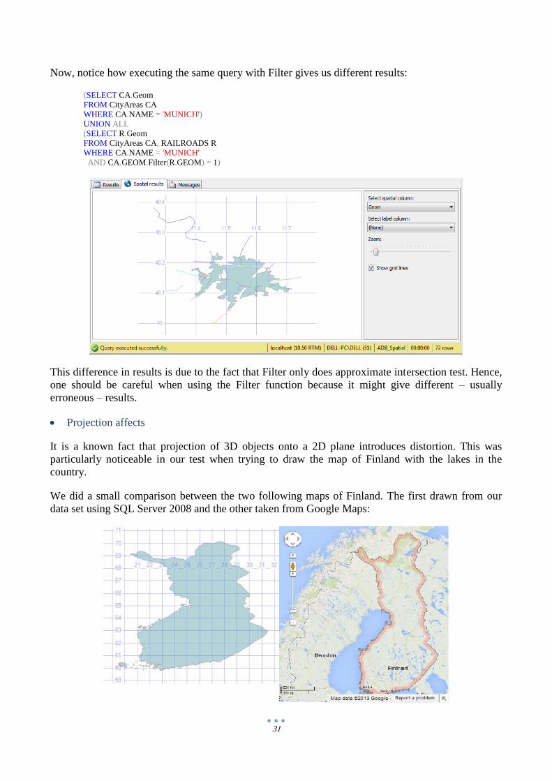
Projection affects

It is a known fact that projection of 3D objects onto a 2D plane introduces distortion. This was

particularly noticeable in our test when trying to draw the map of Finland with the lakes in the

country.

We did a small comparison between the two following maps of Finland. The first drawn from our

data set using SQL Server 2008 and the other taken from Google Maps:

32

What seems to be an extreme difference in the shape of the country is merely a difference in the

projection type used. This distortion becomes particularly clear near the poles and that is why it is

specifically obvious in the map of Finland.

Conclusion

During this project, we have identified the main definitions in the topic of spatial data and explored

what SQL Server 2008 has to offer in support of this ever-growing field.

We first explained how spatial data is represented and handled in SQL Server 2008 and then moved

to a case study wherein we implemented several queries that demonstrate the spatial capabilities of

SQL Server 2008 against a sample data set consisting of 2D projected geometry shapes.

While most of the basic functions would work similarly on the Geography data type, the limited

scope of the project meant that the Geography data type could not be explored in more depth.

Regarding the data used in the project, despite its limitations, such as the need to use the

MakeValid() function explained in the report, it was comprehensive and varied enough to fit the

purpose of this project.

In general, we can say that we have explored spatial data support in SQL Server 2008 to a degree

where we can implement a real-world application with ease.

33

Bibliography

Aitchison, A. (2009). Beginning Spatial with SQL Server 2008. Apress.

Yeung, A., & Hall, B. (2007). Spatial Database Systems, Design, Implementation and Project

Management. Dordrecht, The Netherlands: Springer.

Belussi, A., Catania, B., Clementini, E., & Ferrari, E. (2007). Spatial Data on the Web. Berlin:

Springer.

Boston Geographic Information Systems. (2008, May/June). Boston Geographic Information

Systems. Retrieved 11 9, 2013, from Boston Geographic Information Systems:

http://www.bostongis.com/PrinterFriendly.aspx?content_name=sqlserver2008_postgis_mysql_comp

are

ESRI. (n.d.). What is ArcGIS? Retrieved 11 30, 2013, from ArcGIS Resource Center:

http://resources.arcgis.com/en/help/getting-started/articles/026n00000014000000.htm

Microsoft. (n.d.). Reporting Services (SSRS). Retrieved 11 30, 2013, from Microsoft Developer

Network: http://msdn.microsoft.com/en-gb/library/ms159106(v=sql.105).aspx

Open Jump. (2011). Open Jump GIS. Retrieved 11 30, 2013, from http://www.openjump.org

Shekar, S., & Chawla, S. (2003). Spatial Databases: A Tour. Upper saddle River, NJ: Pearson

Education Inc.