Spatial and temporal variation of total electron content ... · mvs. mand R2 M vs. Mfor the daily ... Spatial and temporal variation of total electron content 1111 ... wave structure

Ann. Geophys., 34, 1109–1117, 2016www.ann-geophys.net/34/1109/2016/doi:10.5194/angeo-34-1109-2016© Author(s) 2016. CC Attribution 3.0 License.

Spatial and temporal variation of total electron content as revealedby principal component analysisElsayed R. Talaat1,a and Xun Zhu1

1The Johns Hopkins University Applied Physics Laboratory, 11100 Johns Hopkins Road, Laurel, MD 20723, USAanow at: Heliophysics Division, NASA Headquarters, Washington, D.C. 20546, USA

Correspondence to: Xun Zhu ([email protected])

Received: 14 July 2016 – Revised: 30 September 2016 – Accepted: 6 November 2016 – Published: 29 November 2016

Abstract. Eleven years of global total electron content (TEC)data derived from the assimilated thermosphere–ionosphereelectrodynamics general circulation model are analyzed us-ing empirical orthogonal function (EOF) decomposition andthe corresponding principal component analysis (PCA) tech-nique. For the daily averaged TEC field, the first EOF ex-plains more than 89 % and the first four EOFs explain morethan 98 % of the total variance of the TEC field, indicating aneffective data compression and clear separation of differentphysical processes. The effectiveness of the PCA techniquefor TEC is nearly insensitive to the horizontal resolution andthe length of the data records. When the PCA is applied toglobal TEC including local-time variations, the rich spatialand temporal variations of field can be represented by thefirst three EOFs that explain 88 % of the total variance. Thespectral analysis of the time series of the EOF coefficients re-veals how different mechanisms such as solar flux variation,change in the orbital declination, nonlinear mode couplingand geomagnetic activity are separated and expressed in dif-ferent EOFs. This work demonstrates the usefulness of usingthe PCA technique to assimilate and monitor the global TECfield.

Keywords. Ionosphere (ionospheric disturbances)

1 Introduction

The ionosphere is highly variable and has a complex systemof drivers including variable solar radiation plus geomagneticactivity from the upper atmosphere and momentum and en-ergy fluxes associated with neutral wind dynamics from thelower atmosphere. While magnetospheric forcing dominatesthe variability at high latitudes in the ionosphere, photochem-

istry and neutral dynamics play dominant roles in the iono-spheric structure and variability at mid- and low latitudes.One critical quantity describing the ionosphere and its vari-ability is the total electron content (TEC). A variety of in situand remote-sensing techniques has been employed to studythe Earth’s ionosphere in terms of the electron density. Themethod and platform used for measurement determine reso-lution in time and space, with the measurement often beingdistributed unevenly. Unless assimilated general circulationmodels are used, no one method effectively allows for thesampling of large areas of the ionosphere with high and uni-form resolution in both time and space. Since ionosphericelectronic densities respond to a complex set of highly vari-able driving mechanisms, the global characterization of theresponse to solar variability posts a significant challenge.

The X-ray and ultraviolet solar irradiance which createsthe ionosphere varies on all timescales: with an 11-year solarcycle associated with the 22-year magnetic cycle of the so-lar dynamo, with a quasi-27-day period due to active regionsrotating with the sun, and on the order of minutes to hoursas eruptions occur on the disk of the sun (Lean, 1987; To-biska, 1993). The ionosphere varies on all these timescalesin response to the solar inputs, while the geographic rela-tionship of the Earth’s orbit, rotation and seasonal tilt createsthe solar zenith angle dependence that yields the observeddiurnal, seasonal and annual variations in ionospheric den-sity. This is further complicated by the tilt of the magneticfield of Earth, the magnetospheric inputs that drive the iono-sphere at high latitudes, and the neutral dynamics generatedby solar and magnetospheric forcing, indicating significantlongitudinal and hemispherical asymmetries in space. Thus,the multi-scale variability and complexity in both time and

Published by Copernicus Publications on behalf of the European Geosciences Union.

1110 E. R. Talaat and X. Zhu: Spatial and temporal variation of total electron content

space induced by different kinds of physical processes arethe main characteristics of the ionosphere.

In this paper, we perform a set of multi-year assimilatedruns of the thermosphere–ionosphere electrodynamics gen-eral circulation model (TIEGCM) (Roble et al., 1988; Rich-mond et al., 1992) driven by a lower boundary condition oftidal forcing derived from the Sounding of the Atmosphereusing Broadband Emission Radiometry (SABER) instrument(Talaat and Lieberman, 1999; Talaat et al., 2001). To effec-tively decompose and understand the complicated temporaland spatial variations of the ionosphere, we apply the empir-ical orthogonal function (EOF) and the associated principalcomponent analysis (PCA) to the TEC fields derived from theTIEGCM runs. Section 2 describes the EOF and PCA nota-tions and their application to different TEC fields. Section 3shows how the EOF and PCA are able to reveal major phys-ical processes associated with different EOFs derived fromdata fields. Section 4 provides a final summary and conclu-sions.

2 EOF and PCA of the assimilated TEC

2.1 A brief review and notations of the EOF and PCA

The empirical orthogonal function (EOF) and the corre-sponding principal component analysis (PCA) are the stan-dard statistical techniques for analyzing atmospheric datasince being introduced by E. N. Lorenz in 1956 (Wilks,2006). The PCA technique decomposes a given spatial–temporal field such as TEC into a set of base functionscalled EOFs that is internally determined from the datasets. Let un = un,ij = u(tn;xi,yj ) denote the time series ofthe measured or the assimilated TEC field at N time stepsoverK = I×J spatial grids (n= 1,2, . . .,N ; i = 1,2, . . ., I ;j = 1,2, . . .,J ), where tn, xi and yj denote time, longi-tude and latitude, respectively. Then, the PCA expressesthe spatial–temporal field un by its time-averaged field u(=

N−16Nn=1un) and a set of EOFs (vm, m= 1,2, . . .,K) thatdo not vary with time (Preisendorfer, 1988, Wilks, 2006):

un = u+u′n = u+

K∑m=1

Em,nvm,n= 1,2, . . .,N, (1)

where the principal component (PC) Em,n is the time seriesof the decomposition coefficient that characterizes the tem-poral variation of the original field un being projected ontothe mth EOF vm. Furthermore, different PCs are orthogonalto each other in time (Preisendorfer, 1988).

Equation (1) is a reconstruction formula and can be con-sidered as a linear transform that projects the original pertur-bation field un− u onto a set of base functions {vm}. SinceEOFs are derived from the data rather than prescribed basefunctions such as spherical harmonic functions that are oftenused for analyzing global data, the most information on the

original field that represents the physics and its variations canbe expressed by a highly truncated Eq. (1) with M �K ,

un ≈ u+

M∑m=1

En,mvm,n= 1,2, . . .,N. (2)

The effectiveness of the PCA can be quantitatively measuredby the ratio of the percentage of the total variance in un− u

explained by individual EOFs:

r2m =

Var(Em,nvm)Var(un− u)

× 100%. (3)

The value of r2m is proportional to the magnitude of the mth

eigenvalue (λm) of the covariance matrix of un− u that de-creases with m (Wilks, 2006). Since different EOFs are or-thogonal to each other in space, the explained variance by thetruncated PCA expression Eq. (2) for differentM is given by

R2M =

M∑m=1

r2m. (4)

2.2 EOF and PCA applied to daily averaged TEC

We ran the TIEGCM with realistic solar inputs and tidal forc-ing over the 11-year time period from 1990 to 2010. The hor-izontal resolution of the TEC field is 5◦× 2.5◦, which corre-sponds to K = 72× 71= 5112 spatial grids. In Fig. 1, weshow the plots of r2

m vs. m and R2M vs. M for the daily av-

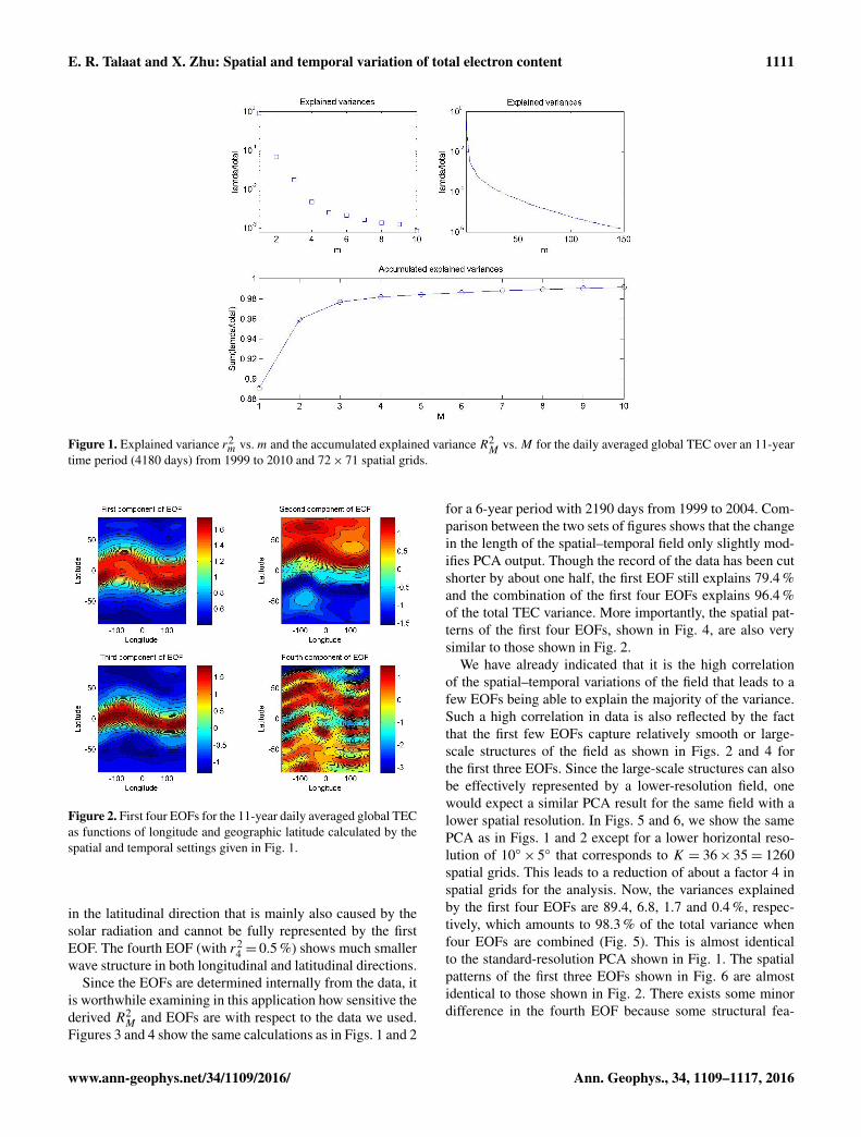
eraged global TEC over an 11-year period with 4180 days(1999–2010). The most striking feature is that the first EOFhas already explained 89 % of the total variance. The combi-nation of the first four EOFs explains more than 98 % of thetotal variance. The fact that R2

M > 98 % forM = 4 shows theeffectiveness of the PCA on data compression or informationrepresentation in this particular example. Here, the effective-ness of the data compression of PCA is mainly due to thefollowing two reasons: (i) the base functions have been in-ternally derived from data rather than externally prescribedand (ii) there exist substantial correlations among data ondifferent spatial and temporal grids. In Fig. 2, we show thefirst four EOFs for the 11-year daily averaged global TEC asfunctions of longitude and geographic latitude. Note that thefirst component explains the majority (with r2

1 = 89.1 %) ofthe spatial variance of TEC. It represents the combined ef-fects of solar radiation that makes the TEC decrease with lat-itude and geomagnetic field that produces a zonal wave num-ber 1 structure due the offsetting of the geomagnetic poles.Note that the electrons produced by the photoionization aresymmetric with respect to geographic poles, whereas thoseproduced by the energetic particle precipitation are symmet-ric with respect to the geomagnetic poles. The second EOF(with r2

2 = 6.9 %) captures the interhemispheric asymmetryof the TEC, mainly caused by the seasonal variation of theinclination angle of the Earth’s orbit. The third EOF (withr2

3 = 1.7 %) represents the narrower or finer structure of TEC

Ann. Geophys., 34, 1109–1117, 2016 www.ann-geophys.net/34/1109/2016/

E. R. Talaat and X. Zhu: Spatial and temporal variation of total electron content 1111

Figure 1. Explained variance r2m vs.m and the accumulated explained variance R2

Mvs.M for the daily averaged global TEC over an 11-year

time period (4180 days) from 1999 to 2010 and 72× 71 spatial grids.

Figure 2. First four EOFs for the 11-year daily averaged global TECas functions of longitude and geographic latitude calculated by thespatial and temporal settings given in Fig. 1.

in the latitudinal direction that is mainly also caused by thesolar radiation and cannot be fully represented by the firstEOF. The fourth EOF (with r2

4 = 0.5 %) shows much smallerwave structure in both longitudinal and latitudinal directions.

Since the EOFs are determined internally from the data, itis worthwhile examining in this application how sensitive thederived R2

M and EOFs are with respect to the data we used.Figures 3 and 4 show the same calculations as in Figs. 1 and 2

for a 6-year period with 2190 days from 1999 to 2004. Com-parison between the two sets of figures shows that the changein the length of the spatial–temporal field only slightly mod-ifies PCA output. Though the record of the data has been cutshorter by about one half, the first EOF still explains 79.4 %and the combination of the first four EOFs explains 96.4 %of the total TEC variance. More importantly, the spatial pat-terns of the first four EOFs, shown in Fig. 4, are also verysimilar to those shown in Fig. 2.

We have already indicated that it is the high correlationof the spatial–temporal variations of the field that leads to afew EOFs being able to explain the majority of the variance.Such a high correlation in data is also reflected by the factthat the first few EOFs capture relatively smooth or large-scale structures of the field as shown in Figs. 2 and 4 forthe first three EOFs. Since the large-scale structures can alsobe effectively represented by a lower-resolution field, onewould expect a similar PCA result for the same field with alower spatial resolution. In Figs. 5 and 6, we show the samePCA as in Figs. 1 and 2 except for a lower horizontal reso-lution of 10◦× 5◦ that corresponds to K = 36× 35= 1260spatial grids. This leads to a reduction of about a factor 4 inspatial grids for the analysis. Now, the variances explainedby the first four EOFs are 89.4, 6.8, 1.7 and 0.4 %, respec-tively, which amounts to 98.3 % of the total variance whenfour EOFs are combined (Fig. 5). This is almost identicalto the standard-resolution PCA shown in Fig. 1. The spatialpatterns of the first three EOFs shown in Fig. 6 are almostidentical to those shown in Fig. 2. There exists some minordifference in the fourth EOF because some structural fea-

www.ann-geophys.net/34/1109/2016/ Ann. Geophys., 34, 1109–1117, 2016


Figure 3. Same as Fig. 1 except for a 6-year time period (2190 days) from 1999 to 2004.

Figure 4. Same as Fig. 2 except for a 6-year time period (2190 days)from 1999 to 2004.

tures cannot be fully resolved by a lower-resolution analysis(r2

4 = 0.4 % in Fig. 1 vs. r24 = 0.5 % in Fig. 5).

2.3 EOF and PCA applied to hourly TEC

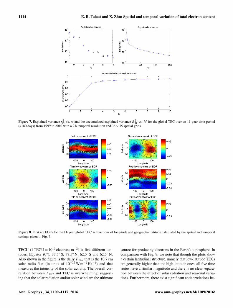
Next, we examine the TEC field that includes the local-timevariations. The PCA is applied to the u(tn;xi,yj ) field withthe lower-resolution spatial grid of Figs. 5 and 6 but witha temporal resolution of 2 h. The total number of time stepsN = 50 160, which corresponds to 11.4 years of time intervalstarting from 1999. Figures 7 and 8 show plots of (r2

m,R2M)

and the first six EOFs. We first note that (Fig. 7) the contribu-tion by the first EOF (48.8 %) is significantly lower than oneshown in the daily averaged TEC analysis (Figs. 1, 3 and 5),indicating a weaker correlation or a richer structure in spatialand temporal variability of the TEC field. This is expectedsince unlike the daily averaged field, the local-time varia-tion introduces additional and stronger longitudinal varia-tions due to the local-time response of TEC that is directlyrelated to the solar radiation forcing. The sum of the firstsix EOFs makes up approximately 93.6 % of the total vari-ance. Another significant feature shown in Fig. 7 is that thesecond and third EOFs contribute almost equally (20.4 and18.6 %) to the total variance. The spatial pattern of the firstEOF in Fig. 8 is almost identical to that shown in Fig. 2,mainly representing the effects of daily averaged solar forc-ing and the dominant wave number 1 feature due to the off-setting geomagnetic field. The next two EOFs shown in Fig. 8represent longitudinal variation of wave number 1 with ap-proximately equal magnitudes and π/2 phase shift. Thesetwo natural modes represent the major contributions from thefirst two components of the sinusoidal decomposition in lon-gitude sin(πxi/180) and cos(πxi/180) caused by the local-time solar forcing, which are not present in the daily averagedTEC field. The fourth and fifth EOFs in Fig. 8 once again ap-proximately duplicate the second and third EOFs in Fig. 2.In other words, because different EOFs are orthogonal, theincrease in resolution in TEC data only adds new modes toPCA but has little effect on the existing modes in the lower-resolution PCA. The sixth EOF mainly represents the lon-gitudinal variation of wave number 2. Note that the paired(r2

6 , r27 ) and (r2

8 , r29 ) shown in Fig. 7 are similar to (r2

2 , r23 )

and have nearly equal magnitudes of the explained variance.



Figure 5. Same as Fig. 1 except for a spatial resolution of 36× 35 grids.

Figure 6. Same as Fig. 2 except for a spatial resolution of 36× 35grids.

One expects that the paired EOFs (v6,v7) and (v8,v9) rep-resent the high harmonics of the longitudinal variance asso-ciated with the local-time variation of the solar forcing. Wehave also performed sensitivity analyses for the case simi-lar to Figs. 3 and 4 by applying PCA to shorter data recordsof 4 years that correspond to either solar maximum (1999–2003) or solar minimum (2006–2009). In terms of their spa-tial structure, the derived EOFs are almost identical to thoseshown in Fig. 8.

3 Physical processes as objectively revealed by EOFsand TEC

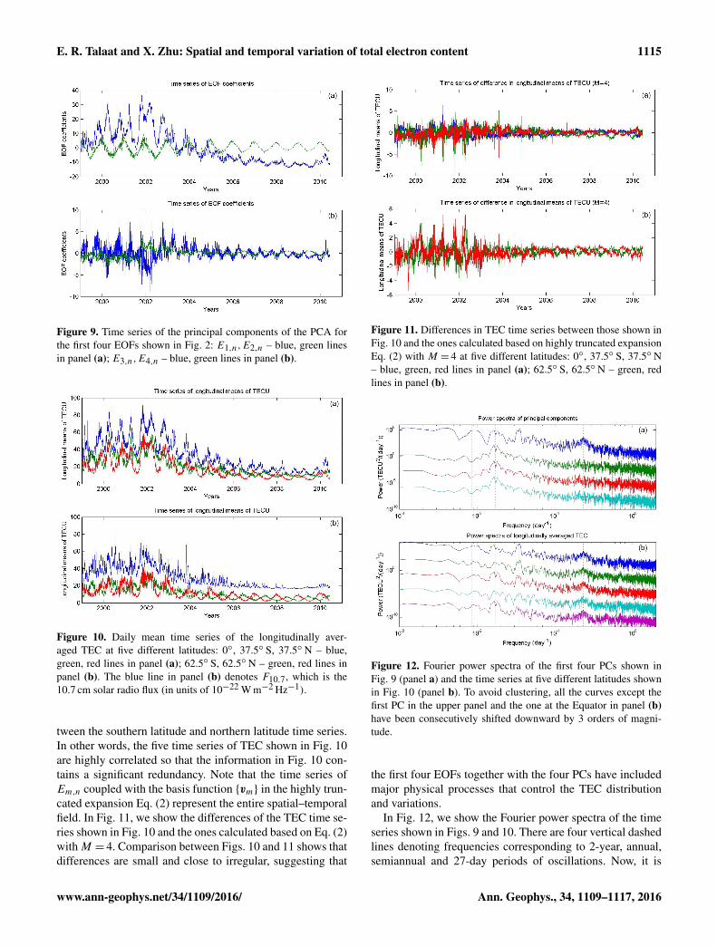
One major advantage of the PCA technique is the data com-pression, so the physical field is effectively projected onto afew modes that include the majority of the variance of theoriginal field. We have already shown that the four EOFs inFig. 2 and the six EOFs in Fig. 8 contain 98.2 and 93.6 %of the total variance, respectively. Based on their spatial pat-terns, we have also indicated in the above analysis that thereexist clear physical mechanisms that drive the different EOFssolely derived from the data. To illustrate the roles played bydifferent physical mechanisms in extracting EOFs, we showin Fig. 9 the time series of the decomposition coefficientsEm,n, i.e., PCs, of the PCA for the first four EOFs, shown inFig. 2. The specific physical mechanisms are best describedin by E1,n and E2,n. Since v1 and v2 in Fig. 2 mainly repre-sent the effects of the solar radiation and the seasonal varia-tion of the inclination angle of the Earth’s orbit, the two timeseries plotted in the upper panel of Fig. 9 show the responsesof the 11-year solar cycle and annual oscillation. Note thatthe variance contributed from v3 and v4 is far less than thosefrom v1 and v2 (Fig. 1). This is also reflected by the factthat the magnitudes of E3,n and E4,n are much smaller thanthose of E1,n and E2,n. Furthermore, since neither effect ofthe solar radiation nor the seasonal variation is orthogonal inspace, the remaining EOFs, including v3 and v3 together withtheir coefficients Em,n, will include both effects, as indicatedabove and also shown in the lower panel of Fig. 9.

To further demonstrate the benefit of the PCA techniquein the current application, we show in Fig. 10 the timeseries of the longitudinally averaged TEC in the unit of



Figure 7. Explained variance r2m vs. m and the accumulated explained variance R2

Mvs. M for the global TEC over an 11-year time period

(4180 days) from 1999 to 2010 with a 2 h temporal resolution and 36× 35 spatial grids.

Figure 8. First six EOFs for the 11-year global TEC as functions of longitude and geographic latitude calculated by the spatial and temporalsettings given in Fig. 7.

TECU (1 TECU= 1016 electrons m−2) at five different lati-tudes: Equator (0◦), 37.5◦ S, 37.5◦ N, 62.5◦ S and 62.5◦ N.Also shown in the figure is the daily F10.7 that is the 10.7 cmsolar radio flux (in units of 10−22 W m−2 Hz−1) and thatmeasures the intensity of the solar activity. The overall cor-relation between F10.7 and TEC is overwhelming, suggest-ing that the solar radiation and/or solar wind are the ultimate

source for producing electrons in the Earth’s ionosphere. Incomparison with Fig. 9, we note that though the plots showa certain latitudinal structure, namely that low-latitude TECsare generally higher than the high-latitude ones, all five timeseries have a similar magnitude and there is no clear separa-tion between the effect of solar radiation and seasonal varia-tions. Furthermore, there exist significant anticorrelations be-



Figure 9. Time series of the principal components of the PCA forthe first four EOFs shown in Fig. 2: E1,n,E2,n – blue, green linesin panel (a); E3,n,E4,n – blue, green lines in panel (b).

Figure 10. Daily mean time series of the longitudinally aver-aged TEC at five different latitudes: 0◦, 37.5◦ S, 37.5◦ N – blue,green, red lines in panel (a); 62.5◦ S, 62.5◦ N – green, red lines inpanel (b). The blue line in panel (b) denotes F10.7, which is the10.7 cm solar radio flux (in units of 10−22 W m−2 Hz−1).

tween the southern latitude and northern latitude time series.In other words, the five time series of TEC shown in Fig. 10are highly correlated so that the information in Fig. 10 con-tains a significant redundancy. Note that the time series ofEm,n coupled with the basis function {vm} in the highly trun-cated expansion Eq. (2) represent the entire spatial–temporalfield. In Fig. 11, we show the differences of the TEC time se-ries shown in Fig. 10 and the ones calculated based on Eq. (2)withM = 4. Comparison between Figs. 10 and 11 shows thatdifferences are small and close to irregular, suggesting that

Figure 11. Differences in TEC time series between those shown inFig. 10 and the ones calculated based on highly truncated expansionEq. (2) with M = 4 at five different latitudes: 0◦, 37.5◦ S, 37.5◦ N– blue, green, red lines in panel (a); 62.5◦ S, 62.5◦ N – green, redlines in panel (b).

Figure 12. Fourier power spectra of the first four PCs shown inFig. 9 (panel a) and the time series at five different latitudes shownin Fig. 10 (panel b). To avoid clustering, all the curves except thefirst PC in the upper panel and the one at the Equator in panel (b)have been consecutively shifted downward by 3 orders of magni-tude.

the first four EOFs together with the four PCs have includedmajor physical processes that control the TEC distributionand variations.

In Fig. 12, we show the Fourier power spectra of the timeseries shown in Figs. 9 and 10. There are four vertical dashedlines denoting frequencies corresponding to 2-year, annual,semiannual and 27-day periods of oscillations. Now, it is



Figure 13. Time series of the principal components of the PCA forthe first EOFs shown in Fig. 8: Eamp,E1,n,E4,n – blue, green, redlines.

Figure 14. Scatterplots between the daily averaged F10.7 and thedaily averaged time series (Eamp,E1,n,E4,n) shown in Fig. 13:(Eamp,E1,n,E4,n) – (blue, green, red) dots.

more clearly and quantitatively shown in the figure that themajor spectral features among different EOFs are different,whereas those among the longitudinally averaged TEC at dif-ferent latitudes are nearly the same. The first EOF spectrumpeaks at all four frequencies, whereas the second EOF onlyshows one striking peak in the annual period that is domi-nant over the entire spectral domain. For the third and fourthEOFs, only two peaks at semiannual and 27-day periods arenoticeable. Since different spectral characters often corre-spond to different driving mechanisms, Fig. 12 suggests thatthe PCA technique is able to differentiate directly betweenphysical mechanisms and the data.

Figure 15. Two-hour resolution time series of the longitudinallyaveraged TEC at five different latitudes: 0◦, 40◦ S, 40◦ N – blue,green, red lines in panel (a); 60◦ S, 60◦ N – green, red lines inpanel (b).

Figure 13 shows the time series of PCA for the case ofFig. 8, which includes local-time variation Eamp, E1,n andE4,n, where Eamp is the amplitude of the time series for thepaired EOFs (v2,v3):

Eamp =

√(E2,n

)2+(E3,n

)2,

Ephase = tan−1 (E3,n/E2,n). (5)

Note that the paired EOFs (v2,v3) shown in Fig. 8 denotethe fixed spatial patterns of the local-time variations with aπ/2 phase shift. As a result, the corresponding paired coef-ficients (E2,n,E3,n) are expected to have similar magnitudesand change rapidly with the local time in order to representa moving wave structure. The amplitude defined in Eq. (5)combines the effects of both components and also eliminatesthe local-time variation. We also note from Fig. 13 that E1,nand Eamp are highly correlated with a dominant period ofabout half a year though E1,n is not correlated with eitherE2,n or E3,n. This is because the first three EOFs all repre-sent the effect of solar radiation. On the other hand, the fourthEOF shows a clear signature of annual cycle that correspondsto the effect of the inclination angle of the Earth’s orbit. Sucha difference in the effects of solar radiation on the differ-ent EOF components can also be seen from Fig. 14, whichshows the scatterplots between the daily averaged F10.7 andthe daily averaged time series (Eamp,E1,n,E4,n) shown inFig. 13. The figure shows that F10.7 is well correlated withboth E1,n and Eamp, whereas E4,n appears to be insensi-tive to F10.7 variations. Figure 15 shows the time series ofthe longitudinally averaged TEC at five different latitudes:Equator (0◦), 40◦ S, 40◦ N, 60◦ S and 60◦ N. Comparing thisto Fig. 10, which also includes the local-time average, wenote the significant increase in daily variability of TEC, sug-



Figure 16. Fourier power spectra of the first four PCs shown inFig. 13 (panel a) and the time series at five different latitudes shownin Fig. 14 (panel b). To avoid clustering, the green and red curvesin (a) have been moved down by 3 and 6 orders of magnitude, re-spectively. All the curves except the one at the Equator in (b) havebeen consecutively shifted downward by 3 orders of magnitude. Thecyan curve in panel a denotes the spectrum of the phase 104Ephasedefined in Eq. (5).

gesting that the longitudinal and local-time averages are notinterchangeable for the TEC field.

In Fig. 16, we show the Fourier power spectra for the timeseries shown in Figs. 13 and 15. The six vertical lines denotethe peak frequencies that correspond to the following peri-ods: annual, semiannual, 27-day, 1-day, 0.5-day and 0.25-day. Panel a in the figure shows that Eamp has significantspectral peaks in all the noted frequencies, whereas Ephasedoes not show spectral peaks at the 27-day and semiannualperiods. We also note that there are significant sub-harmonicpeaks in the Eamp spectrum for a frequency greater than2π /1-day. The spectral peaks at 3π /1-day and 5π /1-day re-sult from the sum of spectral peaks at 2π /1-day plus π /1-dayand 3π /1-day plus 2π /1-day, respectively. Again, the spectralfeatures of Eamp are similar to that for the third EOF shownin Fig. 13, whereas the spectrum for the fourth EOF is dom-inated by the annual cycle, also consistent with the resultsshown in Fig. 13.

4 Summary and conclusions

In this study, we apply the EOF and PCA to the global TECdata derived from TIEGCM forced under the realistic solarinputs from above the SABER-observed tidal waves from be-low. We demonstrate the effectiveness of the EOF decompo-sition of the ionospheric variations in both time and space.It is shown that for the daily averaged TEC field, the firstEOF explains more than 89 % and the first four EOFs ex-

plain more than 98 % of the total variance of the TEC field.When PCA is coupled with the spectral analysis of the timeseries of the EOF coefficients, it is also shown that the EOFanalysis is not only a data compression technique but also apowerful tool to objectively reveal the relative importance ofindividual physical mechanisms (such as solar flux variation,change in the orbital declination, nonlinear mode couplingand geomagnetic activity) that are responsible for the totalTEC variance.

5 Data availability

The TIEGCM output TEC fields that generated allthe figures in this paper are available from Xun Zhu([email protected]) upon request.

Acknowledgements. This research was supported by NASA Liv-ing With a Star Program under grants NNX09AJ61G andNNX13AF91G and the Heliophysics Supporting Research programunder grant NNX16AG68G to the Johns Hopkins University Ap-plied Physics Laboratory. Comments on the paper by two anony-mous reviewers are greatly appreciated.

The topical editor, K. Shiokawa, thanks two anonymous refereesfor help in evaluating this paper.

References

Lean, J.: Solar ultraviolet irradiance variations: A review, J. Geo-phys. Res., 92, 839–868, 1987.

Preisendorfer, R. W.: Principal Component Analysis in Meteorol-ogy and Oceanography, edited by: Mobley, C. D., Elsevier, Am-sterdam, the Netherlands, 425 pp., 1988.

Richmond, A. D., Ridley, E. C., and Roble, R. G.: A thermo-sphere/ionosphere general circulation model with coupled elec-trodynamics, Geophys. Res. Lett., 19, 601–604, 1992.

Roble, R. G., Ridley, E. C., and Richmond, A. D.: A coupled ther-mosphere/ionosphere general circulation model, Geophys. Res.Lett., 15, 1325–1328, 1988.

Talaat, E. R. and Lieberman, R. S.: Nonmigrating diurnal tidesin the mesosphere and lower thermosphere, J. Atmos. Sci., 56,4073–4087, 1999.

Talaat, E. R., Yee, J.-H., and Zhu, X.: Observations of the 6.5-daywave in the mesosphere and lower thermosphere, J. Geophys.Res., 106, 20715–20724, doi:10.1029/2001JD900227, 2001.

Tobiska, W. K.: Recent solar extreme ultraviolet irradiance obser-vations and modeling: A review, J. Geophys. Res., 98, 18879–18893, 1993.

Wilks, D. S.: Statistical Methods in the Atmospheric Sciences, Sec-ond Edition, Academic Press, New York, USA, 627 pp., 2006.


http://dx.doi.org/10.1029/2001JD900227

Documents

Spatial and temporal variation of total electron content ... · mvs. mand R2 M vs. Mfor the daily ... Spatial and temporal variation of total electron content 1111 ... wave structure