Embed Size (px)
Citation preview
RESEARCH ARTICLE
Spatial versus temporal variation in precipitationin a semiarid ecosystem
David J. Augustine
Received: 12 March 2009 / Accepted: 26 February 2010
� US Government 2010
Abstract Spatial and temporal variations in precip-
itation are central features of semiarid ecosystems,
influencing patterns of plant productivity and the
distribution of native fauna. Although temporal
variation in precipitation has been studied exten-
sively, far less is known about the spatial scale and
pattern of precipitation variability in semiarid
regions. I used long-term precipitation records to
examine spatial variation across the 63 km2 Central
Plains Experimental Range in northeastern Colorado,
and across the 117,000 km2 region of shortgrass
steppe in eastern Colorado. Relative to temporal
variation, spatial variation was low at scales\10 km,
increased linearly across scales of 40–120 km, and
was nearly equal in magnitude to temporal variation
across distances of 120–160 km. Although I hypoth-
esized that most spatial variation would be generated
by early-summer convective thunderstorms in June, I
found that the magnitude and spatial pattern of
variation was similar for precipitation received in
June compared to cumulative precipitation received
during the full growing season. The degree of spatial
autocorrelation in precipitation across all distances
that I evaluated was similar for drought, dry, above-
average and wet years. Across distances of 10–
120 km, spatial variation within a single growing
season was approximately two times greater than
spatial variation in long-term mean growing-season
precipitation, indicating spatial shifting in the loca-
tions of patches of high and low precipitation over
multiple years. Overall, these findings suggest spatial
variation at scales of 10–160 km may have been an
important factor influencing vegetation patterns and
migratory fauna of the shortgrass steppe, and have
implications for livestock producers and future
assessments of climate change.
Keywords Bison � Grassland birds �Rainfall � Shortgrass steppe � Spatiotemporal mosaic �Spatial heterogeneity � Migration
Introduction
Temporal variability in precipitation is a key factor
influencing the structure and function of semiarid
ecosystems (Knapp and Smith 2001; Austin et al. 2004;
Collins et al. 2008), but far less is known about the
scale and magnitude of spatial variation in precipita-
tion in semiarid regions. Variation in mean annual
precipitation (MAP) across gradients extending from
arid to mesic regions has been quantified and related to
ecosystem structure and function in many grasslands
and savannas worldwide (e.g. McNaughton 1985;
Williams et al. 1996; Lauenroth et al. 1999; Sankaran
et al. 2005). However, the scale and magnitude of
spatial variability within areas where long-term mean
D. J. Augustine (&)
USDA-ARS, Rangeland Resources Research Unit, 1701
Centre Avenue, Fort Collins, CO 80526, USA
e-mail: [email protected]
123
Landscape Ecol
DOI 10.1007/s10980-010-9469-y
precipitation is relatively constant has rarely been
quantified. Semiarid ecosystems are often character-
ized by vast expanses of flat to gently undulating
topography, where orographics have minimal influ-
ence on precipitation patterns. Within these land-
scapes, spatial variability in precipitation inputs can be
a consequence of local variation in the intensity and
path of convective thunderstorms. Because water
limitations influence nearly all aspects of semiarid
ecosystem function, an understanding of spatial vari-
ation in precipitation inputs in these regions can
provide insights to historic patterns of ecosystem
function and potentially guide future approaches to
ecosystem management and conservation.
In the grasslands of central North America, MAP
decreases from east to west, while interannual
variation in precipitation increases (Wiens 1972,
1974). The semiarid shortgrass steppe, located in the
westernmost and driest portion of the central North
American grasslands, is characterized by lower mean
annual precipitation (MAP * 300–550 mm) and
higher interannual variation in precipitation [coeffi-
cients of variation (CV) * 0.28] compared to mixed-
grass and tallgrass prairie (MAP * 500–730 cm,
CV * 0.23–0.26: Wiens 1972, 1974; Lauenroth and
Milchunas 1992; Lauenroth et al. 1999). Consider-
able research in the shortgrass steppe has demon-
strated the strong influence of temporal variation in
precipitation at scales from days to years on plants
and fauna (Wiens 1974; Sala and Lauenroth 1982;
Milchunas et al. 1994; Milchunas et al. 1998; Derner
et al. 2008). The Rocky Mountains that lie to the west
of the shortgrass steppe influence climate and weather
patterns due to the rain shadow they create (Pielke
and Doesken 2008), but topographic variation east of
the mountains, and its influence on movement of air
masses, is minimal. Topography is characterized by
gently undulating plains, with slopes typically 0–3%.
For example, at the Central Plains Experimental
Range in northeastern Colorado, typical catenas vary
by 6–21 m in elevation over 1.6 km (Milchunas et al.
1989) and elevation varies by only 25–90 m over
10 km. Within this flat landscape, more than 70% of
MAP falls during the growing season (April–Sep-
tember), and occurs during only 2–4% of the hours
within a year (Pielke and Doesken 2008). Factors
potentially contributing to spatial variation in precip-
itation include intense spring thunderstorms influ-
enced by sharp temperature contrasts in air masses,
and convective summer thunderstorms that bring
high-intensity rainfall over small areas for short
periods of time (Pielke and Doesken 2008). Despite
the central role of moisture limitation in semiarid
regions, I am unaware of studies that have examined
the relative magnitude of spatial versus temporal
variability in precipitation for these ecosystems.
Spatial variability in precipitation can potentially
influence and interact with many aspects of ecosystem
structure and function, but the influence may be
particularly strong for organisms with the capacity to
move across the landscape in response to spatial
variation. My interest in spatial precipitation patterns
was motivated by its implications for four aspects of
the ecology and management of semiarid ecosystems.
First, because bison were largely eliminated from
central North American grasslands prior to the onset
of ecological research, considerable speculation has
surrounded their distribution, abundance and role in
grassland dynamics (Bamforth 1987; Hart 2001; Lott
2002). Dry years were likely a primary determinant of
bison distribution and abundance, and spatial varia-
tion in precipitation at scales of\10 km to[100 km
may have influenced bison movement patterns, degree
of herd aggregation, and population dynamics (Lott
2002). Second, drought is a key limitation for
livestock management in semiarid regions today.
Long-distance movement of livestock in response to
spatially isolated rainfall has long been an important
strategy in semiarid rangelands outside of North
America (Coughenour 1991; McAllister et al. 2006).
Understanding the spatial scale of precipitation var-
iation during droughts can inform potential drought
mitigation strategies for livestock producers. Third,
bird communities in North American grasslands have
been strongly influenced by precipitation patterns
(Wiens 1974). Most bird species endemic to grass-
lands of central North America are migratory, hence
can respond to large-scale spatial variation in precip-
itation, and are also undergoing population declines
(Brennan and Kuvleskey 2005). The scale and mag-
nitude of spatial variation in precipitation may be an
important factor interacting with land use changes in
grasslands (Samson et al. 2004), and could inform
approaches for monitoring and mitigating declines in
grassland bird species. Fourth, quantification of
spatial patterns from long-term datasets can provide
an important baseline for assessing the reliability of
local precipitation predictions in unmeasured
Landscape Ecol
123
locations, and assessing future climate change.
Research sites even in areas of flat topography that
lack an on-site weather stations or rely on a single
station often do not know how precipitation varies
from station to research site, and precipitation can be a
particularly difficult variable to predict with a sparse
network of gauges (Hubbard 1994). Under future
climate change, increases in inter- and intra-annual
variability of precipitation are predicted (Meehl et al.
2007) but predictions are presented and discussed at
the scale of regions within continents, and cannot
address changes in spatial patterns across distances
\1,000 km (Christensen and Hewiston 2007). Under-
standing both spatial and temporal patterns of vari-
ability in precipitation over the past half-century is
essential to assessing future changes.
The objective of this study was to quantify the
magnitude and scale of spatial variation in growing-
season precipitation in the shortgrass steppe. The
analysis focused on precipitation records collected at
two spatial scales. First, I analyzed records from
stations distributed across the USDA-Agricultural
Research Service Central Plains Experimental Range
in northeastern Colorado to examine spatial variation
across distances of 1–8 km. Second, I analyzed
records from stations distributed across eastern Col-
orado, which covers approximately 117,000 km2 in
the northern half of the shortgrass steppe ecosystem
(Lauenroth and Milchunas 1992), to examine patterns
across distances of 10–200 km. Specific objectives
were to (1) test whether spatial variability in precip-
itation at local (1–8 km) and regional (10–200 km)
scales is inversely related to the amount of growing-
season precipitation, (2) compare the magnitude of
spatial variation in precipitation across scales of
1–200 km to inter-annual variability, and (3) quantify
the degree of patchiness in precipitation across spatial
scales in the shortgrass steppe, and whether such
patchiness differs between dry versus wet years.
Methods
Central plains experimental range
The Central Plains Experimental Range (CPER)
encompasses approximately 62.8 km2 of shortgrass
steppe located northeast of Nunn, Colorado (40�490Nlatitude, 107�470W longitude). CPER was established
in response to the abandonment of ranches and farms
during the 1930s, and has supported rangeland
research since 1939. Beginning in 1939, manual rain
gauges were established at 27 different locations on
the property, and have been monitored during May–
September each year. Gauges were always checked
within 60 h of a precipitation event, which limited
losses to evaporation to less than 0.025 mm, but
typically were checked 24 h after precipitation. Four
additional gauge locations were added in the 1980s. I
examined all precipitation records from 1939–2006,
and removed records from any gauge that contained
missing values for any week during a given year. I
then identified all years for which complete records
were available for at least 25 precipitation gauges.
Only a subset of the gauges were monitored in the
1960s and 1970s, so the criterion of C25 gauges per
year excluded 1960–1979 from analysis, and included
a total of 31 years during 1939–1959 and 1971–2006.
For the 31 years with sufficient precipitation
records, I calculated two metrics of spatial variation
at two temporal resolutions for each of the 31 years.
First, I calculated the magnitude of spatial variation as
the mean difference in May–September precipitation
among gauges separated by four distance classes:
0–2 km (35–80 pairs of gauges year-1), 2–4 km (105–
220 pairs year-1), 4–6 km (86–196 pairs year-1) and
6–8 km (33–78 pairs year-1). Second, I measured the
degree of patchiness in precipitation at different spatial
scales by calculating Moran’s I for each of the four
separation distance classes described previously
(Legendre and Fortin 1989). Calculations of both the
magnitude of spatial variation and Moran’s I were
conducted for each individual year separately. I used
Moran’s I because it provides an index of the strength
of autocorrelation in each distance class, where values
approaching 1 indicate a complete lack of spatial
variation within a distance class (i.e. a homogenous
patch), values approaching -1 indicate maximum
dissimilarity among locations within a distance class,
and values near zero indicate no departure from
random variation (Sokal and Oden 1978). I calculated
Moran’s I and evaluated its statistical significance (i.e.
whether Moran’s I differs significantly from zero for a
given distance class) using the statistical package R
(http://www.R-project.org). I calculated interannual
variability as the average difference in precipitation
between two consecutive years, averaged across all
individual gauges and all pairs of years. For example, I
Landscape Ecol
123
first calculated the difference in precipitation received
in 1939 versus 1940 for each gauge that have precipi-
tation records for both years. I then averaged across all
of those gauges to obtain a mean difference in pre-
cipitation between 1939 and 1940. I repeated this for all
pairs of consecutive years in the dataset, and then
calculated the overall mean interannual difference. I
used this measure of interannual variation because it is
the change between any two consecutive years (rather
than, say the difference between 1939 and 1999) that
influences the ecology and behavior of individual
organisms such as herbivores, birds and humans in the
shortgrass steppe.
I also classified each year in the dataset into one of
four categories defined by the average amount of
precipitation received in that year: drought years
(\75% of long-term mean growing-season precipita-
tion [MGSP], N = 7 years), dry years (75–100% of
MGSP, N = 9), above-average years (100–125% of
MGSP, N = 9) and wet years ([125% MGSP,
N = 6). I then used two-way ANOVAs to examine
whether the magnitude of spatial variation (absolute
differences among gauges separated by different
distances) and changes in the degree of spatial
autocorrelation (Moran’s I) varied in relation to
drought category (drought, dry, above-average, and
wet years) and spatial scale (10–40, 40–80, 80–120,
120–160 and 160–200 km).
In the shortgrass steppe, the greatest mean amount
of monthly precipitation occurs in June, and precipi-
tation in June often occurs as high-intensity, convec-
tive thunderstorms that affect smaller areas for shorter
periods of time (Pielke and Doesken 2008). I hypoth-
esized that spatial variation may be significantly
greater in June compared to May–September cumula-
tive rainfall, and therefore conducted all analyses for
the full growing season (May–September cumulative
precipitation for each of the 31 years) as well as for
June precipitation only. For the June analysis, I
excluded data from 1980 (when no precipitation
occurred in June) so results are based on 30 years of
precipitation records.
Eastern Colorado
Previous analyses of precipitation in the Great Plains
have primarily focused on the large-scale gradient
from the shortgrass steppe in the west to the tallgrass
praires in the east. The objective was to evaluate spatial
heterogeneity within the shortgrass steppe as defined
by Lauenroth and Milchunas (1992). Specifically, I
examined variation within an approximately 450 km
(N–S) by 260 km (E–W) portion of the shortgrass
steppe defined by the northern, eastern and southern
boundaries of Colorado, and on the west by the base of
the Rocky Mountains. I obtained total monthly
precipitation data from the National Climatic Data
Center (www.ncdc.noaa.gov) for those weather sta-
tions that are members of the cooperative observing
network in the United States, and are in counties east of
the Rocky Mountains in Colorado. I excluded stations
west of Interstate 25 in order to remove locations
located in the foothills or at the immediate base of the
mountains. For analyses, I used those stations
(N = 64) with C25 years of complete April–Septem-
ber precipitation records during the period 1951–2005.
Earlier decades were not included because fewer sta-
tions were available prior to 1951. I focused on April–
September precipitation because these months
encompass the growing season, are when most pre-
cipitation occurs in the shortgrass steppe, and are least
affected by the variance involved in recording snow. I
included April precipitation in this analysis because
data for eastern Colorado were available, and April
precipitation can be important for production of cool-
season grasses in the shortgrass steppe (Milchunas
et al. 1994). Latitude and longitude for each station
were converted to Universal Transverse Mercator units
in order to calculate distances among all pairs of
weather stations for spatial analyses.
For all years during 1951–2005, I calculated the
magnitude of spatial variation in eastern Colorado as
the mean difference in April–September precipitation
among gauges separated by five distance classes:
0–40 km (21–56 pairs of gauges year-1), 40–80 km
(90–170 pairs year-1), 80–120 km (119–264 pairs
year-1), 120–160 km (134–302 pairs year-1), and
160–200 km (138–278 pairs year-1). Calculations
were performed for each individual year separately.
As with the analysis for CPER, I also calculated
Moran’s I and evaluated its deviation from zero for
each distance class each year to obtain an index of the
degree of patchiness in precipitation at different
spatial scales. I calculated interannual variability
using the same method as for the CPER dataset.
I then classified the years into four categories
defined by the average amount of precipitation
received in that year, again using the same criteria as
Landscape Ecol
123
described for the CPER analysis. This gave 6 drought
years, 23 dry years, 21 above-average years, and 5 wet
years. I again used two-way ANOVAs to test whether
the magnitude of spatial variation (absolute differences
among gauges separated by different distances) and
spatial pattern of variation (Moran’s I) differed among
drought categories and among spatial scales. To
illustrate changes in spatial patterns of precipitation
in eastern Colorado, I also generated kriged maps of
precipitation based on the 64 precipitation gauges used
in the analyses. I used GS ? (Version 7.0; Gamma
Design Software 2006) to construct semivariograms
for each dataset, to identify best-fit models for the
semivariograms (exponential, spherical, Gaussian or
linear) and to use the fitted model to generate maps
using ordinary block kriging (Robertson and Gross
1994) with 9 km2 blocks.
Results
Small-scale (1–8 km) spatial variation
in precipitation
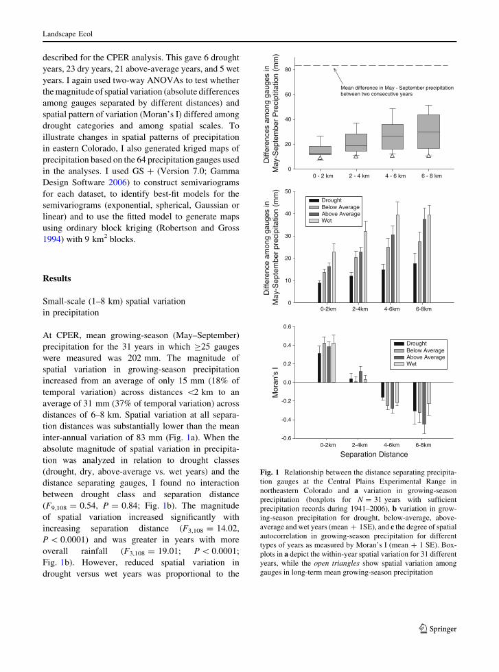
At CPER, mean growing-season (May–September)
precipitation for the 31 years in which C25 gauges
were measured was 202 mm. The magnitude of
spatial variation in growing-season precipitation
increased from an average of only 15 mm (18% of
temporal variation) across distances \2 km to an
average of 31 mm (37% of temporal variation) across
distances of 6–8 km. Spatial variation at all separa-
tion distances was substantially lower than the mean
inter-annual variation of 83 mm (Fig. 1a). When the
absolute magnitude of spatial variation in precipita-
tion was analyzed in relation to drought classes
(drought, dry, above-average vs. wet years) and the
distance separating gauges, I found no interaction
between drought class and separation distance
(F9,108 = 0.54, P = 0.84; Fig. 1b). The magnitude
of spatial variation increased significantly with
increasing separation distance (F3,108 = 14.02,
P \ 0.0001) and was greater in years with more
overall rainfall (F3,108 = 19.01; P \ 0.0001;
Fig. 1b). However, reduced spatial variation in
drought versus wet years was proportional to the
Diff
eren
ces
amon
g ga
uges
in
May
-Sep
tem
ber
Pre
cipt
itatio
n (m
m)
0
20
40
60
80
0 - 2 km 2 - 4 km 4 - 6 km 6 - 8 km
0-2km 2-4km 4-6km 6-8km
Diff
eren
ce a
mon
g ga
uges
in
May
-Sep
tem
ber
prec
ipita
tion
(mm
)
0
10
20
30
40
50
Drought Below Average Above Average Wet
Drought Below Average Above Average Wet
Separation Distance0-2km 2-4km 4-6km 6-8km
Mor
an's
I
-0.6
-0.4
-0.2
0.0
0.2
0.4
0.6
Mean difference in May - September precipitationbetween two consecutive years
Fig. 1 Relationship between the distance separating precipita-
tion gauges at the Central Plains Experimental Range in
northeastern Colorado and a variation in growing-season
precipitation (boxplots for N = 31 years with sufficient
precipitation records during 1941–2006), b variation in grow-
ing-season precipitation for drought, below-average, above-
average and wet years (mean ? 1SE), and c the degree of spatial
autocorrelation in growing-season precipitation for different
types of years as measured by Moran’s I (mean ? 1 SE). Box-
plots in a depict the within-year spatial variation for 31 different
years, while the open triangles show spatial variation among
gauges in long-term mean growing-season precipitation
Landscape Ecol
123
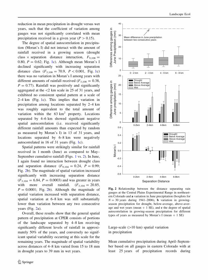
reduction in mean precipitation in drought versus wet
years, such that the coefficient of variation among
gauges was not significantly correlated with mean
precipitation received in a given year (P [ 0.15).
The degree of spatial autocorrelation in precipita-
tion (Moran’s I) did not interact with the amount of
rainfall received in a growing season (drought
class 9 separation distance interaction, F9,108 =
0.80, P = 0.62; Fig. 1c). Although mean Moran’s I
declined significantly with increasing separation
distance class (F3,108 = 70.9, P \ 0.001, Fig. 1c)
there was no variation in Moran’s I among years with
different amounts of rainfall received (F3,108 = 0.38,
P = 0.77). Rainfall was positively and significantly
aggregated at the\2 km scale in 25 of 31 years, and
exhibited no consistent spatial pattern at a scale of
2–4 km (Fig. 1c). This implies that variation in
precipitation among locations separated by 2–4 km
was roughly equivalent to the total amount of
variation within the 63 km2 property. Locations
separated by 4–6 km showed significant negative
spatial autocorrelation (i.e. received significantly
different rainfall amounts than expected by random
as measured by Moran’s I) in 13 of 31 years, and
locations separated by 6–8 km were negatively
autocorrelated in 16 of 31 years (Fig. 1c).
Spatial patterns were strikingly similar for rainfall
received in 1 month (June) as compared to May–
September cumulative rainfall (Figs. 1 vs. 2). In June,
I again found no interaction between drought class
and separation distance (F9,104 = 0.24, P = 0.99;
Fig. 2b). The magnitude of spatial variation increased
significantly with increasing separation distance
(F3,104 = 6.84, P = 0.0003) and was greater in years
with more overall rainfall. (F3,104 = 20.85,
P = 0.0001; Fig. 2b). Although the magnitude of
spatial variation increased with separation distance,
spatial variation at 6–8 km was still substantially
lower than variation between any two consecutive
years (Fig. 2a).
Overall, these results show that the general spatial
pattern of precipitation at CPER consists of portions
of the landscape separated by 4–8 km receiving
significantly different levels of rainfall in approxi-
mately 50% of the years, and conversely no signif-
icant spatial variability occurring at this scale for the
remaining years. The magnitude of spatial variability
across distances of 4–8 km varied from 15 to 18 mm
in drought years to 39 mm in wet years.
Large-scale ([10 km) spatial variation
in precipitation
Mean cumulative precipitation during April–Septem-
ber based on all gauges in eastern Colorado with at
least 25 years of precipitation records during
0 - 2 km 2 - 4 km 4 - 6 km 6 - 8 km
Diff
eren
ces
amon
g ga
uges
in
June
Pre
cipt
itatio
n (m
m)
0
10
20
30
40
Mean difference in June precipitationbetween two consecutive years
Diff
eren
ce a
mon
g ga
uges
in
June
pre
cipi
tatio
n (m
m)
0
5
10
15
20
25
Separation Distance
0-2km 2-4km 4-6km 6-8km
0-2km 2-4km 4-6km 6-8km
Mor
an's
I
-0.6
-0.4
-0.2
0.0
0.2
0.4
0.6
Drought Below Average Above Average Wet
Drought Below Average Above Average Wet
Fig. 2 Relationship between the distance separating rain
gauges at the Central Plains Experimental Range in northeast-
ern Colorado and a variation in June precipitation (boxplots for
N = 30 years during 1941–2006), b variation in growing-
season precipitation for drought, below-average, above-aver-
age and wet years (mean ? 1 SE), and c the degree of spatial
autocorrelation in growing-season precipitation for different
types of years as measured by Moran’s I (mean ? 1 SE)
Landscape Ecol
123
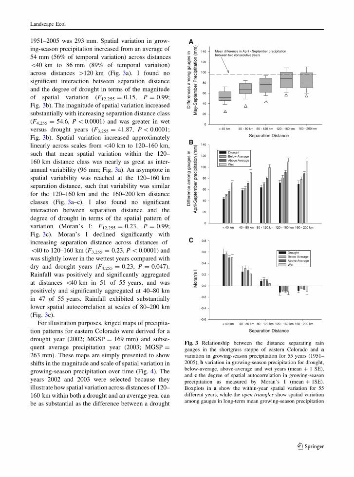
1951–2005 was 293 mm. Spatial variation in grow-
ing-season precipitation increased from an average of
54 mm (56% of temporal variation) across distances
\40 km to 86 mm (89% of temporal variation)
across distances [120 km (Fig. 3a). I found no
significant interaction between separation distance
and the degree of drought in terms of the magnitude
of spatial variation (F12,255 = 0.15, P = 0.99;
Fig. 3b). The magnitude of spatial variation increased
substantially with increasing separation distance class
(F4,255 = 54.6, P \ 0.0001) and was greater in wet
versus drought years (F3,255 = 41.87, P \ 0.0001;
Fig. 3b). Spatial variation increased approximately
linearly across scales from \40 km to 120–160 km,
such that mean spatial variation within the 120–
160 km distance class was nearly as great as inter-
annual variability (96 mm; Fig. 3a). An asymptote in
spatial variability was reached at the 120–160 km
separation distance, such that variability was similar
for the 120–160 km and the 160–200 km distance
classes (Fig. 3a–c). I also found no significant
interaction between separation distance and the
degree of drought in terms of the spatial pattern of
variation (Moran’s I: F12,255 = 0.23, P = 0.99;
Fig. 3c). Moran’s I declined significantly with
increasing separation distance across distances of
\40 to 120–160 km (F3,255 = 0.23, P \ 0.0001) and
was slightly lower in the wettest years compared with
dry and drought years (F4,255 = 0.23, P = 0.047).
Rainfall was positively and significantly aggregated
at distances \40 km in 51 of 55 years, and was
positively and significantly aggregated at 40–80 km
in 47 of 55 years. Rainfall exhibited substantially
lower spatial autocorrelation at scales of 80–200 km
(Fig. 3c).
For illustration purposes, kriged maps of precipita-
tion patterns for eastern Colorado were derived for a
drought year (2002; MGSP = 169 mm) and subse-
quent average precipitation year (2003; MGSP =
263 mm). These maps are simply presented to show
shifts in the magnitude and scale of spatial variation in
growing-season precipitation over time (Fig. 4). The
years 2002 and 2003 were selected because they
illustrate how spatial variation across distances of 120–
160 km within both a drought and an average year can
be as substantial as the difference between a drought
Diff
eren
ce a
mon
g ga
uges
in
Apr
il-S
epte
mbe
r pr
ecip
itatio
n (m
m)
0
20
40
60
80
100
120
140
Drought Below Average Above Average Wet
Separation Distance
Separation Distance
< 40 km 40 - 80 km 80 - 120 km 120 - 160 km 160 - 200 km
< 40 km 40 - 80 km 80 - 120 km 120 - 160 km 160 - 200 km
< 40 km 40 - 80 km 80 - 120 km 120 - 160 km 160 - 200 km
Mor
an's
I
-0.6
-0.4
-0.2
0.0
0.2
0.4
0.6
0.8
B
C
Diff
eren
ces
amon
g ga
uges
in
May
-Sep
tem
ber
Pre
cipt
itatio
n (m
m)
0
20
40
60
80
100
120
140 Mean difference in April - September precipitationbetween two consecutive years
A
Drought Below Average Above Average Wet
Fig. 3 Relationship between the distance separating rain
gauges in the shortgrass steppe of eastern Colorado and avariation in growing-season precipitation for 55 years (1951–
2005), b variation in growing-season precipitation for drought,
below-average, above-average and wet years (mean ? 1 SE),
and c the degree of spatial autocorrelation in growing-season
precipitation as measured by Moran’s I (mean ? 1SE).
Boxplots in a show the within-year spatial variation for 55
different years, while the open triangles show spatial variation
among gauges in long-term mean growing-season precipitation
Landscape Ecol
123
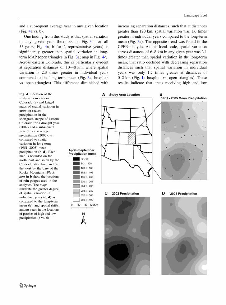
and a subsequent average year in any given location
(Fig. 4a vs. b).
One finding from this study is that spatial variation
in any given year (boxplots in Fig. 3a for all
55 years; Fig. 4a, b for 2 representative years) is
significantly greater than spatial variation in long-
term MAP (open triangles in Fig. 3a; map in Fig. 4c).
Across eastern Colorado, this is particularly evident
at separation distances of 10–40 km, where spatial
variation is 2.3 times greater in individual years
compared to the long-term mean (Fig. 3a, boxplots
vs. open triangles). This difference diminished with
increasing separation distances, such that at distances
greater than 120 km, spatial variation was 1.6 times
greater in individual years compared to the long-term
mean (Fig. 3a). The opposite trend was found in the
CPER analysis. At this local scale, spatial variation
across distances of 6–8 km in any given year was 3.1
times greater than spatial variation in the long-term
mean; that ratio declined with decreasing separation
distances such that spatial variation in individual
years was only 1.7 times greater at distances of
0–2 km (Fig. 1a boxplots vs. open triangles). These
results indicate that areas receiving high and low
Fig. 4 Location of the
study area in eastern
Colorado (a) and kriged
maps of spatial variation in
growing-season
precipitation in the
shortgrass-steppe of eastern
Colorado for a drought year
(2002) and a subsequent
year of near-average
precipitation (2003), as
compared to spatial
variation in long-term
(1951–2005) mean
precipitation (b–d). Each
map is bounded on the
north, east and south by the
Colorado state line, and on
the west by the base of the
Rocky Mountains. Blackdots in b show the locations
of rain gauges used in the
analyses. The mapsillustrate the greater degree
of spatial variation in
individual years (c, d) as
compared to the long-term
mean (b), and spatial shifts
among years in the locations
of patches of high and low
precipitation (c vs. d)
Landscape Ecol
123
levels of precipitation in any given year shift over
time (example in Fig. 4a vs. b).
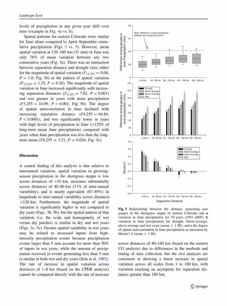
Spatial patterns for eastern Colorado were similar
for June alone compared to April–September cumu-
lative precipitation (Figs. 3 vs. 5). However, mean
spatial variation at 120–160 km (31 mm) in June was
only 76% of mean variation between any two
consecutive years (Fig. 5a). There was no interaction
between separation distance and drought class either
for the magnitude of spatial variation (F12,255 = 0.04,
P = 1.0; Fig. 5b) or the pattern of spatial variation
(F12,255 = 1.25, P = 0.26). The magnitude of spatial
variation in June increased significantly with increas-
ing separation distances (F4,255 = 7.92, P \ 0.001)
and was greater in years with more precipitation
(F3,255 = 16.09, P \ 0.001; Fig. 5b). The degree
of spatial autocorrelation in June declined with
increasing separation distance (F4,255 = 64.84,
P \ 0.0001), and was significantly lower in years
with high levels of precipitation in June ([125% of
long-term mean June precipitation) compared with
years when June precipitation was less than the long-
term mean (F4,255 = 3.21, P = 0.024; Fig. 5c).
Discussion
A central finding of this analysis is that relative to
interannual variation, spatial variation in growing-
season precipitation in the shortgrass steppe is low
across distances of \10 km, increases substantially
across distances of 40–80 km (71% of inter-annual
variability), and is nearly equivalent (87–89%) in
magnitude to inter-annual variability across distances
[120 km. Furthermore, the magnitude of spatial
variation is significantly higher in wet compared to
dry years (Figs. 3b, 5b), but the spatial pattern of that
variation (i.e. the scale and homogeneity of wet
versus dry patches) is similar in dry and wet years
(Figs. 3c, 5c). Greater spatial variability in wet years
may be related to increased inputs from high-
intensity precipitation events because precipitation
events larger than 5 mm account for more than 50%
of inputs in wet years, while the amount of precip-
itation received in events generating less than 5 mm
is similar in both wet and dry years (Sala et al. 1992).
The rate of increase in spatial variation across
distances of 1–8 km (based on the CPER analysis)
cannot be compared directly with the rate of increase
across distances of 40–160 km (based on the eastern
CO analysis) due to differences in the methods and
timing of data collection, but the two analyses are
consistent in showing a linear increase in spatial
variation across all scales from 1 to 160 km, with
variation reaching an asymptote for separation dis-
tances greater than 160 km.
Diff
eren
ces
amon
g ga
uges
in
June
Pre
cipt
itatio
n (m
m)
0
20
40
60
80
Mean difference in June precipitationbetween two consecutive years
Diff
eren
ce a
mon
g ga
uges
in
June
pre
cipi
tatio
n (m
m)
0
20
40
60
80
100
120
140
Drought Below Average Above Average Wet
Separation Distance
< 40 km 40 - 80 km 80 - 120 km 120 - 160 km 160 - 200 km
< 40 km 40 - 80 km 80 - 120 km 120 - 160 km 160 - 200 km
< 40 km 40 - 80 km 80 - 120 km 120 - 160 km 160 - 200 km
Mor
an's
I
-0.6
-0.4
-0.2
0.0
0.2
0.4
0.6
0.8
Drought Below Average Above Average Wet
Fig. 5 Relationship between the distance separating rain
gauges in the shortgrass steppe of eastern Colorado and avariation in June precipitation for 55 years (1951–2005), bvariation in June precipitation for drought, below-average,
above-average and wet years (mean ? 1 SE), and c the degree
of spatial autocorrelation in June precipitation as measured by
Moran’s I (mean ? 1 SE)
Landscape Ecol
123
The fact that the eastern CO analysis showed the
strongest positive autocorrelation at a scale of
10–40 km (indicating homogenous patches at this
scale relative to variation across all of eastern CO) is
consistent with the finding that significant negative
spatial autocorrelation occurs at scales of 6–8 km
within the CPER property in 50% of the years. In
other words, an area with a diameter of approxi-
mately 8 km will typically encompass a boundary
between two distinct patches of high versus low
precipitation in approximately 50% of the years. In
the remaining years, an area the size of CPER is
entirely contained within a patch of high or low
precipitation. When viewed at the scale of all of
eastern Colorado, these patches are most homoge-
nous at scales of 10–40 km. Patches of this size are
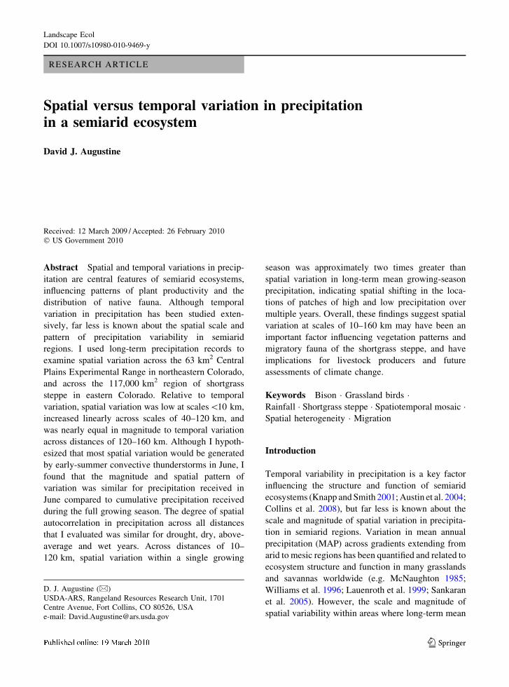
likely the result of inputs from intense, localized
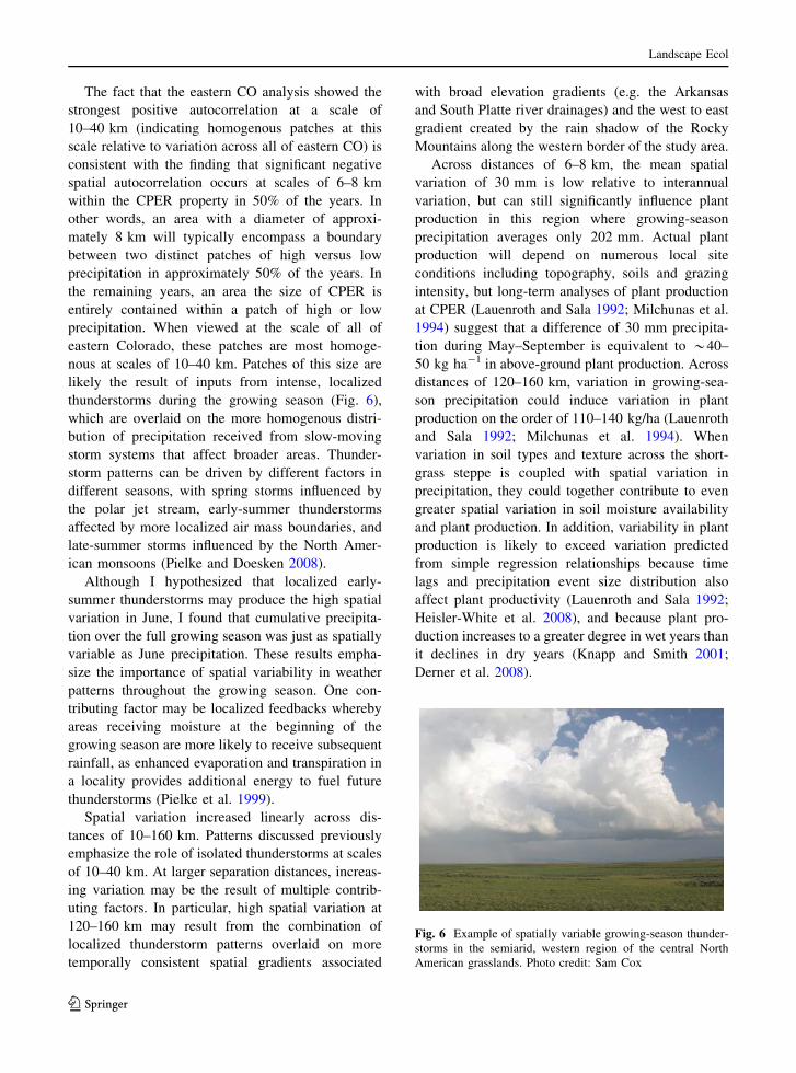
thunderstorms during the growing season (Fig. 6),
which are overlaid on the more homogenous distri-
bution of precipitation received from slow-moving
storm systems that affect broader areas. Thunder-
storm patterns can be driven by different factors in
different seasons, with spring storms influenced by
the polar jet stream, early-summer thunderstorms
affected by more localized air mass boundaries, and
late-summer storms influenced by the North Amer-
ican monsoons (Pielke and Doesken 2008).
Although I hypothesized that localized early-
summer thunderstorms may produce the high spatial
variation in June, I found that cumulative precipita-
tion over the full growing season was just as spatially
variable as June precipitation. These results empha-
size the importance of spatial variability in weather
patterns throughout the growing season. One con-
tributing factor may be localized feedbacks whereby
areas receiving moisture at the beginning of the
growing season are more likely to receive subsequent
rainfall, as enhanced evaporation and transpiration in
a locality provides additional energy to fuel future
thunderstorms (Pielke et al. 1999).
Spatial variation increased linearly across dis-
tances of 10–160 km. Patterns discussed previously
emphasize the role of isolated thunderstorms at scales
of 10–40 km. At larger separation distances, increas-
ing variation may be the result of multiple contrib-
uting factors. In particular, high spatial variation at
120–160 km may result from the combination of
localized thunderstorm patterns overlaid on more
temporally consistent spatial gradients associated
with broad elevation gradients (e.g. the Arkansas
and South Platte river drainages) and the west to east
gradient created by the rain shadow of the Rocky
Mountains along the western border of the study area.
Across distances of 6–8 km, the mean spatial
variation of 30 mm is low relative to interannual
variation, but can still significantly influence plant
production in this region where growing-season
precipitation averages only 202 mm. Actual plant
production will depend on numerous local site
conditions including topography, soils and grazing
intensity, but long-term analyses of plant production
at CPER (Lauenroth and Sala 1992; Milchunas et al.
1994) suggest that a difference of 30 mm precipita-
tion during May–September is equivalent to *40–
50 kg ha-1 in above-ground plant production. Across
distances of 120–160 km, variation in growing-sea-
son precipitation could induce variation in plant
production on the order of 110–140 kg/ha (Lauenroth
and Sala 1992; Milchunas et al. 1994). When
variation in soil types and texture across the short-
grass steppe is coupled with spatial variation in
precipitation, they could together contribute to even
greater spatial variation in soil moisture availability
and plant production. In addition, variability in plant
production is likely to exceed variation predicted
from simple regression relationships because time
lags and precipitation event size distribution also
affect plant productivity (Lauenroth and Sala 1992;
Heisler-White et al. 2008), and because plant pro-
duction increases to a greater degree in wet years than
it declines in dry years (Knapp and Smith 2001;
Derner et al. 2008).
Fig. 6 Example of spatially variable growing-season thunder-
storms in the semiarid, western region of the central North
American grasslands. Photo credit: Sam Cox
Landscape Ecol
123
Spatial variability in rainfall could have been one
factor affecting mobile fauna in this region prior to
European settlement. For example, one-way bison
migrations in Wyoming and Utah are on the order of
22–45 km (Berger 2004; Bruggeman et al. 2007) and
migratory movements [100 km are undertaken by
several other large ungulate species (Berger 2004).
Thus, bison movements in response to the substantial
spatial variation in precipitation that I documented at
scales of 40–160 km could clearly have been ener-
getically feasible. Movements in response to spatial
variability in forage resources can reduce the effect of
temporal variability on density-dependence in ungu-
late populations, as has been shown for elk and bison
populations in montane habitats (Wang et al. 2006).
Although field assessments of how spatial precipita-
tion variability affects on grazer movements are not
possible, spatially explicit ecosystem models that
simulate vegetation dynamics, ungulate foraging
decisions, and movement patterns (e.g. Christensen
et al. 2003; Plumb et al. 2009) may be an effective
means to explore the consequences of spatial precip-
itation patterns that I documented for large-scale
herbivore movement. Responses of migratory bird
populations to spatial variability in precipitation have
also been of considerable interest to ecologists
(Wiens 1974), and today have direct implications
for the design of grassland reserve networks. For
example, two smaller properties separated by
40–80 km experience more than twice the variation
in precipitation than a single large property. When
combined with information on how at-risk bird
species shift breeding locations among years, such
information can assist in the effective allocation of
conservation efforts.
Ranches on the order of 50–100 km2 can span
distances of 7–10 km, and ranches with separate
parcels can be distributed over even larger distances.
My findings concerning high spatial variability in
precipitation at scales of 120–160 km suggest that
movement of livestock over such distances through
collaborative networks of livestock producers may be
one means to mitigate temporal variation in precip-
itation. Recent discussions between U.S. and African
livestock producers have emphasized the value of
large-scale livestock mobility (Curtin and Western
2008), and such ‘agistment’ networks are most
effective where spatial variation in resource avail-
ability is high (McAllister et al. 2006). I also note that
the National Grasslands in the shortgrass steppe each
encompass *440–1800 km2 of public rangeland that
present substantial opportunities for large-scale shifts
in cattle stocking rates in response to spatially
variable precipitation patterns.
Another practical use of this analysis concerns the
reliability of using precipitation records from an off-
site weather station to represent a nearby, unmea-
sured location. While this will depend on the
application of the data, my analysis across spatial
scales of 1–8 km at CPER found that variation across
distances of as little as 2–4 km is similar in magni-
tude to variation across the entire 63 km2 property.
Where accurate measures of precipitation for a local
study are important, my results suggest gauges should
be within 2 km of the study site. At the same time,
the magnitude of variation across the 63 km2 prop-
erty was small compared to interannual variability, so
for some applications, using measurements from a
single gauge may be reasonably reliable for distances
up to 8 km away. Beyond this, the potential differ-
ence in precipitation between a gauge and an
unmeasured location increases linearly up to a
separation distance of 160 km (Fig. 3a).
Within the expansive and topographically homog-
enous shortgrass steppe, my analysis emphasizes the
importance of spatially variable precipitation at all
scales. In particular, spatial variation is equivalent in
magnitude to inter-annual variation at scales of 120–
160 km. Management and conservation strategies for
semiarid rangelands can be increasingly effective by
recognizing and incorporating this source of spatial
variation.
Acknowledgements I thank Mary Ashby and Jeff Thomas
for their dedication in collecting and maintaining the long-term
precipitation data at CPER. I thank Drs. Justin Derner, Daniel
Milchunas, Nolan Doeskan, and two anonymous reviewers for
comments that greatly improved the manuscript, and Dr. Mark
West for assistance with scripts to calculate Moran’s I using
the statistical package R.
References
Austin AT, Yahdjian L, Stark JM, Belnap J, Porporato A,
Norton U, Ravetta DA, Schaeffer SM (2004) Water pulses
and biogeochemical cycles in arid and semiarid ecosys-
tems. Oecologia 141:221–235
Bamforth D (1987) Historical documents and bison ecology on
the Great Plains. Plains Anthropol 32:1–15
Landscape Ecol
123
Berger J (2004) The last mile: how to sustain long-distance
migration in mammals. Conserv Biol 18:320–331
Brennan L, Kuvleskey W (2005) North American grassland
birds: an unfolding conservation crisis? J Wildl Manage
69:1–13
Bruggeman JE, Garrott RA, White PJ, Watson FGR, Wallen R
(2007) Covariates affecting spatial variability in bison
travel behavior in Yellowstone National Park. Ecol Appl
17:1411–1423
Christensen JH, Hewiston B (2007) Regional climate projec-
tions. In: Solomin S, Qin D, Manning M, Chen Z, Marquis
KB, Averyt M, Tignor M, Miller HL (eds) Climate change
2007: The physical science basis. Contribution of Work-
ing Group I to the Fourth Assessment Report of the
Intergovernmental Panel on Climate Change. Cambridge
University Press, New York, NY, USA, pp 849–926, 11
March 2009. http://www.ipcc.ch/pdf/assessment-report/
ar4/wg1/ar4-wg1-chapter11.pdf
Christensen L, Coughenour MB, Ellis JE, Chen Z (2003)
Sustainability of inner Mongolian grasslands: application
of the Savanna model. J Range Manage 56:319–327
Collins SL, Sinsabaugh RL, Crenshaw C, Green L, Porras-
Alfaro A, Stursova M, Zeglin LH (2008) Pulse dynamics
and microbial processes in aridland ecosystems. J Ecol
96:413–420
Coughenour M (1991) Spatial components of plant-herbivore
interactions in pastoral, ranching, and native ungulate
ecosystems. J Range Manage 44:530–542
Curtin C, Western D (2008) Grasslands, people, and conser-
vation: over-the-horizon learning exchanges between
African and American pastoralists. Conserv Biol 22:870–
877
Derner JD, Hess BW, Olson RA, Schuman GE (2008) Func-
tional group and species responses to precipitation in three
semi-arid rangeland ecosystems. Arid Land Res Manage
22:81–92
Gamma Design Software (2006) GS ? Geostatistics for the
environmental sciences, Version 7.0. Gamma Design
Software, Plainwell, MI
Hart R (2001) Where the buffalo roamed—or did they? Great
Plains Res 11:83–102
Heisler-White JL, Knapp AK, Kelly EF (2008) Increasing
precipitation event size increases aboveground net pri-
mary productivity in a semi-arid grassland. Oecologia
158:129–140
Hubbard KG (1994) Spatial variability of daily weather vari-
ables in the high plains of the USA. Agric For Meteorol
68:29–41
Knapp AK, Smith MD (2001) Variation among biomes in
temporal dynamics of aboveground primary production.
Science 291:481–484
Lauenroth W, Milchunas D (1992) Short-grass steppe. In:
Coupland R (ed) Ecosystems of the world. Elsevier, New
York, NY, pp 183–226
Lauenroth WK, Sala OE (1992) Long-term forage production of
North American shortgrass steppe. Ecol Appl 2:397–403
Lauenroth WK, Burke IC, Gutmann MP (1999) The structure
and function of ecosystems in the central North American
grassland region. Great Plains Res 9:223–260
Legendre P, Fortin M (1989) Spatial pattern and ecological
analysis. Vegetatio 80:107–138
Lott D (2002) American bison: a natural history. University of
California Press, Berkeley, CA
McAllister R, Gordon I, Janssen M, Abel N (2006) Pastoralists
responses to variation of rangeland resources in time and
space. Ecol Appl 16:572–583
McNaughton SJ (1985) Ecology of a grazing ecosystem: the
Serengeti. Ecol Monogr 55:259–294
Meehl GA, Stocker TF, Collins WD, Friedlingstein P, Gaye
AT, Gregory JM, Kitoh A, Knutti R, Murphy J, Noda A,
Raper SCB, Watterson IG, Weaver AJ, Zhao ZC (2007)
Global climate projections. In: Solomon S, Qin D, Man-
ning M, Chen Z, Marquis M, Averyt KB, Tignor M,
Miller HL (eds) Climate change 2007: the physical sci-
ence basis. Contribution of Working Group I to the Fourth
Assessment Report of the Intergovernmental Panel on
Climate Change. Cambridge University Press, New York,
NY, USA, pp 749–844, 11 March 2009. http://www.ipcc.
ch/pdf/assessment-report/ar4/wg1/ar4-wg1-chapter10.pdf
Milchunas DG, Lauenroth WK, Chapman PL, Kazempour MK
(1989) Effects of grazing, topography and precipitation on
the structure of a semiarid grassland. Vegetatio 80:11–23
Milchunas DG, Forwood J, Lauenroth WK (1994) Productivity
of long-term grazing treatments in response to seasonal
precipitation. J Range Manage 47:133–139
Milchunas DG, Laurenroth WK, Burke IC (1998) Livestock
grazing: animal and plant biodiversity of shortgrass steppe
and the relationship to ecosystem function. Oikos 83:65–
74
Pielke RA, Doesken N (2008) Climate of the shortgrass steppe.
In: Lauenroth W, Burke I (eds) Ecology of the shortgrass
steppe. Oxford University Press, New York, pp 14–29
Pielke RA, Liston GE, Eastman JL, Lu L, Coughenour M
(1999) Seasonal weather prediction as an initial value
problem. J Geophys Res D 104:19463–19479
Plumb GE, White PJ, Coughenour MB, Wallen RL (2009)
Carrying capacity, migration, and dispersal in Yellow-
stone bison. Biol Conserv 142:2377–2387
Robertson GP, Gross KL (1994) Assessing the heterogeneity of
below-ground resources: quantifying pattern and scale. In:
Caldwell MM, Pearcy RW (eds) Plant exploitation of
environmental heterogeneity. Academic Press, New York,
pp 237–253
Sala O, Lauenroth W (1982) Small rainfall events: an eco-
logical role in semiarid regions. Oecologia 53:301–304
Sala OE, Lauenroth WK, Parton WJ (1992) Long-term soil
water dynamics in the shortgrass steppe. Ecology
73:1175–1181
Samson FB, Knopf FL, Ostlie WR (2004) Great Plains eco-
systems: past, present and future. Wildl Soc Bull 32:6–15
Sankaran M, Hanan NP, Scholes RJ, Ratnam J, Augustine DJ,
Cade BS, Gignoux J, Higgins SI, Le Roux X, Ludwig F,
Ardo J, Banyikwa F, Bronn A, Bucini G, Caylor KK,
Coughenour MB, Diouf A, Ekaya W, Feral CJ, February
EC, Frost PGH, Hiernaux P, Hrabar H, Metzger KL, Prins
HHT, Ringrose S, Sea W, Tews J, Worden J, Zambatis N
(2005) Determinants of woody cover in African savannas.
Nature 438:846–849
Sokal R, Oden N (1978) Spatial autocorrelation in biology 2.
Some biological implications and four applications of
evolutionary and ecological interest. Biol J Linn Soc
10:229–249
Landscape Ecol
123

Wang G, Hobbs N, Boone R, Illius A, Gordon I, Gross J,
Hamlin K (2006) Spatial and temporal variability modify
density dependence in populations of large herbivores.
Ecology 87:95–102
Wiens J (1972) Predictability of patterns and variability of
precipitation at IBP Grassland Biome sites. US IBP
Grassland Biome, Technical Report #168, Colorado State
University, Fort Collins, CO, USA
Wiens J (1974) Climatic instability and the ‘‘ecological satu-
ration’’ of bird communities in North American grass-
lands. Condor 76:385–400
Williams R, Duff G, Bowman D, Cook G (1996) Variation in
the composition and structure of tropical savannas as a
function of rainfall and soil texture along a large-scale
climatic gradient in the Northern Territory, Australia. J
Biogeogr 23:747–756
Landscape Ecol
123