Spatial Analysis

Longley et al., Ch 14,15

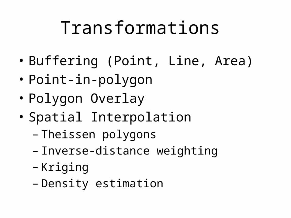
Transformations

• Buffering (Point, Line, Area)

• Point-in-polygon

• Polygon Overlay

• Spatial Interpolation– Theissen polygons– Inverse-distance weighting– Kriging– Density estimation

Basic Approach

Map

Transformation

New map

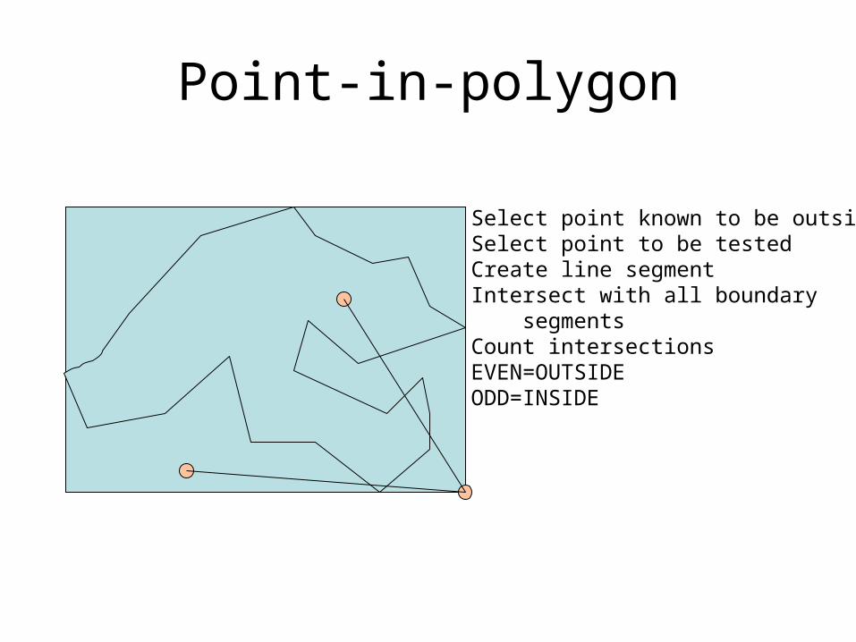
Point-in-polygon

Select point known to be outsideSelect point to be testedCreate line segmentIntersect with all boundary segmentsCount intersectionsEVEN=OUTSIDEODD=INSIDE

Create a buffer: Raster

Create a Buffer: vector

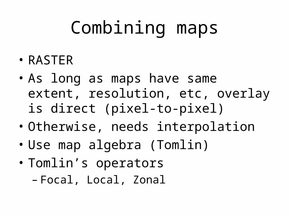
Combining maps

• RASTER

• As long as maps have same extent, resolution, etc, overlay is direct (pixel-to-pixel)

• Otherwise, needs interpolation

• Use map algebra (Tomlin)

• Tomlin’s operators– Focal, Local, Zonal

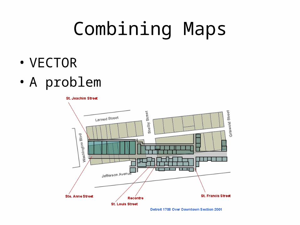
Combining Maps

• VECTOR

• A problem

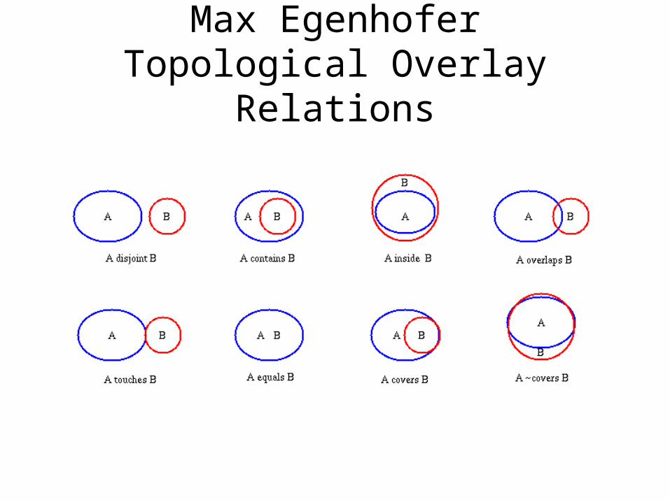
Max EgenhoferTopological Overlay Relations

Creating new zones

Town buffer

River buffer

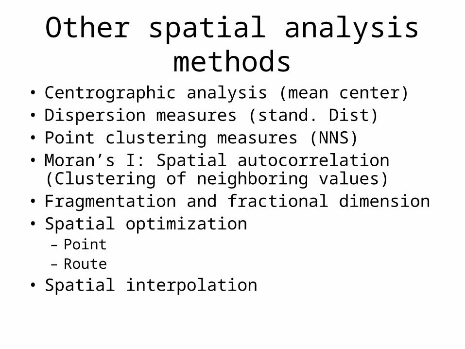
Other spatial analysis methods

• Centrographic analysis (mean center)• Dispersion measures (stand. Dist)• Point clustering measures (NNS)• Moran’s I: Spatial autocorrelation (Clustering of

neighboring values)• Fragmentation and fractional dimension• Spatial optimization

– Point– Route

• Spatial interpolation

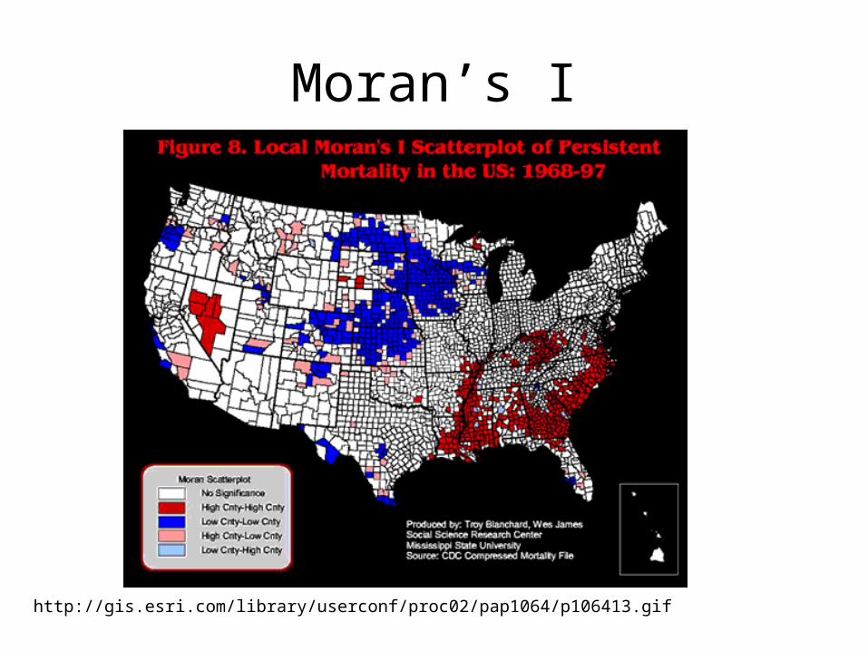
Moran’s I

http://gis.esri.com/library/userconf/proc02/pap1064/p106413.gif

Spatial autocorrelation

• Correlation of a field with itself

Low

High

Maximum

Spatial optimization

www.giscenter.net/eng/work_03_e.html

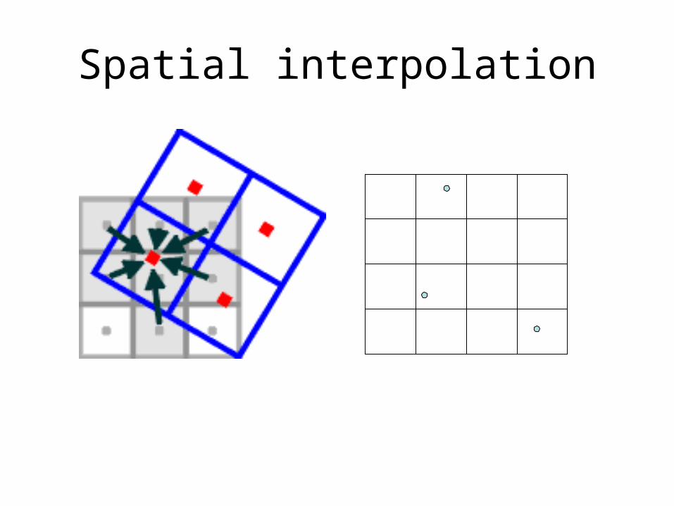
Spatial interpolation

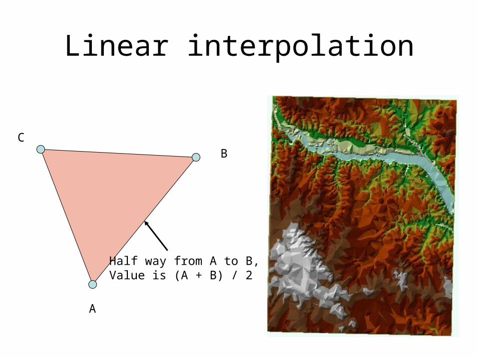
Linear interpolation

Half way from A to B,Value is (A + B) / 2

A

BC

Nonlinear Interpolation

• When things aren't or shouldn’t be so simple• Values computed by piecewise “moving

window”• Basic types:

1. Trend surface analysis / Polynomial

2. Minimum Curvature Spline

3. Inverse Distance Weighted 4. Kriging

1. Trend Surface/Polynomial

• point-based • Fits a polynomial to input points• When calculating function that will

describe surface, uses least-square regression fit

• approximate interpolator– Resulting surface doesn’t pass through all

data points– global trend in data, varying slowly overlain

by local but rapid fluctuations

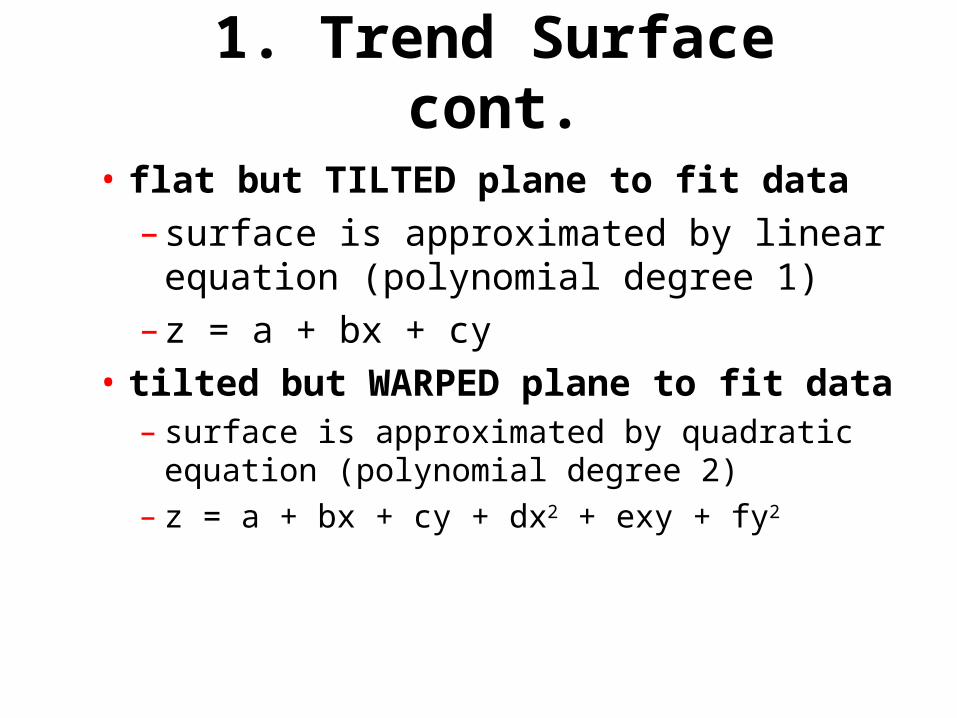
1. Trend Surface cont.

• flat but TILTED plane to fit data

– surface is approximated by linear equation (polynomial degree 1)

– z = a + bx + cy

• tilted but WARPED plane to fit data– surface is approximated by quadratic

equation (polynomial degree 2)– z = a + bx + cy + dx2 + exy + fy2

Trend Surfaces

2. Minimum Curvature Splines

• Fits a minimum-curvature surface through input points

• Like bending a sheet of rubber to pass through points– While minimizing curvature of that sheet

• repeatedly applies a smoothing equation (piecewise polynomial) to the surface – Resulting surface passes through all points

• best for gently varying surfaces, not for rugged ones (can overshoot data values)

3. Distance Weighted Methods

• Each input point has local influence that diminishes with distance

• estimates are averages of values at n known points within window R

3. Inverse Distance Weighted

where w is some function of distance (e.g., w = 1/dk)

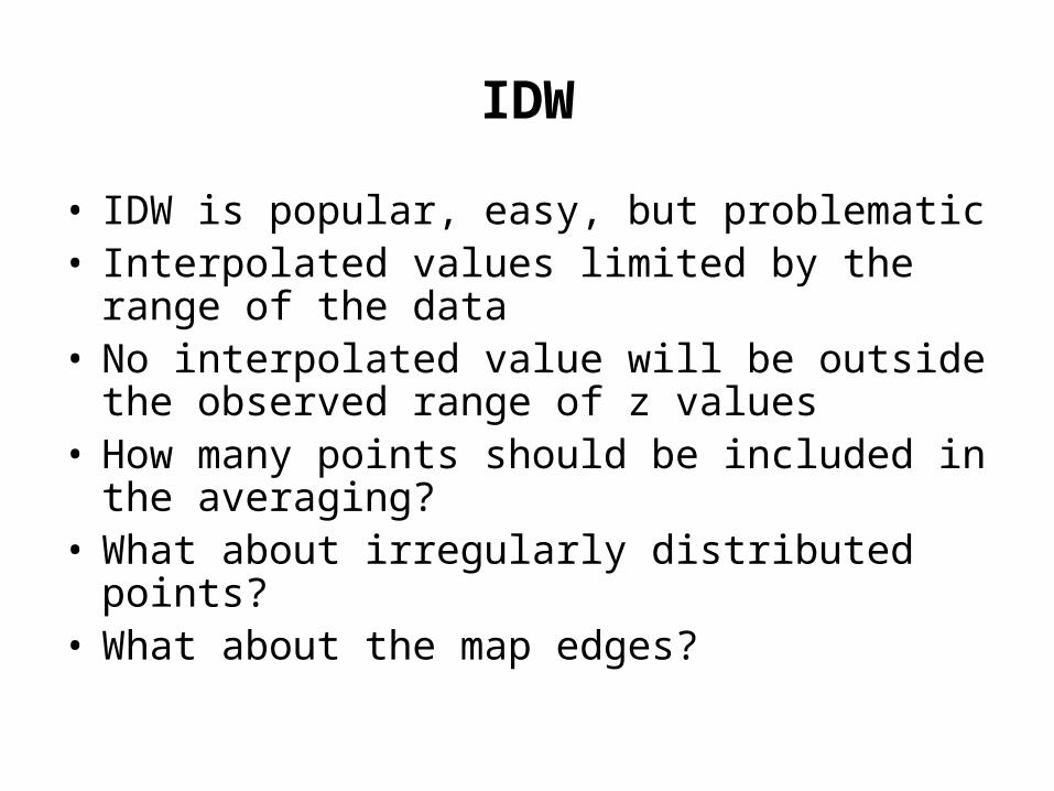
IDW

• IDW is popular, easy, but problematic • Interpolated values limited by the range of the

data• No interpolated value will be outside the

observed range of z values• How many points should be included in the

averaging? • What about irregularly distributed points?• What about the map edges?

IDW Example

• ozone concentrations at CA measurement stations

1. estimate a complete field, make a map

2. estimate ozone concentrations at specific locations (e.g., Los Angeles)

Ozone in S. Cal: Text Example

measuring stations and concentrations (point shapefile) CA cities (point shapefile) CA outline (polygon shapefile) DEM (raster)

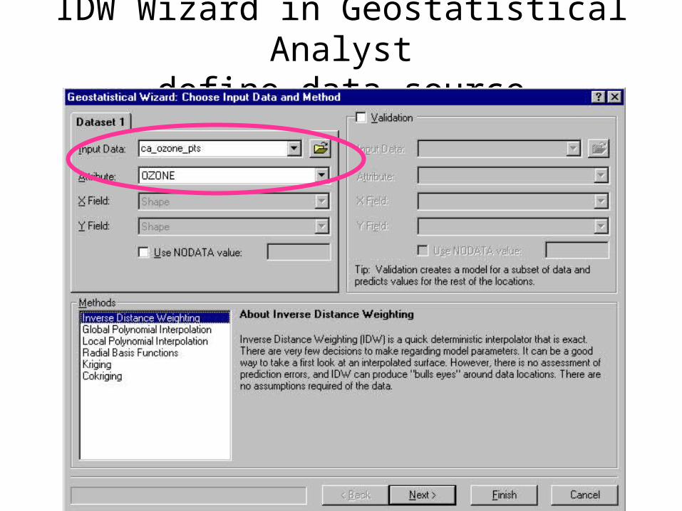
IDW Wizard in Geostatistical Analystdefine data source

Further define interpolation method

Power of distance

4 sectors

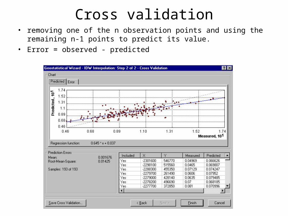
Cross validation• removing one of the n observation points and using the remaining n-1

points to predict its value.• Error = observed - predicted

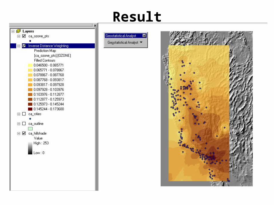
Result

4. Kriging

• Assumes distance or direction betw. sample points shows a spatial correlation that help describe the surface

• Fits function to – Specified number of points OR– All points within a window of specified radius

• Based on an analysis of the data, then an application of the results of this analysis to interpolation

• Most appropriate when you already know about spatially correlated distance or directional bias in data

• Involves several steps– Exploratory statistical analysis of data– Variogram modeling– Creating the surface based on variogram

Kriging

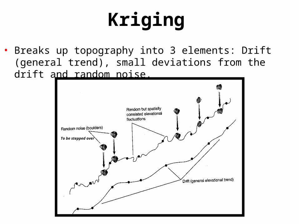
• Breaks up topography into 3 elements: Drift (general trend), small deviations from the drift and random noise.

To be stepped over

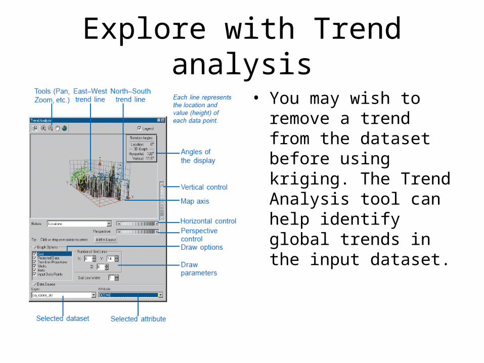
Explore with Trend analysis

• You may wish to remove a trend from the dataset before using kriging. The Trend Analysis tool can help identify global trends in the input dataset.

Kriging Results

• Once the variogram has been developed, it is used to estimate distance weights for interpolation

• Computationally very intensive w/ lots of data points

• Estimation of the variogram complex– No one method is absolute best– Results never absolute, assumptions about

distance, directional bias

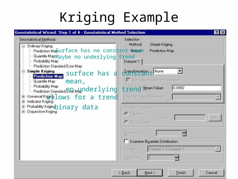
Kriging Example

Surface has no constant meanMaybe no underlying trend

surface has a constant mean, no underlying trend

binary data

allows for a trend

Analysis of Variogram

Fitting a Model, Directional Effects

How Many Neighbors?

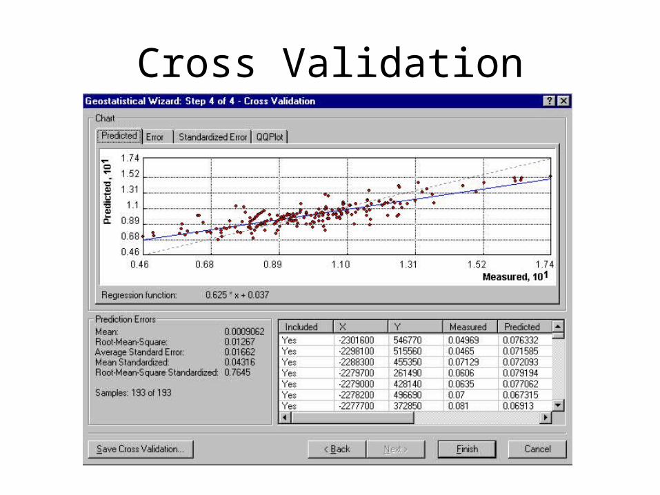
Cross Validation

Kriging Result• similar pattern to IDW• less detail in remote

areas • smooth

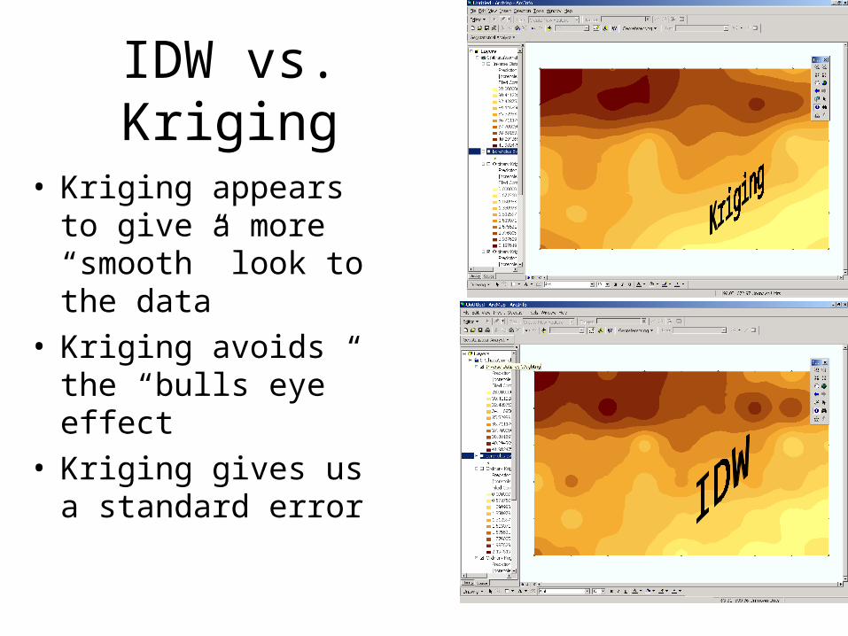
IDW vs. Kriging

• Kriging appears to give a more “smooth” look to the data

• Kriging avoids the “bulls eye” effect

• Kriging gives us a standard error