PHYSICAL REVIEW E 97, 032317 (2018)

Sparse dynamical Boltzmann machine for reconstructing complex networks with binary dynamics

Yu-Zhong Chen1 and Ying-Cheng Lai1,2,*

1School of Electrical, Computer and Energy Engineering, Arizona State University, Tempe, Arizona 85287, USA2Department of Physics, Arizona State University, Tempe, Arizona 85287, USA

(Received 7 April 2017; revised manuscript received 9 August 2017; published 28 March 2018)

Revealing the structure and dynamics of complex networked systems from observed data is a problem ofcurrent interest. Is it possible to develop a completely data-driven framework to decipher the network structureand different types of dynamical processes on complex networks? We develop a model named sparse dynamicalBoltzmann machine (SDBM) as a structural estimator for complex networks that host binary dynamical processes.The SDBM attains its topology according to that of the original system and is capable of simulating the originalbinary dynamical process. We develop a fully automated method based on compressive sensing and a clusteringalgorithm to construct the SDBM. We demonstrate, for a variety of representative dynamical processes on modeland real world complex networks, that the equivalent SDBM can recover the network structure of the originalsystem and simulates its dynamical behavior with high precision.

DOI: 10.1103/PhysRevE.97.032317

I. INTRODUCTION

A central issue in complexity science and engineering is sys-tems identification and dynamical behavior prediction based onexperimental or observational data. For a complex networkedsystem, often the network structure and the nodal dynamicalprocesses are unknown but only time series measured fromvarious nodes in the network can be obtained. The challengingtask is to infer the detailed network topology and the nodaldynamical processes from the available data. This line ofpursuit started in biomedical science for problems such asidentification of gene regulatory networks from expressiondata in systems biology [1–4] and uncovering various func-tional networks in the human brain from activation data inneuroscience [5–8]. The inverse problem has also been anarea of research in statistical physics where, for example, theinverse Ising problem in static [9–13] and kinetic [14–20]situations has attracted continuous interest. Recent years havewitnessed the emergence and growth of a subfield of researchin complex networks: data based network identification (orreverse engineering of complex networks) [21–35]. In theseworks, the success of mapping out the entire network structureand estimating the nodal dynamical equations partly relies ontaking advantage of the particular properties of the systemdynamics in terms of the specific types and rules. For exam-ple, depending on the detailed dynamical processes such ascontinuous-time oscillations [26,30–33,36,37], evolutionarygames [27], or epidemic spreading [28], appropriate mathe-matical frameworks uniquely tailored at the specific underlyingdynamical process can be formulated to solve the inverseproblem.

In this paper, we address the following challenging ques-tion: Is it possible to develop a completely data-driven frame-work for extracting the network topology and identifying

*ying-cheng.lai@asu.edu

the dynamical processes, without the need to know a priorithe specific types of network dynamics? An answer to thisquestion would be of significant value not only to complexityscience and engineering, but also to modern data science wherethe goal is to unearth the hidden structural information andto predict the future evolution of the system. We introducea Boltzmann machine for complex networked systems withpairwise interactions and demonstrate that such a “machine”can indeed be developed for a large number of distinct types ofbinary network dynamical processes. Our approach will be acombination of numerical computation and physical reasoning.Since we are yet able to develop a rigorous mathematicalframework, this work should be regarded as an initial attempttowards the development of a general framework for networkreconstruction and dynamics prediction.

The key principle underlying our work is the following. Inspite of the difference among the types of binary dynamics interms of, e.g., the interaction patterns and state updating rules,there are two common features shared by many dynamicalprocesses on complex networks: (1) they are stochastic, first-order Markovian processes, i.e., only the current state of thesystem determines its immediate future; and (2) the nodalinteractions are local, i.e., a node typically interacts with itsneighboring nodes, not all the nodes in the network. Thetwo features are characteristic of a Markov network (or aMarkov random field) [38,39]. In particular, a Markov networkis an undirected and weighted probabilistic graphical modelthat is effective for determining the complex probabilisticinterdependencies in situations where the directionality in theinteraction between the connected nodes cannot be naturallyassigned, in contrast to the directed Bayesian networks [38,39].In this work, however, we demonstrate that we can makea proper modification to the undirected Markov network toaccommodate networked systems with a directed topology.Note that a Markov network has two types of parameters: anodal bias parameter that controls its preference of the statechoice and a weight parameter characterizing the interaction

2470-0045/2018/97(3)/032317(21) 032317-1 ©2018 American Physical Society

YU-ZHONG CHEN AND YING-CHENG LAI PHYSICAL REVIEW E 97, 032317 (2018)

strength of each undirected link. In our work, the weightparameter of an incoming (or outgoing) link is defined tocharacterize the interaction from (or to) a neighboring nodein a directed network.

For a network of N nodes with xj being the state ofnode j (j = 1, . . . ,N), the joint probability distribution ofthe state variables X = (x1,x2, . . . ,xN )T is given by P (X) =∏

C φ(XC)/∑

X

∏C φ(XC), whereφ(XC) is the potential func-

tion for a well-connected network clique C, and the summationin the denominator is over all possible system state X. Ifthis joint probability distribution is available, all conditionalprobability interdependencies can be obtained. The way todefine a clique and to determine its potential function playsa key role in the Markov network’s representation power ofmodeling the interdependencies within a particular system.

To be concrete, in this work we pursue the possibility ofmodeling the conditional probability interdependencies of avariety of binary dynamical processes on complex networkedsystems via a properly modified Ising-Markov network withits potential function having the form of the Boltzmann factor,exp(−E), where E is the energy determined by the local statesand their interactions along with the network parameters (theincoming link weights and node biases) in a log-linear form[40]. This is effectively a sparse Boltzmann machine [40]that allows directed connections adopted to complex networktopologies without hidden units. (Note that hidden units usuallyplay a crucial role in ordinary Boltzmann machines [40].)We introduce a temporal evolution mechanism as a persistentsampling process for such a machine based on the conditionalprobabilities obtained via the joint probability, and generate aMarkov chain of persistently sampled state configurations toform the state transition time series for each node. We call ourmodel a sparse dynamical Boltzmann machine (SDBM).

For a binary dynamical process on complex networks,such as epidemic spreading or evolutionary game dynamics,the state of each node at the next time step is determinedby the probability conditioned on the current states of itsneighbors (and its own state in some cases). There is freedom tomanipulate the conditional probabilities that dictate the systembehavior in the immediate future through the adjustment of itsparameter values, i.e., the weights and biases. A basic questionis then, for an SDBM, is it possible to properly choose theseparameters so that the conditional probabilities so producedare approximately identical to those of the network dynamicalprocess with each given observed system state configuration? Ifthe answer is affirmative, the SDBM can serve as a dynamicsapproximator of the original system, and the approximatedconditional probabilities possess predictive power for thesystem state at the next time step. When such an SDBM is foundfor many types of dynamical process on complex networks ofvarious directed and undirected topologies, it effectively servesas a dynamics approximator.

When an approximator has been found for the dynamics on acomplex network, the topology of the SDBM is an approximaterepresentation of the original network, providing a solutionto the problem of network structure reconstruction. Previousworks on the inverse static or kinetic Ising problems led tomethods of reconstruction for Ising dynamics by maximizingthe data likelihood (or pseudolikelihood) function via variousgradient descent approaches [9–20]. Instead of adopting these

methods, as a part of our methodology to extract the networkstructure, we articulate a compressive sensing [41–46] basedapproach, whose working power has been demonstrated for avariety of non-Ising type of dynamics on complex networks[26–29,47–49]. By incorporating the K-means clustering al-gorithm into the sparse solution obtained from compressivesensing, we demonstrate that nearly perfect reconstruction ofthe complex network topology can be achieved. Using 14 dif-ferent types of dynamical processes on complex networks, wefind that, if the time series data generated by these dynamicalprocesses are assumed to be from its equivalent SDBMs, thereconstruction framework is capable of recovering the under-lying network structure for each type of original dynamicswith essentially zero error. This represents solid and concreteevidence that SDBM is capable of serving as a structuralestimator for complex networks with directed and undirectedinteractions. In addition to being able to precisely reconstructthe network topology, the SDBM also allows the link weightsand nodal biases to be calculated with high accuracy. Anappealing feature of our method is that it is fully automatedand does not require any subjective parameter choice.

Section II provides a general formulation of SDBM asa structural estimator with a focus on undirected networks.The use of compressive sensing and the implementation ofK-means algorithm are described. A parameter estimationscheme and a degree guided solution strategy are introduced.The issue of estimating link weights and nodal bias isaddressed. Section III presents reconstruction results for avariety of model and real networks coupled with 14 differenttypes of dynamical processes. Section IV contains a generaldiscussion of the SDBM method. A number of side issuestogether with certain details of the real networks are placed inthe Appendices.

II. METHOD FORMULATION

A. SDBM as a structural estimatorfor undirected complex networks

1. Sparse dynamical Boltzmann machine and compressive sensing

An SDBM with symmetric link weights is effectively aclassical Markov network. For an SDBM of size N , theprobability that the system is in a particular binary stateconfiguration XN×1 = (x1,x2, . . . ,xN )T is given by

P (X) = exp(−EX)∑X exp(−EX)

, (1)

where EX is the total energy of the network in X:

EX = XT · W · X =∑i �=j

wij xixj +N∑

i=1

bixi, (2)

xi and xj are binary variables (0 or 1) characterizing the statesof nodes i and j , respectively, and W is a weighted matrixwith its off diagonal elements wij = wji (i,j = 1, . . . ,N, i �=j ) specifying the weight associated with the link betweennodes i and j . The ith diagonal element of W is the biasparameter bi for node i (i = 1, . . . ,N), which determines nodei’s preference to state 0 or 1. The total energy EX includesthe interaction energies (the sum of all wijxixj terms) and

032317-2

SPARSE DYNAMICAL BOLTZMANN MACHINE FOR … PHYSICAL REVIEW E 97, 032317 (2018)

the nodes’ self-energies (the various bixi terms). The partitionfunction of the system is given by

Z =∑

X

exp(−EX), (3)

where the summation is over all possible X configurations.The state of node i at the next time step is determined by thestates of all other nodes at the present time step XR

i throughthe following conditional probability:

P{xi(t + 1) = 1

∣∣XRi (t)

} = P{xi(t + 1) = 1,XR

i (t)}

P{xi(t + 1) = 1,XR

i (t)} + P

{xi(t + 1) = 0,XR

i (t)} , (4)

where the two joint probabilities are given by

P{xi(t + 1) = 1,XR

i (t)} = 1

Z exp

⎡⎣−

N∑j=1,j �=i

wij xj (t) − bi −N∑

s=1,s �=i

N∑j=1,j �=i

wsj xs(t)xj (t) −N∑

s=1,s �=i

bsxs(t)

⎤⎦,

P{xi(t + 1) = 0,XR

i (t)} = 1

Z exp

⎡⎣−

N∑s=1,s �=i

N∑j=1,j �=i

wsj xs(t)xj (t) −N∑

s=1,s �=i

bsxs(t)

⎤⎦.

A Markov network defined in this fashion is in fact the kinetic Ising model [14–20]. With the joint probabilities, the conditionalprobability in Eq. (4) becomes

P{xi(t + 1) = 1

∣∣XRi (t)

} = 1

1 + exp[∑N

j=1,j �=i wij xj (t) + bi

] . (5)

We thus have

ln

(1

P{xi(t + 1) = 1

∣∣XRi (t)

} − 1

)=

N∑j=1,j �=i

wij xj (t) + bi.

Letting Qi(t) ≡ (P {xi(t + 1) = 1|XRi (t)})−1 − 1, we have

ln Qi(t) = (x1(t), . . . , xi−1(t), xi+1(t), . . . , xN (t), 1)

⎛⎜⎜⎜⎜⎜⎜⎜⎜⎜⎝

wi1...

wi(i−1)

wi(i+1)...

wiN

bi

⎞⎟⎟⎟⎟⎟⎟⎟⎟⎟⎠

. (6)

For M distinct time steps t1,t2, . . . ,tM , we obtain the following matrix form:

⎛⎜⎜⎝

ln Qi(t1)ln Qi(t2)

...ln Qi(tM )

⎞⎟⎟⎠ =

⎛⎜⎜⎝

x1(t1), . . . , xi−1(t1), xi+1(t1), . . . , xN (t1), 1x1(t2), . . . , xi−1(t2), xi+1(t2), . . . , xN (t2), 1

......

......

......

...x1(tM ), . . . , xi−1(tM ), xi+1(tM ), . . . , xN (tM ), 1

⎞⎟⎟⎠

⎛⎜⎜⎜⎜⎜⎜⎜⎜⎜⎝

wi1...

wi(i−1)

wi(i+1)...

wiN

bi

⎞⎟⎟⎟⎟⎟⎟⎟⎟⎟⎠

, (7)

which can be written concisely as

YM×1 = �M×N · VN×1, (8)

where the vector YM×1 ∈ RM contains the values of ln Qi(t)for M different time steps, the M × N matrix �M×N isdetermined by the states of all the nodes except i, and the first(N − 1) components of the vector VN×1 ∈ RN are the linkweights between node i and all other nodes in the network, asillustrated in Fig. 1, with its last entry being node i’s intrinsicbias.

Since the conditional probability P {xi(t + 1) = 1|XRi (t)}

depends solely on the state configuration of i’s nearestneighbors, or i’s Markov blanket [38,39] at time t , as shownin Fig. 1(b), identical configurations at other time steps implyidentical conditional probabilities. Thus, given time series dataof the dynamical process, the conditional probability can beestimated according to the law of large numbers by averagingover the states of i at all the time steps prior to the neighboringstate configurations becoming identical. Note, however,that this probability needs to be conditioned on the state

032317-3

YU-ZHONG CHEN AND YING-CHENG LAI PHYSICAL REVIEW E 97, 032317 (2018)

configuration of the entire system except node i, i.e., on XRi (t),

and the average of xi is calculated over all the time steps tm + 1satisfying XR

i (t) = XRi (tm). This means that there can be a

dramatic increase in the configuration size, i.e., from ki (the de-gree of node i) to N − 1 (the size of the vector XR

i ), which canmake the number of exactly identical configurations too small

to give any meaningful statistics. To overcome this difficulty,we allow a small amount of dissimilarity between XR

i (t) andXR

i (tm) by introducing a tolerance parameter � (0 � � � 0.5)to confine the corresponding Hamming distances normalizedby N . In particular, we assume XR

i (t) ≈ XRi (tm) if the relative

difference between them is not larger than �. This averagingprocess leads to

⎛⎜⎜⎝

ln qi(t1)ln qi(t2)

...ln qi(tM )

⎞⎟⎟⎠ ≈

⎛⎜⎜⎝

〈x1(t1)〉, . . . , 〈xi−1(t1)〉, 〈xi+1(t1)〉, . . . , 〈xN (t1)〉, 1〈x1(t2)〉, . . . , 〈xi−1(t2)〉, 〈xi+1(t2)〉, . . . , 〈xN (t2)〉, 1

......

......

......

...〈xi(tM )〉, . . . , 〈xi−1(tM )〉, 〈xi+1(tM )〉, . . . , 〈xN (tM )〉, 1

⎞⎟⎟⎠

⎛⎜⎜⎜⎜⎜⎜⎜⎜⎜⎝

wi1...

wi(i−1)

wi(i+1)...

wiN

bi

⎞⎟⎟⎟⎟⎟⎟⎟⎟⎟⎠

, (9)

where qi(t) ≡ 〈xi(t1 + 1)〉−1 − 1, with 〈. . . 〉 standing for theaveraging over all instants of time at which the conditionXR

i (t) = XRi (tm) is met (see Appendix B for detailed derivation

of this approximation). A schematic illustration of the whole

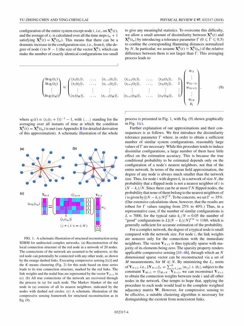
FIG. 1. A schematic illustration of structural reconstruction usingSDBM for undirected complex networks. (a) Reconstruction of thelocal connection structure of the red node in a network of 20 nodes.The connections of the network are assumed to be unknown, so thered node can potentially be connected with any other node, as shownby the orange dashed links. Executing compressive sensing [(c)] andthe K-means clustering (Fig. 2) for this node based on time seriesleads to its true connection structure, marked by the red links. Thelink weights and the nodal bias are represented by the vector VN×1 in(c). (b) All true connections of the network are recovered throughthe process in (a) for each node. The Markov blanket of the rednode in (a) consists of all its nearest neighbors, indicated by thenodes with dashed red circles. (c) A schematic illustration of thecompressive sensing framework for structural reconstruction as inEq. (9).

process is presented in Fig. 1, with Eq. (9) shown graphicallyin Fig. 1(c).

Further explanation of our approximations and their con-sequences is as follows. We first introduce the dissimilaritytolerance parameter � where, in order to obtain a sufficientnumber of similar system configurations, reasonably largevalues of � are necessary. While this procedure tends to inducedissimilar configurations, a large number of them have littleeffect on the estimation accuracy. This is because the trueconditional probability to be estimated depends only on theconfiguration of a node’s nearest neighbors, not that of theentire network. In terms of the mean field approximation, thedegree of any node is always much smaller than the networksize. Thus, for node i with degree ki in a network of size N , theprobability that a flipped node is not a nearest neighbor of i is(N − ki)/N . Since there can be at most �N flipped nodes, theprobability that none of them belong to the nearest neighbors ofi is given by [(N − ki)/N]�N . To be concrete, we set � = 35%.(Our extensive calculations show, however, that the results arerobust for � values ranging from 25% to 40%.) Thus, in arepresentative case, if the number of similar configurations isL = 7000, for the typical ratio ki/N = 0.05 the number of“good” configurations is L[(N − ki)/N ]�N ≈ 1160, which isgenerally sufficient for accurate estimation of the probability.

For a complex network, the degree of a typical node is smallcompared with the network size. For node i, the link weightsare nonzero only for the connections with the immediateneighbors. The vector VN×1 is thus typically sparse with ma-jority of its elements being zero. The sparsity property rendersapplicable compressive sensing [41–46], through which an N

dimensional sparse vector can be reconstructed via a set ofM measurements, for M N . By minimizing the L1 normof VN×1, i.e., ‖VN×1‖1 = ∑N

j=1,j �=i |wij | + |bi |, subject to theconstraint YM×1 = �M×N · VN×1, we can reconstruct VN×1

to obtain the connection weights between node i and all othernodes in the network. One tempts to hope that, applying theprocedure to each node would lead to the complete weightedadjacency matrix W. However, for compressive sensing tobe effective, a suitable clustering algorithm is necessary fordistinguishing the existent from nonexistent links.

032317-4

SPARSE DYNAMICAL BOLTZMANN MACHINE FOR … PHYSICAL REVIEW E 97, 032317 (2018)

2. Necessity of K-means algorithm and implementation

In previous works on reconstruction of complex networksbased on stochastic dynamical correlations [36,37] or com-pressive sensing [27,28], the existent (real) links can be distin-guished from the nonexistent links by setting a single thresholdvalue of certain quantitative measure. The success relies on thefact that the dynamics at various nodes are of the same type,and the reconstruction algorithm is tailored toward the specifictype of dynamical process. Our task is significantly morechallenging as the goal is to develop a system (or a machine)to replicate a diverse array of dynamical processes based ondata for networks with pairwise interactions. For compressivesensing based reconstruction, the computational criteria todistinguish existent from nonexistent links differ substantiallyfor different types of dynamics in terms of quantities such as thesolution magnitude, peak value distribution, and backgroundnoise intensity. As a result, a more elaborate and sophisticatedprocedure is required for determining the threshold for eachparticular case, suggesting that a straightforward applicationof compressive sensing cannot lead to a general reconstructionalgorithm. One may also regard the solutions of the existentlinks as a kind of extreme events [50–52] superimposed ontop of the random background, but it is difficult to devise ageneral criterion to determine if a peak in the distribution ofthe quantitative measure represents the correct extreme eventcorresponding to an actual link.

Through extensive testing, we find that a previously de-veloped unsupervised clustering measure, K means [38,39],possesses the desired traits that can be exploited, in combi-nation with compressive sensing, to develop a reconstructionmachine with pairwise interactions. K means can serve as abase for a highly effective structural estimator for various typesof dynamics on networks of distinct topologies. Dependingon the specific combination of the network topology anddynamics, the reconstruction accuracies vary to certain extentbut are acceptable. Since the compressive sensing operation isnode specific, the solutions obtained separately from differentnodes may give conflicting information as to whether thereis an actual link between the two nodes, requiring a properresolution scheme. We develop such a scheme based on nodedegree consistency. Our reconstruction machine thus containsthree main components: compressive sensing, K means, andconflict resolution. We shall demonstrate in Sec. III that themachine can separate the true positive solutions from the noisybackground with high success rate, for all combinations of thenodal dynamics and the network topology tested.

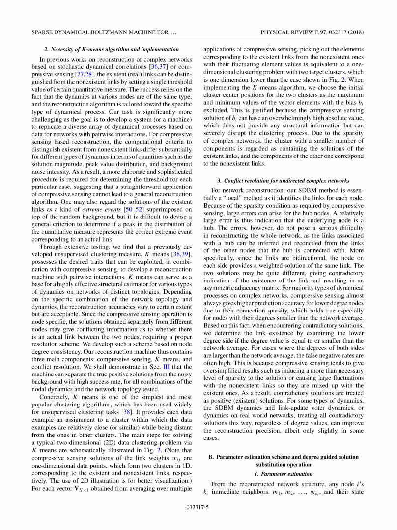
Concretely, K means is one of the simplest and mostpopular clustering algorithms, which has been used widelyfor unsupervised clustering tasks [38]. It provides each dataexample an assignment to a cluster within which the dataexamples are relatively close (or similar) while being distantfrom the ones in other clusters. The main steps for solvinga typical two-dimensional (2D) data clustering problem viaK means are schematically illustrated in Fig. 2. (Note thatcompressive sensing solutions of the link weights wij areone-dimensional data points, which form two clusters in 1D,corresponding to the existent and nonexistent links, respec-tively. The use of 2D illustration is for better visualization.)For each vector VN×1 obtained from averaging over multiple

applications of compressive sensing, picking out the elementscorresponding to the existent links from the nonexistent oneswith their fluctuating element values is equivalent to a one-dimensional clustering problem with two target clusters, whichis one dimension lower than the case shown in Fig. 2. Whenimplementing the K-means algorithm, we choose the initialcluster center positions for the two clusters as the maximumand minimum values of the vector elements with the bias bi

excluded. This is justified because the compressive sensingsolution of bi can have an overwhelmingly high absolute value,which does not provide any structural information but canseverely disrupt the clustering process. Due to the sparsityof complex networks, the cluster with a smaller number ofcomponents is regarded as containing the solutions of theexistent links, and the components of the other one correspondto the nonexistent links.

3. Conflict resolution for undirected complex networks

For network reconstruction, our SDBM method is essen-tially a “local” method as it identifies the links for each node.Because of the sparsity condition as required by compressivesensing, large errors can arise for the hub nodes. A relativelylarge error is thus indication that the underlying node is ahub. The errors, however, do not pose a serious difficultyin reconstructing the whole network, as the links associatedwith a hub can be inferred and reconciled from the linksof the other nodes that the hub is connected with. Morespecifically, since the links are bidirectional, the node oneach side provides a weighted solution of the same link. Thetwo solutions may be quite different, giving contradictoryindication of the existence of the link and resulting in anasymmetric adjacency matrix. For majority types of dynamicalprocesses on complex networks, compressive sensing almostalways gives higher prediction accuracy for lower degree nodesdue to their connection sparsity, which holds true especiallyfor nodes with their degrees smaller than the network average.Based on this fact, when encountering contradictory solutions,we determine the link existence by examining the lowerdegree side if the degree value is equal to or smaller than thenetwork average. For cases where the degrees of both sidesare larger than the network average, the false negative rates areoften high. This is because compressive sensing tends to giveoversimplified results such as inducing a more than necessarylevel of sparsity to the solution or causing large fluctuationswith the nonexistent links so they are mixed up with theexistent ones. As a result, contradictory solutions are treatedas positive (existent) solutions. For some types of dynamics,the SDBM dynamics and link-update voter dynamics, ordynamics on real world networks, treating all contradictorysolutions this way, regardless of degree values, can improvethe reconstruction precision, albeit only slightly in somecases.

B. Parameter estimation scheme and degree guided solutionsubstitution operation

1. Parameter estimation

From the reconstructed network structure, any node i’ski immediate neighbors, m1, m2, . . ., mki

, and their state

032317-5

YU-ZHONG CHEN AND YING-CHENG LAI PHYSICAL REVIEW E 97, 032317 (2018)

FIG. 2. A schematic illustration of the K-means algorithm for two-dimensional data clustering. (a) The data points (solid blue circles) tobe clustered in a 2D feature space. (b) For random locations of the cluster centers (aqua, green, and red hollow circles), each data point can beassociated with the closest center. (c) The 2D space is divided into three regions through three decision boundaries (black dashed lines). (d)Each center moves to the centroid of the data points currently assigned to it (movements shown by the black arrows). (e) The updated clusterassignments of the data points are obtained according to the new center locations. The steps in (c) and (d) are repeated until convergence isachieved. (f) The final cluster assignments.

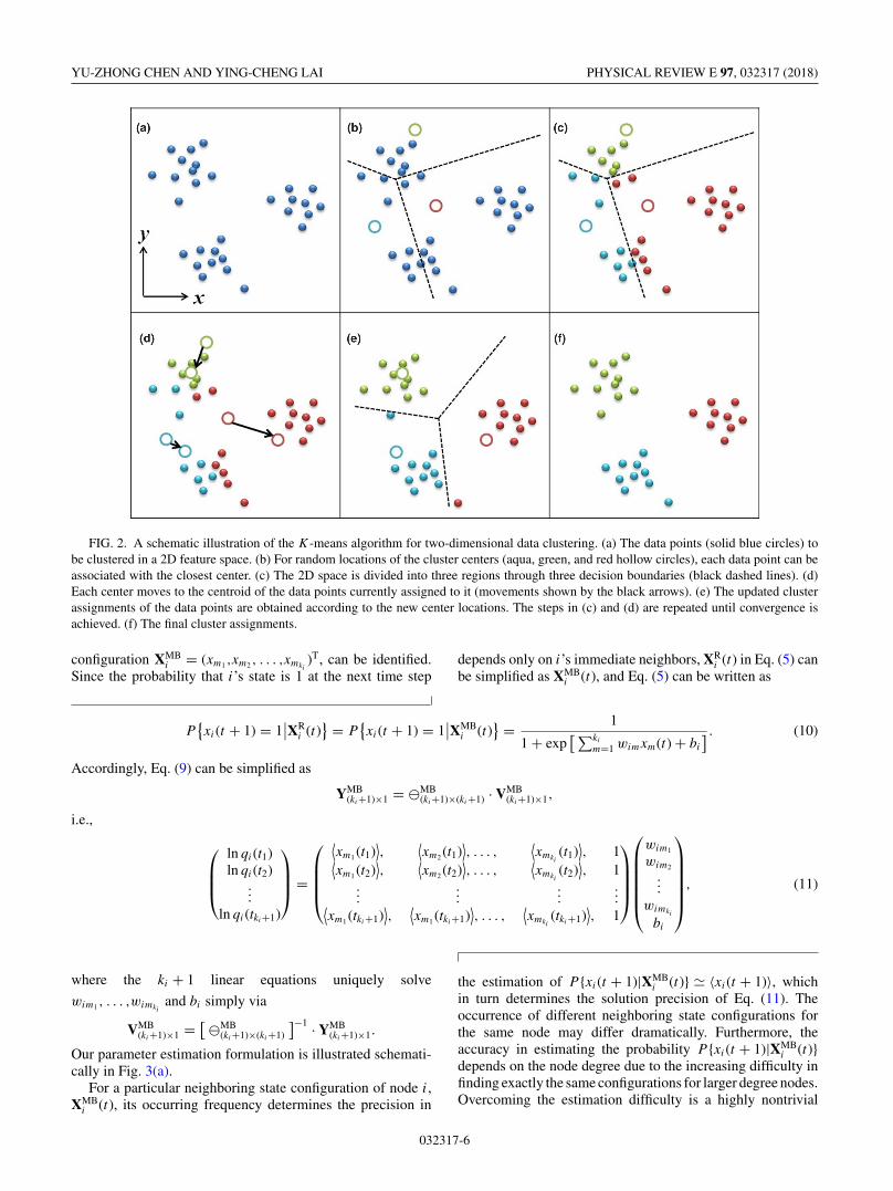
configuration XMBi = (xm1 ,xm2 , . . . ,xmki

)T, can be identified.Since the probability that i’s state is 1 at the next time step

depends only on i’s immediate neighbors, XRi (t) in Eq. (5) can

be simplified as XMBi (t), and Eq. (5) can be written as

P{xi(t + 1) = 1

∣∣XRi (t)

} = P{xi(t + 1) = 1

∣∣XMBi (t)

} = 1

1 + exp[∑ki

m=1 wimxm(t) + bi

] . (10)

Accordingly, Eq. (9) can be simplified as

YMB(ki+1)×1 = �MB

(ki+1)×(ki+1) · VMB(ki+1)×1,

i.e.,

⎛⎜⎜⎝

ln qi(t1)ln qi(t2)

...ln qi(tki+1)

⎞⎟⎟⎠ =

⎛⎜⎜⎜⎝

⟨xm1 (t1)

⟩,

⟨xm2 (t1)

⟩, . . . ,

⟨xmki

(t1)⟩, 1⟨

xm1 (t2)⟩,

⟨xm2 (t2)

⟩, . . . ,

⟨xmki

(t2)⟩, 1

......

......⟨

xm1 (tki+1)⟩,

⟨xm1 (tki+1)

⟩, . . . ,

⟨xmki

(tki+1)⟩, 1

⎞⎟⎟⎟⎠

⎛⎜⎜⎜⎜⎜⎝

wim1

wim2

...wimki

bi

⎞⎟⎟⎟⎟⎟⎠, (11)

where the ki + 1 linear equations uniquely solve

wim1 , . . . ,wimkiand bi simply via

VMB(ki+1)×1 = [ �MB

(ki+1)×(ki+1)

]−1 · YMB(ki+1)×1.

Our parameter estimation formulation is illustrated schemati-cally in Fig. 3(a).

For a particular neighboring state configuration of node i,XMB

i (t), its occurring frequency determines the precision in

the estimation of P {xi(t + 1)|XMBi (t)} � 〈xi(t + 1)〉, which

in turn determines the solution precision of Eq. (11). Theoccurrence of different neighboring state configurations forthe same node may differ dramatically. Furthermore, theaccuracy in estimating the probability P {xi(t + 1)|XMB

i (t)}depends on the node degree due to the increasing difficulty infinding exactly the same configurations for larger degree nodes.Overcoming the estimation difficulty is a highly nontrivial

032317-6

SPARSE DYNAMICAL BOLTZMANN MACHINE FOR … PHYSICAL REVIEW E 97, 032317 (2018)

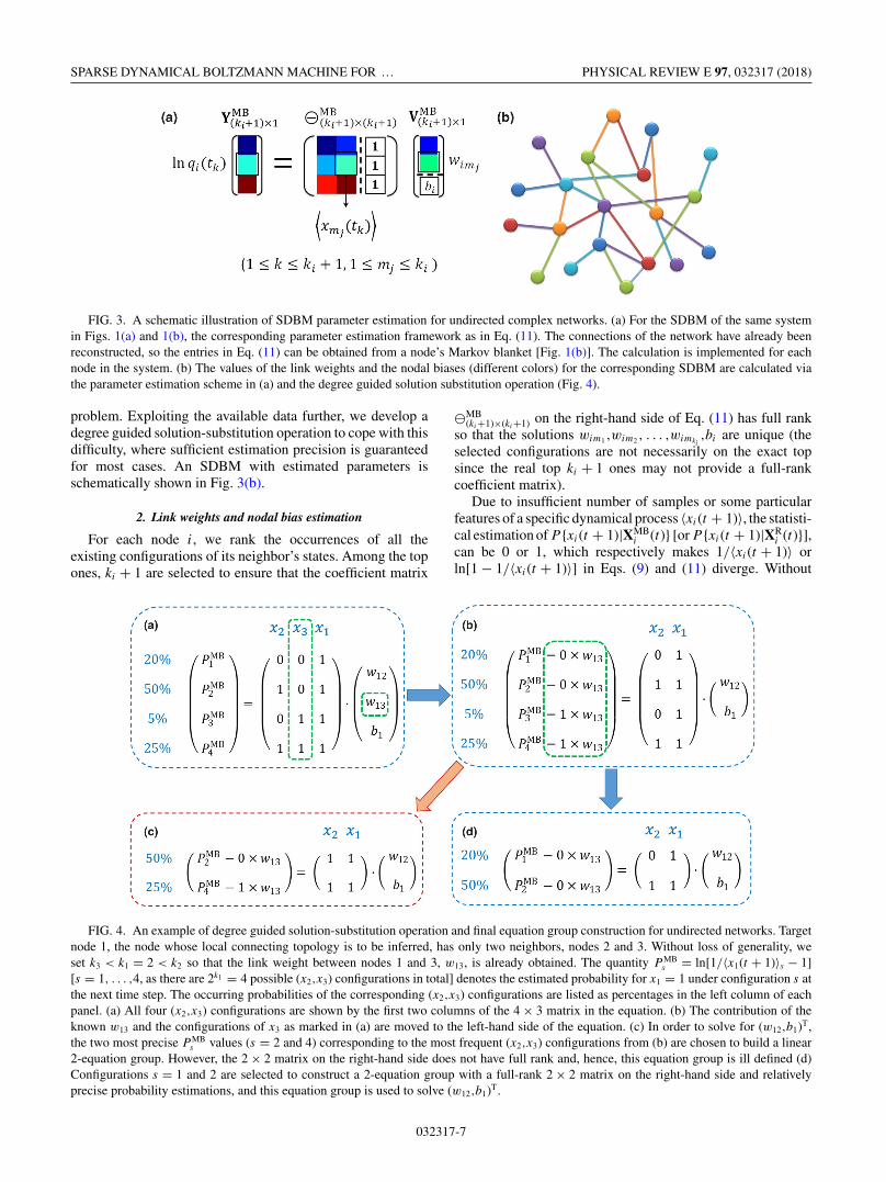
FIG. 3. A schematic illustration of SDBM parameter estimation for undirected complex networks. (a) For the SDBM of the same systemin Figs. 1(a) and 1(b), the corresponding parameter estimation framework as in Eq. (11). The connections of the network have already beenreconstructed, so the entries in Eq. (11) can be obtained from a node’s Markov blanket [Fig. 1(b)]. The calculation is implemented for eachnode in the system. (b) The values of the link weights and the nodal biases (different colors) for the corresponding SDBM are calculated viathe parameter estimation scheme in (a) and the degree guided solution substitution operation (Fig. 4).

problem. Exploiting the available data further, we develop adegree guided solution-substitution operation to cope with thisdifficulty, where sufficient estimation precision is guaranteedfor most cases. An SDBM with estimated parameters isschematically shown in Fig. 3(b).

2. Link weights and nodal bias estimation

For each node i, we rank the occurrences of all theexisting configurations of its neighbor’s states. Among the topones, ki + 1 are selected to ensure that the coefficient matrix

�MB(ki+1)×(ki+1) on the right-hand side of Eq. (11) has full rank

so that the solutions wim1 ,wim2 , . . . ,wimki,bi are unique (the

selected configurations are not necessarily on the exact topsince the real top ki + 1 ones may not provide a full-rankcoefficient matrix).

Due to insufficient number of samples or some particularfeatures of a specific dynamical process 〈xi(t + 1)〉, the statisti-cal estimation of P {xi(t + 1)|XMB

i (t)} [or P {xi(t + 1)|XRi (t)}],

can be 0 or 1, which respectively makes 1/〈xi(t + 1)〉 orln[1 − 1/〈xi(t + 1)〉] in Eqs. (9) and (11) diverge. Without

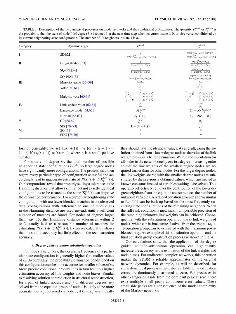
FIG. 4. An example of degree guided solution-substitution operation and final equation group construction for undirected networks. Targetnode 1, the node whose local connecting topology is to be inferred, has only two neighbors, nodes 2 and 3. Without loss of generality, weset k3 < k1 = 2 < k2 so that the link weight between nodes 1 and 3, w13, is already obtained. The quantity P MB

s = ln[1/〈x1(t + 1)〉s − 1][s = 1, . . . ,4, as there are 2k1 = 4 possible (x2,x3) configurations in total] denotes the estimated probability for x1 = 1 under configuration s atthe next time step. The occurring probabilities of the corresponding (x2,x3) configurations are listed as percentages in the left column of eachpanel. (a) All four (x2,x3) configurations are shown by the first two columns of the 4 × 3 matrix in the equation. (b) The contribution of theknown w13 and the configurations of x3 as marked in (a) are moved to the left-hand side of the equation. (c) In order to solve for (w12,b1)T,the two most precise P MB

s values (s = 2 and 4) corresponding to the most frequent (x2,x3) configurations from (b) are chosen to build a linear2-equation group. However, the 2 × 2 matrix on the right-hand side does not have full rank and, hence, this equation group is ill defined (d)Configurations s = 1 and 2 are selected to construct a 2-equation group with a full-rank 2 × 2 matrix on the right-hand side and relativelyprecise probability estimations, and this equation group is used to solve (w12,b1)T.

032317-7

YU-ZHONG CHEN AND YING-CHENG LAI PHYSICAL REVIEW E 97, 032317 (2018)

TABLE I. Description of the 14 dynamical processes on model networks and the conditional probabilities. The quantity P 0→1i or P 1→0

i isthe probability that the state of node i (of degree ki) becomes 1 at the next time step when its current state is 0, or vice versa, conditioned onits current neighboring state configuration. The number of i’s neighbors in state 1 is ni .

Category Dynamics type P 0→1i P 1→0

i

I SDBM 11+exp[

∑Nj=1,j �=i wij xj (t)+bi ]

exp[∑N

j=1,j �=i wij xj (t)+bi ]

1+exp[∑N

j=1,j �=i wij xj (t)+bi ]

II Ising-Glauber [53] 11+exp[ 2J

κ (ki−2ni )]

exp[ 2Jκ (ki−2ni )]

1+exp[ 2Jκ (ki−2ni )]

SQ-SG [54] 11+exp[(rki−ni )/κ]

exp[(rki−ni )/κ]1+exp[(rki−ni )/κ]

SQ-PDG [54] 11+exp[(b−1)(ki−ni )/κ]

exp[(b−1)(ki−ni )/κ]1+exp[(b−1)(ki−ni )/κ]

III Minority game [55–59] ki−ni

ki

ni

ki

Voter [60,61] ni

ki

ki−ni

ki

Majority vote [60,61]

{Q if ni < ki/21/2 if ni = ki/21 − Q if ni > ki/2

{1 − Q if ni < ki/21/2 if ni = ki/2Q if ni > ki/2

IV Link-update voter [62,63] ni

〈k〉ki−ni

〈k〉Language model[64,65] S( ni

ki)α (1 − S)( ki−ni

ki)α

Kirman [66,67] c1 + dni c2 + d(ki − ni)

V CP [68,69] ni

kiλi μi

SIS [70–73] 1 − (1 − λi)ni μi

VI SG [74] * *PDG [75,76] * *

loss of generality, we set 〈xi(t + 1)〉 = ε [or 〈xi(t + 1)〉 =1 − ε] if 〈xi(t + 1)〉 = 0 (or 1), where ε is a small positiveconstant.

For node i of degree ki , the total number of possibleneighboring state configurations is 2ki , so large degree nodeshave significantly more configurations. The process may thenregard every particular type of configuration as useful and ac-cordingly lead to inaccurate estimate of P {xi(t + 1)|XMB

i (t)}.Our computations reveal that properly setting a tolerance in theHamming distance that allows similar but not exactly identicalconfigurations to be treated as the same XMB

i (t) can improvethe estimation performance. For a particular neighboring stateconfiguration with too fewer identical matches in the observeddata, configurations with difference in one or more digitsin the Hamming distance are used instead, until a sufficientnumber of matches are found. For nodes of degrees largerthan, say 15, the Hamming distance tolerances within 2or 3 usually lead to a reasonable number of matches forestimating P {xi(t + 1)|XMB

i (t)}. Extensive calculation showsthat the small inaccuracy has little effect on the reconstructionaccuracy.

3. Degree guided solution substitution operation

For node i’s neighbors, the occurring frequency of a partic-ular state configuration is generally higher for smaller valuesof ki . Accordingly, the probability estimation conditioned onthis configuration can be more accurate for smaller values of ki .More precise conditional probabilities in turn lead to a higherestimation accuracy of link weights and node biases. Similarto resolving solution contradiction in structural reconstruction,for a pair of linked nodes, i and j of different degrees, wij

solved from the equation group of node i is likely to be moreaccurate than wji obtained via node j , if ki < kj , even ideally

they should have the identical values. As a result, using the so-lution obtained from a lower degree node as the value of the linkweight provides a better estimation. We run the calculation forall nodes in the network one by one in a degree-increasing orderso that the link weights of the smallest degree nodes are ac-quired earlier than for other nodes. For the larger degree nodes,the link weights shared with the smaller degree nodes are sub-stituted by the previously obtained values, which are treated asknown constants instead of variables waiting to be solved. Thisoperation effectively removes the contribution of the lower de-gree neighbors from the equation and so reduces the number ofunknown variables. A reduced equation group in a form similarto Eq. (11) can be built up based on the most frequently oc-curring state configurations of the remaining neighbors. Whenthe full-rank condition is met, maximum possible precision ofthe remaining unknown link weights can be achieved. Conse-quently, with the substitution operation, the ki link weights ofnode i, which can be inaccurate if solved from the original (ki +1)-equation group, can be estimated with the maximum possi-ble accuracy. An example of this substitution operation and thefinal equation group construction process is shown in Fig. 4.

Our calculations show that the application of the degreeguided solution-substitution operation can significantlyincrease the accuracy in the estimation of the link weights andnode biases. For undirected complex networks, this operationmakes the SDBM a reliable approximator of the originalnetwork dynamics. For example, as will be described, forsome dynamical processes described in Table I, the estimationerrors are dominantly distributed at zero. For processes inother categories, aside from the dominant peak at zero, thereexist multiple small peaks at nonzero error values. Thesesmall side peaks are a consequence of the model complexityof the Markov networks.

032317-8

SPARSE DYNAMICAL BOLTZMANN MACHINE FOR … PHYSICAL REVIEW E 97, 032317 (2018)

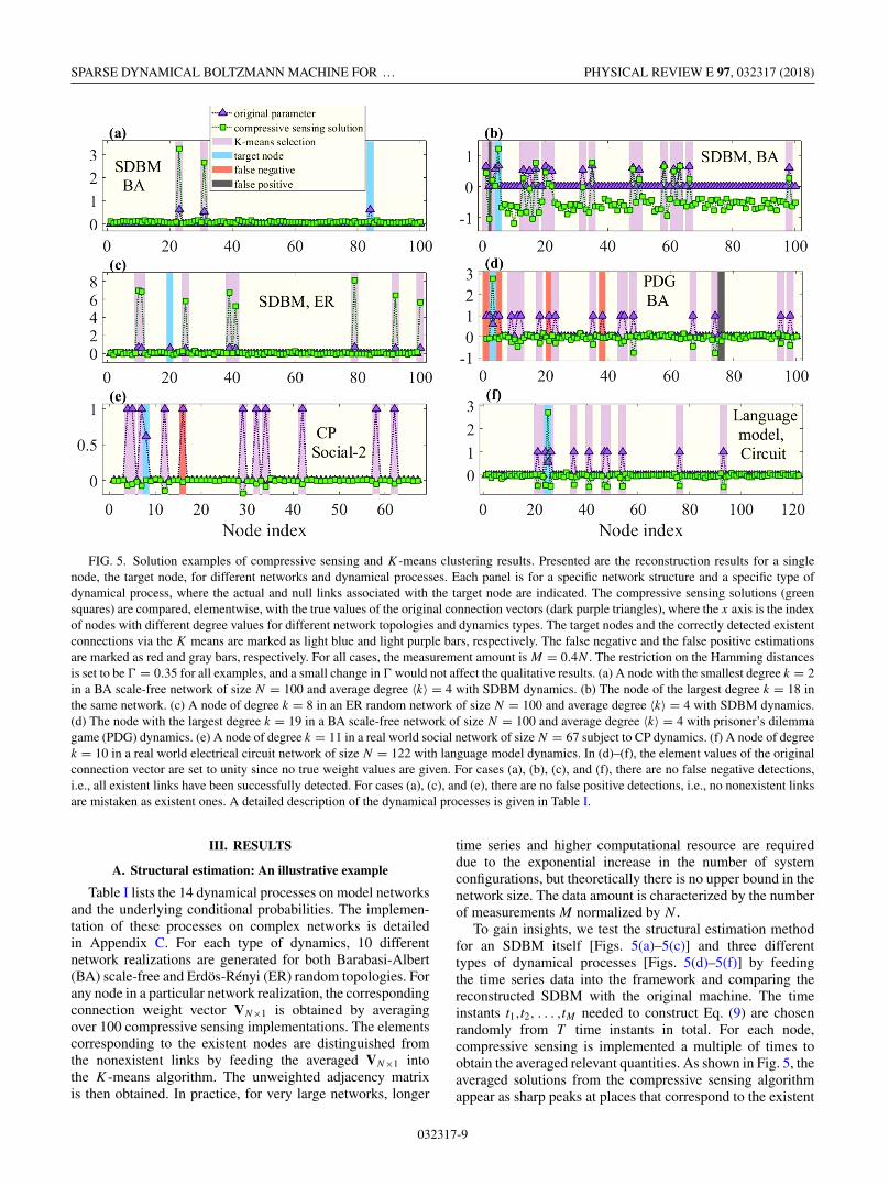
FIG. 5. Solution examples of compressive sensing and K-means clustering results. Presented are the reconstruction results for a singlenode, the target node, for different networks and dynamical processes. Each panel is for a specific network structure and a specific type ofdynamical process, where the actual and null links associated with the target node are indicated. The compressive sensing solutions (greensquares) are compared, elementwise, with the true values of the original connection vectors (dark purple triangles), where the x axis is the indexof nodes with different degree values for different network topologies and dynamics types. The target nodes and the correctly detected existentconnections via the K means are marked as light blue and light purple bars, respectively. The false negative and the false positive estimationsare marked as red and gray bars, respectively. For all cases, the measurement amount is M = 0.4N . The restriction on the Hamming distancesis set to be � = 0.35 for all examples, and a small change in � would not affect the qualitative results. (a) A node with the smallest degree k = 2in a BA scale-free network of size N = 100 and average degree 〈k〉 = 4 with SDBM dynamics. (b) The node of the largest degree k = 18 inthe same network. (c) A node of degree k = 8 in an ER random network of size N = 100 and average degree 〈k〉 = 4 with SDBM dynamics.(d) The node with the largest degree k = 19 in a BA scale-free network of size N = 100 and average degree 〈k〉 = 4 with prisoner’s dilemmagame (PDG) dynamics. (e) A node of degree k = 11 in a real world social network of size N = 67 subject to CP dynamics. (f) A node of degreek = 10 in a real world electrical circuit network of size N = 122 with language model dynamics. In (d)–(f), the element values of the originalconnection vector are set to unity since no true weight values are given. For cases (a), (b), (c), and (f), there are no false negative detections,i.e., all existent links have been successfully detected. For cases (a), (c), and (e), there are no false positive detections, i.e., no nonexistent linksare mistaken as existent ones. A detailed description of the dynamical processes is given in Table I.

III. RESULTS

A. Structural estimation: An illustrative example

Table I lists the 14 dynamical processes on model networksand the underlying conditional probabilities. The implemen-tation of these processes on complex networks is detailedin Appendix C. For each type of dynamics, 10 differentnetwork realizations are generated for both Barabasi-Albert(BA) scale-free and Erdös-Rényi (ER) random topologies. Forany node in a particular network realization, the correspondingconnection weight vector VN×1 is obtained by averagingover 100 compressive sensing implementations. The elementscorresponding to the existent nodes are distinguished fromthe nonexistent links by feeding the averaged VN×1 intothe K-means algorithm. The unweighted adjacency matrixis then obtained. In practice, for very large networks, longer

time series and higher computational resource are requireddue to the exponential increase in the number of systemconfigurations, but theoretically there is no upper bound in thenetwork size. The data amount is characterized by the numberof measurements M normalized by N .

To gain insights, we test the structural estimation methodfor an SDBM itself [Figs. 5(a)–5(c)] and three differenttypes of dynamical processes [Figs. 5(d)–5(f)] by feedingthe time series data into the framework and comparing thereconstructed SDBM with the original machine. The timeinstants t1,t2, . . . ,tM needed to construct Eq. (9) are chosenrandomly from T time instants in total. For each node,compressive sensing is implemented a multiple of times toobtain the averaged relevant quantities. As shown in Fig. 5, theaveraged solutions from the compressive sensing algorithmappear as sharp peaks at places that correspond to the existent

032317-9

YU-ZHONG CHEN AND YING-CHENG LAI PHYSICAL REVIEW E 97, 032317 (2018)

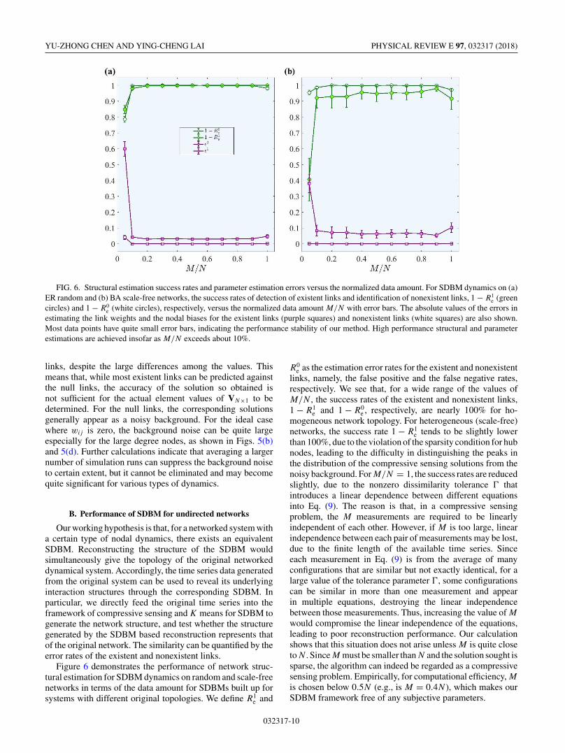
FIG. 6. Structural estimation success rates and parameter estimation errors versus the normalized data amount. For SDBM dynamics on (a)ER random and (b) BA scale-free networks, the success rates of detection of existent links and identification of nonexistent links, 1 − R1

e (greencircles) and 1 − R0

e (white circles), respectively, versus the normalized data amount M/N with error bars. The absolute values of the errors inestimating the link weights and the nodal biases for the existent links (purple squares) and nonexistent links (white squares) are also shown.Most data points have quite small error bars, indicating the performance stability of our method. High performance structural and parameterestimations are achieved insofar as M/N exceeds about 10%.

links, despite the large differences among the values. Thismeans that, while most existent links can be predicted againstthe null links, the accuracy of the solution so obtained isnot sufficient for the actual element values of VN×1 to bedetermined. For the null links, the corresponding solutionsgenerally appear as a noisy background. For the ideal casewhere wij is zero, the background noise can be quite largeespecially for the large degree nodes, as shown in Figs. 5(b)and 5(d). Further calculations indicate that averaging a largernumber of simulation runs can suppress the background noiseto certain extent, but it cannot be eliminated and may becomequite significant for various types of dynamics.

B. Performance of SDBM for undirected networks

Our working hypothesis is that, for a networked system witha certain type of nodal dynamics, there exists an equivalentSDBM. Reconstructing the structure of the SDBM wouldsimultaneously give the topology of the original networkeddynamical system. Accordingly, the time series data generatedfrom the original system can be used to reveal its underlyinginteraction structures through the corresponding SDBM. Inparticular, we directly feed the original time series into theframework of compressive sensing and K means for SDBM togenerate the network structure, and test whether the structuregenerated by the SDBM based reconstruction represents thatof the original network. The similarity can be quantified by theerror rates of the existent and nonexistent links.

Figure 6 demonstrates the performance of network struc-tural estimation for SDBM dynamics on random and scale-freenetworks in terms of the data amount for SDBMs built up forsystems with different original topologies. We define R1

e and

R0e as the estimation error rates for the existent and nonexistent

links, namely, the false positive and the false negative rates,respectively. We see that, for a wide range of the values ofM/N , the success rates of the existent and nonexistent links,1 − R1

e and 1 − R0e , respectively, are nearly 100% for ho-

mogeneous network topology. For heterogeneous (scale-free)networks, the success rate 1 − R1

e tends to be slightly lowerthan 100%, due to the violation of the sparsity condition for hubnodes, leading to the difficulty in distinguishing the peaks inthe distribution of the compressive sensing solutions from thenoisy background. For M/N = 1, the success rates are reducedslightly, due to the nonzero dissimilarity tolerance � thatintroduces a linear dependence between different equationsinto Eq. (9). The reason is that, in a compressive sensingproblem, the M measurements are required to be linearlyindependent of each other. However, if M is too large, linearindependence between each pair of measurements may be lost,due to the finite length of the available time series. Sinceeach measurement in Eq. (9) is from the average of manyconfigurations that are similar but not exactly identical, for alarge value of the tolerance parameter �, some configurationscan be similar in more than one measurement and appearin multiple equations, destroying the linear independencebetween those measurements. Thus, increasing the value of M

would compromise the linear independence of the equations,leading to poor reconstruction performance. Our calculationshows that this situation does not arise unless M is quite closetoN . SinceM must be smaller thanN and the solution sought issparse, the algorithm can indeed be regarded as a compressivesensing problem. Empirically, for computational efficiency, Mis chosen below 0.5N (e.g., is M = 0.4N ), which makes ourSDBM framework free of any subjective parameters.

032317-10

SPARSE DYNAMICAL BOLTZMANN MACHINE FOR … PHYSICAL REVIEW E 97, 032317 (2018)

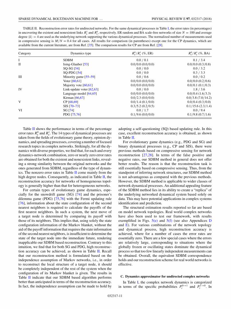
TABLE II. Reconstruction error rates for undirected networks. For the same dynamical processes in Table I, the error rates (in percentages)in uncovering the existent and nonexistent links R1

e and R0e , respectively. ER random and BA scale-free networks of size N = 100 and average

degree 〈k〉 = 4 are used as the underlying network supporting the various dynamical processes. The normalized number of measurements usedin compressive sensing is M/N = 0.4 for all cases. All results for comparison (in parentheses) except one for the CP dynamics, which areavailable from the current literature, are from Ref. [35]. The comparison results for CP are from Ref. [28].

Category Dynamics type R0e /R

1e (%, ER) R0

e /R1e (%, BA)

I SDBM 0.0 / 0.1 0.1 / 3.4II Ising-Glauber [53] 0.0/0.0 (0.0/0.0) 0.0/0.0 (0.3/0.8)

SQ-SG [54] 0.0 / 0.0 0.0 / 3.2SQ-PDG [54] 0.0 / 0.0 0.3 / 3.3

III Minority game [55–59] 0.0 / 0.6 0.0 / 0.2Voter [60,61] 0.0/0.0 (0.0/0.0) 0.0/0.0 (0.2/0.6)Majority vote [60,61] 0.0/0.0 (0.0/0.0) 0.0/0.1 (0.1/0.3)

IV Link-update voter [62,63] 0.0 / 0.0 1.8 / 3.6Language model [64,65] 0.0/0.0 (0.0/0.0) 0.0/0.4 (1.6/3.3)Kirman [66,67] 0.0/2.3 (0.0/0.0) 0.0/3.8 (7.0/14.2)

V CP [68,69] 0.0/1.4 (0.1/0.0) 0.0/0.4 (0.3/0.0)SIS [70–73] 0.3/5.2 (0.2/0.5) 0.1/15.6 (2.3/1.4)

VI SG [74] 0.0 / 1.7 0.0 / 9.4PDG [75,76] 0.1/9.6 (0.0/0.0) 0.1/9.8 (0.7/1.6)

Table II shows the performance in terms of the percentageerror rates R0

e and R1e . The 14 types of dynamical processes are

taken from the fields of evolutionary game theory, opinion dy-namics, and spreading processes, covering a number of focusedresearch topics in complex networks. Strikingly, for all the dy-namics with diverse properties, we find that, for each and everydynamics-network combination, zero or nearly zero error ratesare obtained for both the existent and nonexistent links, reveal-ing a strong similarity between the original networks and theones generated from SDBM, regardless of the type of dynam-ics. The nonzero error rates in Table II come mainly from thehigh degree nodes. Consequently, as indicated in Table II, thereconstruction accuracy for networks of homogeneous topol-ogy is generally higher than that for heterogeneous networks.

For certain types of evolutionary game dynamics, espe-cially for the snowdrift game (SG) [74] and the prisoner’sdilemma game (PDG) [75,76] with the Fermi updating rule[76], information about the state configuration of the secondnearest neighbors is required to calculate the payoffs of thefirst nearest neighbors. In such a system, the next move ofa target node is determined by comparing its payoff withthose of its neighbors. This implies that, using solely the stateconfiguration information of the Markov blanket, without theaid of the payoff information that requires the state informationof the second nearest neighbors, is insufficient to determine thestate of the target node into the immediate future, renderinginapplicable our SDBM based reconstruction. Contrary to thisintuition, we find that for both SG and PDG, high reconstruc-tion accuracy can be achieved, as shown in Table II. Recallthat our reconstruction method is formulated based on theindependence assumption of Markov networks, i.e., in orderto reconstruct the local structure of a target node, it shouldbe completely independent of the rest of the system when theconfiguration of its Markov blanket is given. The results inTable II indicate that our SDBM based algorithm performsbetter than anticipated in terms of the reconstruction accuracy.In fact, the independence assumption can be made to hold by

adopting a self-questioning (SQ) based updating rule. In thiscase, excellent reconstruction accuracy is obtained, as shownin Table II.

For evolutionary game dynamics (e.g., PDG and SG) andbinary dynamical processes (e.g., CP and SIS), there wereprevious methods based on compressive sensing for networkreconstruction [27,28]. In terms of the false positive andnegative rates, our SDBM method in general does not offerbetter results. The reason is that the reconstruction task isstill essentially based on compressive sensing. Thus, from thestandpoint of inferring network structures, our SDBM methodis not advantageous as compared with the previous methods.However, the SDBM method is applicable to wider classes ofnetwork dynamical processes. An additional appealing featureof the SDBM method lies in its ability to create a “replica” ofthe underlying networked dynamical system based solely ondata. This may have potential applications in complex systemsidentification and prediction.

The structural estimation results reported so far are basedon model network topologies. Real world complex networkshave also been used to test our framework, with resultsexemplified in Figs. 5(e) and 5(f) (see also Appendices Dand E). For various combinations of the network topologyand dynamical process, high reconstruction accuracy isachieved, where for a number of cases the error rates areessentially zero. There are a few special cases where the errorsare relatively large, corresponding to situations where theglobally frozen or oscillating states dominate the dynamicalprocess so that too few linearly independent measurements canbe obtained. Overall, the equivalent SDBM correspondenceholds and our reconstruction scheme for real world networks iseffective.

C. Dynamics approximator for undirected complex networks

In Table I, the complex network dynamics is categorizedin terms of the specific probabilities P 0→1

i and P 1→0i . In

032317-11

YU-ZHONG CHEN AND YING-CHENG LAI PHYSICAL REVIEW E 97, 032317 (2018)

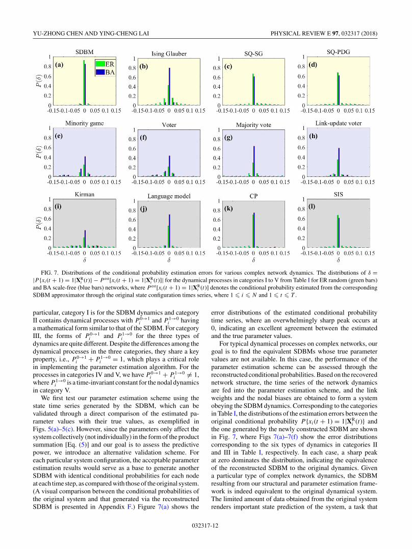
FIG. 7. Distributions of the conditional probability estimation errors for various complex network dynamics. The distributions of δ =|P {xi(t + 1) = 1|XR

i (t)} − P est[xi(t + 1) = 1|XRi (t)]| for the dynamical processes in categories I to V from Table I for ER random (green bars)

and BA scale-free (blue bars) networks, where P est[xi(t + 1) = 1|XRi (t)] denotes the conditional probability estimated from the corresponding

SDBM approximator through the original state configuration times series, where 1 � i � N and 1 � t � T .

particular, category I is for the SDBM dynamics and categoryII contains dynamical processes with P 0→1

i and P 1→0i having

a mathematical form similar to that of the SDBM. For categoryIII, the forms of P 0→1

i and P 1→0i for the three types of

dynamics are quite different. Despite the differences among thedynamical processes in the three categories, they share a keyproperty, i.e., P 0→1

i + P 1→0i = 1, which plays a critical role

in implementing the parameter estimation algorithm. For theprocesses in categories IV and V, we have P 0→1

i + P 1→0i �= 1,

where P 1→0i is a time-invariant constant for the nodal dynamics

in category V.We first test our parameter estimation scheme using the

state time series generated by the SDBM, which can bevalidated through a direct comparison of the estimated pa-rameter values with their true values, as exemplified inFigs. 5(a)–5(c). However, since the parameters only affect thesystem collectively (not individually) in the form of the productsummation [Eq. (5)] and our goal is to assess the predictivepower, we introduce an alternative validation scheme. Foreach particular system configuration, the acceptable parameterestimation results would serve as a base to generate anotherSDBM with identical conditional probabilities for each nodeat each time step, as compared with those of the original system.(A visual comparison between the conditional probabilities ofthe original system and that generated via the reconstructedSDBM is presented in Appendix F.) Figure 7(a) shows the

error distributions of the estimated conditional probabilitytime series, where an overwhelmingly sharp peak occurs at0, indicating an excellent agreement between the estimatedand the true parameter values.

For typical dynamical processes on complex networks, ourgoal is to find the equivalent SDBMs whose true parametervalues are not available. In this case, the performance of theparameter estimation scheme can be assessed through thereconstructed conditional probabilities. Based on the recoverednetwork structure, the time series of the network dynamicsare fed into the parameter estimation scheme, and the linkweights and the nodal biases are obtained to form a systemobeying the SDBM dynamics. Corresponding to the categoriesin Table I, the distributions of the estimation errors between theoriginal conditional probability P {xi(t + 1) = 1|XR

i (t)} andthe one generated by the newly constructed SDBM are shownin Fig. 7, where Figs 7(a)–7(f) show the error distributionscorresponding to the six types of dynamics in categories IIand III in Table I, respectively. In each case, a sharp peakat zero dominates the distribution, indicating the equivalenceof the reconstructed SDBM to the original dynamics. Givena particular type of complex network dynamics, the SDBMresulting from our structural and parameter estimation frame-work is indeed equivalent to the original dynamical system.The limited amount of data obtained from the original systemrenders important state prediction of the system, a task that

032317-12

SPARSE DYNAMICAL BOLTZMANN MACHINE FOR … PHYSICAL REVIEW E 97, 032317 (2018)

can be accomplished by taking advantage of the equivalenceof the SDBM to the original system in the sense that the SDBMproduces approximately equal state transition probabilitiesin the immediate future, given the current system config-uration. The SDBM thus possesses a significant predictivepower for the original system. Regardless of the type of thedynamical process, insofar it satisfies the relation P 0→1

i +P 1→0

i = 1, the reconstructed SDBM can serve as a dynamicsapproximator.

For an SDBM, the relation P 1→1i = 1 − P 1→0

i = P 0→1i

holds in general. However, for the dynamical processes incategories IV and V, we have P 1→1

i �= 1 − P 1→0i = P 0→1

i

so that a single SDBM is not sufficient to fully characterizethe dynamical evolution. Our solution is to construct twoSDBMs, A and B, each associated with one of the two cases:xi(t) = 0 and xi(t) = 1, respectively. The link weights wA

ij

(or wBij ) and the nodal bias bA

i (or bBi ) for node i in SDBM

A (or B) are computed for all the time steps t satisfyingxi(t) = 0 [or xi(t) = 1], leading to P {xi(t + 1) = 1|XR

i (t)}for xi(t) = 0 [or xi(t) = 1] from SDBM A (or B). Usingthis strategy, the dominant peaks at zero persist in the errordistributions for the dynamical processes in category IV, asshown in Figs. 7(g)–7(j). For the epidemic spreading dynamics(CP and SIS) in category V, the fixed value of P 1→0

i foreach node i can be acquired through P 1→0

i � 〈xi(t1 + 1)〉t1 ,where 〈xi(t1 + 1)〉t1 stands for the average of xi(t1 + 1) overall values of t1 satisfying xi(t1) = 1. Through this approach,SDBM B is in fact a network without links but with eachnode’s bias satisfying μi = exp(bi)/[1 + exp(bi)], where μi

is node i’s recovery rate. Figures 7(k) and 7(l) show theerror distributions of the conditional probability recovery forthe spreading processes, where we see that the errors areessentially zero. If the method of solving SDBM B in categoryIV is adopted to the dynamical processes in other categories,i.e., without any prior knowledge about P 1→0

i , the resultedSDBM would have nearly identical link weight values withrespect to SDBM A (in categories I–III) or have close-to-zerolink weights and μi � exp(bi)/[1 + exp(bi)] for category V,despite that their conditional probability recovery errors maybe slightly larger than those in Fig. 7. The persistent occurrenceof a dominant peak at zero in the error distribution suggeststhe power of combined SDBMs as a dynamics approximator,regardless of the specifics of the transition probability. Whenlimited prior knowledge about P 1→0

i is available, SDBM Bcan be simplified or even removed without compromisingthe estimation accuracy. In general, the approximator has asignificant short-term predictive power for arbitrary types ofdynamics on complex networks.

The conditional probability recovery error is called the“training error” since it is obtained from the same data setused to build (or “train”) the approximator, and the datapoints generated from the same system that have not beenused in the training process can be exploited to validate ortest the actual performance of the trained model [38], whichin our case is the approximator. As a result, the time seriesgenerated from the original complex network system afterthe approximator is built can be used as the test data set.(Absence of hyperparameters in the reconstruction processmeans that cross validation is unnecessary.) In most cases,

the training errors are generally smaller than the test errorssince the training data set is already well fitted by the model(the approximator) in the training process, while the test dataare new and may be out of the fitting range of the currentmodel. Feeding the state configurations of the test data set intothe approximator, we calculate the corresponding conditionalprobabilities using Eq. (5) and compare them to the truevalues. The results reveal a clear advantage of the approximatorbuilt from our scheme, i.e., the training and test errors arenearly identical, indicating the absence of any overfittingissues [38].

D. Extension to directed complex networks

Our SDBM methodology for undirected networks can beadapted to directed networks because of its nodewise imple-mentation scheme. In a directed network, the link weightsbetween nodes i and j , wij and wji , do not have equal values. Infact, these are weights of the two links in the opposite directionsbetween the same pair of nodes. The weights solved by Eqs. (9)and (11) correspond to all the links pointing to node i and allpointing from i’s nearest neighbors. By estimating the values ofthe inward link weights for each node in the network, we obtaina directed SDBM as a structural estimator and dynamics ap-proximator of the underlying directed network. The structuraland parameter estimation processes are illustrated in Figs. 8(a)and 8(b). Since the conflict resolution scheme designed forundirected networks applies to symmetric links only, it is notadopted for directed networks. The structural estimation resultsare presented in Table III. In most cases, we observe only smallchanges in the precision as compared with the undirected case.For some types of dynamics, R0

e increases slightly, indicatingthat the main challenge of reconstructing directed networksis to reduce the false positives. Nonetheless, in general, the

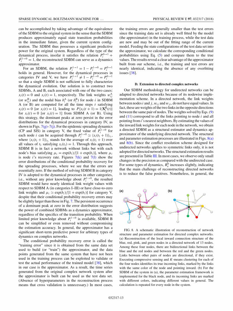
FIG. 8. A schematic illustration of reconstruction of networkstructure and parameter estimation for directed complex networks.(a) Reconstruction of the local inward connection structure of theblue, red, pink, and green nodes in a directed network of 13 nodes.Among these four nodes, there are bidirectional links between theblue and the red nodes and between the red and the green nodes.Links between other pairs of nodes are directional, if they exist.Executing compressive sensing and K-means clustering for each ofthe four nodes identifies its true incoming links, marked by the linkswith the same color of the node and pointing inward. (b) For theSDBM of the system in (a), the parameter estimation framework isimplemented for the black node, and its incoming links are markedwith different colors, indicating different values in general. Thecalculation is repeated for every node in the system.

032317-13

YU-ZHONG CHEN AND YING-CHENG LAI PHYSICAL REVIEW E 97, 032317 (2018)

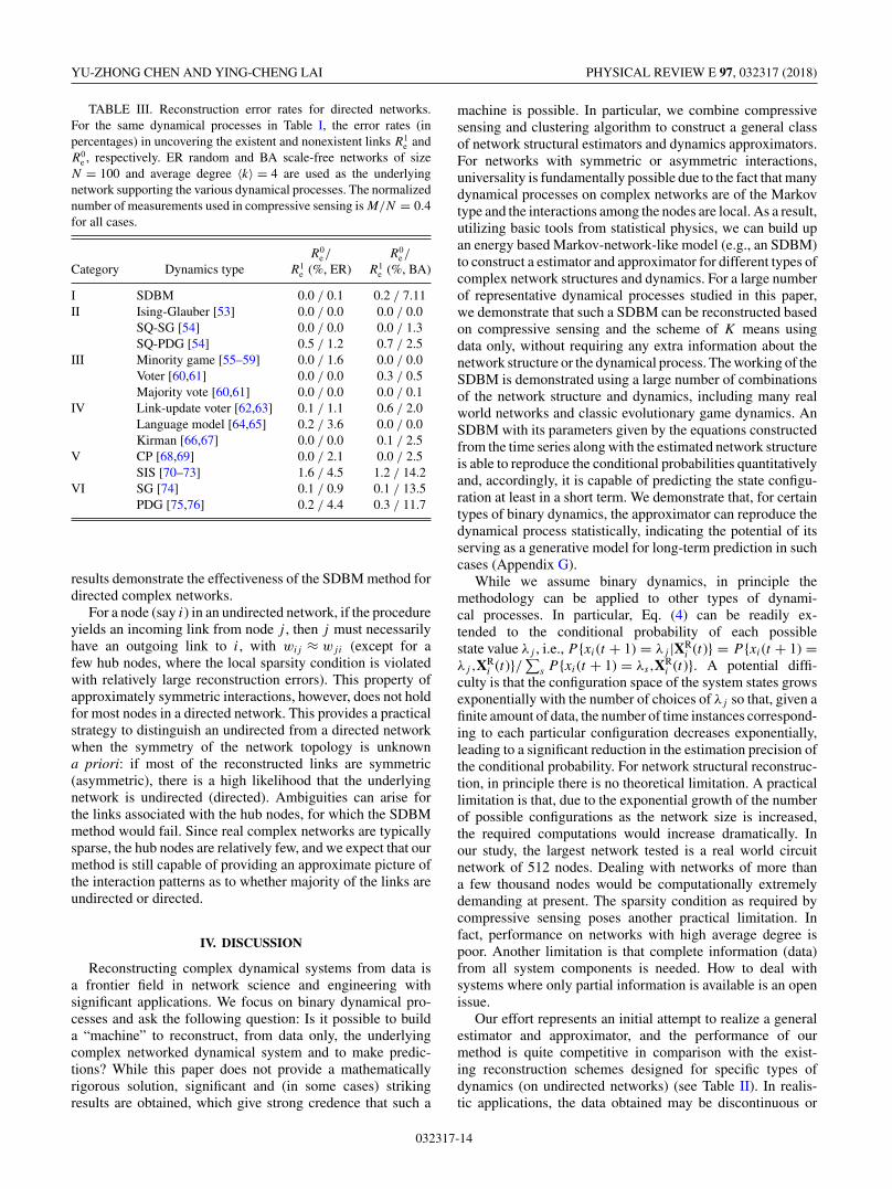
TABLE III. Reconstruction error rates for directed networks.For the same dynamical processes in Table I, the error rates (inpercentages) in uncovering the existent and nonexistent links R1

e andR0

e , respectively. ER random and BA scale-free networks of sizeN = 100 and average degree 〈k〉 = 4 are used as the underlyingnetwork supporting the various dynamical processes. The normalizednumber of measurements used in compressive sensing is M/N = 0.4for all cases.

R0e / R0

e /

Category Dynamics type R1e (%, ER) R1

e (%, BA)

I SDBM 0.0 / 0.1 0.2 / 7.11II Ising-Glauber [53] 0.0 / 0.0 0.0 / 0.0

SQ-SG [54] 0.0 / 0.0 0.0 / 1.3SQ-PDG [54] 0.5 / 1.2 0.7 / 2.5

III Minority game [55–59] 0.0 / 1.6 0.0 / 0.0Voter [60,61] 0.0 / 0.0 0.3 / 0.5Majority vote [60,61] 0.0 / 0.0 0.0 / 0.1

IV Link-update voter [62,63] 0.1 / 1.1 0.6 / 2.0Language model [64,65] 0.2 / 3.6 0.0 / 0.0Kirman [66,67] 0.0 / 0.0 0.1 / 2.5

V CP [68,69] 0.0 / 2.1 0.0 / 2.5SIS [70–73] 1.6 / 4.5 1.2 / 14.2

VI SG [74] 0.1 / 0.9 0.1 / 13.5PDG [75,76] 0.2 / 4.4 0.3 / 11.7

results demonstrate the effectiveness of the SDBM method fordirected complex networks.

For a node (say i) in an undirected network, if the procedureyields an incoming link from node j , then j must necessarilyhave an outgoing link to i, with wij ≈ wji (except for afew hub nodes, where the local sparsity condition is violatedwith relatively large reconstruction errors). This property ofapproximately symmetric interactions, however, does not holdfor most nodes in a directed network. This provides a practicalstrategy to distinguish an undirected from a directed networkwhen the symmetry of the network topology is unknowna priori: if most of the reconstructed links are symmetric(asymmetric), there is a high likelihood that the underlyingnetwork is undirected (directed). Ambiguities can arise forthe links associated with the hub nodes, for which the SDBMmethod would fail. Since real complex networks are typicallysparse, the hub nodes are relatively few, and we expect that ourmethod is still capable of providing an approximate picture ofthe interaction patterns as to whether majority of the links areundirected or directed.

IV. DISCUSSION

Reconstructing complex dynamical systems from data isa frontier field in network science and engineering withsignificant applications. We focus on binary dynamical pro-cesses and ask the following question: Is it possible to builda “machine” to reconstruct, from data only, the underlyingcomplex networked dynamical system and to make predic-tions? While this paper does not provide a mathematicallyrigorous solution, significant and (in some cases) strikingresults are obtained, which give strong credence that such a

machine is possible. In particular, we combine compressivesensing and clustering algorithm to construct a general classof network structural estimators and dynamics approximators.For networks with symmetric or asymmetric interactions,universality is fundamentally possible due to the fact that manydynamical processes on complex networks are of the Markovtype and the interactions among the nodes are local. As a result,utilizing basic tools from statistical physics, we can build upan energy based Markov-network-like model (e.g., an SDBM)to construct a estimator and approximator for different types ofcomplex network structures and dynamics. For a large numberof representative dynamical processes studied in this paper,we demonstrate that such a SDBM can be reconstructed basedon compressive sensing and the scheme of K means usingdata only, without requiring any extra information about thenetwork structure or the dynamical process. The working of theSDBM is demonstrated using a large number of combinationsof the network structure and dynamics, including many realworld networks and classic evolutionary game dynamics. AnSDBM with its parameters given by the equations constructedfrom the time series along with the estimated network structureis able to reproduce the conditional probabilities quantitativelyand, accordingly, it is capable of predicting the state configu-ration at least in a short term. We demonstrate that, for certaintypes of binary dynamics, the approximator can reproduce thedynamical process statistically, indicating the potential of itsserving as a generative model for long-term prediction in suchcases (Appendix G).

While we assume binary dynamics, in principle themethodology can be applied to other types of dynami-cal processes. In particular, Eq. (4) can be readily ex-tended to the conditional probability of each possiblestate value λj , i.e., P {xi(t + 1) = λj |XR

i (t)} = P {xi(t + 1) =λj ,XR

i (t)}/∑s P {xi(t + 1) = λs,XR

i (t)}. A potential diffi-culty is that the configuration space of the system states growsexponentially with the number of choices of λj so that, given afinite amount of data, the number of time instances correspond-ing to each particular configuration decreases exponentially,leading to a significant reduction in the estimation precision ofthe conditional probability. For network structural reconstruc-tion, in principle there is no theoretical limitation. A practicallimitation is that, due to the exponential growth of the numberof possible configurations as the network size is increased,the required computations would increase dramatically. Inour study, the largest network tested is a real world circuitnetwork of 512 nodes. Dealing with networks of more thana few thousand nodes would be computationally extremelydemanding at present. The sparsity condition as required bycompressive sensing poses another practical limitation. Infact, performance on networks with high average degree ispoor. Another limitation is that complete information (data)from all system components is needed. How to deal withsystems where only partial information is available is an openissue.

Our effort represents an initial attempt to realize a generalestimator and approximator, and the performance of ourmethod is quite competitive in comparison with the exist-ing reconstruction schemes designed for specific types ofdynamics (on undirected networks) (see Table II). In realis-tic applications, the data obtained may be discontinuous or

032317-14

SPARSE DYNAMICAL BOLTZMANN MACHINE FOR … PHYSICAL REVIEW E 97, 032317 (2018)

incomplete. In such cases, the short-term predictive powerpossessed by the estimator and approximator can be exploitedto overcome the difficulty of missing data, as the Markovnetwork nature of the SDBM makes backward inference pos-sible so that the system configurations during the time periodsof missing data may be inferred. When long-term predictionis possible, the approximator has the critical capability ofsimulating the system behavior and predicting the chancethat the system state enters into a global absorption phase,which may find significant applications such as disaster earlywarning. Another interesting reverse-engineering problem liesin the mapping between the original dynamics and the cor-responding parameter value distribution of the reconstructedSDBM. That is, a certain parameter distribution of the SDBMmay indicate a specific type of the original dynamics. Assuch, the correspondence can be used for precisely identifyingnonlinear and complex networked dynamical systems. It isalso possible to assess the relative importance of the nodesand links in a complex network based on their correspondingbiases and weights in the reconstructed SDBM for controllingthe network dynamics. These advantages justify our ideaof developing a machine for data-based reverse engineer-ing of complex networked dynamical systems, calling forfuture efforts in this emerging direction to further developand perfect the network structural estimator and dynamicsapproximator.

ACKNOWLEDGMENT

The authors would like to acknowledge financial supportfrom the Vannevar Bush Faculty Fellowship program spon-sored by the Basic Research Office of the Assistant Secretaryof Defense for Research and Engineering and funded by theOffice of Naval Research through Grant No. N00014-16-1-2828.

APPENDIX A: MODEL COMPLEXITYAND REPRESENTATION POWER

For dynamical processes in categories I and II, the transitionprobabilities P 0→1

i all have the form 1/[1 + exp(Ani + Bki)],where A and B are constants, and ni denotes the number ofnode i’s neighbors whose states are 1. We have

[1 + exp(Ani + Bki)]−1

={

1 + exp

[ki∑

m=1

wimxm(t) + bi

]}−1

,

which gives

ki∑m=1

Axm(t) + Bki =ki∑

m=1

wimxm(t) + bi. (A1)

In the ideal case where an absolutely accurate estimate ofP {xi(t + 1) = 1|XR

i (t)} can be obtained, Eq. (A1) holds for

any possible neighboring state configurations. We thus havewim = A and bi = Bki , and the probabilities conditioned onthese configurations sharing the same values of ni in theapproximator are all equal to P 0→1

i . This means that, in theory,the conditional probabilities can be reconstructed with zeroerrors. In fact, a one-to-one mapping between the coefficientsindicates that the model complexity of the SDBM provides theapproximator with sufficient representation power to modelthe dynamics processes in categories I and II. Practically, sincethe statistical estimations of P {xi(t + 1) = 1|XR

i (t)} may notbe absolutely identical under different neighboring configura-tions with the same values of ni due to random fluctuations, wehave wim ≈ A so that the conditional probabilities generatedby the approximator may differ from each other slightly andalso from the true probability P 0→1

i . As a result, randomrecovery errors can occur.For dynamical processes in categories other than I and II,the simple coefficient-mapping relation between the corre-sponding xm(t) terms on the two sides of Eq. (A1) becomenonlinear, due to the fact that the specific forms of P 0→1

i

differ substantially from that of the SDBM. In this case,each particular neighboring state configuration produces adistinct equation. There are 2ki equations in total, while thenumber of unknown variables to be solved is only ki + 1(wim for m = 1, . . . ,ki and bi). For ki � 2, there are thusmore equations than the number of unknown variables. As aresult, the representation power of the SDBM approximatoris limited by its finite model complexity so that, even inprinciple, the approximator may not be able to fully describethe original dynamical process. In our framework, we calculatethe Markov link weights and the node biases according to theki + 1 most frequently appeared neighboring state configura-tions. A consequence is that imprecise conditional probabilityestimations can arise for the configurations with relativelylower occurring frequency, giving rise to the nonzero peaksin the error distribution in Fig. 7. However, interestingly,with respect to the precision of the conditional probabilitiesproduced by the approximator, the SDBM parameters donot show a significantly strong preference towards the mostfrequently occurring configurations. In practice, the estimatedconditional probabilities for the majority of the less frequentlyoccurring configurations also fall within a close range ofthe true values. This phenomenon suggests the power of theapproximator to work beyond the limit set by its theoreticalmodel complexity. This is the main reason for the emergenceand persistence of the dominant peak at zero in the errordistribution.

APPENDIX B: JUSTIFICATIONFOR THE APPROXIMATION 〈ln Q〉 ≈ ln q

The approximation 〈ln Q〉 ≈ ln q is used in the maintext when deriving Eq. (9) from (7). For simplicity, wewrite P {xi(t + 1) = 1,XR

i (t)} as p1 in the following deriva-tion. For one particular state configuration (measurement) inEq. (7), we randomly shuffle all its similar configurationsand partition them into l buckets of the same size. Lettingln(1/p̃1

j − 1) denote the estimation of ln Q in bucket j , we

032317-15

YU-ZHONG CHEN AND YING-CHENG LAI PHYSICAL REVIEW E 97, 032317 (2018)

have

〈ln Q〉 = 7

⟨ln

(1

p1− 1

)⟩=

∑lj=1 ln

(1/p̃1

j − 1)

l

= ln l

√√√√ l∏j=1

(1

p̃1j

− 1

)� ln

⎡⎣1

l

l∑j=1

(1

p̃1j

− 1

)⎤⎦

= ln

[⟨1

p1

⟩− 1

], (B1)

where the equality holds if all the summation elements haveequal values, so the geometrical and algebraic means are thesame. When there are a sufficiently large number of similarconfigurations in each bucket, we have

p̃11 ≈ p̃1

2 ≈ p̃13 ≈ . . . ≈ p̃1

l ≈ 〈x(t + 1)〉 (B2)

and thus1

p̃11

≈ 1

p̃12

≈ 1

p̃13

≈ . . . ≈ 1

p̃1l

≈ 1

〈x(t + 1)〉 , (B3)

so that the equal sign in Eq. (B1) holds. Accordingly, wehave 〈ln Q〉 ≈ ln[〈 1

p1 〉 − 1]. Using supplemental Eqs. (B2) and(B3), we obtain⟨

1

p1

⟩= 1

l

l∑j=1

1

p1j

≈ 1

〈x(t + 1)〉 . (B4)

Consequently, we have ln Q ≈ 〈ln Q〉 ≈ ln q.This approximation can be further justified empirically. We

have calculated ln q versus 〈ln Q〉 for a wide range of thebucket size and found that, for different bucket size, the distri-butions all concentrate on the diagonal line with insignificantvariances, indicating the effectiveness and accuracy of ourapproximation. Similar results have been obtained, regardlessof network topology and dynamics property. We note that asimilar approximation method was used by Shen et al. in theirwork of reconstruction of propagation networks from binarydata [28].

APPENDIX C: IMPLEMENTATION DETAILS OF 14DYNAMICAL PROCESSES ON COMPLEX NETWORKS

All types of network dynamical processes studied in themain text, except for PDG and SG, are implemented in thefollowing way. At each time step t , the probabilities for nodei to have a state xi(t + 1) = 1 and 0 at the next time stepconditioned on the state configuration of i’s neighbors, i.e.,P 0→1

i and P 1→0i , are calculated according to Table I in the main

text. If xi(t) = 0 (or 1), then it is switched to state xi(t + 1) = 1(or 0) with the probability P 0→1

i (or P 1→0i ) or remains at 0 (or

1) with the probability 1 − P 0→1i (or 1 − P 1→0

i ).Listed below is a detailed description of the dynamical

processes and the parameter settings. (Reasonable changesin parameter values do not affect the reconstruction perfor-mance.)

SDBM. The dynamics is described in detail in the maintext. The network parameters (link weights and node biases)are uniformly chosen between 0.3 and 0.7 in our calculation.

Ising-Glauber. Opinion dynamics models often adoptthe classic Ising model of ferromagnetic spins [53]. The

temperature parameter κ characterizes the level of “rational-ity” of the individuals, which represents the uncertainties inaccepting the opinion. The coupling strength parameter J

(or the ferromagnetic-interaction parameter) characterizes theintensity of the interaction between the connected nodes. Thesimulation parameters are κ = 1 and J = 0.1.

Majority vote. The majority-vote model [60,61] is anonequilibrium spin model. Spins tend to align with theneighborhood majority under the influence of noise withparameter Q quantifying the probability of misalignment. Inour simulations, we set Q = 0.3.

Minority game. In the minority game model [55–59], eachindividual chooses the strategy adopted by the minority of itsneighbors with a higher probability than that for the majority.The probability for node i to be 1 at the next time step isproportional to the number of its 0-state neighbors, ki − ni .We then have P 0→1

i = (ki − ni)/ki and P 1→0i = ni/ki .

Voter and link-update voter. In the voter model [60,82],each node i adopts the state of one of its randomly selectedneighbors. If i is currently inactive (state 0), while there are ni

neighbors in the active state (state 1), it becomes active with theprobability P 0→1

i = ni/ki . An active node i becomes inactivewith the probability P 1→0

i = (ki − ni)/ki . The voter model issimilar to the minority game model but with the definition ofP 0→1

i and P 1→0i swapped. The link-update voter model is a

variant of the voter model [62,63].Language model. In the language model [64,65], the 0

and 1 states stand for an individual’s two primary choicesof the language. The probability of switching language isproportional to the fraction of the speakers in its neighborhood,raised to the power α and multiplied by the status parameter s

or 1 − s of the respective language. In our simulations, we useα = 0.5 and s = 0.6.

Kirman ant colony model. In the model [66,67], to choosebetween stock market trading strategies, nodes move fromthe nonadopted state (state 0) to the adopted state (state 1)with the probability P 0→1

i = c1 + dni , where c1 represents theindividual strategy, which is independent of the influence of itsneighbors. The parameter d quantifies the herding behavior,whereby a nonadopted-state individual copies the strategy oftheir ni adopted-state neighbors. A node i with ni of its ki

neighbors in the adopted state has ki − ni neighbors in thenonadopted state. Due to the herding effect, the probabilityfor the transition from an adopted state to a nonadoptedstate is P 1→0

i = c2 + d(ki − ni). In our simulations, we setc1 = c2 = 0.1 and d = 10/N , where N is the network size.

SIS and CP. In the susceptible-infected-susceptible (SIS)disease-spread model [70,72,83], an infected individual trans-mits disease to node i in its neighborhood with the probabilityλi . If a susceptible node i has ni infected neighbors, theprobability that it will be infected is P 0→1

i . The recoveryrate P 1→0

i = μi is kept constant for node i. When simulatingthe SIS model, all infected neighbors of node i affect i. Inparticular, for each infected neighbor, a random number isdrawn and checked if it is smaller than λi , and i gets infectedif any of the random numbers are smaller than λi . We thushave P 0→1

i = 1 − (1 − λ)ni , where the second term gives thechance for i to remain susceptible.

For the contact process (CP) model [68,69], at a time step,each node i randomly selects one of its ki neighbors and checks

032317-16

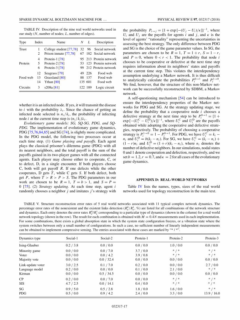
SPARSE DYNAMICAL BOLTZMANN MACHINE FOR … PHYSICAL REVIEW E 97, 032317 (2018)

TABLE IV. Description of the nine real world networks used inour study (N , number of nodes; L, number of edges).

Type Index Name N L Description

Trust 1 College student [77,78] 32 96 Social network2 Prison inmate [77,78] 67 182 Social network

4 Protein-1 [78] 95 213 Protein networkProtein 5 Protein-2 [78] 53 123 Protein network

6 Protein-3 [78] 99 212 Protein network

12 Seagrass [79] 49 226 Food webFood web 13 Grassland [80] 88 137 Food web

14 Ythan [80] 135 601 Food web

Circuits 3 s208a [81] 122 189 Logic circuit

whether it is an infected node. If yes, it will transmit the diseaseto i with the probability λi . Since the chance of getting aninfected node selected is ni/ki , the probability of infectingnode i at the current time step is (ni/ki)λi .

Evolutionary game models: SG, SQ-SG, PDG, and SQ-PDG. The implementation of evolutionary game dynamics,PDG [75,76,84,85] and SG [74], is slightly more complicated.In the PDG model, the following two processes occur ateach time step. (1) Game playing and payoffs. Each agentplays the classical prisoner’s dilemma game (PDG) with allits nearest neighbors, and the total payoff is the sum of thepayoffs gained in its two-player games with all the connectedagents. Each player may choose either to cooperate, C, orto defect, D, in a single encounter. If both players chooseC, both will get payoff R. If one defects while the othercooperates, D gets T , while C gets S. If both defect, bothget P , where T > R > P > S. The PDG parameters in ourwork are chosen to be R = 1, T = b > 1, and S = P =0 [75]. (2) Strategy updating. At each time step, agent i

randomly chooses a neighbor j and imitates j ’s strategy with

the probability Pi→j = {1 + exp [−(Uj − Ui)/κ]}−1, whereUi and Uj are the payoffs for agents i and j , and κ is thelevel of agents’ “rationality” representing the uncertainties inassessing the best strategy. The only difference between PDGand SG is the choice of the game parameter values. In SG, theparameters are chosen to be R = 1, T = 1 + r , S = 1 − r ,and P = 0, where 0 < r < 1. The probability that node i

chooses to be cooperative or defective at the next time steprequires information about its neighbors’ states and payoffsat the current time step. This violates the interdependencyassumption underlying a Markov network. It is thus difficultto analytically calculate the probabilities P 0→1

i and P 1→0i .

We find, however, that the structure of this non-Markov net-work can be successfully reconstructed by SDBM, a Markovnetwork.

A self-questioning mechanism [54] can be introduced toensure the interdependency properties of the Markov net-works for PDG and SG. At the strategy updating stage, wedefine the probability that a cooperative node i chooses adefective strategy at the next time step to be P 0→1

i = {1 +exp [−(UC

i − UDi )/κ]}−1, where UC

i and UDi are the payoffs

obtained while adopting the cooperative and defective strate-gies, respectively. The probability of choosing a cooperativestrategy is P 1→0

i = 1 − P 0→1i . For PDG, we have UC

i = ki −ni and UD

i = b(ki − ni). For SG, we have UCi = (ki − ni) +

(1 − r)ni and UDi = (1 + r)(ki − ni), where ni denotes the

number of defective neighbors. In our simulations, nodal states0 and 1 denote cooperation and defection, respectively, and weset b = 1.2, r = 0.7, and κ = 2 for all cases of the evolutionarygame dynamics.

APPENDIX D: REAL-WORLD NETWORKS

Table IV lists the names, types, sizes of the real worldnetworks used for topology reconstruction in the main text.

TABLE V. Structure reconstruction error rates of 5 real world networks associated with 11 typical complex network dynamics. Thepercentage error rates of the nonexistent and the existent links detection (R0

e /R1e , %) are listed for all combinations of the network structure

and dynamics. Each entry denotes the error rates R0e /R1

e corresponding to a particular type of dynamics (shown in the column) for a real worldnetwork topology (shown in the row). The result for each combination is obtained with M = 0.4N measurements used in each implementation.For some combinations, there exists a global absorption state in which the system state configuration freezes, or a vibration state where thesystem switches between only a small number of configurations. In such a case, no sufficient number of linearly independent measurementscan be obtained to implement compressive sensing. The entries associated with these cases are marked by “* / *”.

Dynamics type Social-1 Social-2 Protein-1 Protein-2 Protein-3

Ising-Glauber 0.2 / 3.8 0.0 / 0.0 0.0 / 0.0 1.0 / 0.0 0.0 / 0.0

Minority game 0.0 / 0.0 0.0 / 7.0 3.7 / 0.0 * / * * / *Voter 0.0 / 0.0 0.0 / 4.2 3.9 / 0.8 * / * * / *Majority vote 0.0 / 0.0 0.0 / 32.4 0.0 / 0.0 0.0 / 0.0 0.0 / 0.0

Link-update voter 3.0 / 2.5 0.1 / 7.0 0.2 / 0.0 0.0 / 0.0 2.7 / 0.0Language model 0.2 / 0.0 0.0 / 0.0 0.1 / 0.0 2.1 / 0.0 * / *Kirman 0.0 / 0.0 0.5 / 34.5 0.0 / 0.0 0.0 / 0.0 0.0 / 0.0

CP 0.2 / 0.0 0.0 / 7.0 0.0 / 0.0 * / * * / *SIS 4.7 / 2.5 0.0 / 14.1 0.4 / 0.0 * / * * / *

SG 0.9 / 5.0 0.5 / 2.8 1.8 / 0.0 1.6 / 0.0 * / *PDG 0.5 / 0.0 0.9 / 4.2 2.4 / 0.0 3.3 / 0.0 13.9 / 16.0

032317-17

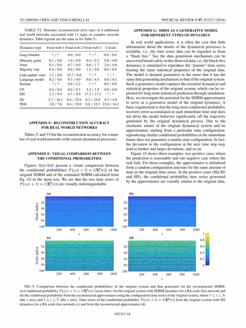
YU-ZHONG CHEN AND YING-CHENG LAI PHYSICAL REVIEW E 97, 032317 (2018)

TABLE VI. Structure reconstruction error rates of 4 additionalreal world networks associated with 11 types of complex networkdynamics. Table legends are the same as for Table V.

Dynamics type Food web-1 Food web-2 Food web-3 Circuit

Ising-Glauber * / * 0.0 / 0.0 * / * 0.0 / 0.0

Minority game 0.1 / 0.0 1.0 / 0.0 0.4 / 0.3 0.8 / 0.0Voter 0.1 / 0.0 0.7 / 0.0 0.6 / 1.7 2.0 / 0.0Majority vote 0.4 / 0.0 0.0 / 0.0 1.5 / 0.0 0.0 / 0.0

Link-update voter 1.1 / 0.0 15.7 / 0.0 * / * * / *Language model 0.2 / 0.0 0.3 / 0.0 0.0 / 4.4 0.0 / 0.1Kirman * / * 0.0 / 2.2 * / * 0.0 / 0.0

CP 0.4 / 0.5 0.0 / 0.7 5.3 / 1.5 0.0 / 0.0SIS 1.3 / 9.4 4.7 / 8.0 17.3 / 17.3 * / *

SG 2.1 / 16.1 8.4 / 25.6 6.2 / 23.0 8.3 / 4.8PDG 2.8 / 7.6 8.4 / 19.0 8.8 / 15.3 23.0 / 14.3

APPENDIX E: RECONSTRUCTION ACCURACYFOR REAL WORLD NETWORKS

Tables V and VI list the reconstruction accuracy for a num-ber of real world networks with various dynamical processes.

APPENDIX F: VISUAL COMPARISON BETWEENTHE CONDITIONAL PROBABILITIES

Figures 9(a)–9(d) present a visual comparison betweenthe conditional probabilities P {xi(t + 1) = 1|XR

i (t)} of theoriginal SDBM and of the estimated SDBM calculated fromEq. (5) in the main text. We see that the two time series ofP {xi(t + 1) = 1|XR

i (t)} are visually indistinguishable.

APPENDIX G: SDBM AS A GENERATIVE MODELFOR DIFFERENT TYPES OF DYNAMICS

In real world applications, it is often the case that littleinformation about the details of the dynamical processes isavailable, i.e., the time series data can be regarded as froma “black box.” Say the data generation mechanism can beuncovered based solely on the observed data, i.e., the black-boxdynamics is simulated to reproduce the “pseudo”-time seriesbearing the same statistical properties of the original data.The model is deemed generative in the sense that it has thesame data generating mechanism as that of the original system.Such a generative model captures the essential dynamical andstatistical properties of the original system, which can be ex-ploited for long-term statistical prediction through simulation.Here, we investigate the potential for the SDBM approximatorto serve as a generative model of the original dynamics. Abasic requirement is that the long-term conditional probabilityrecovery error accumulated at each immediate time step doesnot drive the model behavior significantly off the trajectorygenerated by the original dynamical process. Due to thestochastic nature of the original dynamical system and itsapproximator, starting from a particular state configuration,reproducing similar conditional probabilities in the immediatefuture does not guarantee a similar state configuration. In fact,the deviation in the configuration at the next time step maylead to further and larger deviations, and so on.

Figure 10 shows three examples: two positive cases wherethe prediction is reasonable and one negative case where thetask fails. For those examples, the approximator is initializedfrom a random configuration and runs for the same amount oftime as the original time series. In the positive cases (SQ-SGand SIS), the conditional probability time series generatedby the approximator are visually similar to the original data,

FIG. 9. Comparison between the conditional probabilities of the original system and that generated via the reconstructed SDBM.(a) Conditional probability P {xi(t + 1) = 1|XR

i (t)} versus time t for the original system with SDBM dynamics for a BA scale-free network and(b) the conditional probability from the reconstructed approximator using the configuration time series of the original system, where 1 � i � N

(the y axis) and 1 � t � T (the x axis). Time series of the conditional probability P {xi(t + 1) = 1|XRi (t)} from the original system with SIS

dynamics for a BA scale-free network (c) and from the reconstructed approximator (d).

032317-18

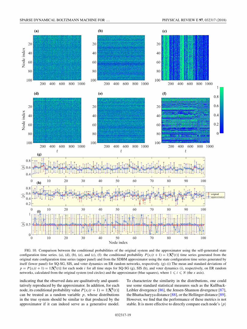
SPARSE DYNAMICAL BOLTZMANN MACHINE FOR … PHYSICAL REVIEW E 97, 032317 (2018)

FIG. 10. Comparison between the conditional probabilities of the original system and the approximator using the self-generated stateconfiguration time series. (a), (d), (b), (e), and (c), (f): the conditional probability P {xi(t + 1) = 1|XR

i (t)} time series generated from theoriginal state configuration time series (upper panel) and from the SDBM approximator using the state configuration time series generated byitself (lower panel) for SQ-SG, SIS, and voter dynamics on ER random networks, respectively. (g)–(i) The mean and standard deviations ofp = P {xi(t + 1) = 1|XR

i (t)} for each node i for all time steps for SQ-SG (g), SIS (h), and voter dynamics (i), respectively, on ER randomnetworks, calculated from the original system (red circles) and the approximator (blue squares), where 1 � i � N (the x axis).

indicating that the observed data are qualitatively and quanti-tatively reproduced by the approximator. In addition, for eachnode, its conditional probability value P {xi(t + 1) = 1|XR

i (t)}can be treated as a random variable p, whose distributionsin the true system should be similar to that produced by theapproximator if it can indeed serve as a generative model.

To characterize the similarity in the distributions, one coulduse some standard statistical measures such as the Kullback-Leibler divergence [86], the Jensen-Shannon divergence [87],the Bhattacharyya distance [88], or the Hellinger distance [89].However, we find that the performance of these metrics is notstable. It is more effective to directly compare each node’s 〈p〉

032317-19

YU-ZHONG CHEN AND YING-CHENG LAI PHYSICAL REVIEW E 97, 032317 (2018)

and p values from the original data and the approximator,e.g., for the three examples shown in Figs. 10(c), 10(f), and10(i). The result is that, except for a few nodes, the valuesof 〈p〉 and p obtained from the data and SDBM agree witheach other for the two positive cases, but there is a substantialdifference for the negative case. Our calculation also showsthat there are cases where the approximator reproduces similarvalues of 〈p〉 and p for a substantial fraction of the nodesin the network, but with deviations for the remaining nodes.We conclude that the SDBM approximator can serve as agenerative model for some systems. Improvement is necessaryto generalize the generative power of SDBM.

We have also carried out a comparison study between theconditional probabilities of the original system and of theapproximator using its self-generated state configuration timeseries for all types of dynamics studied except for the non-Markovian classic PDG and SG, whose conditional probabilitytime series are difficult to compute. We find that in abouthalf of the cases, namely, SDBM itself, Ising-Glauber, SQ-SG,SQ-PDG, the Kirman model, CP, and SIS, the reconstructedSDBM approximators are capable of serving as a generativemodel of the original time series data, so the reconstructedSDBMs can be used to simulate the long-term behavior of thecorresponding original systems.

[1] S. Grün, M. Diesmann, and A. Aertsen, Neural Comput. 14, 43(2002).

[2] S. Grün, A. Aertsen, and S. Rotter, Neural Comput. 14, 121(2002).

[3] G. Pipa and S. Grün, Neurocomputing 52-54, 31 (2003).[4] T. S. Gardner, D. di Bernardo, D. Lorenz, and J. J. Collins,

Science 301, 102 (2003).[5] M. Bansal, V. Belcastro, A. Ambesi-Impiombato, and D. di

Bernardo, Mol. Syst. Biol. 3, 78 (2007).[6] F. Geier, J. Timmer, and C. Fleck, BMC Syst. Biol. 1, 11 (2007).[7] K. Supekar, V. Menon, D. Rubin, M. Musen, and M. D. Greicius,

PLoS Comput. Biol. 4, e1000100 (2008).[8] M. Hecker, S. Lambeck, S. Toepferb, E. van Someren, and R.

Guthke, BioSystems 96, 86 (2009).[9] T. Tanaka, Phys. Rev. E 58, 2302 (1998).

[10] S. Cocco and R. Monasson, Phys. Rev. Lett. 106, 090601 (2011).[11] E. Aurell and M. Ekeberg, Phys. Rev. Lett. 108, 090201 (2012).[12] H. C. Nguyen and J. Berg, Phys. Rev. Lett. 109, 050602 (2012).[13] F. Ricci-Tersenghi, J. Stat. Mech. (2012) P08015.[14] Y. Roudi and J. Hertz, Phys. Rev. Lett. 106, 048702 (2011).[15] M. Méard and J. Sakellariou, J. Stat. Mech. (2011) P08015.[16] J. Sohl-Dickstein, P. B. Battaglino, and M. R. DeWeese, Phys.

Rev. Lett. 107, 220601 (2011).[17] P. Zhang, J. Stat. Phys. 148, 502 (2012).[18] H.-L. Zeng, M. Alava, E. Aurell, J. Hertz, and Y. Roudi, Phys.

Rev. Lett. 110, 210601 (2013).[19] L. Barnett, J. T. Lizier, M. Harré, A. K. Seth, and T. Bossomaier,

Phys. Rev. Lett. 111, 177203 (2013).[20] A. Decelle and F. Ricci-Tersenghi, Phys. Rev. Lett. 112, 070603

(2014).[21] M. Timme, Phys. Rev. Lett. 98, 224101 (2007).[22] J. Bongard and H. Lipson, Proc. Natl. Acad. Sci. USA 104, 9943

(2007).[23] S. G. Shandilya and M. Timme, New J. Phys. 13, 013004 (2011).[24] A. Clauset, C. Moore, and M. E. J. Newman, Nature (London)

453, 98 (2008).[25] Z. Levnajić and A. Pikovsky, Phys. Rev. Lett. 107, 034101

(2011).[26] W.-X. Wang, R. Yang, Y.-C. Lai, V. Kovanis, and M. A. F.

Harrison, Europhys. Lett. 94, 48006 (2011).[27] W.-X. Wang, Y.-C. Lai, C. Grebogi, and J.-P. Ye, Phys. Rev. X

1, 021021 (2011).[28] Z. Shen, W.-X. Wang, Y. Fan, Z. Di, and Y.-C. Lai, Nat. Commun.

5, 4323 (2014).

[29] X. Han, Z. Shen, W.-X. Wang, and Z. Di, Phys. Rev. Lett. 114,028701 (2015).

[30] W. Pan, Y. Yuan, J. Goncalves, and G.-B. Stan, IEEE Trans.Autom. Control 61, 182 (2016).

[31] W. Pan, A. Sootla, and G.-B. Stan, IEEE Proc. 47, 3208(2014).

[32] S. L. Brunton, J. L. Proctor, and J. N. Kutz, Proc. Natl. Acad.Sci. USA 113, 3932 (2016).

[33] A. M. and J. Goncalves, in 2016 IEEE 55th Conference onDecision and Control (CDC) (IEEE, Piscataway, NJ, 2016),pp. 6500–6506.

[34] J. Li, Z. Shen, W.-X. Wang, C. Grebogi, and Y.-C. Lai, Phys.Rev. E 95, 032303 (2017).

[35] C. Ma, H.-S. Chen, Y.-C. Lai, and H.-F. Zhang, Phys. Rev. E 97,022301 (2018).

[36] W.-X. Wang, Q. Chen, L. Huang, Y.-C. Lai, and M. A. F.Harrison, Phys. Rev. E 80, 016116 (2009).

[37] J. Ren, W.-X. Wang, B. Li, and Y.-C. Lai, Phys. Rev. Lett. 104,058701 (2010).

[38] C. M. Bishop, Pattern Recognition and Machine Learning(Springer, Berlin, 2006).

[39] S. Russell and P. Norvig, Artificial Intelligence: A ModernApproach, 3rd ed. (Prentice Hall, Englewood Cliffs, NJ, 2009).

[40] D. H. Ackley, G. E. Hinton, and T. J. Sejnowski, Cogn. Sci. 9,147 (2014).

[41] E. J. Candès, J. K. Romberg, and T. Tao, IEEE Trans. Inf. Theory52, 489 (2006).

[42] E. J. Candes, J. K. Romberg, and T. Tao, Commun. Pure Appl.Math. 59, 1207 (2006).

[43] D. L. Donoho, IEEE Trans. Inf. Theory 52, 1289 (2006).[44] R. G. Baraniuk, IEEE Sig. Proc. Mag. 24, 118 (2007).[45] E. J. Candès and M. B. Wakin, IEEE Sig. Proc. Mag. 25, 21

(2008).[46] J. Romberg, IEEE Sig. Proc. Mag. 25, 14 (2008).[47] R.-Q. Su, X. Ni, W.-X. Wang, and Y.-C. Lai, Phys. Rev. E 85,

056220 (2012).[48] R.-Q. Su, W.-X. Wang, and Y.-C. Lai, Phys. Rev. E 85,

065201(R) (2012).[49] R.-Q. Su, Y.-C. Lai, X. Wang, and Y.-H. Do, Sci. Rep. 4, 3944

(2014).[50] V. Kishore, M. S. Santhanam, and R. E. Amritkar, Phys. Rev.

Lett. 106, 188701 (2011).[51] Y.-Z. Chen, Z.-G. Huang, and Y.-C. Lai, Sci. Rep. 4, 06121

(2014).

032317-20

SPARSE DYNAMICAL BOLTZMANN MACHINE FOR … PHYSICAL REVIEW E 97, 032317 (2018)

[52] Y.-Z. Chen, Z.-G. Huang, H.-F. Zhang, D. Eisenberg,T. P. Seager, and Y.-C. Lai, Sci. Rep. 5, 17277(2015).

[53] R. J. Glauber, J. Math. Phys. (NY) 4, 294 (1963).[54] K. Gao, W.-X. Wang, and B.-H. Wang, Phys. A (Amsterdam)

380, 528 (2007).[55] D. Challet and Y.-C. Zhang, Phys. A (Amsterdam) 246, 407

(1997).[56] D. Challet, M. Marsili, and Y.-C. Zhang, Minority Games:

Interacting Agents in Financial Markets (Oxford UniversityPress, Oxford, 2005).

[57] M. Paczuski, K. E. Bassler, and A. Corral, Phys. Rev. Lett. 84,3185 (2000).

[58] T. Zhou, B.-H. Wang, P.-L. Zhou, C.-X. Yang, and J. Liu, Phys.Rev. E 72, 046139 (2005).

[59] Z.-G. Huang, J.-Q. Zhang, J.-Q. Dong, L. Huang, and Y.-C. Lai,Sci. Rep. 2, 703 (2012).

[60] T. M. Liggett, Interacting Particle Systems (Springer, New York,1985).

[61] M. J. de Oliveira, J. Stat. Phys. 66, 273 (1992).[62] A. Barrat, M. Barthélemy, and A. Vespignani, Dynamical

Processes on Complex Networks (Cambridge University Press,Cambridge, England, 2008).

[63] C. Castellano, S. Fortunato, and V. Loreto, Rev. Mod. Phys. 81,591 (2009).

[64] F. Vazquez, X. Castelló, and M. S. Miguel, J. Stat. Mech. (2010)P04007.

[65] D. M. Abrams and S. H. Strogatz, Nature (London) 424, 900(2003).

[66] A. Kirman, Quarterly J. Econom. 108, 137 (1993).[67] S. Alfarano, T. Lux, and F. Wagner, Comput. Econom. 26, 19

(2005).[68] C. Castellano and R. Pastor-Satorras, Phys. Rev. Lett. 96, 038701

(2006).

[69] E. Volz and L. A. Meyers, J. R. Soc. Interface 6, 233 (2009).[70] N. T. J. Bailey, The Mathematical Theory of Infectious Diseases

(Griffin, London, 1975).[71] R. M. Anderson and R. M. May, Infectious Diseases in Humans

(Oxford University Press, Oxford, England, 1992).[72] R. Pastor-Satorras and A. Vespignani, Phys. Rev. Lett. 86, 3200

(2001).[73] R. Pastor-Satorras and A. Vespignani, Phys. Rev. E 63, 066117

(2001).[74] R. Sugden, The Economics of Rights Co-operation and Welfare

(Blackwell, Oxford, UK, 1986).[75] R. Axelrod and W. D. Hamilton, Science 211, 1390 (1981).[76] G. Szabó and C. Tőke, Phys. Rev. E 58, 69 (1998).[77] M. A. J. V. Duijn, M. Huisman, F. N. Stokman, F. W. Wasseur,

and E. P. H. Zeggelink, J. Math. Sociol. 27, 153 (2003).[78] R. Milo, S. Itzkovitz, N. Kashtan, R. Levitt, S. Shen-Orr, I.

Ayzenshtat, M. Sheffer, and U. Alon, Science 303, 1538 (2004).[79] R. R. Christian and J. J. Luczkovich, Ecol. Modell. 117, 99

(1999).[80] J. A. Dunne, R. J. Williams, and N. D. Martinez, Proc. Natl.

Acad. Sci. USA 99, 12917 (2002).[81] R. Milo, S. Shen-Orr, S. Itzkovitz, N. Kashtan, D. Chklovskii,

and U. Alon, Science 298, 824 (2002).[82] V. Sood and S. Redner, Phys. Rev. Lett. 94, 178701 (2005).[83] P. J. Antsaklis and A. N. Michel, Linear Systems (McGraw-Hill,

New York, 1997).[84] Y.-Z. Chen, Z.-G. Huang, S.-J. Wang, Y. Zhang, and Y.-H. Wang,

Phys. Rev. E 79, 055101(R) (2009).[85] Y.-Z. Chen and Y.-C. Lai, Phys. Rev. E 86, 045101(R) (2012).[86] S. Kullback and R. A. Leibler, Ann. Math. Stat. 22(1), 79 (1951).[87] J. Burbea and C. R. Rao, IEEE Trans. Inf. Theory 28, 489 (1982).[88] A. Bhattacharyya, Sankhyã: Indian J. Stat. 7, 401 (1946).[89] E. Hellinger, J. für die reine und angewandte Math. (Crelle’s

Journal) 136, 210 (1909).

032317-21