Embed Size (px)
Citation preview

1
Space weather and its relevance to Indonesia
Simon Wing
The Johns Hopkins University
Applied Physics Laboratory

2
outline
1. What is space weather?
2. Space weather effects on satellite
communication:
a. polar region
b. equatorial region
3. Space weather forecasting with machine learning
• Kp forecast models
• Solar cycle dependence of Kp forecasts
4. Summary

3
1. What is space weather?

4
What is space weather?
Space weather refers to conditions on the sun, in
solar wind, and in the Earth’s magnetosphere,
ionosphere, and thermosphere that can influence
the performance and reliability of space-borne
and ground-based technological systems and
can endanger human life or health.
[The National Space Weather Program Strategic Plan, FCM-P30-1995,
Washington D.C., 1995]

5
Divisions of The Johns Hopkins University
School of Arts & Sciences
Whiting School of Engineering
School of Professional Studies
in Business & Education
School of Hygiene & Public Health
School of Medicine
School of Nursing
Applied
Physics Laboratory
Nitze School of Advanced
International Studies (SAIS)
Peabody Institute
6
JHU/APL & Space:
“From the Sun to Pluto -- and Beyond”
Sun
Venus Earth Uranus Saturn Jupiter Asteroid
and Comet
Moon
Mars Pluto Neptune
NEAR Voyager
Galileo
New
Horizons
JUNO
Voyager
Cassini
Voyager New
Horizons
Ulysses
ACE
STEREO
MESSENGER Voyager MagSat
Geosat
PolarBear
Hilat
GEOS-A
Grace
TIMED
MMS
MSX
NIMS
MRO
Mercury
Apollo 17
Chandrayaan
LRO
since 1958:
64 spacecraft
150+ payloads

7

8

9
some of the phenomena affected by space weather

Increasing reliance on space weather

11
Snapshot of some space weather products covering the region from the Sun to Earth

12
* Product has been transitioned to AFWA
Examples of space weather products that are available in realtime
*
*
*
*
*
*
#
# Product is being transitioned to NOAA and AFRL

13
Radiation Belt Storm Probes
(RBSP)
Impacts:
1. Understand fundamental particle
radiation processes operating
throughout the universe.
2. Understand Earth’s particle
radiation belts and related
regions that pose hazards to
human and robotic explorers.
Objective:
Provide understanding, ideally to the point of
predictability, of how populations of relativistic electrons
and penetrating ions in space form or change in
response to variable inputs of energy from the Sun.
Intensities of Earth’s dynamic
radiation belts
a huge space weather component

14
RBSP launched Aug 30, 2012

Spacecraft charging

16
Space weather research
• Most space weather research traditionally has
focused on high latitude phenomena
• There are still a lot of unknowns at low latitude
• There are lots of opportunities for country like
Indonesia to contribute

17
2. Space weather effects on satellite
communication
a. Polar region
b. Equatorial region

PALAPA-B Satellites
• Palapa-B covered equatorial region • Owned by Indonesia's state-owned telecommunications company,
TELKOM
Motivations
• GPS is now widely used all over the world, including
Indonesia
• Indonesia has owned Palapa series communication
satellites for almost 4 decades

One-Way VSAT
• Using technology like VSAT, Palapa can provide communication in remote and rural areas

Two-Way VSAT
• Useful for education in areas without phone lines
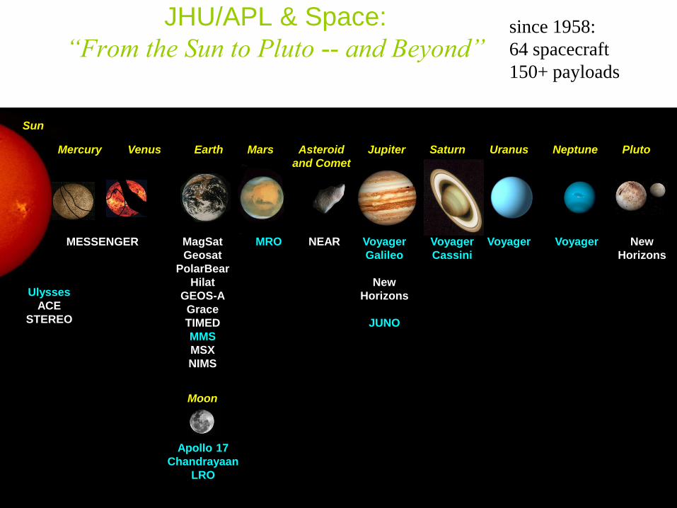
PALAPA-C
• C1 Launched Jan 1996, C2 Launched May 1996
• Unfolds to 21m in length, Solar panals provide 3700 W of power
• Still in service today
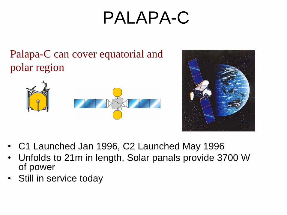
Palapa-C can cover equatorial and
polar region
PALAPA-C Coverage
Palapa-C covers a wider geographical area, including polar region
such as Southern Australia and New Zealand, which has its own
challenges

Two primary ionospheric regions that can disrupt satellite communications:
SAT COM
AURORAL IRREGULARITIES
GPS
PLASMA BUBBLES
GPS
SAT COM
MAGNETIC
EQUATOR
DAY NIGHT
EQUATORIAL F LAYER
ANOMALIES
SBR
POLAR CAP
PATCHES
a. Polar region: auroral particle precipitation
b. Equatorial region: plasma bubble

Scintillation The Problem
• Ionospheric density gradients can distort satellite
communication or radar signal traversing it to/from a satellite
or target
Sat com
Receiver
Radar
Receiver
Ionosphere
Ionospheric Scintillation
Aurora pp or Bubbles

25

26
a. Polar region: Auroral particle
precipitation
2. Space weather effects on
satellite communication

27
Aurora
vicinity of Fairbanks, Alaska (by Jan Curtis)

aurora seen from the ground

29
UV image of auroral oval (in false
colors)
The Earth has a “halo” above north and
south pole that is known as auroral oval
• Aurora is related to the activities of the
Sun
• Aurora is an ionospheric emission due
to particle precipitation
• The particles originate from the sun
or/and magnetotail and follow the
magnetic field line to the ionosphere


The aurora seen from space
on the
dayside
aurora is
harder to
see

aurora dynamics shown in movie taken from space

Global MHD simulations showing aurora dynamics

Northern and Southern light

Input:
DMSP SSJ4, UAF Meridian Scanning Photometer (MSP), SuperDARN radar
Output
Auroral oval location and intensity for both the northern and southern hemispheres,
polar cap fluxes
X : DMSP boundaries
R : SuperDARN boundaries
P: MSP boundaries
r : SuperDARN upper-limit of the
equatorward boundary position.
Intensity scale: log10 eV/cm2 s str.
(Auroral) Oval Variation, Assessment, Tracking,
Intensity, and Online Nowcast (OVATION)
Newell et al. [2005]
inform possible communication problems, especially during active time

SW
affects
air
travel

TOKYO OSAKA
HONG KONG SHANGHAI
CHICAGO
NEW YORK
82 N
#1
#1A
#2
#3
#4
United Airlines Polar Routes 2005
BEIJING
Routes impacted during January 2005 solar event;
Total cost impact on the order of $250K
The airline diverts
the travel path

Airline Radiation Exposure
Polar 2
Polar 3
Polar 1
Polar 4
Polar Routes
North
Pole
Chicago
HK
G
Space weather
predictions vital for
radiation exposure,
communications
Route selection
based on prediction

39
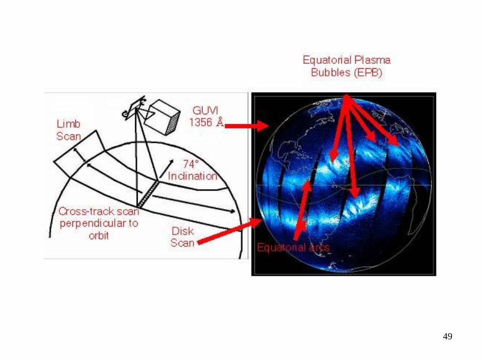
b. Equatorial region: plasma bubble
2. Ionospheric regions that can
disturb satellite communication

Blob
Bubble
Figure. Sample plots of bubbles and blobs observed by ROCSAT-1 [Le et al., 2003]. Plasma bubbles and blobs are the local plasma density reduction and enhancement, respectively, relative to the background.

In-situ ion density measurements
at 600 km from the ROCSAT satellite All-sky image in Brazil
Plasma bubble can affect
radio scintillation (GPS L1
frequency), S4, and TEC

a narrow band around equator that is affected by scintillations
Kennewell and McDonald [2010]
Note: the location of the band is determined from magnetic equator
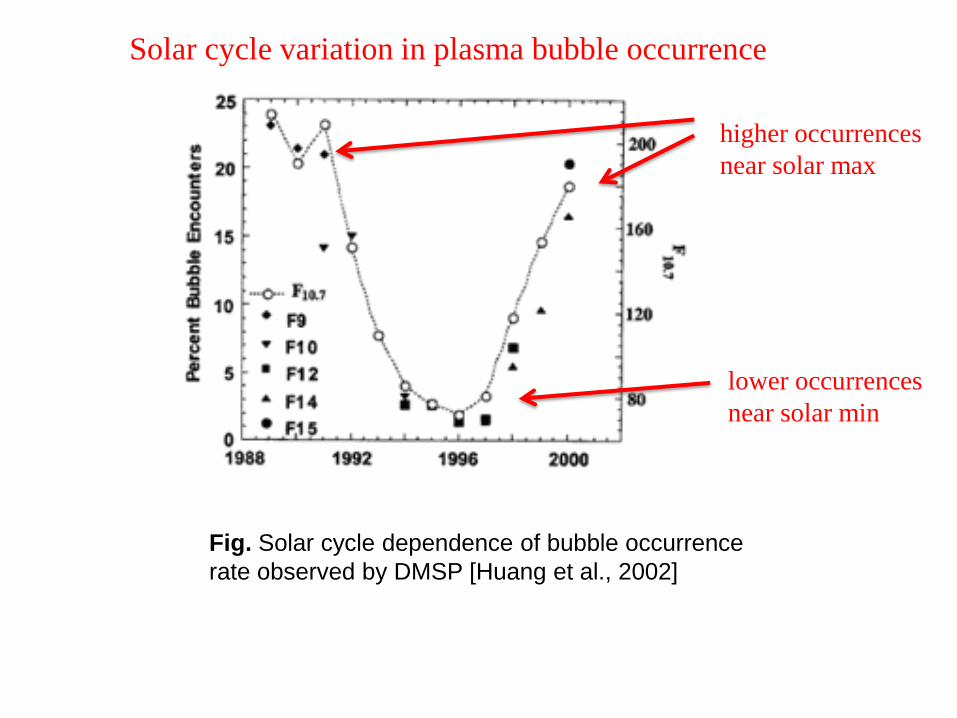
Fig. Solar cycle dependence of bubble occurrence
rate observed by DMSP [Huang et al., 2002]
higher occurrences
near solar max
lower occurrences
near solar min
Solar cycle variation in plasma bubble occurrence

Fig. Latitude distribution of
bubbles observed by
ROCSAT-1 [Su et al., 2006].
seasonal variation
in the occurrence of
plasma bubble
higher occurrences
near equinoxes

45
Stening [2003]
mlat = -12.6 deg
Parepare, Indonesia
higher S4
occurrences near
equinoxes 1998
1999

46
TIMED [LEO]
(Thermosphere, Ionosphere, Mesosphere Energetic Dynamics)
• Earth orbiter 625 km, measures UV to NIR
spectral radiance of Thermosphere,
Mesosphere, Ionosphere, 60-180 km
(intercept signatures, backgrounds)
• Launched December 2001, 2-year mission
• Autonomous onboard GPS navigation (no ground
tracking needed)
• Pulse cryocooler for optics (space qualification)
• UV spatial scanning spectrograph (shake down
algorithms for DMSP space sensing instrument)
• Doppler interferometer for wind and temperate
(moving target velocity)
SEE
TIDI
GUVI
SABER
(Solar Energy Inputs)
(Winds, Energy
Transport)
(Energy Outputs,
Pressure,
Temperature,
Composition)
(Auroral Energy
Inputs, Temperature,
Composition)
TIMED payloads are operated directly by scientists in a secure, authenticated manner, with autonomous deconfliction much like the vision for tactical commanders requesting space services

47
DMSP Satellite
DMSP satellite: • Nearly circular polar orbiting satellite at roughly 835 km.
• The SSJ4 instrument package detects precipitating ions and electrons
from 32 eV to 30 keV [Hardy et al., 1984] (the detector looks up).
• SSUSI instrument images in UV wavelengths
• One complete 19 point ion and electron spectrum is obtained for each
second, during which time the satellite moves ~7.5 km.
The Defense Meteorological Satellite
Program (DMSP) designs, builds,
launches, and maintains satellites
monitoring the meteorological,
oceanographic, and solar-terrestrial
physics environments.
Artist’s concept of the DMSP satellite

FUV spectrograph imaging technique used by
TIMED/GUVI and DMSP/SSUSI
49

Nighttime O I 135.6-nm radiance map produced by using
the TIMED/GUVI data.
The two distinguishing phenomena in the low-latitude F region are the
equatorial ionization anomaly (EIA) and equatorial plasma bubbles (EPB).
O+ + e O* O + 135.6-nm emission
EIA
bubble

Kil et al. [2009]

Fig. Test of the detection of a plasma depleted magnetic flux by
optical observations.
Kil et al. [2009]
the bubble image mainly reflects the condition at peak density altitude where the
contrast between depleted field line and its neighbors is the sharpest

Zonal shear exists in plasma drift
Fig. ROCSAT-1 observation of the zonal plasma drift at the altitude of
600 km (left) and the zonal distance traveled during 4 hours.
mean velocity at 2000-2400 LT
near 250°E in March 2002
in four hours, the bubble at
the equator would travel the
farthest longitudinally

The zonal shear flow of the ionosphere creates a
“plasma depletion shell”.
The intersection of the plasma depletion shell with horizontal
plane at F-peak altitude creates a backward C-shaped optical
bubble image.
Kil et al. [2009]

55 Kil et al. [2009]

Formation of a plasma depletion shell
TIMED/GUVI image
Plasma depletion shell
Kil et al. [2009]
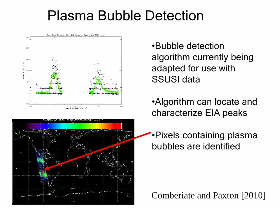
Plasma Bubble Detection
•Bubble detection
algorithm currently being
adapted for use with
SSUSI data
•Algorithm can locate and
characterize EIA peaks
•Pixels containing plasma
bubbles are identified
Comberiate and Paxton [2010]

SSUSI Observation Model
• Use tomography technique to obtain 3D images
• Assume invariance along field lines for that segment
• Distinct overlapping scans with respect to altitude vs. longitude profile allow for tomography

3-D Bubble Imaging Technique
•Tomographic inversion
performed for each
altitude vs. longitude slice
•12 slices (5° latitude
resolution) combined to
form 3D profile
•Main sources of error
include low SNR for
counting statistics, limited
latitudinal resolution, and
limited-angle viewing
geometry

SSUSI Bubble Imaging
Comberiate and Paxton [2010]

Bubble Formation
•Bottomside depletion visible in both images
•Plume growth (15 min between images)
•Depleted region drifts East at approx. 100 m/s
Comberiate and Paxton [2010]
TIMED GUVI and DMSP SSUSI have broken new grounds in plasma bubble studies

62
3. Space weather forecasting with
machine learning

63
The underlying physics of many space objects and phenomena is often
complex and not well understood, but progress can be achieved through the
use of advanced or even standard machine learning and artificial intelligence
principles
. .
.
I
N
P
U
T . . .
O
U
T
P
U
T
. .
.
I
N
P
U
T . . .
O
U
T
P
U
T
Physics
based
system
Machine
learning
or AI
based
system

64
Neural Network
• A NN architecture with 1 hidden layer [a class of multi-layer feedforward network (MLFN)]
A class of NN with 0 hidden layer is called perceptron
The intelligence lies in the connections
between the nodes

Two applications of neural
networks
65
a. Kp forecast models
b. HF backscatters from ionospheric irregularities
(clutters)

66
3.a Kp forecast models

Bhattacharyya and
Basu [2002]
geographic lat = 18 deg N
• Kp is a geomagnetic activity
index
• During storm, Kp is high
• TEC near noon is twice as
large as the previous day

68
Pandey and Dashora [2005]
Udaipur (mlat = 15.3 deg) near EIA
nightside dayside

69
Background and Motivations for developing Kp forecast models
• Moderate and high activities are notoriously difficult to predict [Joselyn, 1995].
• Real-time magnetometer data can be used to calculate nowcast Kps, which could improve the accuracy of the forecast Kps.
Why Kp?
• Kp is one of the most popular global indices.
• Kp has been playing significant roles in space weather, e.g., satellite drags, satellite communication, etc.
• Many magnetospheric and ionospheric models require Kp as an input parameter, e.g., T89 magnetic field model, Fok ring current-radiation belt model, MSFM, OVATION, etc.
• The long uninterrupted Kp record since 1932 makes it ideal for studying solar-wind magnetosphere interactions, e.g., the solar cycle effects, etc.

70
The APL Kp forecast models
. .
. Solar wind,
IMF,
[previous Kp]
Normaliz
ed Kp
NN
based
system
INPUT
OUTPUT

71
Summary and Conclusion
• In order to satisfy different needs and operational constraints, we developed 3 Kp forecast models: 1. APL model 1
• Input: ACE solar wind n, Vx, IMF |B|, Bz, and nowcast Kp • Output: ~1-hr ahead Kp forecast
2. APL model 2 • Input: same as model 1 • Output: ~4-hr ahead Kp forecast
3. APL model 3 • Input: ACE solar wind n, Vx, IMF |B|, and Bz • Output: ~1-hr ahead Kp forecast
• Note: a very accurate nowcast Kp algorithm [Takahashi et al., 2001] can
be used as an input to APL models 1 and 2.

72
Summary and Conclusion Boberg et al. [2000] Operational at Lund Obs.
Operational at NOAA/AF
APL model 1 APL model 3 (purely driven by solar wind)
APL model 2 (4 hr ahead forecast)
Univ. of Sheffield
Wing et al. [2005]

73
Predictive Model Performance
TSS xw yz
x y
zw
True Skill Statistics (TSS):
Gilbert Skill (GS):
GS ignores w (“correct rejection”). Ch = chance hits = (probability of Y events to occur) X
(number of Y events forecasted)
GS xCh
xCh
yz
Ch xy
x yzw
xz
For TSS and GS: Perfect forcecast = 1 Random forecast = 0
The figures show the skill scores for Costello
Neural Network (NN) model over 2 solar cycle
periods. They show that the model performance
has a solar cycle variation. The model performs
better near solarmax than solarmin for active times
(Kp > 3). The input parameters to the model are:
solar wind V, IMF |B|, IMF Bz, and the previous
Kp predictions of the model.
The skill scores are defined below (Detman and Joselyn, 1999).
The skill scores are defined below
(Detman and Joselyn, 1999).
Y N
Y x y
N w z Observed
Forecast

74
Summary and Conclusion
True Skill Statistic (TSS) [Detman and Joselyn, 1999] based on data spanning over 2 solar cycles.
Note: for comparisons with other published results, r is calculated over all Kp ranges and therefore, this figure understates the dramatic improvements the APL Kp models obtain for active times, Kp > 4.
Wing et al. [2005]

75
76
Solar cycle dependence of Kp
forecasts

77
Kp (magnetospheric) predictability as a function of solar cycle
• Papitashvilli et al. [2000] reports that there is solar cycle variation in the average Kp.
• It would be interesting to determine if the accuracy of Kp (a proxy for the magnetospheric state) forecast based partly or entirely on solar wind/IMF has solar cycle dependence.
• Calculate the skill scores (TSS and GS [Detman and Joselyn, 1999]) for Kp forecast models for 2 solar cycles, 1975-2000.

78
Kp predictability as a function of solar cycle
0 = random forecast
1 = perfect forecast
Costello NN Kp model predicts Kp more accurately near solar maximum than minimum.

79
Kp predictability as a function of solar cycle
The solar cycle dependence of APL model 3
While the scores are higher than those for Costello model, they still exhibit solar cycle variation, albeit with smaller amplitude.
Training with a larger data set cannot eliminate the solar cycle effect completely.
APL model 3 performs better during solar max than solar min.
Wing et al. [2005]

80
Kp predictability as a function of solar cycle
= SL ~ linear correlation [Kp(t), Kp(t - )] = SNL ~ nonlinear correlation
Solar minimum Solar maximum Cumulant based method analysis of the statistical informational dynamics of Kp time series.
The linear response is roughly equal, but the nonlinear response is stronger for solar min than solar max (peak ~ 40hr)
The magnetosphere is dominated more by internal dynamics during solar min than solar max, when it is more directly driven.

81
Kp predictability as a function of solar cycle
The nonlinear response anti-correlates with sunspot number in every solar cycle since Kp record is kept.

82
The Nonlinearity is not Intrinsic
to the Solar Wind
• Intrinsic solar wind
nonlinearity maximizes at
2 hours delay and is small
beyond 30 hours
• Kp peaks do not appear
related to intrinsic solar
wind nonlinearity
• Implication: the Kp
nonlinearity is the result of
internal dynamics

83
4. Summary • Space Weather is relevant at high and low latitude (e.g., Indonesia)
• can affect technologies and many daily activities
• can affect Palapa satellites: communication and spacecraft charging
• Space weather at the equatorial region has not been as well understood as polar region there is a lot of opportunities to make discoveries
• Ionospheric regions that disturb satellite communication:
• high latitude scintillation: aurora particle precipitation
• aurora dynamics
• can affect intercontinental air travel
• low latitude scintillation: plasma bubbles
• has solar cycle and seasonal variations
• TIMED GUVI and DMSP SSUSI
• 2D plasma bubble images
• 3D plasma density profiles
• sometimes appear as “backward C” in 2D images
84
4. Summary
• Machine learning is a powerful tool for space weather forecasting
• HF backscatters from ionospheric irregularities (clutters)
• Kp forecast models
• Extensive Kp model evaluations based on data spanning over 2 solar cycles suggest that
1. Kp is slightly more predictable during solar max than solar min.
2. Cumulant based information dynamics analysis of Kp shows that Kp (the magnetosphere state) is more strongly nonlinearly coupled with the past Kps during solar min than solar max [Johnson and Wing, 2004].
3. (1) and (2) suggest that the magnetosphere is more externally driven during solar max (declining phase of solar max) than solar min, when internal dynamics play a more significant role.

85